Embed Size (px)
Citation preview
Scale-Invariant Measures of Segregation�
David M. Frankel
Iowa State University
Oscar Volij
Ben Gurion University
August 7, 2008
Abstract
We characterize measures of school segregation for any number of ethnic groups
using a set of purely ordinal axioms that includes Scale Invariance: a school district�s
segregation ranking should be invariant to changes that do not a¤ect the distribution
of ethnic groups across schools. The symmetric Atkinson index is the unique such
measure that treats ethnic groups symmetrically and that ranks a district as weakly
more segregated if either (a) one of its schools is subdivided or (b) its students in a
subarea are moved around so as to weakly raise segregation in that subarea. If the
requirement of symmetry is dropped, one obtains the general Atkinson index. The role
of Scale Invariance is illustrated by studying segregation among U.S. public schools from
1987/8 to 2005/6, a period in which ethnic groups became distributed more similarly
across schools. While the Atkinson indices declined sharply, most other indices either
rose or declined only slightly.
�Email addresses: [email protected]; [email protected]. Volij thanks the Spanish Ministerio de
Educación y Ciencia (project SEJ2006-05455) for research support.

1 Introduction
Recent research supports the view that school segregation creates unequal opportunities:
separate schools are not equal. By and large, students in schools with a higher propor-
tion of minority students have lower educational attainment and subsequent wages (Boozer,
Krueger, and Wolkin [4, pp. 303-6]; Hanushek, Kain, and Rivkin [16]; Hoxby [17]). Consis-
tent with this, African Americans tend to have better educational outcomes in less segregated
school districts (Card and Rothstein [5]; Guryan [15]).1
While the e¤ects of school segregation are of great concern, there also rages, behind
the scenes, an intense controversy. It is over a more fundamental issue: how segregation
itself should be measured. One view of segregation, which we take in this paper, is that it
relates to how origins a¤ect destinations: how a student�s ethnic origin a¤ects which school
she ends up attending. To measure segregation, we must therefore look at the extent to
which ethnic groups are distributed di¤erently across schools. This notion is favored by the
sociologists James and Taeuber [22]. It corresponds to the �rst of Massey and Denton�s [28]
�ve dimensions of segregation, which they call �evenness�.2
In order to be true to the notion of evenness, we require that a measure be Scale Invariant:
that it rank a district based solely on how each ethnic group is distributed across the district�s
schools, and not on the proportions of di¤erent ethnic groups in the district. In explaining
this property, Taeuber and James write:
School segregation refers to racial variation in the distribution of students across
schools. ... This concept of segregation does not depend on the relative propor-
tions of blacks and whites in the [district], but only upon the relative distributions
of students among schools.... [Taeuber and James [38, p. 134]]
1Cutler and Glaeser [10] �nd similar e¤ects of residential segregation.
2Their second dimension is isolation of the minority group. The other three dimensions, which are more
relevant in a residential context, are concentration in a small area, centralization in the urban core, and
clustering in a contiguous enclave.
2
Scale Invariance is one of the �ve requirements that Jahn et al [21] say a satisfactory measure
of segregation should satisfy.3
One important context in which Scale Invariance is desirable is school desegregation.
How should a district�s progress in desegregation be judged? To be fair, we should not
penalize a district for factors that are out of its control, such as the size or growth rate of
its minority population. Accordingly, a Scale Invariant measure of segregation is needed.
This is not a trivial requirement: none of the commonly used segregation indices are Scale
Invariant in the general multigroup case.4
Formally, we de�ne a segregation ordering as a complete ordering on school districts: a
ranking of districts frommost segregated to least segregated. In addition to Scale Invariance,
we require this ordering to satisfy a few other simple axioms. Group Symmetry requires
that the segregation ordering be invariant to the renaming of the groups. The Weak School
Division Property states that in a school district that contains a single school, building a
new school to which some of the students are moved (a) cannot lower segregation in the
district, and (b) leaves segregation unchanged if the ethnic distributions of the two resulting
schools are identical. Finally, our Independence axiom states that if the students in a subset
of schools are reallocated within that subset, then segregation in the whole district rises if
and only if it rises within the subset.
These are all ordinal axioms: rules for how various operations should a¤ect a district�s
place in the segregation ordering. In contrast, the prior literature has generally imposed
cardinal axioms on the segregation index itself. Sometimes these properties have clear
ordinal implications, but often they do not. For example, what are the ordinal implications
of requiring that an index be additively separable? This problem is avoided by restricting
3They write: �a satisfactory measure of ecological segregation should ... not be distorted by the size of
the total population, the proportion of Negroes, or the area of a city....�(Jahn et al [21]).
4The Gini index and the usual formulation of the Dissimilarity index are Scale Invariant only in the
two-group case. The Entropy and Normalized Exposure indices are never Scale Invariant. See, e.g., the
survey in Reardon and Firebaugh [33].
3

to ordinal axioms.
Our main results are as follows. First, the ordering that is captured by the symmetric
Atkinson index is the unique nontrivial ordering that satis�es Group Symmetry, Scale In-
variance, the Weak School Division Property, and Independence. This index is de�ned as
one minus the sum, over all schools, of the geometric averages of the percentages of each
group who attend the school.5 For instance, suppose 40% of blacks, 70% of Hispanics,
and 10% of whites attend school A while the remainder attend school B. The index equals
1� (:4)1=3 (:7)1=3 (:1)1=3 � (:6)1=3 (:3)1=3 (:9)1=3.
We then drop the Group Symmetry axiom and characterize the set of orderings that
satisfy the remaining axioms, with the addition of a technical Continuity axiom. Each such
ordering is represented by an index of the following form: one minus the sum, over all the
schools, of some weighted geometric average of the percentages of each group who attend the
school. In the above example this would equal 1 � (:4)b (:7)h (:1)w � (:6)b (:3)h (:9)w where
b; h; and w are arbitrary nonnegative weights that sum to one. We will refer to this as the
general Atkinson index.
While the symmetric Atkinson index gives equal weight to all ethnic groups, the general
Atkinson index leaves these weights up to the researcher. For instance, one may desire an
index that is more sensitive to segregation between two large groups than two small groups.
Most multigroup segregation indices accomplish this by weighting a group according to the
group�s relative size in a given district. This violates Scale Invariance since a group�s weight
varies from one district to another. An alternative is to use an Atkinson index with weights
that vary across groups but not across districts. For instance, a group�s weight might equal
the proportion of students in the U.S. who belong to that group in some reference year.
Since the weight on each group is constant across districts, Scale Invariance is satis�ed.
5This is an increasing transformation of the original symmetric Atkinson index of James and Taeuber
[22] in the case of two ethnic groups. Hutchens [19] calls this version the Square Root Index. Since they
are related by an increasing transformation, the two versions represent the same ordering of school districts
(section 3).
4

We illustrate our results by studying changes in U.S. public school segregation from
1987/8 to 2005/6. We study the symmetric Atkinson index as well as two asymmetric
Atkinson indices that are based, respectively, on the ethnic distributions at the beginning and
end of the period. We �rst show, using Lorenz curves, that ethnic groups had more similar
distributions across public schools in 2005/6 than in 1987/8.6 By the evenness criterion,
school segregation should have fallen. Indeed, the Atkinson indices fell considerably over
the period. However, there was also another development: the proportion of whites in the
student population fell from 71% to 58%. This increase in ethnic diversity has no e¤ect on
the Atkinson indices as they are Scale Invariant. However, it tempered or even reversed
the declines of the multigroup versions of indices such as Dissimilarity, Gini, Entropy, and
Normalized Exposure, none of which are Scale Invariant in the multigroup case.7 As a
result, none of these indices fell as much as the Atkinson indices, and some of them rose
considerably.
The Atkinson segregation indices were introduced by James and Taeuber [22] and are
based on the Atkinson family of inequality indices (Atkinson [2]). Massey and Denton [28]
study properties of the Atkinson indices; Johnston, Poulsen, and Forrest [24] use them to
study residential segregation. While this literature has focused on the case of two ethnic
groups, we study the general multigroup case.
The �rst to study segregation axiomatically, Philipson [31], provides an axiomatic char-
acterization of a large family of segregation orderings that have an additively separable
representation. The representation consists of a weighted average of a function that depends
on a school�s demographic distribution only. Hutchens [18] characterizes the family of seg-
regation indices that satisfy a set of basic properties in the case of two ethnic groups. In a
subsequent paper, Hutchens [19] strengthens one axiom and obtains the symmetric Atkinson
6There is just one exception: the Lorenz curve for blacks vs. whites for the two years intersect. However,
they are very close to one another.
7There is a Scale Invariant version of the Dissimilarity index that does decline over the period (section
3.2). However, this version is not in common use.
5

index. While we assume properties of the underlying segregation ordering, Hutchens follows
the inequality literature (e.g., Shorrocks [36, 37]) by imposing restrictions directly on the
segregation index. Echenique and Fryer [13] characterize an index that uses social network
data to measure the strength of an individual�s isolation from members of other demographic
groups. They also rely on cardinal axioms.
None of our axioms relate to comparisons between districts that have di¤erent numbers
of ethnic groups. Thus, we can say nothing about how such districts should be ranked.
Frankel and Volij [14] allow a variable number of ethnic groups by assuming the Group
Division Property: if a given ethnic group is subdivided into two groups that have the same
distribution across schools, then the segregation of the district should not change. However,
they drop Scale Invariance as the two axioms together have implausible implications.8
The paper is organized as follows. Concepts and notation are de�ned in Section 2.
Section 3 gives examples of segregation indices. Section 4 presents the axioms. Theoretical
results appear in section 5 and empirical �ndings in section 6. We conclude in section 7.
Proofs are relegated to an appendix.
2 De�nitions
We assume a continuum population. This is a reasonable approximation when ethnic groups
are large. In our examples, each �person�should be interpreted as representing some large,
�xed number of students.
Formally, we de�ne a (school) district as follows:
De�nition 1 A district X consists of
� A nonempty and �nite set of schools N and ethnic groups G. (We will write N(X)
when necessary to avoid ambiguity.)
8Together, the axioms permit one to scale a group up and then split it into identically distributed groups
- thus making endless copies of the original group - without changing a district�s segregation ranking.
6

� For each ethnic group g 2 G and for each school n 2 N, a real number T ng � 0: the
number of members of ethnic group g that attend school n.
We will sometimes specify a district as a list of ethnic compositions of schools in the
district. For instance, h(10; 20) ; (30; 10)i denotes a district with two schools and two ethnic
groups - say, blacks and whites. The �rst school, (10; 20), contains ten blacks and twenty
whites; the second, (30; 10), contains thirty blacks and ten whites.
For any nonnegative scalar �, �X denotes the district in which the number of students
in each group and school has been multiplied by �. If Y is another district, X ] Y denotes
the result of combining districts X and Y . For example, if X = h(10; 20) ; (30; 10)i and
Y = h(40; 50)i, then 2X = h(20; 40) ; (60; 20)i, and X ] Y = h(10; 20) ; (30; 10) ; (40; 50)i.
The following notation will be useful:
Tg =Xn2N
T ng : the number of students in ethnic group g in the district
T n =Xg2G
T ng : the total number of students who attend school n
T =Xg2G
Tg: the total number of students in the district
Pg =TgT: the proportion of students in the district who are in ethnic group g
P n =T n
T: the proportion of students in the district who are in school n
png =T ngT n
(for T n > 0): the proportion of students in school n who are in ethnic group g
tng =T ngTg: the proportion of students in ethnic group g who attend school n
The ethnic distribution of a district X is the vector P = (Pg)g2G of proportions of the
students in the district who are in each ethnic group. The ethnic distribution of a nonempty
school n is the vector pn =�png�g2G of proportions of students in school n who are in each
ethnic group. A school is representative if it has the same ethnic distribution as the district
that contains it.
7

3 Examples of Segregation Indices
3.1 Atkinson Indices
The Atkinson segregation indices were introduced by James and Taeuber [22] for the case
of two ethnic groups. They are based on the Atkinson inequality indices (Atkinson [2]).9
Let w = (w1 : : : wK) be a vector of K nonnegative weights that sum to one. The general
Atkinson index with weights w, Aw, is de�ned by
Aw(X) = 1�X
n2N(X)
Yg2G
�tng�wg (1)
The symmetric Atkinson index is obtained when all the weights are equal:
A(X) = 1�X
n2N(X)
�Yg2G
tng
� 1K
(2)
3.2 Unweighted Dissimilarity
In the case of two groups, the Index of Dissimilarity (Jahn et al [21]) equals the proportion of
either group who would have to change schools in order to attain complete integration. This
index was used by Cutler, Glaeser, and Vigdor [11] to measure the evolution of segregation
in American cities. Its usual generalization to three or more groups gives more weight to
larger groups and is due to Morgan [30] and Sakoda [35] (see section 6). Another possible
generalization, which we call the Unweighted Dissimilarity index, is de�ned by
DU(X) =1
2(K � 1)X
n2N(X)
f(tn) where f(tn) =Xg2G
�����tng �Xg02G
1
Ktng0
����� (3)
This generalization gives the same weight to each ethnic group.
9In the case of two groups, the Atkinson index with weight 0 < � < 1 on group one equals
1 �hP
n2N(X) (tn1 )�(tn2 )
1��i 11��
(James and Taeuber [22, p. 9]). This index is di¢ cult to generalize to
more than two groups since the outer exponent, 11�� , is the reciprocal of the weight on a particular ethnic
group. Instead, we generalize 1 �P
n2N(X) (tn1 )�(tn2 )
1��. This is an increasing transformation of the
original index and thus represents the same ordering.
8

3.3 Mutual Information
The entropy of the discrete probability distribution q = (q1; : : : ; qK) is de�ned by10
h(q) =
KXk=1
qk log2
�1
qk
�:
The Mutual Information Index equals the entropy of a district�s ethnic distribution minus
the average entropy of the ethnic distributions of its schools:
M(X) = h(P )�X
n2N(X)
P nh(pn)
where P = (Pg)g2G is the district ethnic distribution and pn = (png )g2G is the ethnic distrib-
ution of school n. This index was �rst proposed by Theil [39] and is axiomatized in Frankel
and Volij [14].
4 Axioms
We now introduce our axioms. We restrict attention to districts that have a �xed set of
ethnic groups with positive membership. More precisely, let G be a set of K � 2 ethnic
groups and let C be the set of all districts whose nonempty ethnic groups are exactly the
groups in G. A segregation ordering < on C is a complete and transitive binary relation onC. The statement X < Y means �district X is at least as segregated as district Y .� The
relations � and � are derived from < in the usual way.11
A related concept is the segregation index : a function S : C ! < that assigns to each dis-
trict a number that is interpreted as the district�s segregation level. The index S represents
the segregation ordering < if, for any two districts X; Y 2 C,
X < Y if and only if S(X) � S(Y ) (4)
Every index S induces a segregation ordering < that is de�ned by (4).
10When qk = 0, the term qk log2(1=qk) is assigned the value zero.
11That is X � Y if both X < Y and Y < X; X � Y if X < Y but not Y < X.
9

We impose axioms not on the segregation index but on the underlying segregation or-
dering. These approaches are not equivalent. As in utility theory, a segregation ordering
may be represented by more than one index, and there are segregation orderings that are
not captured by any index.
A district�s segregation ranking or simply its segregation is its place in the segregation
ordering. We will sometimes say that if a transformation � : C ! C is applied to a district
X, then �the segregation of the district is unchanged�or �the district�s segregation ranking
is una¤ected.� By this we mean that �(X) � X. If this holds for all districts X, then we
will say that the segregation in a district is invariant to the transformation �.
Our �rst axiom, Scale Invariance, requires that an ordering be insensitive to changes in
the size of an ethnic group that leave that group�s distribution across schools unchanged.
More precisely:
Scale Invariance (SI) For any district X 2 C, group g 2 G, and constant � > 0, let X 0
be the result of multiplying the number of group-g students in each school n in district
X by �. Then X 0 � X.
The axiom of Independence states that if the students in a subarea of a district are
reallocated among schools within that subarea, then segregation in the district rises if and
only if segregation in the subarea rises:
Independence (IND) Let X; Y 2 C have equal populations and equal group distributions.
Then for any Z 2 C, X ] Z < Y ] Z if and only if X < Y .
Since X and Y have the same number of each ethnic group, Y ] Z is the result of real-
locating the students within the subarea X of the district X ] Z.12 The Dissimilarity
Index violates this principle. For instance, suppose a district is composed of two areas:
X = h(50; 100) ; (50; 0)i and Z = h(100; 0)i. Suppose that the students in the �rst area are
12IND does not require Y to have the same number of schools as X. Hence, the reallocation might be
accompanied by new school construction or conversion of some schools to other uses.
10

reallocated to yield Y = h(100; 40) ; (0; 60)i. The Dissimilarity Index within this area rises
from 0:5 to 0:6, but the index for the full district falls, counterintuitively, from 0:75 to 0:6.13
Independence rules out this behavior. In Section 5.2 we show that Independence is also a
precondition for an index to be additively decomposable in a sense discussed by Hutchens
[18].
The next axiom is the Weak School Division Property. This axiom states that a one-
school district cannot become less segregated if the school is split into two new schools. In
addition, if the new schools have identical ethnic distributions, then segregation is unchanged.
Intuitively, since a district that contains a single school is not segregated at all, splitting the
school cannot lead to lower segregation.14 And if the new schools have the same ethnic
distribution, then the new district is not segregated at all, like the original district.
Weak School Division Property (WSDP) LetX 2 C be a district consisting of a single
school. LetX 0 be the district that results from subdividing this school into two schools,
n1 and n2. Then, X 0 < X. Further, if n1 and n2 have the same group distributions(i.e., pn1g = pn2g for all g 2 G), then X 0 � X.
This axiom implies, for instance, that a district with 110 whites and ten blacks in a single
school does not become more segregated if the ten blacks and an equal number of whites
are relocated to a second school: the district h(110; 10)i is no more segregated than the
district h(100; 0) ; (10; 10)i. Of course, one can think of notions of �segregation�that would
contradict this. A student in the school (10; 10) might think that her new environment is
more �integrated�since it has equal numbers of blacks and whites. No model can capture all
possible notions of segregation. By Massey and Denton�s [28] evenness criterion, segregation
13The two versions of the Dissimilarity index coincide in this example since there are only two ethnic
groups. They equal the percentage of either group that must change schools in order for all schools to have
the same ethnic distribution.
14Our motivating example uses schools as the basic locational unit, so it ignores ability tracking and
other forms of within-school segregation. Our approach could easily be used to study these phenomena by
rede�ning basic locational unit to be the classroom or the ability group.
11
in the district has indeed increased: ethnic groups are (trivially) distributed evenly across
schools in the �rst district but not in the second.
WSDP is related to two properties that are discussed by James and Taeuber [22] and
subsequent authors. The �rst is organizational equivalence: if a school is divided into two
schools that have the same ethnic distribution, the district�s level of segregation does not
change. The second is the transfer principle. When there are two demographic groups, the
transfer principle states that if a black (white) student moves from one school to another
school in which the proportion of blacks (whites) is higher, then segregation in the district
rises. In the case of two ethnic groups, WSDP follows from organizational equivalence and
the transfer principle.15 But while WSDP applies directly with any number of groups, it is
unclear what form the transfer principle should take with more than two groups.16
Group Symmetry states that the level of segregation in a district does not depend on
the labeling of the district�s demographic groups; it depends only on the number of people
in each group who attend each school. For instance, if �blacks�are relabeled �whites�and
vice-versa, then segregation does not change.
Group Symmetry (GS) The segregation in a district is invariant to any relabeling or
reordering of the groups in the district.
We will consider axiomatizations both with and without this axiom.
Our next axiom, Continuity, will be needed only when Group Symmetry is dropped.
15A rough intuition runs as follows. The �rst part of WSDP is just organizational equivalence itself. As
for the second part, any division of a school into two new schools with di¤ering ethnic distributions can be
broken into two steps. First, create two schools with the desired sizes but the same ethnic distribution. By
organizational equivalence, segregation is unchanged. In the second step, swap black students with white
students until the desired ethnic distributions are attained. Since each swap moves students to schools in
which their groups are overrepresented, segregation must rise by the transfer principle.
16For instance, suppose a black student moves to a school that has higher proportions of both blacks and
Asians but fewer whites. Since there are more blacks, one might argue (using the transfer principle) that
segregation has gone up. On the other hand, blacks are now more integrated with Asians. One attempt to
overcome this di¢ culty appears in Reardon and Firebaugh [33].
12

Continuity (C) For any districts X;Y; Z 2 C, the sets
fc 2 [0; 1] : cX ] (1� c)Y < Zg and fc 2 [0; 1] : Z < cX ] (1� c)Y g
are closed.
Our �nal axiom states that there exist two districts, one strictly more segregated than
the other. It is needed to rule out the trivial segregation ordering.
Nontriviality (N) There exist districts X; Y 2 C such that X � Y .
5 Results
We �rst show that the general Atkinson index (equation (1)) satis�es all of the axioms
other than Group Symmetry. This axiom is satis�ed only by the symmetric Atkinson index
(equation (2)).
Proposition 1 Let w = (w1; : : : ; wK) be a list of K non-negative weights that add up to
one. The ordering represented by the general Atkinson index Aw satis�es SI, IND, WSDP,
N, and C. The ordering represented by the symmetric Atkinson index A also satis�es GS.
The next two theorems are the main results of our paper. Theorem 1 states that our set
of axioms, less Group Symmetry, fully characterizes the general Atkinson index.
Theorem 1 Let < be an ordering on C that satis�es SI, IND, WSDP, N, and C. There are�xed weights wg � 0 for g = 1; :::; K, adding up to one, such that < is represented by the
general Atkinson index Aw(X).
An easy implication of Theorem 1 is that if the requirement of Group Symmetry is added,
then the weights wg must all be equal. Hence, the symmetric Atkinson index represents the
unique ordering that satis�es this larger set of axioms. It turns out that this is still true if
Continuity is dropped. This is the following result.
Theorem 2 The ordering represented by the symmetric Atkinson index on C is the only
ordering that satis�es GS, SI, WSDP, IND, and N.
13
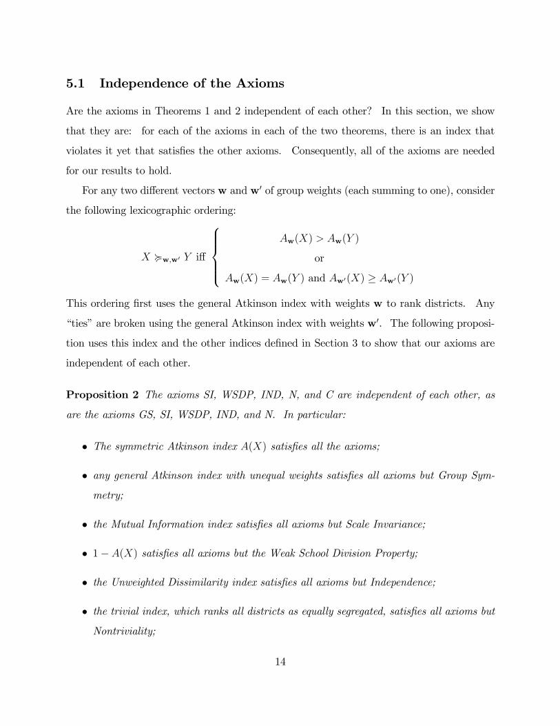
5.1 Independence of the Axioms
Are the axioms in Theorems 1 and 2 independent of each other? In this section, we show
that they are: for each of the axioms in each of the two theorems, there is an index that
violates it yet that satis�es the other axioms. Consequently, all of the axioms are needed
for our results to hold.
For any two di¤erent vectors w and w0 of group weights (each summing to one), consider
the following lexicographic ordering:
X <w;w0 Y i¤
8>>><>>>:Aw(X) > Aw(Y )
or
Aw(X) = Aw(Y ) and Aw0(X) � Aw0(Y )
This ordering �rst uses the general Atkinson index with weights w to rank districts. Any
�ties�are broken using the general Atkinson index with weights w0. The following proposi-
tion uses this index and the other indices de�ned in Section 3 to show that our axioms are
independent of each other.
Proposition 2 The axioms SI, WSDP, IND, N, and C are independent of each other, as
are the axioms GS, SI, WSDP, IND, and N. In particular:
� The symmetric Atkinson index A(X) satis�es all the axioms;
� any general Atkinson index with unequal weights satis�es all axioms but Group Sym-
metry;
� the Mutual Information index satis�es all axioms but Scale Invariance;
� 1� A(X) satis�es all axioms but the Weak School Division Property;
� the Unweighted Dissimilarity index satis�es all axioms but Independence;
� the trivial index, which ranks all districts as equally segregated, satis�es all axioms but
Nontriviality;
14

� the lexicographic index <w;w0, for weights w 6= w0, satis�es all axioms but Group
Symmetry and Continuity (so C is independent of SI, WSDP, IND, N).
This proposition is summarized in Table 1. A check mark indicates that an index satis�es
a given axiom; an � indicates that it does not.
GS SI WSDP IND N C
Symmetric Atkinson: A(X)p p p p p p
Aw(X) for w 6= (1=K; : : : 1=K) �p p p p p
Mutual Information M(X)p
�p p p p
1�A(X)p p
�p p p
Unweighted Dissimilarity: DU (X)p p p
�p p
Trivial indexp p p p
�p
Lexicographic <w;w0 for w 6= w0 �p p p p
�
Table 1: Independence of the axioms.
5.2 Additive Decomposability
It is often necessary to study segregation at several levels simultaneously. For instance, one
may be interested in how much of the segregation between classrooms in a district is due
to residential segregation and how much is due to ability tracking within schools. As a
�rst approximation, one might want to decompose total segregation into between-school and
within-school, between-classroom segregation. It turns out that only indices that satisfy
Independence can be decomposed in this way. This includes the Atkinson indices but not,
e.g., the Unweighted Dissimilarity index.
For any district Z, let the lower-case letter z denote the one-school district that results
from combining the students of Z into a single school. Following Hutchens [18], we say that
the segregation index S is additively decomposable if, for any (nonempty) districts X and Y ,
S(X ] Y ) = S(x ] y) + �(x; y)S(X) + �(x; y)S(Y ) (5)
15

where �(x; y) and �(x; y) are strictly positive numbers that depend only on the numbers of
students in each ethnic group in districts X and Y . That is, the segregation of the combined
district X ] Y can be written as the sum of segregation between the districts, S(x] y), and
the weighted sum of segregation within the districts X and Y , where the weights �(x; y)
and �(x; y) can depend on the sizes and ethnic distributions of X and Y but not on the
allocations of students across schools within X and Y .
Proposition 3 Suppose S is an additively decomposable segregation index. Then the or-
dering represented by S satis�es Independence.
The general Atkinson index with weights w = (w1; :::; wK) satis�es (5). More generally,
let Z = X1 ] � � � ]Xt, where each Xi is a district. Then it is straightforward to verify that
Aw(Z) = Aw(x1 ] � � � ] xt) +tXi=1
�iAw(Xi)
where xi is the district that results from combining the students in Xi into a single school
and �i =Qg2G
�Tg(xi)
Tg(z)
�wg.
Frankel and Volij [14] discuss a stronger type of additive separability, in which the weight
�i equals the proportion of students who are in district i. This stronger property is not
satis�ed by the Atkinson indices or, indeed, by any of the other common segregation indices
except Mutual Information (Frankel and Volij [14]).
6 Empirical School Segregation Patterns
In this section we study the change in school segregation in the U.S. between the 1987/8
and 2005/6 school years. The data source is the Common Core of Data (Sable, Gaviola,
and Garofano [34]). The set of reporting schools expanded considerably over the period,
making longitudinal comparisons hard to interpret. Accordingly, we restricted to the 62,519
schools that reported positive attendance in every school year from 1987/8 to 2005/6.17 We
17To aid in matching, for 1987/8 through 1998/99 we used the 13-year longitudinal version of this database
(McLaughlin [29]). For subsequent years, we used the annual �les. Schools that closed for one or more
16

use four, mutually exclusive ethnic groups: Asians, (non-Hispanic) whites, (non-Hispanic)
blacks, and Hispanics.18
We trace changes in three sets of indices. The �rst set is the Scale Invariant indices:
the Atkinson indices and the Unweighted Dissimilarity Index (section 3). Indices not in
this set fall, heuristically, into two groups. Each such index begins with a quantity that
captures some intuitive notion of segregation. Sometimes this quantity itself is used as the
segregation index: the index is unnormalized. This may be because the index already takes a
maximum value of one, or because normalization destroys certain desirable properties. This
set consists of the Card-Rothstein Index, the Clotfelter Index, and the Mutual Information
index. In other cases, the intuitive quantity is normalized by dividing by the maximum value
it can take, given the district�s ethnic distribution. This set consists of the Gini Index, the
Weighted Dissimiliarity Index, the Normalized Exposure Index, and the Entropy Index.19
Over the period we study, school segregation measures were a¤ected by two important
developments. First, the distributions of di¤erent ethnic groups across schools in the U.S.
became increasingly similar. Accordingly, the Scale Invariant indices show steep declines in
segregation over the full period. At the same time, ethnic diversity was growing signi�cantly.
Most strikingly, the proportion of Hispanic students rose from 10% in 1987/8 to 19.3% in
2005/6. This change dominated for the unnormalized Scale-Variant indices: they show
large increases over the period. As for the normalized Scale-Variant indices, increased
ethnic diversity led to o¤setting increases in both the intuitive quantities on which these
index are based, as well as the maximum possible values of these quantities. The end result
was little discernible change in the indices themselves.
years and then reopened are excluded from our sample. Since parents and teachers may prefer not to move
back after they have gotten used to new schools, the sense in which these are actually �the same schools�is
open to debate.
18The CCD actually has �ve ethnic groups; the smallest, American Indian/Alaskan Native, is not repre-
sented in some school districts. Hence, we include this group with the second smallest group, Asians.
19Frankel and Volij [14] study which of our axioms, among others, are satis�ed by these indices.
17

6.1 Unnormalized Scale-Variant Indices
The unnormalized Scale-Variant indices consist of the Mutual Information Index and two
other indices. Clotfelter [7] uses the percentage of black students who attend schools in
which at least some proportion � of students are black or Hispanic. We follow Clotfelter
[7] by using the two thresholds � = 0:5 and � = 0:9. Card and Rothstein [5] compute the
average fraction black or Hispanic in the schools attended by the typical black and white
student, and de�ne their segregation index as the di¤erence between these �gures. Letting
whites, blacks, and Hispanics be indexed by 1, 2, and 3, respectively, the Card-Rothstein
Index equals20
CR =Xn2N
�T n2T2� T
n1
T1
�T n2 + T
n3
T n
6.2 Normalized Scale-Variant Indices
We consider four normalized Scale-Variant indices. The Weighted Dissimilarity Index of
Morgan [30] and Sakoda [35] is de�ned as follows:
DW =1
ID0 where D0 =
1
2
Xg2G
Xn2N
P n��png � Pg�� (6)
and I is the Simpson Iteraction Index, I =P
g2G Pg(1�Pg) (Lieberson [26]). Intuitively, D0
equals the minimum proportion of the population that would have to change schools, keeping
school sizes �xed, in order for each school to be representative of the district. I is what
this proportion would be under complete segregation. Hence, the Weighted Dissimilarity
Index, DW , is a normalization of D0 that take a maximum value of 1.
The multigroup Gini Index of Reardon [32], is a generalization of the two-group Gini
index of Jahn, Schmidt, and Schrag [21]:
20In our application, Asians are included in the total school population, Tn.
18

G =1
IG0 where G0 =
1
2
Xg2G
Xm2N
Xn2N
PmP n��pmg � png ��
G0 is a measure of the extent to which the proportion in a given group varies across schools.
More precisely, it is the weighted sum, over all ethnic groups g and all school-pairs, of the
absolute di¤erence between the proportions in the two schools who are in group g. The
Gini index results from dividing this measure by its maximum value, I.
The Normalized Exposure Index was originally proposed by Bell [3] for the case of two
groups. Its multigroup version, formulated by James [23], is
P =Xg2G
Xn2N
P n(png � Pg)2
1� Pg
In the case of two groups (say blacks and whites, denoted 1 and 2, respectively), the index
equals P2�E�P2
where E� = 1T1
Pn2N T
n1 p
n2 is the proportion white in the school attended by
the average black student and P2 (the proportion white in the district) is the maximum
value of E� given the district ethnic distribution. Thus, the two-group index measures the
exposure of blacks to whites, normalized by the maximum possible such exposure. The
index is symmetric: it also measures the normalized exposure of whites to blacks.
Finally, the Entropy Index H (Theil [40]; Theil and Finizza [41]) is the result of dividing
the Mutual Information Index, M (section 3), by its maximum value, the entropy of the
district ethnic distribution: H =M=h(P ).
6.3 Findings
We study total segregation among U.S. schools, essentially treating the U.S. as a single
district and studying its evolution over time. In contrast, the literature has typically focused
on averages of city-level segregation indices. Despite its intuitive appeal, this common
approach is generally not well founded. In most cases, the resulting average does not equal
the within-city component of total segregation between U.S. schools: most segregation
19

indices are not decomposable into a within-city average plus a between-city term.21 In
addition, individual city-level indices often have an intuitive meaning that is lost when taking
their average across cities. This is particularly true when, as is often the case, normalized
indices are used.22
Multigroup segregation was a¤ected by two trends during the period we study. The
�rst is a decline in segregation between pairs of ethnic groups. Table 2 depicts the Lorenz
curves between each pair of students in 1987/8 and 2005/6. For each pair except blacks
and whites, the Lorenz curve rose over the period, indicating that the groups�distributions
across schools were becoming increasingly similar. Indeed, pairwise Gini indices fell for all
groups, as shown in panel 1 of Table 3.23 For blacks vs. whites, the two curves cross and
are close to one another: the change in the Gini index is only -0.005. The 2005/6 curve is
higher in schools with moderately high black percentages and lower in the schools with the
highest proportions black. This indicates a relative movement of whites into the former set
of schools and out of the latter set.
Over the period, there was another important development: minority groups grew in
relative terms. In 1987/8, the proportions of Asians, blacks, and Hispanics in U.S. schools
were 4.0%, 15.3%, and 10.0%, respectively. By 2005/6, these percentages had grown to
5.7%, 16.8%, and 19.3%, respectively, while the percentage of whites had fallen from 70.8%
21Indices that violate Independence are not decomposable into within and between terms (section 5.2).
These include the Gini Index, the Card-Rothstein Index, the Normalized Exposure Index with three or more
ethnic groups, and the Weighted Dissimilarity Index (Frankel and Volij [14]). Unweighted Dissimilarity is
also in this category (section 5.1).
22To see the e¤ects of normalization, consider the population-weighted average of the unnormalized dissim-
ilarity index D0 de�ned in equation (6). This average does have an intuition: it is the minimum proportion
of students in the country who would have to change schools within their given cities, keeping school sizes
�xed, in order for each school to be representative of its city. In contrast, it is hard to �nd any intuition for
the average across cities of the normalized index, DW .
23The pairwise Gini index equals the area between the 45 degree line and the Lorenz curve, as a fraction
of the total area that lies below the 45 degree line.
20

to 58.2%. These �gures appear in panel 2 of in Table 3.
Panel 3 of Table 3 shows changes in the Scale Invariant segregation indices. These indices
are insensitive to changes in the ethnic distribution, so they would be expected to decline in
response to the increasing similarity in the ethnic groups�distributions across schools (Table
2). They consist of the Unweighted Index of Dissimilarity (UIOD), the symmetric Atkinson
index (ATKSYM), and two di¤erent versions of the general Atkinson index: one in which
a group�s weight equals its share in the universe of districts in 1987/8 (ATK87) and one in
which its weight equals its share in this universe in 2005/6 (ATK05). As anticipated, all of
these indices declined over the period.
Unnormalized Scale-Variant indices are shown in panel 4 of Table 3. These indices
consist of the Mutual Information Index (M), the Clotfelter Index with thresholds of 50%
(Cl50) and 90% (Cl90), and the Card-Rothstein Index (CR). Falling bilateral segregation
should cause these indices to fall; on the other hand, increased ethnic diversity tends to have
the opposite e¤ect. Over the 18-year period, the second e¤ect dominates: all indices show
increases.
For instance, the increase in the Mutual Information index shows that a randomly selected
student�s school now conveys more information about her race (Frankel and Volij [14]). This
is driven by the fact that there is now more information to convey: since ethnic diversity has
increased, the initial uncertainty about a random student�s race is now greater. Similarly,
the increase in the Clotfelter indices shows that a higher percentage of black students now
attend schools in which at least a given threshold (50% and 90%) of students are black or
Hispanic. This is driven by the increase in the proportions of blacks and Hispanics in the
U.S. student population. Finally, the increase in the Card-Rothstein index shows that the
absolute di¤erence in the proportion of minorities in the school attended by the typical black
vs. white student has grown. This is driven by two factors: growth in the proportion of
minority students in the U.S., combined with the lack of progress in black-white integration
(Table 2).
Normalized Scale-Variant indices appear in panel 5 of Table 3. This set consists of the
21

Gini Index (GINI), the Weighted Index of Dissimilarity (WIOD), the Normalized Exposure
Index (NEXP), and the Entropy Index (ENT). Each index equals the ratio of some intuitive
quantity to its maximum possible value. These indices show little change over the period.
In each case, greater ethnic diversity caused o¤setting increases in the intuitive quantity as
well as in its maximum possible value, with little change in the ratio.
In particular, the Weighted Index of Dissimilarity equals the proportion of students who
would have to change schools to attain perfect integration (D0), divided by the maximum
possible value of this proportion (I, the Simpson interaction index). While D0 rose from
0.301 to 0.370, I also rose, from 0.464 to 0.593 (Table 3, last panel). Their ratio, WIOD, fell
only slightly, from 0.648 to 0.624. Similarly, the Gini Index fell slightly, from 0.818 to 0.793.
It equals the ratio of the weighted-average absolute di¤erence in ethnic group proportions
(G0), which rose from 0.38 to 0.47, divided by the maximum possible value of this weighted
average (also the Simpson interaction index, I), which also rose, from 0.464 to 0.593 (panel 6
of Table 3). The Entropy Index fell from 0.456 to 0.429; it equals the expected information
a randomly selected student�s school reveals about her race (the Mutual Information Index),
which rose from 0.586 to 0.679, divided by total information present in a random student�s
race (the entropy of the overall ethnic distribution), which rose from 1.285 to 1.582 (panel 6
of Table 3).24
7 Conclusion
In this paper we have provided an axiomatic foundation for the Atkinson family of segrega-
tion orderings in the multigroup setting, using a parsimonious set of purely ordinal axioms.
We have shown that the ordering represented by the symmetric Atkinson index is the only
(nontrivial) segregation ordering that satis�es Group Symmetry, Scale Invariance, the Weak
School Division Property, and Independence. We also showed that a (nontrivial) segre-
24The Normalized Exposure Index lacks such a simple interpretation since di¤erent normalization factors
are applied to di¤erent terms in the sum.
22

gation ordering is represented by an index in the general Atkinson family if and only if it
satis�es Scale Invariance, the Weak School Division Property, Independence, and a technical
continuity property.
While the Atkinson indices are Scale-Invariant, most other multigroup segregation in-
dices are not. We illustrate the role of Scale Invariance by studying changes in the total
segregation of U.S. public school students from 1987/8 to 2005/6. For each pair of ethnic
groups except blacks and whites, the Lorenz curve rose: the groups�s distributions across
schools became more similar. This constitutes a decline in bilateral segregation accord-
ing to Massey and Denton�s [28] criterion of evenness. Consistent with this, the Atkinson
indices fell considerably over the period. On the other hand, there were large increases
in the proportions of all minority groups, especially Hispanics, who overtook blacks as the
second-largest ethnic group. This growth in ethnic diversity caused indices that are not
Scale-Invariant to rise or remain essentially unchanged.
A Proofs
For any district X and any nonnegative constant c, let cX denote the district that results
from multiplying the number of members of each group in each school of X by c. For
any district X and any vector of nonnegative scalars �!� = (�g)g2G, let�!� � X denote the
district in which the number of members of group g in school n is �gT ng . For example, if
X = h(1; 2) ; (3; 4)i, and �!� = (2; 3), then �!� � X = h(2; 6) ; (6; 12)i. We sometimes apply
the same operation to individual schools; e.g., �!� � (1; 2) = (2; 6).
We �rst de�ne a slight strengthening of WSDP:
School Division Property (SDP) Let X 2 C be any district and let n be a school in X.
Let X 0 be the district that results from X if school n is subdivided into two schools,
n1 and n2. Then, X 0 < X. Further, if n1 and n2 have the same group distributions(i.e., pn1g = pn2g for all g 2 G), then X 0 � X.
SDP follows from WSDP and IND:
23

Lemma 1 Suppose the segregation ordering < satis�es Independence and the Weak School
Division Property. Then < also satis�es the School Division Property.
Proof. Let Y denote the district X less the school n:
X = Y ] hni
X 0 = Y ] hn1; n2i :
By WSDP, hn1; n2i < hni. By IND, Y ] hn1; n2i < Y ] hni. If n1 and n2 have the same
population distribution then the symbol < can be replaced by �. Q.E.D.
We now state and prove some additional lemmas.
Lemma 2 Let < be a segregation ordering on C that satis�es SDP and SI.
1. All districts in which every school is representative have the same degree of segregation
under <.
2. Any district in which every school is representative is weakly less segregated under <than any district in which some school is unrepresentative.
Proof.
1. Consider any district Y in which every school is representative. Number the schools
1; :::; N . For each i = 1; :::; N , let Yi be the district that results from Y when the �rst
i schools of Y are combined into a single school. By SDP, for each i = 1; :::; N � 1,
Yi � Yi+1. Hence, by transitivity, Y = Y1 � YN . YN contains a single school. But by
SI, any district with a single school is as segregated as any other district with a single
school.
2. Let Y be a district in which every school is representative and consider any district X
in which at least one school is unrepresentative. The above reasoning yields X < XN .
XN contains a single school, so it is representative. Therefore, by 1, X < Y .
24

Q.E.D.
Lemma 3 Let < be a segregation ordering on C that satis�es SDP and SI. All completely
segregated districts have the same degree of segregation under <, and are weakly more segre-gated than any district in which any school is mixed.
Proof. Consider a completely segregated district X. Let X 0 be the district that results
from X when, for each group g 2 G, all schools that contain only members of group g are
combined into a single school. (X 0 thus consists of K schools, each of which contains all
the members of a single group.) By iteratively applying SDP, X � X 0. By SI, X 0 is as
segregated as any other district that consists of K schools, each of which contains all the
members of a single group. This implies that all completely segregated districts have the
same degree of segregation.
Now any district that has at least one mixed school can be converted into a completely
segregated district by dividing each school n into K distinct schools, each of which includes
all and only the members of a single group. By SDP, this procedure results in a weakly
more segregated district. Q.E.D.
Let X be a district with K groups of unit size who all attend in the same school: X =�1; 1; : : : ; 1| {z }K groups
��. Let X be a district with K groups of unit size who all attend separate
schools:
X =
��1; 0; : : : ; 0| {z }K groups
�;�0; 1; 0; : : : ; 0| {z }
K groups
�; :::;
�0; :::; 0; 1| {z }K groups
�| {z }
K schools
�:
We say that a school is a ghetto if all its students belong to the same group. We �rst
state and prove some auxiliary results about districts with a single non-ghetto school. For
any scalar �, let X(�) denote the district �XU(1 � �)X. City X(�) contains one school
with � students of each group, and K ghettos, each with 1� � students. Similarly, for any
vector t = (t1; :::; tK) 2 [0; 1]K , let X(t) denote the district
t �XU(1� t) �X = ht; (1� t1; 0; :::; 0); (0; :::; 0; 1� tK)i
25

City X(t) consists of the non-ghetto school t, and for each group g, one ghetto with 1� tgstudents of group g.
Lemma 4 Let < be a segregation ordering on C that satis�es SDP, IND, N, and SI. Then
1. X � X;
2. for any �; � 2 [0; 1], � > �, X(�) � X(�):
Proof.
1. By N, there exist districts X and Y such that X � Y . By lemmas 2 and 3, X < X �
Y < X, so X � X.
2. By part 1 and SI, (� � �)X � (� � �)X. Since the numbers of members of each
group are equal in district X and in X, they are also equal in district (� � �)X and
in (�� �)X. So by IND,
�X ] (�� �)X ] (1� �)X � �X ] (�� �)X ] (1� �)X:
The result follows from the fact that, by SDP,
�X ] (�� �)X ] (1� �)X � �X ] (1� �)X
and
�X ] (�� �)X ] (1� �)X � �XU(1� �)X:
Q.E.D.
Lemma 5 Let t;v 2 [0; 1]K, such that t � v. Then, X(t) < X(v). If t = (t1; :::; tK) 2
(0; 1)K then X � X(t) � X.
Proof. Let t;v 2 [0; 1]K , such that t � v. Applying SDP twice, we obtain
X(t) = t �XU(1� t) �X
� t �XU(v � t) �X
U(1� v) �X
< v �XU(1� v) �X = X(v).
26

Assume now that t = (t1; :::; tK) 2 (0; 1)K , and let t = maxft1; :::; tKg, t = minft1; :::; tKg.
Then,
X � X(t) by Lemma 4
< X(t) since (t; : : : ; t) � t
< X(t) since t �(t; : : : ; t)
� X by Lemma 4.
Q.E.D.
Lemma 6 For any two vectors t;v 2 [0; 1]K and for any 2 (0; 1],
1. v�X(t)U(1� v) �X � X(v � t)
2. X(t)U(1� )X � X( t)
3. If for some � 2 [0; 1], X(t) � X(�), then X(v � t) � X(�v)
4. If for some � 2 [0; 1], X(t) � X(�), then X( t) � X( �)
Proof.
1. By de�nition of X(t) and by SDP,
v�X(t)U(1� v) �X = v�
�t�X
U(1� t) �X
�U(1� v) �X
� (v � t) �XU(1� v � t) �X
= X(v � t):
2. The proof is analogous to the previous one.
3. Now, if for some � 2 [0; 1], X(t) � X(�), then, by SI and IND
v�X(t)U(1� v) �X � v�X(�)
U(1� v) �X
which, by the previous steps, implies X(v � t) � X(�v).
4. The proof is analogous to the previous one.
Q.E.D.
27
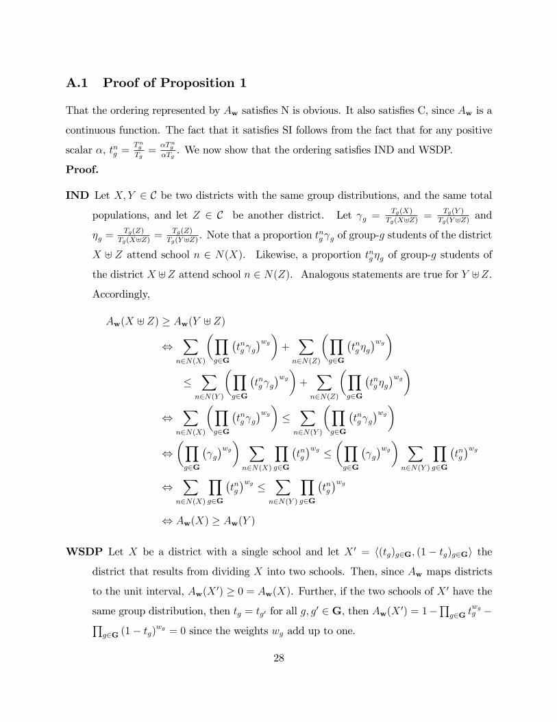
A.1 Proof of Proposition 1
That the ordering represented by Aw satis�es N is obvious. It also satis�es C, since Aw is a
continuous function. The fact that it satis�es SI follows from the fact that for any positive
scalar �, tng =TngTg=
�Tng�Tg. We now show that the ordering satis�es IND and WSDP.
Proof.
IND Let X; Y 2 C be two districts with the same group distributions, and the same total
populations, and let Z 2 C be another district. Let g =Tg(X)
Tg(X]Z) =Tg(Y )
Tg(Y ]Z) and
�g =Tg(Z)
Tg(X]Z) =Tg(Z)
Tg(Y ]Z) . Note that a proportion tng g of group-g students of the district
X ] Z attend school n 2 N(X). Likewise, a proportion tng�g of group-g students of
the district X ]Z attend school n 2 N(Z). Analogous statements are true for Y ]Z.
Accordingly,
Aw(X ] Z) � Aw(Y ] Z)
,X
n2N(X)
�Yg2G
�tng g
�wg�+X
n2N(Z)
�Yg2G
�tng�g
�wg�
�X
n2N(Y )
�Yg2G
�tng g
�wg�+X
n2N(Z)
�Yg2G
�tng�g
�wg�
,X
n2N(X)
�Yg2G
�tng g
�wg� � Xn2N(Y )
�Yg2G
�tng g
�wg�
,�Yg2G
� g�wg� X
n2N(X)
Yg2G
�tng�wg � �Y
g2G
� g�wg� X
n2N(Y )
Yg2G
�tng�wg
,X
n2N(X)
Yg2G
�tng�wg � X
n2N(Y )
Yg2G
�tng�wg
, Aw(X) � Aw(Y )
WSDP Let X be a district with a single school and let X 0 = h(tg)g2G; (1� tg)g2Gi the
district that results from dividing X into two schools. Then, since Aw maps districts
to the unit interval, Aw(X 0) � 0 = Aw(X). Further, if the two schools of X 0 have the
same group distribution, then tg = tg0 for all g; g0 2 G, then Aw(X 0) = 1�Qg2G t
wgg �Q
g2G (1� tg)wg = 0 since the weights wg add up to one.
28

GS Since the geometric average is a symmetric function, A satis�es GS.
Q.E.D.
A.2 Proof of Theorem 1
Let < be a segregation ordering on C that satis�es C, SDP, IND, N, and SI. We �rst buildan index that represents <. Later we show that the index has the requisite form.
Lemma 7 For any district X, there is a unique �X 2 [0; 1] such that X � X(�X).
Proof. By C,�� 2 [0; 1] : �X ] (1� �)X < X
and
�� 2 [0; 1] : X < �X ] (1� �)X
are closed sets. Any �X satis�es X � X(�X) if and only if it is in the intersection of these
two sets. The sets are each nonempty by Lemmas 2 and 3. Their union is the whole unit
interval since < is complete. Since the interval [0; 1] is connected, the intersection of the
two sets must be nonempty. By Lemma 4, their intersection cannot contain more than one
element. Thus, their intersection contains a single element �X . Q.E.D.
Let X and Y be two districts, and let �X , and �Y be the respective scalars identi�ed in
Lemma 7. Then, by Lemma 4, X < Y if and only if 1� �X > 1� �Y , which implies that
the index S : C ! [0; 1] de�ned by S(Z) = 1� �Z represents <.
We will now show that the index S has the requisite form.
Proposition 4 For each group g there is a �xed constant wg � 0 such that for any � 2 (0; 1],
X((1; : : : 1; �; 1; : : : 1)) � X(�wg)
where (1; : : : 1; �; 1; : : : 1) is a vector with � in the gth place and ones elsewhere.
Proof. For any scalar � and any group g, let �g denote the vector (1; : : : 1; �; 1; : : : 1) with
� in the gth place and ones elsewhere. Let hg : (0; 1]! <+ be the function de�ned by
X(�g) � X(hg(�)):
29

That is, for each � 2 (0; 1], hg(�) is the unique scalar � identi�ed in Lemma 7 such that
X(�g) � X(�). Let �; �0 2 (0; 1]. By Lemma 6 (parts 3 and 4), X(�g��0g) � X(hg(�0)�g) �
X(hg(�)hg(�0)). Therefore, hg satis�es the functional equation
hg(��0) = hg(�)hg(�
0) for all �; �0 2 (0; 1]: (7)
Further, by Lemma 5, if � < �0, then X(hg(�)) � X(�g) < X(�0g) � X(hg(�0)), which, byLemma 4 implies that hg(�) � hg(�
0). Therefore, hg is nondecreasing (and as a result it
is continuous at at least one point). The substitution � = e�u, �0 = e�v, hg(e�u) = f(u),
transforms (7) into
f(u+ v) = f(u)f(v) for all u; v � 0:
Therefore, by Theorem 1 in Aczél [1, pp. 38-39], either (a) f is identically 0, or (b) f(0) = 1
and, for all u > 0, f(u) = 0, or (c) there is wg such that f(u) = ewgu. This means that
either hg is identically 0, or hg(1) = 1, and hg(�) = 0 for � 2 (0; 1), or there is wg such that
hg(�) = �wg .
The function hg cannot be identically 0 because then, X = X(1; : : : ; 1) � X(hg(1)) �
X(0) = X, which contradicts nontriviality. Further, the function hg cannot be such that
hg(�) = 0 for � 2 (0; 1), because by Lemma 5 hg(�) � �. Therefore, using the fact that hgis nondecreasing there is wg � 0 such that hg(�) = �wg . Q.E.D.
Proposition 5 There are �xed, non-negative weights wg � 0 for g = 1; :::; K such that
for any t 2 [0; 1]K the unique � 2 [0; 1] that satis�es X(t) � X(�) is given byKQg=1
(tg)wg .
Further, the weights add up to one.
Proof. Case 1: t 2 (0; 1]K .
Let t = (t1; : : : ; tK) 2 (0; 1]K . By Proposition 4,
X((1; 1; : : : 1; tg; 1; : : : 1)) � X(twgg ) for all g = 1; : : : K:
Note that t =(t1; 1; :::; 1)�(1; t2; 1; : : : 1)�(1; : : : 1; tk). Then, repeated applications of Lemma 6
then yields
X(t) = X�QK
g=1 twgg
�:
30

In order to complete the proof of case 1, we need to show that the weights wg add up to
one. Consider the district X = X(�) where � 2 (0; 1). By the previous conclusion X �
X�QK
g=1 �wg�. By Lemma 4
�QKg=1 �
wg�= � which implies that the weights wg add up to
one.
Case 2: t 2 [0; 1]Kn(0; 1]K .
By Lemma 7 there is an � 2 [0; 1] such that X(t) � X(�). We need to show that � = 0.
Let t(") = (t1("); :::; tK(")) be the school that results from t after replacing the 0 components
by " > 0. Since t 2 (0; 1]K , by Case 1, X(t(")) � X(�(")) where �(") =QKg=1 tg(")
wg . By
Lemma 5, X(t) < X(t(")) which implies, X(�) < X(�(�)). By Lemma 4, �(�)) > � � 0.Since �(")! 0 as "! 0, we obtain that � = 0. Q.E.D.
We now show that the statement of the theorem holds for districts with two non-ghetto
schools.
Proposition 6 Let t1; t2 2 [0; 1]K and let X = ht1; t2; (1 � t11 � t21; 0; :::; 0); :::; (0; :::; 0; 1 �
t1K � t2K)i be a district. There is a unique �X 2 [0; 1] that satis�es X � X(�X). It is given
by �X =KQg=1
�t1g�wg
+KQg=1
�t2g�wg , where the weights wg are those found in Proposition 5.
Proof. Uniqueness of �X follow from Lemma 4, so it is enough to show that �X =KQg=1
�t1g�wg
+KQg=1
�t2g�wg satis�es X � X(�X). Assume �rst that tig � 1=2 for i = 1; 2 and
g = 1; :::; K. First suppose that tig = 0 for some i and g. Assume WLOG that t21 = 0.
Then by Proposition 5 and SI,
ht2; (1� t11 � t21; 0; :::; 0); :::; (0; :::; 0; 1� t1K � t2K)i � h(1� t11; 0; :::; 0); :::; (0; :::; 0; 1� t1K)i
so by IND, X � X(t1). The result then follows from Proposition 5.
Now suppose that t1; t2 2 (0; 1]K . Assume WLOG thatKQg=1
�t1g�wg � KQ
g=1
�t2g�wg . De�ne
etig = tig=(1 � t2g) for g = 1; :::; K and i = 1; 2. Note thatKQg=1
�et1g�wg � KQg=1
�et2g�wg . De�ne
� =KQg=1
�t1gt2g
�wg=
KQg=1
� et1get2g�wg
� 1. We can write
X = ht1; (1� t11 � t21; 0; :::; 0); (0; 1� t12 � t22; 0; :::; 0); :::; (0; :::; 0; 1� t1K � t2K)i ]t2�:
31

By SI
X � Y ]D�et21; :::;ft2K�E (8)
where25
Y =D�et11; :::;ft1K� ;�1� et11; 0; :::; 0� ; :::;�0; :::; 0; 1�ft1K�E
= et1 �XK ] (1� et1) �XK:
By Proposition 5,
Y � �YX ] (1� �Y )X: (9)
where �Y =KQg=1
�et1g�wg . De�neY 0 = � et2 �X ] (1� � et2) �X: (10)
We must verify that all entries in Y 0 are nonnegative. This holds if � et2g � 1 for all g. Sincet2g � 1=2 for all g, it follows that et2g � 1; since � � 1 as well, it follows that � et2g � 1.Since
KQg=1
�� et2g�wg = KQ
g=1
�et1g�wg = �Y , by Proposition 5,Y 0 � �YX ] (1� �Y )X: (11)
It follows from (9) and (11) that Y � Y 0. As a result,
X � Y ]�et21; :::;ft2K�� by (8)
� Y 0 ]�et21; :::;ft2K�� by IND
� � et2 �X ] (1� � et2) �X ] �et21; :::;ft2K�� by (10)
� (� + 1) et2 �X ] (1� � et2) �X by SDP
� (� + 1) t2 �X ] (1� (� + 1) t2) �X by SI and de�nition of et2:Therefore, using Proposition 5, X � �XX ] (1� �X)X, where
�X = (� + 1)
KYg=1
�t2g�wg
=KYg=1
�t1g�wg
+KYg=1
�t2g�wg
:
25We must check that Y has no negative entries. Since X cannot have negative entries, it must be that
t1g + t2g � 1 for all g. Since in addition t2g < 1 for all g, it follows that
t1g1�t2g
� 1 for all g. Hence, all entries
in Y are nonnegative.
32

Consider now the case of general t1; t2 2 [0; 1]2. De�ne bti = 12ti for i = 1; 2. Let
bX = hbt1;bt2; (1� bt11 � bt21; 0; :::; 0); (0; 1� bt12 � bt22; 0; :::; 0); :::; (0; :::; 0; 1� bt1K � bt2K)i:Each entry in each vector is at most one half. By the preceding argument, there is a uniqueb�X 2 [0; 1] such that bX � b�XX ] (1� b�X)X: (12)
and this unique b�X isKQg=1
�bt1g�wg + KQg=1
�bt2g�wg . Further note that by SDP, bX � 12X ] 1
2X.
Therefore
1
2X ] 1
2X � b�XX ] (1� b�X)X� 1
2(2b�X)X ] (1� 1
2(2b�X))X
� 1
2(2b�X)X ] 1
2(1� (2b�X))X ] 1
2X
where the last line follows from SDP. Finally, by IND and SI
X � (2b�X)X ] (1� (2b�X))Xwhich means that the unique �X that we are looking for is �X = 2b�X = KQ
g=1
�t1g�wg+
KQg=1
�t2g�wg .
Q.E.D.
Proposition 7 For every district X 2 C there is a unique �X 2 [0; 1] such that X �
�XX ] (1��X)X. Further, this unique �X isP
n2N(X)
KQg=1
�tng�wg , where the weights wg are
those found in Proposition 5.
Proof. By SI it is enough to prove the statement for districts where all groups have a
population measure of one. Also, by SDP we can restrict attention to districts where for
each group there is at most one ghetto. The proof is by induction on the number of non-
ghetto schools. Propositions 5 and 6 already show the that the statement is true for districts
with at most two non-ghetto schools. Assume that the statement of the theorem holds for
all districts with m� 1 non-ghetto schools, let
X = ht1; � � � ; tm; (1�mXn=1
tn1 ; 0; :::; 0); (0; 1�mXn=1
tn2 ; 0; :::; 0); :::; (0; :::; 0; 1�mXn=1
tnK)i
33

be a district with m non-ghetto schools. Then one can write
X = Y ] htmi
where Y denotes X with school tm removed. Y has m� 1 non-ghetto schools. By SI
Y ] htmi ���
1
1� tm1; ::;
1
1� tmK
�� Y�]��
tm11� tm1
; :::;tmK
1� tmK
��:
By the induction hypothesis,�
11�tm1
; :::; 11�tmK
��Y � �YX ] (1� �Y )X where
�Y =
m�1Xn=1
KYg=1
�tng
1� tmg
�wg:
Using (in order) IND, SI, and Proposition 6,��1
1� tm1; :::;
1
1� tmK
�� Y�]��
tm11� tm1
; :::;tmK
1� tmK
��� �YX ] (1� �Y )X ]
��tm1
1� tm1; :::;
tmK1� tmK
��� (1� tm1 ; :::; 1� tmK) �
��YX ] (1� �Y )X
�] htmi
� �XX ] (1� �X)X
where
�X =KYg=1
�1� tmg
�wg�Y +
KYg=1
�tmg�wg
=KYg=1
�1� tmg
�wg m�1Xn=1
KYg=1
�tng
1� tmg
�wg+
KYg=1
�tmg�wg
=
mXn=1
KYg=1
�tng�wg
:
Q.E.D.
This completes the proof of Theorem 1.
A.3 Proof of Theorem 2
Proposition 1 implies that the symmetric Atkinson index A satis�es all the axioms of the
theorem. We now show that it is the only index to do so. We now show that any ordering
34
that satis�es GS, SI, SDP, IND, and N on C must be the symmetric Atkinson ordering. Let
< be such an ordering.
Proposition 8 Let t = (t1; : : : ; tK) 2 [0; 1]K and let X = X(t). Then, there exists a unique
�X 2 [0; 1] such that X � X(�X). Further, this unique �X is� KQg=1
tg
�1=K.
Proof. Uniqueness follows from Lemma 7. For existence, there are two cases.
Case 1: Suppose tg = 0 for some g. In this case we have to show that �X = 0 or, equivalently,
that X � X. By GS, we can assume w.l.o.g. that t1 = 0. Therefore t = (0; t2; t3; :::; tK).
Let �12 be the permutation that relabels groups 1 and 2 into 2 and 1, respectively. Therefore,
�12t = (t2; 0; t3; :::; tK). Let 1 denote a vector of K ones. By GS,
t �X ] (1� t) �X � �12t �X ] (1� �12t) �X:
For any � 2 (0; 1), let = (�; 1; :::; 1). By SI and IND,
��t �X ] (1� t) �X
�] (1� ) �X � �
��12t �X ] (1� �12t) �X
�] (1� ) �X:
Hence, by SDP and GS,
( � t) �X ] (1� � t) �X � ( � �12t) �X ] (1� � �12t) �X
� [�12 ( � �12t)] �X ] (1� [�12 ( � �12t)]) �X: (13)
But note that since ( � t) = t, and �12 ( � �12t) = (0; �t2; t3; :::; tK),we can write (13) as
t �X ] (1� t) �X � (0; �t2; t3; :::; tK) �X ] (1� (0; �t2; t3; :::; tK)) �X:
We can repeat this procedure for t3; :::; tK to obtain
t �X ] (1� t) �X � (0; �t2; �t3; :::; �tK) �X ] (1� (0; �t2; �t3; :::; �tK)) �X
namely,
X � �t �X ] (1� �t) �X for all � 2 (0; 1): (14)
35

Now choose some constants �; �0 2 (0; 1), � > �0. It follows from (14) that
�t �X ] (1� �t) �X � �0t �X ] (1� �0t) �X:
Since �t = �0t|{z}�0
+(� � �0)t| {z }�0
, and 1� �0t = (� � �0)t| {z }�0
+(1� �t)| {z }�0
, by SDP
�0t �X ] (� � �0)t �X ] (1� �t) �X � �0t �X ] (� � �0)t �X ] (1� �t) �X
Note that (1��t) = (� � �0)(1� t)| {z }�0
+ [(1� �)1+�0(1� t)]| {z }�0
, so we can subdivide (1��t)�X
in the above expression using SDP again and get
�0t �X ] (� � �0)t �X ] (� � �0)(1� t) �X ] [(1� �)1+�0(1� t)] �X
� �0t �X ] (� � �0)t �X ] (� � �0)(1� t) �X ] [(1� �)1+�0(1� t)] �X:
By IND,
(� � �0)t �X ] (� � �0)(1� t) �X � (� � �0)t �X ] (� � �0)(1� t) �X:
Finally by SI, t �X ] (1� t) �X � t �X ] (1� t) �X = X; as claimed. Q.E.D.
Case 2. Suppose tg 2 (0; 1] for all g. Let � =� KQg=1
tg
�1=K, and let
Y = �X ] (1� �)X = h(�; :::; �); (1� �; 0; :::; 0); (0; 1� �; 0; :::; 0); :::; (0; :::; 0; 1� �)i:
We shall show that X � Y and therefore that � is the �X we are looking for.
Let 1 2 (0; 1). For g = 2; :::; K, de�ne g = g�1tg�1�. Note that by de�nition of �,
K = 1
K�1Yg=1
�tg�
�= 1
K�1Qg=1
tg
�K�1
!= 1
1=tK1=�
KQg=1
tg
�K
!= 1
�1=tK1=�
�= 1
�
tK
=) 1 = KtK�:
Now choose 1 small enough that each g � 1; this holds if
maxg2h2;:::;Ki
g = maxg2h2;:::;Ki
1
gYj=2
�tj�1�
�� 1:
36

Denote by = ( 1; : : : ; K) the K-tuple just built. Note that � is a permutation of � t.
Now by de�nition of X and Y , by SI and IND, and by SDP
X � Y , t �X ] (1� t)X � �X ] (1� �)X
, ��t �X ] (1� t)X
�] (1� )X � �
��X ] (1� �)X
�] (1� )X
, ( � t) �X ] (1� � t)X � (� ) �X ] (1� � )X:
But the last two districts are equally segregated because � is a permutation of � t and <satis�es GS. Q.E.D.
Proposition 9 Let t1; t2 2 [0; 1]K and let X = ht1; t2; (1 � t11 � t21; 0; :::; 0); (0; 1 � t12 �
t22; 0; ::; 0); :::; (0; :::; 0; 1 � t1K � t2K)i be a district. Then there is �X 2 [0; 1] such that X �
X(�X). Further, �X is� KQg=1
t1g
�1=K+� KQg=1
t2g
�1=K.26
Proof. The proof is almost identical to the proof of Proposition 6. The only di¤erence is
that here the weights are wg = 1=K, and instead of relying on Proposition 5 one needs to
rely on the analogous Proposition 8. Q.E.D.
Proposition 10 For every district X there is a unique �X 2 [0; 1] such that X � �XX ]
(1� �X)X. Further, this unique �X isP
n2N(X)
� KQg=1
tng
�1=K.27
Proof. The proof is almost identical to the proof of Proposition 9. The only di¤erence is
that here the weights are wg = 1=K, and instead of relying on Proposition 5 and 6 one needs
to rely on the analogous Propositions 8 and 9. This ends the proof of the theorem. Q.E.D.
26This is less than or equal to 1 since the geometric average of a set of numbers can be no greater than
their arithmetic average:� KQg=1
t1g
�1=K+� KQg=1
t2g
�1=K� 1
K
PKg=1 t
1g +
1K
PKg=1 t
2g =
1K
PKg=1
�t1g + t
2g
��
1K
PKg=1 1 = 1.
27By the reasoning given in footnote 26, �X must lie between zero and one.
37
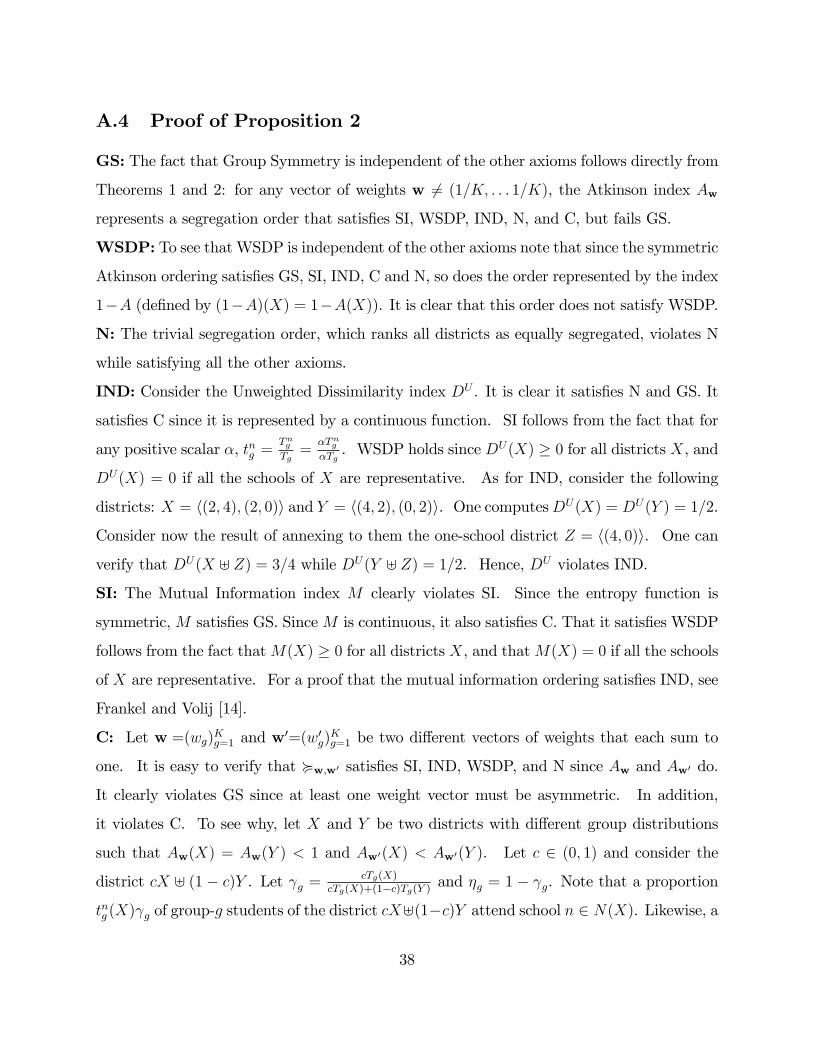
A.4 Proof of Proposition 2
GS: The fact that Group Symmetry is independent of the other axioms follows directly from
Theorems 1 and 2: for any vector of weights w 6= (1=K; : : : 1=K), the Atkinson index Aw
represents a segregation order that satis�es SI, WSDP, IND, N, and C, but fails GS.
WSDP: To see that WSDP is independent of the other axioms note that since the symmetric
Atkinson ordering satis�es GS, SI, IND, C and N, so does the order represented by the index
1�A (de�ned by (1�A)(X) = 1�A(X)). It is clear that this order does not satisfy WSDP.
N: The trivial segregation order, which ranks all districts as equally segregated, violates N
while satisfying all the other axioms.
IND: Consider the Unweighted Dissimilarity index DU . It is clear it satis�es N and GS. It
satis�es C since it is represented by a continuous function. SI follows from the fact that for
any positive scalar �, tng =TngTg=
�Tng�Tg. WSDP holds since DU(X) � 0 for all districts X, and
DU(X) = 0 if all the schools of X are representative. As for IND, consider the following
districts: X = h(2; 4); (2; 0)i and Y = h(4; 2); (0; 2)i. One computesDU(X) = DU(Y ) = 1=2.
Consider now the result of annexing to them the one-school district Z = h(4; 0)i. One can
verify that DU(X ] Z) = 3=4 while DU(Y ] Z) = 1=2. Hence, DU violates IND.
SI: The Mutual Information index M clearly violates SI. Since the entropy function is
symmetric,M satis�es GS. SinceM is continuous, it also satis�es C. That it satis�es WSDP
follows from the fact thatM(X) � 0 for all districts X, and thatM(X) = 0 if all the schools
of X are representative. For a proof that the mutual information ordering satis�es IND, see
Frankel and Volij [14].
C: Let w =(wg)Kg=1 and w0=(w0g)
Kg=1 be two di¤erent vectors of weights that each sum to
one. It is easy to verify that <w;w0 satis�es SI, IND, WSDP, and N since Aw and Aw0 do.
It clearly violates GS since at least one weight vector must be asymmetric. In addition,
it violates C. To see why, let X and Y be two districts with di¤erent group distributions
such that Aw(X) = Aw(Y ) < 1 and Aw0(X) < Aw0(Y ). Let c 2 (0; 1) and consider the
district cX ] (1 � c)Y . Let g =cTg(X)
cTg(X)+(1�c)Tg(Y ) and �g = 1 � g. Note that a proportion
tng (X) g of group-g students of the district cX](1�c)Y attend school n 2 N(X). Likewise, a
38
proportion tng (Y )�g of group-g students of the district cX](1�c)Y attend school n 2 N(Y ).
Therefore, we can write
1� Aw(cX ] (1� c)Y ) =X
n2N(X)
Yg2G
(tng (X) g)wg +
Xn2N(Y )
Yg2G
(tng (Y )�g)wg
=X
n2N(X)
Yg2G
�tng (X)
�wg � g�wg
+X
n2N(Y )
Yg2G
�tng (X)
�wg ��g�wg
=
Yg2G
� g�wg! X
n2N(X)
Yg2G
�tng (X)
�wg+
Yg2G
��g�wg! X
n2N(Y )
Yg2G
�tng (Y )
�wg= (1� Aw(X))
Yg2G
� g�wg
+ (1� Aw(Y ))Yg2G
��g�wg
:
Since the group distributions of X and Y are not the same, there are groups g; g0 2 G with
g 6= g0. (Otherwise, for all groups g, g equals a constant �, which impliesTg(X)
Tg(Y )= �(1�c)
c(1��) .
Hence, X and Y must have the same group distribution, a contradiction.) Therefore, the
geometric averageQg2G
� g�wg is strictly lower than the corresponding arithmetic average,
and the same is true forQg2G
�1� g
�wg . As a result,1� Aw(cX ] (1� c)Y ) < (1� Aw(X))
Xg2G
wg g + (1� Aw(Y ))Xg2G
wg�g:
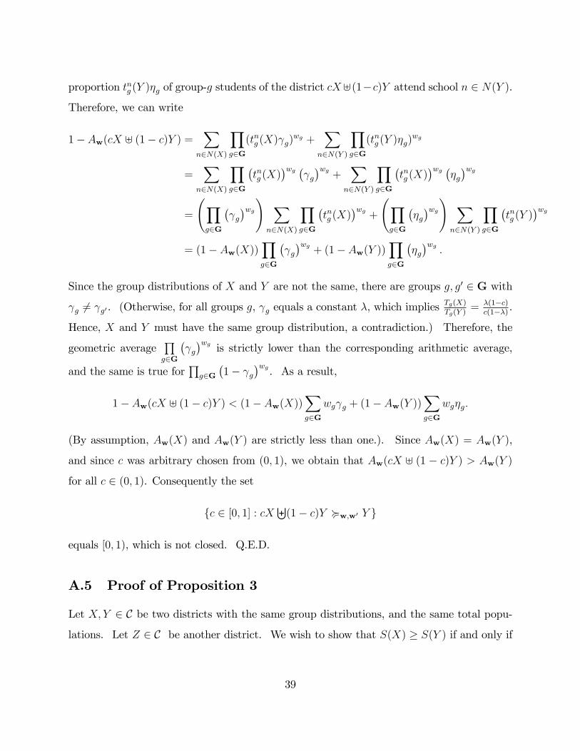
(By assumption, Aw(X) and Aw(Y ) are strictly less than one.). Since Aw(X) = Aw(Y ),
and since c was arbitrary chosen from (0; 1), we obtain that Aw(cX ] (1 � c)Y ) > Aw(Y )
for all c 2 (0; 1). Consequently the set
fc 2 [0; 1] : cXU(1� c)Y <w;w0 Y g
equals [0; 1), which is not closed. Q.E.D.
A.5 Proof of Proposition 3
Let X; Y 2 C be two districts with the same group distributions, and the same total popu-
lations. Let Z 2 C be another district. We wish to show that S(X) � S(Y ) if and only if
39

S(X ] Z) � S(Y ] Z). Note that
S(X ] Z) = S(x ] z) + �(x; z)S(X) + �(x; z)S(Z) by (5)
= S(y ] z) + �(y; z)S(X) + �(y; z)S(Z) since x = y
while S(Y ] Z) = S(y ] z) + �(y; z)S(Y ) + �(y; z)S(Z) by (5). Since �(x; y) > 0 by
assumption, S(X ] Z)� S(Y ] Z) is proportional to S(X)� S(Y ).
40

References
[1] Aczél, J. 1966. �Lectures on Functional Equations and their Applications.�Academic
Press, NewYork and London.
[2] Atkinson, A.B. 1970. �On the Measurement of Inequality.�Journal of Economic Theory
2: 244-63.
[3] Bell, Wendell. 1954. �A Probability Model for the Measurement of Ecological Segre-
gation.� Social Forces 32:357-364.
[4] Boozer, Michael A., Alan B. Krueger, and Shari Wolkin. 1992. �Race and School
Quality Since Brown v. Board of Education.� Brookings Papers on Economic Activity:
Microeconomics 1992, pp. 269-338.
[5] Card, David, and Jesse Rothstein. 2007. �Racial Segregation and the Black-White
Test Score Gap.�Journal of Public Economics 91:2158-2184.
[6] Clotfelter, Charles T. 1979. �Alternative Measures of School Desegregation: AMethod-
ological Note.�Land Economics 54: 373-380.
[7] Clotfelter, Charles T. 1999. �Public School Segregation in Metropolitan Areas.�Land
Economics 75:487-504.
[8] Coleman, James S., Thomas Ho¤er, and Sally Kilgore. 1982. �Achievement and Segre-
gation in Secondary Schools: A Further Look at Public and Private School Di¤erences.�
Sociology of Education 55:162-182.
[9] Cotter, David A., JoAnn DeFiore, Joan M. Hermsen, Brenda M. Kowalewski, and
Reeve Vanneman. 1997. �All Women Bene�t: The Macro-Level E¤ect of Occupational
Integration on Gender Earnings Equality.� American Sociological Review 62:714�734.
[10] Cutler, David, and Edward Glaeser. 1997. �Are Ghettos Good or Bad?�Quarterly
Journal of Economics 112: 827�872.
41

[11] Cutler, David, and Edward Glaeser and Jacob Vigdor. 1999. �The Rise and Decline of
the American Ghetto�Journal of Political Economy 107: 455�506.
[12] Duncan, Otis D., and Beverly Duncan. 1955. �A Methodological Analysis of Segrega-
tion Indices.� American Sociological Review 20:210-217.
[13] Echenique, Federico, and Roland G. Fryer, Jr. 2007. �A Measure of Segregation Based
on Social Interactions.� Quarterly Journal of Economics, 122:441-485.
[14] Frankel, David M., and Oscar Volij. 2007. �Measuring Segregation.�Mimeo.
[15] Guryan, Jonathan. 2005. �Desegregation and Black Dropout Rates.� American Eco-
nomic Review 94:919-943.
[16] Hanushek, Eric A., John F. Kain, and Steven G. Rivkin. 2004. �New Evidence about
Brown v. Board of Education: The Complex E¤ects of School Racial Composition on
Achievement.� NBER Working Paper No. W8741.
[17] Hoxby, Caroline M. 2000. �Peer E¤ects in the Classroom: Learning from Gender and
Race Variation.� NBER Working Paper 7867.
[18] Hutchens, Robert. 2001. �Numerical Measures of Segregation: Desirable Properties
and Their Implications.�Mathematical Social Sciences 42:13�29.
[19] Hutchens, Robert. 2003. �One Measure of Segregation.� International Economic
Review 45:555�578.
[20] Ioannides, Yannis M., and Linda D. Loury. 2004. �Job Information Networks, Neigh-
borhood E¤ects, and Inequality.� Journal of Economic Literature XLII:1056-1093.
[21] Jahn, Julius, and Schmidt, Calvin F., and Schrag, Clarence. 1947. �The Measurement
of Ecological Segregation.�American Sociological Review 12:293�303.
[22] James, David R., and Karl E. Taeuber. 1985. �Measures of Segregation.� Sociological
Methodology 15:1�32.
42

[23] James, Franklin J. 1986. �A New Generalized �Exposure-based�Segregation Index.�
Sociological Methods and Research 14:301-316.
[24] Johnson, Ron, Michael Poulsen, and James Forrest. 2007. Ethnic and Racial Segrega-
tion in U.S. Metropolitan Areas, 1980-2000: The Dimensions of Segregation Revisited.
Urban A¤airs Review 42:479-504.
[25] Lewis, Gregory B. 1996. �Gender Integration of Occupations in the Federal Civil Ser-
vice: Extent and E¤ects on Male-Female Earnings.� Industrial and Labor Relations
Review 49:472�483.
[26] Lieberson, Stanley. 1969. �Measuring Population Diversity.� American Sociological
Review 34:850-862.
[27] Macpherson, David A., and Barry T. Hirsh, 1995. �Wages and Gender Composition:
Why do Women�s jobs Pay Less? � Journal of Labor Economics 13:426�471.
[28] Massey, Douglas S. and Nancy A. Denton. 1988. �The Dimensions of Racial Segrega-
tion.� Social Forces 67:281�315.
[29] McLaughlin, Don. 2003. �CCD Data File: Thirteen-Year Longitudinal Common Core
of Data, Non-Fiscal Survey Database, School Years 1986-87 1998-99.� Mimeo, American
Institutes for Research.
[30] Morgan, Barrie S. 1975. �The Segregation of Socioeconomic Groups in Urban Areas:
A Comparative Analysis.� Urban Studies 12:47-60.
[31] Philipson, Tomas. 1993. �Social Welfare and Measurement of Segregation.� Journal of
Economic Theory 60:322-334.
[32] Reardon, Sean F. 1998. �Measures of Racial Diversity and Segregation in Multigroup
and Hierarchically Structured Populations.� Presented at the Annual Meeting of the
Eastern Sociological Society, Philadelphia, PA.
43

[33] Reardon, Sean F., and Glenn Firebaugh. 2002. �Measures of Multigroup Segregation.�
Sociological Methodology 32:33-67.
[34] Sable, J., Gaviola, N., and Garofano, A. 2007. Documentation to the NCES Common
Core of Data Public Elementary/Secondary School Universe Survey: School Year 200506
(NCES 2007-365). U.S. Department of Education, Washington, D.C.: National Center
for Education Statistics.
[35] Sakoda. J. 1981. �A Generalized Index of Dissimilarity.� Demography 18:245-50.
[36] Shorrocks, A. F. 1980. �The Class of Additively Decomposable Inequality Measures.�
Econometrica 39:613-25.
[37] Shorrocks, A. F. 1984. �Inequality Decompositions by Population Subgroups.�Econo-
metrica 48:1369-86.
[38] Taeuber, Karl E., and David R. James. 1982. �Racial Segregation Among Public and
Private Schools.� Sociology of Education 55:133-143.
[39] Theil, Henri. 1971. �Principles of Econometrics.�Wiley & Sons. New York.
[40] Theil, Henri. 1972. �Statistical Decomposition Analysis.� North Holland.
[41] Theil, Henri., and A. J. Finizza 1971. �A Note on the Measurement of Racial Integration
in Schools.� Journal of Mathematical Sociology 1:187�1193.
[42] Zoloth, Barbara S. 1976. �Alternative Measures of School Segregation.� Land Eco-
nomics 52:278-298.
44

White vs. Black
00.10.20.30.40.50.60.70.80.9
1
0 0.2 0.4 0.6 0.8 1
White vs. Hispanic
00.10.20.30.40.50.60.70.80.9
1
0 0.2 0.4 0.6 0.8 1
White vs. Asian
00.10.20.30.40.50.60.70.80.9
1
0 0.2 0.4 0.6 0.8 1
Black vs. Hispanic
00.10.20.30.40.50.60.70.80.9
1
0 0.2 0.4 0.6 0.8 1
Black vs. Asian
00.10.20.30.40.50.60.70.80.9
1
0 0.2 0.4 0.6 0.8 1
Hispanic vs. Asian
00.10.20.30.40.50.60.70.80.9
1
0 0.2 0.4 0.6 0.8 1
Table 2: Lorenz Curves for Pairs of Ethnic Groups, 1987-8 (thin curve) and 2005-6 (thick curve). Universe is set of U.S.public schools that report positive numbers of students in Common Core of Data for all years from 1987-8 to 2005-6. Schools
are sorted in decreasing order of the ratio of the number students in the �rst group to the number of students in the second
group. As each school is considered in turn, the cumulative proportions of students in each group are plotted. The �rst group
appears on the horizontal axis; the second group, on the vertical axis.
45

1987/88 2005/06 Change1. PAIRWISE GINI COEFFICIENTS
WhiteBlack 0.851 0.846 0.005WhiteHispanic 0.899 0.861 0.038WhiteAsian 0.791 0.760 0.031BlackHispanic 0.918 0.854 0.064BlackAsian 0.910 0.872 0.038HispanicAsian 0.846 0.803 0.043
2. PUBLIC SCHOOL ETHNIC DISTRIBUTIONAsians 4.0% 5.7% 1.7%Whites 70.8% 58.2% 12.6%Blacks 15.3% 16.8% 1.5%Hispanics 10.0% 19.3% 9.3%TOTAL 100.0% 100.0% 0.0%
3. SCALE INVARIANT INDICESUIOD (Unweighted Dissimilarity) 0.639 0.599 0.040ATKSYM (Asymmetric Atkinson) 0.640 0.528 0.112ATK05 (Atkinson; 2005/06 weights) 0.614 0.472 0.142ATK87 (Atkinson; 1987/88 weights) 0.573 0.406 0.167
4. UNNORMALIZED SCALEVARIANT INDICESM (Mutual Information) 0.586 0.679 0.093Cl50 (Clotfelter with 50% threshold) 0.572 0.681 0.108Cl90 (Clotfelter with 90% threshold) 0.268 0.325 0.057CR (CardRothstein) 0.461 0.482 0.021
5. NORMALIZED SCALEVARIANT INDICESGINI 0.818 0.793 0.024WIOD (Weighted Dissimilarity) 0.648 0.624 0.024NEXP (Normalized Exposure) 0.440 0.446 0.006ENT (Entropy Segregation Index) 0.456 0.429 0.027
6. MISCELLANEOUSD' (Unnormalized Dissimilarity) 0.301 0.370 0.069G' (Unnormalized GINI) 0.380 0.470 0.091I (Simpson Interaction Index) 0.464 0.593 0.129h(P) (Entropy of US Ethnic Distribution) 1.285 1.582 0.297Number of Schools 62519 62519 0.000Number of Students (millions) 33.29 34.08 0.796
School Year
Table 3: Summary Statistics for U.S. Public Schools, 1987/8 and 2005/6. Universe is set of
U.S. public schools that report positive numbers of students in Common Core of Data for
all school years from 1987/8 to 2005/6.
46


![Chapter IX Measures on Fractals - Imperial College Londonjswlamb/M345PA46/[B] chap IX.pdf · Chapter IX Measures on Fractals 1 Introduction to Invariant Measures on Fractals 330 In](https://img.pdfslide.us/doc/110x75/5f12d2e0092d717fef192f35/chapter-ix-measures-on-fractals-imperial-college-jswlambm345pa46b-chap-ixpdf.jpg)