Scale-Free Coordinates forMulti-Robot Systems withBearing-only Sensors

Alejandro Cornejo, Andrew J. Lynch, Elizabeth FudgeSiegfried Bilstein, Majid Khabbazian, James McLurkin

Abstract We propose scale-free coordinates as an alternative coordinate sys-tem for multi-robot systems with large robot populations. Scale-free coor-dinates allow each robot to know, up to scaling, the relative position andorientation of other robots in the network. We consider a weak sensing modelwhere each robot is only capable of measuring the angle, relative to its ownheading, to each of its neighbors. Our contributions are three-fold. First,we derive a precise mathematical characterization of the computability ofscale-free coordinates using only bearing measurements, and we describe anefficient algorithm to obtain them. Second, through simulations we show thateven in graphs with low average vertex degree, most robots are able to com-pute the scale-free coordinates of their neighbors using only 2-hop bearingmeasurements. Finally, we present an algorithm to compute scale-free co-ordinates that is tailored to low-cost systems with limited communicationbandwidth and sensor resolution. Our algorithm mitigates the impact of sens-ing errors through a simple yet effective noise sensitivity model. We validateour implementation with real-world robot experiments using static accuracymeasurements and a simple scale-free motion controller.

1 IntroductionLarge populations of robots can solve many challenging problems such as

mapping, exploration, search-and-rescue, and surveillance. All these appli-cations require robots to have at least some information about the networkgeometry : knowledge about other robots positions and orientations relativeto their own [1]. Different approaches to computing network geometry havetrade-offs between the amount of information recovered, the complexity ofthe sensors, the amount of communications required and the cost. A GPSsystem provides each robot with a global position, which can be used toderive complete network geometry, but GPS is not available in many envi-ronments: indoors, underwater, or on other planets. The cost and complexityof most vision- and SLAM-based approaches makes them unsuitable for largepopulations of simple robots.

This work proposes scale-free coordinates as a slightly weaker alternative tothe complete network geometry. We argue that scale-free coordinates provide

1

2 Cornejo et. al.

sufficient information to perform many canonical multi-robot applications,while still being implementable using a weak sensing platform. Informally,scale-free coordinates provide the complete network geometry informationup to an unknown scaling factor i.e. the robots can recover the shape of thenetwork, but not its scale.

Formally, the scale-free coordinates of a set of robots S is described bya set of tuples {(xi, yi, θi) | i ∈ S}. The relative position of robot i ∈ S isrepresented by the coordinates (xi, yi) which match are correct up to thesame (but unknown) multiplicative constant α. The relative orientation ofrobot i ∈ S is represented by θi. Of particular interest to us are the localscale-free coordinates of a robot, which are simply the scale-free coordinatesof itself and its neighbors, measured from its reference frame.

We consider a simple sensing model in which each robot can only measurethe angle, relative to its own heading, to neighboring robots. These sensors areappropriate for low-cost robots that can be deployed in large populations [2].Our approach allows each robot to use the bearing measurements available inthe network to determine the relative positions and orientations of any subsetof robots up to scaling. We remark that in this work we make no assumptionson the relationship between the Euclidean distance between two robots andpresence of an edge in the communication graph between them. In particular,we do not assume the communication graph is a unit disk graph, or any othertype of geometric graph.

Fig. 1: Two distinct Voronoi cells with thesame angle measurements. A robot cannotdistinguish these cells using only the anglemeasurements to its neighbors.

With only local bearing measure-ments, a robot has the capabilityto execute a large number of algo-rithms [3, 4, 5], but this informa-tion is insufficient to directly com-pute all the parameters of its net-work geometry. For instance, con-sider the canonical problem of con-trolling a multi-robot system to acentroidal Voronoi configuration [6].This is straightforward to solve withthe complete network geometry, butit is not possible to using only the bearing measurements to your neighbors.Figure 1 shows two configurations with the same bearing measurements thatproduce very different Voronoi cells (in this diagram we assume robots at thecenter of adjacent Voronoi cells are neighbors in the communication graph).Local scale-free coordinates are sufficient for each robot to compute the shapeof its Voronoi cell. However, since scale-free distances have no units, therobot cannot distinguish between 3 m or 3 cm distance to the centroid. Thispresents challenges to algorithms, in particular to motion control, which weconsider in our experiments in Section 5.3.

There are three main contributions in this work. Section 3 presents thetheoretical foundation for scale-free coordinates, and proves the necessaryand sufficient conditions required to compute scale-free coordinates for theentire configuration of robots. We then generalize this approach to computethe scale-free coordinates of any subset of the robots. Section 4 shows throughsimulations, that in random configurations most robots are able to computetheir local scale-free coordinates in only 3 or 4 communication rounds, even

Scale-Free Coordinates for Multi-Robot Systems 3

in in networks with low average degree. Section 5 presents a simplified al-gorithm, tailored for our low-cost multi-robot platform [7], to compute localscale-free coordinates using information from the 2-hop neighborhood aroundeach robot. The 2-hop algorithm computes scale-free coordinates efficientlywith a running time that is linear in the number of angle measurements. Ourplatform is equipped with sensors that only measure coarse bearing to neigh-boring robots, we mitigate the effect of this errors through a noise sensitivitymodel. We show accuracy data from static configurations, and implementa simple controller to demonstrate the feasibility of using the technique formotion control.

1.1 Related WorkMuch of the previous work on computation of coordinates for multi-robot

systems focuses on computing coordinates for each robot using beacon oranchor robots (or landmarks) with known coordinates [8, 9, 10]. There arealso distributed approaches, which do not require globally accessible bea-con robots, but instead use multi-hop communication to spread the beaconpositions throughout the network [11]. Generally, these approaches do notscale for large swarms of simple mobile robots. Moreover, these approachesare generally based on some form of triangulation. In contrast, the approachproposed in this paper can be used to compute the scale-free coordinates evenin graphs where there does not exist a single triangle.

The literature presents multiple approaches to network geometry suchas pose in a shared external reference frame [12], pose in a local referenceframe [1], distance-only [13, 14, 15] bearing-only [16, 17, 18], sorted order ofbearing [19], or combinatorial visibility [20].

The closest in spirit to our work is the “robust quads” work of Mooreet. al. [13]. Using inter-robot distance information, they find robust quadri-laterals in the network around each robot and combine them to recover thepositions of the robot’s neighbors. Our work is in the same vein, except thatwe use inter-robot bearing information instead, which allows us to also re-cover relative orientation. In the error-free case, we present localization suc-cess rates which are comparable to the Moore results. However, our approachhas less requirements on the graph; scale-free coordinates can be extracted ina graph formed by robust quadrilaterals, but there are graphs without evena single robust quadrilateral where scale-free coordinates are computable.

From the computational geometry literature, the closest work to ours itthat of Whiteley [21], who studied directional graph rigidity using the toolsof matroid theory. This paper follows a simpler alternative algebraic charac-terization that allows us to directly compute the scale-free coordinates of anysubset of robots. In addition, Bruck [22] addresses the problem of finding aplanar spanner of a unit disk graph by only using local angles. The Bruckwork is similar to our approach of forming a virtual coordinate system, buttheir focus delves into routing schemes for sensor networks.

Bearing-only models are more limited than range-bearing models and thetype of problems to solve is reduced. In addition, the amount of inter-robotcommunication often increases greatly. The inter-robot communication re-quirement is often overlooked in the literature. However, algorithms that re-quire large amounts of information from neighboring robots or many roundsof message passing are impractical on systems with limited bandwidth. This

4 Cornejo et. al.

work uses the bearing-only sensor model with scale-free coordinates to bal-ance the trade-off between cost, complexity, communications, and capability.

2 System Model and DefinitionsWe assume each robot is deployed at an arbitrary position in the Euclidean

plane and with an arbitrary orientation unit vector. The communication net-work is modeled as an undirected graph, G = (V,E), where every vertexin the graph represents a robot, and N(u) = {v | {u, v} ∈ E} denotes theneighbors of robot u. We consider a synchronous network model, where theexecution progresses in synchronous lock-step rounds. During each round ev-ery robot can send a message to its neighbors, and receive any messagessent to it by its neighbors. Moreover we assume that when node u receives amessage from node v, it also measures the angle θ(u, v), relative to its ownorientation, from u to v. These assumption greatly simplifies the analysis,and can be implemented easily in a physical system via synchronizers [1].

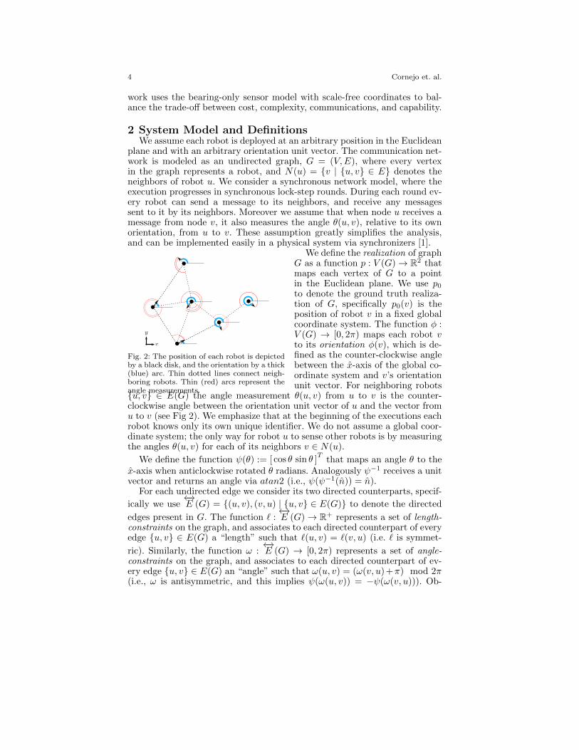
Fig. 2: The position of each robot is depictedby a black disk, and the orientation by a thick(blue) arc. Thin dotted lines connect neigh-boring robots. Thin (red) arcs represent theangle measurements.

We define the realization of graphG as a function p : V (G)→ R2 thatmaps each vertex of G to a pointin the Euclidean plane. We use p0to denote the ground truth realiza-tion of G, specifically p0(v) is theposition of robot v in a fixed globalcoordinate system. The function φ :V (G) → [0, 2π) maps each robot vto its orientation φ(v), which is de-fined as the counter-clockwise anglebetween the x̂-axis of the global co-ordinate system and v’s orientationunit vector. For neighboring robots

{u, v} ∈ E(G) the angle measurement θ(u, v) from u to v is the counter-clockwise angle between the orientation unit vector of u and the vector fromu to v (see Fig 2). We emphasize that at the beginning of the executions eachrobot knows only its own unique identifier. We do not assume a global coor-dinate system; the only way for robot u to sense other robots is by measuringthe angles θ(u, v) for each of its neighbors v ∈ N(u).

We define the function ψ(θ) := [ cos θ sin θ ]T

that maps an angle θ to thex̂-axis when anticlockwise rotated θ radians. Analogously ψ−1 receives a unitvector and returns an angle via atan2 (i.e., ψ(ψ−1(n̂)) = n̂).

For each undirected edge we consider its two directed counterparts, specif-

ically we use←→E (G) = {(u, v), (v, u) | {u, v} ∈ E(G)} to denote the directed

edges present in G. The function ` :←→E (G)→ R+ represents a set of length-

constraints on the graph, and associates to each directed counterpart of everyedge {u, v} ∈ E(G) a “length” such that `(u, v) = `(v, u) (i.e. ` is symmet-

ric). Similarly, the function ω :←→E (G) → [0, 2π) represents a set of angle-

constraints on the graph, and associates to each directed counterpart of ev-ery edge {u, v} ∈ E(G) an “angle” such that ω(u, v) = (ω(v, u)+π) mod 2π(i.e., ω is antisymmetric, and this implies ψ(ω(u, v)) = −ψ(ω(v, u))). Ob-

Scale-Free Coordinates for Multi-Robot Systems 5

serve that if all the robots had the same orientation then the set of all anglemeasurements would describe a set of angle-constraints on G.

We say p is a satisfying realization of (G, `) iff every edge (u, v) ∈←→E (G)

satisfies ‖p(v)− p(u)‖ = `(u, v). Realizations are length-equivalent if onecan be obtained from the other by a translation, rotation or reflection(distances are invariant to these operations). A length-constrained graph(G, `) has a unique realization if all its satisfying realizations are length-equivalent. Similarly, we say p is a satisfying realization of (G,ω) iff every

edge (u, v) ∈←→E (G) satisfies p(v) − p(u) = ψ(ω(u, v)) ‖p(v)− p(u)‖. Re-

alizations are angle-equivalent if one can be obtained from the other by atranslation or uniform-scaling (angles are invariant to these operations). Anangle-constrained graph (G,ω) has a unique realization if all its satisfyingrealizations are angle-equivalent.

3 Theoretical Foundation for Scale-Free CoordinatesThis section develops a mathematical framework that characterizes the

computability of scale-free coordinates and outlines an efficient procedure tocompute them. The full procedure derivation with proofs appears in a tech re-port [23]. Here we omit some intermediate results and present a self-containedsummary. First all the robots in the network to agree on a common referenceorientation. In a connected graph this is accomplished by having each robotpropagating orientation offsets to the entire network with a broadcast tree.As a side-effect of this procedure every robot can compute the relative orien-tation of every other robot. The details of this distributed algorithm, alongwith proofs of correctness, appear in [23]. In the rest of the paper we assumethat all angle measurements are taken with respect to a global x̂-axis andtherefore constitute a valid set of angle-constraints on the graph.

Given an angle-constrained graph, the task of computing scale-free coor-dinates for every robot is equivalent to finding a unique satisfying realizationof the graph. If such a realization does not exist, then either there is no set ofscale-free coordinates consistent with the angle-measurements, (perhaps dueto measurement errors), or there are multiple distinct sets of scale-free coor-dinates which produce the same angle measurements, and it is impossible toknow which one of them corresponds to the ground truth. We note that everyrealization of a graph induces a unique set of length- and angle-constraintswhich are simultaneously satisfied by that realization:

Proposition 1. A realization p of a graph G induces a unique set of length-and angle-constraints `p and ωp which are simultaneously satisfied by p.

However, the converse does not hold, since there are length- and angle-constraints that do not have a realization which satisfies them simultaneously.

The necessary and sufficient conditions that determine if a set of angle-constraints have a satisfying realization are captured by the cycles of thegraph. In particular, given any realization p of G, traversing a directed cycleC of G and returning to the starting vertex there will be no net change inposition or orientation. Formally:

6 Cornejo et. al.∑(u,v)∈E(C)

(p(v)− p(u)) =∑

(u,v)∈E(C)

`p(u, v)ψ(ωp(u, v)) = 0. (1)

Since by definition `p(u, v) = `p(v, u) and ψ(ωp(u, v)) = −ψ(ωp(v, u)) wecan verify that the direction in which we traverse an undirected cycle is notrelevant, since both directions produce the same equation. Since the termsof the equations are two-dimensional vectors, each cycle generates two scalarequations for the x- and y-component. If the realization p of G is unknown,but we know both G and a set of angle-constraints ω of G, then equation 1represents two linear restrictions on the length of the edges of any realizationp which satisfies (G,ω).

The number of cycles in a graph can be exponential, however we showit suffices to consider only the cycles in a cycle basis of G. For a detaileddefinition of a cycle basis we refer the interested reader to [24]. Briefly, acycle basis of a graph is a subset of the simple undirected cycles presentin a graph, and a connected graph on n vertices and m edges has a cyclebasis with exactly m − n + 1 cycles. A cycle basis of G can be constructedin O(m · n) time by first constructing a spanning tree T of G. This leavesm − n + 1 non-tree edges, each of which forms a unique simple cycle whenadded to T . Let C = {C1, . . . , Cq} be any cycle basis of G.

It will be useful to represent the length of the edges of a realization as areal vector. Let E = {e1, . . . , em} be any ordered set of directed edges thatcover all the undirected edges in E(G). Specifically for every undirected edgein E(G) one of its directed counterparts (but not both) is present in E(G),conversely if a directed edge is present in E(G) then its undirected versionis in E(G). Let x be an m× 1 column vector whose ith entry represents thelength of the directed edge ei ∈ E of any satisfying realization of (G,ω).

Applying equation 1 to a cycle basis of G results in the following:

e1 · · · emC1

...Cq

a11 . . . a1m...

. . ....

aq1 . . . aqm

︸ ︷︷ ︸

A(G,ω)

`p(e1)...

`p(em)

︸ ︷︷ ︸

x

= 0. (2)

Here A(G,ω) is a 2q × m matrix constructed using G, C and ω. Row icorresponds to a cycle Ci ∈ C , and column j corresponds to an edge(u, v) ∈ E . If (u, v) ∈ E(Ci) then aij = ψ(ω(u, v)), if (v, u) ∈ E(Ci) thenaij = −ψ(ω(u, v)) = ψ(ω(v, u)), otherwise aij = 0. Since these are vectorequations, there are two scalar rows in A(G,ω) for every cycle in C – oneequation for the x-components and one for the y-components of each cycle.

Equation 2 is a homogeneous system, therefore the solution space is pre-cisely the null space of A(G,ω), denoted by null(A(G,ω)). Our main result re-lates the null space of A(G,ω) to the space of satisfying realizations of (G,ω).

Let P(G,ω) be a set of realizations that satisfy (G,ω), where all equivalentrealizations are mapped to a single realization that “represents” its equiva-lence class. We define the function fω : P(G,ω) → Rm that maps a realizationin P(G,ω) to a (positive) m-dimensional real vector which contains in its ith en-try the length of the directed edge ei ∈ E . Therefore fω(p) is simply a vector

Scale-Free Coordinates for Multi-Robot Systems 7

representation of the set of length-constraints `p satisfied by p. Observe thatproposition 1 implies that when the domain of fω is restricted to P(G,ω) then

fω has an inverse f−1ω . We now state the main theorem of this section:

Theorem 2. p ∈ P(G,ω) if and only if fω(p) ∈ null(A(G,ω)).

This theorem implies each column in the null space basis of A(G,ω) corre-sponds to a distinct satisfying realization of (G,ω), and therefore a distinctset of scale-free coordinates. If the nullity of A(G,ω), the number of columnsof its null space basis, is zero no set of scale-free coordinates is consistentwith the angle-measurements. If the nullity is one, then there is a single setof scale-free coordinates which are consistent with the angle-measurements.If on the other hand the nullity of A(G,ω) is greater than one, then there aremultiple distinct sets of scale-free coordinates consistent with the angle mea-surements and its impossible to know which one corresponds to the groundtruth. We summarize this in the following corollary.

Corollary 1. (G,ω) has a unique satisfying realization ⇐⇒ the nullityof A(G,ω) is one ⇐⇒ the scale-free coordinates of every robot in G arecomputable.

3.1 Local Scale-Free CoordinatesThis subsection describes a procedure that uses the null space basis of

A(G,ω) to compute the scale-free coordinates of any subset of robots. Ofparticular interest to us is computing the scale-free coordinate of a specificrobot and its neighbors (i.e., its local scale-free coordinates). From corollary 1it follows that if the null space basis of A(G,ω) has a single column, thenwe can compute the scale-free coordinates of any subset of robots, since wecan compute scale-free coordinates for all robots simultaneously. However,it might be the case that the null space basis of A(G,ω) has more than onecolumn, but it is still possible to compute the scale-free coordinates of somesubset of the robots.

For a set S ⊆ V (G) of vertices, let G[S] be the subgraph of G induced by S,and let `[S] and ω[S] be the length- and angle-constraints that correspond tothe edges in G[S]. We say an angle-constrained (G,ω) has a unique S-subsetrealization iff when restricted to the vertices of S all realizations of (G,ω)projected to the vertices in S are equivalent. From this definition we can seethat the scale-free coordinates of the subset of robots in S are computableiff (G,ω) has a unique S-subset realization. Using these definitions we canprove the following.

Lemma 3. The angle-constrained graph (G,ω) has a unique S-subset real-ization iff there is a superset S′ ⊇ S such that (G[S′], ω[S′]) has a uniquerealization.

The FixedTree algorithm leverages this lemma to compute scale-freecoordinates for any subset of robots. The FixedTree algorithm receives asinput a graph G, a subset of vertices S ⊆ V (G), and a null space basis N ofA(G,ω). If there exists a superset S′ ⊇ S such that (G[S′], ω[S′]) has a uniquerealization it will return this set. From corollary 1 it follows that we canuse this set S′ and the null space basis N to compute the unique satisfyingrealization, and therefore the scale-free coordinates, of S′ ⊇ S.

8 Cornejo et. al.

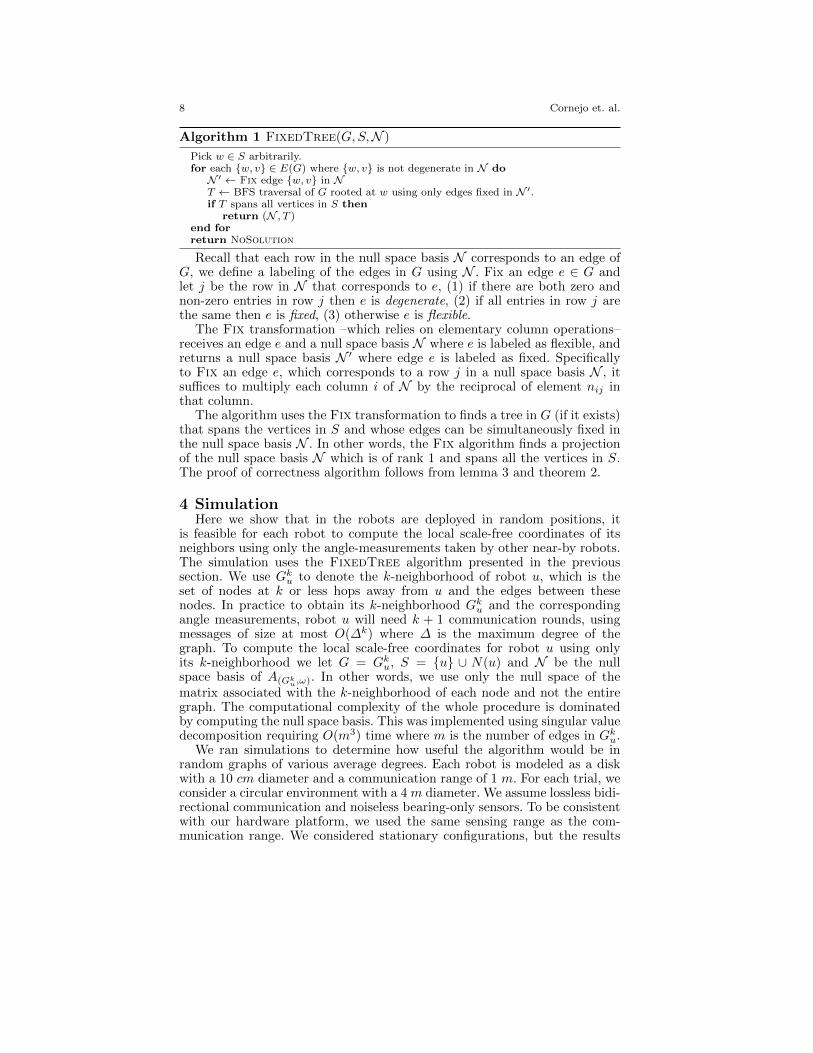
Algorithm 1 FixedTree(G,S,N )

Pick w ∈ S arbitrarily.for each {w, v} ∈ E(G) where {w, v} is not degenerate in N doN ′ ← Fix edge {w, v} in NT ← BFS traversal of G rooted at w using only edges fixed in N ′.if T spans all vertices in S then

return (N , T )end forreturn NoSolution

Recall that each row in the null space basis N corresponds to an edge ofG, we define a labeling of the edges in G using N . Fix an edge e ∈ G andlet j be the row in N that corresponds to e, (1) if there are both zero andnon-zero entries in row j then e is degenerate, (2) if all entries in row j arethe same then e is fixed, (3) otherwise e is flexible.

The Fix transformation –which relies on elementary column operations–receives an edge e and a null space basis N where e is labeled as flexible, andreturns a null space basis N ′ where edge e is labeled as fixed. Specificallyto Fix an edge e, which corresponds to a row j in a null space basis N , itsuffices to multiply each column i of N by the reciprocal of element nij inthat column.

The algorithm uses the Fix transformation to finds a tree in G (if it exists)that spans the vertices in S and whose edges can be simultaneously fixed inthe null space basis N . In other words, the Fix algorithm finds a projectionof the null space basis N which is of rank 1 and spans all the vertices in S.The proof of correctness algorithm follows from lemma 3 and theorem 2.

4 SimulationHere we show that in the robots are deployed in random positions, it

is feasible for each robot to compute the local scale-free coordinates of itsneighbors using only the angle-measurements taken by other near-by robots.The simulation uses the FixedTree algorithm presented in the previoussection. We use Gk

u to denote the k-neighborhood of robot u, which is theset of nodes at k or less hops away from u and the edges between thesenodes. In practice to obtain its k-neighborhood Gk

u and the correspondingangle measurements, robot u will need k + 1 communication rounds, usingmessages of size at most O(∆k) where ∆ is the maximum degree of thegraph. To compute the local scale-free coordinates for robot u using onlyits k-neighborhood we let G = Gk

u, S = {u} ∪ N(u) and N be the nullspace basis of A(Gk

u,ω). In other words, we use only the null space of thematrix associated with the k-neighborhood of each node and not the entiregraph. The computational complexity of the whole procedure is dominatedby computing the null space basis. This was implemented using singular valuedecomposition requiring O(m3) time where m is the number of edges in Gk

u.We ran simulations to determine how useful the algorithm would be in

random graphs of various average degrees. Each robot is modeled as a diskwith a 10 cm diameter and a communication range of 1 m. For each trial, weconsider a circular environment with a 4 m diameter. We assume lossless bidi-rectional communication and noiseless bearing-only sensors. To be consistentwith our hardware platform, we used the same sensing range as the com-munication range. We considered stationary configurations, but the results

Scale-Free Coordinates for Multi-Robot Systems 9

3 4 5 6 7 8 9 10 110

0.1

0.2

0.3

0.4

0.5

0.6

0.7

0.8

0.9

1Percent of Rigid Robots vs. Average Degree of Graph

Average Degree of Graph

Perc

ent o

f Rig

id R

obot

s

k = 1k = 2k = 3k = 4k = 1 MWAk = 2 MWAk = 3 MWAk = 4 MWA

(a) All Graphs

3 4 5 6 7 8 9 10 110

0.1

0.2

0.3

0.4

0.5

0.6

0.7

0.8

0.9

1

Average Degree of Graph

Perc

ent o

f Rig

id R

obot

s

Percent of Rigid Robots (k = 1)

k = 1k = 1 MWA

(b) Data for k = 1

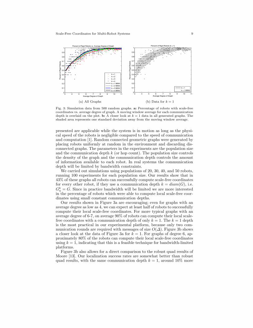
Fig. 3: Simulation data from 500 random graphs. a: Percentage of robots with scale-freecoordinates vs. average degree of graph. A moving window average for each communicationdepth is overlaid on the plot. b: A closer look at k = 1 data in all generated graphs. Theshaded area represents one standard deviation away from the moving window average.

presented are applicable while the system is in motion as long as the physi-cal speed of the robots is negligible compared to the speed of communicationand computation [1]. Random connected geometric graphs were generated byplacing robots uniformly at random in the environment and discarding dis-connected graphs. The parameters in the experiments are the population sizeand the communication depth k (or hop count). The population size controlsthe density of the graph and the communication depth controls the amountof information available to each robot. In real systems the communicationdepth will be limited by bandwidth constraints.

We carried out simulations using populations of 20, 30, 40, and 50 robots,running 100 experiments for each population size. Our results show that in43% of these graphs all robots can successfully compute scale-free coordinatesfor every other robot, if they use a communication depth k = diam(G), i.e.Gk

u = G. Since in practice bandwidth will be limited we are more interestedin the percentage of robots which were able to compute local scale-free coor-dinates using small constant communication depths.

Our results shown in Figure 3a are encouraging; even for graphs with anaverage degree as low as 4, we can expect at least half of robots to successfullycompute their local scale-free coordinates. For more typical graphs with anaverage degree of 6-7, on average 90% of robots can compute their local scale-free coordinates with a communication depth of only k = 1. The k = 1 depthis the most practical in our experimental platform, because only two com-munication rounds are required with messages of size O(∆). Figure 3b showsa closer look at the data of Figure 3a for k = 1. For graphs of degree 6, ap-proximately 80% of the robots can compute their local scale-free coordinatesusing k = 1, indicating that this is a feasible technique for bandwidth-limitedplatforms.

Figure 3b also allows for a direct comparison to the robust quad results ofMoore [13]. Our localization success rates are somewhat better than robustquad results, with the same communication depth k = 1, around 10% more

10 Cornejo et. al.

(a) r-one robot (b) IR regions (c) APRIL tags

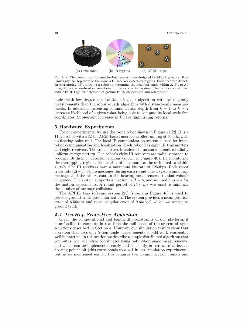
Fig. 4: a: The r-one robot for multi-robot research was designed by MRSL group at RiceUniversity. b: Top view of the r-one’s IR receiver detection regions. Each receiver detectsan overlapping 68◦, allowing a robot to determine the neighbor angle within 22.5◦. c: Animage from the overhead camera from our data collection system. The robots are outfittedwith APRIL tags for detection of ground-truth 2D position and orientation.

nodes with low degree can localize using our algorithm with bearing-onlymeasurements than the robust-quads algorithm with distance-only measure-ments. In addition, increasing communication depth from k = 1 to k = 2increases likelihood of a given robot being able to compute its local scale-freecoordinates. Subsequent increases in k have diminishing returns.

5 Hardware ExperimentsFor our experiments, we use the r-one robot shown in Figure 4a [2]. It is a

11 cm robot with a 32-bit ARM-based microcontroller running at 50 mhz withno floating point unit. The local IR communication system is used for inter-robot communication and localization. Each robot has eight IR transmittersand eight receivers. The transmitters broadcast in unison and emit a radiallyuniform energy pattern. The robot’s eight IR receivers are radially spaced toproduce 16 distinct detection regions (shown in Figure 4b). By monitoringthe overlapping regions, the bearing of neighbors can be estimated to within≈ π/8. The IR receivers have a maximum bit rate of 1250bps. Each robottransmits (∆+1) 4-byte messages during each round, one a system announcemessage, and the others contain the bearing measurements to that robot’sneighbors. The system supports a maximum ∆ = 8, and we used a ∆ = 4 forthe motion experiments. A round period of 2500 ms was used to minimizethe number of message collisions.

The APRIL tags software system [25] (shown in Figure 4c) is used toprovide ground-truth pose information. The system provides a mean positionerror of 6.56mm and mean angular error of 9.6mrad, which we accept asground truth.

5.1 TwoHop Scale-Free AlgorithmGiven the computational and bandwidth constraints of our platform, it

is unfeasible to compute in real-time the null space of the system of cycleequations described in Section 4. However, our simulation results show thata system that uses only 2-hop angle measurements should work reasonablywell in practice. In this section we describe a simple distributed algorithm thatcomputes local scale-free coordinates using only 2-hop angle measurements,and which can be implemented easily and efficiently in hardware without afloating point unit (this corresponds to k = 1 in our simulation experiments,but as we mentioned earlier, this requires two communication rounds and

Scale-Free Coordinates for Multi-Robot Systems 11

angle measurements from 2-hops, hence the name). Later we describe how tomodify the algorithm to deal with sensing errors.

The main insight behind our algorithm is that instead of considering anarbitrary cycle-basis, when restricted to a 2-hop neighborhood of u we canalways restrict ourselves to a cycle-basis composed solely of triangles of whichnode u is a part of. This is a consequence of the following lemma.

Theorem 4. Robot u can compute its local scale-free coordinates using 2-hopangle measurements if and only if the graph induced by the vertices in N(u)is connected.

The basic idea behind the TwoHop Scale-Free algorithm is to traversea tree of triangles, computing the lengths of the edges of the triangles usingthe SineLaw . Specifically, SineLaw receives a triangle (u, z, w) in in the2-hop neighborhood of u. It assumes the length `z of the edge (u, z) is known(up to scale), and uses the inner angles ψz = θ(z, u) − θ(z, w) and ψw =θ(w, z)− θ(w, u) to return the length (up to scale) of edge (u, v).

SineLaw(u, z, w) = `z

∣∣∣∣ sin(θ(z, u)− θ(z, w))

sin(θ(w, z)− θ(w, u))

∣∣∣∣The following algorithm has a running time which is linear in the number

of angle measurements in the 2-hop neighborhood of u.

Algorithm 2 TwoHop Scale-Free algorithm running at node u

1: Fix v ∈ N(u)2: mark v and set `v ← 13: Q← queue(v)4: while Q 6= ∅ do5: z ← Q.pop()6: for each unmarked w ∈ N(z) ∩N(u) do7: mark w and set `w ← SineLaw (u, z, w)8: Q.push(w)9: end for

10: end while

Noise Sensitivity. To deal with coarse sensor measurements while preserv-ing the computational efficiency (and simplicity) of the algorithm we intro-duce the concept of noise sensitivity. Informally, the noise sensitivity of atriangle captures the expected error of the lengths of a triangle when its an-gles are subject to small changes. For example, observe that given a triangle(u, v, z), as ψz gets closer to zero, the output of the SineLaw becomes more“sensitive to noise”, since a small change in the angle measurements usedto compute ψz translate to a potentially very large change in the computedlength. Formally, the noise sensitivity of each triangle can be defined as afunction of the magnitude of the vector gradient of SineLaw(u, v, z). Thisprovides us with an approximation of the expected error in the computedlength when using a particular triangle.

Hence, to reduce the effect of noisy measurements in the computed scale-free coordinates it suffices to find a spanning tree of triangles that has thesmallest total noise sensitivity. This can be achieved by any standard min-imum spanning tree algorithm at minimal additional computational cost.Specifically in our setting a minimum spanning tree of triangles can be found

12 Cornejo et. al.

(a) (b) (c) (d)

0 20 40 60 80 1000

5

10

15

20

25

30

Numb

er of

Sam

ples

Edge Error %

Static Error−UnweightedStatic Error−Weighted

(e)

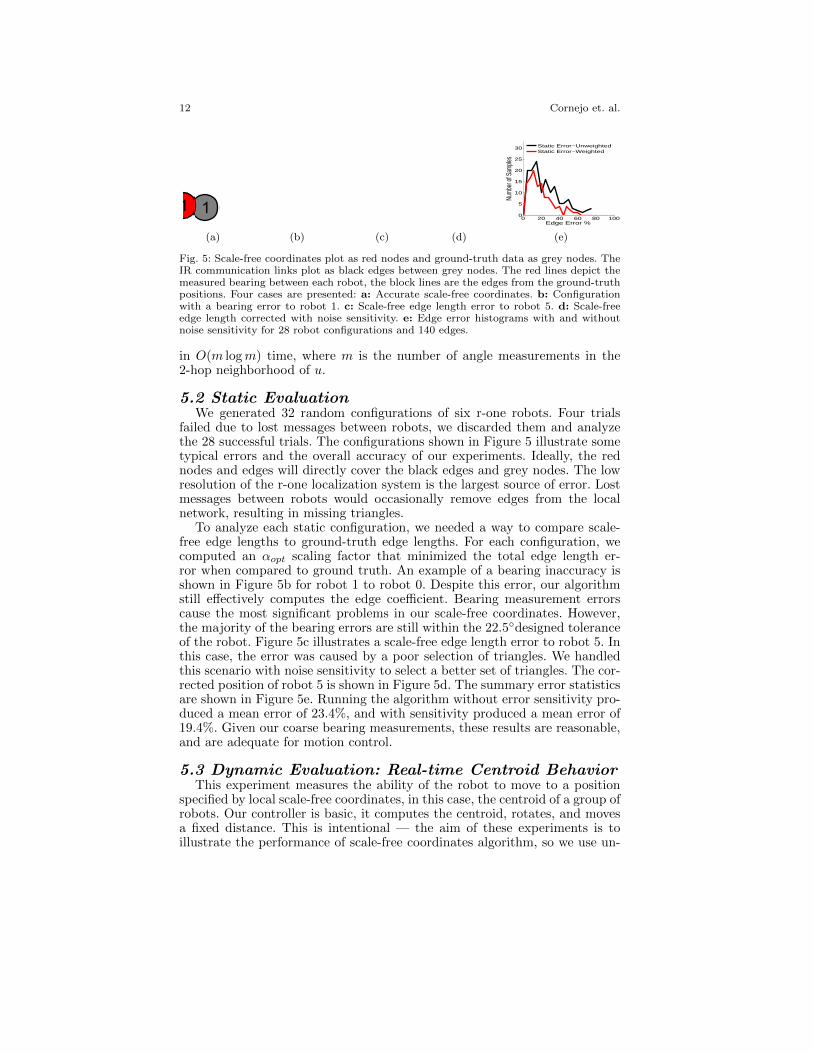
Fig. 5: Scale-free coordinates plot as red nodes and ground-truth data as grey nodes. TheIR communication links plot as black edges between grey nodes. The red lines depict themeasured bearing between each robot, the block lines are the edges from the ground-truthpositions. Four cases are presented: a: Accurate scale-free coordinates. b: Configurationwith a bearing error to robot 1. c: Scale-free edge length error to robot 5. d: Scale-freeedge length corrected with noise sensitivity. e: Edge error histograms with and withoutnoise sensitivity for 28 robot configurations and 140 edges.

in O(m logm) time, where m is the number of angle measurements in the2-hop neighborhood of u.

5.2 Static EvaluationWe generated 32 random configurations of six r-one robots. Four trials

failed due to lost messages between robots, we discarded them and analyzethe 28 successful trials. The configurations shown in Figure 5 illustrate sometypical errors and the overall accuracy of our experiments. Ideally, the rednodes and edges will directly cover the black edges and grey nodes. The lowresolution of the r-one localization system is the largest source of error. Lostmessages between robots would occasionally remove edges from the localnetwork, resulting in missing triangles.

To analyze each static configuration, we needed a way to compare scale-free edge lengths to ground-truth edge lengths. For each configuration, wecomputed an αopt scaling factor that minimized the total edge length er-ror when compared to ground truth. An example of a bearing inaccuracy isshown in Figure 5b for robot 1 to robot 0. Despite this error, our algorithmstill effectively computes the edge coefficient. Bearing measurement errorscause the most significant problems in our scale-free coordinates. However,the majority of the bearing errors are still within the 22.5◦designed toleranceof the robot. Figure 5c illustrates a scale-free edge length error to robot 5. Inthis case, the error was caused by a poor selection of triangles. We handledthis scenario with noise sensitivity to select a better set of triangles. The cor-rected position of robot 5 is shown in Figure 5d. The summary error statisticsare shown in Figure 5e. Running the algorithm without error sensitivity pro-duced a mean error of 23.4%, and with sensitivity produced a mean error of19.4%. Given our coarse bearing measurements, these results are reasonable,and are adequate for motion control.

5.3 Dynamic Evaluation: Real-time Centroid BehaviorThis experiment measures the ability of the robot to move to a position

specified by local scale-free coordinates, in this case, the centroid of a group ofrobots. Our controller is basic, it computes the centroid, rotates, and movesa fixed distance. This is intentional — the aim of these experiments is toillustrate the performance of scale-free coordinates algorithm, so we use un-

Scale-Free Coordinates for Multi-Robot Systems 13

filtered data. We also avoided using any odometry information to improveperformance. Since our neighbor round is a (very long) 2500 ms, measuringneighbor bearings while moving can introduce errors, therefore robots remainstationary when measuring the neighbor bearings.

59

(a) Centroid convergence.

0 0.1 0.2 0.30

200

400

600

800

1000

1200

sam

ples

centroid error (m)

(b) Convergence error.

Figure 6.4: Motion Control Experiment - a: Four static robots shown as blue dots were placed

in an arbitrary polygon. The motion robot was placed in random locations shown

as colored circles outside the polygon. Convergence trajectories of the motion robot

moving toward a centroid are shown by the different colored lines. The motion

robot uses the 2-Hop Scale-Free algorithm to compute local scale-free coordinates.

b: Corresponding error histogram between motion robot position and the centroid

from the different trajectories shown in (a). The errors outside the polygon are not

included to demonstrate the error inside the polygon. The robot oscillates around

the centroid as a function of the maximum step distance of dstep = 11cm. The mean

error of this plot is 14.03 cm.

a larger data set, the diameter of the convergence region does not always describe the

motion profile of the robot trajectories. However, a histogram of robot distance to the

centroid shown in Figure 6.4(b) provides a mean error of 14.03 cm which is well within

the 2dstep = 22cm convergence circle diameter.

The second centroid experiment shows the moving robot tracking the stationary robots

in two different positions. The stationary robots start in the blue positions, then were

shifted to the red positions. The trajectory shown in Figure 6.5(a) show the moving robot

successfully converging to the new position, and the size of the convergence region in

Figure 6.5(b) is within dstep radius of the convergence circle.

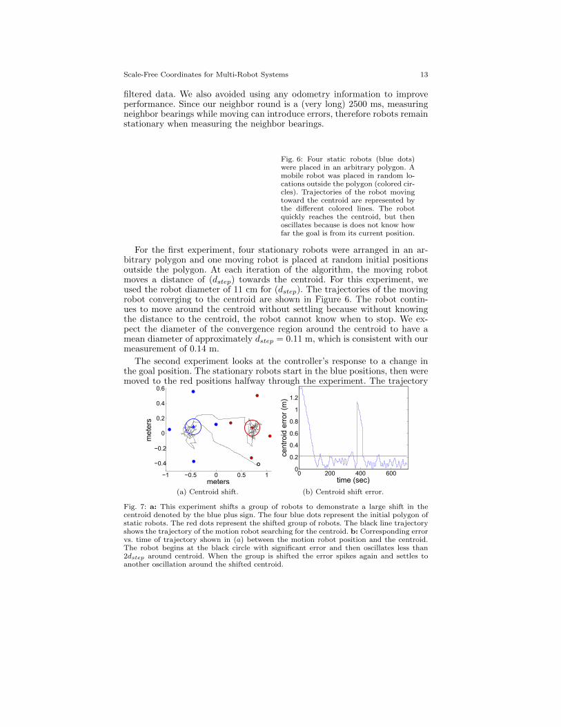
Fig. 6: Four static robots (blue dots)were placed in an arbitrary polygon. Amobile robot was placed in random lo-cations outside the polygon (colored cir-cles). Trajectories of the robot movingtoward the centroid are represented bythe different colored lines. The robotquickly reaches the centroid, but thenoscillates because is does not know howfar the goal is from its current position.

For the first experiment, four stationary robots were arranged in an ar-bitrary polygon and one moving robot is placed at random initial positionsoutside the polygon. At each iteration of the algorithm, the moving robotmoves a distance of (dstep) towards the centroid. For this experiment, weused the robot diameter of 11 cm for (dstep). The trajectories of the movingrobot converging to the centroid are shown in Figure 6. The robot contin-ues to move around the centroid without settling because without knowingthe distance to the centroid, the robot cannot know when to stop. We ex-pect the diameter of the convergence region around the centroid to have amean diameter of approximately dstep = 0.11 m, which is consistent with ourmeasurement of 0.14 m.

The second experiment looks at the controller’s response to a change inthe goal position. The stationary robots start in the blue positions, then weremoved to the red positions halfway through the experiment. The trajectory

60

−1 −0.5 0 0.5 1

−0.4

−0.2

0

0.2

0.4

0.6

meters

meters

(a) Centroid shift.

0 200 400 6000

0.2

0.4

0.6

0.8

1

1.2

cent

roid

err

or (

m)

time (sec)

(b) Centroid shift error.

Figure 6.5: a: This experiment moves a group of robots to demonstrate a large shift in the

centroid denoted by the blue plus sign. The four blue dots are the initial polygon

of static robots. The red dots represent the shifted group of robots. The black line

trajectory shows the trajectory of the motion robot searching for the centroid. The

red and blue circles represent the convergence of a fixed step size with a radius of

11cm. The robot is expected to oscillate within this circle. b: Corresponding error

vs. time of the trajectory shown in Sub-figure (a) between the motion robot position

and the centroid. The robot begins at the black circle with significant error and then

oscillates less than dstep radius around centroid. When the group is shifted the error

spikes again and settles to another oscillation around the new centroid.

6.3 Dynamic Evaluation: Tracking Motion

This experiment set out to track motion trajectory of the moving robot using scale-free

coordinates on the stationary robots. Analyzing scale-free coordinates between multiple

robots increases the volume of data to process. The experiment consisted of five stationary

robots in a connected graph configuration. A motion robot traversed this network with a

pre-defined straight line motion. The stationary robots produced an estimated position of

the motion robot with with scale-free coordinates and a α scaling factor. When combined

together at each time instance, this trajectory provides a reasonable estimate of the motion

(a) Centroid shift.

60

−1 −0.5 0 0.5 1

−0.4

−0.2

0

0.2

0.4

0.6

meters

meters

(a) Centroid shift.

0 200 400 6000

0.2

0.4

0.6

0.8

1

1.2

cent

roid

err

or (

m)

time (sec)

(b) Centroid shift error.

Figure 6.5: a: This experiment moves a group of robots to demonstrate a large shift in the

centroid denoted by the blue plus sign. The four blue dots are the initial polygon

of static robots. The red dots represent the shifted group of robots. The black line

trajectory shows the trajectory of the motion robot searching for the centroid. The

red and blue circles represent the convergence of a fixed step size with a radius of

11cm. The robot is expected to oscillate within this circle. b: Corresponding error

vs. time of the trajectory shown in Sub-figure (a) between the motion robot position

and the centroid. The robot begins at the black circle with significant error and then

oscillates less than dstep radius around centroid. When the group is shifted the error

spikes again and settles to another oscillation around the new centroid.

6.3 Dynamic Evaluation: Tracking Motion

This experiment set out to track motion trajectory of the moving robot using scale-free

coordinates on the stationary robots. Analyzing scale-free coordinates between multiple

robots increases the volume of data to process. The experiment consisted of five stationary

robots in a connected graph configuration. A motion robot traversed this network with a

pre-defined straight line motion. The stationary robots produced an estimated position of

the motion robot with with scale-free coordinates and a α scaling factor. When combined

together at each time instance, this trajectory provides a reasonable estimate of the motion

(b) Centroid shift error.

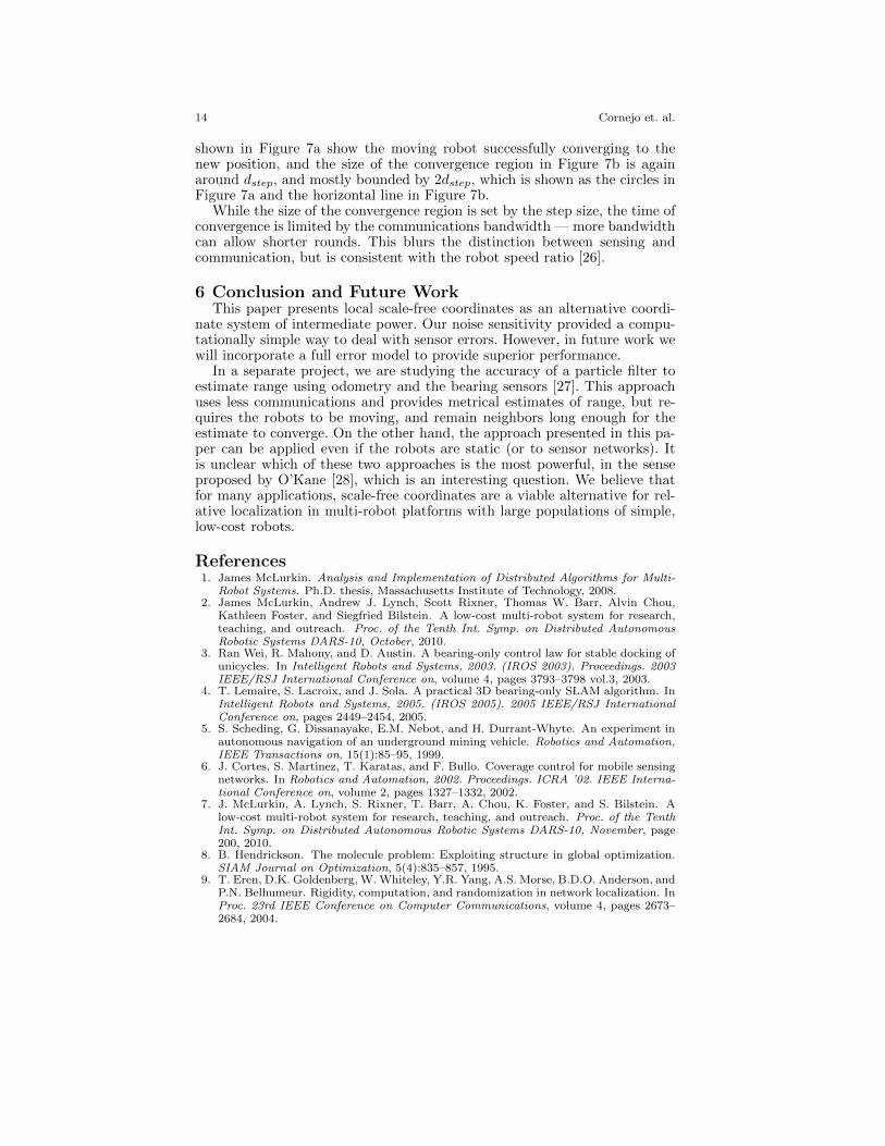
Fig. 7: a: This experiment shifts a group of robots to demonstrate a large shift in thecentroid denoted by the blue plus sign. The four blue dots represent the initial polygon ofstatic robots. The red dots represent the shifted group of robots. The black line trajectoryshows the trajectory of the motion robot searching for the centroid. b: Corresponding errorvs. time of trajectory shown in (a) between the motion robot position and the centroid.The robot begins at the black circle with significant error and then oscillates less than2dstep around centroid. When the group is shifted the error spikes again and settles toanother oscillation around the shifted centroid.

14 Cornejo et. al.

shown in Figure 7a show the moving robot successfully converging to thenew position, and the size of the convergence region in Figure 7b is againaround dstep, and mostly bounded by 2dstep, which is shown as the circles inFigure 7a and the horizontal line in Figure 7b.

While the size of the convergence region is set by the step size, the time ofconvergence is limited by the communications bandwidth — more bandwidthcan allow shorter rounds. This blurs the distinction between sensing andcommunication, but is consistent with the robot speed ratio [26].

6 Conclusion and Future WorkThis paper presents local scale-free coordinates as an alternative coordi-

nate system of intermediate power. Our noise sensitivity provided a compu-tationally simple way to deal with sensor errors. However, in future work wewill incorporate a full error model to provide superior performance.

In a separate project, we are studying the accuracy of a particle filter toestimate range using odometry and the bearing sensors [27]. This approachuses less communications and provides metrical estimates of range, but re-quires the robots to be moving, and remain neighbors long enough for theestimate to converge. On the other hand, the approach presented in this pa-per can be applied even if the robots are static (or to sensor networks). Itis unclear which of these two approaches is the most powerful, in the senseproposed by O’Kane [28], which is an interesting question. We believe thatfor many applications, scale-free coordinates are a viable alternative for rel-ative localization in multi-robot platforms with large populations of simple,low-cost robots.

References1. James McLurkin. Analysis and Implementation of Distributed Algorithms for Multi-

Robot Systems. Ph.D. thesis, Massachusetts Institute of Technology, 2008.2. James McLurkin, Andrew J. Lynch, Scott Rixner, Thomas W. Barr, Alvin Chou,

Kathleen Foster, and Siegfried Bilstein. A low-cost multi-robot system for research,teaching, and outreach. Proc. of the Tenth Int. Symp. on Distributed AutonomousRobotic Systems DARS-10, October, 2010.

3. Ran Wei, R. Mahony, and D. Austin. A bearing-only control law for stable docking ofunicycles. In Intelligent Robots and Systems, 2003. (IROS 2003). Proceedings. 2003IEEE/RSJ International Conference on, volume 4, pages 3793–3798 vol.3, 2003.

4. T. Lemaire, S. Lacroix, and J. Sola. A practical 3D bearing-only SLAM algorithm. InIntelligent Robots and Systems, 2005. (IROS 2005). 2005 IEEE/RSJ InternationalConference on, pages 2449–2454, 2005.

5. S. Scheding, G. Dissanayake, E.M. Nebot, and H. Durrant-Whyte. An experiment inautonomous navigation of an underground mining vehicle. Robotics and Automation,IEEE Transactions on, 15(1):85–95, 1999.

6. J. Cortes, S. Martinez, T. Karatas, and F. Bullo. Coverage control for mobile sensingnetworks. In Robotics and Automation, 2002. Proceedings. ICRA ’02. IEEE Interna-tional Conference on, volume 2, pages 1327–1332, 2002.

7. J. McLurkin, A. Lynch, S. Rixner, T. Barr, A. Chou, K. Foster, and S. Bilstein. Alow-cost multi-robot system for research, teaching, and outreach. Proc. of the TenthInt. Symp. on Distributed Autonomous Robotic Systems DARS-10, November, page200, 2010.

8. B. Hendrickson. The molecule problem: Exploiting structure in global optimization.SIAM Journal on Optimization, 5(4):835–857, 1995.

9. T. Eren, D.K. Goldenberg, W. Whiteley, Y.R. Yang, A.S. Morse, B.D.O. Anderson, andP.N. Belhumeur. Rigidity, computation, and randomization in network localization. InProc. 23rd IEEE Conference on Computer Communications, volume 4, pages 2673–2684, 2004.

Scale-Free Coordinates for Multi-Robot Systems 15

10. Kostas E. Bekris, A. A. Argyros, and L. E. Kavraki. Angle-based methods for mobilerobot navigation: Reaching the entire plane. In Proc. EEE International Conferenceon Robotics and Automation (ICRA), pages 2373–2378, 2004.

11. R. Nagpal, H. Shrobe, and J. Bachrach. Organizing a global coordinate system fromlocal information on an ad hoc sensor network. Proc. of Information Processing inSensor Networks (IPSN), 2003.

12. Pradeep Ranganathan, Ryan Morton, Andrew Richardson, Johannes Strom, RobertGoeddel, Mihai Bulic, and Edwin Olson. Coordinating a team of robots for urbanreconnaisance. In Proceedings of the Land Warfare Conference (LWC), November2010.

13. D. Moore, J. Leonard, D. Rus, and S. Teller. Robust distributed network localizationwith noisy range measurements. In In Proc. 2nd international conference on Embeddednetworked sensor systems, pages 50–61, 2004.

14. Nissanka B. Priyantha, Anit Chakraborty, and Hari Balakrishnan. The cricketlocation-support system. In Proceedings of the 6th annual international conferenceon Mobile computing and networking, pages 32–43, Boston, Massachusetts, UnitedStates, 2000. ACM.

15. Sooyong Lee, Nancy M. Amato, and James Fellers. Localization based on visibilitysectors using range sensors. In Proc. IEEE Int. Conf. Robot. Autom. (ICRA), pages3505–3511, 2000.

16. B. Sundaram, M. Palaniswami, S. Reddy, and M. Sinickas. Radar localization withmultiple unmanned aerial vehicles using support vector regression. In Intelligent Sens-ing and Information Processing, 2005. ICISIP 2005. Third International Conferenceon, pages 232 –237, 2005.

17. L. Montesano, J. Gaspar, J. Santos-Victor, and L. Montano. Cooperative localizationby fusing vision-based bearing measurements and motion. In Intelligent Robots andSystems, 2005. (IROS 2005). 2005 IEEE/RSJ International Conference on, pages2333 – 2338, August 2005.

18. S.G. Loizou and V. Kumar. Biologically inspired bearing-only navigation and tracking.In Decision and Control, 2007 46th IEEE Conference on, pages 1386 –1391, 2007.

19. Robert Ghrist, David Lipsky, Sameera Poduri, and Gaurav S. Sukhatme. Surroundingnodes in coordinate-free networks. In Workshop on the Algorithmic Foundations ofRobotics, 2006.

20. Davide Bil, Yann Disser, Mat Mihalk, Subhash Suri, Elias Vicari, and Peter Widmayer.Reconstructing visibility graphs with simple robots. In Structural Information andCommunication Complexity, pages 87–99, 2010.

21. W. Whiteley. Matroids from Discrete Geometry. AMS Contemporary Mathematics,197:171–312, 1996.

22. Jehoshua Bruck, Jie Gao, and Anxiao (Andrew) Jiang. Localization and routing insensor networks by local angle information. ACM Transactions on Sensor Networks,5(1):7:1–7:11, February 2009.

23. A. Cornejo, M. Khabbazian, and J. McLurkin. Theory of scale-free coor-dinates for multi-robot system with bearing-only sensors. Technical Report,http://mrsl.rice.edu/publications, 2011.

24. J. D. Horton. A Polynomial-Time algorithm to find the shortest cycle basis of a graph.SIAM Journal on Computing, 16(2):358, 1987.

25. Edwin Olson. Apriltag: A robust and flexible multi-purpose fiducial system. Technicalreport, University of Michigan APRIL Laboratory, May 2010.

26. J. McLurkin. Measuring the accuracy of distributed algorithms on Multi-Robot sys-tems with dynamic network topologies. 9th International Symposium on DistributedAutonomous Robotic Systems (DARS), 2008.

27. J. B. Rykowski. Pose Estimation With Low-Resolution Bearing-Only Sensors. M.S.thesis, Rice University, 2011.

28. J. M. O’Kane and S. M. LaValle. Comparing the power of robots. The InternationalJournal of Robotics Research, 27(1):5, 2008.