Embed Size (px)
Citation preview

Scalar Field Visualization
Some slices used by Prof. Mike Bailey
Scalar Fields
• The approximation of certain scalar function
in space f(x,y,z).
• Most of time, they come in as some scalar
values defined on some sample points.
• Visualization primitives: colors, transparency,
iso-contours (2D), iso-surfaces (3D), 3D
textures.

In OpenGL, the mapping of 1D texture
In Visualization, we Use the Concept of a Transfer
Function to set Color as a Function of Scalar Value
Scalar values ->[0,1] -> Colors ��� � 240. 240. ��
��� ��

2D Interpolated Color Plots
• Here’s the situation: we have a 2D grid of data points. At each
node, we have an X, Y, Z, and a scalar value S. We know Smin,
Smax, and the Transfer Function.
Even though this is a 2D technique, we keep around
the X, Y, and Z coordinates so that the grid doesn’t
have to lie in any particular plane.

2D Interpolated Color Plots
• We deal with one square of the mesh at a time
We let OpenGL deal with the color interpolation
float hsv[3], rgb[3]
!"[0] � 240. 240. ��
��� ��
HsvRgb (hsv, rgb)

2D Interpolated Color Plots
• We let OpenGL deal with the color interpolation
// compute color at V0
glColor3f (r0, g0, b0);
glVertex3f (x0, y0, z0);
// compute color at V1
glColor3f (r1, g1, b1);
glVertex3f (x1, y1, z1);
// compute color at V3
glColor3f (r3, g3, b3);
glVertex3f (x3, y3, z3);
// compute color at V2
glColor3f (r2, g2, b2);
glVertex3f (x2, y2, z2);

A Gallery of Color Scales

Iso-Contouring and Iso-Surfacing
for Scalar Field Visualization

2D Contour Lines
• Here’s the situation: we have a 2D grid of data points. At each
node, we have an X, Y, Z, and a scalar value S. We know the
Transfer Function. We also have a particular scalar value, S*,
at which we want to draw the contour line(s).

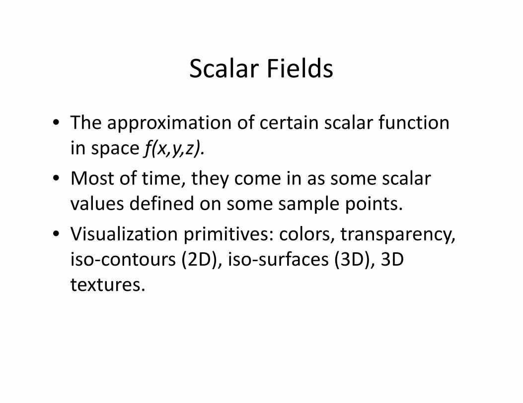
2D Contour Lines: Marching Squares
• Rather than deal with the entire grid, we deal with one square
at a time, marching through them all. For this reason, this
method is called the Marching Squares.
Marching Squares
• What’s really going to happen is that we are not creating contours by connecting
points into a complete curve. We are creating contours by drawing a collection of
2-point line segments, safe in the knowledge that those line segments will align
across square boundaries.
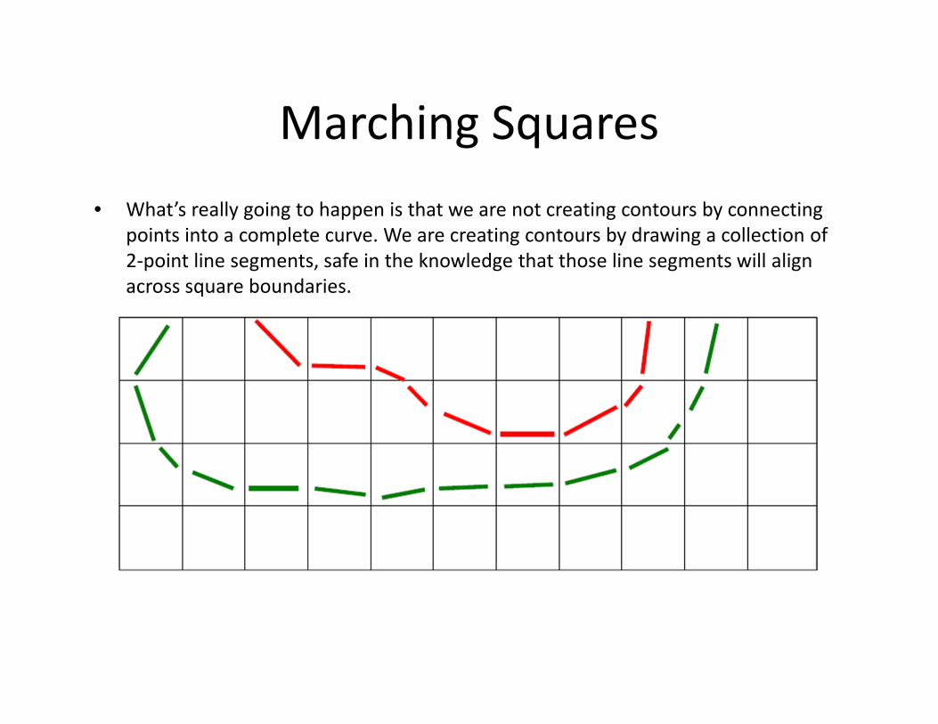
Marching Squares
Does S* cross any edges of this square?
Linearly interpolating the scalar value from node 0 to node 1 gives:
� 1 $ % & $' � % & $('%) where 0. * $ * 1.
Setting this interpolated S equal to S* and solving for t gives:
$∗ �∗ %
' %
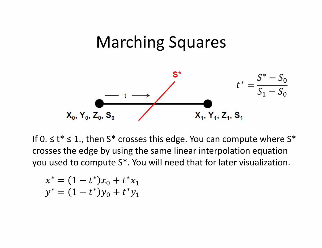
Marching Squares
If 0. ≤ t* ≤ 1., then S* crosses this edge. You can compute where S*
crosses the edge by using the same linear interpolation equation
you used to compute S*. You will need that for later visualization.
$∗ �∗ %
' %
,∗ � 1 $∗ ,% & $∗,'
-∗ � 1 $∗ -% & $∗-'

Marching Squares
• Do this for all 4 edges – when you are done, there are 5
possible ways this could have turned out
– # of intersections = 0
– # of intersections = 2
– # of intersections = 1
– # of intersections = 3

Marching Squares
• Do this for all 4 edges – when you are done, there are 5
possible ways this could have turned out
– # of intersections = 0 Do nothing
– # of intersections = 2 Draw a line connecting them
– # of intersections = 1
– # of intersections = 3
Error: this means that the contour got
into the square and never got out
Error: this means that the contour got
into the square and never got out
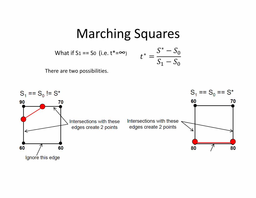
Marching Squares
What if S1 == S0 (i.e. t*=∞)
There are two possibilities.
$∗ �∗ %
' %

Marching Squares
What if there are four intersections
This means that going around the square, the
nodes are >S*, <S*, >S*, and <S* in that order.
This gives us a saddle function, shown here in
cyan.
If we think of the scalar values as terrain
heights, then we can think of S* as the height of
water that is flooding the terrain, as shown here
in magenta
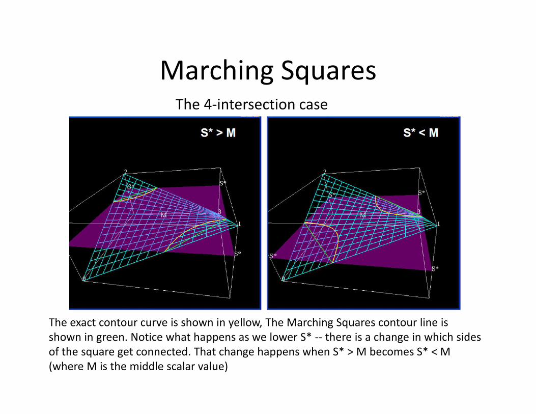
Marching SquaresThe 4-intersection case
The exact contour curve is shown in yellow, The Marching Squares contour line is
shown in green. Notice what happens as we lower S* -- there is a change in which sides
of the square get connected. That change happens when S* > M becomes S* < M
(where M is the middle scalar value)

Marching SquaresThe 4-intersection case: Compute the middle scalar value
Let’s linearly interpolate scalar values along the 0-1 edge, and along the 2-3 edge:
%' � 1 $ % & $'
./ � 1 $ . & $/
Now linearly interpolate these two linearly-interpolated scalar values:
($, �) � 1 � %' & �./
Expand this we get
$, � � 1 $ 1 � % & $(1 �)' & 1 $ �. & $�/
This is the bilinear interpolation equation.
0 1
2 3
t
u
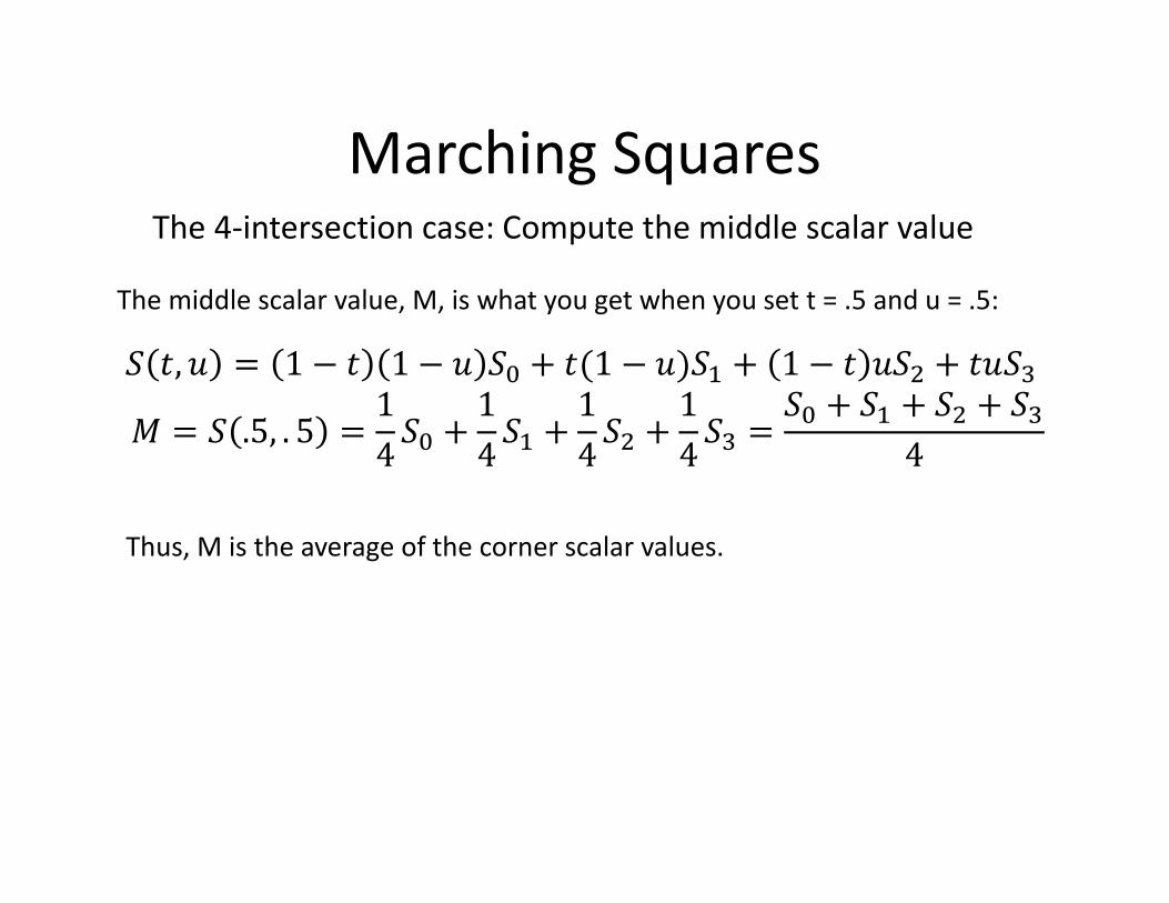
Marching SquaresThe 4-intersection case: Compute the middle scalar value
The middle scalar value, M, is what you get when you set t = .5 and u = .5:
$, � � 1 $ 1 � % & $(1 �)' & 1 $ �. & $�/
0 � .5, . 5 �1
4% &
1
4' &
1
4. &
1
4/ �
% & ' & . & /
4
Thus, M is the average of the corner scalar values.
Marching SquaresThe 4-intersection case: Compute the middle scalar value
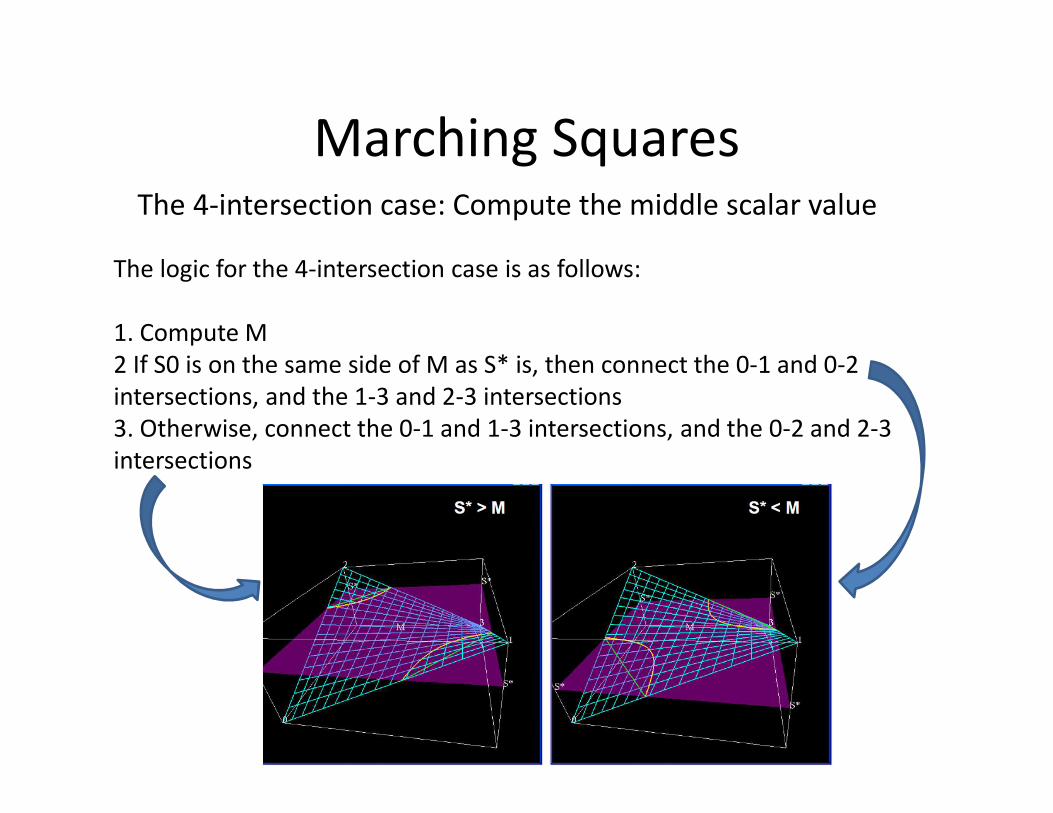
The logic for the 4-intersection case is as follows:
1. Compute M
2 If S0 is on the same side of M as S* is, then connect the 0-1 and 0-2
intersections, and the 1-3 and 2-3 intersections
3. Otherwise, connect the 0-1 and 1-3 intersections, and the 0-2 and 2-3
intersections

Artifacts?
What if the distribution of scalar values along the square edges isn’t linear?
What if you have a contour that really looks like this?
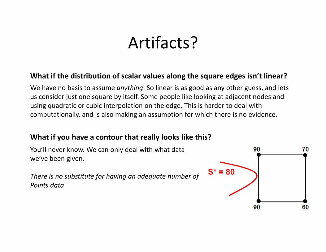
Artifacts?
What if the distribution of scalar values along the square edges isn’t linear?
What if you have a contour that really looks like this?
We have no basis to assume anything. So linear is as good as any other guess, and lets
us consider just one square by itself. Some people like looking at adjacent nodes and
using quadratic or cubic interpolation on the edge. This is harder to deal with
computationally, and is also making an assumption for which there is no evidence.
You’ll never know. We can only deal with what data
we’ve been given.
There is no substitute for having an adequate number of
Points data
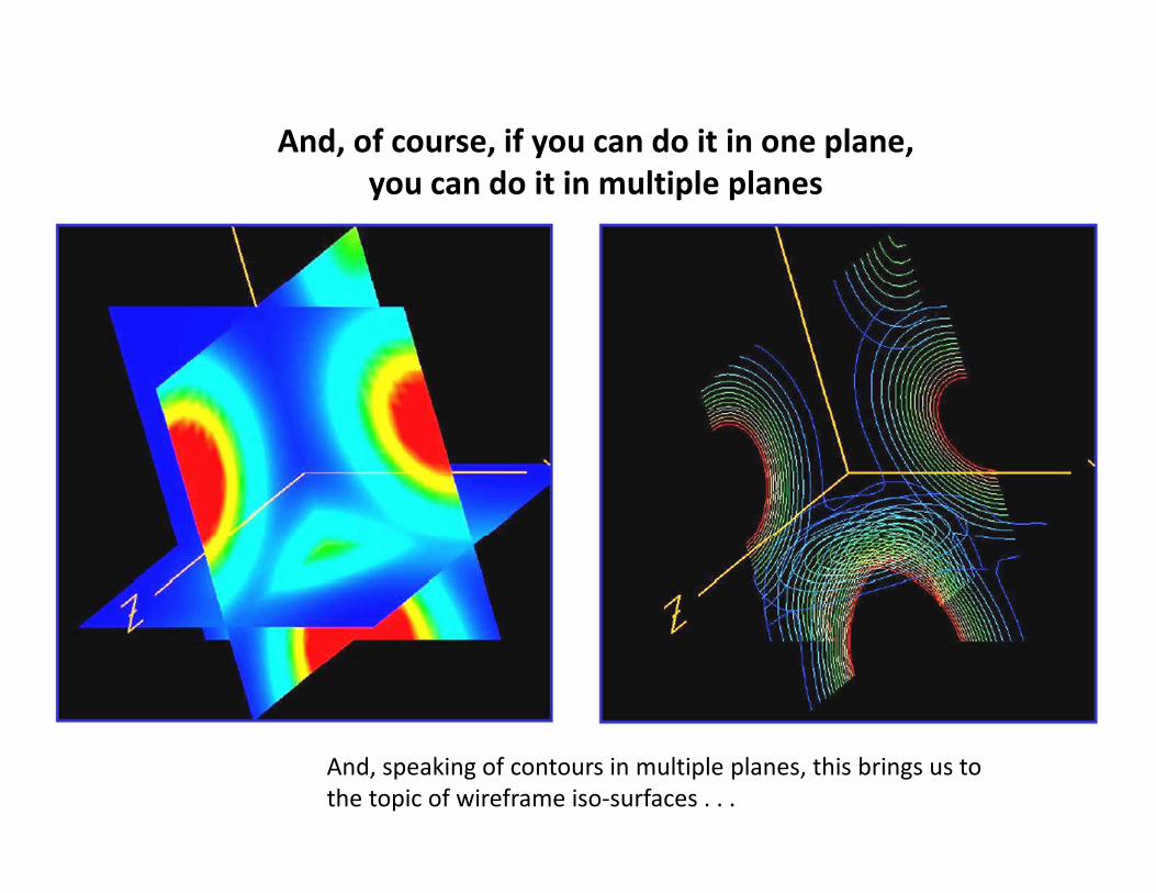
And, of course, if you can do it in one plane,
you can do it in multiple planes
And, speaking of contours in multiple planes, this brings us to
the topic of wireframe iso-surfaces . . .

Iso-surfacing
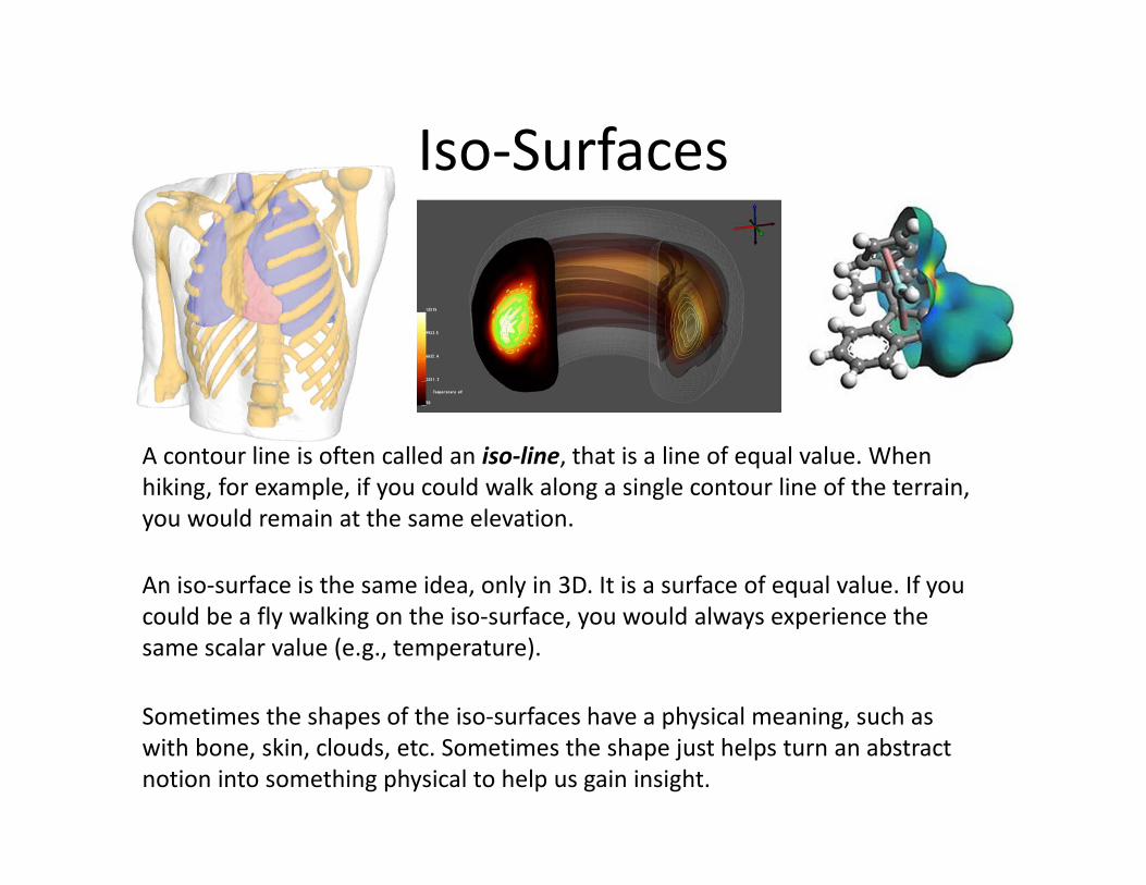
Iso-Surfaces
A contour line is often called an iso-line, that is a line of equal value. When
hiking, for example, if you could walk along a single contour line of the terrain,
you would remain at the same elevation.
An iso-surface is the same idea, only in 3D. It is a surface of equal value. If you
could be a fly walking on the iso-surface, you would always experience the
same scalar value (e.g., temperature).
Sometimes the shapes of the iso-surfaces have a physical meaning, such as
with bone, skin, clouds, etc. Sometimes the shape just helps turn an abstract
notion into something physical to help us gain insight.
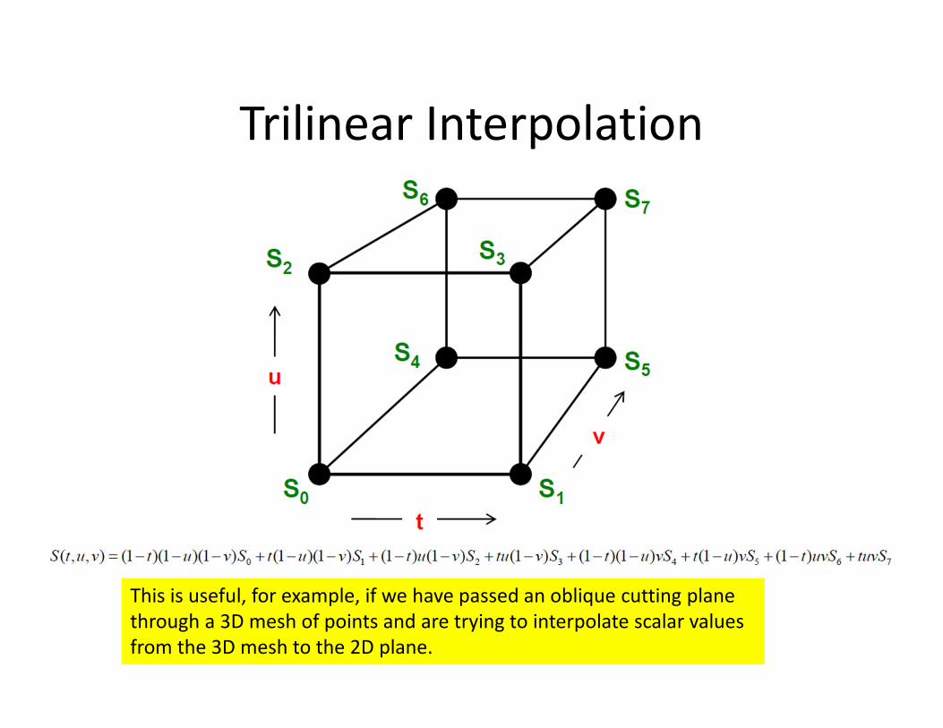
Trilinear Interpolation
This is useful, for example, if we have passed an oblique cutting plane
through a 3D mesh of points and are trying to interpolate scalar values
from the 3D mesh to the 2D plane.
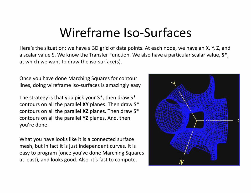
Wireframe Iso-SurfacesHere’s the situation: we have a 3D grid of data points. At each node, we have an X, Y, Z, and
a scalar value S. We know the Transfer Function. We also have a particular scalar value, S*,
at which we want to draw the iso-surface(s).
Once you have done Marching Squares for contour
lines, doing wireframe iso-surfaces is amazingly easy.
The strategy is that you pick your S*, then draw S*
contours on all the parallel XY planes. Then draw S*
contours on all the parallel XZ planes. Then draw S*
contours on all the parallel YZ planes. And, then
you’re done.
What you have looks like it is a connected surface
mesh, but in fact it is just independent curves. It is
easy to program (once you’ve done Marching Squares
at least), and looks good. Also, it’s fast to compute.
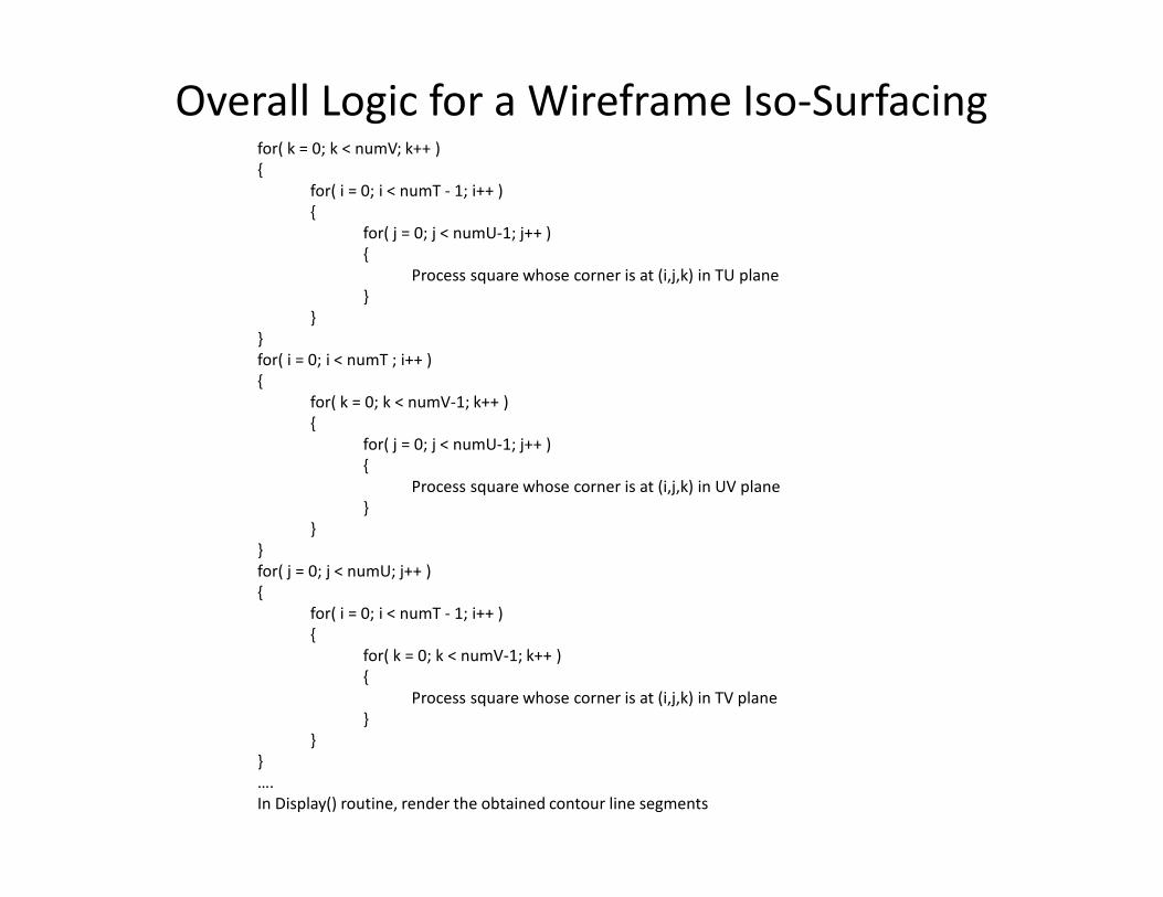
Overall Logic for a Wireframe Iso-Surfacingfor( k = 0; k < numV; k++ )
{
for( i = 0; i < numT - 1; i++ )
{
for( j = 0; j < numU-1; j++ )
{
Process square whose corner is at (i,j,k) in TU plane
}
}
}
for( i = 0; i < numT ; i++ )
{
for( k = 0; k < numV-1; k++ )
{
for( j = 0; j < numU-1; j++ )
{
Process square whose corner is at (i,j,k) in UV plane
}
}
}
for( j = 0; j < numU; j++ )
{
for( i = 0; i < numT - 1; i++ )
{
for( k = 0; k < numV-1; k++ )
{
Process square whose corner is at (i,j,k) in TV plane
}
}
}
….
In Display() routine, render the obtained contour line segments

Iso-surface Construction:
Marching Cubes
Iso-surface Construction:
Marching Cubes
• For simplicity, we shall work with zero level
(s*=0) iso-surface, and denote
positive vertices as
There are EIGHT vertices, each can be positive
or negative - so there are 28 = 256 different cases!
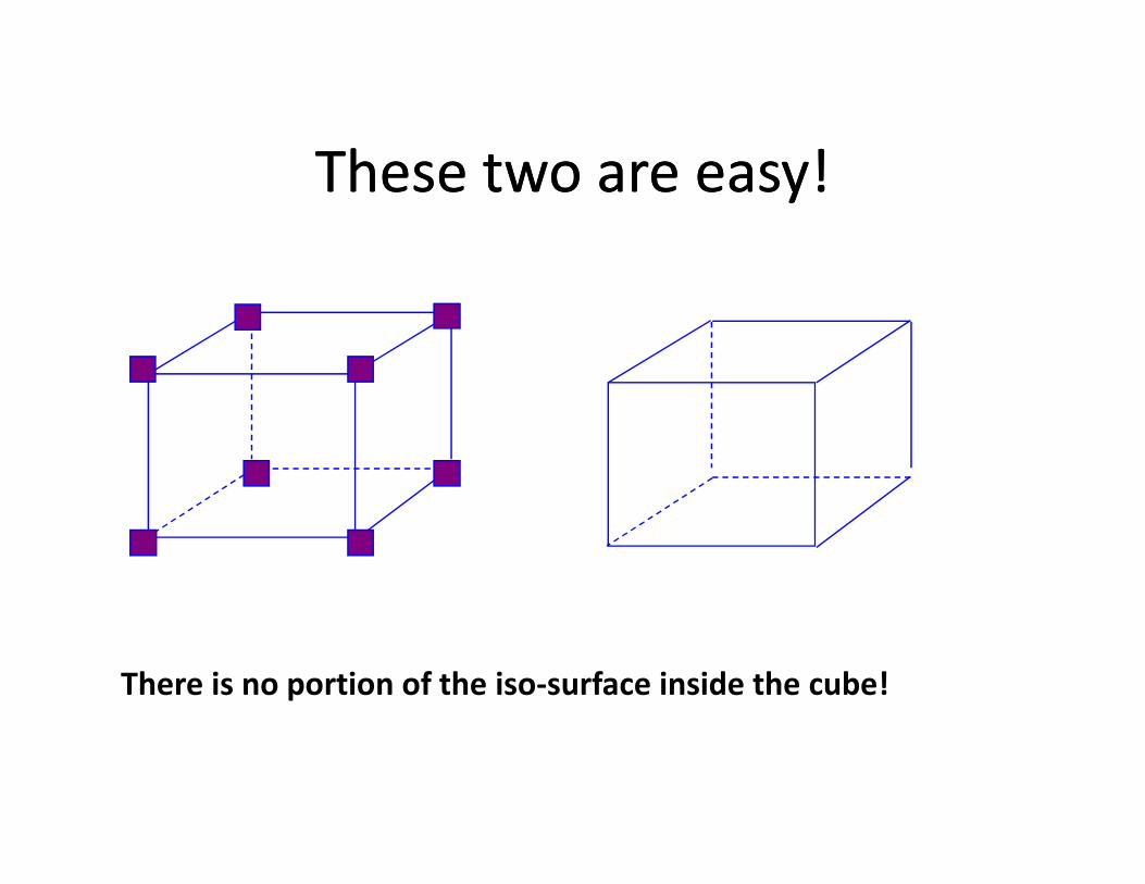
These two are easy!These two are easy!
There is no portion of the iso-surface inside the cube!
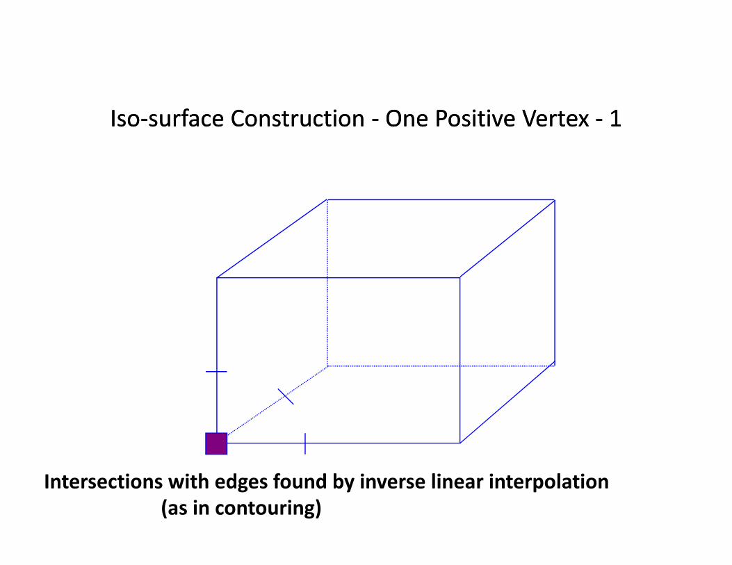
Iso-surface Construction - One Positive Vertex - 1Iso-surface Construction - One Positive Vertex - 1
Intersections with edges found by inverse linear interpolation
(as in contouring)
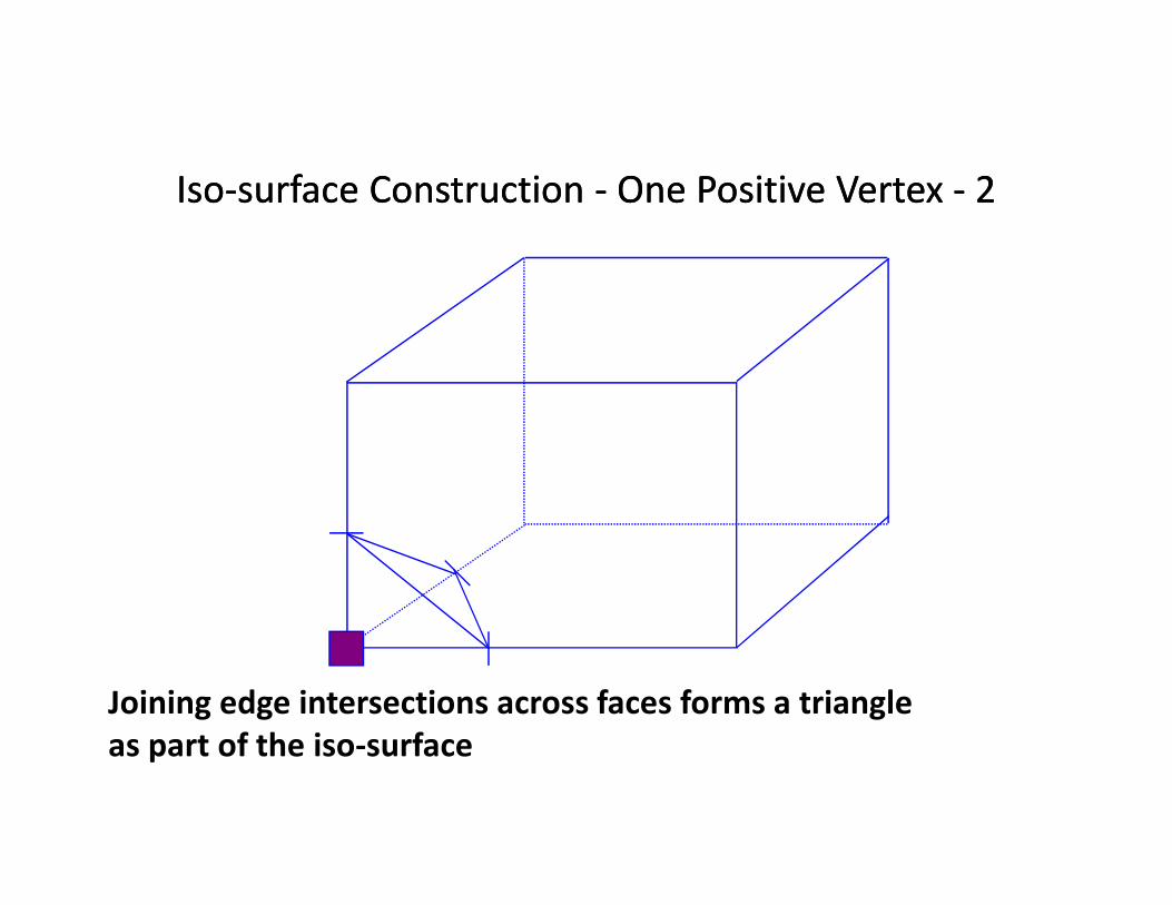
Iso-surface Construction - One Positive Vertex - 2Iso-surface Construction - One Positive Vertex - 2
Joining edge intersections across faces forms a triangle
as part of the iso-surface
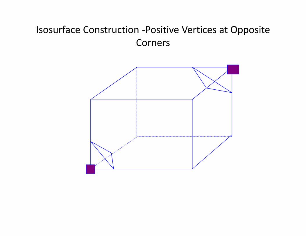
Isosurface Construction -Positive Vertices at Opposite
Corners

Iso-surface Construction:
Marching Cubes
Iso-surface Construction:
Marching Cubes
• One can work through all 256 cases in this way -although it quickly becomes apparent that many cases are similar.
• For example:
– 2 cases where all are positive, or all negative, give no isosurface
– 16 cases where one vertex has opposite sign from all the rest
• In fact, there are only 15 topologically distinct configurations
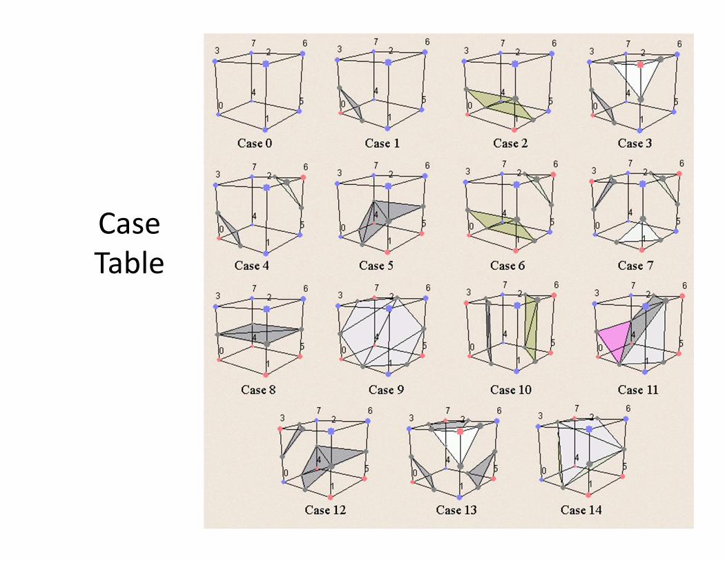
Case
Table

8 Above
0 Below
1 case

7 Above
1 Below
1 case

6 Above
2 Below
3 cases

5 Above
3 Below
3 cases

4 Above
4 Below
7 cases

4 Above
4 Below
7 cases
4 edge-connected
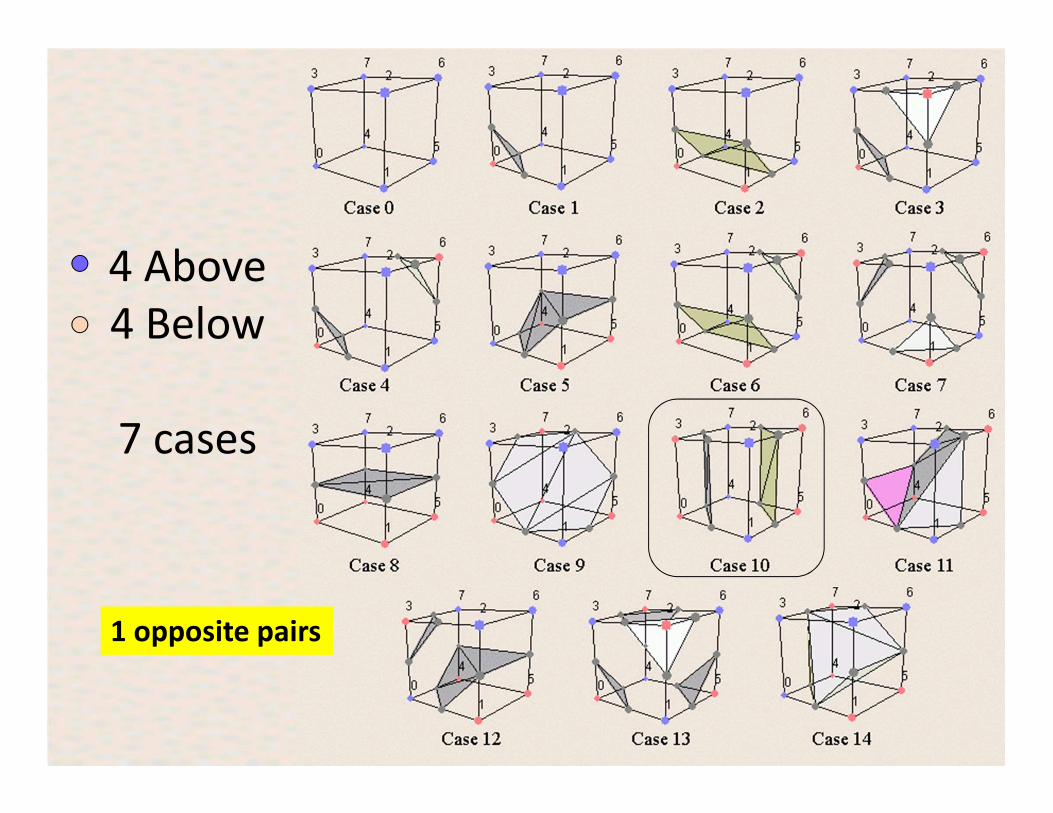
4 Above
4 Below
7 cases
1 opposite pairs

4 Above
4 Below
7 cases
1 vertex opposite
to triplet
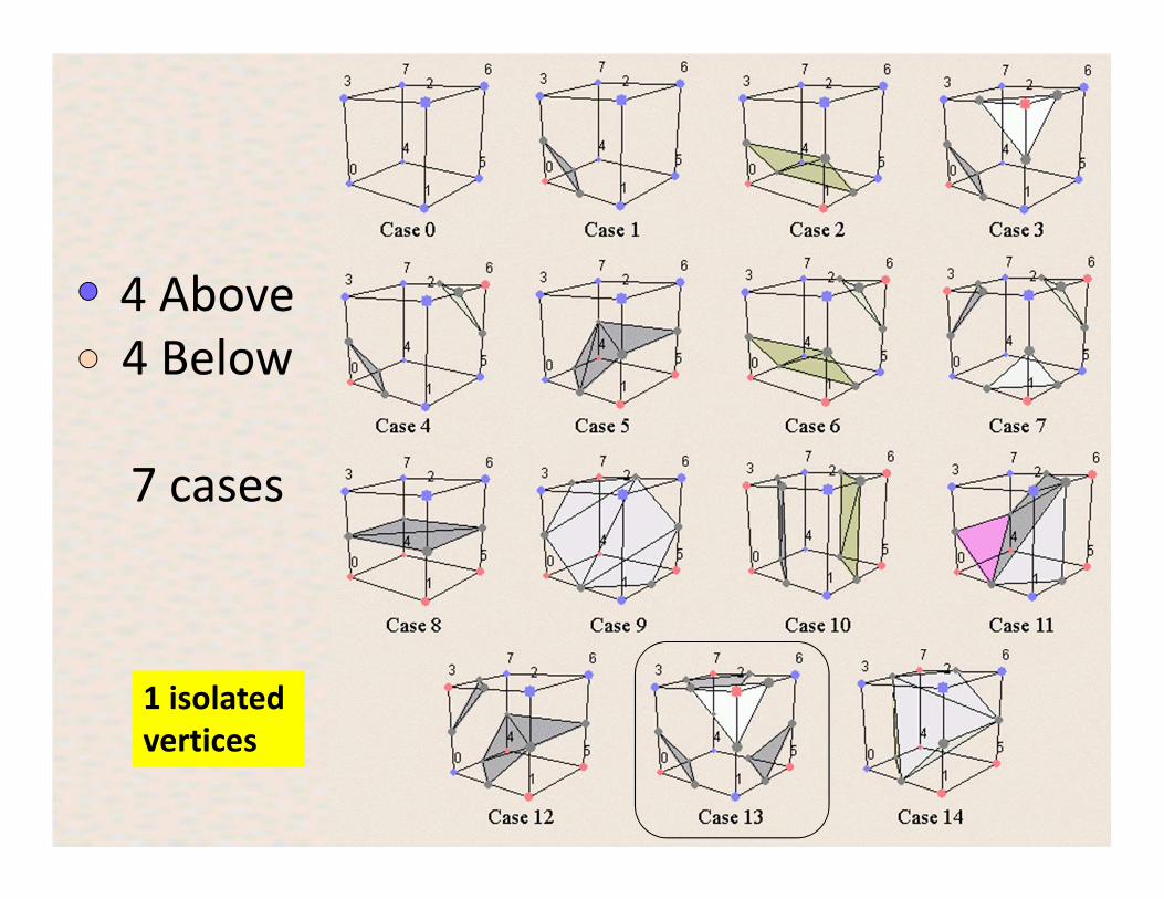
4 Above
4 Below
7 cases
1 isolated
vertices
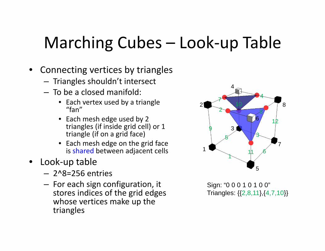
Marching Cubes – Look-up Table
• Connecting vertices by triangles – Triangles shouldn’t intersect
– To be a closed manifold:• Each vertex used by a triangle
“fan”
• Each mesh edge used by 2 triangles (if inside grid cell) or 1 triangle (if on a grid face)
• Each mesh edge on the grid face is shared between adjacent cells
• Look-up table– 2^8=256 entries
– For each sign configuration, it stores indices of the grid edges whose vertices make up the triangles
1
2
3
4
5
6
7
8
1
2
3
4
5
6
7
8
9
10
11
12
Sign: “0 0 0 1 0 1 0 0”Triangles: {{2,8,11},{4,7,10}}

Further Readings
• Marching Cubes:• “Marching cubes: A high resolution 3D surface
construction algorithm”, by Lorensen and Cline (1987)
– >6000 citations on Google Scholar
• “A survey of the marching cubes algorithm”, by Newman and Yi (2006)
• Dual Contouring:• “Dual contouring of hermite data”, by Ju et al. (2002)
– >300 citations on Google Scholar
• “Manifold dual contouring”, by Schaefer et al. (2007)

Polygonal Iso-Surfaces (Optional)
Marching Cubes is difficult, and so we will look at another approach.

Polygonal Iso-Surfaces: Data Structure

bool FoundEdgeIntersection[12]
One entry for each of the 12 edges.
false means S* did not intersect this edge
true means S* did intersect this edge
Node EdgeIntersection[12]
If an intersection did occur on edge #i, Node[i] will contain the
interpolated x, y, z, nx, ny, and nz.
bool FoundEdgeConnection[12][12]
A true in entry [i][j] or [j][i] means that Marching Squares has decided there
needs to be a line drawn from Cube Edge #i to Cube Edge #j
Both entry [i][j] and [j][i] are filled so that it won’t matter which order you
search in later.
Polygonal Iso-Surfaces: Data Structure

Polygonal Iso-Surfaces: Algorithm
Strategy in ProcessCube():
1. Use ProcessCubeEdge() 12 times to find which cube edges have S*
intersections.
2. Return if no intersections were found anywhere.
3. Call ProcessCubeQuad() 6 times to decide which cube edges will need to
be connected. This is Marching Squares like we did it before, but it doesn’t
need to re-compute intersections on the cube edges in common.
ProcessCubeEdge() already did that. This leaves us with the
FoundEdgeConnection[][] array filled.
4. Call DrawCubeTriangles() to create triangles from the connected edges.

Polygonal Iso-Surfaces: Algorithm
Strategy in DrawCubeTriangles():
1. Look through the FoundEdgeConnection[][] array for a Cube Edge #A
and a Cube Edge #B that have a connection between them.
2. If can’t find one, then you are done with this cube.
3. Now look through the FoundEdgeConnection[][] array for a Cube Edge
#C that is connected to Cube Edge #B. If you can’t find one, something is
wrong.
4. Draw a triangle using the EdgeIntersection[] nodes from Cube Edges
#A, #B, and #C. Be sure to use glNormal3f() in addition to glVertex3f().
5. Turn to false the FoundEdgeConnection[][]entries from Cube Edge #A
to Cube Edge #B.
6. Turn to false the FoundEdgeConnection[][]entries from Cube Edge #B
to Cube Edge #C.
7. Toggle the FoundEdgeConnection[][]entries from Cube Edge #C to
Cube Edge #A. If this connection was there before, we don’t need it
anymore. If it was not there before, then we just invented it and we will
need it again.

Polygonal Iso-Surfaces: Why Does this work?
Take this case as an example. The intersection points A, B, C,
and D were found and the lines AB, BC, CD, and DA were found
because Marching Squares will have been performed on each
of the cube’s 6 faces
At this point, we could just draw the quadrilateral ABCD, but
this will likely go wrong because it is surely non-planar. So,
starting at A, we break out a triangle from the edges AB and BC
(which exist) and the edge CA (which doesn’t exist, but we
need it anyway to complete the triangle).
When we toggle the FoundEdgeConnection[][] entries for AB
and BC, they turn from true to false. When we toggle the
FoundEdgeConnection[][] for CA, it turns from false to true
This leaves FoundEdgeConnection[][] for CA, CD, and AD all
set to true, which will cause the algorithm to find them and
connect them into a triangle next.
Note that this algorithm will eventually find and properly
connect the little triangle in the upper-right corner, even though
it has no connection with A-B-C-D.
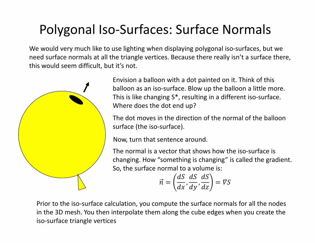
Polygonal Iso-Surfaces: Surface Normals
We would very much like to use lighting when displaying polygonal iso-surfaces, but we
need surface normals at all the triangle vertices. Because there really isn’t a surface there,
this would seem difficult, but it’s not.
Envision a balloon with a dot painted on it. Think of this
balloon as an iso-surface. Blow up the balloon a little more.
This is like changing S*, resulting in a different iso-surface.
Where does the dot end up?
The dot moves in the direction of the normal of the balloon
surface (the iso-surface).
Now, turn that sentence around.
The normal is a vector that shows how the iso-surface is
changing. How “something is changing” is called the gradient.
So, the surface normal to a volume is:
Prior to the iso-surface calculation, you compute the surface normals for all the nodes
in the 3D mesh. You then interpolate them along the cube edges when you create the
iso-surface triangle vertices
2 �3
3,,3
3-,3
34� 5


![[inria-00600161, v1] Visualization of uncertain scalar ... › files › 2011ACTI2650.pdf · Visualization of uncertain scalar data elds using color scales and perceptua lly adapted](https://img.pdfslide.us/doc/110x75/5f0bd40f7e708231d43269c8/inria-00600161-v1-visualization-of-uncertain-scalar-a-files-a-visualization.jpg)