Embed Size (px)
Citation preview

Scalar conservation laws with moving density constraintsarising in traffic flow modeling
Maria Laura Delle Monache
Email: maria-laura.delle [email protected].
Joint work with Paola Goatin
14th International Conference on Hyperbolic Problems:Theory, Numerics, ApplicationsUniversita di Padova
28, June 2012

Outline
Outline
1 Introduction
2 The Riemann problem with moving density constraint
3 The Cauchy problem: Existence of solutions
4 Conclusions
Maria Laura Delle Monache (INRIA) Scalar conservation laws with moving constraints 28, June 2012 2 / 24

Introduction
Outline
1 IntroductionMathematical ModelExisting Models
2 The Riemann problem with moving density constraintRiemann ProblemRiemann Solver
3 The Cauchy problem: Existence of solutionsCauchy ProblemWave-Front Tracking MethodBounds on the total variationConvergence of approximate solutionsExistence of weak solution
4 Conclusions
Maria Laura Delle Monache (INRIA) Scalar conservation laws with moving constraints 28, June 2012 3 / 24
Introduction Mathematical Model
Mathematical Model I
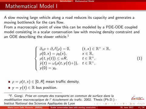
A slow moving large vehicle along a road reduces its capacity and generates amoving bottleneck for the cars flow.From a macroscopic point of view this can be modeled by a PDE-ODE coupledmodel consisting in a scalar conservation law with moving density constraint andan ODE describing the slower vehicle.1
∂tρ+ ∂x f (ρ) = 0, (t, x) ∈ R+ × R,ρ(0, x) = ρ0(x), x ∈ R,ρ(t, y(t)) ≤ αR, t ∈ R+,y(t) = ω(ρ(t, y(t)+)), t ∈ R+,y(0) = y0.
(1)
ρ = ρ(t, x) ∈ [0,R] mean traffic density.
y = y(t) ∈ R bus position.
1F. Giorgi. Prise en compte des transports en commun de surface dans lamodelisation macroscopique de l’ ecoulement du trafic. 2002. Thesis (Ph.D.) -Institut National des Sciences Appliquees de Lyon
Maria Laura Delle Monache (INRIA) Scalar conservation laws with moving constraints 28, June 2012 4 / 24
Introduction Mathematical Model
Mathematical Model II
ρα
f (ρ)
ρ
Vb
ρα ρ∗
ω(ρ)
Vb
v(ρ)
ρ∗ ρ
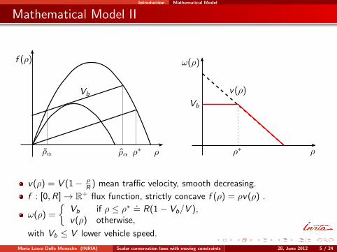
v(ρ) = V (1− ρR ) mean traffic velocity, smooth decreasing.
f : [0,R]→ R+ flux function, strictly concave f (ρ) = ρv(ρ) .
ω(ρ) =
Vb if ρ ≤ ρ∗ .= R(1− Vb/V ),v(ρ) otherwise,
with Vb ≤ V lower vehicle speed.
Maria Laura Delle Monache (INRIA) Scalar conservation laws with moving constraints 28, June 2012 5 / 24
Introduction Mathematical Model
Mathematical Model III
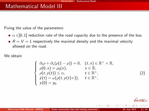
Fixing the value of the parameters:
α ∈]0, 1[ reduction rate of the road capacity due to the presence of the bus.
R = V = 1 respectively the maximal density and the maximal velocityallowed on the road.
We obtain ∂tρ+ ∂x (ρ(1− ρ)) = 0, (t, x) ∈ R+ × R,ρ(0, x) = ρ0(x), x ∈ R,ρ(t, y(t)) ≤ α, t ∈ R+,y(t) = ω(ρ(t, y(t)+)), t ∈ R+,y(0) = y0.
(2)
Maria Laura Delle Monache (INRIA) Scalar conservation laws with moving constraints 28, June 2012 6 / 24
Introduction Existing Models
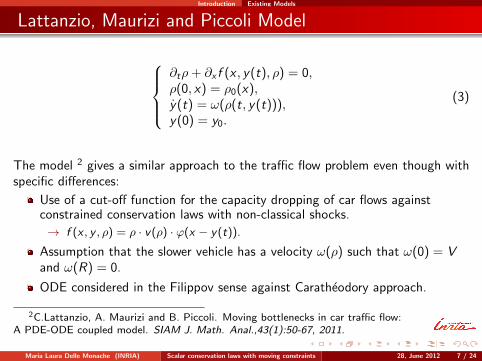
Lattanzio, Maurizi and Piccoli Model
∂tρ+ ∂x f (x , y(t), ρ) = 0,ρ(0, x) = ρ0(x),y(t) = ω(ρ(t, y(t))),y(0) = y0.
(3)
The model 2 gives a similar approach to the traffic flow problem even though withspecific differences:
Use of a cut-off function for the capacity dropping of car flows againstconstrained conservation laws with non-classical shocks.
→ f (x , y , ρ) = ρ · v(ρ) · ϕ(x − y(t)).
Assumption that the slower vehicle has a velocity ω(ρ) such that ω(0) = Vand ω(R) = 0.
ODE considered in the Filippov sense against Caratheodory approach.
2C.Lattanzio, A. Maurizi and B. Piccoli. Moving bottlenecks in car traffic flow:A PDE-ODE coupled model. SIAM J. Math. Anal.,43(1):50-67, 2011.
Maria Laura Delle Monache (INRIA) Scalar conservation laws with moving constraints 28, June 2012 7 / 24
Introduction Existing Models
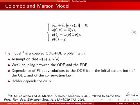
Colombo and Marson Model
∂tρ+ ∂x [ρ · v(ρ)] = 0,ρ(0, x) = ρ(x),p(t) = ω(ρ(t, p)),p(0) = p.
(4)
The model 3 is a coupled ODE-PDE problem with:
Assumption that ω(ρ) ≥ v(ρ) .
Weak coupling between the ODE and the PDE.
Dependence of Filippov solutions to the ODE from the initial datum both ofthe ODE and of the conservation law.
Holder dependence on p.
3R. M. Colombo and A. Marson. A Holder continuous ODE related to traffic flow.Proc. Roy. Soc. Edinburgh Sect. A, 133(4):759-772, 2003.
Maria Laura Delle Monache (INRIA) Scalar conservation laws with moving constraints 28, June 2012 8 / 24

The Riemann problem with moving density constraint
Outline
1 IntroductionMathematical ModelExisting Models
2 The Riemann problem with moving density constraintRiemann ProblemRiemann Solver
3 The Cauchy problem: Existence of solutionsCauchy ProblemWave-Front Tracking MethodBounds on the total variationConvergence of approximate solutionsExistence of weak solution
4 Conclusions
Maria Laura Delle Monache (INRIA) Scalar conservation laws with moving constraints 28, June 2012 9 / 24
The Riemann problem with moving density constraint Riemann Problem
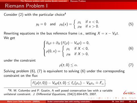
Riemann Problem I
Consider (2) with the particular choice4
y0 = 0 and ρ0(x) =
ρL if x < 0,ρR if x > 0.
(5)
Rewriting equations in the bus reference frame i.e., setting X = x − Vbt.We get
∂tρ+ ∂X (f (ρ)− Vbρ) = 0,
ρ(0, x) =
ρL if X < 0,
ρR if X > 0,
(6)
under the constraintρ(t, 0) ≤ α. (7)
Solving problem (6), (7) is equivalent to solving (6) under the correspondingconstraint on the flux
f (ρ(t, 0))− Vbρ(t, 0) ≤ fα(ρα)− Vbρα.
= Fα .
4R. M. Colombo and P. Goatin, A well posed conservation law with a variableunilateral constraint. J. Differential Equations, 234(2):654-675, 2007.
Maria Laura Delle Monache (INRIA) Scalar conservation laws with moving constraints 28, June 2012 10 / 24
The Riemann problem with moving density constraint Riemann Problem
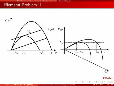
Riemann Problem II
ρα α
f (ρ)
ρ
Vb
ραρα 1
f (ρ)− Vbρ
Fα
ρα ρ
Vbρ
ραρα
Maria Laura Delle Monache (INRIA) Scalar conservation laws with moving constraints 28, June 2012 11 / 24
The Riemann problem with moving density constraint Riemann Solver
Riemann Solver
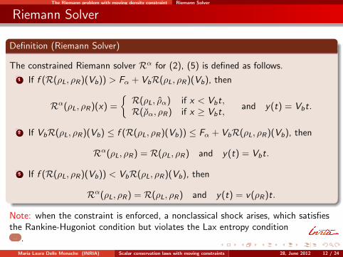
Definition (Riemann Solver)
The constrained Riemann solver Rα for (2), (5) is defined as follows.
1 If f (R(ρL, ρR )(Vb)) > Fα + VbR(ρL, ρR )(Vb), then
Rα(ρL, ρR )(x) =
R(ρL, ρα) if x < Vbt,R(ρα, ρR ) if x ≥ Vbt,
and y(t) = Vbt.
2 If VbR(ρL, ρR )(Vb) ≤ f (R(ρL, ρR )(Vb)) ≤ Fα + VbR(ρL, ρR )(Vb), then
Rα(ρL, ρR ) = R(ρL, ρR ) and y(t) = Vbt.
3 If f (R(ρL, ρR )(Vb)) < VbR(ρL, ρR )(Vb), then
Rα(ρL, ρR ) = R(ρL, ρR ) and y(t) = v(ρR )t.
Note: when the constraint is enforced, a nonclassical shock arises, which satisfiesthe Rankine-Hugoniot condition but violates the Lax entropy condition
... .
Maria Laura Delle Monache (INRIA) Scalar conservation laws with moving constraints 28, June 2012 12 / 24
The Riemann problem with moving density constraint Riemann Solver
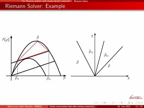
Riemann Solver: Example
f (ρ)
ρ
ρ
ρα ρα
ρρ
ραρα
x
t
Maria Laura Delle Monache (INRIA) Scalar conservation laws with moving constraints 28, June 2012 13 / 24

The Cauchy problem: Existence of solutions
Outline
1 IntroductionMathematical ModelExisting Models
2 The Riemann problem with moving density constraintRiemann ProblemRiemann Solver
3 The Cauchy problem: Existence of solutionsCauchy ProblemWave-Front Tracking MethodBounds on the total variationConvergence of approximate solutionsExistence of weak solution
4 Conclusions
Maria Laura Delle Monache (INRIA) Scalar conservation laws with moving constraints 28, June 2012 14 / 24
The Cauchy problem: Existence of solutions Cauchy Problem
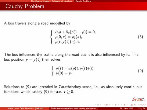
Cauchy Problem
A bus travels along a road modelled by ∂tρ+ ∂x (ρ(1− ρ)) = 0,ρ(0, x) = ρ0(x),ρ(t, y(t)) ≤ α.
(8)
The bus influences the traffic along the road but it is also influenced by it. Thebus position y = y(t) then solves
y(t) = ω(ρ(t, y(t)+)),y(0) = y0.
(9)
Solutions to (9) are intended in Caratheodory sense, i.e., as absolutely continuousfunctions which satisfy (9) for a.e. t ≥ 0.
Maria Laura Delle Monache (INRIA) Scalar conservation laws with moving constraints 28, June 2012 15 / 24
The Cauchy problem: Existence of solutions Cauchy Problem
Cauchy Problem: Solution
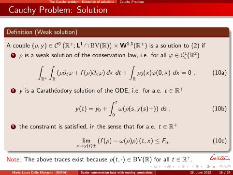
Definition (Weak solution)
A couple (ρ, y) ∈ C0(R+;L1 ∩ BV(R)
)×W1,1(R+) is a solution to (2) if
1 ρ is a weak solution of the conservation law, i.e. for all ϕ ∈ C1c (R2)∫
R+
∫R
(ρ∂tϕ+ f (ρ)∂xϕ) dx dt +
∫Rρ0(x)ϕ(0, x) dx = 0 ; (10a)
2 y is a Caratheodory solution of the ODE, i.e. for a.e. t ∈ R+
y(t) = y0 +
∫ t
0
ω(ρ(s, y(s)+)) ds ; (10b)
3 the constraint is satisfied, in the sense that for a.e. t ∈ R+
limx→y(t)±
(f (ρ)− ω(ρ)ρ) (t, x) ≤ Fα. (10c)
Note: The above traces exist because ρ(t, ·) ∈ BV(R) for all t ∈ R+.
Maria Laura Delle Monache (INRIA) Scalar conservation laws with moving constraints 28, June 2012 16 / 24
The Cauchy problem: Existence of solutions Wave-Front Tracking Method
Wave-Front Tracking Method I
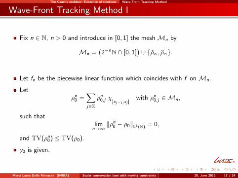
Fix n ∈ N, n > 0 and introduce in [0, 1] the mesh Mn by
Mn =(2−nN ∩ [0, 1]
)∪ ρα, ρα.
Let fn be the piecewise linear function which coincides with f on Mn.
Letρn
0 =∑j∈Z
ρn0,j χ]xj−1,xj ]
with ρn0,j ∈Mn,
such thatlim
n→∞‖ρn
0 − ρ0‖L1(R) = 0,
and TV(ρn0) ≤ TV(ρ0).
y0 is given.
Maria Laura Delle Monache (INRIA) Scalar conservation laws with moving constraints 28, June 2012 17 / 24
The Cauchy problem: Existence of solutions Wave-Front Tracking Method
Wave-Front Tracking Method II
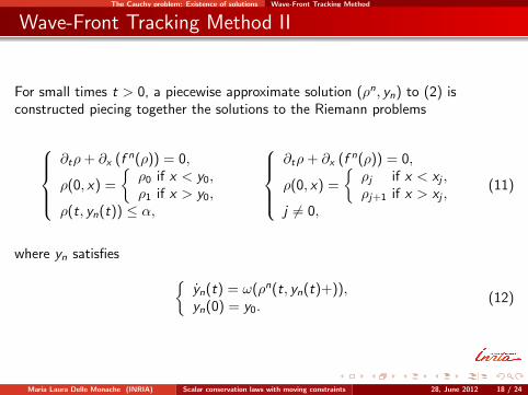
For small times t > 0, a piecewise approximate solution (ρn, yn) to (2) isconstructed piecing together the solutions to the Riemann problems
∂tρ+ ∂x (f n(ρ)) = 0,
ρ(0, x) =
ρ0 if x < y0,ρ1 if x > y0,
ρ(t, yn(t)) ≤ α,
∂tρ+ ∂x (f n(ρ)) = 0,
ρ(0, x) =
ρj if x < xj ,ρj+1 if x > xj ,
j 6= 0,
(11)
where yn satisfies yn(t) = ω(ρn(t, yn(t)+)),yn(0) = y0.
(12)
Maria Laura Delle Monache (INRIA) Scalar conservation laws with moving constraints 28, June 2012 18 / 24
The Cauchy problem: Existence of solutions Bounds on the total variation
Bounds on the total variation
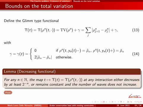
Define the Glimm type functional
Υ(t) = Υ(ρn(t, ·)) = TV(ρn) + γ =∑
j
∣∣ρnj+1 − ρn
j
∣∣+ γ, (13)
with
γ = γ(t) =
0 if ρn(t, yn(t)−) = ρα, ρn(t, yn(t)+) = ρα
2|ρα − ρα| otherwise.(14)
Lemma (Decreasing functional)
For any n ∈ N, the map t 7→ Υ(t) = Υ(ρn(t, ·)) at any interaction either decreasesby at least 2−n, or remains constant and the number of waves does not increase.
Proof
Maria Laura Delle Monache (INRIA) Scalar conservation laws with moving constraints 28, June 2012 19 / 24
The Cauchy problem: Existence of solutions Convergence of approximate solutions
Convergence of approximate solutions
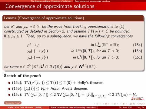
Lemma (Convergence of approximate solutions)
Let ρn and yn, n ∈ N, be the wave front tracking approximations to (1)constructed as detailed in Section 2, and assume TV(ρ0) ≤ C be bounded,0 ≤ ρ0 ≤ 1. Then, up to a subsequence, we have the following convergences
ρn → ρ in L1loc(R+ × R); (15a)
yn(·)→ y(·) in L∞([0,T ]), for all T > 0; (15b)
yn(·)→ y(·) in L1([0,T ]), for all T > 0; (15c)
for some ρ ∈ C0(R+;L1 ∩ BV(R)
)and y ∈W1,1(R+).
Sketch of the proof:
(15a): TV(ρn(t, ·)) ≤ Υ(t) ≤ Υ(0) + Helly’s theorem.
(15b): |yn(t)| ≤ Vb + Ascoli-Arzela theorem.
(15c): TV (yn; [0,T ]) ≤ 2 NV (yn; [0,T ]) + ‖yn‖L∞([0,T ]) ≤ 2TV(ρ0) + Vb
Complete Proof
Maria Laura Delle Monache (INRIA) Scalar conservation laws with moving constraints 28, June 2012 20 / 24
The Cauchy problem: Existence of solutions Existence of weak solution
Convergence of weak solution
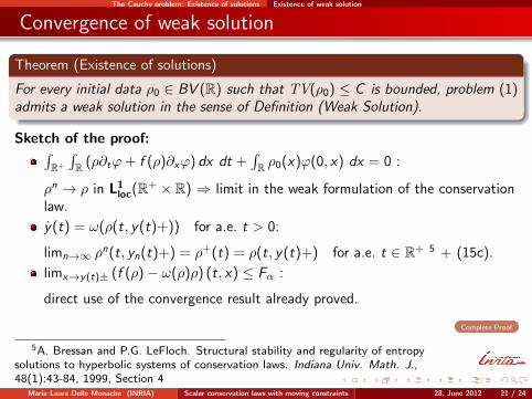
Theorem (Existence of solutions)
For every initial data ρ0 ∈ BV (R) such that TV(ρ0) ≤ C is bounded, problem (1)admits a weak solution in the sense of Definition (Weak Solution).
Sketch of the proof:∫R+
∫R (ρ∂tϕ+ f (ρ)∂xϕ) dx dt +
∫R ρ0(x)ϕ(0, x) dx = 0 :
ρn → ρ in L1loc(R+ × R) ⇒ limit in the weak formulation of the conservation
law.
y(t) = ω(ρ(t, y(t)+)) for a.e. t > 0:
limn→∞ ρn(t, yn(t)+) = ρ+(t) = ρ(t, y(t)+) for a.e. t ∈ R+ 5 + (15c).
limx→y(t)± (f (ρ)− ω(ρ)ρ) (t, x) ≤ Fα :
direct use of the convergence result already proved.
Complete Proof
5A. Bressan and P.G. LeFloch. Structural stability and regularity of entropysolutions to hyperbolic systems of conservation laws. Indiana Univ. Math. J.,48(1):43-84, 1999, Section 4
Maria Laura Delle Monache (INRIA) Scalar conservation laws with moving constraints 28, June 2012 21 / 24

Conclusions
Outline
1 IntroductionMathematical ModelExisting Models
2 The Riemann problem with moving density constraintRiemann ProblemRiemann Solver
3 The Cauchy problem: Existence of solutionsCauchy ProblemWave-Front Tracking MethodBounds on the total variationConvergence of approximate solutionsExistence of weak solution
4 Conclusions
Maria Laura Delle Monache (INRIA) Scalar conservation laws with moving constraints 28, June 2012 22 / 24

Conclusions
Conclusions and Future work
The coupled PDE-ODE model represents a good approach to the problem ofmoving bottleneck, as shown by different numerical approaches (works byF.Giorgi, J. Laval, L. Leclerq, C.F. Daganzo).
We were able to develop a strong coupling between the PDE and ODE.
We proved the existence of solutions for this model.
Stability of solution is currently a work in progress.
Maria Laura Delle Monache (INRIA) Scalar conservation laws with moving constraints 28, June 2012 23 / 24

Conclusions
Thank you for your attention.
Maria Laura Delle Monache (INRIA) Scalar conservation laws with moving constraints 28, June 2012 24 / 24
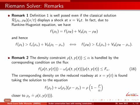
Riemann Solver: Remarks
Remark 1 Definition 1 is well posed even if the classical solutionR(ρL, ρR )(x/t) displays a shock at x = Vbt. In fact, due toRankine-Hugoniot equation, we have
f (ρL) = f (ρR ) + Vb(ρL − ρR )
and hence
f (ρL) > fα(ρα) + Vb(ρL − ρα) ⇐⇒ f (ρR ) > fα(ρα) + Vb(ρR − ρα).
Remark 2 The density constraint ρ(t, y(t)) ≤ α is handled by thecorresponding condition on the flux
f (ρ(t, y(t)))− ω(ρ(t, y(t)))ρ(t, y(t)) ≤ Fα. (16)
The corresponding density on the reduced roadway at x = y(t) is foundtaking the solution to the equation
f (ρy ) + ω(ρy )(ρ− ρy ) = ρ(
1− ρ
α
)closer to ρy
.= ρ(t, y(t))).
Back
Maria Laura Delle Monache (INRIA) Scalar conservation laws with moving constraints 28, June 2012 1 / 11
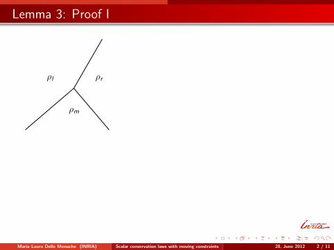
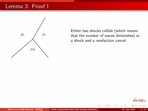
Lemma 3: Proof I
ρl ρr
ρm
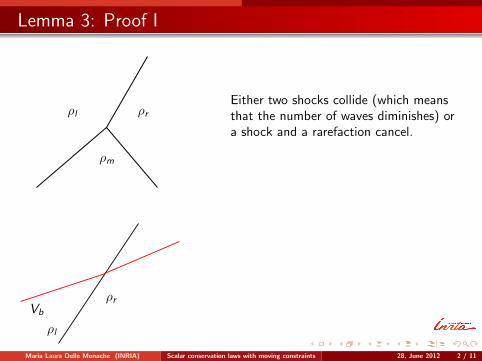
Either two shocks collide (which meansthat the number of waves diminishes) ora shock and a rarefaction cancel.
ρl
Vb
ρr
TV(ρn), Υ and the number of waves remainconstant.
Back
Maria Laura Delle Monache (INRIA) Scalar conservation laws with moving constraints 28, June 2012 2 / 11
Lemma 3: Proof I
ρl ρr
ρm
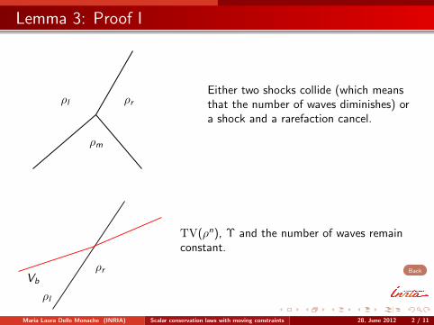
Either two shocks collide (which meansthat the number of waves diminishes) ora shock and a rarefaction cancel.
ρl
Vb
ρr
TV(ρn), Υ and the number of waves remainconstant.
Back
Maria Laura Delle Monache (INRIA) Scalar conservation laws with moving constraints 28, June 2012 2 / 11
Lemma 3: Proof I
ρl ρr
ρm
Either two shocks collide (which meansthat the number of waves diminishes) ora shock and a rarefaction cancel.
ρl
Vb
ρr
TV(ρn), Υ and the number of waves remainconstant.
Back
Maria Laura Delle Monache (INRIA) Scalar conservation laws with moving constraints 28, June 2012 2 / 11
Lemma 3: Proof II
ρα
ρα
ρl
Vb
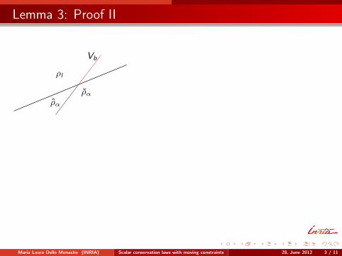
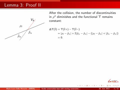
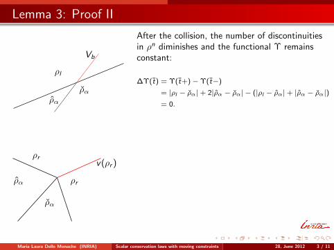
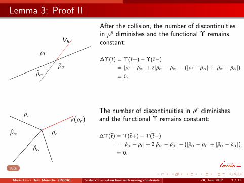
After the collision, the number of discontinuitiesin ρn diminishes and the functional Υ remainsconstant:
∆Υ(t) = Υ(t+)−Υ(t−)
= |ρl − ρα|+ 2|ρα − ρα| − (|ρl − ρα|+ |ρα − ρα|)= 0.
ρα
ρα
ρr
ρrv(ρr )
The number of discontinuities in ρn diminishesand the functional Υ remains constant:
∆Υ(t) = Υ(t+)−Υ(t−)
= |ρα − ρr |+ 2|ρα − ρα| − (|ρα − ρr |+ |ρα − ρα|)= 0.
Back
Maria Laura Delle Monache (INRIA) Scalar conservation laws with moving constraints 28, June 2012 3 / 11
Lemma 3: Proof II
ρα
ρα
ρl
Vb
After the collision, the number of discontinuitiesin ρn diminishes and the functional Υ remainsconstant:
∆Υ(t) = Υ(t+)−Υ(t−)
= |ρl − ρα|+ 2|ρα − ρα| − (|ρl − ρα|+ |ρα − ρα|)= 0.
ρα
ρα
ρr
ρrv(ρr )
The number of discontinuities in ρn diminishesand the functional Υ remains constant:
∆Υ(t) = Υ(t+)−Υ(t−)
= |ρα − ρr |+ 2|ρα − ρα| − (|ρα − ρr |+ |ρα − ρα|)= 0.
Back
Maria Laura Delle Monache (INRIA) Scalar conservation laws with moving constraints 28, June 2012 3 / 11
Lemma 3: Proof III
ρr = ρα
ρα
Vb
ρα
ρl
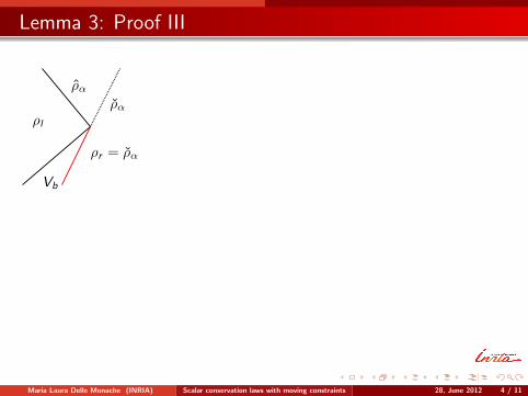
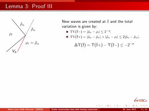
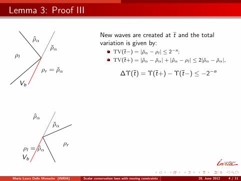
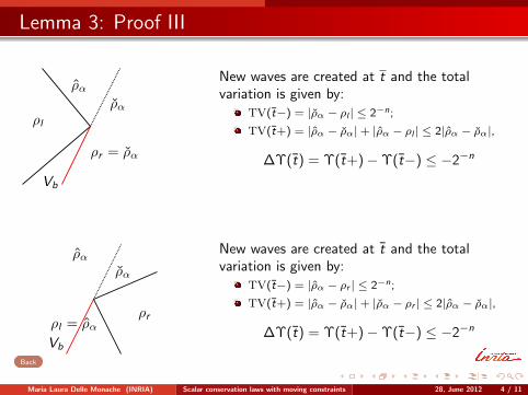
New waves are created at t and the totalvariation is given by:
TV(t−) = |ρα − ρl | ≤ 2−n;
TV(t+) = |ρα − ρα|+ |ρα − ρl | ≤ 2|ρα − ρα|,
∆Υ(t) = Υ(t+)−Υ(t−) ≤ −2−n
ρl = ρα
ρα
Vb
ρr
ρα
New waves are created at t and the totalvariation is given by:
TV(t−) = |ρα − ρr | ≤ 2−n;
TV(t+) = |ρα − ρα|+ |ρα − ρr | ≤ 2|ρα − ρα|,
∆Υ(t) = Υ(t+)−Υ(t−) ≤ −2−n
Back
Maria Laura Delle Monache (INRIA) Scalar conservation laws with moving constraints 28, June 2012 4 / 11
Lemma 3: Proof III
ρr = ρα
ρα
Vb
ρα
ρl
New waves are created at t and the totalvariation is given by:
TV(t−) = |ρα − ρl | ≤ 2−n;
TV(t+) = |ρα − ρα|+ |ρα − ρl | ≤ 2|ρα − ρα|,
∆Υ(t) = Υ(t+)−Υ(t−) ≤ −2−n
ρl = ρα
ρα
Vb
ρr
ρα
New waves are created at t and the totalvariation is given by:
TV(t−) = |ρα − ρr | ≤ 2−n;
TV(t+) = |ρα − ρα|+ |ρα − ρr | ≤ 2|ρα − ρα|,
∆Υ(t) = Υ(t+)−Υ(t−) ≤ −2−n
Back
Maria Laura Delle Monache (INRIA) Scalar conservation laws with moving constraints 28, June 2012 4 / 11
Convergence of approximate solutions II
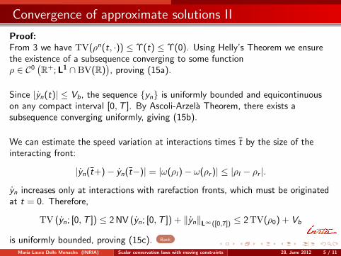
Proof:From 3 we have TV(ρn(t, ·)) ≤ Υ(t) ≤ Υ(0). Using Helly’s Theorem we ensurethe existence of a subsequence converging to some functionρ ∈ C0
(R+;L1 ∩ BV(R)
), proving (15a).
Since |yn(t)| ≤ Vb, the sequence yn is uniformly bounded and equicontinuouson any compact interval [0,T ]. By Ascoli-Arzela Theorem, there exists asubsequence converging uniformly, giving (15b).
We can estimate the speed variation at interactions times t by the size of theinteracting front:
|yn(t+)− yn(t−)| = |ω(ρl )− ω(ρr )| ≤ |ρl − ρr |.
yn increases only at interactions with rarefaction fronts, which must be originatedat t = 0. Therefore,
TV (yn; [0,T ]) ≤ 2 NV (yn; [0,T ]) + ‖yn‖L∞([0,7]) ≤ 2TV(ρ0) + Vb
is uniformly bounded, proving (15c). Back
Maria Laura Delle Monache (INRIA) Scalar conservation laws with moving constraints 28, June 2012 5 / 11
Convergence of weak solution I
∫R+
∫R
(ρ∂tϕ+ f (ρ)∂xϕ) dx dt +
∫Rρ0(x)ϕ(0, x) dx = 0 ; (17)
Proof:Since ρn converge strongly to ρ in L1
loc(R+ × R), it is straightforward to pass tothe limit in the weak formulation of the conservation law, proving that the limitfunction ρ satisfies (17).
y(t) = ω(ρ(t, y(t)+)) for a. e.t > 0. (18)
Proof:We prove that
limn→∞
ρn(t, yn(t)+) = ρ+(t) = ρ(t, y(t)+) for a. e. t ∈ R+. (19)
By pointwise convergence a. e. of ρn to ρ, ∃ a sequence zn ≥ yn(t) s.t. zn → y(t)and ρn(t, zn)→ ρ+(t).
Back
Maria Laura Delle Monache (INRIA) Scalar conservation laws with moving constraints 28, June 2012 6 / 11
Convergence of weak solution II
Cont.
For a. e. t > 0, the point (t, y(t)) is for ρ(t, ·) either a continuity point, or itbelongs to a discontinuity curve (either a classical or a non-classical shock ).
Fix ε∗ > 0 and assume TV (ρ(t, ·); ]y(t)− δ, y(t) + δ[) ≤ ε∗, for some δ > 0.
Then by weak convergence of measure6 TV (ρn(t, ·); ]y(t)− δ, y(t) + δ[) ≤ 2ε∗
for n large enough, and∣∣ρn(t, yn(t)+)− ρ+(t)∣∣ ≤ |ρn(t, yn(t)+)− ρn(t, zn)|+
∣∣ρn(t, zn)− ρ+(t)∣∣ ≤ 3ε∗
for n large enough.
If ρ(t, ·) has a discontinuity of strength greater than ε∗ at y(t), then|ρn(t, yn(t)+)− ρn(t, yn(t)−)| ≥ ε∗/2 for n sufficiently large.
Back
6Lemma 15, A. Bressan and P.G. LeFloch. Structural stability and regularity ofentropy solutions to hyperbolic systems of conservation laws. Indiana Univ. Math.J.,48(1):43-84, 1999
Maria Laura Delle Monache (INRIA) Scalar conservation laws with moving constraints 28, June 2012 7 / 11

Convergence of weak solution III
Cont.
We set ρn,+ = ρn(t, yn(t)+) and we show that for each ε > 0 there exists δ > 0such that for all n large enough there holds∣∣ρn(s, x)− ρn,+
∣∣ < ε for |s − t| ≤ δ, |x − y(t)| ≤ δ, x > yn(s). (20)
In fact, if (20) does not hold, we could find ε > 0 and sequences tn → t, δn → 0s. t. TV (ρn(tn, ·); ]yn(tn), yn(tn) + δn[) ≥ ε.
By strict concavity of the flux function f , there should be a uniformly positiveamount of interactions in an arbitrarily small neighborhood of (t, y(t)), giving acontradiction. Therefore (20) holds and we get∣∣ρn(t, yn(t)+)− ρ+(t)
∣∣ ≤ |ρn(t, yn(t)+)− ρn(t, zn)|+∣∣ρn(t, zn)− ρ+(t)
∣∣ ≤ 2ε
for n large enough, thus proving (19).Combining (15c) and (19) we get (18).
Back
Maria Laura Delle Monache (INRIA) Scalar conservation laws with moving constraints 28, June 2012 8 / 11
Convergence of weak solution IV
limx→y(t)±
(f (ρ)− ω(ρ)ρ) (t, x) ≤ Fα. (21)
Proof:
Introduce the setsΩ± = (t, x) ∈ R+ × R : x ≶ y(t)
andΩ±n = (t, x) ∈ R+ × R : x ≶ yn(t),
Consider a test function ϕ ∈ C1c (R+ × R), ϕ ≥ 0, s. t.
supp(ϕ) ∩ (t, y(t)) : t > 0 6= 0 and supp(ϕ) ∩ (t, yn(t)) : t > 0 6= 0.
Back
Maria Laura Delle Monache (INRIA) Scalar conservation laws with moving constraints 28, June 2012 9 / 11
Convergence of weak solution V
Cont.
Then by conservation on Ω+n we have∫∫
χΩ+n
(ρn∂tϕ+ f n(ρn)∂xϕ
)dx dt
=
∫ +∞
0
∫ +∞
yn(t)
(ρn∂tϕ+ f n(ρn)∂xϕ
)dx dt
=
∫ +∞
0
(f n(ρn(t, yn(t)+))− yn(t)ρn(t, yn(t)+)
)ϕ(t, yn(t)) dt
=
∫ +∞
0
(f n(ρn(t, yn(t)+))− ω(ρn(t, yn(t)+))ρn(t, yn(t)+)
)ϕ(t, yn(t)) dt
≤∫ T
0
Fαϕ(t, yn(t)) dt, (22)
Back
Maria Laura Delle Monache (INRIA) Scalar conservation laws with moving constraints 28, June 2012 10 / 11

Convergence of weak solution VI
Cont.
The same can be done for the limit solutions ρ and y(t) that, by conservation onΩ, satisfy∫∫
χΩ+
(ρ∂tϕ+ f (ρ)∂xϕ
)dx dt =
∫ +∞
0
∫ +∞
y(t)
(ρ∂tϕ+ f (ρ)∂xϕ
)dx dt
=
∫ +∞
0
(f (ρ(t, y(t)+))− y(t)ρ(t, y(t)+)
)ϕ(t, y(t)) dt
=
∫ +∞
0
(f (ρ(t, y(t)+))− ω(ρ(t, y(t)+))ρ(t, y(t)+)
)ϕ(t, y(t)) dt (23)
By (15a) and (15b) we can pass to the limit in (22) and (23), which gives∫ +∞
0
(f (ρ(t, y(t)+))− ω(ρ(t, y(t)+))ρ(t, y(t)+)− Fα
)ϕ(t, y(t)) dt ≤ 0.
Since the above inequality holds for every test function ϕ ≥ 0,we have proved (21).
Back
Maria Laura Delle Monache (INRIA) Scalar conservation laws with moving constraints 28, June 2012 11 / 11