Scalable training of L1-regularizedlog-linear models

Galen Andrew(Joint work with Jianfeng Gao)

ICML, 2007

Minimizing regularized loss

• Many parametric ML models are trained by minimizing a regularized loss of the form:

• is a loss function quantifying “fit to the data”– Negative log-likelihood of training data– Distance from decision boundary of incorrect examples

• If zero is a reasonable “default” parameter value, we can use where is a norm, penalizing large vectors, and C is a constant

Types of norms

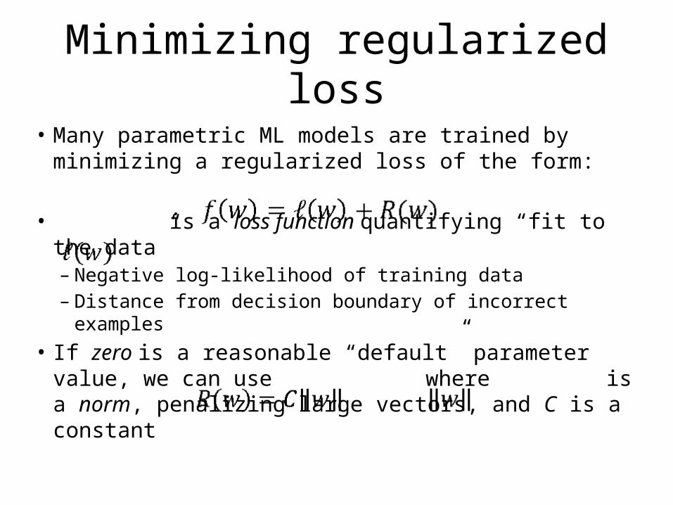
• A norm precisely defines “size” of a vector

2

1

3

Contours of L2-norm in 2D Contours of L1-norm in 2D

123

A nice property of L1

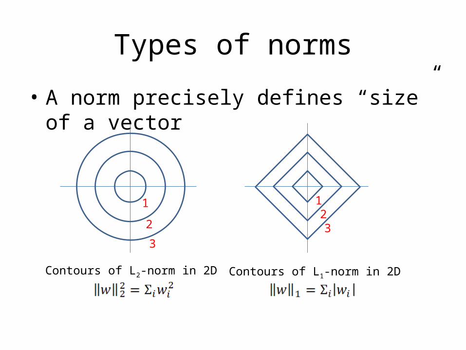
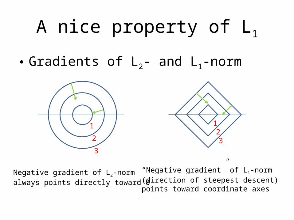
• Gradients of L2- and L1-norm

2

1

3

123

Negative gradient of L2-norm always points directly toward 0

“Negative gradient” of L1-norm (direction of steepest descent)points toward coordinate axes

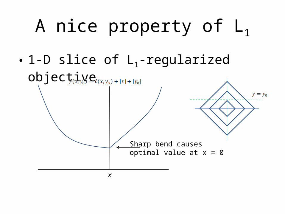
A nice property of L1

• 1-D slice of L1-regularized objective

Sharp bend causes optimal value at x = 0

x

A nice property of L1

• At global optimum, many parameters have value exactly zero– L2 would give small, nonzero values

• Thus L1 does continuous feature selection– More interpretable, computationally manageable

models• C parameter tunes sparsity/accuracy tradeoff• In our experiments, only 1.5% of feats remain

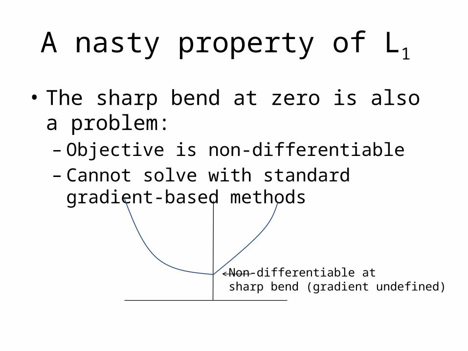
A nasty property of L1

• The sharp bend at zero is also a problem:– Objective is non-differentiable– Cannot solve with standard gradient-based

methods

Non-differentiable atsharp bend (gradient undefined)

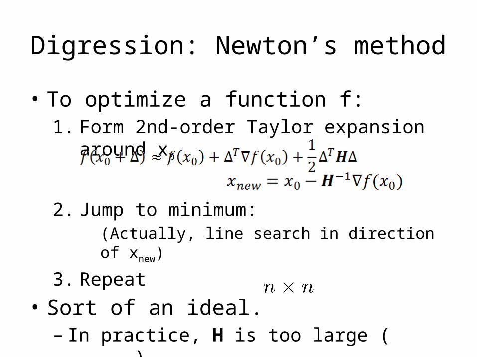
Digression: Newton’s method

• To optimize a function f:1. Form 2nd-order Taylor expansion around x0

2. Jump to minimum:(Actually, line search in direction of xnew)

3. Repeat• Sort of an ideal.– In practice, H is too large ( )

Limited-Memory Quasi-Newton

• Approximate H-1 with a low-rank matrix built using information from recent iterations– Approximate H-1 and not H, so no need to invert

the matrix or solve linear system!• Most popular L-M Q-N method: L-BFGS– Storage and computation are O(# vars)– Very good theoretical convergence properties– Empirically, best method for training large-scale

log-linear models with L2 (Malouf ‘02, Minka ‘03)

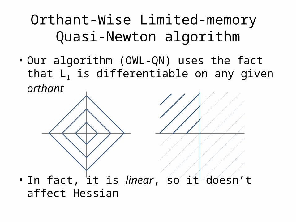
• Our algorithm (OWL-QN) uses the fact that L1 is differentiable on any given orthant

• In fact, it is linear, so it doesn’t affect Hessian

Orthant-Wise Limited-memory Quasi-Newton algorithm

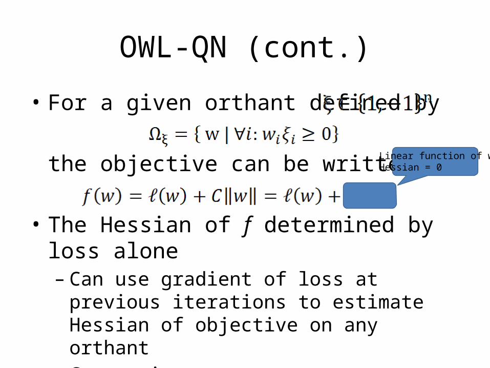
• For a given orthant defined by

the objective can be written

• The Hessian of f determined by loss alone– Can use gradient of loss at previous iterations to

estimate Hessian of objective on any orthant– Constrain steps to not cross orthant boundaries

OWL-QN (cont.)

Linear function of wHessian = 0

OWL-QN (cont.)

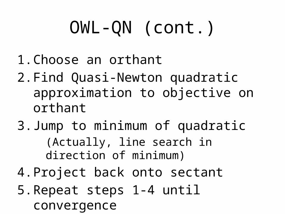
1. Choose an orthant2. Find Quasi-Newton quadratic approximation

to objective on orthant3. Jump to minimum of quadratic

(Actually, line search in direction of minimum)

4. Project back onto sectant5. Repeat steps 1-4 until convergence

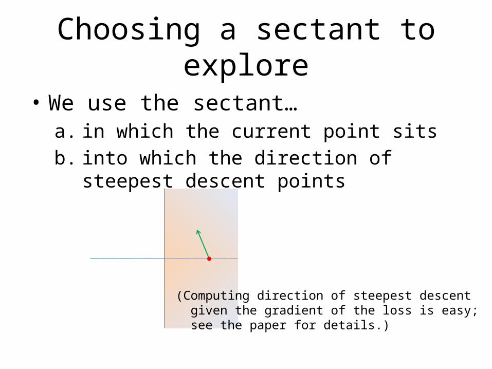
Choosing a sectant to explore

• We use the sectant…a. in which the current point sitsb. into which the direction of steepest descent

points

(Computing direction of steepest descent given the gradient of the loss is easy; see the paper for details.)

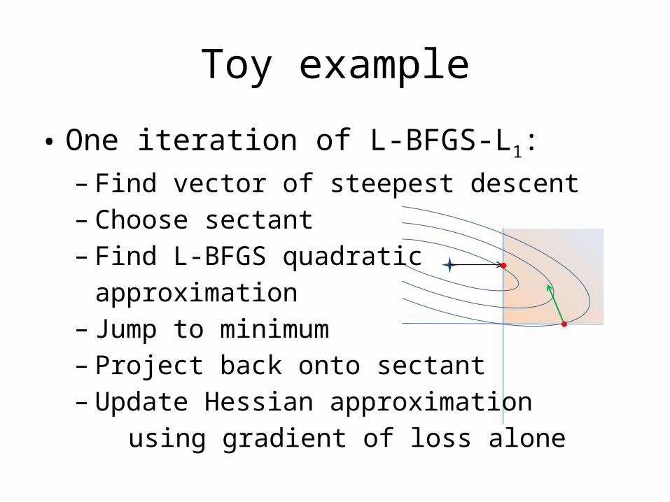
Toy example

• One iteration of L-BFGS-L1:– Find vector of steepest descent– Choose sectant– Find L-BFGS quadratic

approximation– Jump to minimum– Project back onto sectant– Update Hessian approximation

using gradient of loss alone

Notes

• Variables added/subtracted from model as orthant boundaries are hit

• A variable can change signs in two iterations• Glossing over some details:– Line search with projection at each iteration– Convenient for implementation to expand notion

of “orthant” to constrain some variables at zero– See paper for complete details

• In paper we prove convergence to optimum

Experiments

• We ran experiments with the parse re-ranking model of Charniak & Johnson (2005)– Start with a set of candidate parses for each

sentence (produced by a baseline parser)– Train a log-linear model to select the correct one

• Model uses ~1.2M features of a parse• Train on Sections 2-19 of PTB (36K sentences

with 50 parses each)• Fit C to max. F-meas on Sec. 20-21 (4K sent.)

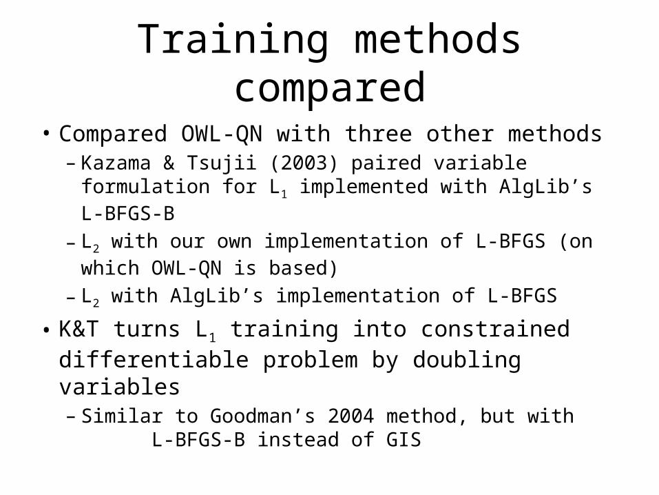
Training methods compared

• Compared OWL-QN with three other methods– Kazama & Tsujii (2003) paired variable formulation for

L1 implemented with AlgLib’s L-BFGS-B

– L2 with our own implementation of L-BFGS (on which OWL-QN is based)

– L2 with AlgLib’s implementation of L-BFGS

• K&T turns L1 training into constrained differentiable problem by doubling variables– Similar to Goodman’s 2004 method, but with L-

BFGS-B instead of GIS

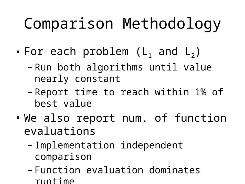
Comparison Methodology

• For each problem (L1 and L2)– Run both algorithms until value nearly constant– Report time to reach within 1% of best value

• We also report num. of function evaluations– Implementation independent comparison– Function evaluation dominates runtime

• Results reported with chosen value of C• L-BFGS memory parameter = 5 for all runs

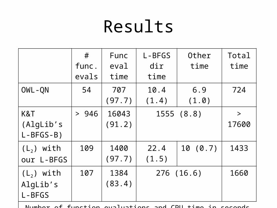
Results# func. evals

Func eval time

L-BFGS dir time

Other time Total time

OWL-QN 54 707 (97.7)

10.4 (1.4) 6.9 (1.0) 724

K&T (AlgLib’s L-BFGS-B)

> 946 16043 (91.2)

1555 (8.8) > 17600

(L2) withour L-BFGS

109 1400 (97.7)

22.4 (1.5) 10 (0.7) 1433

(L2) withAlgLib’s L-BFGS

107 1384 (83.4)

276 (16.6) 1660

Number of function evaluations and CPU time in seconds to reach within 1% of best value found. Figures in parentheses are percentage of total time.

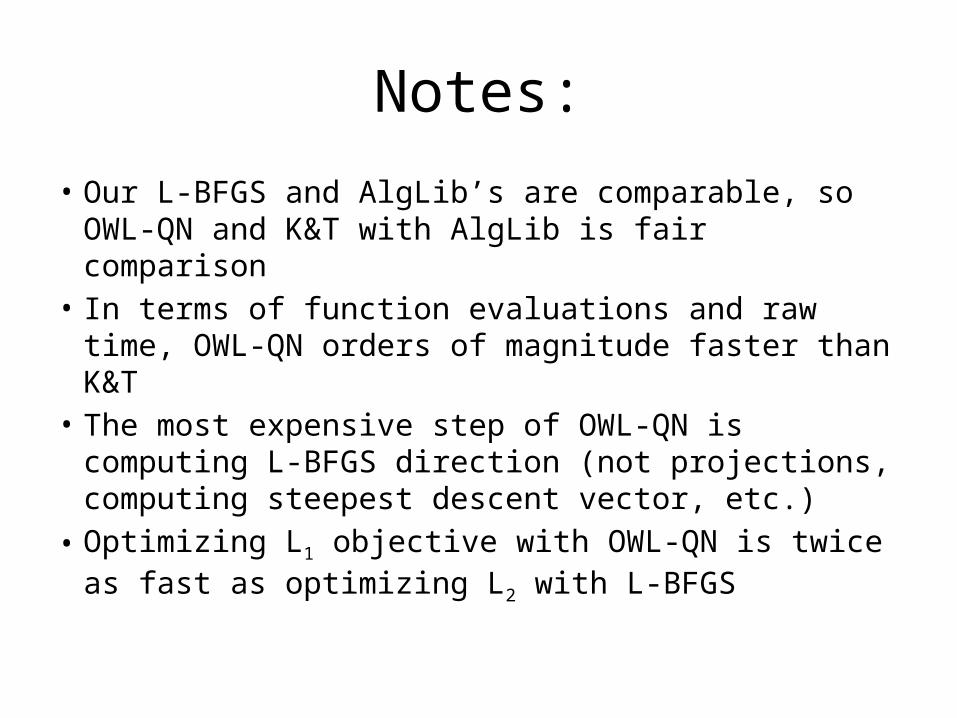
Notes:

• Our L-BFGS and AlgLib’s are comparable, so OWL-QN and K&T with AlgLib is fair comparison

• In terms of function evaluations and raw time, OWL-QN orders of magnitude faster than K&T

• The most expensive step of OWL-QN is computing L-BFGS direction (not projections, computing steepest descent vector, etc.)

• Optimizing L1 objective with OWL-QN is twice as fast as optimizing L2 with L-BFGS

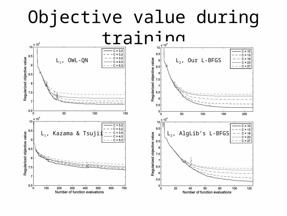
Objective value during training

L2, Our L-BFGS

L2, AlgLib’s L-BFGSL1, Kazama & Tsujii

L1, OWL-QN

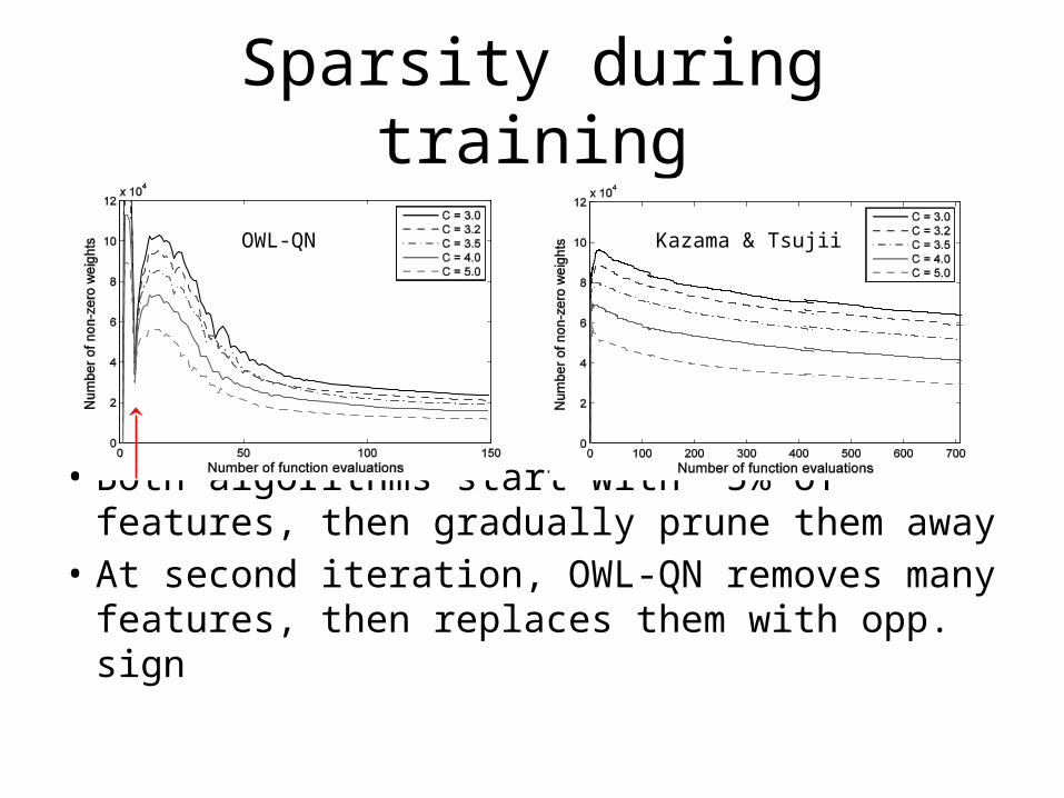
• Both algorithms start with ~5% of features, then gradually prune them away

• At second iteration, OWL-QN removes many features, then replaces them with opp. sign

Sparsity during training

OWL-QN Kazama & Tsujii

Extensions

• For ACL paper, ran on 3 very different log-linear NLP models with up to 8M features– CMM sequence model for POS tagging– Reranking log-linear model for LM adaptation– Semi-CRF for Chinese word segmentation

• Can use any smooth convex loss– We’ve also tried least-squares (LASSO regression)

• A small change allows non-convex loss– Only local minimum guaranteed

Software download

• We’ve released c++ OWL-QN source– User can specify arbitrary convex smooth loss

• Also included are standalone trainer for L1 logistic regression and least-squares (LASSO)

• Please visit my webpage for download– (Find with search engine of your choice)

THANKS.