Scalable Recognition with a Vocabulary Tree

David Nister and Henrik Stewenius

Center for Visualization and Virtual Environments

Department of Computer Science, University of Kentucky

http://www.vis.uky.edu/∼dnister/ http://www.vis.uky.edu/∼stewe/

Abstract

A recognition scheme that scales efficiently to a large

number of objects is presented. The efficiency and quality is

exhibited in a live demonstration that recognizes CD-covers

from a database of 40000 images of popular music CD’s.

The scheme builds upon popular techniques of indexing

descriptors extracted from local regions, and is robust

to background clutter and occlusion. The local region

descriptors are hierarchically quantized in a vocabulary

tree. The vocabulary tree allows a larger and more

discriminatory vocabulary to be used efficiently, which we

show experimentally leads to a dramatic improvement in

retrieval quality. The most significant property of the

scheme is that the tree directly defines the quantization. The

quantization and the indexing are therefore fully integrated,

essentially being one and the same.

The recognition quality is evaluated through retrieval

on a database with ground truth, showing the power of

the vocabulary tree approach, going as high as 1 million

images.

1. Introduction

Object recognition is one of the core problems in

computer vision, and it is a very extensively investigated

topic. Due to appearance variabilities caused for

example by non-rigidity, background clutter, differences in

viewpoint, orientation, scale or lighting conditions, it is a

hard problem.

One of the important challenges is to construct methods

that scale well with the size of the database, and can select

one out of a large number of objects in acceptable time. In

this paper, a method handling a large number of objects is

presented. The approach belongs to a currently very popular

class of algorithms that work with local image regions and

This work was supported in part by the National Science Foundation

under award number IIS-0545920, Faculty Early Career Development

(CAREER) Program.

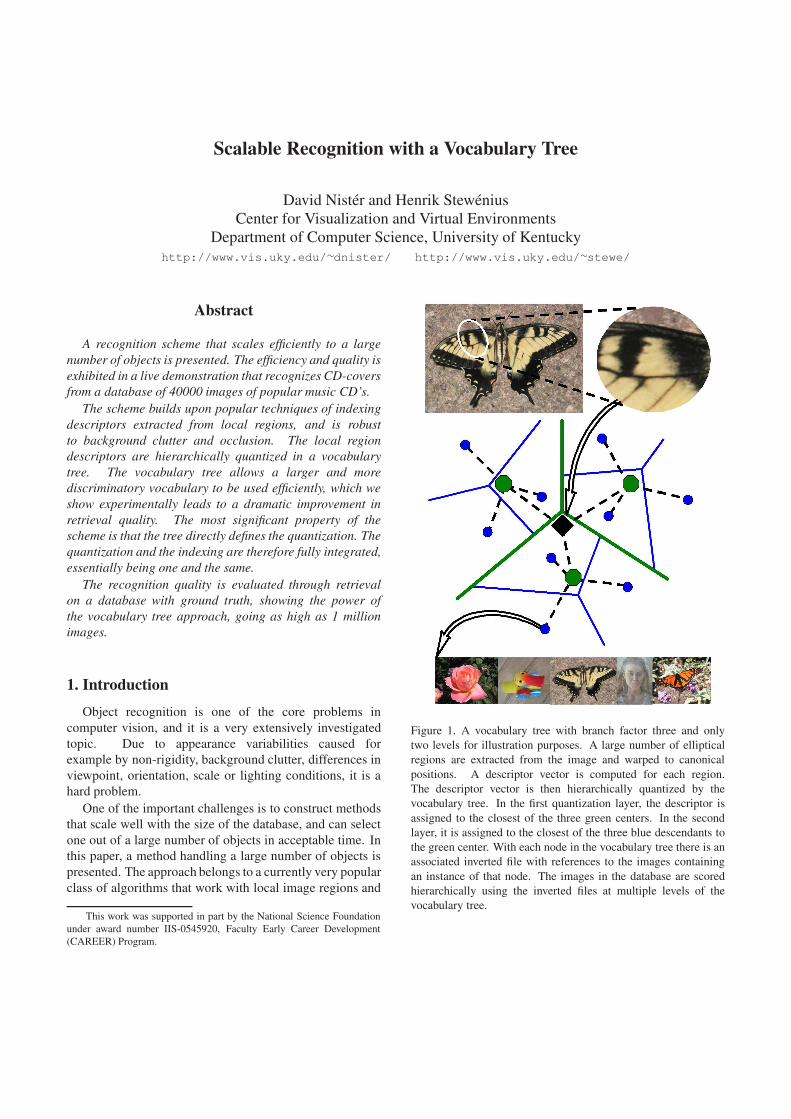
Figure 1. A vocabulary tree with branch factor three and only

two levels for illustration purposes. A large number of elliptical

regions are extracted from the image and warped to canonical

positions. A descriptor vector is computed for each region.

The descriptor vector is then hierarchically quantized by the

vocabulary tree. In the first quantization layer, the descriptor is

assigned to the closest of the three green centers. In the second

layer, it is assigned to the closest of the three blue descendants to

the green center. With each node in the vocabulary tree there is an

associated inverted file with references to the images containing

an instance of that node. The images in the database are scored

hierarchically using the inverted files at multiple levels of the

vocabulary tree.

represent an object with descriptors extracted from these

local regions [1, 2, 8, 11, 15, 16, 18]. The strength of this

class of algorithms is natural robustness against occlusion

and background clutter.

The most important contribution of this paper is

an indexing mechanism that enables extremely efficient

retrieval. In the current implementation of the proposed

scheme, feature extraction on a 640 × 480 video frame

takes around 0.2 seconds and the database query takes

25ms on a database with 50000 images.

2. Approach and its Relation to Previous Work

Our work is largely inspired by Sivic and Zisserman

[17]. They perform retrieval of shots from a movie using

a text retrieval approach. Descriptors extracted from local

affine invariant regions are quantized into visual words,

which are defined by k-means performed on the descriptor

vectors from a number of training frames. The collection of

visual words are used in Term Frequency Inverse Document

Frequency (TF-IDF) scoring of the relevance of an image to

the query. The scoring is accomplished using inverted files.

We propose a hierarchical TF-IDF scoring using

hierarchically defined visual words that form a vocabulary

tree. This allows much more efficient lookup of visual

words, which enables the use of a larger vocabulary, which

is shown to result in a significant improvement of retrieval

quality. In particular, we show high quality retrieval

results without any consideration of the geometric layout

of visual words within the frame, while [17] reports that the

geometric layout is crucial for retrieval quality, which we

also find to be true when using a smaller vocabulary. We

will concentrate on showing the quality of the pre-geometry

stage of retrieval, which we believe is important in order to

scale up to large databases.

The recognition quality is evaluated through retrieval on

a database with ground truth consisting of known groups of

images of the same object or location, but under different

viewpoint, rotation, scale and lighting conditions. This

evaluation shows that the vocabulary tree allows us to

achieve significantly better than previous methods, both in

terms of quality and efficiency.

The use of a larger vocabulary also unleashes the

true power of the inverted file approach by decreasing

the fraction of images in the database that have to be

explicitly considered. In [17], a vocabulary with on the

order of 10000 visual words are used. With on the

order of 1000 visual words per frame, this means that

approximately a tenth of the database is traversed during a

query, even if the occupancy of visual words in the database

is uniformly distributed. We show that better retrieval

quality is obtained with a larger vocabulary, even as large

as a vocabulary tree with 16 million leaf nodes. With

this size of vocabulary, several orders of magnitude less

features from the database have to be explicitly considered.

Thus both higher retrieval quality and efficiency is obtained.

In particular, we obtain sub-second retrieval times for a

database of a million images, while in [17], only on the

order of a few thousand frames was attempted. We use

hierarchical scoring, meaning that other nodes than the leaf

nodes are considered, but the number of images attached

to the inverted file of a node are limited to a fixed number,

since larger inverted files are expensive and provide little

entropy in the TF-IDF scoring.

The vocabulary tree also provides more efficient training

by using a hierarchical k-means approach. In [17], 400

training frames are used, while here we go as high as 35000,

which we show improves the quality when using a large

vocabulary.

While [17] uses an offline crawling stage to index the

video, which takes at least 10 seconds per frame, we can

insert images into the database at the same rate as reported

for the feature extraction, i.e. around 5Hz for 640 × 480resolution. This potential for on-the-fly insertion of new

objects into the database is a result of the quantization into

visual words, which is defined once and for all, while still

allowing general high retrieval performance. This feature

is important, but rather uncommon in previous work. We

plan to use it for vision-based simultaneous localization and

mapping, where new locations need to be added on-the-fly.

Several authors have shown that trees present an efficient

way to index local image regions. For example, Lepetit,

Lagger and Fua [7] use re-rendering of image patches

to train multiple decision trees that are used to index

keypoints, somewhat reminiscent of locality sensitive

hashing [6, 3]. The measurements used in their trees are

ratios of pixel intensities. In contrast, we use proximity of

the descriptor vectors to various cluster centers defining the

vocabulary tree. Their method provides very fast online

operation. It is focused on detection of a single object,

but could potentially be used for more objects. With their

method, training optimally for a new object takes 10-15

minutes, and their fastest method takes one minute for

training a new object. We use an offline unsupervised

training stage to define the vocabulary tree, but once the

vocabulary tree is determined, new images can be inserted

on-the-fly into the database.

Decision trees are also used by Obdrzalek and Matas

[14] to index keypoints. They use pixel measurements, each

aimed at splitting the descriptor distribution roughly in half.

They have shown online recognition of on the order of 100

to 1000 objects with this method. Insertion of new objects

requires offline training of the decision tree.

Lowe [9] uses a k-d tree with a best-bin-first

modification to find approximate nearest neighbors to the

descriptor vectors of the query. Lowe presents results with

up to around 100000 keypoint descriptors in the database,

which with the cited number of 2000 stable features per

frame amounts to about 50 training images in the database.

Lowe’s approach has been used on around 5000 objects

in a commercial application, but we are not aware of an

academic reference describing these results.

For the most part, the above approaches keep amounts

of data around in the database that is on the order of

magnitude as large as the image patches themselves, or

at least the region descriptors. However, the compactness

of the database is very important for query efficiency in

a large database. With our vocabulary tree approach, the

representation of an image patch is simply one or two

integers, which should be contrasted to the hundreds of

bytes or floats used for a descriptor vector.

Compactness is also the most important difference

between our approach and the hierarchical approach used

by Grauman and Darrell [5]. They use a pyramid of

histograms, at each level doubling the number of bins along

each axis without considering the distribution of data. By

using a vocabulary adapted to the likely distribution of

data, we can use a much smaller tree, resulting in better

resolution while maintaining a compact representation. We

also estimate that our approach is around a factor 1000

faster.

For feature extraction, we use our own implementation

of Maximally Stable Extremal Regions (MSERs) [10].

They have been found to perform well in thorough

performance evaluation [13, 4]. We warp an elliptical

patch around each MSER region into a circular patch.

The remaining portion of our feature extraction is then

implemented according to the SIFT feature extraction

pipeline by Lowe [9]. Canonical directions are found based

on an orientation histogram formed on the image gradients.

SIFT descriptors are then extracted relative to the canonical

directions. The SIFT descriptors have been found highly

distinctive in performance evaluation [12]. The normalized

SIFT descriptors are then quantized with the vocabulary

tree. Finally, a hierarchical scoring scheme is applied to

retrieve images from a database.

3. Building and Using the Vocabulary Tree

The vocabulary tree defines a hierarchical quantization

that is built by hierarchical k-means clustering. A large

set of representative descriptor vectors are used in the

unsupervised training of the tree.

Instead of k defining the final number of clusters or

quantization cells, k defines the branch factor (number of

children of each node) of the tree. First, an initial k-

means process is run on the training data, defining k cluster

centers. The training data is then partitioned into k groups,

where each group consists of the descriptor vectors closest

to a particular cluster center.

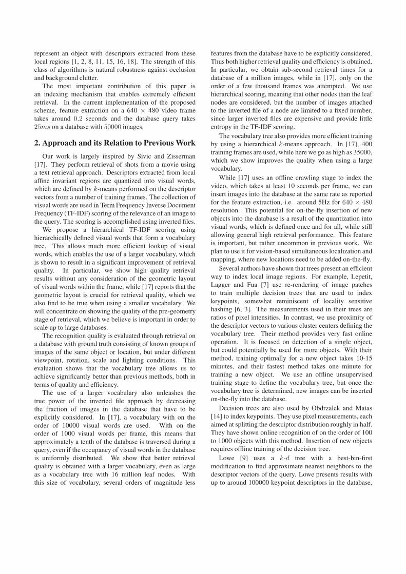
The same process is then recursively applied to

Figure 2. An illustration of the process of building the vocabulary

tree. The hierarchical quantization is defined at each level by k

centers (in this case k = 3) and their Voronoi regions.

each group of descriptor vectors, recursively defining

quantization cells by splitting each quantization cell into k

new parts. The tree is determined level by level, up to some

maximum number of levels L, and each division into k parts

is only defined by the distribution of the descriptor vectors

that belong to the parent quantization cell. The process is

illustrated in Figure 2.

In the online phase, each descriptor vector is simply

propagated down the tree by at each level comparing

the descriptor vector to the k candidate cluster centers

(represented by k children in the tree) and choosing the

closest one. This is a simple matter of performing k

dot products at each level, resulting in a total of kL dot

products, which is very efficient if k is not too large. The

path down the tree can be encoded by a single integer and

is then available for use in scoring.

Note that the tree directly defines the visual vocabulary

and an efficient search procedure in an integrated

manner. This is different from for example defining a

visual vocabulary non-hierarchically, and then devising

an approximate nearest neighbor search in order to find

visual words efficiently. We find the seamless choice

more appealing, although the latter approach also defines

quantization cells in the original space if used consistently

and deterministically. The hierarchical approach also gives

more flexibility to the subsequent scoring procedure.

While the computational cost of increasing the size of

the vocabulary in a non-hierarchical manner would be very

high, the computational cost in the hierarchical approach is

logarithmic in the number of leaf nodes. The memory usage

is linear in the number of leaf nodes kL. The total number

of descriptor vectors that must be represented is∑L

i=1ki =

kL+1−kk−1

≈ kL. For D-dimensional descriptors represented

as char the size of the tree is approximately DkL bytes.

With our current implementation, a tree with D = 128, L =6 and k = 10, resulting in 1M leaf nodes, uses 143MB of

memory.

4. Definition of Scoring

Once the quantization is defined, we wish to determine

the relevance of a database image to the query image based

on how similar the paths down the vocabulary tree are

for the descriptors from the database image and the query

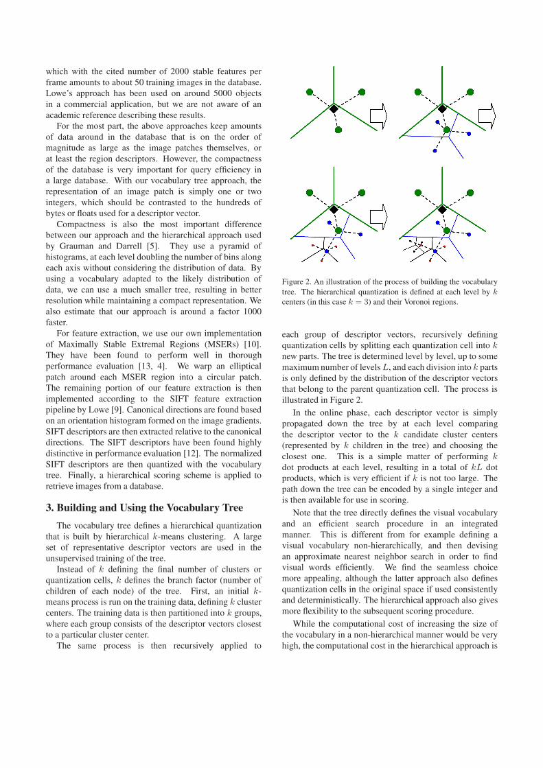
image. An illustration of this representation of an image is

given in Figure 3. There is a myriad of options here, and we

have compared a number of variants empirically.

Most of the schemes we have tried can be thought of as

assigning a weight wi to each node i in the vocabulary tree,

typically based on entropy, and then define both query qi

and database vectors di according to the assigned weights

as

qi = niwi (1)

di = miwi (2)

where ni and mi are the number of descriptor vectors of the

query and database image, respectively, with a path through

node i. A database image is then given a relevance score s

based on the normalized difference between the query and

database vectors:

s(q, d) =‖q

‖ q ‖−

d

‖ d ‖‖ . (3)

The normalization can be in any desired norm and is used

to achieve fairness between database images with few and

many descriptor vectors. We have found that L1-norm gives

better results than the more standard L2-norm.

In the simplest case, the weights wi are set to a constant,

but retrieval performance is typically improved by an

entropy weighting like

wi = lnN

Ni

, (4)

where N is the number of images in the database, and Ni

is the number of images in the database with at least one

descriptor vector path through node i. This results in a TF-

IDF scheme. We have also tried to use the frequency of

occurrence of node i in place of Ni, but it seems not to

make much difference.

The weights for the different levels of the vocabulary tree

can be handled in various ways. Intuitively, it seems correct

Figure 3. Three levels of a vocabulary tree with branch factor 10

populated to represent an image with 400 features.

to assign the entropy of each node relative to the node above

it in the path, but we have, perhaps somewhat surprisingly,

found that it is better to use the entropy relative to the root of

the tree and ignore dependencies within the path. It is also

possible to block some of the levels in the tree by setting

their weights to zero and only use the levels closest to the

leaves.

We have found that most important for the retrieval

quality is to have a large vocabulary (large number of leaf

nodes), and not give overly strong weights to the inner

nodes of the vocabulary tree. In principle, the vocabulary

size must eventually grow too large, so that the variability

and noise in the descriptor vectors frequently move the

descriptor vectors between different quantization cells.

The trade-off here is of course distinctiveness (requiring

small quantization cells and a deep vocabulary tree) versus

repeatability (requiring large quantization cells). However,

a benefit of hierarchical scoring is that the risk of overdoing

the size of the vocabulary is lessened. Moreover, we

have found that for a large range of vocabulary sizes (up

to somewhere between 1 and 16 million leaf nodes), the

retrieval performance increases with the number of leaf

nodes. This is probably also the explanation to why it is

better to assign entropy directly relative to the root node.

The leaf nodes are simply much more powerful than the

inner nodes.

It is also possible to use stop lists, where wi is set

to zero for the most frequent and/or infrequent symbols.

When using inverted files, we block the longer lists. This

can be done since symbols in very densely populated lists

do not contribute much entropy. We do this mainly to

retain efficiency, but it sometimes even improves retrieval

performance. Stop lists were indicated in [17] to remove

mismatches from the correspondence set. However, in most

cases we have not been able to improve retrieval quality by

using stop lists.

5. Implementation of Scoring

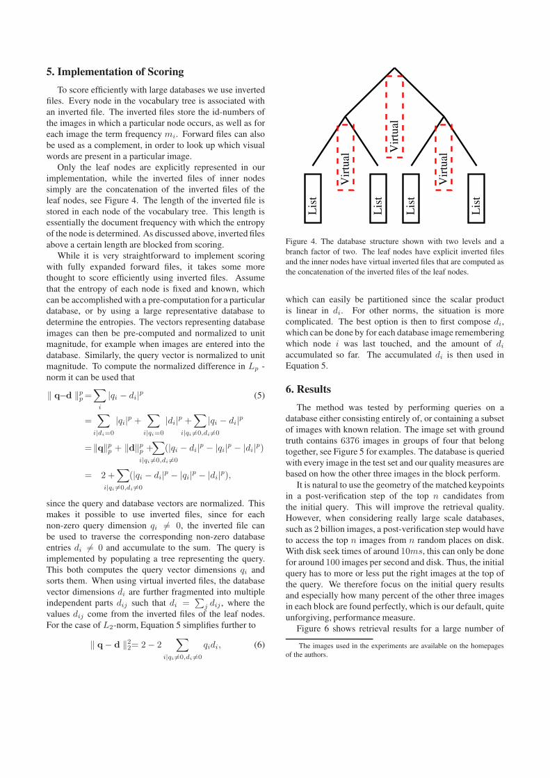
To score efficiently with large databases we use inverted

files. Every node in the vocabulary tree is associated with

an inverted file. The inverted files store the id-numbers of

the images in which a particular node occurs, as well as for

each image the term frequency mi. Forward files can also

be used as a complement, in order to look up which visual

words are present in a particular image.

Only the leaf nodes are explicitly represented in our

implementation, while the inverted files of inner nodes

simply are the concatenation of the inverted files of the

leaf nodes, see Figure 4. The length of the inverted file is

stored in each node of the vocabulary tree. This length is

essentially the document frequency with which the entropy

of the node is determined. As discussed above, inverted files

above a certain length are blocked from scoring.

While it is very straightforward to implement scoring

with fully expanded forward files, it takes some more

thought to score efficiently using inverted files. Assume

that the entropy of each node is fixed and known, which

can be accomplished with a pre-computation for a particular

database, or by using a large representative database to

determine the entropies. The vectors representing database

images can then be pre-computed and normalized to unit

magnitude, for example when images are entered into the

database. Similarly, the query vector is normalized to unit

magnitude. To compute the normalized difference in Lp -

norm it can be used that

‖ q−d ‖pp =

∑

i

|qi − di|p (5)

=∑

i|di=0

|qi|p +

∑

i|qi=0

|di|p +

∑

i|qi 6=0,di 6=0

|qi − di|p

=‖q‖pp + ‖d‖p

p +∑

i|qi 6=0,di 6=0

(|qi − di|p − |qi|

p − |di|p)

= 2 +∑

i|qi 6=0,di 6=0

(|qi − di|p − |qi|

p − |di|p),

since the query and database vectors are normalized. This

makes it possible to use inverted files, since for each

non-zero query dimension qi 6= 0, the inverted file can

be used to traverse the corresponding non-zero database

entries di 6= 0 and accumulate to the sum. The query is

implemented by populating a tree representing the query.

This both computes the query vector dimensions qi and

sorts them. When using virtual inverted files, the database

vector dimensions di are further fragmented into multiple

independent parts dij such that di =∑

j dij , where the

values dij come from the inverted files of the leaf nodes.

For the case of L2-norm, Equation 5 simplifies further to

‖ q − d ‖2

2= 2 − 2

∑

i|qi 6=0,di 6=0

qidi, (6)

Lis

t

Lis

t

Lis

t

Lis

t

Vir

tual

Vir

tual

Vir

tual

Figure 4. The database structure shown with two levels and a

branch factor of two. The leaf nodes have explicit inverted files

and the inner nodes have virtual inverted files that are computed as

the concatenation of the inverted files of the leaf nodes.

which can easily be partitioned since the scalar product

is linear in di. For other norms, the situation is more

complicated. The best option is then to first compose di,

which can be done by for each database image remembering

which node i was last touched, and the amount of di

accumulated so far. The accumulated di is then used in

Equation 5.

6. Results

The method was tested by performing queries on a

database either consisting entirely of, or containing a subset

of images with known relation. The image set with ground

truth contains 6376 images in groups of four that belong

together, see Figure 5 for examples. The database is queried

with every image in the test set and our quality measures are

based on how the other three images in the block perform.

It is natural to use the geometry of the matched keypoints

in a post-verification step of the top n candidates from

the initial query. This will improve the retrieval quality.

However, when considering really large scale databases,

such as 2 billion images, a post-verification step would have

to access the top n images from n random places on disk.

With disk seek times of around 10ms, this can only be done

for around 100 images per second and disk. Thus, the initial

query has to more or less put the right images at the top of

the query. We therefore focus on the initial query results

and especially how many percent of the other three images

in each block are found perfectly, which is our default, quite

unforgiving, performance measure.

Figure 6 shows retrieval results for a large number of

The images used in the experiments are available on the homepages

of the authors.

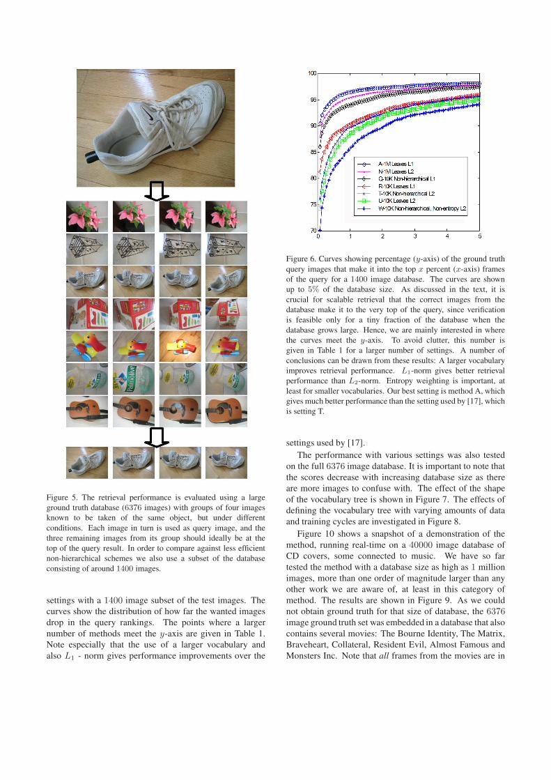
Figure 5. The retrieval performance is evaluated using a large

ground truth database (6376 images) with groups of four images

known to be taken of the same object, but under different

conditions. Each image in turn is used as query image, and the

three remaining images from its group should ideally be at the

top of the query result. In order to compare against less efficient

non-hierarchical schemes we also use a subset of the database

consisting of around 1400 images.

settings with a 1400 image subset of the test images. The

curves show the distribution of how far the wanted images

drop in the query rankings. The points where a larger

number of methods meet the y-axis are given in Table 1.

Note especially that the use of a larger vocabulary and

also L1 - norm gives performance improvements over the

Figure 6. Curves showing percentage (y-axis) of the ground truth

query images that make it into the top x percent (x-axis) frames

of the query for a 1400 image database. The curves are shown

up to 5% of the database size. As discussed in the text, it is

crucial for scalable retrieval that the correct images from the

database make it to the very top of the query, since verification

is feasible only for a tiny fraction of the database when the

database grows large. Hence, we are mainly interested in where

the curves meet the y-axis. To avoid clutter, this number is

given in Table 1 for a larger number of settings. A number of

conclusions can be drawn from these results: A larger vocabulary

improves retrieval performance. L1-norm gives better retrieval

performance than L2-norm. Entropy weighting is important, at

least for smaller vocabularies. Our best setting is method A, which

gives much better performance than the setting used by [17], which

is setting T.

settings used by [17].

The performance with various settings was also tested

on the full 6376 image database. It is important to note that

the scores decrease with increasing database size as there

are more images to confuse with. The effect of the shape

of the vocabulary tree is shown in Figure 7. The effects of

defining the vocabulary tree with varying amounts of data

and training cycles are investigated in Figure 8.

Figure 10 shows a snapshot of a demonstration of the

method, running real-time on a 40000 image database of

CD covers, some connected to music. We have so far

tested the method with a database size as high as 1 million

images, more than one order of magnitude larger than any

other work we are aware of, at least in this category of

method. The results are shown in Figure 9. As we could

not obtain ground truth for that size of database, the 6376image ground truth set was embedded in a database that also

contains several movies: The Bourne Identity, The Matrix,

Braveheart, Collateral, Resident Evil, Almost Famous and

Monsters Inc. Note that all frames from the movies are in

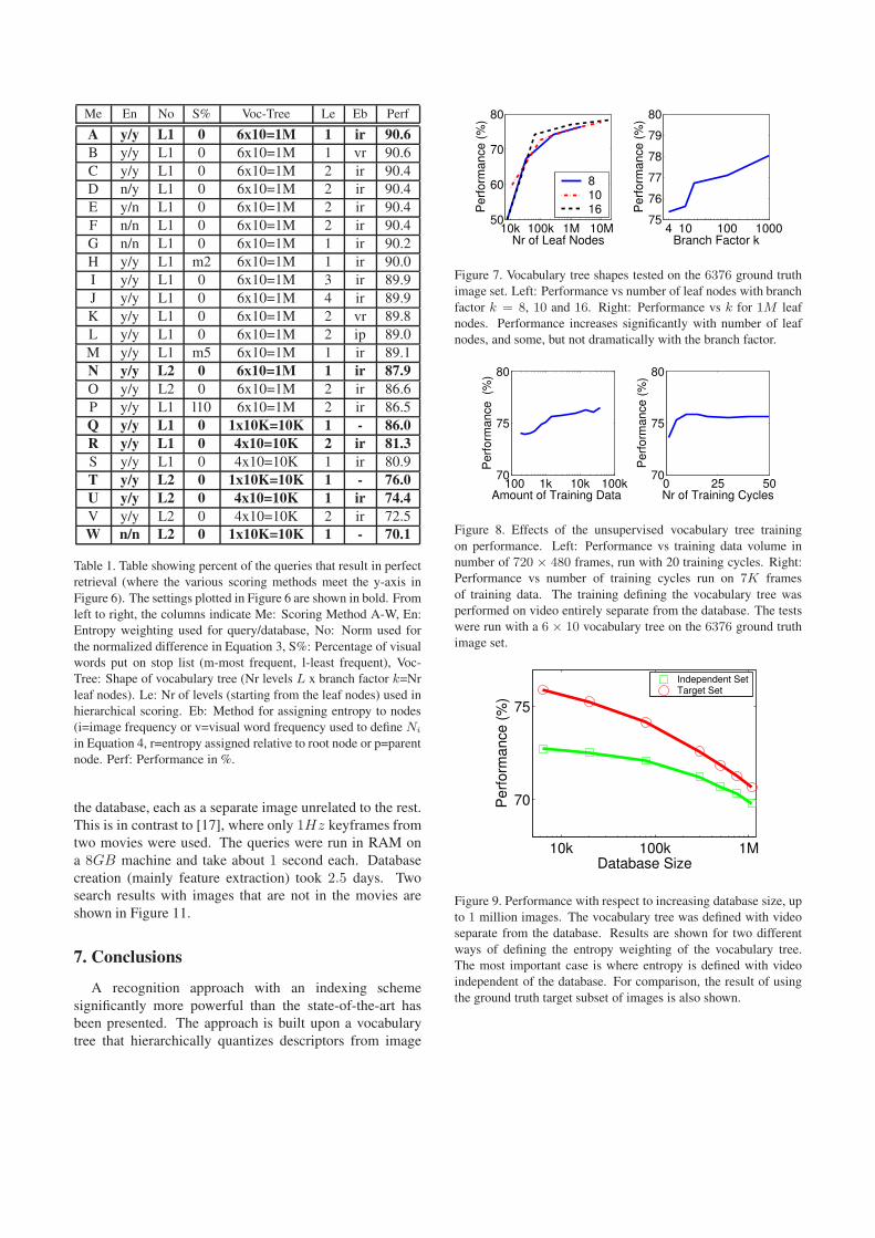
Me En No S% Voc-Tree Le Eb Perf

A y/y L1 0 6x10=1M 1 ir 90.6

B y/y L1 0 6x10=1M 1 vr 90.6

C y/y L1 0 6x10=1M 2 ir 90.4

D n/y L1 0 6x10=1M 2 ir 90.4

E y/n L1 0 6x10=1M 2 ir 90.4

F n/n L1 0 6x10=1M 2 ir 90.4

G n/n L1 0 6x10=1M 1 ir 90.2

H y/y L1 m2 6x10=1M 1 ir 90.0

I y/y L1 0 6x10=1M 3 ir 89.9

J y/y L1 0 6x10=1M 4 ir 89.9

K y/y L1 0 6x10=1M 2 vr 89.8

L y/y L1 0 6x10=1M 2 ip 89.0

M y/y L1 m5 6x10=1M 1 ir 89.1

N y/y L2 0 6x10=1M 1 ir 87.9

O y/y L2 0 6x10=1M 2 ir 86.6

P y/y L1 l10 6x10=1M 2 ir 86.5

Q y/y L1 0 1x10K=10K 1 - 86.0

R y/y L1 0 4x10=10K 2 ir 81.3

S y/y L1 0 4x10=10K 1 ir 80.9

T y/y L2 0 1x10K=10K 1 - 76.0

U y/y L2 0 4x10=10K 1 ir 74.4

V y/y L2 0 4x10=10K 2 ir 72.5

W n/n L2 0 1x10K=10K 1 - 70.1

Table 1. Table showing percent of the queries that result in perfect

retrieval (where the various scoring methods meet the y-axis in

Figure 6). The settings plotted in Figure 6 are shown in bold. From

left to right, the columns indicate Me: Scoring Method A-W, En:

Entropy weighting used for query/database, No: Norm used for

the normalized difference in Equation 3, S%: Percentage of visual

words put on stop list (m-most frequent, l-least frequent), Voc-

Tree: Shape of vocabulary tree (Nr levels L x branch factor k=Nr

leaf nodes). Le: Nr of levels (starting from the leaf nodes) used in

hierarchical scoring. Eb: Method for assigning entropy to nodes

(i=image frequency or v=visual word frequency used to define Ni

in Equation 4, r=entropy assigned relative to root node or p=parent

node. Perf: Performance in %.

the database, each as a separate image unrelated to the rest.

This is in contrast to [17], where only 1Hz keyframes from

two movies were used. The queries were run in RAM on

a 8GB machine and take about 1 second each. Database

creation (mainly feature extraction) took 2.5 days. Two

search results with images that are not in the movies are

shown in Figure 11.

7. Conclusions

A recognition approach with an indexing scheme

significantly more powerful than the state-of-the-art has

been presented. The approach is built upon a vocabulary

tree that hierarchically quantizes descriptors from image

10k 100k 1M 10M50

60

70

80

Pe

rfo

rma

nce

(%

)

Nr of Leaf Nodes

81016

4 10 100 100075

76

77

78

79

80

Pe

rfo

rma

nce

(%

)

Branch Factor k

Figure 7. Vocabulary tree shapes tested on the 6376 ground truth

image set. Left: Performance vs number of leaf nodes with branch

factor k = 8, 10 and 16. Right: Performance vs k for 1M leaf

nodes. Performance increases significantly with number of leaf

nodes, and some, but not dramatically with the branch factor.

100 1k 10k 100k70

75

80

Perf

orm

ance (%

)Amount of Training Data

0 25 5070

75

80

Perf

orm

ance (

%)

Nr of Training Cycles

Figure 8. Effects of the unsupervised vocabulary tree training

on performance. Left: Performance vs training data volume in

number of 720 × 480 frames, run with 20 training cycles. Right:

Performance vs number of training cycles run on 7K frames

of training data. The training defining the vocabulary tree was

performed on video entirely separate from the database. The tests

were run with a 6 × 10 vocabulary tree on the 6376 ground truth

image set.

10k 100k 1M

70

75

Pe

rfo

rma

nce

(%

)

Database Size

Independent SetTarget Set

Figure 9. Performance with respect to increasing database size, up

to 1 million images. The vocabulary tree was defined with video

separate from the database. Results are shown for two different

ways of defining the entropy weighting of the vocabulary tree.

The most important case is where entropy is defined with video

independent of the database. For comparison, the result of using

the ground truth target subset of images is also shown.

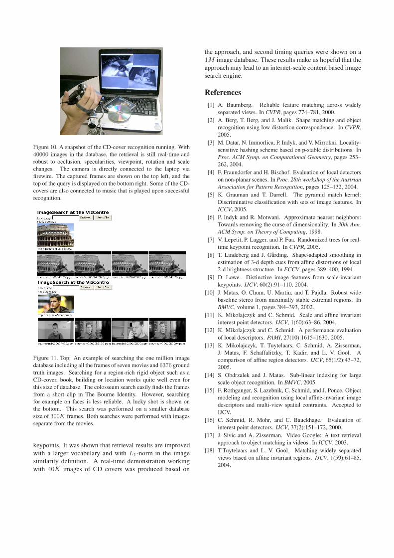
Figure 10. A snapshot of the CD-cover recognition running. With

40000 images in the database, the retrieval is still real-time and

robust to occlusion, specularities, viewpoint, rotation and scale

changes. The camera is directly connected to the laptop via

firewire. The captured frames are shown on the top left, and the

top of the query is displayed on the bottom right. Some of the CD-

covers are also connected to music that is played upon successful

recognition.

Figure 11. Top: An example of searching the one million image

database including all the frames of seven movies and 6376 ground

truth images. Searching for a region-rich rigid object such as a

CD-cover, book, building or location works quite well even for

this size of database. The colosseum search easily finds the frames

from a short clip in The Bourne Identity. However, searching

for example on faces is less reliable. A lucky shot is shown on

the bottom. This search was performed on a smaller database

size of 300K frames. Both searches were performed with images

separate from the movies.

keypoints. It was shown that retrieval results are improved

with a larger vocabulary and with L1-norm in the image

similarity definition. A real-time demonstration working

with 40K images of CD covers was produced based on

the approach, and second timing queries were shown on a

1M image database. These results make us hopeful that the

approach may lead to an internet-scale content based image

search engine.

References

[1] A. Baumberg. Reliable feature matching across widely

separated views. In CVPR, pages 774–781, 2000.

[2] A. Berg, T. Berg, and J. Malik. Shape matching and object

recognition using low distortion correspondence. In CVPR,

2005.

[3] M. Datar, N. Immorlica, P. Indyk, and V. Mirrokni. Locality-

sensitive hashing scheme based on p-stable distributions. In

Proc. ACM Symp. on Computational Geometry, pages 253–

262, 2004.

[4] F. Fraundorfer and H. Bischof. Evaluation of local detectors

on non-planar scenes. In Proc. 28th workshop of the Austrian

Association for Pattern Recognition, pages 125–132, 2004.

[5] K. Grauman and T. Darrell. The pyramid match kernel:

Discriminative classification with sets of image features. In

ICCV, 2005.

[6] P. Indyk and R. Motwani. Approximate nearest neighbors:

Towards removing the curse of dimensionality. In 30th Ann.

ACM Symp. on Theory of Computing, 1998.

[7] V. Lepetit, P. Lagger, and P. Fua. Randomized trees for real-

time keypoint recognition. In CVPR, 2005.

[8] T. Lindeberg and J. Garding. Shape-adapted smoothing in

estimation of 3-d depth cues from affine distortions of local

2-d brightness structure. In ECCV, pages 389–400, 1994.

[9] D. Lowe. Distinctive image features from scale-invariant

keypoints. IJCV, 60(2):91–110, 2004.

[10] J. Matas, O. Chum, U. Martin, and T. Pajdla. Robust wide

baseline stereo from maximally stable extremal regions. In

BMVC, volume 1, pages 384–393, 2002.

[11] K. Mikolajczyk and C. Schmid. Scale and affine invariant

interest point detectors. IJCV, 1(60):63–86, 2004.

[12] K. Mikolajczyk and C. Schmid. A performance evaluation

of local descriptors. PAMI, 27(10):1615–1630, 2005.

[13] K. Mikolajczyk, T. Tuytelaars, C. Schmid, A. Zisserman,

J. Matas, F. Schaffalitzky, T. Kadir, and L. V. Gool. A

comparison of affine region detectors. IJCV, 65(1/2):43–72,

2005.

[14] S. Obdrzalek and J. Matas. Sub-linear indexing for large

scale object recognition. In BMVC, 2005.

[15] F. Rothganger, S. Lazebnik, C. Schmid, and J. Ponce. Object

modeling and recognition using local affine-invariant image

descriptors and multi-view spatial contraints. Accepted to

IJCV.

[16] C. Schmid, R. Mohr, and C. Bauckhage. Evaluation of

interest point detectors. IJCV, 37(2):151–172, 2000.

[17] J. Sivic and A. Zisserman. Video Google: A text retrieval

approach to object matching in videos. In ICCV, 2003.

[18] T.Tuytelaars and L. V. Gool. Matching widely separated

views based on affine invariant regions. IJCV, 1(59):61–85,

2004.