Scalable Parallel Graph Algorithms with Matrix-Vector ...ordonez/pdf/j-mat-vec.pdf · works and hyper-link real data sets, we present performance comparisons between a columnar DBMS,

Noname manuscript No.(will be inserted by the editor)

Scalable Parallel Graph Algorithms withMatrix-Vector Multiplication Evaluated with Queries

Wellington Cabrera · Carlos Ordonez

Received: date / Accepted: date

Abstract Graph problems are significantly harder to solve with large graphs re-siding on disk compared to main memory only. In this work, we study how tosolve four important graph problems: reachability from a source vertex, singlesource shortest path, weakly connected components, and PageRank. It is wellknown that the aforementioned algorithms can be expressed as an iteration ofmatrix-vector multiplications under different semi-rings. Based on this mathemat-ical foundation, we show how to express the computation with standard relationalqueries and then we study how to efficiently evaluate them in parallel in a shared-nothing architecture. We identify a common algorithmic pattern that unifies thefour graph algorithms, considering a common mathematical foundation based onsparse matrix-vector multiplication. The net gain is that our SQL-based approachenables solving ”big data” graph problems on parallel database systems, debunk-ing common wisdom that they are cumbersome and slow. Using large social net-works and hyper-link real data sets, we present performance comparisons betweena columnar DBMS, an open-source array DBMS, and Spark’s GraphX.

Keywords Graph · parallel computation · data distribution · Columnar DBMS ·Array DBMS

1 Introduction

Graph analytics is a field which is increasing its importance every day. Further-more, as the world has become more interconnected than before, graph data setsare larger and more complex. In graph analytics, the goal is to obtain insight andunderstanding of complex relationships that are present in telecommunication,transportation and social networks. In general, real-life graphs are sparse. While

Wellington CabreraUniversity of HoustonE-mail: [email protected]

Carlos OrdonezUniversity of HoustonE-mail: [email protected]

2 Wellington Cabrera, Carlos Ordonez

there are more than one billion user accounts in Facebook, a typical user may beconnected just to a few hundred contacts. Other examples are roads connectingcities and flights linking airports. In this work, we concentrate on algorithms forsparse graphs stored in parallel DBMSs.

Relational database systems remain the most common technology to storetransactions and analytical data, due to optimized I/O, robustness and securitycontrol. Even though, the common understanding is that RDBMSs cannot han-dle demanding graph problems, because relational queries are not sufficient toexpress important graphs algorithms, and a poor performance of database en-gines in the context of graph analytics. Consequently, several graph databases andgraphs analytics systems have emerged, targeting large data sets, especially un-der the Hadoop/MapReduce platform. In recent years, Pregel and its open-sourcesuccessor Giraph have supported the ”vertex-centric” approach. This approach isbased on performing computations at the vertex scope and sending/receiving mes-sages to/from its neighbors. On the other hand, the ”algebraic approach” solvesgraph algorithms via a generalized matrix multiplication, generally with optimizedprograms running in clusters with large main memory.

Why in-database Graph Analytics

DBMSs are between the most widespread systems in the industry. It is hard toimagine how to run an organization without using DBMSs, in any industrial field.Moreover, most of the internet relies on DBMSs for social networking, dynamiccontent or electronic commerce. Therefore, a lot of data is stored in these systems.We believe that efficient graph algorithms for relational databases are a contri-bution that will support in-database graphs analytics in large data sets, avoidingwasting time exporting the data or setting up external systems.

Summary of Contributions

In this work we show how to compute several graph algorithms in a parallel DBMS,by executing iteratively one elegant (yet efficient) relational query. In contrast topopular graph analytics systems, our algorithms are able to process data sets largerthan the main memory, since they are conceived as external algorithms. We presenta unified algorithm based on regular relational queries with join-aggregationto solve classic graph problems, such as Reachability from a source vertex, Sin-gle Source Shortest Paths, Connected Components, and PageRank. We explain agraph partitioning strategy which reduces the execution time of the parallel queriesof our unified algorithm, by improving data locality and avoiding redundant data.While a general optimization of graph queries is out the scope of this work, weshow experimentally that by using optimized join-aggregation queries, parallelDBMSs can compute a family of fundamental graph algorithms with promisingperformance. Furthermore, we show that columnar and array DBMSs are compet-itive to a state-of-the art system, namely Spark-GraphX.

Parallel Graph Algorithms with In-database Matrix-Vector Multiplication 3

2 Related Work

In the last years the problem of solving graph algorithms in parallel DBMS withrelational queries has received limited attention. Recently, the authors of [14]studied Vertica as a platform for graph analytics, focusing in the conversion ofvertex-centric programs to relational queries, and in the implementation of shared-memory graph processing via UDFs, in one node. [26] describes the enhancementsto SAP HANA to support graph analytics, in a columnar in-memory database. In[31], the authors show that their SQL implementation of shortest path algorithmhas better performance than Neo4j. Note that the later work runs in one nodewith a large RAM (1 TB). Running on top of Hadoop, Pegasus[16] is a graphsystem based on matrix multiplications; the authors propose grouping the cells ofthe matrix in blocks, to increase performance in a large-RAM cluster. Pregelix [3]is another graph system, built on top of the Hyracks parallel dataflow engine; theauthors report better performance than GraphX, claiming that this system brings”data-parallel query evaluation techniques from the database world”. Our workis different from the previously described in several ways: 1) we present a unifiedframework for compute graph algorithms with relational queries; 2) we present op-timizations for columnar and array DBMSs based on a careful data distribution;3) the out-of-core graph computation allows us to analyze graphs with hundredsmillions edges with minimum RAM requirements.

A sub-problem of sparse-matrix vector multiplication is analyzed in [25]. Specif-ically, the authors propose an array-relation dot-product join database operator,motivated by the computation of Stochastic Gradient Descent (SGD). Regard-ing the matrix-vector multiplication with relational operators, the authors argueabout its applicability to SGD. In contrast, our work is focused on the optimiza-tion of graph algorithms. The algorithms of our concern do not require incrementalupdates; instead, the matrix vector multiplication updates completely the results.While our algorithms do not require gradient methods, it would be interesting tostudy if the dot product operator could be applicable to graph problems.

In our initial work [21], we proposed optimized recursive queries to solve twoimportant graph problems using SQL: Transitive closure and All Pairs ShortestPath. Our recent work [22] shows that columnar DBMS technology performs muchbetter than array or row DBMSs. More recently, we turned our attention to graphalgorithms based on matrix-vector multiplication with relational queries in [4],where we explored a unified algorithm to solve several graph problems. However,DBMS storage details, parallelism, and query optimizations were not studied.

3 Definitions and Background

3.1 Graph Dataset

Let G = (V,E) be a directed graph, where V is a set of vertices and E is a set ofedges, considered as an ordered pairs of vertices. Let n = |V | vertices and m = |E|edges. The adjacency matrix of G is a n× n matrix such that the cell i, j holds a1 when exists an edge from vertex i to vertex j. In order to simplify notation, wedenote as E the adjacency matrix of G. The outdegree of a vertex v is the numberof outgoing edges of v and the indegree of v is the number of incoming edges of v.


The algorithms in this work use a vector S to store the output and intermediateresults. The ith entry of S is a value corresponding to vertex i, and it is denotedas S[i].

Graph Storage

In sparse graphs processing, it is reasonable to represent the adjacency matrix of Gin a sparse form, which saves storage and computing resources. There exist severalmechanisms to represent sparse matrices, and the interested reader may check [2].In our work, sparse matrices are represented as a set of tuples (i, j, v) such thatv 6= 0, where i and j represent row/column, and v represents the value of entryEij . Since cells where v = 0 are not stored, the space complexity is m = |E|. Insparse matrices, we assume m = O(n)

3.2 Parallel Systems Overview

The algorithms in this work are conceived for parallel DBMSs under a shared-nothing architecture. While our optimized algorithms can work in any DBMS, inour previous work [22], we showed experimentally that columnar and array DBMSspresent performance substantially better than row DBMSs for graphs analysis. Forthis reason we concentrate the study in columnar and array DBMSs. These systemsare architected for fast query processing, rather than transaction processing. Inthis work, we consider parallel DBMSs running in a cluster with N nodes.

Row DBMS

The pioneer parallel database management systems stored data by rows. Thissystems were aimed to exploit the I/O bandwidth of multiple disks [7], improvingin this way reading and writing performance, and allowing the storage of datatoo big to fit in only one machine. Large tables are to be partitioned throughthe parallel system. Three common methods of partitioning are: 1) splitting thetables to the nodes by ranges with respect to an attribute’s value; 2) distributingrecords to the nodes in a round-robin assignment; 3) using a hash function toassign records to the nodes. Currently, the last method is the most commonlyused.

Columnar DBMSs

Columnar DBMSs emerged in the previous decade presenting outstanding perfor-mance for OLAP. C-Store [29] and Monet-DB [12] are among the first systemsthat have exploited the columnar storage. Columnar DBMSs can evaluate queriesfaster than traditional row-oriented DBMSs, specially queries with join or aggre-gation operations. While row DBMSs generally store data in blocks containing aset of records, columnar DBMSs store columns in separate files, as large blocks ofcontiguous data. Storing data by column benefit the use of compression. Due tothe low entropy of the data in a column, low-overhead data compression has beenexploited for further performance improvements. This data compression does not


hinder parallelism. Columnar DBMS indexing is significantly different than tradi-tional row stores. For instance, in Vertica there is no row-level index defined by theDBA. Instead, additional projections can be defined to improve query execution.An in-depth study of columnar DBMS architectures is given in [1].

Array DBMSs

Array store is a technology aimed to provide efficient storage for array-shaped data.Most of the array DBMSs support vectors, bi-dimensional arrays and even multi-dimensional arrays. Array stores organize array data by data blocks called chunks[27] [28] [30], distributed across the cluster. In bi-dimensional arrays, chunks aresquare or rectangular blocks. The chunk map is a main memory data structurewhich keeps the disk addresses of every chunk. Each cell of the array has a pre-defined position in the chunk, just as regular arrays are stored in main memory.An important difference between array and relations is that user-defined indexesare unnecessary: The subscripts of the array are used to locate the correspond-ing chunk on disk, and to find the specific position in the chunk. Parallel arrayDBMSs distribute data through the cluster’s disk storage on a chunk basis usingdiverse strategies. A detailed review of array DBMS architectures is found in [27].

Spark

Spark [32] is a system for interactive data analytics built on top of HDFS. The mainabstraction of Spark is the Resilient Distributed Dataset (RDD), an immutablecollection of objects which can be distributed by partitions across the cluster. Thisobjects may improve the computation of iterative algorithms, by caching them inmain memory. RDDs can be reconstructed from data in reliable storage when apartition is lost. When there is not enough memory in the cluster to cache all thepartitions of an RDD, Spark can recompute it as soon as needed. However, thisre-computation impacts negatively on the system performance.

3.3 Background on Graph Algorithms

In this section we provide background on four well-known graph algorithms. Wedescribe the standard implementation, as well as the algebraic approach basedon matrix operations. Based on this background, in section 4 we will identify acommon algorithmic pattern, based on certain computational similarities.

3.3.1 Reachability from a source vertex

Reachability from a source vertex s is the problem aimed to find the set of verticesS such that v ∈ S iff exists a path from s to v. It is well known that this problem canbe solved with a Depth-first search (DFS) from s, a Breadth-first search (BFS)from s, or via matrix multiplications. In [17], the authors explain that a BFSstarting from s can be done using a sparse vector Sn (initialized as S[s] = 1, and0 otherwise), and multiplying iteratively ET by S, as in Eq. 1

Sk = (ET )k · S0 = ET · ... · (ET · (ET · S0)) (k vector-matrix products) (1)


where · is the regular matrix multiplication and S0 is a vector such that:

S0[i] = 1 when i = s, and 0 otherwise (2)

3.3.2 Bellman-Ford: A single source shortest path algorithm

Bellman-Ford is a classical algorithm to solve the Single Source Shortest Pathproblem (SSSP). In contrast to Dijkstra’s algorithm, Bellman-Ford can deal withnegative-weighted edges. The algorithm iterates on every vertex, and execute arelaxation step for each edge of the current vertex [6]. A way to express Bellman-Ford with matrix-vector multiplication under the min-plus semi-ring is explainedin [9]. The shortest path of length k from a source vertex s to every reachablev ∈ E can be computed as:

Sk = (ET )k · S0 = ET · ... · (ET · (ET · S0)) (k vector-matrix products) (3)

where · is the min-plus matrix multiplication and S0 is a vector such that:

S0[i] = 1 when i = s, and ∞ otherwise (4)

Notice that the expression to compute SSSP looks similar to the computation ofreachability, but the initialization and the multiplication (min,+), are different.

3.3.3 Weakly Connected Components (WCC)

A weakly connected component of a directed graph G is a subgraph G′ such thatfor any vertices u, v ∈ G′, exists an un-directed path between them. A recent, butwell known algorithm is HCC, proposed in [16]. The algorithm is expressed as aniteration of a special form of matrix multiplication between the adjacency matrixE and a vector (called S to unify notation) initialized with the vertex-id numbers.The sum() operator of the matrix multiplication is changed to the min() aggrega-tion. Each entry of the resulting vector is updated to the minimum value betweenthe result of matrix computation and the current value of the vector. Intuitively,vertex v receives the ids of all its neighbors as a message. The attribute of thevertex is set to the minimum among its current value, and the minimum valueof the incoming messages. The iterative process stops when S remains unchangedafter two successive iterations.

3.3.4 PageRank

PageRank [23] is an algorithm created to rank the web pages in the world wideweb. The output of PageRank is a vector where the value of the ith entry is theprobability of arriving to i, after a random walk. Since PageRank is conceived asa Markov process, the computation can be performed as an iterative process thatstops when the Markov chain stabilizes. The algorithms previously described in thissection base their computation on E. Conversely, it is well known that PageRankcan be computed as powers of a modified transition matrix [15]. The transitionmatrix T is defined as Ti,j = Ej,i/outdeg(j) when Ej,i = 1; otherwise Ti,j = 0.Notice that if outdeg(j) = 0, then the jth column of T is a column of zeroes. Let

T′

= T +D , where D is a n×n matrix such that Di,j = 1/n if the column j is a 0


column. To overcome the problem of disconnected graphs, PageRank incorporatesan artificial low-probability jump to any vertex of the graph. This artificial jumpis incorporated by including a matrix A. Let A be a n × n matrix, whose cellscontains always 1, and p the damping factor. The power method can be appliedon T

′′defined as: T

′′= (1− p)T

′+ (p/n)A, as presented in Equation 5.

Sk = (T ′′)k · S0 (5)

Although Equation 5 seems to be simple, computing it with large matriceswould be unfeasible. While T might be sparse, T

′is not guaranteed to be sparse.

Moreover, since A is dense by definition, T ′′ is dense, too. Equation 5 can beexpressed in terms of the sparse matrix T as follows:

Sd = (1− p)T · Sd−1 + (1− p)D · Sd−1 + (p/n)A · Sd−1 (6)

This full equation of PageRank computes exact probabilities at each iteration.Because (1− p)D · Sd−1 is a term that adds a constant value to every vertex, it isgenerally ignored. After simplification, the expression for PageRank becomes:

Sd = (1− p)T · Sd−1 + P (7)

where every entry of the vector P is equal to p/n. It is recommended to set p = 0.15[23].

4 Solving Graph Problems with Relational Queries: A UnifiedAlgorithm

In the previous section we introduced four graph algorithms and we showed howto express them as an iteration of matrix-vector multiplications. This way to com-pute graph algorithms is important for this work because: 1) provides a commonframework for several graph problems; 2) the challenges of parallel matrix-vectormultiplication are already known; 3) matrix-vector multiplication can be expressedwith relational operators in a simple way.

4.1 Semirings and Matrix Multiplication

Semirings are algebraic structures defined as a tuple (R,⊕,⊗, 0, 1) consisting ofa set R, an additive operator ⊕ with identity element 0, a product operator ⊗with identity element 1, and commutative, associative and distributive propertiesholding for the two operators in the usual manner. The regular matrix multiplica-tion is defined under (R,+,×, 0, 1). A general definition of matrix multiplicationexpands it to any semiring. For example, on the min-plus semiring , min is theadditive operator ⊕, and + is the product operator ⊗. The min-plus semiring isused to solve shortest path problems, as in [6]. Table 1 shows examples of relationalqueries to compute matrix-vector multiplication under different semirings.


4.2 Unified Algorithm

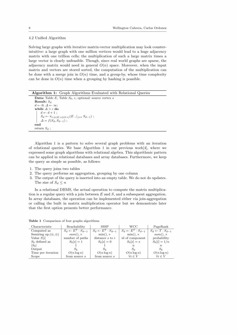
Solving large graphs with iterative matrix-vector multiplication may look counter-intuitive: a large graph with one million vertices would lead to a huge adjacencymatrix with one trillion cells; the multiplication of such a large matrix times alarge vector is clearly unfeasible. Though, since real world graphs are sparse, theadjacency matrix would need in general O(n) space. Moreover, when the inputmatrix and vectors are stored sorted, the computation of the multiplication canbe done with a merge join in O(n) time, and a group-by, whose time complexitycan be done in O(n) time when a grouping by hashing is possible.

Algorithm 1: Graph Algorithms Evaluated with Relational Queries

Data: Table E, Table S0, ε, optional: source vertex sResult: Sdd← 0; ∆←∞;while ∆ > ε do

d← d+ 1 ;Sd ← πi:⊕(E.v⊗S.v)(E ./j=i Sd−1) ;

∆ = f(Sd, Sd−1) ;

endreturn Sd ;

Algorithm 1 is a pattern to solve several graph problems with an iterationof relational queries. We base Algorithm 1 in our previous work[4], where weexpressed some graph algorithms with relational algebra. This algorithmic patterncan be applied in relational databases and array databases. Furthermore, we keepthe query as simple as possible, as follows:

1. The query joins two tables2. The query performs an aggregation, grouping by one column3. The output of the query is inserted into an empty table. We do not do updates.

The size of Sd ≤ n

In a relational DBMS, the actual operation to compute the matrix multiplica-tion is a regular query with a join between E and S, and a subsequent aggregation.In array databases, the operation can be implemented either via join-aggregationor calling the built in matrix multiplication operator but we demonstrate laterthat the first option presents better performance.

Table 1 Comparison of four graphs algorithms

Characteristic Reachability SSSP WCC PageRank

Computed as Sd ← ET · Sd−1 Sd ← ET · Sd−1 Sd ← ET · Sd−1 Sd ← T · Sd−1

Semiring op.(⊕,⊗) sum(),× min(),+ min(),× sum(),×Value S[i] number of paths distance s to i id of component probabilityS0 defined as S0[s] = 1 S0[s] = 0 S0[s] = s S0[i] = 1/n|S0| 1 1 n nOutput Sk Sk Sk SkTime per iteration O(n logn) O(n logn) O(n logn) O(n logn)Scope from source s from source s ∀i ∈ V ∀i ∈ V


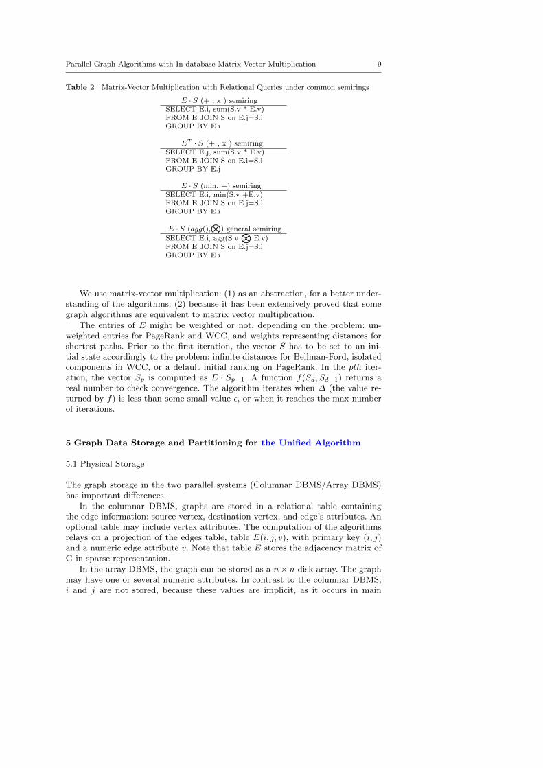
Table 2 Matrix-Vector Multiplication with Relational Queries under common semirings

E · S (+ , x ) semiringSELECT E.i, sum(S.v * E.v)FROM E JOIN S on E.j=S.iGROUP BY E.i

ET · S (+ , x ) semiringSELECT E.j, sum(S.v * E.v)FROM E JOIN S on E.i=S.iGROUP BY E.j

E · S (min, +) semiringSELECT E.i, min(S.v +E.v)FROM E JOIN S on E.j=S.iGROUP BY E.i

E · S (agg(),⊗

) general semiring

SELECT E.i, agg(S.v⊗

E.v)FROM E JOIN S on E.j=S.iGROUP BY E.i

We use matrix-vector multiplication: (1) as an abstraction, for a better under-standing of the algorithms; (2) because it has been extensively proved that somegraph algorithms are equivalent to matrix vector multiplication.

The entries of E might be weighted or not, depending on the problem: un-weighted entries for PageRank and WCC, and weights representing distances forshortest paths. Prior to the first iteration, the vector S has to be set to an ini-tial state accordingly to the problem: infinite distances for Bellman-Ford, isolatedcomponents in WCC, or a default initial ranking on PageRank. In the pth iter-ation, the vector Sp is computed as E · Sp−1. A function f(Sd, Sd−1) returns areal number to check convergence. The algorithm iterates when ∆ (the value re-turned by f) is less than some small value ε, or when it reaches the max numberof iterations.

5 Graph Data Storage and Partitioning for the Unified Algorithm

5.1 Physical Storage

The graph storage in the two parallel systems (Columnar DBMS/Array DBMS)has important differences.

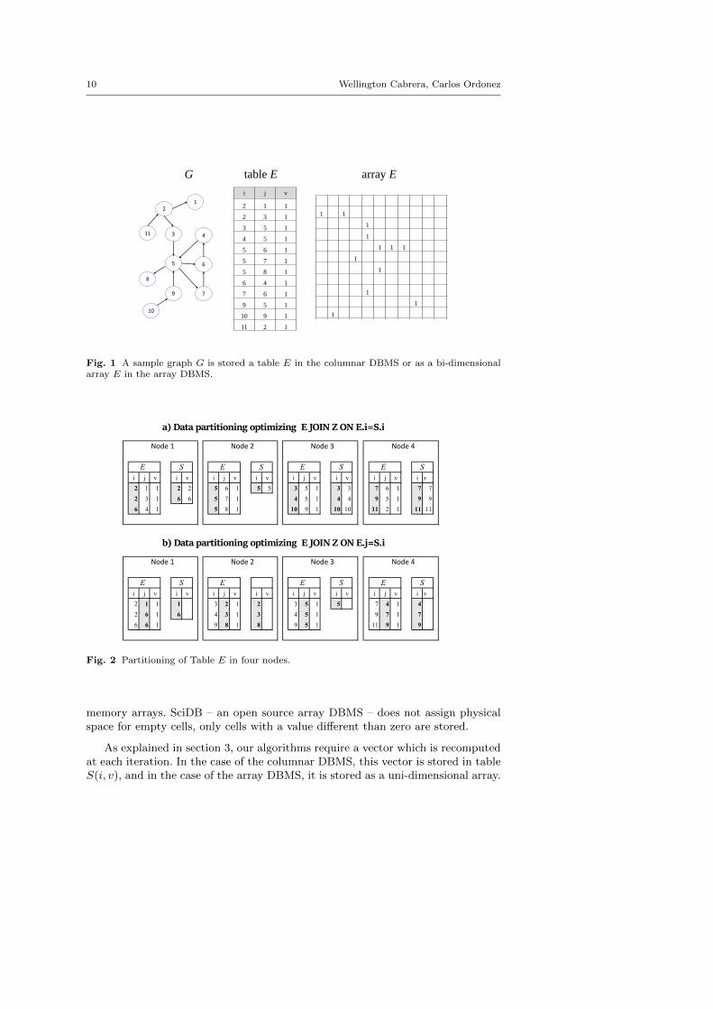
In the columnar DBMS, graphs are stored in a relational table containingthe edge information: source vertex, destination vertex, and edge’s attributes. Anoptional table may include vertex attributes. The computation of the algorithmsrelays on a projection of the edges table, table E(i, j, v), with primary key (i, j)and a numeric edge attribute v. Note that table E stores the adjacency matrix ofG in sparse representation.

In the array DBMS, the graph can be stored as a n× n disk array. The graphmay have one or several numeric attributes. In contrast to the columnar DBMS,i and j are not stored, because these values are implicit, as it occurs in main


21

311

5

4

6

79

8

10

i j v

2 1 1

2 3 1

3 5 1

4 5 1

5 6 1

5 7 1

5 8 1

6 4 1

7 6 1

9 5 1

10 9 1

11 2 1

G table E

1 1

1

1

1 1 1

1

1

1

1

1

array E

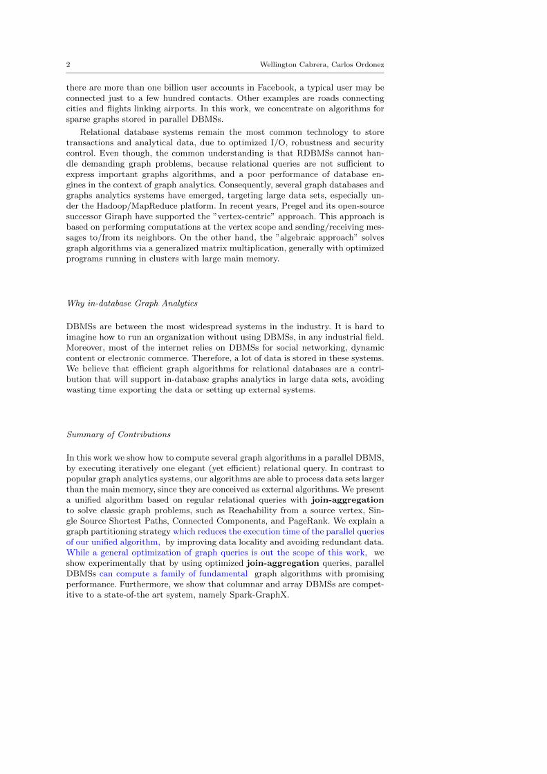
Fig. 1 A sample graph G is stored a table E in the columnar DBMS or as a bi-dimensionalarray E in the array DBMS.

a) Data partitioning optimizing E JOIN Z ON E.i=S.i

Node 1 Node 2 Node 3 Node 4

E E E Ei j v i v i j v i v i j v i v i j v i v

2 1 1 2 2 5 6 1 5 5 3 5 1 3 3 7 6 1 7 7

2 3 1 6 6 5 7 1 4 5 1 4 4 9 5 1 9 9

6 4 1 5 8 1 10 9 1 10 10 11 2 1 11 11

b) Data partitioning optimizing E JOIN Z ON E.j=S.i

Node 1 Node 2 Node 3 Node 4

E E E Ei j v i v i j v i v i j v i v i j v i v

2 1 1 1 3 2 1 2 3 5 1 5 7 4 1 4

2 6 1 6 4 3 1 3 4 5 1 9 7 1 7

6 6 1 9 8 1 8 9 5 1 11 9 1 9

S S S

S S S S

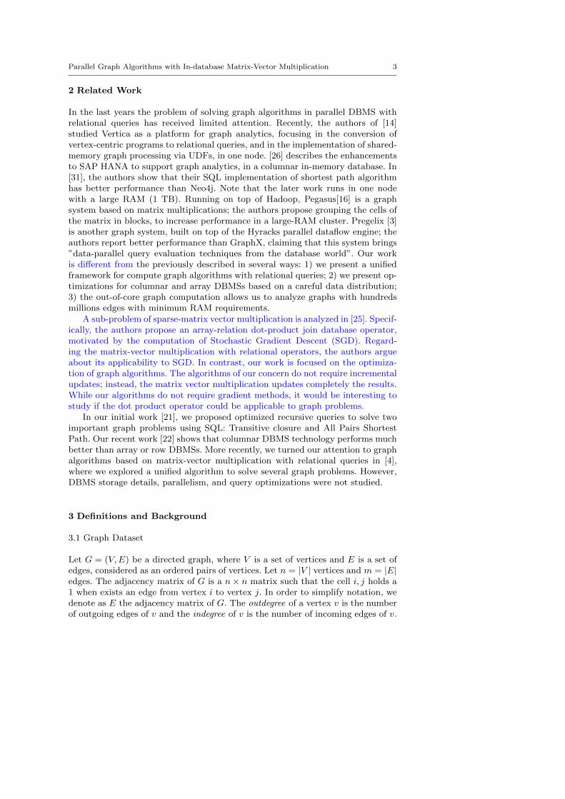
Fig. 2 Partitioning of Table E in four nodes.

memory arrays. SciDB – an open source array DBMS – does not assign physicalspace for empty cells, only cells with a value different than zero are stored.

As explained in section 3, our algorithms require a vector which is recomputedat each iteration. In the case of the columnar DBMS, this vector is stored in tableS(i, v), and in the case of the array DBMS, it is stored as a uni-dimensional array.


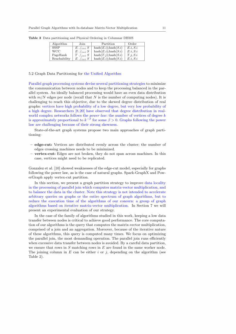
Table 3 Data partitioning and Physical Ordering in Columnar DBMS

Algorithm Join Partition OrderSSSP E ./i=i S hash(E.i);hash(S.i) E.i, S.iWCC E ./i=i S hash(E.i);hash(S.i) E.i, S.iPageRank T ./j=i S hash(T.j);hash(S.i) T.j, S.iReachability E ./i=i S hash(E.i);hash(S.i) E.i, S.i

5.2 Graph Data Partitioning for the Unified Algorithm

Parallel graph processing systems devise several partitioning strategies to minimizethe communication between nodes and to keep the processing balanced in the par-allel system. An ideally balanced processing would have an even data distributionwith m/N edges per node (recall that N is the number of computing nodes). It ischallenging to reach this objective, due to the skewed degree distribution of realgraphs: vertices have high probability of a low degree, but very low probability ofa high degree. Researchers [8,20] have observed that degree distribution in real-world complex networks follows the power law : the number of vertices of degree kis approximately proportional to k−β for some β > 0. Graphs following the powerlaw are challenging because of their strong skewness.

State-of-the-art graph systems propose two main approaches of graph parti-tioning:

– edge-cut: Vertices are distributed evenly across the cluster; the number ofedges crossing machines needs to be minimized.

– vertex-cut: Edges are not broken, they do not span across machines. In thiscase, vertices might need to be replicated.

Gonzalez et al. [10] showed weaknesses of the edge-cut model, especially for graphsfollowing the power law, as is the case of natural graphs. Spark-GraphX and Pow-erGraph apply vertex-cut partition.

In this section, we present a graph partition strategy to improve data localityin the processing of parallel join which computes matrix-vector multiplication, andto balance the data in the cluster. Note this strategy is not intended to acceleratearbitrary queries on graphs or the entire spectrum of graph algorithms, but toreduce the execution time of the algorithms of our concern: a group of graphalgorithms based on iterative matrix-vector multiplication. In Section 7 we willpresent an experimental evaluation of our strategy.

In the case of the family of algorithms studied in this work, keeping a low datatransfer between nodes is critical to achieve good performance. The core computa-tion of our algorithms is the query that computes the matrix-vector multiplication,comprised of a join and an aggregation. Moreover, because of the iterative natureof these algorithms, this query is computed many times. We focus on optimizingthe parallel join, the most demanding operation. The parallel join runs efficientlywhen excessive data transfer between nodes is avoided. By a careful data partition,we ensure that rows in S matching rows in E are found in the same worker node.The joining column in E can be either i or j, depending on the algorithm (seeTable 2).


5.2.1 Partitioning in a Columnar DBMS

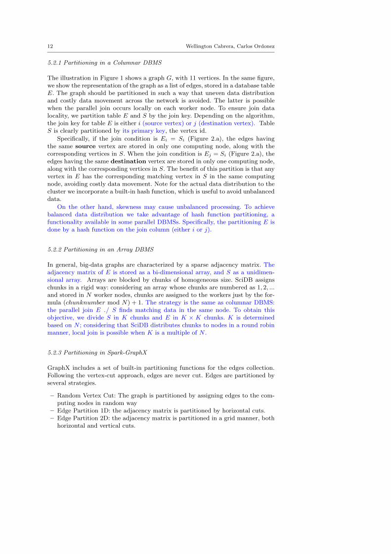
The illustration in Figure 1 shows a graph G, with 11 vertices. In the same figure,we show the representation of the graph as a list of edges, stored in a database tableE. The graph should be partitioned in such a way that uneven data distributionand costly data movement across the network is avoided. The latter is possiblewhen the parallel join occurs locally on each worker node. To ensure join datalocality, we partition table E and S by the join key. Depending on the algorithm,the join key for table E is either i (source vertex) or j (destination vertex). TableS is clearly partitioned by its primary key, the vertex id.

Specifically, if the join condition is Ei = Si (Figure 2.a), the edges havingthe same source vertex are stored in only one computing node, along with thecorresponding vertices in S. When the join condition is Ej = Si (Figure 2.a), theedges having the same destination vertex are stored in only one computing node,along with the corresponding vertices in S. The benefit of this partition is that anyvertex in E has the corresponding matching vertex in S in the same computingnode, avoiding costly data movement. Note for the actual data distribution to thecluster we incorporate a built-in hash function, which is useful to avoid unbalanceddata.

On the other hand, skewness may cause unbalanced processing. To achievebalanced data distribution we take advantage of hash function partitioning, afunctionality available in some parallel DBMSs. Specifically, the partitioning E isdone by a hash function on the join column (either i or j).

5.2.2 Partitioning in an Array DBMS

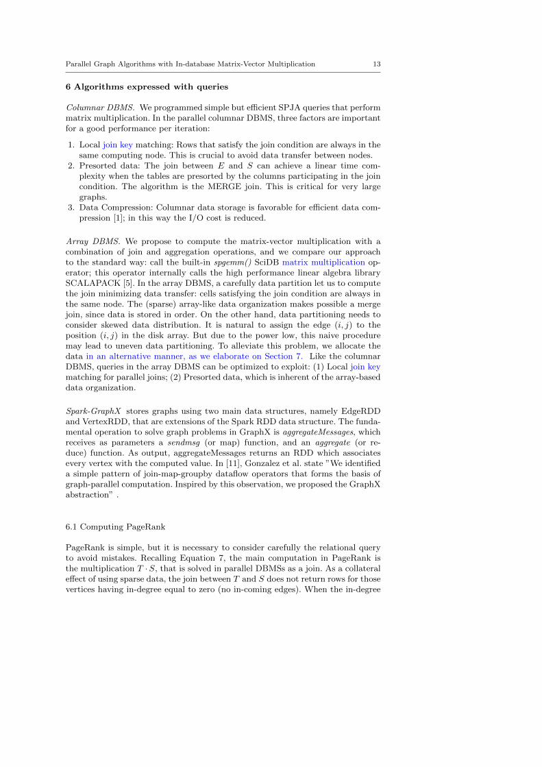
In general, big-data graphs are characterized by a sparse adjacency matrix. Theadjacency matrix of E is stored as a bi-dimensional array, and S as a unidimen-sional array. Arrays are blocked by chunks of homogeneous size. SciDB assignschunks in a rigid way: considering an array whose chunks are numbered as 1, 2, ...and stored in N worker nodes, chunks are assigned to the workers just by the for-mula (chunknumber mod N) + 1. The strategy is the same as columnar DBMS:the parallel join E ./ S finds matching data in the same node. To obtain thisobjective, we divide S in K chunks and E in K × K chunks. K is determinedbased on N ; considering that SciDB distributes chunks to nodes in a round robinmanner, local join is possible when K is a multiple of N .

5.2.3 Partitioning in Spark-GraphX

GraphX includes a set of built-in partitioning functions for the edges collection.Following the vertex-cut approach, edges are never cut. Edges are partitioned byseveral strategies.

– Random Vertex Cut: The graph is partitioned by assigning edges to the com-puting nodes in random way

– Edge Partition 1D: the adjacency matrix is partitioned by horizontal cuts.– Edge Partition 2D: the adjacency matrix is partitioned in a grid manner, both

horizontal and vertical cuts.


6 Algorithms expressed with queries

Columnar DBMS. We programmed simple but efficient SPJA queries that performmatrix multiplication. In the parallel columnar DBMS, three factors are importantfor a good performance per iteration:

1. Local join key matching: Rows that satisfy the join condition are always in thesame computing node. This is crucial to avoid data transfer between nodes.

2. Presorted data: The join between E and S can achieve a linear time com-plexity when the tables are presorted by the columns participating in the joincondition. The algorithm is the MERGE join. This is critical for very largegraphs.

3. Data Compression: Columnar data storage is favorable for efficient data com-pression [1]; in this way the I/O cost is reduced.

Array DBMS. We propose to compute the matrix-vector multiplication with acombination of join and aggregation operations, and we compare our approachto the standard way: call the built-in spgemm() SciDB matrix multiplication op-erator; this operator internally calls the high performance linear algebra librarySCALAPACK [5]. In the array DBMS, a carefully data partition let us to computethe join minimizing data transfer: cells satisfying the join condition are always inthe same node. The (sparse) array-like data organization makes possible a mergejoin, since data is stored in order. On the other hand, data partitioning needs toconsider skewed data distribution. It is natural to assign the edge (i, j) to theposition (i, j) in the disk array. But due to the power low, this naive proceduremay lead to uneven data partitioning. To alleviate this problem, we allocate thedata in an alternative manner, as we elaborate on Section 7. Like the columnarDBMS, queries in the array DBMS can be optimized to exploit: (1) Local join keymatching for parallel joins; (2) Presorted data, which is inherent of the array-baseddata organization.

Spark-GraphX stores graphs using two main data structures, namely EdgeRDDand VertexRDD, that are extensions of the Spark RDD data structure. The funda-mental operation to solve graph problems in GraphX is aggregateMessages, whichreceives as parameters a sendmsg (or map) function, and an aggregate (or re-duce) function. As output, aggregateMessages returns an RDD which associatesevery vertex with the computed value. In [11], Gonzalez et al. state ”We identifieda simple pattern of join-map-groupby dataflow operators that forms the basis ofgraph-parallel computation. Inspired by this observation, we proposed the GraphXabstraction” .

6.1 Computing PageRank

PageRank is simple, but it is necessary to consider carefully the relational queryto avoid mistakes. Recalling Equation 7, the main computation in PageRank isthe multiplication T ·S, that is solved in parallel DBMSs as a join. As a collateraleffect of using sparse data, the join between T and S does not return rows for thosevertices having in-degree equal to zero (no in-coming edges). When the in-degree


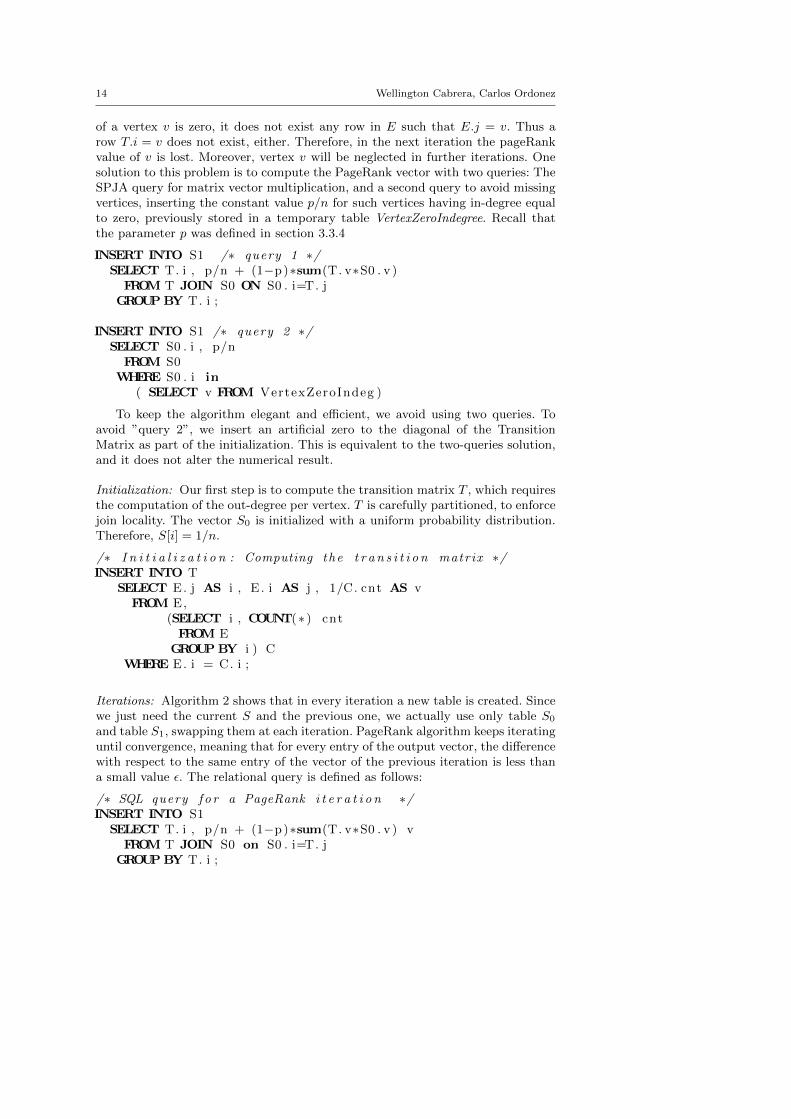
of a vertex v is zero, it does not exist any row in E such that E.j = v. Thus arow T.i = v does not exist, either. Therefore, in the next iteration the pageRankvalue of v is lost. Moreover, vertex v will be neglected in further iterations. Onesolution to this problem is to compute the PageRank vector with two queries: TheSPJA query for matrix vector multiplication, and a second query to avoid missingvertices, inserting the constant value p/n for such vertices having in-degree equalto zero, previously stored in a temporary table VertexZeroIndegree. Recall thatthe parameter p was defined in section 3.3.4

INSERT INTO S1 /∗ query 1 ∗/SELECT T. i , p/n + (1−p)∗sum(T. v∗S0 . v )

FROM T JOIN S0 ON S0 . i=T. jGROUP BY T. i ;

INSERT INTO S1 /∗ query 2 ∗/SELECT S0 . i , p/n

FROM S0WHERE S0 . i in

( SELECT v FROM VertexZeroIndeg )

To keep the algorithm elegant and efficient, we avoid using two queries. Toavoid ”query 2”, we insert an artificial zero to the diagonal of the TransitionMatrix as part of the initialization. This is equivalent to the two-queries solution,and it does not alter the numerical result.

Initialization: Our first step is to compute the transition matrix T , which requiresthe computation of the out-degree per vertex. T is carefully partitioned, to enforcejoin locality. The vector S0 is initialized with a uniform probability distribution.Therefore, S[i] = 1/n.

/∗ I n i t i a l i z a t i o n : Computing the t r a n s i t i o n matrix ∗/INSERT INTO T

SELECT E. j AS i , E . i AS j , 1/C. cnt AS vFROM E,

(SELECT i , COUNT(∗ ) cntFROM E

GROUP BY i ) CWHERE E. i = C. i ;

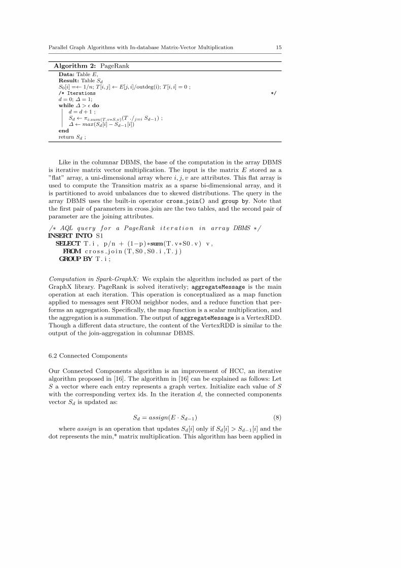
Iterations: Algorithm 2 shows that in every iteration a new table is created. Sincewe just need the current S and the previous one, we actually use only table S0

and table S1, swapping them at each iteration. PageRank algorithm keeps iteratinguntil convergence, meaning that for every entry of the output vector, the differencewith respect to the same entry of the vector of the previous iteration is less thana small value ε. The relational query is defined as follows:

/∗ SQL query f o r a PageRank i t e r a t i o n ∗/INSERT INTO S1

SELECT T. i , p/n + (1−p)∗sum(T. v∗S0 . v ) vFROM T JOIN S0 on S0 . i=T. j

GROUP BY T. i ;


Algorithm 2: PageRank

Data: Table E,Result: Table SdS0[i] =← 1/n; T [i, j]← E[j, i]/outdeg(i); T [i, i] = 0 ;/* Iterations */d = 0; ∆ = 1;while ∆ > ε do

d = d+ 1 ;Sd ← πi:sum(T.v∗S.v)(T ./j=i Sd−1) ;∆← max(Sd[i]− Sd−1[i])

endreturn Sd ;

Like in the columnar DBMS, the base of the computation in the array DBMSis iterative matrix vector multiplication. The input is the matrix E stored as a”flat” array, a uni-dimensional array where i, j, v are attributes. This flat array isused to compute the Transition matrix as a sparse bi-dimensional array, and itis partitioned to avoid unbalances due to skewed distributions. The query in thearray DBMS uses the built-in operator cross join() and group by. Note thatthe first pair of parameters in cross join are the two tables, and the second pair ofparameter are the joining attributes.

/∗ AQL query f o r a PageRank i t e r a t i o n in array DBMS ∗/INSERT INTO S1

SELECT T. i , p/n + (1−p)∗sum(T. v∗S0 . v ) v ,FROM c r o s s j o i n (T, S0 , S0 . i ,T. j )

GROUP BY T. i ;

Computation in Spark-GraphX: We explain the algorithm included as part of theGraphX library. PageRank is solved iteratively; aggregateMessage is the mainoperation at each iteration. This operation is conceptualized as a map functionapplied to messages sent FROM neighbor nodes, and a reduce function that per-forms an aggregation. Specifically, the map function is a scalar multiplication, andthe aggregation is a summation. The output of aggregateMessage is a VertexRDD.Though a different data structure, the content of the VertexRDD is similar to theoutput of the join-aggregation in columnar DBMS.

6.2 Connected Components

Our Connected Components algorithm is an improvement of HCC, an iterativealgorithm proposed in [16]. The algorithm in [16] can be explained as follows: LetS a vector where each entry represents a graph vertex. Initialize each value of Swith the corresponding vertex ids. In the iteration d, the connected componentsvector Sd is updated as:

Sd = assign(E · Sd−1) (8)

where assign is an operation that updates Sd[i] only if Sd[i] > Sd−1[i] and thedot represents the min,* matrix multiplication. This algorithm has been applied in


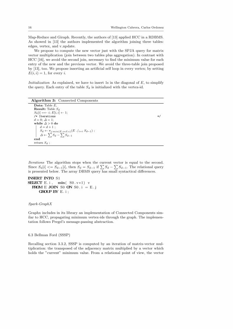
Map-Reduce and Giraph. Recently, the authors of [13] applied HCC in a RDBMS.As showed in [13] the authors implemented the algorithm joining three tables:edges, vertex, and v update.

We propose to compute the new vector just with the SPJA query for matrixvector multiplication (join between two tables plus aggregation). In contrast withHCC [16], we avoid the second join, necessary to find the minimum value for eachentry of the new and the previous vector. We avoid the three-table join proposedby [13], too. We propose inserting an artificial self loop in every vertex; by settingE(i, i) = 1, for every i.

Initialization As explained, we have to insert 1s in the diagonal of E, to simplifythe query. Each entry of the table Sd is initialized with the vertex-id.

Algorithm 3: Connected Components

Data: Table E,Result: Table SdS0[i] =← i; E[i, i]← 1;/* Iterations */d = 0; ∆ = 1;while ∆ > 0 do

d = d+ 1 ;Sd ← πj:min(E.v∗S.v)(E ./i=i Sd−1) ;

∆←∑

Sd −∑

Sd−1

endreturn Sd ;

Iterations The algorithm stops when the current vector is equal to the second.Since Sd[i] <= Sd−1[i], then Sd = Sd−1 if

∑Sd −

∑Sd−1. The relational query

is presented below. The array DBMS query has small syntactical differences.

INSERT INTO S1SELECT E. i , min( S0 . v∗1) v

FROM E JOIN S0 ON S0 . i = E. jGROUP BY E. i ;

Spark-GraphX

Graphx includes in its library an implementation of Connected Components sim-ilar to HCC, propagating minimum vertex-ids through the graph. The implemen-tation follows Pregel’s message-passing abstraction.

6.3 Bellman Ford (SSSP)

Recalling section 3.3.2, SSSP is computed by an iteration of matrix-vector mul-tiplication: the transposed of the adjacency matrix multiplied by a vector whichholds the ”current” minimum value. From a relational point of view, the vector


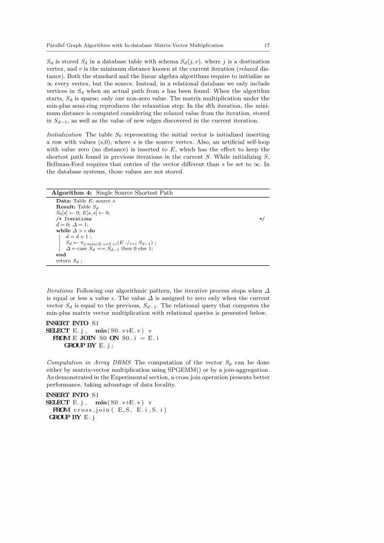
Sd is stored Sd in a database table with schema Sd(j, v), where j is a destinationvertex, and v is the minimum distance known at the current iteration (relaxed dis-tance). Both the standard and the linear algebra algorithms require to initialize as∞ every vertex, but the source. Instead, in a relational database we only includevertices in Sd when an actual path from s has been found. When the algorithmstarts, Sd is sparse; only one non-zero value. The matrix multiplication under themin-plus semi-ring reproduces the relaxation step: In the dth iteration, the mini-mum distance is computed considering the relaxed value from the iteration, storedin Sd−1, as well as the value of new edges discovered in the current iteration.

Initialization The table S0 representing the initial vector is initialized insertinga row with values (s,0), where s is the source vertex. Also, an artificial self-loopwith value zero (no distance) is inserted to E, which has the effect to keep theshortest path found in previous iterations in the current S. While initializing S,Bellman-Ford requires that entries of the vector different than s be set to ∞. Inthe database systems, those values are not stored.

Algorithm 4: Single Source Shortest Path

Data: Table E, source sResult: Table SdS0[s]← 0; E[s, s]← 0;/* Iterations */d = 0; ∆ = 1;while ∆ > ε do

d = d+ 1 ;Sd ← πj:min(E.v∗S.v)(E ./i=i Sd−1) ;∆←case Sd == Sd−1 then 0 else 1;

endreturn Sd ;

Iterations Following our algorithmic pattern, the iterative process stops when ∆is equal or less a value ε. The value ∆ is assigned to zero only when the currentvector Sd is equal to the previous, Sd−1. The relational query that computes themin-plus matrix vector multiplication with relational queries is presented below.

INSERT INTO S1SELECT E. j , min( S0 . v+E. v ) v

FROM E JOIN S0 ON S0 . i = E. iGROUP BY E. j ;

Computation in Array DBMS The computation of the vector Sp can be doneeither by matrix-vector multiplication using SPGEMM() or by a join-aggregation.As demonstrated in the Experimental section, a cross join operation presents betterperformance, taking advantage of data locality.

INSERT INTO S1SELECT E. j , min( S0 . v+E. v ) v

FROM c r o s s j o i n ( E, S , E. i , S . i )GROUP BY E. j


Computation in Spark-GraphX The SSSP routine in the Spark-GraphX library isa standard implementation based on message-passing and aggregation. The fullcode is available in the Spark-GraphX source code repository.

6.4 Reachability from a Source Vertex

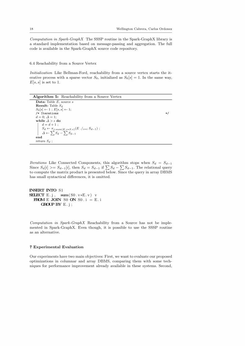
Initialization Like Bellman-Ford, reachability from a source vertex starts the it-erative process with a sparse vector S0, initialized as S0[s] = 1. In the same way,E[s, s] is set to 1.

Algorithm 5: Reachability from a Source Vertex

Data: Table E, source sResult: Table SdS0[s]← 1 ; E[s, s]← 1;/* Iterations */d = 0; ∆ = 1;while ∆ > ε do

d = d+ 1 ;Sd ← πj:sum(E.v∗S.v)(E ./i=i Sd−1) ;

∆←∑

Sd −∑

Sd−1

endreturn Sd ;

Iterations Like Connected Components, this algorithm stops when Sd = Sd−1

Since Sd[i] >= Sd−1[i], then Sd = Sd−1 if∑Sd −

∑Sd−1. The relational query

to compute the matrix product is presented below. Since the query in array DBMShas small syntactical differences, it is omitted.

INSERT INTO S1SELECT E. j , sum( S0 . v∗E. v ) v

FROM E JOIN S0 ON S0 . i = E. iGROUP BY E. j ;

Computation in Spark-GraphX Reachability from a Source has not be imple-mented in Spark-GraphX. Even though, it is possible to use the SSSP routineas an alternative.

7 Experimental Evaluation

Our experiments have two main objectives: First, we want to evaluate our proposedoptimizations in columnar and array DBMS, comparing them with some tech-niques for performance improvement already available in these systems. Second,


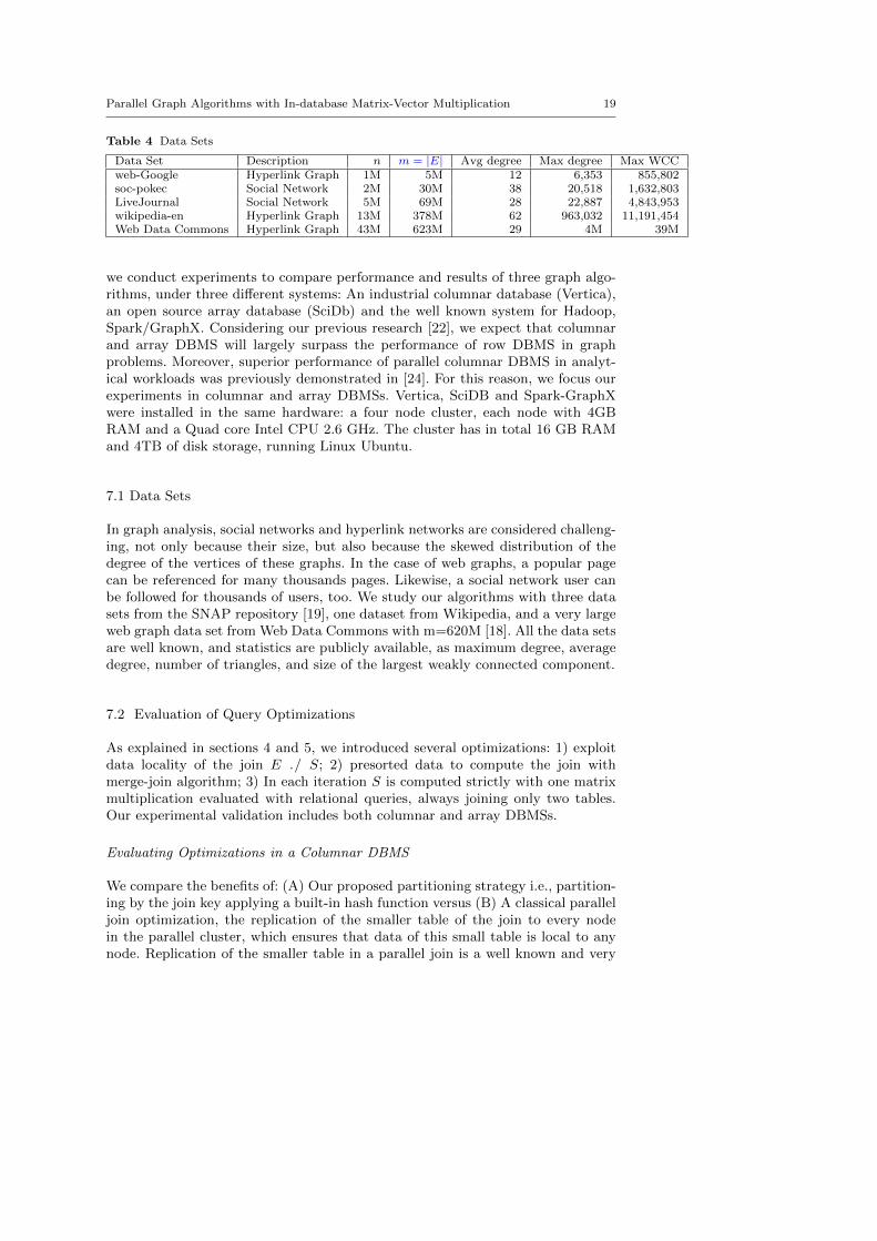
Table 4 Data Sets

Data Set Description n m = |E| Avg degree Max degree Max WCCweb-Google Hyperlink Graph 1M 5M 12 6,353 855,802soc-pokec Social Network 2M 30M 38 20,518 1,632,803LiveJournal Social Network 5M 69M 28 22,887 4,843,953wikipedia-en Hyperlink Graph 13M 378M 62 963,032 11,191,454Web Data Commons Hyperlink Graph 43M 623M 29 4M 39M

we conduct experiments to compare performance and results of three graph algo-rithms, under three different systems: An industrial columnar database (Vertica),an open source array database (SciDb) and the well known system for Hadoop,Spark/GraphX. Considering our previous research [22], we expect that columnarand array DBMS will largely surpass the performance of row DBMS in graphproblems. Moreover, superior performance of parallel columnar DBMS in analyt-ical workloads was previously demonstrated in [24]. For this reason, we focus ourexperiments in columnar and array DBMSs. Vertica, SciDB and Spark-GraphXwere installed in the same hardware: a four node cluster, each node with 4GBRAM and a Quad core Intel CPU 2.6 GHz. The cluster has in total 16 GB RAMand 4TB of disk storage, running Linux Ubuntu.

7.1 Data Sets

In graph analysis, social networks and hyperlink networks are considered challeng-ing, not only because their size, but also because the skewed distribution of thedegree of the vertices of these graphs. In the case of web graphs, a popular pagecan be referenced for many thousands pages. Likewise, a social network user canbe followed for thousands of users, too. We study our algorithms with three datasets from the SNAP repository [19], one dataset from Wikipedia, and a very largeweb graph data set from Web Data Commons with m=620M [18]. All the data setsare well known, and statistics are publicly available, as maximum degree, averagedegree, number of triangles, and size of the largest weakly connected component.

7.2 Evaluation of Query Optimizations

As explained in sections 4 and 5, we introduced several optimizations: 1) exploitdata locality of the join E ./ S; 2) presorted data to compute the join withmerge-join algorithm; 3) In each iteration S is computed strictly with one matrixmultiplication evaluated with relational queries, always joining only two tables.Our experimental validation includes both columnar and array DBMSs.

Evaluating Optimizations in a Columnar DBMS

We compare the benefits of: (A) Our proposed partitioning strategy i.e., partition-ing by the join key applying a built-in hash function versus (B) A classical paralleljoin optimization, the replication of the smaller table of the join to every nodein the parallel cluster, which ensures that data of this small table is local to anynode. Replication of the smaller table in a parallel join is a well known and very


0

200

400

600

800

1000

69 139 208

TIM

E [S

ECO

ND

S]

|E| [MILLIONS OF EDGES]

Execution timeComparing Optimizations - Columnar DBMS

A (proposed) B (classical)

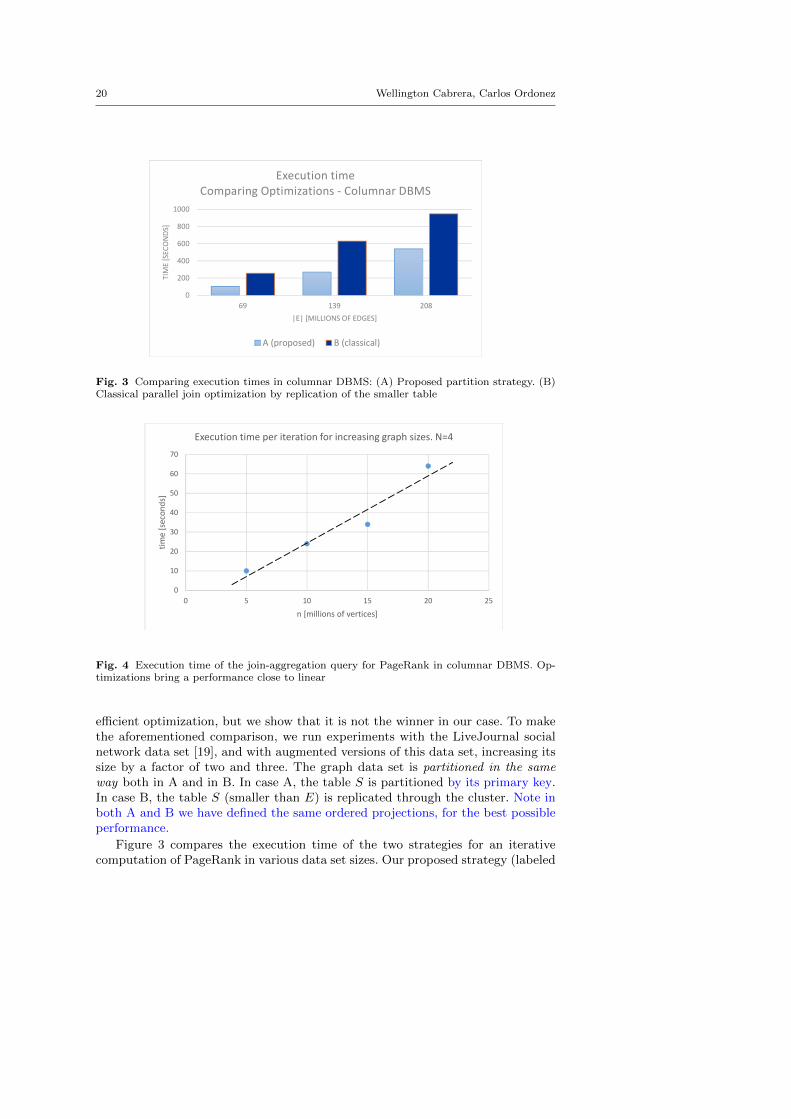
Fig. 3 Comparing execution times in columnar DBMS: (A) Proposed partition strategy. (B)Classical parallel join optimization by replication of the smaller table

0

10

20

30

40

50

60

70

0 5 10 15 20 25

time

[sec

onds

]

n [millions of vertices]

Execution time per iteration for increasing graph sizes. N=4

Fig. 4 Execution time of the join-aggregation query for PageRank in columnar DBMS. Op-timizations bring a performance close to linear

efficient optimization, but we show that it is not the winner in our case. To makethe aforementioned comparison, we run experiments with the LiveJournal socialnetwork data set [19], and with augmented versions of this data set, increasing itssize by a factor of two and three. The graph data set is partitioned in the sameway both in A and in B. In case A, the table S is partitioned by its primary key.In case B, the table S (smaller than E) is replicated through the cluster. Note inboth A and B we have defined the same ordered projections, for the best possibleperformance.

Figure 3 compares the execution time of the two strategies for an iterativecomputation of PageRank in various data set sizes. Our proposed strategy (labeled


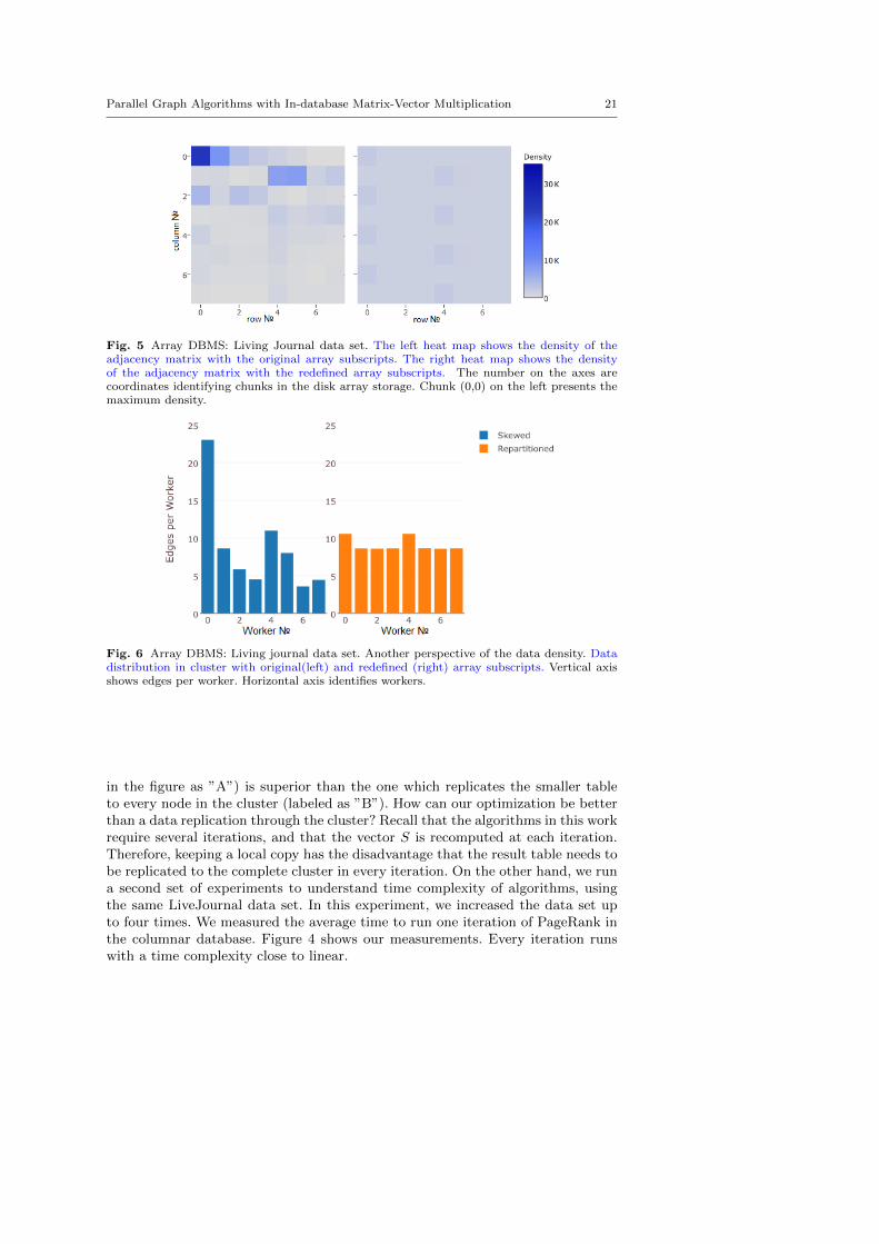
Fig. 5 Array DBMS: Living Journal data set. The left heat map shows the density of theadjacency matrix with the original array subscripts. The right heat map shows the densityof the adjacency matrix with the redefined array subscripts. The number on the axes arecoordinates identifying chunks in the disk array storage. Chunk (0,0) on the left presents themaximum density.

Fig. 6 Array DBMS: Living journal data set. Another perspective of the data density. Datadistribution in cluster with original(left) and redefined (right) array subscripts. Vertical axisshows edges per worker. Horizontal axis identifies workers.

in the figure as ”A”) is superior than the one which replicates the smaller tableto every node in the cluster (labeled as ”B”). How can our optimization be betterthan a data replication through the cluster? Recall that the algorithms in this workrequire several iterations, and that the vector S is recomputed at each iteration.Therefore, keeping a local copy has the disadvantage that the result table needs tobe replicated to the complete cluster in every iteration. On the other hand, we runa second set of experiments to understand time complexity of algorithms, usingthe same LiveJournal data set. In this experiment, we increased the data set upto four times. We measured the average time to run one iteration of PageRank inthe columnar database. Figure 4 shows our measurements. Every iteration runswith a time complexity close to linear.


Evaluating Optimizations in an Array DBMS

In the array DBMS we apply the same strategy as in the columnar DBMS: toincrease the join data locality by partitioning the data properly, as explained inSection 5.2.2. The default way to load the array data may be sensible to skewness,as it is shown on the right side of Figure 5. As a result, a few blocks of the matrixconcentrates a large amount of data. To alleviate the problem of skewed data dis-tribution, we load the array data in an alternative way : redefining array subscriptsof the adjacency matrix. Considering that E is divided in uniform squared-shapedchunks of size h× h, the array subscripts are redefined as follows:

i′ → h ∗ (i mod N) + i/N ; (9)

j′ → h ∗ (j mod N) + j/N ; (10)

Figure 5 shows a plot of the density of the adjacency matrix using originalarray subscripts and redefined array subscripts. Furthermore, Figure 6 shows thedata distribution among the workers. Clearly, the redefinition of array subscriptshelps to alleviate the problem of uneven partitions. To understand if the proposedstrategy has a significant cost, keep in mind that in SciDB an array is loadedin 2 steps: Firstly, data is loaded to a unidimensional array, whose subscript isartificial. Second, the data is partitioned by chunk based on the actual subscripts,an operation known in SciDB as redimensioning. The proposed alternative is toperform the second step (redimensioning) based on redefined indexes instead ofthe original subscripts. The overhead of this alternative, compared to the defaultredimensioning, is just the cost of computing a projection on the original subscripts

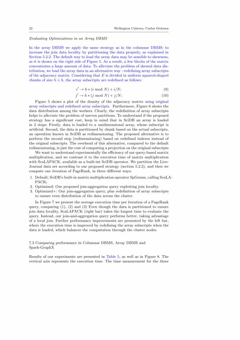
We want to understand experimentally the efficiency of our query-based matrixmultiplication, and we contrast it to the execution time of matrix multiplicationwith ScaLAPACK, available as a built-int SciDB operator. We partition the Live-Journal data set according to our proposed strategy (section 5.2.2), and then wecompute one iteration of PageRank, in three different ways:

1. Default: SciDB’s built-in matrix multiplication operator SpGemm, calling ScaLA-PACK;

2. Optimized: Our proposed join-aggregation query exploiting join locality.3. Optimized+: Our join-aggregation query, plus redefinition of array subscripts

to ensure even distribution of the data across the cluster.

In Figure 7 we present the average execution time per iteration of a PageRankquery, comparing (1), (2) and (3) Even though the data is partitioned to ensurejoin data locality, ScaLAPACK (right bar) takes the longest time to evaluate thequery. Instead, our join-and-aggregation query performs better, taking advantageof a local join. Further performance improvements are presented by the left bar,where the execution time is improved by redefining the array subscripts when thedata is loaded, which balances the computation through the cluster nodes.

7.3 Comparing performance in Columnar DBMS, Array DBMS andSpark-GraphX

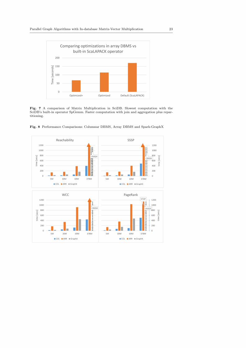
Results of our experiments are presented in Table 5, as well as in Figure 8. Thevertical axis represents the execution time. The time measurement for the three


0

50

100

150

200

Optimized+ Optimized Default (ScaLAPACK)

Tim

e [s

econ

ds]

Comparing optimizations in array DBMS vs built-in ScaLAPACK operator

Fig. 7 A comparison of Matrix Multiplication in SciDB. Slowest computation with theSciDB’s built-in operator SpGemm. Faster computation with join and aggregation plus repar-titioning.

Fig. 8 Performance Comparisons: Columnar DBMS, Array DBMS and Spark-GraphX

CRASH

0

200

400

600

800

1000

1200

5M 30M 69M 378M

time

[sec

s]

SSSP

COL ARR GraphX

CRASH

0

200

400

600

800

1000

1200

5M 30M 69M 378M

time

[sec

s]

WCC

COL ARR GraphX

STOP

CRASH

0

200

400

600

800

1000

1200

5M 30M 69M 378M

time

[sec

s]

PageRank

COL ARR GraphX

CRASH

0

200

400

600

800

1000

1200

5M 30M 69M 378M

time

[sec

s]

Reachability

COL ARR GraphX


Table 5 Comparing Columnar DBMS vs Array DBMS vs Spark-GraphX

Algorithm Data set m = |E| Columnar Array GraphXReachability web-Google 5M 19 141 34

soc-pokec 30M 25 164 59LiveJournal 69M 60 386 166wikipedia-en 378M 364 4311 crashWeb Data Commons 623 2139 stop crash

SSSP web-Google 5M 13 145 34soc-pokec 30M 25 172 59LiveJournal 69M 58 405 166wikipedia-en 378M 487 4574 crashWeb Data Commons 623M 2763 stop crash

WCC web-Google 5M 24 175 32soc-pokec 30M 53 345 83LiveJournal 69M 125 919 451wikipedia-en 378M 443 5091 crashWeb Data Commons 623M 3643 stop crash

PageRank web-Google 5M 18 143 58soc-pokec 30M 72 380 153LiveJournal 69M 99 1073 477wikipedia-en 378M 507 stop crashWeb Data Commons 623M 2764 stop crash

Table 6 Comparison of execution time for exploratory queries under two different data par-titioning methods: by primary key (default) and by joining key (proposed). Times less thanone tenth of second are represented by ◦

Data set mindegree outdegree E.v > c sinks neighbors of vPK JK PK JK PK JK PK JK PK JK

web-Google 5M ◦ ◦ ◦ ◦ ◦ ◦ ◦ ◦ ◦ ◦LiveJournal 69M ◦ ◦ ◦ ◦ 0.2 ◦ ◦ ◦ ◦ ◦wikipedia-en 378M ◦ ◦ ◦ ◦ 3.6 ◦ ◦ ◦ 0.2 ◦

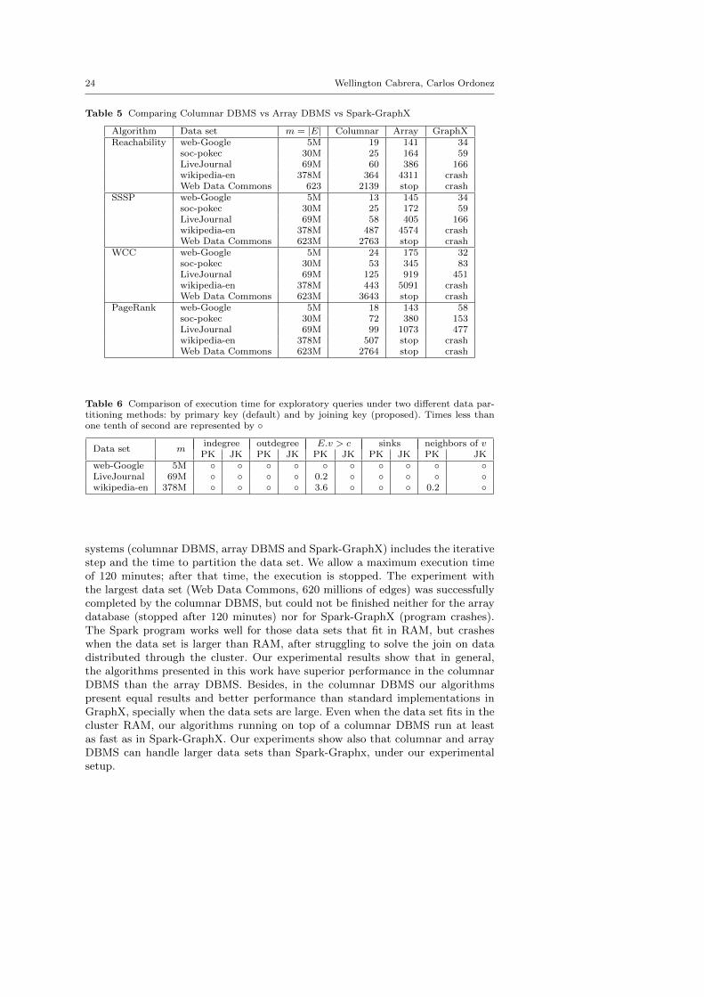
systems (columnar DBMS, array DBMS and Spark-GraphX) includes the iterativestep and the time to partition the data set. We allow a maximum execution timeof 120 minutes; after that time, the execution is stopped. The experiment withthe largest data set (Web Data Commons, 620 millions of edges) was successfullycompleted by the columnar DBMS, but could not be finished neither for the arraydatabase (stopped after 120 minutes) nor for Spark-GraphX (program crashes).The Spark program works well for those data sets that fit in RAM, but crasheswhen the data set is larger than RAM, after struggling to solve the join on datadistributed through the cluster. Our experimental results show that in general,the algorithms presented in this work have superior performance in the columnarDBMS than the array DBMS. Besides, in the columnar DBMS our algorithmspresent equal results and better performance than standard implementations inGraphX, specially when the data sets are large. Even when the data set fits in thecluster RAM, our algorithms running on top of a columnar DBMS run at leastas fast as in Spark-GraphX. Our experiments show also that columnar and arrayDBMS can handle larger data sets than Spark-Graphx, under our experimentalsetup.


0

1

2

3

4

SSSP WCC PageRank

spee

d-up

Parallel speed-up with N=4

web-Google m=5M LiveJournal m=69M wikipedia-en m=380M

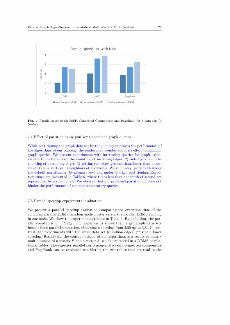
Fig. 9 Parallel speedup for SSSP, Connected Components and PageRank for 3 data sets (4Nodes)

7.4 Effect of partitioning by join key to common graph queries

While partitioning the graph data set by the join key improves the performance ofthe algorithms of our concern, the reader may wonder about its effect to commongraph queries. We present experiments with interesting queries for graph explo-ration: 1) in-degree i.e., the counting of incoming edges; 2) out-degree i.e., thecounting of outcoming edges; 3) getting the edges greater than/lesser than a con-stant; 4) sink vertices 5) neighbors of a vertex v. We run every query both underthe default partitioning (by primary key) and under join key partitioning. Execu-tion times are presented in Table 6, where times less than one tenth of second arerepresented by a small circle. We observe that our proposed partitioning does nothinder the performance of common exploratory queries.

7.5 Parallel speedup experimental evaluation

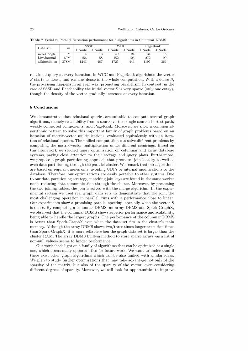
We present a parallel speedup evaluation comparing the execution time of thecolumnar parallel DBMS in a four-node cluster versus the parallel DBMS runningin one node. We show the experimental results in Table 6. By definition, the par-allel speedup is S = t1/tN . Our experiments shows that larger graph data setsbenefit from parallel processing, obtaining a speedup from 2.50 up to 3.8 . In con-trast, the experiments with the small data set (5 million edges) present a lowerspeedup. Recall that the concept behind of our algorithms is a recursive matrixmultiplication of a matrix E and a vector S, which are stored in a DBMS as rela-tional tables. The superior parallel performance of weakly connected componentsand PageRank can be explained considering the two tables that are read in the


Table 7 Serial vs Parallel Execution performance for 3 algorithms in Columnar DBMS

Data set mSSSP WCC PageRank

1 Node 4 Node 1 Node 4 Node 1 Node 4 Nodeweb-Google 5M 14 13 49 24 34 18LiveJournal 69M 156 58 452 125 272 99wikipedia-en 378M 1243 487 1725 443 1195 366

relational query at every iteration. In WCC and PageRank algorithms the vectorS starts as dense, and remains dense in the whole computation. With a dense S,the processing happens in an even way, promoting parallelism. In contrast, in thecase of SSSP and Reachability the initial vector S is very sparse (only one entry),though the density of the vector gradually increases at every iteration.

8 Conclusions

We demonstrated that relational queries are suitable to compute several graphalgorithms, namely reachability from a source vertex, single source shortest path,weakly connected components, and PageRank. Moreover, we show a common al-gorithmic pattern to solve this important family of graph problems based on aniteration of matrix-vector multiplications, evaluated equivalently with an itera-tion of relational queries. The unified computation can solve different problems bycomputing the matrix-vector multiplication under different semirings. Based onthis framework we studied query optimization on columnar and array databasesystems, paying close attention to their storage and query plans. Furthermore,we propose a graph partitioning approach that promotes join locality as well aseven data partitioning through the parallel cluster. We remark that our algorithmsare based on regular queries only, avoiding UDFs or internal modifications to thedatabase. Therefore, our optimizations are easily portable to other systems. Dueto our data partitioning strategy, matching join keys are found in the same workernode, reducing data communication through the cluster. Moreover, by presortingthe two joining tables, the join is solved with the merge algorithm. In the exper-imental section we used real graph data sets to demonstrate that the join, themost challenging operation in parallel, runs with a performance close to linear.Our experiments show a promising parallel speedup, specially when the vector Sis dense. By comparing a columnar DBMS, an array DBMS and Spark-GraphX,we observed that the columnar DBMS shows superior performance and scalability,being able to handle the largest graphs. The performance of the columnar DBMSis better than Spark-GraphX even when the data set fits in the cluster’s mainmemory. Although the array DBMS shows two/three times longer execution timesthan Spark-GraphX, it is more reliable when the graph data set is larger than thecluster RAM. The array DBMS built-in method to store sparse arrays -as a list ofnon-null values- seems to hinder performance.

Our work sheds light on a family of algorithms that can be optimized as a singleone, which opens many opportunities for future work. We want to understand ifthere exist other graph algorithms which can be also unified with similar ideas.We plan to study further optimizations that may take advantage not only of thesparsity of the matrix, but also of the sparsity of the vector, even consideringdifferent degrees of sparsity. Moreover, we will look for opportunities to improve


algorithms beyond graph analytics, exploiting our optimized sparse matrix-vectormultiplication with relational queries.

References

1. D. Abadi, P. Boncz, S. Harizopoulos, S. Idreos, S. Madden, et al. The design and imple-mentation of modern column-oriented database systems. Foundations and Trends R© inDatabases, 5(3):197–280, 2013.

2. Z. Bai, J. Demmel, J. Dongarra, A. Ruhe, and H. van der Vorst. Templates for the solutionof algebraic eigenvalue problems: a practical guide, volume 11. Siam, 2000.

3. Y. Bu, V. Borkar, J. Jia, M. J. Carey, and T. Condie. Pregelix: Big(ger) graph analyticson a dataflow engine. Proc. VLDB Endow., 8(2):161–172, Oct. 2014.

4. W. Cabrera and C. Ordonez. Unified algorithm to solve several graph problems withrelational queries. In Proceedings of the 10th Alberto Mendelzon International Workshopon Foundations of Data Management, Panama City, Panama, May 8-10, 2016, 2016.

5. J. Choi, J. Demmel, I. Dhillon, J. Dongarra, S. Ostrouchov, A. Petitet, K. Stanley,D. Walker, and R. Whaley. Scalapack: a portable linear algebra library for distributedmemory computers–design issues and performance. Computer Physics Communications,97(1-2):1–15, 1996.

6. T. H. Cormen, C. E. Leiserson, R. L. Rivest, and C. Stein. Introduction to Algorithms,Third Edition. The MIT Press, 3rd edition, 2009.

7. D. DeWitt and J. Gray. Parallel database systems: the future of high performance databasesystems. Communications of the ACM, 35(6):85–98, 1992.

8. M. Faloutsos, P. Faloutsos, and C. Faloutsos. On power-law relationships of the internettopology. In ACM SIGCOMM computer communication review, volume 29, pages 251–262. ACM, 1999.

9. J. T. Fineman and E. Robinson. 5. Fundamental Graph Algorithms, chapter 5, pages45–58.

10. J. E. Gonzalez, Y. Low, H. Gu, D. Bickson, and C. Guestrin. Powergraph: Distributedgraph-parallel computation on natural graphs. In Proceedings of the 10th USENIX Confer-ence on Operating Systems Design and Implementation, OSDI’12, pages 17–30, Berkeley,CA, USA, 2012. USENIX Association.

11. J. E. Gonzalez, R. S. Xin, A. Dave, D. Crankshaw, M. J. Franklin, and I. Stoica. Graphx:Graph processing in a distributed dataflow framework. In 11th USENIX Symposium onOperating Systems Design and Implementation (OSDI 14), pages 599–613, 2014.

12. S. Idreos, F. Groffen, N. Nes, S. Manegold, K. Mullender, and M. Kersten. MonetDB:Two decades of research in column-oriented database architectures. IEEE Data Eng.Bull., 35(1):40–45, 2012.

13. A. Jindal, S. Madden, M. Castellanos, and M. Hsu. Graph analytics using vertica relationaldatabase. In Big Data (Big Data), 2015 IEEE International Conference on, pages 1191–1200. IEEE, 2015.

14. A. Jindal, P. Rawlani, E. Wu, S. Madden, A. Deshpande, and M. Stonebraker. Vertex-ica: your relational friend for graph analytics! Proceedings of the VLDB Endowment,7(13):1669–1672, 2014.

15. S. D. Kamvar, T. H. Haveliwala, C. D. Manning, and G. H. Golub. Extrapolation methodsfor accelerating pagerank computations. In Proceedings of the 12th Int. Conf. on WorldWide Web, pages 261–270. ACM, 2003.

16. U. Kang, C. E. Tsourakakis, and C. Faloutsos. Pegasus: A peta-scale graph mining systemimplementation and observations. In Proceedings of the 2009 Ninth IEEE InternationalConference on Data Mining, ICDM ’09, pages 229–238, Washington, DC, USA, 2009.IEEE Computer Society.

17. J. Kepner and J. Gilbert. Graph algorithms in the language of linear algebra, 2011.18. O. Lehmberg, R. Meusel, and C. Bizer. Graph structure in the web: Aggregated by pay-

level domain. In Proceedings of the 2014 ACM Conference on Web Science, WebSci ’14,pages 119–128, New York, NY, USA, 2014. ACM.

19. J. Leskovec and A. Krevl. SNAP Datasets: Stanford large network dataset collection.http://snap.stanford.edu/data, June 2014.

20. A. Mahanti, N. Carlsson, A. Mahanti, M. Arlitt, and C. Williamson. A tale of the tails:Power-laws in internet measurements. IEEE Network, 27(1):59–64, 2013.


21. C. Ordonez. Optimization of linear recursive queries in SQL. IEEE Transactions onKnowledge and Data Engineering (TKDE), 22(2):264–277, 2010.

22. C. Ordonez, W. Cabrera, and A. Gurram. Comparing columnar, row and array DBMSsto process recursive queries on graphs. Information Systems, pages –, 2016.

23. L. Page, S. Brin, R. Motwani, and T. Winograd. The pagerank citation ranking: bringingorder to the web. 1999.

24. A. Pavlo, E. Paulson, A. Rasin, D. Abadi, D. DeWitt, S. Madden, and M. Stonebraker.A comparison of approaches to large-scale data analysis. In Proc. ACM SIGMOD Con-ference, pages 165–178, 2009.

25. C. Qin and F. Rusu. Dot-product join: An array-relation join operator for big modelanalytics. CoRR, abs/1602.08845, 2016.

26. M. Rudolf, M. Paradies, C. Bornhovd, and W. Lehner. Synopsys: large graph analyticsin the SAP HANA database through summarization. In First International Workshop onGraph Data Management Experiences and Systems, page 16. ACM, 2013.

27. F. Rusu and Y. Cheng. A survey on array storage, query languages, and systems. CoRR,abs/1302.0103, 2013.

28. E. Soroush, M. Balazinska, and D. Wang. ArrayStore: A storage manager for complexparallel array processing. In Proc. ACM SIGMOD Conference, pages 253–264, 2011.

29. M. Stonebraker, D. Abadi, A. Batkin, X. Chen, M. Cherniack, M. Ferreira, E. Lau, A. Lin,S. Madden, E. O’Neil, P. O’Neil, A. Rasin, N. Tran, and S. Zdonik. C-Store: A column-oriented DBMS. In Proc. VLDB Conference, pages 553–564, 2005.

30. M. Stonebraker, P. Brown, A. Poliakov, and S. Raman. The architecture of SciDB. InProceedings of SSDBM, SSDBM’11, pages 1–16. Springer-Verlag, 2011.

31. A. Welc, R. Raman, Z. Wu, S. Hong, H. Chafi, and J. Banerjee. Graph analysis: do wehave to reinvent the wheel? In First International Workshop on Graph Data ManagementExperiences and Systems, page 7. ACM, 2013.

32. M. Zaharia, M. Chowdhury, M. J. Franklin, S. Shenker, and I. Stoica. Spark: Clustercomputing with working sets. HotCloud, 10(10-10):95, 2010.

Documents

Scalable Parallel Graph Algorithms with Matrix-Vector ...ordonez/pdf/j-mat-vec.pdf · works and hyper-link real data sets, we present performance comparisons between a columnar DBMS,