Embed Size (px)
Citation preview

Scalable Computing:Practice and Experience
Scientific International Journalfor Parallel and Distributed Computing
ISSN: 1895-1767
⑦⑦⑦⑦
⑦⑦
t
Volume 16(4) December 2015

Editor-in-Chief
Dana Petcu
Computer Science Department
West University of Timisoara
and Institute e-Austria Timisoara
B-dul Vasile Parvan 4, 300223
Timisoara, Romania
Managinig and
TEXnical Editor
Marc Eduard Frıncu
Computer Science Department
West University of Timisoara
and Institute e-Austria Timisoara
B-dul Vasile Parvan 4, 300223
Timisoara, Romania
Book Review Editor
Shahram Rahimi
Department of Computer Science
Southern Illinois University
Mailcode 4511, Carbondale
Illinois 62901-4511
Software Review Editor
Hong Shen
School of Computer Science
The University of Adelaide
Adelaide, SA 5005
Australia
Domenico Talia
DEIS
University of Calabria
Via P. Bucci 41c
87036 Rende, Italy
Editorial Board
Peter Arbenz, Swiss Federal Institute of Technology, Zurich,
Dorothy Bollman, University of Puerto Rico,
Luigi Brugnano, Universita di Firenze,
Giacomo Cabri, University of Modena and Reggio Emilia,
Bogdan Czejdo, Fayetteville State University,
Frederic Desprez, LIP ENS Lyon, [email protected]
Yakov Fet, Novosibirsk Computing Center, [email protected]
Giancarlo Fortino, University of Calabria,
Andrzej Goscinski, Deakin University, [email protected]
Frederic Loulergue, Orleans University,
Thomas Ludwig, German Climate Computing Center and Uni-
versity of Hamburg, [email protected]
Svetozar D. Margenov, Institute for Parallel Processing and
Bulgarian Academy of Science, [email protected]
Viorel Negru, West University of Timisoara,
Moussa Ouedraogo, CRP Henri Tudor Luxembourg,
Marcin Paprzycki, Systems Research Institute of the Polish
Academy of Sciences, [email protected]
Roman Trobec, Jozef Stefan Institute, [email protected]
Marian Vajtersic, University of Salzburg,
Lonnie R. Welch, Ohio University, [email protected]
Janusz Zalewski, Florida Gulf Coast University,
SUBSCRIPTION INFORMATION: please visit http://www.scpe.org

Scalable Computing: Practice and Experience
Volume 16, Number 4, December 2015
TABLE OF CONTENTS
Special Issue on Principles and Practices in Multi-Agent Systems:
Introduction to the Special Issue iii
Combining PosoMAS Method Content with Scrum: Agile Software
Engineering for Open Self-Organising Systems 333
Jan-Philipp Steghofer, Hella Seebach, Benedikt Eberhardinger, Michael
Hubschmann and Wolfgang Reif
Modelling Dynamic Normative Understanding in Agent Societies 355
Christopher Konstantin Frantz, Martin K. Purvis, Bastin Tony Roy
Savarimuthu and Mariusz Nowostawski
A Multi-Agent Approach for Trust-based Service Discovery and
Selection in Social Networks 381
Amine Louati, Joyce El Haddad and Suzanne Pinson
Multi-Objective Distributed Constraint Optimization using Semi-Rings 403
Graham Billiau, Chee Fon Chang and Aditya Ghose
Regular Papers:
Scaling Beyond One Rack and Sizing of Hadoop Platform 423
Wies lawa Litke and Marcin Budka
Energy Efficiency of Parallel Multicore Programs 437
Davor Davidovic, Matjaz Depolli, Tomislav Lipic, Karolj Skala and
Roman Trobec
An Energy-Aware Algorithm for Large Scale Foraging Systems 449
Ouarda Zedadra, Hamid Seridi, Nicolas Jouandeau and Giancarlo Fortino
Overview Papers:
On Processing Extreme Data 467
Dana Petcu, Gabriel Iuhasz, Daniel Pop, Domenico Talia, Jesus
Carretero, Radu Prodan, Thomas Fahringer, Ivan Grasso, Ramon Doallo,
Marıa J. Martın, Basilio B. Fraguela, Roman Trobec, Matjaz Depolli,
Francisco Almeida Rodriguez, Francisco de Sande, Georges Da Costa,
Jean-Marc Pierson, Stergios Anastasiadis, Aristides Bartzokas, Christos
Lolis, Pedro Goncalves, Fabrice Brito, Nick Brown
c⃝ SCPE, Timisoara 2015


Scalable Computing: Practice and Experience
Volume 16, Number 4, pp. iii–iv. http://www.scpe.org
DOI 10.12694/scpe.v16i4.1126ISSN 1895-1767c⃝ 2015 SCPE
INTRODUCTION TO THE SPECIAL ISSUE ON PRINCIPLES AND PRACTICES IN
MULTI-AGENT SYSTEMS
Agent-based Computing addresses the challenges in managing distributed computing systems and networksthrough monitoring, communication, consensus-based decision-making and coordinated actuation. As a result,intelligent agents and multi-agent systems have demonstrated the capability to use intelligence, knowledgerepresentation and reasoning, and other social metaphors like ’trust’, ’game’ and ’institution’, to not only addressreal-world problems in a human-like way but to transcend human performance. This has had a transformativeimpact on many application domains, particularly e-commerce, but also on planning, logistics, manufacturing,robotics, decision support, transportation, entertainment, emergency relief & disaster management, and datamining & analytics. As one of the largest and still growing research fields of Computer Science, agent-basedcomputing today remains a unique enabler of inter-, multi- and trans-disciplinary research.
This special issue provides a selection of papers concerning the state-of-the-art research in multi-agentsystems. Although the idea was initiated at 17th International Conference on Principles and Practice of Multi-Agent Systems, an open call allowed any researcher working on related topics to submit a paper for review.
This special issue features four articles:• The article entitled ”Combining PosoMAS Method Content with Scrum: Agile Software Engineeringfor Open Self-Organising Systems” by Jan-Philipp Steghofer, Hella Seebach, Benedikt Eberhardinger,Michael Hubschmann, Wolfgang Reif proposes PosoMAS-Scrum, an agile agent-oriented software engi-neering process for developing large-scale open self-organising systems. The authors also demonstratehow this method can be applied in a development effort and compare it with existing approaches.
• The article entitled ”Modelling Dynamic Normative Understanding in Agent Societies” by ChristopherKonstantin Frantz, Martin K. Purvis, Bastin Tony Roy Savarimuthu, Mariusz Nowostawski proposesan approach to build up normative understanding from the bottom up without using any prior knowl-edge. Their approach combines both existing institution representations (the structure) with a normidentification process
• The article entitled ”A Multi-Agent Approach for Trust-based Service Discovery and Selection in SocialNetworks” by Amine Louati, Joyce El Haddad, Suzanne Pinson proposes an approach to use multi-agentsystems to model the service discovery and selection process. The authors present a trust model forsocial networks which supports agents in determining trustworthy service providers and allows agentsto reason about trust in their distributed decision-making process.
• The article entitled ”Multi-Objective Distributed Constraint Optimization using Semi-Rings” by Gra-ham Billiau, Chee Fon Chang and Aditya Ghose proposes an extended Support Based Distributed Op-timization algorithm to support Multi-Objective Distributed Constraint Optimization problem. Theauthors also demonstrate that by building a new DCOP definition using an idempotent semiring tomeasure the cost/utility of a solution, this approach is able to solve multiple objectives without a totalpre-order over the set of solutions.
We would like to thank the editorial board of SCPE for the chance of arranging this special issue, and allthe reviewers for their hard work.
Hoa Khanh Dam, Jeremy Pitt, Guido Governatori, Takayuki Ito, Yang Xu.
iii


Scalable Computing: Practice and Experience
Volume 16, Number 4, pp. 333–354. http://www.scpe.org
DOI 10.12694/scpe.v16i4.1127ISSN 1895-1767c⃝ 2015 SCPE
COMBINING POSOMAS METHOD CONTENT WITH SCRUM: AGILE SOFTWARE
ENGINEERING FOR OPEN SELF-ORGANISING SYSTEMS
JAN-PHILIPP STEGHOFER∗AND HELLA SEEBACH, BENEDIKT EBERHARDINGER, MICHAEL HUBSCHMANN,
WOLFGANG REIF†
Abstract. In this paper we discuss how to combine the method content from PosoMAS, the Process for open, self-organisingMulti-Agent Systems, with the agile iterative-incremental life cycle of Scrum. The result is an agile software engineering methodologytailored to open self-organising systems. We show how the methodology has been applied in a development project and discuss thelessons learned. Finally, we compare the Scrum version of PosoMAS to other agile agent-oriented software engineering methodologiesand address the selection of a suitable process.
Key words: Agent-oriented Software Engineering, Self-Organising Systems, Software Engineering Processes
AMS subject classifications. 68T42, 68N30
1. Challenges of Agent-oriented Software Engineering Processes. The fact that multi-agent sys-tems (MAS) and self-organisation have not yet arrived in the software engineering mainstream is a pity, especiallysince the potential of these technologies with regard to robustness, adaptivity, and scalability has been demon-strated (see, e.g., [22, 27, 28]). There are a number of reasons for this situation, not the least of which is thatdiscussion on these topics takes place mostly in academia and very rarely involves actual software companies.Another reason might be that there is a plethora of approaches, often requiring specialised modelling tools andlanguages, and in general ways of thinking about the systems under construction different from “traditional”software engineering, or depending on a certain runtime infrastructure.
Interestingly, these “traditional” processes make no or very little assumption about which kind of softwareis developed with them. They are agnostic of the framework used, the tool, modelling languages, programmingparadigm, and deployment platform. A process like OpenUP [20] is just as useful in building a game for anAndroid phone than it is for building a scientific application. Arguably, this agnosticism is possible due to thefact that the guidance provided by these processes is on such an abstract level. It also considers the managementof the project much more than the actual technical execution. On the other hand, these processes had a longtime to mature and grow with constant feedback from industry and academia.
Agent-oriented methodologies in general follow a different philosophy: instead of focusing on issues of projectmanagement and providing structure for the different technical activities, they describe the way to a technicalsolution in great detail. They are thus much more specific to the domain and often to a certain architecture,tool, or framework. Of course, this takes a lot of the guesswork out of building a multi-agent system andespecially allows inexperienced developers to come up with a solution that uses the somewhat unique or at leastunusual paradigm for a developer familiar with object-oriented programming.
While this philosophy doubtlessly has its merits, it also prevents using the method content developed inthe different approaches to be interchanged and hinders the tailoring of the processes. If we look at the methodcontent of INGENIAS [18] or ASPECS [10], e.g., we can see that many of the activities are specific to themeta-model used and are not compatible with other processes using no or a different meta-model. This isarguably an impediment to cross-fertilisation and convergence towards common standards in the community.
PosoMAS has adopted a different philosophy. As outlined in our previous paper on the process [40] and inSect. 2, it has been created to respond to a number of requirements, including extensibility and customisability aswell as independence from architectures or tools. By following the example of OpenUP and defining independentpractices, the method content is highly adaptable, amenable to tailoring, and can be re-used in different contexts.We therefore consider PosoMAS to be more of a collection of reusable assets than a process in and of itself.
∗Chalmers Technical University — University of Gothenburg, Software Engineering Division, Gothenburg, Sweden ([email protected])
†Augsburg University, Institute for Software & Systems Engineering, Augsburg, Germany ({firstname.lastname}@informatik.uni-augsburg.de, [email protected])
333

334 J.-P. Steghofer, H. Seebach, B. Eberhardinger, M. Hubschmann and W. Reif
The management aspects of the process are provided by a framework process and lifecycle. In this regard,PosoMAS has similarities to O-MaSE [14] but does not enforce the use of a specific tool for process tailoringand modelling.
At the same time, PosoMAS’ technical practices address the needs of a specific subset of MAS that haveso far been somewhat neglected. If a system has to be open and has to exhibit self-organisation, principledsoftware engineering techniques become even more important. For instance, in such cases, the benevolenceassumption, i.e., the assumption that the individual agents contribute to reaching an overall system goal, canno longer be maintained. The dynamics of self-organisation and the potential negative emergent effects arethus coupled with self-interested, erratic, and even potentially malevolent agents that still have to be integratedin the system. Examples for domains that exhibit such effects are energy management [41] and open gridcomputing [6]. Arguably, some of the practices dealing with the specifics of the system class introduce specificmodelling elements or suggest certain notation— but by no means is the developer forced to adopt thesepractices or to comply to a meta-model for the entire project.
Our previous scientific contributions (refer to, e.g., [41, 43, 17, 42]) have dealt with these issues withoutbeing embedded in a methodology for the principled design of such systems. While conceptual and algorithmicsolutions for such problems are often the focus of research, they are rarely embedded in a methodology for theprincipled design of such systems, a shortcoming that we aim to remedy with the PosoMAS method content.
This paper combines the method content of PosoMAS with the project management practices of Scrumand the Agile System Development life-cycle (SDLC) that embeds Scrum sprints in an iterative framework. Itintroduces the requirements that motivate the development of PosoMAS (Sect. 2), outlines the most importantpractices of PosoMAS (Sect. 3), shows how they are embedded in the life cycle (Sect. 4) and demonstrates theway the resulting process can be applied in the development of a MAS (Sect. 5). We also put our work inthe context of other agent-oriented software engineering approaches and in particular compare the PosoMASmethod content and its application to Scrum with Prometheus [32], ASPECS, and with the Scrum version ofINGENIAS in Sect. 6. Finally, we discuss benefits, limitations, and lessons learned in our development efforts(Sect. 7).
The present work extends our previous paper on PosoMAS [40] in several ways: it offers a guideline ofhow the method content can be combined with different life cycles and project management styles based onsituational method engineering and exemplifies the guideline with Scrum; it provides an example showing howthe process can be applied in practice; and it discusses the similarities and differences with INGENIAS-Scrum,a process that has not been part of the analysis before. Since the format of a research paper is insufficientto describe a comprehensive methodology in full detail, the reader is advised to peruse the detailed processdescription at http://posomas.isse.de. The website also offers the method content for use in the EPF Composerand additional information on the comparison of AOSE processes.
2. Requirements for a Process for Large-Scale Open Self-Organising Systems. There are twomain themes that define the requirements we have identified for the design of PosoMAS: the ability to use themethod as readily as standard object-oriented methodologies and the ability to deal with characteristics of openself-organising systems. The individual requirements listed below address those themes and are the basis forthe solution that has been developed. The first four requirements address the need to create an open, flexible,and extensible process. As discussed in Sect. 1 and 6, other MAS methodologies lack this flexibility at thispoint. The requirements listed here are the result of an analysis of existing agent-oriented software engineeringapproaches and reflections of our own experience with processes and engineering of self-organising system (see,e.g., [38, 43]). While they have guided the development of PosoMAS, we consider them work in progress. Aswe gain more experience and confidence in applying the process, we expect to understand the needs better andconsequently refine these requirements.
R1: Accessibility to “traditional” software engineers. We strive to create a process that incorporateselements of agent-oriented software engineering approaches without alienating software engineers that havepreviously worked with “traditional” systems, such as service-oriented or regular object-oriented systems. Oneof the driving factors for this requirement is to allow designers with a software engineering background to usetools that they know and understand and not overwhelm them with agent-oriented specifics from the beginning.This means, e.g., that the process allows the use of any notation, including standards such as UML, and

Combining PosoMAS Method Content with Scrum: Agile Software Engineering for Open Self-Organising Systems 335
thus standard modelling tools. It also means that the process has to be as adaptable and customisable asmethodologies used for object-oriented software engineering.
R2: Architecture and tool agnostic The internal architecture of the agents (such as BDI) should play aslittle role in the high-level design part of the process as the implementation platform on which the agent systemwill run. Object-oriented methodologies such as OpenUP or the V-Model are defined on a level of abstractionthat enables this agnosticism. The methodology should be applicable regardless of the concrete architectureand implementation platform used to allow applicability to a wide array of scenarios.
R3: Level of detail. The process must contain support for all relevant activities in the design process. Itmust make clear which knowledge it assumes the designer to have and point to additional material that can beused to extend the level of understanding. The methodology must contain sufficient guidance and templatesfor the artefacts that must be created. The methodology should also cover the entire life cycle of a softwareengineering methodology, including deployment of the system.
R4: Extensibility and customisability. The methodology must be extendible and it must be possible tocombine it with different process models and to customise it for specific situations as part of a situationalmethod engineering process. This means that it must be possible to use the method chunks put forward inan agile context (e.g., by using it in a specialised Scrum process as described in this paper) as well as in aheavy-weight context (e.g., using the still pervasive waterfall method), or to embed it in the risk/value lifecycle provided by the OpenUP (as described in [40]). It must also be possible to apply situational methodengineering [21] to the process to come up with a methodology suitable for the project, the team, and theenvironment it will be used in.
The second set of requirements deals more directly with the needs present in open self-organising systemsand address their openness, their scale, and the aspect of self-organisation.
R5: Clear separation of different architecture domains. Especially in open systems, development of theindividual agents might not be in the hand of the system designer. In the example of an autonomous powergrid [41], the agents representing the power plants are not designed by the same people that design theirinteraction in the system and set up the infrastructure. Instead, the system designer has to define interfaces,data models, and interactions so that other development teams know how the agents should behave in thesystem, interact with other agents, and with the system as a whole. Even if the system and the individualagents are implemented by the same company, different teams within the organisation can be responsible forthe implementations.
R6: Special focus on interactions between agents and agent organisations. The dynamics of an openself-organising multi-agent system are defined by the interactions between agents within organisations underuncertainty. The behaviour of the individual agent within an organisation plays an important role for thefitness for purpose of the organisation and of its ability to reach its goal within the system. Organisationsand their structure also play an important role in terms of the scalability of the final system. Different systemstructures of organisations—among them hierarchical ones—must be supported by the design activities as wellas requirements elicitation and analysis.
R7: Top-down design vs. bottom-up functionality. While a systems engineering methodology is necessarilytop-down, starting from overall system goals, self-organisation processes and coordinated processes within multi-agent systems provide this striven for functionality in a bottom-up way [43]. A methodology that is suitablefor self-organising systems must take this change of perspective into account and provide appropriate tools forthe design, test, and implementation of bottom-up processes.
In addition to these requirements, we adopt the principles of standard software engineering methods such asOpenUP, that promote reuse, evolutionary design, shared vision, and others. These principles are documented,e.g., in [25] for the Rational Unified Process, a commercial software engineering methodology that introducedmany of the features that are present in modern processes such as OpenUP.
3. PosoMAS in a Nutshell. The technical practices for PosoMAS, compiled in a practice library, coverthe disciplines requirements, architecture, and development. Testing and deployment are the focus of ongoingwork (see, e.g., [16]) since both disciplines are very important in MAS and have not been dealt with sufficiently

336 J.-P. Steghofer, H. Seebach, B. Eberhardinger, M. Hubschmann and W. Reif
Table 3.1: Simplified description of important process modelling concepts.
Concept Description
Practice A collection of method content that addresses a specific issue or allows to achieve aspecific goal. Used by EPF (and PosoMAS) to structure method content. Practices willbe printed in bold font in the following.
Task Describes a unit of work. A task can create or transform a work product and can beassigned to a certain role. It can contain individual steps that have to be performedas part of carrying out the task. Guidances can be provided, e.g., to give guidelines orchecklists. Tasks can be subsumed in activities. They will be printed in italics in thefollowing.
Activity Groups other elements such as tasks, milestones, or other activities. The order of elementswithin the activity is denoted as the work breakdown structure and is established bydefining predecessors for the elements in the structure. Activities will be printed in bold
italics.Work Product Documents, models, code, or other tangible elements that are produced, consumed, and
modified by tasks. Responsibilities for work products can be assigned to roles.Work Product Slot Define an abstract work product that can be instantiated with a concrete one. Play an
important role in the definition of work products that are exchanged between practices.As an example, requirements can be captured in a number of concrete work products,e.g., in a use-case model, in user stories, or in a systems goal model. Using the moregeneric work product slot [Requirements Model] allows specifying that requirements areused by a practice but does not prescribe which kind of requirements are necessary. Workproduct slots are fulfilled with concrete work products in the assembly of the process. Todifferentiate a work product slot from a work product, the former is always enclosed insquare brackets.
Role Denotes an individual or a group of individuals with a certain set of skills, competencies,and responsibilities required in the process. Different roles can be filled by different peopleduring the process and an individual can fill several roles if required.
Process Defines the sequence of activities and tasks, phases, and milestones to get to the finalproduct. Within a process, concrete roles, tasks, work products, etc. are defined. Atailored process for a specific project is modelled as a Delivery Process. In EPF, partialprocesses are captured in Capability Patterns.
Guidance Provides additional information about the elements in the method content. Differentkinds of guidances are possible: guidelines, templates, checklists, tool mentors, supportingmaterials, reports, concepts, examples, and others.
as of yet. It is possible, however, to use practices from other processes for these issues as illustrated in Sect. 4.2.All PosoMAS method content is specified using SPEM1. The most important SPEM concepts used in thefollowing are detailed in Table 3.1. Furthermore, PosoMAS makes use of EPF2. EPF provides a commonbaseline for process development by providing a usable version of SPEM as well as a tool to define processes,the EPF Composer. In addition, it provides process content in the form of method libraries, such as a modelof OpenUP. The EPF method libraries introduce a number of commonly used concepts, such as pre-definedroles for developers and architects. PosoMAS makes use of these common concepts instead of re-defining them,extends them if necessary and adds many specific elements that are not covered in the standard libraries.
1Software & Systems Process Engineering Metamodel (http://www.omg.org/spec/SPEM/2.0/), defined by the Object Manage-ment Group (OMG).
2Eclipse Process Framework (EPF): http://epf.eclipse.org/

Combining PosoMAS Method Content with Scrum: Agile Software Engineering for Open Self-Organising Systems 337
3.1. Rationale and Structure of PosoMAS. We adopt the notion of situational method engineer-ing [21]: while we define method content (i.e., tasks, activities, work products, guidance, etc.) and in someaspect also the order in which this method content should be applied, the content is formulated in such a waythat a process engineer can use it to construct a specific instance of a process tailored to the development effortat hand. This means that the method content (collected in practices that address specific needs and purposes)is combined with a specific life cycle and selections are made, how the content is used, who is going to fill theroles, and which work products are created and used. The creation of a specific process instance from existingmethod content is known as process tailoring. Allowing this flexibility and adaptability addresses requirementR4: Extensibility and customisability.
The practices that contain the method content in PosoMAS introduce techniques for the principled de-sign of individual agents, organisations, their interactions, as well as the overall system and the environment.The categorisation of these techniques is an important aspect of the design of the process and addresses therequirement for R5: Clear separation of different architecture domains:
Agent Architecture: the design of the individual agents, separate for each type of agent relevant in thesystem.
Agent Organisation: the specification of organisational paradigms that will structure the agent populationat runtime.
Agent Interaction: the definition of interfaces and protocols used by agents to exchange information, delegatecontrol, and change their organisational structure.
System Architecture: the design of the entire system, including the relationship between the different typesof agents, the supporting infrastructure, and external components as well as the environment.
The PosoMAS method content is connected by the use of work product slots to exchange informationbetween the activities and tasks specified for each practice. As an example for exchange within PosoMAS,consider Practice: Agent Environment Design. It contains tasks that describe how a work product slot[Requirements Model] is used as the basis for identification of the necessary infrastructure to support the MASunder construction (e.g., external services that must be used, relevant actors that require an interface to thesystem). The identified infrastructure, which interfaces are necessary, and what these interfaces look like iscaptured in the Multi-Agent System Architecture work product. This work product is used by other practices,such as Practice: Evolutionary Agent Design or Practice: Organisational Design as an input for theirown design decisions. The flow of work products thus defines how the practices and activities within PosoMASare connected.
These work products are also the interface to method content from other processes. INGENIAS, e.g., offersmethod content for the design of BDI agents. If a concrete process instance for a specific project wants tomake use of this method content, it can, e.g., use the activity Generate Agent Model [18] from INGENIAS. Thisactivity creates a concrete instantiation of the work product slot [Agent Architecture], as defined in PosoMAS.Since all practices in PosoMAS are independent of the concrete instantiation of this work product slot, butrather require abstract properties (the instantiation should be a description of the internal architecture of anagent), the content from different processes can be readily combined. In this way, the work product slots actcomparably to interfaces in object-oriented programming.
PosoMAS does not prescribe a specific modelling language or a certain tool chain. Instead, it suggests theuse of UML and gives the developers support in that by providing a corresponding UML profile for the definitionof agent concepts. This addresses R1: Accessibility to “traditional” software engineers and R2: Architectureand tool agnostic.
3.2. Overview of PosoMAS practices. As PosoMAS is targeted at open systems, the architecturaltasks are aimed at providing standardisation, separation of concerns, and interoperability. The applicability toa wide range of target systems has also been a concern. Therefore, even though some content of the practices isspecific to open self-organising MAS, they do not require the use of a specific meta-model or agent architecture,again addressing R2: Architecture and tool agnostic. The concrete practices are also tailored to address R6:Special focus on interactions between agents and agent organisations, a requirement that has greatly influencedthe practice Practice: Organisational Design, and R7: Top-down design vs. bottom-up functionality whichis evident, e.g., in Practice: Goal-driven Requirements Elicitation and the interplay between Practice:

338 J.-P. Steghofer, H. Seebach, B. Eberhardinger, M. Hubschmann and W. Reif
Evolutionary Agent Design and Practice: Organisational Design. The practice library provides thepractices described briefly below. Missing from the content here is Practice: Trust-based Interaction
Design, as it has not been applied in the case study. It encompasses the design and implementation of a trustand reputation system to deal with agents for which the benevolence assumption does not hold. Please notethat rather than stating the concrete outputs of the practices below, we state the work product slots that theoutputs can fill, in order to show how the practices can be combined.
Practice: Goal-driven Requirements Elicitation
Description: Operationalises the technique for requirements elicitation based on KAOS [26] and the work ofCheng et al. [9]. The purpose of this practise is to provide an iterative process to successivelyrefine the goal model until a complete model of the system requirements is gained. Beside thesystem goal model, a conceptual domain model as well as a glossary of the domain are outputsof this practice. The approach is ideally suited for adaptive systems since uncertainties andtheir mitigation can be directly modelled in the requirements. This allows the stakeholders toreason about countermeasures and identify risks early on. The practice is easily embedded initerative-incremental processes. System goals can be elaborated in different iterations, with apreference to elaborate those first that have the greatest potential impact and risk. Guidelinesdetail the application of the practice in an agile environment and how to capture processsupport requirements. We demonstrate in Sect. 5 how this practice can be integrated with thebacklogs used in Scrum.
Main Input: Vision DocumentMain Output: Requirements Model
Practice: Pattern-driven MAS Design
Description: Provides guidance to design a MAS based on existing architectural, behavioural, and inter-action patterns and reference architectures. These three types of patterns correspond to thesystem architecture, agent architecture, and agent interaction areas. The practice enablesreuse, avoids making mistakes twice, and allows tapping into the knowledge that has beencreated elsewhere for a cleaner, leaner, and more flexible design.
Main Input: [Agent Architecture], [Interaction Model], [Multi-Agent System Architecture], [RequirementsModel]
Main Output: [Agent Architecture], [Interaction Model], [Multi-Agent System Architecture], ArchitecturalStyle Notebook
Practice: Evolutionary Agent Design
Description: Describes an approach to design agents and their architecture in an evolutionary way thatenhances the design over time while requirements become clearer and development progresses.During the development process, the agent types, their capabilities and behaviour, their in-ternal architecture, and their interactions become clearer as the requirements mature anddevelopment progresses towards a shippable build. To allow the product to mature this way,the design of the agents has to adapt to new knowledge continuously and become more specificby refinement when necessary and incorporating changes in the requirements or the systemenvironment.
Main Input: [Requirements Model]Main Output: [Agent Architecture], [Interaction Model], [Multi-Agent System Architecture]

Combining PosoMAS Method Content with Scrum: Agile Software Engineering for Open Self-Organising Systems 339
Practice: Agent Environment Design
Description: Outlines how the system the agents are embedded in is designed and how the agents interactwith it. This pertains to the System Architecture aspect. A MAS not only consists of au-tonomous agents but also incorporates a multitude of additional often grounded infrastructure,external actors, interfaces, hardware, and environmental factors. These can have a significantimpact on the overall system design and should be regarded early on. The practice providestasks to identify these factors and incorporate them in the design of the overall system. Thisincludes the identification and design of necessary interfaces between the agents and to externalcomponents in the system’s environment as well as the identification of uncertainty factors inthe environment.
Main Input: [Interaction Model], [Requirements Model]Main Output: [Multi-Agent System Architecture], [System Environment Description], [Interaction Model]
Practice: Organisational Design
Description: Describes the design of the organisation [23] the agents will interact in, thus addressing theAgent Organisation aspect. Multi-agent systems with many interacting agents require a form ofstructure or organisation imposed on the population. Sometimes, this structure is permanent,such as a hierarchy that determines the delegation of control and propagation of information, ortransient, such as a coalition in which agents interact until a certain common goal is reached.The system designer has to decide which organisations are suitable for the system to reachthe stated goals and implement mechanisms that allow the formation of these organisationalstructures at runtime. If this process is driven from within the system, “self-organisation” ispresent.
Main Input: [Multi-Agent System Architecture], [Requirements Model]Main Output: [Agent Organisation Definition]Guidance: Bryan Horling and Victor Lesser – A Survey of Multi-Agent Organizational Paradigms
(Whitepaper) [23]
Practice: Model-driven Observer Synthesis
Description: Describes how observer implementations can be synthesized from constraints specified in therequirements documents as described in [17]. In adaptive systems, it is necessary to observethe system and react if the system enters an undesirable state or shows unwanted behaviour.For this purpose, feedback loops, operationalised as observer/controllers can be employed [36].Therefore, this practice supports the developer on the automatic transformation of specifiedconstraints into observers that monitor these constraints at runtime. A prerequisite of thispractice is that constraints have been captured during requirements analysis. The process canbe repeated after the requirements or the domain model have changed, according to a model-driven design (MDD) approach. Changed parts of the system models and implementation willbe re-generated while existing models and code are preserved.
Main Input: [Agent Architecture], [Interaction Model], [Multi-Agent System Architecture], [RequirementsModel]
Main Output: Observation Model, ImplementationGuidance: How to adopt the Model-driven Observer Synthesis practice (Roadmap), Observation Model
(Concept), Observer/Controller Architecture (Concept), Benedikt Eberhardinger et al. –Model-driven Synthesis of Monitoring Infrastructure for Reliable Adaptive Multi-Agent Sys-tems (Whitepaper) [17]
Each practice is defined by an appropriate guidance in EPF that states the purpose of the practice, givesa description, and provides a brief instruction on how the elements of the practice relate to each other and inwhich order they should be read. The practice usually references a roadmap that describes how a novice shouldapproach adopting this practice, a list of key concepts and white papers, and a set of helpful material in theform of guidances, thus addressing the requirement to have the necessary R3: Level of Detail. A practice also

340 J.-P. Steghofer, H. Seebach, B. Eberhardinger, M. Hubschmann and W. Reif
takes one or several work products (or work product slots) as inputs and outputs.For use within a process, tasks from different practices are combined in activities. These activities are often
addressing a common theme. For PosoMAS-Scrum, e.g., the activity Develop Agent Architecture combines tasksfrom Practice: Pattern-driven MAS Design and Practice: Evolutionary Agent Design. Activities andtasks can in turn be combined in capability patterns (nested activities, so to speak) such as Design ArchitectureComponents. These patterns are then arranged within the lifecycle as demonstrated in Sect. 4.2.
The detailed practice descriptions and the models for use in EPF are available at http://posomas.isse.de.We thus provide a repository for method content and make reusable assets available for combination withmethod content from other processes, fulfilling the appeal of the IEEE FIPA Design Process Documentationand Fragmentation Working Group and many authors (e.g., [39, 11]).
4. The PosoMAS-Scrum Life Cycle. The process life cycle determines the progression of a productunder development in the context of the process, the stakeholders, and the environment. A well-defined lifecycle provides guidance w.r.t. the order of activities the Scrum Team has to perform, the project milestonesand deliverables, and the progress of the product. The advancement of a product development effort can thusbe measured based on the planned and the actual progress within the life cycle. Scrum is an example of alight-weight process framework that embraces the Agile Manifesto [5]. It consists of a number of rules thatprescribe how roles, events, and artefacts have to be combined for a Scrum Team to manage a complex softwaredevelopment project and create value for the customer [37]. Within these boundaries it is possible to applycustom development practices. Scrum has been modelled in the EPF Composer by Mountain Goat Software3
and a method plugin containing the method content is available. The customisation is based on a significantextension of this method content.
4.1. Structure of Scrum. At the core of Scrum is the insight that it is impossible to conclusively definerequirements and that it is therefore necessary to include the client in all phases of the development and be ableto react to changes in the requirements quickly. A change request is thus not an exceptional event but somethingrather normal, making it very easy to incorporate changes into the development process. The decisions of theproject team are always based on what is currently known about the project, a principle called empiricism [37].This makes it necessary to form decisions transparent for the stakeholders, inspect past decisions based on newdata regularly, and adapt if the circumstances have changed.
The other principle is the focus on a self-organising Scrum Team. While different roles still exist, Scrumpromotes the notion that different members of the Scrum Team assume these roles of their own accord. TheScrum Team decides internally how the work is split among the team members and is involved in all importantdecisions, including assessment of the effort required to perform certain tasks. A Scrum Master is designatedin each team who ensures that the Scrum rules are adhered to, but also acts as a spokesperson for the ScrumTeam and coordinates communication with external stakeholders. Importantly, a Product Owner, ideally arepresentative of the client with the authority to make decisions about the product and embedded in the ScrumTeam, defines the requirements and prioritises them by importance. She is also available to the Scrum Team toanswer questions and relay issues that come up during development to the client organisations. The ProductOwner has, however, no authority over the Scrum Team [37].
The most important communication device between the Scrum Team and the Product Owner is the ProductBacklog. It contains all currently known and open requirements for the product, including features and non-functional requirements [37]. While Scrum does not prescribe the form in which requirements are represented inthe product backlog, they are often captured in the form of user stories (see, e.g., [31]). A user story describeswho wants to achieve what and why. Regardless of the form the requirements take, they are ordered in thebacklog according to their risk, customer value, complexity, or any other criteria the Product Owner deemsreasonable.
The Scrum Team estimates the effort required to realise the requirements. As part of a “grooming” process,the Product Owner and the Scrum Team together refine the requirements, re-order them and adapt estimates.As part of a Sprint Planning Meeting, the requirements that will be tackled in the next development iteration—
3The corresponding content can be found in a human-readable form at http://epf.eclipse.org/wikis/scrum/, made availableunder the Eclipse Public License v1.0.

Combining PosoMAS Method Content with Scrum: Agile Software Engineering for Open Self-Organising Systems 341
Potentially Shippable
Product Increment
Sprint
Finalisation
Sprint
Planning
Daily Work
Sprint
2 to 4 Weeks
Daily Scrum
Initial Requirements
Sprint
Backlog
Product
Backlog
Highest Priority
Work Items
Release to
Production
Defect Reports and
Change Requests
Enhancement and Change Requests
Construction Iterations
Working System
Fig. 4.1: Ambler et al.’s Agile System Development life-cycle (SDLC) [3] as used for PosoMAS-Scrum. SDLCis an extension of the standard Scrum sprint life cycle with iterations and consideration of preparatory as wellas release activities. Initial requirements are captured in a Product Backlog. An iteration consists of SprintPlanning, in which the backlog is prioritised and the work items for the sprint are selected. The sprint itselfconsists of small increments of Daily Work, initiated by a Daily Scrum. After the 2 to 4 weeks of the sprintare completed, a Potentially Shippable Product Increment has been created. The Sprint Review, which togetherwith the Sprint Retrospective constitutes the Sprint Finalisation, gives all stakeholders the opportunity forfeedback. After construction is complete, the working system is released to production. The product backlogcan be changed or augmented by the stakeholders at any time during or after a sprint.
called a Sprint —are picked and transferred into the Sprint Backlog. During the sprint, the Scrum Team createsa complete Potentially Shippable Product Increment that realises the picked requirements (the Sprint Goal) overa time horizon of a month. The Product Owner can cancel the sprint if the Sprint Goal no longer aligns withthe client organisation goals.
During a sprint, daily structured meetings are performed to further communicate between the Scrum Teammembers and to assess the progress of the sprint. These Daily Scrums—also called Standup Meetings sincethey are usually held with all participants standing—are 15-minute meetings in which the progress, the plannedwork, and any issues are discussed [37]. In larger projects, a Scrum of Scrums can be used with similar rules tocoordinate between different Scrum Teams. Scrum promotes co-location of all team-members, meaning that it iseasy to communicate directly with other members of the team, to exchange information, and to help each otherwith technical difficulties. When the sprint is concluded, the Scrum Team presents the Potentially ShippableProduct Increment to the Product Owner during the Sprint Review and fulfilment of the Sprint Goal as wellas future requirements and necessary changes are discussed. Finally, the Sprint Retrospective gives the ScrumTeam a chance to reflect on the last sprint and discuss possible improvements.
4.2. Embedding PosoMAS practices in Scrum. The description above does not include concretedevelopment practices. Indeed, Scrum is seen as a framework, defining rules and an environment, in whichconcrete development practices can be applied. Scrum does not per se include a process life-cycle in whichthe method content can be embedded. It introduces the notion of a sprint but there are no defined places forthe preparatory and release work. Therefore, we use a variant of the “Agile System Development life-cycle(SDLC)” [3], that embeds the elements Scrum provides. It contains a framework for the individual sprints,including project setup and initial requirements and deployment and operation. Sprints are embedded initerations which contain sprint planning and review. The version of the life-cycle used here is shown in Fig. 4.1.
The PosoMAS practices are used within a sprint embedded within an iteration of the SDLC. An iteration,depicted in Fig. 4.2 embeds the activities defined in the PosoMAS practices library in a Scrum sprint. TheScrum Team decides which activities, sub-activities and tasks it has to tackle each given day. This gives thema flexible structure within which to work. All guidances, work products, and other method content defined inthe PosoMAS practices are at their disposal. In general, Scrum puts less focus on documentation. Therefore,

342 J.-P. Steghofer, H. Seebach, B. Eberhardinger, M. Hubschmann and W. Reif
Sprint Planning Sprint Sprint Finalisation
Estimate theproduct backlog
Prioritizing theproduct backlog
Estimate Velocity
Sprint PlanningMeeting
Task Breakdown
Sprint ReviewMeeting
SprintRetrospective
Daily Scrum
ClarifyRequirements
Update theproduct backlog
Define AgentOrganisations
Design ArchitectureComponents
Design SystemDynamics
DevelopSolution Increment
Develop Trust-Based Interactions
Specify AgentInteractions
Prepare PotentiallyShippable Build
Prepare SprintReview
Fig. 4.2: Structure of an iteration in PosoMAS-Scrum, combining method content from PosoMAS, Scrum, andOpenUP. An iteration is started by preparatory activities to produce a new version of the product backlog andselect requirements for the sprint. During the sprint, the activities from PosoMAS (highlighted) are performedas required during the daily work. The sprint ends after a certain time or when all backlog items have beentackled with a Sprint Review and a Sprint Retrospective.
a Scrum Team can decide to create less models or combine models suggested by PosoMAS activities andtasks. Since most of the management documents have been defined in the OpenUP and are not present in thePosoMAS-Scrum method configuration, no additional customisation has to be performed in this regard.
PosoMAS adds most of its method content in the design activities and replaces use cases with systemgoals as the main model to capture requirements. Therefore, PosoMAS-Scrum has requirements engineeringactivities in parallel to the ongoing development work, performed mostly by the Product Owner. The ScrumTeam estimates requirements whenever necessary. The sprint backlog that contains those requirements thatwill be tackled in a sprint is created from the Product Backlog during the Sprint Planning Meeting. Initialrequirements are captured in the release planning stage, before the sprints are begun, a task similar to the InitiateProject activity described for the OpenUP earlier [40]. The product backlog is refined by new requirementsthat are created during sprints or come up during the Sprint Review. PosoMAS-Scrum does not prescribethe way requirements are captured and the example in the next section shows how goal-oriented requirementsengineering can be used in this context. This is an example of process tailoring where the generic process hasbeen adapted to suit the needs of the development effort.
PosoMAS-Scrum also encompasses activities to prepare the release of the product. For this purpose, methodcontent from the OpenUP practice Production Release has been embedded at the end of the life cycle to provideguidance for the eventual rollout of the finished product. The use of this practice from a different process alsoillustrates the modularity of PosoMAS and OpenUP and how their elements can be combined beneficially.
5. Sprint Example. We present how PosoMAS-Scrum is applied in a case study that shows an excerpt ofthe development of a highly dynamic, self-organising material handling and order fulfilment system constitutinga self-organising warehouse system inspired by the Kiva System [24]. The system has been developed in collab-

Combining PosoMAS Method Content with Scrum: Agile Software Engineering for Open Self-Organising Systems 343
oration with students applying PosoMAS-Scrum and now serves as a proving ground for new self-optimisationand self-adaptation mechanisms. In its current form, it consists of a sophisticated simulation environment witha visualisation. It is based on the Jadex multi-agent platform [34], providing a distributed implementation of theagents and an implementation of the environment the agents interact in, including a mock enterprise resourceplaning system.
The case study demonstrates the strengths of PosoMAS-Scrum, illustrates the interplay of Scrum manage-ment techniques and PosoMAS technical method content, exemplifies how development progresses in PosoMAS-Scrum, and documents the use of different process activities and tasks supporting the development. While theprevious description of the practices does not go down to the task level, we have included the tasks in thedescription to indicate which PosoMAS method content is concretely applied.
In the following, we first introduce the vision of the system to be developed before diving into the secondsprint of the development process. We then discuss briefly how Posomas-Scrum has been tailored for thatspecific development effort before we introduce the status of the product after the first iteration. Based on this,we detail how PosoMAS-Scrum has been applied in the second sprint.
5.1. Automated Material Handling and Order Fulfilment System. An Automated Material Han-dling and Order Fulfilment System (AMHOFS) includes the “chaotic” storage of goods on shelves, the replen-ishment of these shelves, as well as packing parcels in “pack stations”. In the warehouse no human interventionis needed as the AMHOFS manages itself. AMHOFS are usually regarded as black boxes, i.e., the activitiesof the system and information such as the current place of an item or which robot does what are irrelevant tothe order management system or the enterprise resource planning (ERP) system. Of course, interfaces exist sothat orders generated by an ERP system are fulfilled by the AMHOFS and packed parcels are registered in theordering system.
An AMHOFS consists of movable shelves which are transported by mobile robots to pack stations within awarehouse. Five to ten of such battery-powered robots serve one pack station to guarantee a continuous supplyof shelves. At the pack station humans put goods from arriving shelves into parcels. This can be done in parallelfor several parcels. The robots visit charging or repair stations from time to time. They find their path by theuse of markings embedded in the ground. The control of the robots is mainly performed by a central dispatchserver which registers obstacles and accordingly calculates the routes. The shelves offer a variety of rack bays,so that different product types can be placed from piece-goods to bulk-goods. They are placed in a specialarrangement within the warehouse, so that shelves with highly demanded, popular goods are placed close tothe relevant pack stations. The number of shelves carrying the same products, currently pending orders, andorder history are included in the calculation of the arrangement. During operation the robots steadily take theappropriate shelves to the stations where goods are removed or replenished and afterwards move the shelf to anewly calculated best slot.
While the original Kiva system [24] uses a centralised dispatch system that orders the robots to fulfil certaintasks, the development effort described here implements a system in which the robots negotiate which tasksthey take on and make autonomous decisions about routes and shelf placement, i.e., without control from theoutside. The overall aim is to make the system more robust to failures and more scalable in the number ofrobots, shelves, and orders.
5.2. Tailoring PosoMAS-Scrum for the Development Effort. Before the start of the developmenteffort, PosoMAS-Scrum has been tailored for the necessities expected by the Scrum Team. Since the vision ofthe system indicates that it is based on trustworthy individual components, the activity Develop Trust-Based
Interactions has been excluded. Likewise, agent organisations seem to play a minor role and the associatedactivity is not used at this point in time. Please note that the necessities can change while the project runsand the developers can re-visit the method content at any point in time to reintroduce tasks and activities thathave so far been left out.
Apart from these omissions, the Scrum Team and the Product Owner decided that they wanted to usegoal-driven requirements engineering in the project. There is corresponding method content in the PosoMASmethod library (cf. Sect. 3.2). Since the original method content was not written with a backlog in mind, someadaptations are necessary. The team discussed how a product and a sprint backlog can be used in conjunctionwith the goal models and settled on a solution in which elements from the goal model become part of the

344 J.-P. Steghofer, H. Seebach, B. Eberhardinger, M. Hubschmann and W. Reif
product backlog. The transfer happens during the Sprint Planning Meetings. The Scrum Team therefore onlyhas to deal with the backlog while the Product Owner is free to work with the goal model. During the SprintReview, the Product Owner can check whether the goals have been fulfilled as intended and update the goalmodel accordingly. If the goal model has changed during the sprint, it can be synchronised with the backlogagain during the Sprint Planning Meeting4.
5.3. Status Quo after Sprint 1. We have chosen sprint 2 as an example, because it includes severalPosoMAS specific activities and tasks and is representative for a typical development sprint. Since this sprintis not the first in the development process, we briefly summarise the current status of the project.
Within sprint 1 the relevant environment of the AMHOFS system has been identified as the ERP system,that delivers the input for replenishment as well as fulfilment orders to AMHOFS (PosoMAS-Task: Identify
System Environment from Practice: Agent Environment Design). The orders from the ERP—in an initialsetting predefined by the developer—are processed by a dispatch server which was implemented to orchestratethe robots, shelves, pack stations, and replenishment stations. Prior to the first designs and implementationsa choice has been made regarding the architecture of the agents (PosoMAS-Task: Apply Architectural Style
from Practice: Pattern-driven MAS Design). The BDI architecture was chosen because of the preferencesof the Scrum Team and the familiarity with the MAS framework Jadex [35]. A corresponding meta-modelfor this architecture is defined as a UML profile and used as the basis for the design models (PosoMAS-Task:
Apply Patterns to Agent Architecture from Practice: Pattern-driven MAS Design). This flexibility isone of the advantages of PosoMAS, because the process is not restricted to any specific architecture. A firstversion of a general protocol for the interaction between the participants of AMHOFS has been developed. Itis capable of selecting participants for several duties in the order fulfilment process (PosoMAS-Task: Design
Agent Interactions from Practice: Evolutionary Agent Design). The selection is performed in a simplefirst come first serve manner, but the protocol has been designed to be extensible for more complex selectionprocedures. The output of the system is shown on a console that prints the states of all agents in the systemduring execution. In the current version only one instance of each agent type (robot, shelf, pack station, etc.)is used for evaluation.
5.4. Sprint 2: Graphical Representation and Smart Shelf Placement. Based on the current de-velopment status, the Product Owner and the Scrum Team agreed on the following two aspects for the SprintGoal: (1) extend the representation of the system by a graphical user interface and (2) add smarter decisionprocesses in the generic interaction protocol. The backlog has been extended appropriately (PosoMAS-Task:
Identify System Goals and PosoMAS-Task: Refine System Goals to Requirements from Practice: Goal-driven
Requirements Elicitation). The entries relevant for this sprint are shown in the goal diagram in Fig. 5.1.They are summarised by the following extensions which are also used for sprint planning:
• Graphical Interface for representation of the system (display representations of robots, shelves, andpack stations)
• Enable user input for orders (provide interface to interact with simulation)• Tracking shelf usage for smart placement of shelves on slots (determine where to place shelves that needto be slotted, track shelf usage)
• More mobility for the robots. (move shelf to slot)• Multiple agents per type, i.e., multiple shelves and robots in the system (no explicit goal but necessaryfor evaluation purposes)
The product backlog is the starting point for the Scrum Team for discussing the topics and estimating theeffort of the requirements. The following shows an excerpt of the activities that have been tackled in the secondsprint.
5.4.1. Sprint Planning. The Scrum activity “Sprint Planning” includes estimating the prioritised goalson the product backlog. Thus, the first step is the description of the highest priority backlog items by theProduct Owner. If the Scrum Team has asked enough questions concerning the items to be confident to makeappropriate estimations of their development effort, they start defining the goal for the sprint and estimating
4A more systematic way to connect the goal model with the various backlogs and how these artefacts are coupled is the subjectof ongoing investigations.

Combining PosoMAS Method Content with Scrum: Agile Software Engineering for Open Self-Organising Systems 345
Fig. 5.1: Excerpt of the goal diagram which defines backlog items on the product backlog. After the “TaskBreakdown” the goal diagram is extended by the newly defined task on the sprint backlog. Slanted rectanglesare goals, slanted rectangles with a thick border are requirements. Connections between goals as well as goalsand requirements indicate a refinement translation. Hexagons represent agent types and connections annotatedwith “Resp” indicate that the agent type is responsible for the fulfilment of the requirement.
the items subsequently. For this purpose, the Scrum Team used the planning poker technique [30] where eachteam member proposes an estimate at the same time using numbered cards, the estimates are discussed, andthe process is iterated until a consensus is reached.
After the estimation of all product backlog entries, the requirements with the highest priority have beenselected for the sprint respecting the overall velocity of the Scrum Team. The velocity of a Scrum Team isestimated by the team itself (PosoMAS-Task “Estimate Velocity”). It determines how much work the ScrumTeam can take on in that iteration. Each of the requirements has been broken down into tasks according tothe PosoMAS-Task “Task Breakdown”. Tasks are finer grained units of work for a requirement and are alsoestimated. While some tasks have been taken verbatim from the goal model (e.g., “Select winning slot”), somenew tasks have been added. These are necessary to break down large requirements into manageable chunksfor the sprint backlog. In AMHOFS the goal “display agent representation” has been divided into eight taskswhich can not be found in the goal model but are represented on the task board. The complete sprint backlogof the current sprint is shown in Fig. 5.2.
5.4.2. Sprint Activities. During the sprint the Scrum Team performed several PosoMAS-Activities inorder to achieve the requirements in the sprint backlog.
Activity: Design System Dynamics The main aim in the current sprint is to implement a graphicalrepresentation of the system and improve the movement of the robots and the shelves.
PosoMAS-Task: Design Agent Interactions from Practice: Evolutionary Agent Design: A genericprotocol implementing a bidding mechanism for negotiating which agents take on which orders respectivelytasks has been specified. This protocol is used for example in order to find a position for a shelf that hasalready been unloaded at a pack station. To place a shelf on a suitable slot, all slots receive a request fromthe pack station and reply whether the slot is free and suitable. The best offer of the slots is selected, i.a.,based on the optimal distance to the pack station depending on the loaded goods and anticipated future orders.The robot that has to transport the shelf to the selected slot is also selected using the same generic protocol.Selection criteria for the robot include shortest distance to the shelf or battery load.

346 J.-P. Steghofer, H. Seebach, B. Eberhardinger, M. Hubschmann and W. Reif
Priority Requirement Todo In Progress Done
1
2
3
4
5
Display agent
representation
Provide
interface to
interact with
simulation
Move shelf to
slot
Determine
where to place
shelves that
need to be
slotted
Track shelf
usage
Display road
network 5
Display dispatch
server 2
Display pack
station 3
Display shelves
2Display goods stored
in shelves 5
Display workload
on agents 5 Display moving robots
and shelves 8
Display orders and
their status 5 Provide GUI to add new orders from existing
goods to dispatch server queue 8
Pickup shelf and
place shelf 3
Decide whether to reply to a
shelf-to-slot request 2
Send out shelf-to-slot
request 2
Find path to
slot 5Select the winning
robot 1
Move one step from slot
neighbour slot 3
Display slots
5
Send out slot-requests
to all slots 1Select winning
slot 2Decide whether to reply
to slot request 2
Remember number of visits at each
pack station for each shelf 2
Save history of stored goods
for each shelf 2
13
40
13
5
5
Fig. 5.2: Sprint backlog/task board at the beginning of sprint 2. Requirements have been estimated usingplanning poker first. Then they have been broken down into tasks which have been estimated in turn. Thisensures that the original estimate was sensible. Note that task estimates must not necessarily add up to theestimate of the requirement.
PosoMAS-Task: Define Agent Capabilities and Behaviour from Practice: Evolutionary Agent Design:All AMHOFS agents inherit from an abstract class called BaseAgentBDI. This class implements the basic func-tionalities for AMHOFS agents, e.g., the generic interaction protocol. Each specific agent type, e.g., the robot(responsible for transporting the shelves from point A to B), extends this base agent by specific functionalityand a graphical representation. The capabilities and behaviours of the robot agent defined and implemented inthe current sprint encompass the movement from a start to an end position. This movement could be carriedout with or without a shelf on top. The outcome of the definition of the capabilities is shown in Fig. 5.3 as aBDI agent model for the robot. In a nutshell, a movement of a robot is trigged by some external event (changeof a belief) that leads to a new goal, i.e., a MoveGoal. This goal in turn triggers a plan that is executed untilthe robot has reached the desired point. For implementing the plan the movement is fragmented into steps thatin turn are realized as goals with regarding plans.
The Scrum Team made the design decision that each agent is responsible for its graphical representationand that it is always up to date. PosoMAS does not prescribe to use a specific framework to implement theapplication but is open for the usage of such one. In our case study we use JADEX, a MAS framework [35].Within this framework it is easy to add a graphical representation to an agent by adding a reusable buildingbloc, a capability called avatar, which enables the developer to define the appearance of the agent and toupdate its believes in the graphical user interface. This capability is added to the generic BaseAgentBDI andautomatically all types of agents inherit the link to their environment and only have to specify their concreteappearance properties.
Activity: Develop Solution Increment The aim of the activity is to build the control centre forAMHOFS, that is responsible to simulate the external ERP system and provide the necessary inputs. In

Combining PosoMAS Method Content with Scrum: Agile Software Engineering for Open Self-Organising Systems 347
y
«belief»+moves : AMHOFSMove [0..* ]«belief»-currentSlot : IComponentIdentifier
«agent»
RobotBDI
-pathQueue : IComponentIdentifier [1..*]{ordered}-destinationSlot : IComponentIdentifier
«goal»
MoveGoal
+executeMove( goal : MoveGoal ) : boolean
«plan»
MovePlan
+executeStep( goal : StepGoal ) : boolean
«plan»
StepPlan
-nextSlot : IComponentIdentifier
«goal»
StepGoal
execute until currentSlot = destinationSlot
SubGoal created for each nextSlot in pathQueue
execute until succeeded or waiting mode active
triggered by belief change: moves
Fig. 5.3: Design of the movement capability of a robot agent as a UML diagram annotated by stereotypes.These stem from an ad-hoc BDI meta-model realised as a UML profile.
Fig. 5.4: The slots form a road network. A robot may move horizontally and vertically between the slots. Thegrey hexagons represent slots that are available for shelves while the black hexagons are reserved parking spacesfor idle robots. Yellow squares represent robots. The shelves are shown as smaller black squares with numbersthat display the number of goods placed on that particular shelf. The pack station is represented by a bluesquare.
addition the extensions of the generic protocol must be implemented.Task: Implement Solution from the EPF base method content: To fulfil the assumption that all orders in
the AMHOFS system are satisfiable the user must be prevented from creating invalid orders and assign themto the system. Therefore, a pre-defined list of available goods has been defined. The “ERP system” simulatedby the user is consequently not able to demand any good that is not available. In addition, the shelves areassigned with an initial set of goods. An order is processed by the dispatch server that handles the order anddistributes tasks to the shelves.
The generic interaction protocol has been adapted for the smart placement of shelves after being used ata pack station. Therefore, the decision parameters were added as defined in the PosoMAS-Task: Design Agent
Interactions.
5.4.3. Sprint Review. During the review a deadlock between two moving robots has been detected thatis a result of missing fallback procedures in the road network. The bug has been added to the product backlogwith a rather low priority, because the overall impact of the bug is categorized as low. Furthermore, the reviewled to new requirements on the backlog: the graphical representation of the shelf, robot, and slot should beenriched with more details viewable in a context menu. As the outcome of sprint 2 is a shippable build of thegraphical representation (see Fig. 5.4) and more flexible robots, the sprint was accepted by the Product Owner.
5.4.4. Sprint Retrospective. Reflecting the sprint the Scrum Team identified a major concern in thedelays that were mainly caused by difficulties with the available tools and techniques for quality assurance, i.e.,systematically testing and debugging the application. Especially interleaved and nested plans and goals—asnecessary for the movement of the robots—are hard to debug. Furthermore, failures that occurred once arehard to reproduce, since during runtime pack stations create tasks at random and the placement of the agents

348 J.-P. Steghofer, H. Seebach, B. Eberhardinger, M. Hubschmann and W. Reif
at initialisation is also randomised. As a consequence the team agreed on putting more effort in designing testscenarios for the requirements on the sprint backlog to improve the test process. Furthermore, the effort oftesting has to be taken into account during the task estimation process. One of the successes of the sprint hasbeen the use of the generic interaction protocol. The effort for designing this protocol for the agents paid offduring the development of further interaction mechanisms.
5.5. Lessons Learned. The development of PosoMAS and PosoMAS-Scrum and the accompanying vali-dation provided a number of lessons that have been integrated in the process and its documentation. First andforemost, the distinction of architecture areas is vital for the creation of a modular, flexible design. Many of theproblems with the initial system design in early iterations were caused by misunderstandings about which partsof the design were on the agent level, which on the system level and in the environment, and which are part ofthe organisation design. Our observations with developers being rather inexperienced with agent systems anda rather coarse division of the architectural areas showed a tendency to develop a centralised system structureas in an object-oriented approach. That made it difficult to assign responsibilities to agents and to identifynecessary communication flows. In contrast, an early and clear distinction, as we outlined it, helps guide thedevelopers during the first iterations and leads to better results in forming a suitable agent-oriented systemarchitecture. These areas have thus been discriminated more thoroughly and according tasks and guidancehave been disentangled. This not only leads to a better separation of concerns in the resulting design, but inthe method content as well.
Second, the concept of scope and thus of the system boundary has been overhauled and extended fromthe guidance provided by existing AOSE processes. Essentially, everything outside the scope the system hasto interact with can not simply be ignored but assumptions must be captured and the environment has tobe modelled accordingly. This can, at least partially, be done in the requirements engineering activities, butalso impacts the design of the system. The Practice: Agent Environment Design has been updated inresponse to these necessities. Miller et al. [29] advocate—based on their own experiences—to delay the decisionsof defining system boundary as long as possible and at least to wait until the stakeholders have formed a sharedunderstanding of the problem. PosoMAS-Scrum supports delaying the decision. As long as the requirementsand the necessary design documents contain the vital model elements, the point in time where the decisionregarding the system boundary is made is fully up to the developers. Nevertheless, since the system boundarydirectly influences the project scope and thus development time and costs our experiences indicate that delayingthe decision is not always beneficial.
Finally, a specialised UML profile containing stereotypes for agents, methods that are part of an agent’sinterface, and external components was introduced to mark specific concepts in the agent and system models,thus clarifying the semantics of the modelling elements.
Third, the combination of goal-driven requirements engineering and Scrum warrants a more detailed dis-cussion. While the approach described here worked well enough in the context it was used, there are a numberof challenges that were discovered. One aspect is that coming to an initial version of the goal model that canbe used as the source for the first product backlog is challenging. The life cycle we chose allows for an initial-isation phase that can contain a longer initial requirements engineering effort. How long this takes in practicewas, however, underestimated. Furthermore, when elements from the goal model are transferred to the SprintBacklog, they should be locked in the goal model. If not, the Product Owner might change the goals that theteam is currently working on and this change can go undetected until the next Sprint Planning session whenthe artefacts are synchronised. As mentioned before, this area is subject of future work.
6. Related Work and Comparison. This section introduces the most relevant existing AOSE method-ologies and then compares a selection of these to PosoMAS-Scrum. A more in-depth comparison and additionalinformation about these other processes can be found at http://posomas.isse.de.
6.1. Characteristics of Existing AOSE Methodologies. There are a number of AOSE methodologiesand this section aims at pointing out their unique characteristics. Apart from the original papers on themethodologies, we also use content provided by attempts to compare methodologies. Such comparative studies(e.g., [45]) are, however, to be taken with a grain of salt, since the set of evaluation criteria used are not necessarilyagreed-upon standards. Since such standards are missing, however, these studies currently provide the only

Combining PosoMAS Method Content with Scrum: Agile Software Engineering for Open Self-Organising Systems 349
reference point for comparing AOSE methodologies. The processes selected below have been mainly chosen dueto the currentness of the published method content. A recent overview of agent-oriented design processes ispresented in [12] where a number of processes are cast in the IEEE FIPA Process Documentation Template butthe book offers no significant new method content or a qualitative comparison of the methodologies.
In the following, we refer to the requirements defined in Sect. 2. As discussed there, these requirementsmake sense for many circumstances but we make no claim for their generality for specific development efforts.They aim at providing flexible method content and support for the system class we are concerned with. If theserequirements are relevant for a specific development effort must be checked before a decision for a process ismade.
The Prometheus methodology [32] combines specification, design, and implementation in a detailed pro-cess and is commonly accepted as one of the most mature AOSE approaches (cf. [44, 2, 13]). Prometheus usesa bottom-up approach for the development of multi-agent systems with BDI agents. While the focus on BDIis often lauded [2, 13], some authors criticise that this constitutes a restriction of application domains [44].According to [32], however, only a subset of Prometheus is specific to BDI. Still, independence is thus limited.The process has no notion of agent organisation and focuses solely on interactions between the agents. Thisalso limits the separation of architecture domains. A main feature are detailed guidelines that support the de-velopment steps, as well as support for validation, code generation, consistency checks, testing and debugging.These guidelines promote extensibility but it is unclear how the process can be adapted to different processlifecycles.
ADELFE has been specifically developed for the design of adaptive multi-agent systems (AMAS) withemergent functionality [7]. The methodology follows the Rational Unified Process (RUP) closely and uses UMLand AUML, an extension of the UML meta-model with agent-specific concepts [4]. The method content forADELFE is provided in SPEM format, making it extensible and reusable. It follows principles from the AMAStheory as well as classical object-oriented approaches. Adherence to the AMAS theory is also the main criteriawhen assessing the applicability of ADELFE for a specific system: it should have a certain complexity andshould be open. Additionally, the development of algorithmic solutions to the core problems is an integral partof the process and therefore, the approach is mainly suitable when the algorithms are not known yet. Thisseverely limits the methodology’s independence. If an agent reaches a certain complexity in ADELFE, it istreated as a separate AMAS, thus providing a focus on interaction between agents and agent organisations.This also provides some separation of architecture domains, but the process does not provide guidelines on theseparate, principled modelling of these domains.
ASPECS focuses on complex systems with an emphasis on holonic organisations [10] based on the PASSImethodology. A holon is here defined as “[. . . ] self-similar structure composed of holons as sub-structures”. Theorganisation into holons is captured in a meta-model that is used for the definition of the system structure. Animportant principle leveraged in ASPECS is the possibility of stepwise refinement of the holons. Like ADELFE,the methodology therefore has drawbacks w.r.t. independence and, in addition, relies on a specific meta-model.It is, however, extensible since the method content is available online. Both separation of architecture domains
and a focus on interactions are ensured.The Multiagent Systems Engineering methodology MaSE includes a development life cycle starting from
the initial system specification and including implementation and deployment [15, 2, 13]. It has been applied inseveral research projects and has been lauded for its comprehensibility [44]. MaSE is independent of a specificagent architecture and can therefore be applied to heterogeneous systems [2]. A strength of the methodologyis the way agent interactions and protocols are defined. Drawbacks are the complex description of concurrenttasks, the absence of models for the environment and agent behaviour, and missing specification tools for agentadaptivity [1, 13]. In addition, the methodology was difficult to customise and organisational factors werenot considered [14]. Based on this criticism, O-MaSE and “agentTool”5 have been developed [14]. Theyprovide a method engineering framework with which method fragments specified as SPEM1 activities can becomposed. The method content is based on a common meta-model and focuses mainly on analysis, design,and implementation. Organisations and the environment are now explicitly considered. Extensibility andindependence are limited due to the specialised tool required and due to the meta-model. O-MaSE provides no
5http://agenttool.cis.ksu.edu/

350 J.-P. Steghofer, H. Seebach, B. Eberhardinger, M. Hubschmann and W. Reif
overall system design activities, thus reducing the separation of architecture domains.
INGENIAS [33] aims at the development of organisational multi-agent systems and is the descendant ofMESSAGE [8]. It uses meta-models to describe the relevant concepts in different aspects or “viewpoints” ofa MAS, including organisation, agent, goals/tasks, interactions, and environment [33]. Relationships betweenthe concepts for the different viewpoints are exploited to ensure consistency of the modelling. Meta-modelsare described in a specialised modelling language. The agents are based on BDI. INGENIAS is supported byspecialised tools for modelling and process customisation. While this limits the extensibility and independence
of the methodology, it offers full support for separation of architecture domains and for interactions betweenagents and agent organisations. The methodology is supported by specialised tools, the “INGENIAS Devel-opment Kit (IDK)” and the “INGENIAS Editor”6. INGENIAS originally uses the life cycle of the UnifiedProcess, allowing an iterative and incremental development, but a version using Scrum as a framework hasbeen suggested [19]. Similar to PosoMAS-Scrum, the method content is embedded in the iterative-incrementallifecycle and supplemented by typical Scrum activities.
From the remarks above, it becomes clear that all AOSE methodologies support a different set of re-quirements and apply to different types of systems. A more detailed comparison between PosoMAS-Scrum,Prometheus, ADELFE, and INGENIAS-Scrum is shown below. However, it must be noted that not all require-ments apply to all development situations. For some teams, it might be helpful to have a meta-model availableor support by a dedicated tool. Others do not require support for agent organisations since the scale of thesystem under development is low or more complex organisational structures are not needed. In such situations,PosoMAS may not be an ideal candidate and one of the other methodologies may be better suited. It is thusimportant to consider the actual requirements of the development effort before choosing a process [21].
6.2. Comparison between AOSE Processes. The validation of a software engineering process is diffi-cult from a methodical point of view. Ideally, the process is tested in a productive environment for the creationof a software product with an experienced team of software engineers and developers who can compare theeffort to previous experiences with other methodologies. Such an approach, however, is not feasible in thescope in which AOSE methodologies are created at the moment. Instead, we rely on qualitative evaluation andvalidation criteria. Tran et al. [45, 44] have introduced a catalogue of criteria that are used in Table 6.1 to showthe characteristics of PosoMAS and to compare it to other approaches. These criteria are related to the supportthe methodologies give in different areas. To ensure that all relevant aspects of the development process arecovered, Tran et al. identified 19 commonly used development steps that were confirmed to be necessary by asurvey conducted among experts. The set of criteria can therefore be considered quite exhaustive.
It should be noted that such a comparison is not suitable to make a statement about which methodology is“better” in general, but rather serves as an aid in deciding which of the methodologies is suitable in a specificdevelopment project. If such a project, e.g., requires explicit support for proactivity, Prometheus, ASPECS,or INGENIAS-Scrum might be more suitable than PosoMAS-Scrum. On the other hand, if the focus is onthe development of an open system, PosoMAS-Scrum has advantages. Likewise, while Table 6.1 might give theimpression that ASPECS covers more criteria and is therefore suitable in all situations in which PosoMAS-Scrumcan be applied, this is not actually true since ASPECS prescribes the use of holons and a specific meta-modelthat is not suitable to all projects. Ideally, a situational method engineering approach (cf. Sect. 3.1 wouldidentify method content from different methodologies that fits the project and combine it. Unfortunately, thisis difficult since most processes lack a readily available machine-readable standardised process description.
Table 6.1 only captures if a process has explicit supporting content for a certain criterion. It is, e.g., possibleto build proactive systems with PosoMAS even though the process does not include specific support for them.The process website contains a detailed description of the criteria and comparisons under different aspects andfor additional methodologies.
The basis for the evaluation of PosoMAS-Scrum is the development effort described in Sect. 5. The OpenUP-based version of PosoMAS has been evaluated with two simulated case studies, one of which—a power manage-ment example— is available online along with a detailed description and a selection of artefacts. Informationabout the other processes has been extracted from the relevant literature. We present the characteristics of
6http://ingenias.sourceforge.net/

Combining PosoMAS Method Content with Scrum: Agile Software Engineering for Open Self-Organising Systems 351
Table 6.1: Characteristics of PosoMAS-Scrum, Prometheus, ASPECS, and INGENIAS-Scrum based on [45, 44,32, 10, 19, 18, 12]. More details on criteria and values on http://posomas.isse.de.
Criteria PosoMAS-Scrum Prometheus ASPECS INGENIAS-Scrum
Process-Related Criteria
Development lifecycle Iterative-incremental lifecycle
Iterative across allphases
Iterative-incrementallife cycle
Iterative-incrementallife cycle
Coverage of the lifecycle Requirements, Analysis,Design, Management
Analysis, Design Analysis, Design, Test,Deployment
Analysis, Design,Implementation,Deployment,Management
Developmentperspectives
Hybrid Bottom-Up Top-Down Top-Down
Application Domain Any Any Any AnySize of MAS Not Specified Not Specified Not Specified Not SpecifiedAgent paradigm Heterogeneous BDI Holonic BDIModel Validation Yes Consistency and
completenessNo Yes
Refinability Yes Yes Yes YesApproach towards MASdevelopment
Object-Oriented,Non-Role-Based
Object-Oriented,Non-Role-Based
Role-Based,KnowledgeEngineering
Goal-Oriented,Role-Based
Meta-model based No No Yes Yes
Model-Related Criteria
Syntax and Semantics Medium High High HighModel transformations Yes Yes Yes YesConsistency Yes Yes Yes YesModularity Yes Yes Yes YesAbstraction Yes Yes Yes YesAutonomy Yes Yes Yes YesAdaptability No No Yes YesCooperation Yes Yes Yes YesInferential capability No Yes No NoCommunication Yes Yes Yes YesReactivity Yes Yes Yes YesProactivity No Yes Yes YesConcurrency No No No NoModel Reuse Yes Yes Yes Yes
Supportive Feature Criteria
Software andmethodological support
Yes Yes Yes Yes
Open systems andscalability
Yes No Yes No
Dynamic structure Yes No Yes NoPerformance androbustness
Yes Yes Yes No
Support forconventional objects
Yes Yes Yes Yes
Support forself-interested agents
Yes No Yes No
Support for ontologies No No Yes No
PosoMAS-Scrum, Prometheus, ASPECS, and INGENIAS-Scrum in Table 6.1. These processes have been chosendue to their pervasiveness (Prometheus), their currentness (ASPECS), and their use of the same developmentframework (INGENIAS-Scrum). Comparisons with other processes, including O-MaSE, Gaia, and Tropos canbe found at http://posomas.isse.de.
7. Discussion and Future Work. This paper introduced PosoMAS-Scrum, an agile agent-oriented soft-ware engineering process for the class of large-scale open self-organising systems. We demonstrate how it canbe applied in a development effort and show how it compares with existing approaches. We also demonstratehow easy it is to combine it with method content from other processes and to tailor it to the specific needs ofa development effort or the predilections of the developers.
We are not claiming that PosoMAS-Scrum or its OpenUP-based cousin PosoMAS will be suitable in allcircumstances or are in general “better” than existing AOSE approaches. Most of these methodologies are very

352 J.-P. Steghofer, H. Seebach, B. Eberhardinger, M. Hubschmann and W. Reif
concrete and prescribe solution approaches, techniques, and models in great detail. Such an approach excelswhen a system fits the assumptions made by giving much more hands-on support. However, it is rare that aproduct fits the assumptions perfectly. PosoMAS and PosoMAS-Scrum try to find a middle ground betweenthese extremes by providing guidance without forcing adherence to a special paradigm and by formulatingmethod content in a way that lends itself to process customisation and tailoring. The comparisons in Table 6.1can provide indications of the strength and weaknesses of the different processes and a starting point for selectinga suitable process for a given project.
Most processes impose a certain way of thinking about the system under construction. Prometheus enforcesthe use of BDI-agents, O-MaSE puts the focus on organisations, and ASPECS forces developers to think interms of ontologies and holarchies. PosoMAS has been designed to be independent of most of these factors butstill contains elements that favour certain solutions, e.g., using the Observer/Controller architectural pattern asthe basis for adaptation. When choosing a process, the development team has to make sure that the perspectivetaken by the process is compatible with the product.
Our main initiative for future work is to apply PosoMAS-Scrum in an industrial project to validate andrefine it according to the needs of an industrial partner. Additional future work includes the creation andintegration of additional method content, especially w.r.t. testing of self-organising systems. A more in-depthcomparison of agent-oriented software engineering approaches is also under development. In addition, a strongerand more principled combination of goal-driven requirements engineering with the different backlogs used inScrum will be developed. Our hope, however, is that by making PosoMAS and all method content available asa repository at http://posomas.isse.de both in browsable form and as EPF source code, other researchers andpractitioners will start using the practices and the framework they provide to adapt the process, create newmethodologies, and enrich the content with their own ideas and concepts7.
REFERENCES
[1] T. Abdelaziz, M. Elammari, and R. Unland, A Framework for the Evaluation of Agent-Oriented Methodologies, in 4thInt. Conf. on Innovations in Information Technology. IIT ’07., November 2007, pp. 491 –495.
[2] Ebrahim Al-Hashel, Bala Balachandran, and Dharmendra Sharma, A Comparison of Three Agent-Oriented SoftwareDevelopment Methodologies: ROADMAP, Prometheus, and MaSE, in Knowledge-Based Intelligent Information andEngineering Systems, Bruno Apolloni, Robert Howlett, and Lakhmi Jain, eds., vol. 4694 of LNCS, Springer, Berlin,Heidelberg, 2007, pp. 909–916.
[3] Scott W. Ambler, The agile system development life cycle (sdlc). Ambysoft Inc. Website, 2012.[4] Bernhard Bauer, Jorg P. Muller, and James Odell, Agent UML: a formalism for specifying multiagent software systems,
in AOSE 2000, Secaucus, NJ, USA, 2001, Springer, pp. 91–103.[5] Kent Beck, Mike Beedle, Arie van Bennekum, Alistair Cockburn, Ward Cunningham, Martin Fowler, James
Grenning, Jim Highsmith, Andrew Hunt, Ron Jeffries, et al., The agile manifesto, 2001.[6] Yvonne Bernard, Lukas Klejnowski, Christian Muller-Schloer, Jeremy Pitt, and Julia Schaumeier, Enduring
institutions and self-organising trust-adaptive systems for an open grid computing infrastructure, in Proc. of the 2012Sixth IEEE Int. Conf. on Self-Adaptive and Self-Organizing Systems Workshop (SASOW), IEEE, 2012, pp. 47–52.
[7] Carole Bernon, Marie-Pierre Gleizes, Sylvain Peyruqueou, and Gauthier Picard, ADELFE: a methodology foradaptive multi-agent systems engineering, in Proc. of the 3rd Int. Conf. on Engineering Societies in the Agents WorldIII, ESAW’02, Berlin, Heidelberg, 2003, Springer, pp. 156–169.
[8] Giovanni Caire, Wim Coulier, Francisco Garijo, Jorge Gomez, Juan Pavon, Francisco Leal, Paulo Chainho, Paul
Kearney, Jamie Stark, Richard Evans, and Philippe Massonet, Agent oriented analysis using message/uml, inAgent-Oriented Software Engineering II, Michael J. Wooldridge, Gerhard Weiß, and Paolo Ciancarini, eds., vol. 2222 ofLNCS, Springer, Berlin, Heidelberg, 2002, pp. 119–135.
[9] Betty Cheng, Pete Sawyer, Nelly Bencomo, and Jon Whittle, A goal-based modeling approach to develop requirementsof an adaptive system with environmental uncertainty, in Model Driven Engineering Languages and Systems, vol. 5795of LNCS, Springer, Berlin, Heidelberg, 2009, pp. 468–483.
[10] Massimo Cossentino, Nicolas Gaud, Vincent Hilaire, Stephane Galland, and Abderrafiaa Koukam, ASPECS: anagent-oriented software process for engineering complex systems, Autonomous Agents and Multi-Agent Systems, 20(2010), pp. 260–304.
[11] Massimo Cossentino, Marie-Pierre Gleizes, Ambra Molesini, and Andrea Omicini, Processes engineering and AOSE,in Proc. of the 10th Int. Conf. on Agent-oriented Software Engineering (AOSE’09), vol. 6038 of LNCS, Berlin, Heidelberg,2011, Springer, pp. 191–212.
7All content is made available under the Creative Commons–Attribution-ShareAlike License v3.0 (http:// creativecommons.org/licenses/by-sa/3.0/).

Combining PosoMAS Method Content with Scrum: Agile Software Engineering for Open Self-Organising Systems 353
[12] Massimo Cossentino, Vincent Hilaire, Ambra Molesini, and Valeria Seidita, eds., Handbook on Agent-Oriented DesignProcesses, Springer Berlin Heidelberg, 2014.
[13] Khanh Hoa Dam and Michael Winikoff, Comparing Agent-Oriented Methodologies, in Proc. of the 5th Int. Bi-Conf. Work-shop on Agent-Oriented Information Systems, Paolo Giorgini and Michael Winikoff, eds., Melbourne, Australia, 2003,pp. 52–59.
[14] Scott A. DeLoach and Juan Carlos Garcia-Ojeda, O-MaSE – a customisable approach to designing and building complex,adaptive multi-agent systems, IJAOSE, 4 (2010), pp. 244–280.
[15] Scott A. DeLoach, Mark F. Wood, and Clint H. Sparkman, Multiagent Systems Engineering, IJSEKE, 11 (2001),pp. 231–258.
[16] Benedikt Eberhardinger, Hella Seebach, Alexander Knapp, and Wolfgang Reif, Towards testing self-organizing,adaptive systems, in ICTSS 2014, Mercedes G. Merayo and Edgardo Montes de Oca, eds., vol. 8763 of LNCS, Springer,Berlin, Heidelberg, 2014, pp. 180–185.
[17] Benedikt Eberhardinger, Jan-Philipp Steghofer, Florian Nafz, and Wolfgang Reif, Model-driven Synthesis ofMonitoring Infrastructure for Reliable Adaptive Multi-Agent Systems, in Proc. of the 24th IEEE Int. Symposium onSoftware Reliability Engineering (ISSRE 2013), Washington, D.C., November 2013, IEEE Computer Society.
[18] Alma Gomez-Rodrıguez, Ruben Fuentes-Fernandez, JuanC. Gonzalez-Moreno, and FranciscoJ. Rodrıguez-
Martınez, Ingenias with the unified development process, in Handbook on Agent-Oriented Design Processes, MassimoCossentino, Vincent Hilaire, Ambra Molesini, and Valeria Seidita, eds., Springer Berlin Heidelberg, 2014, pp. 371–405.
[19] JuanC. Gonzalez-Moreno, Alma Gomez-Rodrıguez, Ruben Fuentes-Fernandez, and David Ramos-Valcarcel,Ingenias-scrum, in Handbook on Agent-Oriented Design Processes, Massimo Cossentino, Vincent Hilaire, Ambra Molesini,and Valeria Seidita, eds., Springer Berlin Heidelberg, 2014, pp. 219–251.
[20] Bjorn Gustafsson, OpenUP – The Best of Two Worlds, Methods & Tools, (2008).[21] Brian Henderson-Sellers and Jolita Ralyte, Situational method engineering: State-of-the-art review, Journal of Univer-
sal Computer Science, 16 (2010), pp. 424–478.[22] Jon Himoff, Petr Skobelev, and Michael Wooldridge, Magenta technology: Multi-agent systems for industrial logistics,
in Proc. of the Fourth Int. Joint Conf. on Autonomous Agents and Multiagent Systems, AAMAS ’05, ACM, 2005,pp. 60–66.
[23] Bryan Horling and Victor Lesser, A survey of multi-agent organizational paradigms, The Knowledge Engineering Review,19 (2004), pp. 281–316.
[24] Kiva Systems, Defying the Laws of Fulfillment – The Kiva Mobile Fulfillment System. http://www.kivasystems.com/media/45933/kiva%20systems%20brochure%20-%20defying%20the%20laws%20of%20fulfillment.pdf, accessed March 24th, 2015.
[25] Per Kroll and Philippe Kruchten, The Rational Unified Process Made Easy—A Practitioner’s Guide to the RUP,Addison-Wesley Professional, 2003.
[26] Axel Lamsweerde and Emmanuel Letier, From object orientation to goal orientation: A paradigm shift for requirementsengineering, in Radical Innovations of Software and Systems Engineering in the Future, vol. 2941 of LNCS, Springer,Berlin, Heidelberg, 2004, pp. 325–340.
[27] P. Leitao, V. Marik, and P. Vrba, Past, present, and future of industrial agent applications, Industrial Informatics, IEEETransactions on, 9 (2013), pp. 2360–2372.
[28] V. Marik and D. McFarlane, Industrial adoption of agent-based technologies, Intelligent Systems, IEEE, 20 (2005), pp. 27–35.
[29] T. Miller, Bin Lu, L. Sterling, G. Beydoun, and K. Taveter, Requirements elicitation and specification using the agentparadigm: The case study of an aircraft turnaround simulator, Software Engineering, IEEE Transactions on, 40 (2014),pp. 1007–1024.
[30] Kjetil Moløkken-Østvold, Nils Christian Haugen, and Hans Christian Benestad, Using planning poker for combiningexpert estimates in software projects, Journal of Systems and Software, 81 (2008), pp. 2106–2117.
[31] Richard Moore, Kelly Reff, James Graham, and Brian Hackerson, Scrum at a fortune 500 manufacturing company,in Agile Conf. (AGILE), 2007, IEEE, 2007, pp. 175–180.
[32] Lin Padgham and Michael Winikoff, Developing Intelligent Agent Systems, John Wiley & Sons, Ltd, 2005.[33] Juan Pavon and Jorge Gomez-Sanz, Agent oriented software engineering with INGENIAS, in CEEMAS’03, LNCS, Berlin,
Heidelberg, 2003, Springer, pp. 394–403.[34] Alexander Pokahr and Lars Braubach, From a research to an industrial-strength agent platform: Jadex v2, in Business
Services: Konzepte, Technologien, Anwendungen – 9. Internationale Tagung Wirtschaftsinformatik (WI 2009), Hans-Georg Fill Hans Robert Hansen, Dimitris Karagiannis, ed., Osterreichische Computer Gesellschaft, 2 2009, pp. 769–778.
[35] Alexander Pokahr, Lars Braubach, Christopher Haubeck, and Jan Ladiges, Programming BDI agents with pure java,in Multiagent System Technologies - 12th German Conference, MATES 2014, Stuttgart, Germany, September 23-25, 2014.Proceedings, 2014, pp. 216–233.
[36] Urban Richter, Moez Mnif, Jurgen Branke, Christian Muller-Schloer, and Hartmut Schmeck, Towards a genericobserver/controller architecture for Organic Computing, in 36. Jahrestagung der GI, vol. 93 of LNI, GI, 2006, pp. 112–119.
[37] Ken Schwaber and Jeff Sutherland, The scrum guide—the definitive guide to scrum: The rules of the game, Scrum.org,(2011).
[38] Hella Seebach, Florian Nafz, Jan-Philipp Steghofer, and Wolfgang Reif, A software engineering guideline for self-organizing resource-flow systems, in IEEE International Conference on Self-Adaptive and Self-Organizing System (SASO),Budapest, Hungary, 2010, IEEE Computer Society, Washington, D.C., pp. 194–203.
[39] Valeria Seidita, Massimo Cossentino, and Salvatore Gaglio, A repository of fragments for agent systems design, inProc. Of the Workshop on Objects and Agents (WOA06), Catania, Italy, September 2006, pp. 130–137.

354 J.-P. Steghofer, H. Seebach, B. Eberhardinger, M. Hubschmann and W. Reif
[40] Jan-Philipp Steghofer, Hella Seebach, Benedikt Eberhardinger, and Wolfgang Reif, Posomas: An extensible,modular se process for open self-organising systems, in PRIMA 2014: Principles and Practice of Multi-Agent Systems,HoaKhanh Dam, Jeremy Pitt, Yang Xu, Guido Governatori, and Takayuki Ito, eds., vol. 8861 of Lecture Notes inComputer Science, Springer International Publishing, 2014, pp. 1–17.
[41] Jan-Philipp Steghofer, Gerrit Anders, Florian Siefert, and Wolfgang Reif, A system of systems approach to theevolutionary transformation of power management systems, in Proc. of INFORMATIK 2013 – Workshop on “SmartGrids”, vol. P-220 of LNI, Bonner Kollen Verlag, 2013.
[42] Jan-Philipp Steghofer, Pascal Behrmann, Gerrit Anders, Florian Siefert, and Wolfgang Reif, HiSPADA: Self-Organising Hierarchies for Large-Scale Multi-Agent Systems, in ICAS 2013, 9th Int. Conf. on Autonomic and AutonomousSystems, Lisbon, Portugal, March 2013, IARIA, pp. 71–76.
[43] Jan Sudeikat, Jan-Philipp Steghofer, Hella Seebach, Wolfgang Reif, Wolfgang Renz, Thomas Preisler, and Pe-
ter Salchow, On the combination of top-down and bottom-up methodologies for the design of coordination mechanismsin self-organising systems, Information and Software Technology, 54 (2012), pp. 593–607.
[44] Quynh-Nhu Numi Tran, Graham Low, and Mary-Anne Williams, A preliminary comparative feature analysis of multi-agent systems development methodologies, in Proc. of the 6th Int. Conf. on Agent-Oriented Information Systems II,AOIS’04, Berlin, Heidelberg, 2005, Springer, pp. 157–168.
[45] Quynh-Nhu Numi Tran and Graham C Low, Agent-oriented methodologies, Idea Group, Hershey, PA, 2005, ch. Comparisonof ten agent-oriented methodologies, pp. 341–367.
Edited by: Hoa DamReceived: April 15, 2015Accepted: January 13, 2016

Scalable Computing: Practice and Experience
Volume 16, Number 4, pp. 355–378. http://www.scpe.org
DOI 10.12694/scpe.v16i4.1128ISSN 1895-1767c⃝ 2015 SCPE
MODELLING DYNAMIC NORMATIVE UNDERSTANDING IN AGENT SOCIETIES
CHRISTOPHER K. FRANTZ∗, MARTIN K. PURVIS, BASTIN TONY ROY SAVARIMUTHU†, AND MARIUSZ
NOWOSTAWSKI‡
Abstract. Agent-based Modelling appears as a promising analytical tool when it comes to a lasting question: in how far diddifferent institutions affect the social and economic outcomes of societies? Taking an incremental step to address this question,we present a refined approach that combines existing institution representations (the structure) with a norm identification process
to systematically ‘grow’ normative understanding from the bottom up without relying on any prior knowledge. The proposedmechanism provides agents with the ability a) to detect complex normative behaviour by developing and differentiating stereotypesof social actors, and b) to generalise behaviour beyond observed social entities, giving agents the ability to develop normativeunderstanding as a potential precursor for predicting newcomers’ behaviours. We exemplify this approach using a simulatedprototypical trader scenario that is evaluated with respect to behavioural diversity (different compositions of non-/cooperativeagents) as well as structural diversity (different types of agents). Using the simulation results, we showcase the explanatory powerof the derived normative understanding beyond the interpretation of quantitative results, and finally discuss the generalisability ofthe proposed approach.
Key words: Norms, Institutions, Institutional Grammar, Norm Generalisation, Norm Synthesis, Nested ADICO, nADICO,Dynamic Deontics, Normative Understanding, Maghribi Traders Coalition, Social Simulation, Agent-Based Modelling, Agent-BasedInstitutional Modelling
AMS subject classifications. 68T42, 68U20
1. Introduction. Institutional modelling has received increasing attention in the area of multi-agent sys-tems, and multi-agent-based simulation, such as in [17, 2, 45]. One central driver is the continued interest inexplaining socio-economic development based on the institutional environment that either fostered or restrainedeconomic development, which is a key theme of the area of New Institutional Economics [48]. Agent-based mod-elling is particularly useful in this context, since it can model human interaction on multiple levels of socialorganisation (micro, meso, macro) and provide insight into the emergence of behavioural regularities.
This work contributes to this discussion by proposing mechanisms that allow us to ‘grow’ institutionalunderstanding using the very individuals that are subject to the established institutions. In this context, weinterpret institutions from a behavioural perspective as manifestations of social behaviour that transcend theindividuals that constitute them and exist in the form of conventions (e.g. use of left or right road side), socialnorms (e.g. littering in the park), or formal laws and rules (e.g. contracts, traffic rules). The proposed mechanismis an extension of the approach previously introduced in [15] and attempts to make bottom-up emergenceprocesses accessible using a human-readable structural representation (introduced in previous work [13, 14])that captures the institutional spectrum. The concrete contribution includes a systematic formalisation of theindividual norm generalisation steps, along with proposing a novel approach to multi-level norm generalisationbased on social structures.
Doing so, this work attempts to integrate ‘structure’ and ‘process’ to provide a generalisable frameworkthat allows for an accessible representation of institutional emergence, with particular focus on social norms.In the area of normative modelling, this work bears relationships to two research areas, namely institutionrepresentations as well as norm synthesis.
In the following Section 2 we lay out the motivation in more detail in the light of existing work from thearea of normative modelling. In Section 3 we introduce the utilised structural and conceptual representations,before moving towards the description of the proposed norm generalisation process in Section 4. In Sections 5and 6 we apply this mechanism to a prototypical scenario that models economic cooperation based on informalinstitutions to show the process’ inner workings as well as its explanatory value. We conclude our work with adiscussion of the contribution and its potential applications in Section 7.
∗College of Enterprise and Development, Otago Polytechnic, New Zealand ([email protected])†Department of Information Science, University of Otago, New Zealand ({martin.purvis, tony.savarimuthu}@otago.ac.nz)‡Faculty of Computer Science and Media Technology, Gjøvik University College, Norway ([email protected])
355

356 C.K. Frantz, M.K. Purvis, B.T.R. Savarimuthu and M. Nowostawski
2. Background, Related Work & Motivation. Coordination in human societies is increasingly recog-nised as important, if not decisive, to set societies on a path towards prosperity [19, 1]. Realistic artificialmodels of human societies thus afford mechanisms that are able to replicate behaviour leading to the emergenceof different forms of stabilising behavioural manifestations, or institutions. Even though this challenge is notnovel in the context of computational modelling but goes back to the pioneering works on norm synthesis byShoham and Tennenholtz [38, 40], recent works have made promising advances in the context of online normsynthesis, thus inferring normative behaviour at runtime, as opposed to identifying norms ex post (offline de-tection). Recent works in this area specifically include Morales et al. [28, 29, 27] and Riveret et al. [37] that putemphasis on learning-centred bottom-up inference of norms.
Morales et al. [27] propose a framework that identifies and selects norms based on their effectiveness andefficiency. It does so using a central monitor that observes behaviours and performs the balancing act of propos-ing the greatest possible generalisation while avoiding overregulation. Their model applies case-based reasoningto inform future action choices and uses the concept of a Normative Network to represent the interrelationshipsbetween systems of norms and to resolve norm conflicts. The efficiency of their system is described in thecontext of traffic scenario inspired by Shoham and Tennenholtz [39].
Riveret et al. [37] propose a transfiguration mechanism in which agents learn norms from the bottom upand use collective action to arrive at a consensus about the normative content, before enforcing this agreed-upon prescription collectively. The authors’ intent is to retrace the establishment of self-governing systemsby marrying bottom-up and top-down perspective on institutions, which they operationalise using stochasticgames.
In contrast to the previous works the approach proposed in this work is not primarily informed from a tech-nological perspective that yields towards the engineering of efficient normative outcomes. Instead of controllingnorm emergence with top-down processes, we emphasise the sociological perspective, with the intent to remodelcharacteristics typical for actual human societies, including complex behaviour that produces undesirable oreven seemingly inconsistent results. We further tolerate the establishment of inefficient norms (see e.g. [6]) thatthe regulatory artefacts of the mentioned works prevent by design.
We entertain a comparatively broad understanding of institutions [31, 19], interpreting institutions as ‘man-ifestations of social behaviour’. Though being concise, this understanding captures the essence of institutions,which includes a) their grounding in interaction among individuals and/or groups, and b) their stability char-acteristics that allows institutions to potentially survive the circumstances (and thus purpose) that broughtthem about (see e.g. [35]). This understanding captures a broad range of institution types that reach fromself-enforcing conventions, via decentrally enforced (informal) social norms, to centrally enforced (formal) rules.For this reason in this work we seek to operationalise a general representation for institutions, such as thatfound in Crawford and Ostrom’s Grammar of Institutions [11], whose specification has previously been refinedin [13]. For our purposes the effectiveness of the ‘grammar’ lies in its accessible human-readable interpretation,consideration of social structures (e.g. actors) as well as actions, along with its cross-disciplinary applicability(see e.g. [42, 41, 17]). In the context of social simulation, we can thus use it as an expressive interface betweenthe experimenter and the observed artificial society.
The present work continues the refinement of this structural representation (building on [13] and [14])and the associated systematic process (initially introduced in [15]) that describes how individuals can developnormative understanding based on generalised experience and observations.
The essential contribution of this work is firstly to provide a systematic formalisation of the individualnorm generalisation steps, and secondly, to introduce a notion of multi-level generalisation of social structures,the latter of which provides the foundation to generalise behaviour beyond the observed social entities andpotentially enabling the prediction of newcomers’ behaviours. The introduced example further showcases howthis generated normative understanding can support the interpretation of emerging behaviour, a challenge thatis particularly prevalent in complex social scenarios.
This process is driven by three key themes, that is a) the inherent decentralised nature without centralcoordinating entity, b) the strong generalisability by making minimal assumptions about cognitive capabilitiesof agents as well as absence of a priori knowledge about actions or social structures, and c) the accessibility tothe human experimenter.

Modelling Dynamic Normative Understanding in Agent Societies 357
To illustrate our present work, we invoke the metaphor of a long-distance trading scenario inspired by theMaghribi Traders Coalition [19] that operated around the 10th century along the North African coast. Thisscenario describes a collective that relied informal trade arrangements: traders delegated the transport andsale of goods to fellow traders in remote locations under the promise to reciprocate that service, an aspectthat allowed them to expand the geographic range of their operations. The essential aspect for our scenario isthe reliance on mutual compliance to assure a functioning economic system; individuals that were suspected ofembezzling profits, i.e. cheating, faced exclusion from trade. At a later stage, we will complement that societywith a counterpart that had to rely on formal institutions to govern compliance, the Genoese traders. Theycould not rely on a trust network to assure cooperation, but had to resort to contracts in order to sustaina functioning economy. We operationalise those scenarios to provide an accessible evaluation scenario withprototypical institutional configurations, but do not claim to recreate those societies accurately.
In our prototypical societies traders can at the same time adopt two roles: 1) sender, and 2) operator.Senders send goods to other operators who then facilitate the actual sale (and potentially cheat), and returnthe realised profits to the sender.
3. Norm Representation.
3.1. Nested ADICO (nADICO). The concept of Nested ADICO (nADICO) [13] builds on the essentialpurpose of the original institutional grammar [11] to represent conventions (or shared strategies) , norms andrules in the form of institutional statements. It consists of five components (with the acronym ADICO), and isbriefly explained in the following.
• Attributes (A) – describe the characteristics of individuals or groups of individuals that are subject toan institution;
• Deontic (D) – indicates whether the institutional statement is of prescriptive or permissive nature.The grammar relies on deontic primitives (e.g. may, must, must not) [46] to express the normative ordiscretionary nature of a statement. The
• AIm (I) – describes an action or outcome associated with the institutional statement;• Conditions (C) – describe the circumstances under which a statement applies, which can include spatial,temporal and procedural aspects. If unspecified, the applicability is unconstrained and thus implies “atall times and in all places” [11]. Finally, the
• Or else (O) – specifies the consequences or sanctions [36] that follow non-compliance with a statementspecified by the previous four components. In the nADICO interpretation, consequences can both beattached to social norms and formal rules, whereas the original concept only permits the specificationfor consequences for rules. The ‘Or else’ itself can be a nested institutional statement.
This grammar allows for the expression of statements of varying nature and strength, representing differentinstitution types, while allowing a straightforward transformation from natural language.
A convention, for example, can be adequately expressed using the components AIC, e.g.:1 Traders (A) trade
fair (I) when being observed (C). Adding the Deontic component to the (then ADIC) statement extends it toa sanction-less norm statement: Traders (A) must (D) trade fair (I) when being observed (C). Finally, adding aconsequence (Or else), constitutes a norm or a rule [13]:2
Traders (A0) must (D0) trade fair (I0) when being observed (C0), or else observers
(A1) must (D1) report this (I1) in any case (C1).
Institutional statements can be nested vertically (as shown above), in which a consequential statement(Level 1 on the previous example) backs a statement it monitors (above: ADIC(ADIC)) (here the monitoredstatement on Level 0 in the example). This allows the representation of institutional regress, i.e. the backingof institutions by more deeply embedded institutions that describe monitors’ duties and potential consequencesfor their non-compliance. In contrast to the original institutional grammar, in nADICO both norms and rulescan have specified sanctions. This conception follows the understanding that norms and rules are not so muchdifferentiated by the absence of sanctions, but rather by sanction characteristics. In the case of rule sanctions,prescribed actions, monitoring entities, and enforcers are explicitly specified (i.e. formally appointed). For
1In the examples we use parenthesised letters to define the relationship of natural language expressions with the respectivegrammar component, such as ‘Traders (A)’ referring to the Attributes component.
2We use indices on statement components to indicate nesting levels (0 being the top level, 1 being the first nested level, etc.).

358 C.K. Frantz, M.K. Purvis, B.T.R. Savarimuthu and M. Nowostawski
norms, in contrast, sanctions are characterised by varying/unknown actions as well as fuzzy (and potentiallyconflated) conceptions of private monitors and enforcers [35].3
Ideally this enables the modelling of comprehensive chains of responsibility. Beyond this, institutionalstatements can be horizontally nested, i.e. combined by logical operators that describe their co-occurrence(e.g. ADIC and ADIC) or alternative occurrence (inclusive or: ADIC or ADIC; exclusive or: ADIC xor ADIC). Inaddition to that, statements can be negated using the not operator. Horizontal Nesting, as we refer to suchco-occurrences, can be used both in the leading monitored statement and trailing consequential statement of anested institutional statement. The syntax (in the Extended Backus-Naur Form [24]) is defined in Figure 3.1.
Fig. 3.1: nADICO Grammar Syntax Specification
In nADICO, vertical nesting represents notions of structural institutional regress, i.e. the activation of oneor more consequential norms upon violation of monitored norm(s).4 Complementing this, horizontal nesting en-ables the representation of institutional complexity on a given nesting level. Combining both nesting approachesenables the comprehensive description of individual institutions.
The concept of nested institution levels has previously been discussed by Grossi et al. [20] with focus on thespecification of interdependent norm types based on substantive norms that are decomposed into check norms(that monitor behaviour) and reaction norms (that prescribe sanctions associated with violations). Lopez yLopez et al. [26] propose a similar approach to manage the interdependency between norms. Similar to Grossi etal. they separate norms into primary and secondary norms, but interlock those. The violation of normative goalsof secondary norms activates the corresponding primary norms. The nADICO grammar affords the expressionof such dependencies in a single comprehensive structural representation. The function of the norm is relativeto its nesting level in an institutional statement, guarding a statement on a lower nesting level (i.e. beinga consequential statement), while at the same time being guarded by statements on a higher nesting level(i.e. being a monitored statement).
To facilitate the derivation of normative understanding from behavioural feedback, we further utilise acontinuous conception of deontics (as opposed to discrete deontic primitives) to reflect the evolution of normativeunderstanding over time and integrate it with the institutional grammar.
3This is discussed in greater detail in [13], [14], and [16].4The conventional understanding of institutional regress (as used by Aoki [3] and Hodgson [22]) emphasises the path-dependent
formation of institutions over time, an aspect we label as temporal institutional regress, in contrast to the structural dependencyhighlighted by the institutional grammar.

Modelling Dynamic Normative Understanding in Agent Societies 359
3.2. Dynamic Deontics. In place of the institutional grammar’s use of conventional discrete deonticprimitives to signify prohibitions, permissions, and obligations, we apply a continuous notion of deontics, pre-viously introduced as Dynamic Deontics [14], which we briefly introduce at this stage. The essential intuitionsof this approach are shown in Figure 3.2 and explored in the following.
Fig. 3.2: Dynamic Deontic Range
Instead of relying on a simplified discretised representation of normative states, a continuous representationof deontics bridges the gaps between the extremal prohibitions and obligations, reflecting gradual evolving nor-mative understanding over time. Similarly, a continuous conception can reflect the varying notions of oughtnessassociated with specific prescriptions [7]. Along the continuum between prohibition and obligation, what weconceive as deontic range, we can allocate deontic terms, or deontics. The original deontic primitives occupy theextremes and centre point (deontic centre) of the deontic range. To establish basic categories, the deontic rangeis composed from deontic compartments that carry labels such as must and may, and indicate relative levels ofprescriptiveness,5 as shown in the ‘omissible’ (obligations that can be foregone) or ‘promissible’ (prohibitionsthat can be ignored). The range itself is dynamic and determined by the individual’s experience, a possiblemapping being the direct association of the most positive and the most negative experiences with the respectiveends of the deontic range.
To operationalise this approach, we rely on reinforcement learning, or more specifically, Q-Learning [47]. Itoffers the direct representation of extremal reinforcements (highest and lowest Q-values) as well as discounting ofreinforcements over time, operationalising features such as the expansion and contraction of the deontic range.
In the context of this work, Dynamic Deontics are used to develop normative associations with specificactions (e.g. developing the understanding that one is obliged to trade fair and prohibited from cheating). Alongwith this, we maintain sliding windows of past extremal (i.e. positive and negative) reinforcements to smooththe dynamics of the deontic range, from which deontic compartments are dynamically derived. For a detailedaccount on the involved operational steps refer to [16].
4. From Experiences to Institutions. Although conventions and norms surround us, we are often barelyconscious of their existence and origin. Generally, norms implicitly emerge on the basis of experiential [33] andsocial [4] learning in the contexts of existing institutions [49], whereas rules are explicitly specified [32], whichallows their unambiguous communication and adoption.
To model the subconscious processes of evolving institutional understanding, we employ a data-drivenapproach that utilises the data structures we have described to facilitate agents’ understanding of the normativeenvironment involving a minimal amount of explicit reasoning. In addition, the operationalisation proposedhere aims to be generalisable, operates decentralised (i.e. without a central coordinating entity), and relies ona minimal amount of prior information. To achieve this, in Subsection 4.1 we operationalise an institution
5Note that the choice of intermediate deontic terms for this example is not systematically grounded but is chosen with analogyto other fields, such as the keywords for requirements specification in Request for Comment (RFC) documents [8] by the InternetEngineering Task Force.

360 C.K. Frantz, M.K. Purvis, B.T.R. Savarimuthu and M. Nowostawski
representation that has the descriptive power to capture individual actions (action instances) as well as higher-level institutions. Based on those principles, we present a systematic process that describes the transition andderivation of institutional statements from individual observations (Subsection 4.2 onwards).
4.1. Action Representation. To operationalise actions, we use the syntax of the nADICO grammar’sAIC component that augments an action definition (AIm) with the subject (Attributes) and context/conditions(Conditions). Utilising the term act to identify an individual action instance (as opposed to an institutionalstatement of the form aic), an action statement is thus act(attributes, aim, conditions), where aim
represents the action definition.Attributes. Operationalising the Attributes component, we assume that individuals carry observable proper-
ties reflecting the notion of social markers individuals display in real life [43], such as name, ethnic background,gender, etc. Such markers can be of individual nature (i.e. attached to the personal identity) and social character(i.e. one’s social identity), and be temporary and/or modifiable (e.g. clothing, situational role), or permanent(e.g. physical features). For the context of this work we represent attributes as two sets, with the first set irepresenting individual characteristics and the second one (s) highlighting group features [21], providing thegeneric structure attributes(i, s). To facilitate the differentiated treatment of attributes as part of the gen-eralisation process, we assume that individuals are able to categorise social markers by their natural kind, suchas ‘role’, ‘occupation’, ‘origin’, as opposed to treating those as unstructured tags as done in previous work [15].The essential advantage of categorising markers is the ability to account for asymmetric sets of markers, butalso to permit refined characterisations by permitting combinations of markers (e.g. multiple occupations).
Individual and social markers are represented as key-value pairs <k,v>, where the key k represents aunique label6 that describes a relevant category (e.g. occupation), and the value v is the set of associatedmarkers (e.g. trader). Consequently, individual and social markers are sets of such pairs, as exemplified in theFigure 4.1.7
Fig. 4.1: Attributes Structure
Actions. To establish unambiguous symbolic references to an action and its properties, we require a struc-tured action specification. We define actions using a label a and an associated set of properties p, the set ofwhich depends on the nature of the action. Substituting the AIm component of the institutional grammar,we can thus say aim(a, p). Taking an example from our scenario, the central properties of the action ‘sendgoods to trader’ are the object that is dispatched (‘goods’), as well as the destined target (‘trader’). This actiondefinition can thus be represented as aim(send, {object, target}), and instantiated as aim(send, {goods,trader}). Note that the representation shown here simplifies the Attributes component by substituting thetrader’s complete attribute specification with the token ‘trader’.
Conditions. In addition, we tailor the Conditions component to capture the context of action execution byallowing the specification of a potentially related preceding action (e.g. as a reaction to a previous action) asthe first element in order to represent action sequences, or behavioural regularities that can be precursors foridentified institutions.
Table 4.1 provides an overview of the operationalised component specifications.8
4.2. Generalisation. Individuals generally and unintentionally engage in processes of ‘implicit social cog-nition’ [18], one of which is the social generalisation process of ‘stereotyping’. Stereotyping attributes individualobservations of behaviour or features to social structures generalised from observation instances. As such this
6Note that the label does not need to carry any semantic weight other than uniquely identifying a given category.7For the sake of brevity the value sets in our example only contain individual values.8To keep expressions concise, for given examples the complete attributes specification of agents (i.e. their social markers) is
substituted with their name (e.g. trader1).

Modelling Dynamic Normative Understanding in Agent Societies 361
Table 4.1: Component Specifications
Component Structure Example/Instance
Attributes attributes(i, s), with i/sbeing sets of individual/socialmarker pairs
attributes({name={trader1}},{role={sender},occupation={trader},ethnicity={maghribi}})
Action Definition aim(a, p), with a being anatural language action de-scriptor, and p being a set ofaction properties
aim(send, {object, target})
Conditions conditions(act, c), withact being a preceding action,and c being a set of furtherconditions
act(trader2,
aim(trade, {goods}),conditions(act(trader1,
aim(send, {goods, trader2}),*)))
Action Statement act(attributes, aim,
conditions)
act(trader1, aim(send, {goods,trader2}), *)
process bears similarities to inductive reasoning, but in contrast to the latter, stereotyping occurs subconsciouslyand does not consider explicit probabilistic reasoning. Notwithstanding the disputed underlying causes for itsexistence and attributed oversimplification in social contexts, this process can lead to uncertainty reductionand efficiency enhancement, effects that are characteristic for institutions [31, 50]. Since stereotyping buildson the assumption that actors repeat previously displayed behaviour, it enables individuals to develop predic-tors to anticipate others’ behaviours and to call upon previously executed successful reactions. This specificaspect makes consideration of stereotyping important when modelling institutional evolution, since it providesthe mechanism that links agents’ minds with their environment, shaping beliefs from presumed habits, or asPeirce [34] put it: “[the] essence of belief is the establishment of habit.” In a similar vein, Castelfranchi linksthese conceptions by suggesting that minds themselves are social institutions [9].
Apart from the resemblance of human behaviour in agents, adopting this approach for artificial agentsminimises the cognitive load for agents, limiting the need for complex agent architectures, and, along with this,potentially the demand for computational resources.
Following this understanding, the proposed mechanism operates entirely based on collected action instancesas specified above. As highlighted in the individual transitions in Figure 4.2, the collected action instances aregeneralised into descriptive norms (or conventions), before aggregating associated experience to produce valencedexpressions, which are used to generate injunctive norms.9 In the following we provide a detailed descriptionof these individual steps.
Modelling subconscious generalisation processes shifts the perspective from the observation of individualbehaviour instances to the inference of social behavioural regularities, narrowing the gap to what we perceiveas institutions. We thus perform an aggregation of individual action statements to form generalised AIC state-ments, which we consider equivalent to observed conventions, or, in this case, descriptive norms. Operationallywe achieve this by grouping the observed action statements based on their individual components.
To explore this generalisation process, let us use a running example, a trade action instance. trader2 tradesgoods in the role of an operator, after having been sent goods by another fellow trader trader1 (in the role ofa sender):
9Descriptive norms describe how norm participants behave, whereas injunctive norms specify how norm participants shouldbehave [10].

362 C.K. Frantz, M.K. Purvis, B.T.R. Savarimuthu and M. Nowostawski
Fig. 4.2: Generalisation Process
act(attributes({name={trader2}}, {role={operator}, occupation={trader},ethnicity={maghribi}}),
aim(trade, {goods}),conditions(act(attributes({name={trader1}}, {role={sender},
occupation={trader}, ethnicity={maghribi}}),aim(send, {goods, attributes({name={trader2}},
{role={operator}, occupation={trader},ethnicity={maghribi}})}),
conditions(*))))
Focal statement components with relevance for the generalisation of behavioural conventions or norms fromindividual observations include the actor (attributes component) and the action (aim component).
In an initial step, all observations are grouped by the action descriptor, ignoring additional action properties.In our running example this resolves to the action trade. In the resulting action statements we ignore theindividual markers but concentrate on the aggregation based on social markers, i.e. markers that are sharedamong multiple individuals/groups.
The generalisation of grouped action statements can be attacked from two perspectives, one being theidentification of differences among individual action instances in order to infer behavioural regularities that arespecific to particular roles as described in [15].
An alternative is to approach generalisation from a bottom-up perspective by concentrating on similarfeatures to identify behavioural regularities on different social aggregation levels. Let us exemplify this approachusing a more realistic set of individual observations shown in Figure 4.3.
Fig. 4.3: Observation Samples for Hierarchical Generalisation
To model more complex multi-level generalisation processes, we are inspired by agglomerative hierarchicalclustering [25], i.e. the generation of clusters of decreasing granularity by incrementally increasing permissibledistances of clustered elements. For the context of our work, we group individual observations based on theirshared attribute categories/features, before incrementally reducing the number of shared categories to establishmore coarse-grained generalisations that cluster wider ranges of observations.

Modelling Dynamic Normative Understanding in Agent Societies 363
The initial grouping of observations operates on all attributes features of given observations. We refer tothis as Level 0 Generalisation, since it does not permit deviating attribute values in aggregated statements.Using the observation samples listed in Figure 4.3 we can group two observations on Level 0,10 with all otherobservations being unique with respect to their attribute sets as shown in Figure 4.4. For the sake of concisenesswe only show combinations with at least two matching statements.
Fig. 4.4: Hierarchical Generalisation
To model higher-level generalisations, we permit an increasing distance of observations. We operationalisethe distance between observations as number of deviating category values, since our action representationoperates based on nominal features. A Level 5 Generalisation would thus capture observations in whichfive features differ. A scenario consisting of n attribute categories thus permits a maximum generalisation levelof n− 1, i.e. requiring at least one shared feature. In a scenario with six features the Level 5 Generalisation
would represent the most coarse-grained generalisation.Shifting to Level 1, we consequently permit a single deviating feature between attributes of statements
considered for generalisation. From the sample set of five observations, Level 1 Generalisation results inthree generalised attribute sets, one capturing all Maghribi traders and the second one describing traders thatoperate as senders (of goods), as well as Maghribi senders.
Permitting Level 2 Generalisation, we cluster observations that showcase two deviating features. Forour sample case, we extract three generalised attribute sets, traders, Maghribis, and senders.
Even though a uniform characterisation of attributes appears desirable, the established generalisations donot conflict, but reflect multiple possible perspectives of generalisation. The relevance of whose can potentiallybe determined by the number of observations captured, as well as the aggregated reinforcements of the associatedactions that indicate the salience of behaviour (i.e. the extent to which all observations associated with thisgeneralisation actually describe uniform behaviour), an aspect discussed in the upcoming Subsection 4.3.
Returning from the generalisation of attributes to the extraction of generalised observations, let us sum-marise the involved individual steps.
With Sacts being the collection of all individual observation action statements, Saims being the individualaims, and the functions
• attr(act) extracting a given action statement’s (act) attributes, or all attribute components from a setof action statements, and
• aim(act) extracting a given action statement’s aim,we can formalise the generalisation process as shown in Algorithm 1.Initially all observations are grouped by the action they describe (aim), followed by the generalisation
process that identifies intersections of attributes on different aggregation levels. The data structures keep trackof the number of observations that back a generalised statement. This generalisation process operates across allattributes occurrences in observation statements, including attributes of preceding actions in the conditions
component of an action statement.This generalisation process marks the initial step of deriving normative understanding from individual
observations in the form of descriptive norms, or conventions (AIC statements in nADICO (see Subsection 3.1).
10The number of captured observations per generalised attribute set is shown in parentheses.

364 C.K. Frantz, M.K. Purvis, B.T.R. Savarimuthu and M. Nowostawski
Algorithm 1 Hierarchical Generalisation Algorithm1: Initialise set Obs (observations grouped by aim);2: Initialise set Gen(aim,level) (generalised observations for aim aim and level level);3: // Group action statements by aim
4: for aim in Saims do5: for act in Sacts do6: if aim(act) == aim then7: Add act to set Obsaim (Observations related to aim aim) contained in Obs;8: end if9: end for10: end for11: // Generalise grouped observations12: for Obsaim in Obs do13: Remove individual markers;14: // Determine maximum cluster distance based on number of attribute categories for observations
grouped by action aim
15: maxDist = max(attr(Obsaim)) - 1;16: // Determine generalised statements for all feature distances17: for distance in maxDist do18: level = maxDist - distance;19: // Identify intersections of size level among attributes of grouped observations for action aim
and save generalised statements20: Gen(aim,level) = (x ∈ ∩attr(Obsaim), length(x) = level);21: end for22: end for23: // At this stage Gen(aim,level) contains generalised observations for all aims and all levels
From the perspective of the observing agent, this generalised understanding describes how agents in his socialenvironment behave – independent of how they should behave.
Recalling the example provided at the outset of this subsection the generalisation process produces thefollowing aic statement:
aic(attributes({role={operator}, occupation={trader}, ethnicity={maghribi}}),aim({action={trade}}, {object={goods}}),conditions(aic(attributes(*, {role={sender},
occupation={trader}, ethnicity={maghribi}}),aim({action={send}, {object={goods}, target={
attributes(
{role={operator}, occupation={trader},ethnicity={maghribi}})}}),
conditions(*))))
From a normative perspective this translates into the understanding that ‘Maghribi traders in operatorroles trade goods after having been sent goods by Maghribi traders acting as senders’.
In order to develop more complex institutional statements, beyond conventions or objectified descriptivenorms, we need to assume that agents receive and associate feedback with individual action instances as partof their experiential learning process. This is not only important to develop a understanding of ‘oughtness’, asintroduced in conjunction with the Dynamic Deontics conception (see Subsection 3.2), but also to support theevaluation of generalisation outcomes with respect to their contextual relevance as discussed in this subsection.
Any such feedback serves as input for a second aggregation process that converts the feedback into normativeunderstanding. The conceptualisation and implementation of feedback naturally depends on the applicationscenario.
4.3. Feedback Aggregation. The central purpose of the feedback aggregation process is to build upinformation used for an agent’s overall understanding of a generalised convention. This is not to be confused withits attitude towards that convention, but instead represents the result of cyclic internalisation and socialisationprocesses that make agents experiential learners and shape their normative understanding, while, by means of
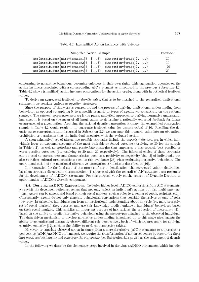
Modelling Dynamic Normative Understanding in Agent Societies 365
Table 4.2: Exemplified Action Instances with Valences
Simplified Action Example Feedback
act(attributes({name={trader1}}, {...}), aim(action={trade}), ...) 30act(attributes({name={trader2}}, {...}), aim(action={trade}), ...) 10act(attributes({name={trader3}}, {...}), aim(action={trade}), ...) -20act(attributes({name={trader4}}, {...}), aim(action={trade}), ...) 20
conforming to normative behaviour, becoming enforcers in their own right. This aggregation operates on theaction instances associated with a corresponding AIC statement as introduced in the previous Subsection 4.2.Table 4.2 shows (simplified) action instance observations for the action trade, along with hypothetical feedbackvalues.
To derive an aggregated feedback, or deontic value, that is to be attached to the generalised institutionalstatement, we consider various aggregation strategies.
Since the purpose of this work is centred around the process of deriving institutional understanding frombehaviour, as opposed to applying it to a specific scenario or types of agents, we concentrate on the rationalstrategy. The rational aggregation strategy is the purest analytical approach to deriving normative understand-ing, since it is based on the mean of all input values to determine a rationally expected feedback for futureoccurrences of a given action. Applying the rational deontic aggregation strategy, the exemplified observationsample in Table 4.2 would result in an aggregate feedback value (or deontic value) of 10. Recalling the de-ontic range conceptualisation discussed in Subsection 3.2, we can map this numeric value into an obligation,prohibition or permission that the individual associates with the evaluated action.
A (non-exhaustive) set of alternative possible strategies include the opportunistic strategy, in which indi-viduals focus on extremal accounts of the most desirable or feared outcome (resolving to 30 for the samplein Table 4.2), as well as optimistic and pessimistic strategies that emphasise a bias towards best possible orworst possible outcomes (i.e. resolving to 30 and -20 respectively). The informed choice of those strategiescan be used to express personal characteristics, such as a positivity or negativity bias [5] of individuals, butalso to reflect cultural predispositions such as risk avoidance [23] when evaluating normative behaviour. Theoperationalisation of the mentioned alternative aggregation strategies is described in [16].
In preparation for the final step of this process of norm identification, the aggregated value – determinedbased on strategies discussed in this subsection – is associated with the generalised AIC statement as a precursorfor the development of nADICO statements. For this purpose we rely on the concept of Dynamic Deontics tooperationalise nADICO’s Deontic component.
4.4. Deriving nADICO Expressions. To derive higher-level nADICO expressions from AIC statements,we revisit the developed action sequences that not only reflect an individual’s actions but also multi-party ac-tions. Actors can be generalised based on their social markers, such as roles (e.g. sender of goods, recipient, etc.).Consequently, agents do not only generate behavioural conventions that consider themselves or only of rolesthey play. In principle, individuals can form an institutional understanding about any role (or, more precisely,set of social markers) they observe, and use this knowledge predict unknown individuals’ behaviours basedon their social markers. This satisfies an important purpose of institutions, the reduction of uncertainty [31],based on the ability to predict normative behaviour using the stereotypes attached to the observed individual.The data-driven mechanism to develop normative understanding introduced up to this stage gives agents theability to generalise and abstractly observe different role perspectives, both of which are precursors for applyingcognitive empathy [12], such as the ability to perform perspective taking.
However, to translate observed action instances from a mere descriptive (AIC statements) to a prescriptiveperspective (ADIC/nADICO statements), we require the transformation of action sequences by separating thoseinto monitored statements and consequential statements (see Subsection 3.1) as well as the assignment of deonticvalues.
In the following we describe the elementary steps involved in deriving nADICO statements, which include:

366 C.K. Frantz, M.K. Purvis, B.T.R. Savarimuthu and M. Nowostawski
• Identification of monitored and consequential statements• Assigning the deontic value to the monitored statement• Inverting the deontic value and assigning it to the consequential statement
Identifying Monitored and Consequential Statements. In the course of their interaction, individuals collectaction sequences, i.e. actions along with preceding actions, expressed as act statements with a subsequent actstatement’s conditions component (see Subsection 4.1). These action sequences represent action/reaction pairsthat describe a ‘because of’, or ‘on the grounds of’ relationship, reflecting a direct causal dependency betweenboth actions. Using our running example we would then arrive at the interpretation: “The Maghribi operatortrades goods because he has been sent goods by the Maghribi sender.”, which represents the descriptive normperspective directly derived from observed behaviour. However, to represent an injunctive perspective thathighlights an individual’s perception of its duties [10], we require the transformation into ‘Or else’ relationshipsfor cases in which multiple actions occur in sequence. An example of such generalised action sequence is theinitial statement ‘Sender sending goods’, followed by ‘Operator trading goods.’. To reflect the injunctive natureof the ‘Or else’, we attach textual representations of perceived duty (deontics) to the individual statements andinvert the derived consequential statement’s deontic (‘Senders have to send goods, or else Operators will NOTtrade goods.’). As discussed in Subsection 3.2, note that the deontic terms associated with the deontic range(may, should, must) may not precisely reflect this understanding, but they capture the intuition of varyinglevels of duty.
To proceed along these lines, it is necessary to identify action sequences that involve one’s social environ-ment, i.e. multi-party interactions. Operationally, starting from the last element in the action sequence (i.e. themost recent action), the agent iterates backwards through the action sequence and identifies the first actionstatement whose attributes (i.e. generalised social markers) differ from the final action statement’s attributes.The subsequence of all remaining action statements is then treated as monitored statement (i.e. the statementwhose compliance is monitored), whereas the sequence of all parsed action statements is interpreted as conse-quential statement. Let us use the following example to explore these mechanics: ‘Senders send goods’, followedby ‘Operators cheating’, followed by ‘Senders firing them’. Working our way backwards from the last statement(‘Senders firing them’), we find that the second last statement has a differing generalised actor (Operators),leaving us with the monitored statement ‘Operators cheat after Senders sending goods’ and the consequentialstatement ‘Senders firing them’.
If an action sequence does not include multiple parties, i.e. all actions are performed by a single individual(or multiple individuals carrying identical social markers), the last elementary action is then interpreted asthe previous action’s consequence and treated as consequential statement, with the preceding action statementsbeing the corresponding monitored statement.
Assigning Deontic Value to Monitored Statement. To give the statements normative value, we utilise theaggregated deontic value for the entire action sequence derived as part of the previously described feedbackaggregation step (Subsection 4.3) and assign it to the identified monitored statement’s Deontic component.
Assigning the Inverted Deontic Value to the Consequential Statement. Finally, to establish a deontic term’scorresponding counterpart (e.g. should vs. should not), we rely on the individual’s existing deontic range to invertthe aggregated value. The inversion involves the proportional mapping of deontic values along the individual’sdeontic range to the inverted deontic compartment. The resulting deontic value is assigned to the consequentialstatement to express the presumed consequence for the violation of the inferred monitored statement. Forexample, assuming a deontic range with midpoint value of 0, a value of 5 – possibly mapping to should – isinverted to its opposite scale value and deontic term (should not) as schematically visualised in Figure 4.5. Notethat the assumption of a symmetric deontic range is an exemplary simplification.11
11Alternative configurations are discussed in [16].
Modelling Dynamic Normative Understanding in Agent Societies 367
Fig. 4.5: Exemplified Deontic Inversion Process
Applying the deontic inversion to our running example, the corresponding nADICO statement reads:
adico(attributes({role={sender}, occupation={trader}}),deontic(5),
aim(action={send}, {object={goods}, target={attributes({role={operator}, occupation={trader}})}}),
conditions(*),
orElse(adic(attributes({role={operator}, occupation={trader}}),deontic(-5),
aim(action={trade}, {object={goods}}),conditions(*))))
Let us summarise the individual steps in algorithmic form.Using adick to describe an individual action statement at the k-th position within a sequence of statements
(adick)max
k=1(with the first statement being the last performed action and max indicating the total number of
action statements in the sequence), we can derive the corresponding nADICO statement nadico and define theassociated monitored statement (Function nadic(nadico)) and consequential statement (Function o(nadico)) asdescribed in Algorithm 2.
In the context of the derivation of nADICO statements, it is important to highlight a special case. Thisderivation approach does not establish a consequential statement if no previous action has been observed, gener-ating an injunctive norm without specified consequences, e.g. an obligation or prohibition without consequence.This corresponds to an ADIC statement in the nADICO syntax.
At this stage, the derived nADICO statements provide the experimenter with a comprehensive insightinto individuals’ experience-based normative understanding. The derived statements can be further generalisedbased on individual grammar components, such as
• actions (AIms) – by inferring an overall normative understanding of actions from aggregated nADICOstatements – and
• social structures (Attributes) – by generalising normative behaviour for specific actor stereotypes (e.g.roles) on multiple generalisation levels (e.g. by occupation, by origin, etc.).
However, as in reality, this mechanism can only operate on action sequences known to an agent, i.e. actionsan agent actually perceived. To afford the representation of deceitful behaviour and the associated informationasymmetry, we assume that some actions are performed internally without being directly accessible to outsideobservers. Agent can thus perform more actions than can be perceived by observers. An example is the action ofcheating, which may well be internalised by the cheating party, but will not be visible to the subject of cheating.Operationally, agents achieve this by internally maintaining action sequences that include the private actionsthey performed in addition to the publicly visible ones. The generalisation process itself is indifferent about thepublic or private nature of action statements in action sequences and operates on whichever statements havebeen perceived by the individual agent, potentially leading to an information asymmetry between the cheater(who knows he cheated) and the unknowing observer.
At this stage we will explore the introduced mechanism using the simulation scenario described at the outsetof this article.

368 C.K. Frantz, M.K. Purvis, B.T.R. Savarimuthu and M. Nowostawski
Algorithm 2 nADICO Statement Derivation Algorithm1: // 1 is last (i.e. latest) statement in sequence, max is first (oldest)2: k = 1;3: if max == 1 then4: // Only one statement in sequence5: // Assign monitored statement6: nadic(nadico) = adic1;7: // Assign aggregated feedback value (see Subsection 4.3) as monitored statement’s deontic8: d(nadic(nadico)) = d((adick)
maxk=1 );
9: else10: // More than one statement in sequence11: // Iterate backwards until attributes in statements differ12: while a(adick) == a(adick+1) & k < max do13: k++;14: end while15: if k == max then16: // Make last statement consequential statement if no deviating attributes found17: k = 1;18: end if19: // Assign subsequence from last (i.e. most recent) action statement to action statement k as
consequential statement20: o(nadico) = (adicl)
kl=1;
21: // Assign all other action statements as monitored statement22: nadic(nadico) = (adicl)
maxl=k+1;
23: // Assign aggregated feedback value (see Subsection 4.3) as monitored statement’s deontic24: d(nadic(nadico)) = d((adick)
maxk=1 );
25: // Assign the inverted deontic to consequential statement26: d(o(nadico)) = inv(d(nadic(nadico)));27: end if
5. Simulating Normative Understanding amongst Maghribi Traders. The Maghribi trader societyhighlighted in the beginning of this article provides an example of a medieval society that flourished based oninformal cooperation – without the use of existing centrally enforceable institutional instruments (such ascontracts). The mechanism described in this work thus bears characteristics that are compatible with thisprototypical scenario, that is the decentralised nature, the informal normative perspective, and the puristapproach towards inference of norms from experience and observation. We use this scenario to highlight thefeatures of this approach, specifically the ability to inspect agents’ minds individually, but also to develop anunderstanding of the collective normative landscape. Instead of exploring the test scenario comprehensively, weexplore distributions of non-/cooperative behaviour under which general economic cooperation can be sustained,but more importantly, how it is reflected in the emerging normative understanding.
Traders, potentially acting as sender and operator establish a maximum number (maxRelationships) ofmutual trade relationships to other traders based on random requests, to which they then send goods. Thereceiver trades those goods at a profit that is determined by a fixed factor profitFactor.12 If initialised as cheater,the trader cheats by embezzling a fraction of the profit (as described below) and returns the remainder to theoriginal sender. Sending agents memorise a parameterised number of last returned profits (as action feedback),which they can query for specific individuals or across all their partners in order to decide on the correctness ofthe returned profit. In cases of presumed cheating, traders can fire the suspect and memorise it as a cheater, orreward it with wageFactor of the generated profit. The interactions represent actions of the structure introducedin Subsection 4.1, with preceding actions stored in the Conditions component, successively building up actionsequences that represent the comprehensive transactions between individual agents.
To reflect the ongoing trade relationship, rewards are represented as the accumulated profit from previousinteractions with the rewarding party (i.e. the profits a respective trader had generated for the service providerover time). If the operator’s cheating was not detected, the cheater adds the embezzled fraction as part of his
12We use a fixed factor since it simplifies the detection of cheating. The focus of this work does not lie in the evaluation of anagent’s ability to detect cheating, but to understand the impact of cheating on the emerging normative understanding producedby the generalisation process.

Modelling Dynamic Normative Understanding in Agent Societies 369
reward from a trade interaction. In the case of firing, the fired trader memorises the inverted trade value andassociates it with the action sequence.
For each transaction agents generate corresponding action sequences. To represent deceitful actions, agentsmaintain private actions which they include in their internalised action sequences in addition to the overtlyobservable actions, as alluded to in Subsection 4.4. If an operator cheats, he internalises the action ‘cheating’(in addition to ‘trading’) but merely indicate that he traded the goods. He can then monitor this actionsequence and internalise if his cheating (in combination with trading) was successful. Another case is thesuspected cheating (from the perspective of the original sender of the goods). If suspecting cheating by anobserved agent, the original sender can add the private action ‘cheating’ to his internalised action sequence ofthe observed individual without sharing this suspicion.
Based on their experience agents derive normative statements as outlined in the previous sections. Traderscan query the derived statements to guide their decisions whether to continue sending goods by aggregatingdeontic values for given actions (e.g. sending goods) across one’s overall experience. Given our characterisationof norms as continua, agents stop committing to actions such as ‘sending goods’ as soon at those actions appearundesirable from a normative perspective. Using the labels of the prototypical deontic range (see Subsection3.2), this would be the case if such actions are associated with the deontic compartments may not, should not,or must not. However, instead of having agents rigidly act according to those compartments, we introduce anelement of randomness. To achieve this all deontic values are normalised across the deontic range (i.e. lowestdeontic value to 0 (must not), deontic centre as 0.5 (neutral), and highest deontic value as 1 (must)). Thosenormalised values are then used as input probabilities for the random number generator to determine whetherthe behaviour is performed (and economic transactions sustained). Defecting from performing such actionsnaturally limits market interactions if they are deemed normatively undesirable. In consequence, this affectsthe overall economic performance, with the best possible case being complete market participation, and theworst case being the breakdown of any market activity. The notion of normalised deontic values is likewise usedto determine the fraction of embezzled profits – the embezzled fraction increases with the internalised normativedesirability of cheating.
Algorithm 3 outlines the agents’ execution cycles described in the previous paragraphs; Algorithm 4 specifiesagents’ reactions to possible types of incoming requests (which are marked as different ‘cases’).
Algorithm 3 Agent Execution Cycle1: if < maxRelationships relationships to other traders then2: Pick random another trader this agent does not have relationship with and send relationship
request;3: if request is accepted then4: Add accepting trader to set of relationships;5: end if6: end if7: if agent has relationships to other traders then8: Pick random fellow trader from set of relationships;9: Determine random Boolean to decide whether to send goods (using normalised deontic
value for action ‘send goods’ as probability);10: if sending goods then11: Send goods to selected trader and await return of profit;12: if profit < 0 and mean value of memorised past transactions from trader is < 0 then13: Extend received action statement with action cheat;14: Memorise trader as cheater;15: Fire trader;16: else17: Reward trader by paying a reward of wageFactor ∗ profit;18: end if19: Memorise action statement in association with profit;20: end if21: end if22: Derive nADICO statements from memory;

370 C.K. Frantz, M.K. Purvis, B.T.R. Savarimuthu and M. Nowostawski
Algorithm 4 Agent Reactions1: Initialisation: Initialise agent as cheater with probability pcheater;2: Case 1: Receipt of Relationship Request3: if requester is not memorised as cheater and < maxRelationships relationships then4: Accept request and add requester to relationships;5: else6: Reject request;7: end if8: Case 2: Receipt of Trade Request9: Perform market transaction (goods’ value ∗ profitFactor);10: if initialised as cheater then11: Determine fraction f of profit to embezzle as normalised deontic value for action ‘cheating’
(0 < f ≤ 1);12: Create private copy of action statement and add action cheat;13: Memorise extended action sequence;14: end if15: Return (remaining) profit to sender;16: Case 3: Receipt of Firing Notification17: Remove sender from own relationships;18: Mark sender as cheater;
6. Evaluation. Turning to the evaluation, we develop a baseline scenario (Subsection 6.1) in order tounderstand how the generalisation mechanism can be operationalised. Following this, we modify the parameterset of the base model by introducing cheating (Subsection 6.2) and analyse how this affects the overall simulationoutcome. As a third step, we change the composition of the artificial society to see the impact of changingsocial structures on the emerging normative understanding (Subsection 6.3), before exploring the generalisationof norms beyond the observed actor characteristics as a precursor for predictive capabilities (Subsection 6.4).
6.1. Establishing Normative Understanding in the Base Scenario. We initialise the simulationwith the base parameter set outlined in Table 6.1, one of which we vary in the course of the evaluation. Sinceour intent is to measure economic cooperation, we use the number of performed transactions per round as atarget variable to indicate overall economic performance. With the exception of the wageFactor that is derivedfrom documented profit distributions in commenda relationships [44], the chosen parameter set has not beenempirically explored. Instead it is initialised to produce return for both sender and operator in the case ofcooperative interaction to show how such outcomes are reflected in the generated normative understanding,without assuming an accurate representation of historical happenstance.
Table 6.1: Simulation Parameters
Parameter Default Value Variation in Section
Number of Agents 50maxRelationships 20profitFactor (Factor of Goods’ Value) 1.3wageFactor (Factor of Total Profit) 0.33pcheater (Fraction of Cheaters) 0 Subsection 6.2Deontic Aggregation Strategy RationalNumber of Profit Memory Entries 100Number of Cheater Memory Entries 10
Running a base scenario without any cheating we can establish the maximum level of cooperation, that is100 transactions per simulation round. In this scenario each agent is involved twice per round, once for sendinggoods to initiate trade by another agent, and once for returning goods to the original sender. For all simulationruns we evaluate the emerging normative understanding after 1000 rounds, a period after which behaviourstabilised in all simulation scenarios.

Modelling Dynamic Normative Understanding in Agent Societies 371
In the base scenario the absence of cheaters offers limited surprise. However, it is a good starting pointto identify how our generalisation mechanism translates individual agents’ observations into normative under-standing at large. Inspecting an individual’s traces in Figure 6.1, we can identify the situational deontic rangeboundaries as well as the generated nADICO statements.
Fig. 6.1: Situational nADICO Statements for Individual Agent in Baseline Scenario
For this particular agent, the deontic range spreads from around -13.73 to +28.11, with the deontic centrelying at 0. The subranges from centre to proscriptive end, and from centre to prescriptive end are divided intoequally-sized deontic compartments within the respective subranges.
Based on its experience this particular agent has inferred two nADICO statements, both of which areidentified by indices. The essential features, such as actor attributes, deontic, and actions (aim) are highlightedto ease the interpretation. The statements consist of monitored statements on nesting level 0 (L0) that includesall preceding actions, as well as consequential statements, nested on Level 1 (L1), that attach an experientiallyderived presumed sanction for non-compliance. Translating the first statement into natural language, we canread ‘Operators may want to return profit (Line 1 of Statement 1), after having been sent goods by senders(Line 3) and traded those (Line 2), or else senders must not reward operators (Line 4).’ As noted before,the preceding actions leading to the monitored action are stored in the Conditions component of a nADICOstatement on a given nesting level and may carry preceding actions on their own, as found in this example.
The second statement concerns the action ‘sending goods’ and reads: ‘Senders must send goods (Line 1 ofStatement 2), or else operators must not return profit (Line 2) after having traded those (Line 3).’
Both statements manage to capture the complexity of the interactions and role associations, while beingaccessible for human interpretation. However, even though both statements describe inferred obligations theirdeontic strength varies, with strong inclinations for sending goods (Statement 2) and initiating trade interactionsthemselves, while the return of profit (Statement 1) is of lesser priority. This is associated with the varyinglevels of reinforcement both actions experience based on the internalised feedback.
This aspect is better reflected when observing the normative understanding on the macro-level. For thispurpose we rely on a Kiviat-inspired chart that shows distributions across adjacent ordinally scaled values, suchas deontic terms associated with the individual deontic compartments. Figure 6.2 shows the distribution ofnormative understanding for identified nADICO statements, with focus on the monitored statements’ Attributescomponent (in our case ‘Operator’ or ‘Sender’ and further social markers), followed by the action sequence (tobe read in reverse order similar to the individual statements above, with the last action being the guardedaction in the monitored statement; the consequential statement’s action is omitted).
Observing the aggregated overview, we can see that the vast majority of agents (82%) feels obliged tosend goods, with a minor fraction of 18% perceiving it as omissible (generally obligatory, but exceptionallyforegone). Returning profit finds more moderate reinforcement, with 70% only feeling mildly inclined to do so,mostly because of the lesser feedback compared to the aggregated feedback from sending goods (which includesthe incurred profit). However, in all cases the normative understanding suggests economic cooperation. Thisexample highlights the relationship between reinforcement and the salience of a given norm for our generalisationmechanism, thus offering a possible approach to model the prioritisation of conflicting or alternative norms.

372 C.K. Frantz, M.K. Purvis, B.T.R. Savarimuthu and M. Nowostawski
Fig. 6.2: Distribution of Normative Understanding for Baseline Scenario
With this baseline in mind, we can introduce different levels of cheating into the social composition andobserve how this is reflected in the level of cooperation, as well as individuals’ normative understandings.
6.2. Modifying Behaviour: Introducing Cheating. To analyse the effect of cheating on the artificialsociety, we incrementally increase pcheater, i.e. the fraction of all agents that involve in cheating.
Introducing a fraction of 25% as cheaters, the society can still sustain nearly full cooperation (as shown inTable 6.2). This implies that the modelled society can sustain a moderate amount of cheating. However, togain insight into what exactly facilitates this, we can inspect the normative understanding shown in Figure 6.3,which, in addition to the previous figure, includes an additional third action sequence, reflecting experience ofcheating (to be read as ‘returning profit after having been sent goods, traded, as well as cheated’).
Observing the traces in the radar chart, we can see that the majority of agents has a stronger inclinationto trade fair (the blue trace) than to cheat. This dominant commitment to honour the operator’s obligation toreturn goods over cheating ensures the continued sending of goods (red trace), even though to a slightly lesserextent than in the baseline case (see Figure 6.2 in Subsection 6.1).
Only for higher levels of cheating we notice an incremental breakdown of market operations, with meantransactions counts for selected cheater fractions shown in Table 6.2. All statistical values are based on 30simulation runs per configuration.
Table 6.2: Transaction Counts for Different Cheater Fractions
Cheater Fraction Mean Std. dev.
0 98.873 5.1640.25 99.805 0.5650.5 84.378 5.3380.75 35.428 5.5441 11.442 4.485
More interesting than the breakdown of market cooperation are the means by which we can retrace this

Modelling Dynamic Normative Understanding in Agent Societies 373
Fig. 6.3: Distribution of Normative Understanding for a Cheater Fraction of 25%
shift in normative understanding. While cheating levels up to 0.5 only affect the priorisation of actions on theprescriptive part of the deontic range (see Figure 6.4(a)), higher levels afford a shift of the action ‘send goods’into the proscriptive range, thus promoting the undesirability of that action (red trace) as shown for a cheaterfraction of 75% in Figure 6.4(b). This shift is based on the declining revenue for initiating trades in the lightof increasing levels of cheating (note the desirability of cheating (green trace) over honest trading (blue trace))and thus the incremental breakdown of cooperation.
(a) Cheater Fraction of 50% (b) Cheater Fraction of 75%
Fig. 6.4: Distribution of Normative Understanding for Different Cheater Fractions
To get a better understanding of an individual agent’s motivation to adjust its behaviour, we can observethe generated statements for an individual trader in a scenario with a cheater fraction of 75% as shown in Figure6.5.
In this example, the agent has generated three nADICO statements, with the first one highlighting thedesirability of cheating, the second one indicating the undesirability of sending goods, and the third one indi-

374 C.K. Frantz, M.K. Purvis, B.T.R. Savarimuthu and M. Nowostawski
Fig. 6.5: Situational nADICO Statements for Individual Agent in Scenario with a Cheater Level of 75%
cating a moderate inclination to trade fair. We highlighted the essential Attributes components and actions formonitored and consequential statements. To emphasise the composite nature of the first statement (specificallyin contrast to the third one), we additionally emphasised the horizontal nesting of the composite action ‘tradeand cheat’ that precedes the returning of goods.
While the second and third statement bear limited novel insights, the first one clarifies the motivation as towhy cheating is desirable. Interpreted literally, the agent presumes that ‘operators must trade, cheat and returnthe profit, or otherwise they are not fired’. This essentially reflects the inferred expectation of being fired as aresult of cheating. However, even though the agent identifies this norm, it does not have any prior conceptionof what ‘cheating’ or ‘returning profits’ entails, but infers this based on long-term reinforcement. In this casethe accumulated net pay-off of cheating and potentially being fired afterwards exceeds the pay-off received fromtrading fair (third statement), which makes cheating a profitable option. This interpretation shows that agentsare able to identify the normative behaviour, while their actions choices remain utilitarian.
This collective shift in normative understanding with increasing penetration of cheating highlights the con-ditions under which cooperation can be sustained in this agent society, and beyond the quantitative evaluationof the dependent variable ‘transaction count’, gives us insight into the normative understanding on micro- andmacro-level.
6.3. Modifying Structure: Introducing Outsiders. To explore the impact of introducing a wider setof different social actors (as opposed to merely changing behavioural composition as done up to this stage),we introduce a secondary type of trader into the social pool. While the Maghribis’ economic success builton the successful use of informal institutional instruments, European societies predominantly relied on formalinstitutional instruments such as contracts [19]. They did so in the light of changing social composition of theirsocieties (especially in City States such as Genoa), lacking long-term commitment of individuals, and thus anincreased incentive to cheat – since only long-term employment would have provided the necessary incentive toact compliantly.13
We thus conceive a second prototypical group of traders that is more inclined to cheat14, which we will referto as ‘Genoese’. Note that this composition is synthetic. Historically, Maghribis and Genoese hardly engagedin trade interactions with each other [19].
With an initial fraction of 25% as Genoese (and otherwise non-cheating Maghribis), after 1000 roundswe arrive at a transaction level of around 49, i.e. effectively half of the possible transactions. The incrementalbreakdown for changing social compositions (in fraction levels from 0.0 to 1.0 in steps of 0.25 across 30 simulationruns each) is shown in Table 6.3.
To maintain an accessible representation of the normative understanding, we separate the aggregated state-ments for Maghribis and Genoese, with the Maghribi representation shown in Figure 6.6(a) and Genoese onein Figure 6.6(b).
13For an in-depth elaboration refer to [19] and [16].14For Genoese we induce higher cheating levels by increasing the fraction of embezzled profits by 20%.

Modelling Dynamic Normative Understanding in Agent Societies 375
Table 6.3: Transaction Counts for Different Fractions of Genoese
Genoese Fraction Mean Std. dev.
0 98.873 5.1640.25 48.997 9.480.5 35.52 6.9660.75 32.003 6.6341 8.11 3.501
(a) Maghribis (b) Genoese
Fig. 6.6: Distribution of Normative Understanding for Maghribis and Genoese
Observing the non-cheating Maghribis, we can see how committing to trade requests and returning thegenerated profits is considered an obligation, since it yields in promising returns. Due to the increasing cheatinglevels, sending of goods becomes increasingly undesirable as of the considerable risk of being cheated by theintroduced Genoese.
This complements with the impression of the Genoese traders. Genoese initiate the bulk of trade trans-actions, but have a clear preference for cheating, with 67% treating it as a should, with the same 67% ofinterpreting only mild inclinations for fair trading.
In essence, integrating two different trader society’s operating based on different institutional principlesshows interesting interaction patterns, which we can derive from the emerging normative understanding. TheMaghribis concentrate their honesty on a role as operators, i.e. pursuing Genoese’ trade dealings, while thishonest trading behaviour sustains the Genoese’ commitment to inject a moderate level of goods into the market,thus preventing the economic collapse. Maintaining this base level of fair trading by Genoese senders andMaghribi operators, Genoese operators can retain their preference for cheating.
These interdependencies become clearer when inspecting individuals’ normative understandings – this timefrom a Genoese perspective shown in Figure 6.7.
The produced set of statements is double in size than for the uni-cultural case. Recall that Level 0 generali-sation (as introduced in Subsection 4.2) operates on all social markers (nADICO’s Attributes), that now not onlydifferentiates senders and operators as roles, but further includes the marker ‘origin’ (Maghribi vs. Genoese),for which normative behaviour can be characterised.
Specifically statements 2 and 3 are of particular interest. Both describe the agent’s normative understandingof cheating in the context of trading goods and returning profits, but they do so for different attribute sets.Statement 2 highlights that a Genoese operator should return profit to a Genoese sender when embezzlingprofits, whereas when dealing with a Maghribi sender, cheating is strongly undesirable. For this case, the

376 C.K. Frantz, M.K. Purvis, B.T.R. Savarimuthu and M. Nowostawski
Fig. 6.7: Situational nADICO Statements for Individual Genoese Agent in Scenario with 25% Genoese
Genoese operator favours fair trading instead (Statement 5).To understand how this differentiation comes about, we recall the principles of evaluating cheating: agents
evaluate the situational profit for negative values, but also keep track of historical cheating both on individuallevel (i.e. past returned profits of individual agents) and global level (i.e. average across all past trade interac-tions), which makes the evaluation relative to the context agents interact in. For example, interacting within apool of cheaters the embezzling of profit is less likely to be identified, in contrast to a predominantly compliantenvironment. As mentioned above, Maghribis stop initiating trade interactions (by sending goods) over thecourse of the simulation as of declining pay-offs (since cheaters eventually learn that cheating is profitable). Inconsequence, since they only act as operators they are hardly subject to cheating. However, if cheating occursthey operate based on past observations (from their earlier experience of fair trading), which leads to improvedidentification of cheating, resulting in negative feedback for the cheater. The Genoese, in contrast, continue tooperate as senders in this mixed society and ‘got used’ to a moderate amount of cheating, which makes it lesslikely to identify and fire cheating individuals. Strategically, for Genoese it makes more sense to cheat their ownkind, than embezzling profits from non-cheating Maghribis.
6.4. Generalising Identified Behaviour. This introduced complexity provides grounds for more dif-ferentiated social behaviour, with agents learning about actions as well as their social environment. However,as seen in the previous example, this complexity reflects all known categories of social structures, but doesnot give agents the ability to predict or stereotype behaviour on a more general level. Currently, agents canpredict behaviour for ‘Genoese traders’ or ‘Maghribi traders’, but fail to characterise behaviour for traders moregenerally.
In Subsection 4.2 we proposed a conceptual solution by affording multi-level generalisation that system-atically aggregates normative understanding by subsets of social marker combinations. In Figure 6.8 we canobserve an extract (2 out of 6 statements) of the same individual’s understanding (as from Figure 6.7) on thehighest generalisation level, in our case Level 2 – the generalisation of two attributes (out of three ones in ourcase: role, origin, occupation).
The traces concentrate on generalisations from a Genoese perspective, and result in the aggregation of state-ments based on the marker ‘Trader’ or ‘Genoese’. Generalisation based on the category ‘Genoese’ produces the

Modelling Dynamic Normative Understanding in Agent Societies 377
Fig. 6.8: Extract of Situational nADICO Statements on Generalisation Level 2 for Individual Genoese Agentin Scenario with 25% Genoese
same results as for the Level 0 generalisation (see Figure 6.7), whereas an aggregation by ‘Trader’ integrates thepreviously separated statements for ‘Maghribi’ and ‘Genoese’. Focusing on the cheating behaviour (Statements1 and 2 in Figure 6.8), we find that Statement 2 corresponds to Statement 2 in Figure 6.7, while Statement 1 inFigure 6.8 is an aggregation of Statements 2 and 3 in Figure 6.7. For this example, we can now develop a moreabstract picture of normative behaviour: while cheating is a desirable strategy for dealings amongst Genoese,for traders in general (which includes trades with Genoese and Maghribis) the likeliness of being fired leads to amild disinclination (may not) from cheating. In principle, a Genoese trader could now ascribe this behaviouralstereotype to newly entering non-Maghribi and non-Genoese traders (e.g. Venetian traders), and avoid cheatingas of the anticipated negative consequence.
With this derived abstract understanding, we can reflect stereotyping capabilities that extend beyondthe ‘known’ of the individual. This approach thus facilitates the reduction of uncertainty when dealing withnewcomers, as well as providing a shortcut for decision-making, which offers the potential for an efficiencyincrease – both of which are functions characteristic for institutions [32, 50].
7. Summary, Discussion & Outlook. In this work we extend a comprehensive approach to modelnorm emergence and identification in artificial agent societies previously introduced in [15]. It builds on anexpressive institutional grammar that captures different types of institutions, including conventions, norms,and rules (Subsection 3.1). The essential benefits of this structure are a) its generic and unified nature (onerepresentation for different institution types), while b) providing what we believe is an acceptable compromiseof accessible interpretation by human observers, and c) capturing institutions with great detail, facilitated by

378 C.K. Frantz, M.K. Purvis, B.T.R. Savarimuthu and M. Nowostawski
notions of nested institutional statements.This structural representation is augmented with a continuous conception of normative duty, capturing
prohibitions, permissions, and obligations (Subsection 3.2). This not only facilitates a nuanced expression ofnorms and a better reflection of their evolution over time, but provides the foundation for prioritising conflictingnorms along a continuous and dynamically changing deontic range. This representation is individualised, thusreflecting individuality on the micro-level, while maintaining generalisability for macro-level inspection of thenormative landscape. This analysis of the normative landscape can be performed on arbitrary social aggregationlevels, i.e. for all agents (macro-level), specific sub-groups (meso-level), such as cheaters or non-cheaters, as wellas for an individual-centric micro-perspective.
Apart from a refinement of the aforementioned structures and their specification, the essential contributionof this work lies in the systematic formalisation of the norm identification process and its extension with amulti-level generalisation of behaviour that operates on an individual’s experience of its social environment.The mechanism attempts to reconstruct subconscious norm internalisation processes by relying on conceptssuch as (experiential or social) learning and multi-level generalisation (stereotyping).
The integrated use of both ‘structure’ (nADICO & Dynamic Deontics) and ‘process’ (Generalisation) hasbeen demonstrated in a multi-agent trader scenario in which agents generate experience-based normative un-derstanding that feeds back into their action decisions. As part of the evaluation we explored the impact ofcheating behaviour and structural diversity on the emerging normative understanding.
Our evaluation scenario is inspired by a realistic medieval scenario from the area of comparative economics,in which we explored the effect of cheating in societies that operate on different institutional principles, with onesociety being the Maghribi collective that relied on informal coordination mechanisms, and a second one, theGenoese, that inherently relied on formal coordination mechanisms to foster long-distance trade interactions.Even though the results themselves bear limited surprise with respect to the introduction of cheating – eventuallyeconomic cooperation collapses – the emerging normative understanding does. Using the proposed generalisationmechanisms we can shed light on the inner workings of individuals as well as the motivations that underlie theiraction selection, such as understanding why specific levels of cheating can be tolerated while sustaining economiccooperation. Another interesting finding relates to the hypothetical mixing of both societies, with Genoese goodssenders developing a normative preference to interact with compliant Maghribis, while preferring to cheat theirown kind when acting as operators. These conceptions cannot be validated, since no interaction between bothsocieties has been documented [19]. However, it sheds an interesting insight into what could have happened ifboth collectives had interacted, and perhaps even sketching a possible reason why they did not (or ceased to doso).15
Our approach aims to provide a pragmatic account of realistic norm identification processes as evident inhumans beings as well as non-human species. This is in contrast to human-inspired norm engineering approachesthat rely on additional assumptions, such as central coordinating entities to guarantee the identification ofefficient norms (as is the case with Morales et al. [28, 29, 30]), or explicit collective action processes to facilitateconsensus (as used by Riveret et al. [37]). In contrast to their work, our generalisation of social structures doesnot rely on prior knowledge, such as ontologies or the like, but is inferred as part of the norm identificationprocess – the individuals themselves derive structure from behaviour. As with human societies, our conceptionof social norms is inherently virtual. No central entity maintains or governs a social norm. Individuals sharenorms via continuous internalisation and socialisation processes, but the normative understanding only existson the micro-level. A system-wide identification of norms only occurs for evaluative purposes, a feature that isfacilitated by the expressive but uniform institution representations.
The proposed process bears strong generalisability characteristics, since it operates on the subconsciouslevel and makes minimal assumptions about agents’ cognitive capabilities; it merely requires a representation ofindividual and social markers, as well as actions and associated feedback specifications – equivalents of whichare found in most social simulation scenarios.
We further believe that this approach bears strong potential for customisation beyond scenario-specificmarker and action specifications, including different configurations of the deontic range (see Subsection 3.2), or
15Recall that the Maghribis stopped sending goods in the course of the simulation because of the Genoese cheating behaviour,but continued to facilitate trading for others.

Modelling Dynamic Normative Understanding in Agent Societies 379
the personality- and/or culture-dependent choice of feedback aggregation strategies (see Subsection 4.3).
Similarly, the means by which agents can attain normative understanding are not constrained to reinforce-ment learning, but could involve notions of imitation, social learning, or even explicit communication. The latterfurther opens the prospect of injecting institutional (i.e. normative and/or legal) prescriptions, thus comple-menting the bottom-up perspective as emphasised in this work with a top-down perspective. The generalisationmechanism itself can furthermore be combined with other components to form a more realistic cognitive agentarchitecture, or be ‘plugged into’ existing architectures and complement explicit reasoning capabilities (such asthe case with BDI-style architectures) with a subconscious norm generalisation process.
We believe that the proposed approach is an important contribution towards a more realistic representa-tion of institutions in general, and norms in particular, moving agents an incremental step closer towards acomprehensive representation of human behaviour in silico.
REFERENCES
[1] D. Acemoglu and J. Robinson. Why Nations Fail: The Origins of Power, Prosperity, and Poverty. Crown Business, NewYork (NY), 2012.
[2] G. Andrighetto, D. Villatoro, and R. Conte. Norm Internalization in Artificial Societies. AI Communications, 23(4):325–339,Dec. 2010.
[3] M. Aoki. Toward a Comparative Institutional Analysis. MIT Press, Cambridge (MA), 2001.[4] A. Bandura, D. Ross, and S. A. Ross. Transmission of Aggression through Imitation of Aggressive Models. Journal of
Abnormal and Social Psychology, 63(3):575–582, 1961.[5] R. F. Baumeister, E. Bratslavsky, and C. Finkenauer. Bad is Stronger than Good. Review of General Psychology, 5(4):323–370,
2001.[6] C. Bicchieri. The Grammar of Society: The Nature and Dynamics of Social Norms. Cambridge University Press, New York
(NY), 2006.[7] G. Bjornsson and R. Shanklin. Must, Ought and the Structure of Standards. In F. Cariani, D. Grossi, J. Meheus, and
X. Parent, editors, Deontic Logic and Normative Systems, volume 8554 of Lecture Notes in Computer Science, pages33–48. Springer International Publishing, 2014.
[8] S. Bradner. Key Words for Use in RFCs to Indicate Requirement Levels. https://www.ietf.org/rfc/rfc2119.txt, 1997. Accessedon: 1st December 2015.
[9] C. Castelfranchi. Minds as Social Institutions. Phenomenology and the Cognitive Sciences, 13(1):121–143, 2014.[10] R. B. Cialdini, R. R. Reno, and C. A. Kallgren. A Focus Theory of Normative Conduct: Recycling the Concept of Norms to
Reduce Littering in Public Places. Journal of Personality and Social Psychology, 58(6):1015–1026, 1990.[11] S. E. Crawford and E. Ostrom. A Grammar of Institutions. In Understanding Institutional Diversity, chapter 5, pages
137–174. Princeton University Press, Princeton (NJ), 2005.[12] J. Decety and J. Grezes. The Power of Simulation: Imagining One’s Own and Other’s Behavior. Brain Research, 1079(1):4–14,
2006.[13] C. Frantz, M. K. Purvis, M. Nowostawski, and B. T. R. Savarimuthu. nADICO: A Nested Grammar of Institutions. In
G. Boella, E. Elkind, B. T. R. Savarimuthu, F. Dignum, and M. K. Purvis, editors, PRIMA 2013: Principles andPractice of Multi-Agent Systems, volume 8291 of Lecture Notes in Artificial Intelligence, pages 429–436, Berlin, 2013.Springer.
[14] C. Frantz, M. K. Purvis, M. Nowostawski, and B. T. R. Savarimuthu. Modelling Institutions using Dynamic Deontics.In T. Balke, F. Dignum, M. B. van Riemsdijk, and A. K. Chopra, editors, Coordination, Organizations, Institutionsand Norms in Agent Systems IX, volume 8386 of Lecture Notes in Artificial Intelligence, pages 211–233, Berlin, 2014.Springer.
[15] C. Frantz, M. K. Purvis, B. T. R. Savarimuthu, and M. Nowostawski. Modelling Dynamic Normative Understanding in AgentSocieties. In H. K. Dam, J. Pitt, Y. Xu, G. Governatori, and T. Ito, editors, Principles and Practice of Multi-AgentSystems - 17th International Conference, PRIMA 2014, volume 8861 of Lecture Notes in Artificial Intelligence, pages294–310, Berlin, 2014. Springer.
[16] C. K. Frantz. Agent-Based Institutional Modelling: Novel Techniques for Deriving Structure from Behaviour. PhD Thesis,University of Otago, Dunedin, New Zealand, 2015. Available under: http://hdl.handle.net/10523/5906.
[17] A. Ghorbani, P. Bots, V. Dignum, and G. Dijkema. MAIA: a Framework for Developing Agent-Based Social Simulations.Journal of Artificial Societies and Social Simulation, 16(2):9, 2013.
[18] A. G. Greenwald and M. R. Banaji. Implicit Social Cognition: Attitudes, Self-esteem, and Stereotypes. Psychological Review,102:4–27, 1995.
[19] A. Greif. Institutions and the Path to the Modern Economy: Lessons from Medieval Trade. Cambridge University Press,New York (NY), 2006.
[20] D. Grossi, H. Aldewereld, and F. Dignum. Ubi Lex, Ibi Poena: Designing Norm Enforcement in E-Institutions. In P. Noriega,J. Vazquez-Salceda, G. Boella, O. Boissier, V. Dignum, N. Fornara, and E. Matson, editors, Coordination, Organizations,Institutions, and Norms in Multi-Agent Systems II, volume 4386 of Lecture Notes in Computer Science, pages 107–120,Berlin, 2006. Springer.

380 C.K. Frantz, M.K. Purvis, B.T.R. Savarimuthu and M. Nowostawski
[21] S. A. Haslam, N. Ellemers, S. D. Reicher, K. J. Reynolds, and M. T. Schmitt. The Social Identity Perspective Today:An Overview of its Defining Ideas. In T. Postmes and N. R. Branscombe, editors, Rediscovering social identity, pages341–356. Psychology Press, 2010.
[22] G. M. Hodgson. The Evolution of Institutions: An Agenda for Future Theoretical Research. Constitutional Political Economy,13(2):111–127, 2002.
[23] G. Hofstede, G. J. Hofstede, and M. Minkov. Cultures and Organizations: Software of the Mind. McGraw-Hill, New York(NY), 3rd edition, 2010.
[24] ISO. ISO/IEC 14977 – Information Technology - Syntactic Metalanguage - Extended BNF, December 1996. Accessed on: 1stDecember 2015.
[25] S. C. Johnson. Hierarchical Clustering Schemes. Psychometrika, 2:241–254, 1967.[26] F. Lopez y Lopez, M. Luck, and M. d’Inverno. Normative Agent Reasoning in Dynamic Societies. In N. R. Jennings, C. Sierra,
L. Sonenberg, and M. Tambe, editors, Proceedings of the 3rd International Joint Conference on Autonomous Agents andMulti-Agent Systems, AAMAS ’04, pages 535–542, New York (NY), 2004. ACM Press.
[27] J. Morales, M. Lopez-Sanchez, J. A. Rodriguez-Aguilar, W. Vasconcelos, and M. Wooldridge. Online Automated Synthesisof Compact Normative Systems. ACM Trans. Auton. Adapt. Syst., 10(1):2:1–2:33, Mar. 2015.
[28] J. Morales, M. Lopez-Sanchez, J. A. Rodrıguez-Aguilar, M. Wooldridge, and W. Vasconcelos. Automated Synthesis ofNormative Systems. In Proceedings of the 2013 International Conference on Autonomous Agents and Multi-AgentSystems, AAMAS ’13, pages 483–490, 2013.
[29] J. Morales, M. Lopez-Sanchez, J. A. Rodrıguez-Aguilar, M. Wooldridge, and W. Vasconcelos. Minimality and Simplicityin the On-line Automated Synthesis of Normative Systems. In Proceedings of the 2014 International Conference onAutonomous Agents and Multi-Agent Systems, AAMAS ’14, pages 109–116, 2014.
[30] J. Morales, I. Mendizabal, D. Sanchez-Pinsach, M. Lopez-Sanchez, and J. A. Rodrıguez-Aguilar. Using IRON to BuildFrictionless On-line Communities. AI Commun., 28(1):55–71, 2015.
[31] D. C. North. Institutions, Institutional Change, and Economic Performance. Cambridge University Press, New York (NY),1990.
[32] D. C. North. Institutions. Journal of Economic Perspectives, 5(1):97–112, 1991.[33] T. Parsons. The Social System. Routledge, New York (NY), 1951.[34] C. S. Peirce. How to Make Our Ideas Clear. Popular Science Monthly, 12:286–302, January 1878.[35] E. A. Posner. Law, Economics, and Inefficient Norms. University of Pennsylvania Law Review, 144:1697–1744, 1996.[36] R. A. Posner and E. B. Rasmusen. Creating and Enforcing Norms, with Special Reference to Sanctions. International Review
of Law and Economics, 19(3):369–382, 1999.[37] R. Riveret, A. Artikis, D. Busquets, and J. Pitt. Self-governance by Transfiguration: From Learning to Prescriptions. In
F. Cariani, D. Grossi, J. Meheus, and X. Parent, editors, Deontic Logic and Normative Systems, volume 8554 of LectureNotes in Computer Science, pages 177–191. Springer, Springer, 2014.
[38] Y. Shoham and M. Tennenholtz. On the Synthesis of Useful Social Laws for Artificial Agent Societies. In Proceedings of the10th National Conference on Artificial Intelligence (AAAI ’92), pages 276–281, San Jose (CA), July 1992.
[39] Y. Shoham and M. Tennenholtz. On Social Laws for Artificial Agent Societies: Off-line Design. Artificial Intelligence,73(12):231 – 252, 1995. Computational Research on Interaction and Agency, Part 2.
[40] Y. Shoham and M. Tennenholtz. On the Emergence of Social Conventions: Modeling, Analysis, and Simulations. ArtificialIntelligence, 94(1–2):139–166, July 1997.
[41] S. Siddiki, C. M. Weible, X. Basurto, and J. Calanni. Dissecting Policy Designs: An Application of the Institutional GrammarTool. The Policy Studies Journal, 39(1):79–103, 2011.
[42] A. Smajgl, L. R. Izquierdo, and M. Huigen. Modeling Endogenous Rule Changes in an Institutional Context: The ADICOSequence. Advances in Complex Systems, 2(11):199–215, 2008.
[43] H. Tajfel. Social Identity and Intergroup Behaviour. Social Science Information, 13(2):65–93, 1974.[44] Q. van Doosselaere. Commercial Agreements and Social Dynamics in Medieval Genoa. Cambridge University Press, Cam-
bridge (UK), 2009.[45] D. Villatoro, G. Andrighetto, J. Sabater-Mir, and R. Conte. Dynamic Sanctioning for Robust and Cost-efficient Norm
Compliance. In T. Walsh, editor, Proceedings of the 22nd International Joint Conference on Artificial Intelligence,volume 1 of IJCAI’11, pages 414–419. AAAI Press, 2011.
[46] G. H. von Wright. An Essay in Modal Logic. North Holland, Amsterdam, 1951.[47] C. Watkins. Learning from Delayed Rewards. PhD thesis, Cambridge University, Cambridge (UK), 1989.[48] O. E. Williamson. Markets and Hierarchies, Analysis and Antitrust Implications: A Study in the Economics of Internal
Organization. Free Press, New York (NY), 1975.[49] O. E. Williamson. The Economic Institutions of Capitalism. Free Press, New York (NY), 1975.[50] O. E. Williamson. Transaction Cost Economics: How it works; Where it is headed. De Economist, 146(1):23–58, 1998.
Edited by: Hoa DamReceived: April 16, 2015Accepted: January 13, 2016

Scalable Computing: Practice and Experience
Volume 16, Number 4, pp. 381–401. http://www.scpe.org
DOI 10.12694/scpe.v16i4.1129ISSN 1895-1767c⃝ 2015 SCPE
A MULTI-AGENT APPROACH FOR TRUST-BASED SERVICE DISCOVERY AND
SELECTION IN SOCIAL NETWORKS
AMINE LOUATI, JOYCE EL HADDAD, AND SUZANNE PINSON∗
Abstract. Service discovery and selection approaches are often done using a centralized registry-based technique, which onlycaptures common Quality of Service criteria. With more and more services offered via social networks, these approaches are notable to evaluate trust in service providers and often fail to comply with new requester’s expectations. This is because thesesapproaches are not able (i) to take into consideration the social dimension and (ii) to capitalize on information resulting fromprevious experiences. To address these challenges, we propose the use of multi-agent systems as they have demonstrated thecapability to use previous interactions, knowledge representation and distributed reasoning, as well as social metaphors like trust.More precisely, in this paper, we enhance service discovery and selection processes by integrating the societal view in trust modeling.Based on relationships between agents, their previous experiences and extracted information from social network, we define a trustmodel built upon social, expert and recommender -based components. The social-based component judges whether the provider isworthwhile pursuing before using his services (viz. trust in sociability). The expert-based component estimates whether the servicebehaves well and as expected (viz. trust in expertise). The recommender-based component assesses for an agent whether one’s canrely on its recommendations (viz. trust in recommendation). However, when searching for a service in a social network, agents(service requester and service providers) may have no direct interactions or previous experiences. This requires a method to infertrust between them. Based on a probabilistic model, we estimate trust between non adjacent agents while taking into account roles(recommender or provider) of intermediate agents. Moreover, we propose a distributed algorithm for trustworthy service discoveryand selection using referral systems in social networks. Experiments demonstrate that our approach is effective and outperformsexisting ones, and can deliver more trustworthy results.
Key words: Service Discovery and Selection, Multi Agent System, Trust Model, Referral Systems, Social Networks.
AMS subject classifications. 68T42, 91D30, 90B22, 62F07
1. Introduction. More and more services are proposed via social networks (SN). In such context, arequester needs trustful and efficient methods to discover requested services given by trustees and to chooseamong them. Existing service discovery and selection approaches are generally based on non-functional servicedescriptions usually done through quality-driven techniques using QoS attributes and centralized registires (e.g.ebXML). In most of these approaches, trust in not considered ( [3, 8, 11]). Recent research works ( [28, 32, 38, 50])have shown that trustworthiness is a key factor for good service selection in order to comply with requester’sexpectations.
This paper proposes a new approach to discover and select services based on trust. Liu and Wang in [32]defined trust as “the belief of one participant in another, based on their interactions, in the extent to which thefuture action to be performed by the latter will lead to an expected outcome”. Several authors have proposedto integrate the societal view into the classical service discovery process [4, 9, 28, 31]. The societal view takesinto account various sources of trust information located in the social network of the trustor and considers pastinteraction between agents. Sabater and Vercouter distinguished in [44] three principal sources of informationthat agents can use to build trust: (i) individual experience between the trustor and the trustee which comesfrom a direct interaction between them, (ii) communicated experience which represents knowledge coming fromother agents describing their interactions with the trustee and, (iii) social information which may encompassesa variety of semantic and structural knowledge useful to evaluate trust (see Sect. 4 for description).
In this work, we propose to use a multi-agent system (MAS) to model the service discovery and selectionprocess where artificial agents represent requesters, providers and intermediate agents in the social network of therequester and interactions between agents are done through message exchange. Castelfranchi and Falcone [14]claimed that trust is a basis of interactions among artificial agents in multi-agent systems: one agent musttrust a counter-party to be willing to carry out interactions and delegate a task. Consequently, we design atrust model for social networks that 1) assists agents in identifying trustworthy service providers and 2) givesagents the ability to reason about trust in their distributed decision-making process. Our trust model is basedon real world characteristics of trust between people that are depicted in social science studies. Other fields are
∗ PSL, Universite Paris-Dauphine, LAMSADE CNRS UMR 7243 Paris, France, {amine.louati,elhaddad,pinson}@lamsade.dauphine.fr
381

382 A. Louati, J. El Haddad and S. Pinson
concerned with trust such as philosophy, socio-psychology and economics [2, 7, 36, 41]. All these fields showthat trust could have multiple components [1, 27] and that each component can play a specific role in assessingthe service trustworthiness. Some research works [29, 47, 51] focus on evaluating trust from a practical pointof view by means of a reputation measure. However, this expertise-based component of trust presents severallimits. As pointed out in [22, 42], trust evaluation comes from additional information sources different fromthose used in reputation computation such as social relationships between agents and their roles in the society.For example, [6, 32, 38, 43, 45] incorporate social network analysis as a part of the calculation of trust. Followingprevious works, our trust model is built upon three components namely trust in sociability, trust in expertise andtrust in recommendation (see Sect. 2 for a review). First, a high sociability value indicates relevant providersand good recommenders. The interest of such a component lies in evaluating trust in a provider without relyingon observations of other agents avoiding underlying subjectivity. Second, a high expertise value reflects thecapability of a provider to offer good services that behaves as expected. Finally, a high recommendation valuegives rise to good recommenders that one’s can rely on their opinion.
During the service discovery and selection processes, agents use the aforementioned trust components todecide with whom to interact. However, in absence of direct interactions, a social and decentralized approachnamely referral systems allow agents to cooperate by giving, pursuing and evaluating referrals [53]. In theliterature, a number of techniques for trust inference in social networks can be found [19, 21, 33, 48, 49] butthey usually focus on an evaluation based on a single trust value between adjacent agents regardless of theirroles in the chain. In this paper, we propose a distributed algorithm for service discovery and selection insocial networks that propagates trust values among agents using referral systems. Based on [48], we infer trustbetween non adjacent agents using a probabilistic model. This model takes into account roles (recommender orprovider) of intermediate agents along the chain. Experiments demonstrate that our approach is better than twowell-known trust methods, namely Bansal et al. [6], and Maaradji et al. [38], and can deliver more trustworthyresults.
The paper is organized as follow. In the Sect. 2, we present a literature review of different trust-basedapproaches for service discovery and selection in social networks. Sect. 3 defines the main concepts used inthis paper. Sect. 4 describes our trust model and its three components. In Sect. 5, we provide a detaileddescription of our trust-based discovery and selection approach. Sect. 6 discusses the experimental setup andthe performance evaluation of our approach. Finally, Sect.7 concludes and presents perspectives for future work.
2. Related Work. In the literature, most of the existing Web service discovery and selection approachesuse QoS attributes (e.g., latency, throughput, response time) to distinguish between functionally equivalent ser-vices. However, without trust consideration, selected services often fail to comply with requester’s expectations.In the following, we briefly review the relevant trust-based service discovery and selection related work fromthree viewpoints.
2.1. Trust-based expertise. Many works have evaluated providers’ trustworthiness from an expertiseperspective [9, 25, 29, 47, 51] aiming to improve the quality of the underlying composition. Vu et al. [47]presented a QoS-enabled distributed service selection framework including trust and reputation management.They use some dedicated QoS registries to collect QoS feedbacks from consumers. In [51], Xu et al. proposeda reputation-enhanced QoS-based Web service discovery algorithm for service matching, ranking and selectionbased on existing Web services. Billhard et al. [9] examined the problem of service provider selection usingan experience-based approach in which clients use confidence and reputation mechanisms to infer expectationsof future providers’ behavior from past experiences in similar situations. More precisely, when no previousexperience is available for a particular provider/service pair, authors proposed a way to estimate confidencevalues based on past experiences with similar services. Lalanne et al. [25] proposed an approach for usingquality of past experiences as a factor for service selection, including an analysis of the different factors thatmay affect the quality perceived by the end-user. Likewise, Li et al. [29] used users’ feedbacks including ratings,opinions and relevant comments after use to estimate service reputation. All of the above approaches haveevaluated trust from a subjective point of view based on the advertised QoS values.
2.2. Trust-based sociability. The expertise-based component evaluating trust between agents and ser-vices lacks social features, as for example relationships between users to make a significant assessment. To

A Multi-Agent Approach for Trust-based Service Discovery and Selection in Social Networks 383
address that, Da Silva and Zisman [17] proposed a trust model that takes into account different levels of trustamong users, different relationships between users, and different degrees of importance that a user may have forcertain QoS attributes. Some other works [6, 32, 38, 45] have investigated social network analysis techniquesto evaluate the trust in sociability an agent may have in a provider. Bansal et al. [6] for example, evaluateproviders’ trustworthiness based on the degree centrality that gives an indication of their prestige in the network.However, this is a poor definition of trust, since it just uses a single measure, the degree centrality. Maraadjiet al. [38], consider social proximity as an indicator to measure trust in sociability. Sierra used in [45] prestigeand centrality measures to compute the strength of information flow when there is no complete independencein the opinions expressed by agents. Recently, Liu and Wang presented in [32] a service provider selectionmodel considering both adjacent and end-to-end constraints, based on the quality of trust and a complex socialnetwork structure. This complex social network takes into consideration three concepts which are trust, socialrelationships and recommendation role reflecting better the real-world situations.
These works present several limits, most of them do not take into account the semantic information anddeal with social networks with only one type of relationships. To cope with these limits, we integrate in thepresent work semantic information by including profiles and relationship types between agents in trust modelingto enhance its effectiveness and expressiveness.
2.3. Trust-based recommendation. The goal of a trust-based recommendation system is to generatepersonalized recommendations by aggregating the opinions of users in the trust network. According to Golbeck[19], recommendation techniques that analyze trust networks provide more accurate and highly personalizedresults than other classical collaborative filtering techniques. Golbeck proposed a FilmTrust site for generatingpredictive movie recommendations from trust in social network. This trust-based movie recommendation isgrounded on knowledge extracted from annotations and user ratings added in the system. Hang and Singh [20]use a graph-based approach to recommend a node in a social network using similarity in trust networks. Al-Sharawneh and Williams developed in [5] an approach to model systems with autonomous interacting agents.Through a set of simulations, they investigated the impact of Goldbaum’s innovative “Follow the Leader”strategy in social networks in the context of Web service selection. They use a recommender system that guidesa user to select the best service that matches his requirements and preferences. Massa and Aversani [39] proposeda trust-based recommendation system where it is possible to search for trustworthy users by exploiting trustpropagation over the trust network [40]. Trust-based recommendation techniques provide a way of disseminatingtrust information within a social network which is the basis for inferring trust between non adjacent users.However, similarly to trust-based expertise approaches, they only depend on subjective information providedby users.
3. Preliminaries. We describe in this section the overall concepts used in this work, i.e., social networks,services, user needs, and software agents.
Social Networks. We consider a Multi-Relation Social Network (MRSN) [46] which takes into accountdifferent types of relationships linking two nodes. For example, in Fig. 3.1 there are three different relationshipsbetween nodes: family, friend, and colleague relationships. Unlike multiplex networks [30] that deal with multi-layered graphs defined over the same set of nodes where each layer represents a different relationship, we assumethat there is one single layer which contains different types of relationships. A multi-relation social networkis modeled by a graph, where nodes represent agents and, an edge between two agents indicates a symmetricsocial relationship between them. More formally, a multi-relation social network and neighborhood are definedas follows:
Definition 1. Given a set V = {a1, a2, ..., an} of agents and a set R of types of symmetric rela-tionships with R = {R1, R2, ..., Rr}, a multi-relation social network (MRSN) is a connected graph G =<
V,E1, E2, ..., Er > where Ei ⊆ V × V ∀i ∈ {1, ..., r} is the set of edges w.r.t the i-th relationship and∀i = i′, Ei ∩ Ei′ = ∅. Let ρ : E 7→ R be a function that links edges to the relationship they represent, i.e.an edge (ak, aj) ∈ Ei represents a social relationship of type Ri between ak and aj.
Definition 2. Given a MRSN graph G = (V,E), the neighborhood of an agent ak ∈ V w.r.t. a type ofrelationship Ri ∈ {R1, R2, ..., Rr}, denoted NRi
(ak), is defined as NRi(ak) = {aj ∈ V | (ak, aj) ∈ Ei}.
In the MRSN, each agent ak interacts with a subset of agents, called the social acquaintances SAk. This

384 A. Louati, J. El Haddad and S. Pinson
R1 (family)
R2 (friend)
R3 (colleague)
a0
a11 a
4a7
a2
a6
a5
a9
a8a
1
a3
a10
a12
s61, s62s63
s81 s91, s92
s121s21, s22
s51
s31s12
s71 s101s41s111
Fig. 3.1: Example of a MRSN
ak
PITk
Sk Prk
F=<s1, s2,…sl>
Fig. 3.2: Trust-based Agent Architecture
set represents ak’s local view in the MRSN such as SAk = ∪Ri∈R
NRi(ak).
Services. A service is described in terms of functionality, inputs, outputs, and non-functional attributevalues. We define a service as follows:
Definition 3. A service s is a n-uplet (in, out, f , q1, . . . , qd) where in is a set of inputs required to usethe service, out is a set of outputs provided at the completion of the service, f is a functionality describing theprovided capacity, and q1, . . . , qd are the advertised values of the d non-functional criteria.
User needs. A user communicates his needs by expressing a set of required services and his preferencesover relationship types and trust threshold values.
Definition 4. A query Q is a 5-uplet (F,U, α, β, µ) where F = {s1, s2, ..., sl} is a set of the requiredservices, U : R 7→]0, 1] is an utility function expressing user’s preferences over relationship types in the socialnetwork, α ∈ [0, 1] is a trust in sociability threshold, β ∈ [0, 1] is a trust in recommendation threshold andµ ∈ [0, 1] is a trust in expertise threshold.
The utility of a relationship Ri, where i ∈ N∗ is the rank of Ri in the preference order, can be defined as
follows U(Ri) =1
2i−1 . For example, consider the MRSN in Fig. 3.1 with three relationship types R1 = family,R2 = friend and R3 = colleague, and a user’s preferences over them such us family ≻ friend ≻ colleague.Therefore, U(R1) = 1, U(R2) =
12 and U(R3) =
14 .
Software Agents. We have chosen a deliberative architecture as in [12, 18] in order to enable agents toevaluate their trust in other agents before interacting with them. It is composed of four modules and two datarepositories as shown in Fig. 3.2. The four modules are: the reasoning module RM, the trust module T M,the control module CM and the interaction module IM. The two data repositories are: the belief repositoryBR and the goal repository GR.
Definition 5. An agent ak is defined as a 6-components structure < BR, GR, RM, T M, CM, IM >
with:• BR = <Prk, Sk, P ITk>, the belief repository with Prk a profile1, Sk = {sk1, . . ., skmk
} a set of offeredservices and PITk a Personal Interaction Table. Each record in PITk (see Tab. 3.1) contains thefollowing elements: an acquaintance agent aj ∈ SAk, the profile Prj of aj, the social acquaintances setSAj of aj and the set of services Sj provided by aj. This information is acquired through interactionsamong agents.
• GR, the goal repository which encompasses the required services needed to solve user’s query.
1A profile consists of a set of items structured into a set of fields, each field containing one or several values (e.g., gender=[female],music-likes=[folk, jazz, pop]).

A Multi-Agent Approach for Trust-based Service Discovery and Selection in Social Networks 385
Table 3.1: Personal Interaction Table Example (PIT0 of agent a0 in Fig. 3.1)
Acquaintance Profile Social Acquaintances Offered servicesa2 Pr2 SA2 = {a0, a1, a3, a5, a8, a12} S2 = {s21, s22}a3 Pr3 SA3 = {a0, a1, a2, a4, a11, a12} S3 = {s31}a4 Pr4 SA4 = {a0, a1, a3, a7, a8, a11} S4 = {s41}a5 Pr5 SA5 = {a0, a2, a8, a9} S5 = {s51}a6 Pr6 SA6 = {a0, a8} S6 = {s61, s62, s63}a7 Pr7 SA7 = {a0, a4, a8, a10} S7 = {s71}
• RM, the reasoning module representing the matching function. A matching function between a serviceskl ∈ Sk and a service s ∈ F is defined as follows:matching(s, skl) = True ⇔ (skl.in ⊆ s.in) ∧ (s.out ⊆ skl.out) ∧ (skl.f ≡ s.f).
• T M, the trust module which computes all trust measures that an agent ak has with its social acquain-tances before interacting with them.
• CM, the control module which manages agent’s behavior and guides its decision-making in the discoveryand selection process.
• IM, the interaction module which structures the messages built by the agent ak and handles the receivedones.
We now make some assumptions about agents and their behavior:
- Assumption 1. Agents are cooperative and have the good will to share their experiences with others.- Assumption 2. Agents have limited view in the social network, they only know agents that belong totheir social acquaintance set.
- Assumption 3. Agents perform decentralized decision-making in contacting other agents.
Agents are endowed with a bounded set of services and act on behalf of their associated users to discover andselect trustworthy providers with good services. During the service discovery process, some agents may be goodproviders and some others may not be good providers but may be well connected and thus, may recommendgood providers. We consider four different roles that an agent may have during the discovery process:
• requester: a requester is the agent that receives the query from its associated user containing therequired services. It is the initiator of the discovery and selection processes. It determines from itsacquaintances set the most trustworthy acquaintances and sends them the query.
• provider: a provider is an agent which offers one or many requested services. When an agent receivesa query, it determines how to fulfill it with its offered services. If there is a matching between desiredservices and offered ones, it claims to be a provider and participates to the search of other potentialproviders by propagating the query to its trustworthy acquaintances.
• recommender: a recommender is an agent which has no required services but may participate to thequery solving by discovering good providers. Unlike provider agent, a recommender agent queries onlytrustworthy acquaintances providing required services.
• stopper: a stopper is an agent that cannot participate to the query solving as it can neither providea service nor recommend a provider. In the discovery process, this role is seen as a lock that blocksthe query propagation in the social network. This allows us to limit the search space and reduce thecomputational cost.
4. Trust Model. This section presents our trust model for service discovery and selection processes insocial networks. First, we present the different sources of information that we used for trust evaluation. Then,we describe subsequently the three trust components of our model.
4.1. Sources of trust information. Trust is a complex social phenomenon which is the basis of all socialinteractions [1]. Thus, any computational model of trust must be designed based on how trust works betweenpeople in society. As stated in [44], trust models that use only one source of information usually fail to providea significant trust value of the trustee agent. Moreover, in a MAS context, trust evaluation is considered as an

386 A. Louati, J. El Haddad and S. Pinson
internal reasoning from different sources of information that leads the agent to build a belief about the behaviorof another agent [22]. For these reasons, we consider four different sources of information to build our trustmodel:
• Individual experience: It models the direct interaction between the trustor (i.e. agent which evaluates)and the trustee (i.e. agent which is evaluated). Based on its personal previous experiences, the trustorestimates how the trustee would behave in the current interaction. This type of information is used tocompute trust in recommendation and is a part of the calculation of trust in expertise.
• Communicated experience: In the individual experience we considered only the direct interaction be-tween the trustor and trustee. In the absence of direct interactions, indirect interactions or opinionsof other agents can be consulted. This mechanism is called the referral system, often used for locatingservices through trusted referrals.
• Social information: In addition to agent interactional history (which are used in the two previous typesof information), knowledge extracted from social networks can be a rich source for gathering information.Such information can be classified into two categories; semantic and structural. Semantic informationincludes trustor and trustee profiles and the relationship types between them. Structural informationare derived using social network analysis techniques. It encompasses the position of the trustee in thesocial network graph, the proximity between the trustor and trustee and their neighborhood structure.This information is used to evaluate the trust in sociability between two agents.
• Certified information provided by the trustee: In the previous cases, the trustor needs to collect therequired information itself. However, the trustee can also seek the trust of the trustor by presentingarguments about its trustworthiness. In this paper, such arguments are non-functional attributes (e.g.,reliability, specialization, and experience rating) of the different services that it offers. In contrast tocommunicated experience which needs to be collected by the trustor, the trustee stores and providessuch certified information on request to gain the trust of the trustor. As we mentioned before, a partof the calculation of trust in expertise is based on individual experience. The other part is based onthis type of information.
Our trust model integrates these four sources of information and it is able to provide a trust evaluationthat helps agents in their decision-making process when they want to interact. The problem of various sortsof disinformation and inaccuracy will be considered in future work. Integrating these various sources will alsoenhance the precision and the expressiveness of the trust model. This will be verified subsequently in ourempirical evaluation (cf. Sect. 6).
4.2. Trust in Sociability (ST). Trust in sociability evaluates the level of social trust an agent ak mayhave in another agent aj . It is computed by extracting information from MRSN such as the structure of thegraph, agents’ profiles that contain personal data and information about their interests, and relationship typesbetween agents. Based on the analysis of the MRSN graph and the extracted information, three measures arecomputed which are: the social position (SPo), the social proximity (SPr) and the social similarity (SSi). Next,we describe these measures, then we give the way to compute trust in sociability.
4.2.1. Social Position Measure (SPo). The social position of an agent aj is computed based on itsdegree centrality which represents its social power. In a single-relation social network, it is computed as thedegree of an agent (see for example [6]). In our work, we do not simply compute SPo(aj) as the number ofrelationships of agent aj , but we also consider relationship types {Ri, 1 ≤ i ≤ n} connecting aj to the otheragents as follows:
SPo(aj) =
r∑
i=1
∑
al∈SAj
U(ρ((aj , al)))× bi(aj , al) (4.1)
where bi(aj , al) = 1 iff aj and al are directly connected with an edge of relationship Ri, 0 otherwise.An agent with a high degree centrality has an important structural position in the social network because
the more interactions it has, the more prestigious it is in the social network. Therefore, we believe that agentswith a high degree centrality have a leading position and are considered trustworthy by other agents in thenetwork.

A Multi-Agent Approach for Trust-based Service Discovery and Selection in Social Networks 387
4.2.2. Social Proximity Measure (SPr). It is defined as the average cost of a path between two agentsin the graph. Since there are different kind of relationships {Ri, 1 ≤ i ≤ n} in the MRSN with preferencesassociated with them, we define SPr as follows:Let path = (ak, . . . , aj) be a path of length d between an agent ak and an agent aj , and U(ρ((al−1, al))) be thecost of the edge (al−1, al) ∈ path (see Def. 4).
SPr(ak, aj) =
∑dl=1 U(ρ((al−1, al)))
d(4.2)
In a single-relation social network, the shortest path between a pair of agents is the best path for socialproximity [38]. In a multi-relation social network and according to Eq. 4.2, proximity between two agentsdepends not only on the length of the path but also on semantic aspects, that is the type of links that composeit. In some cases, a longer path may have a better cost if it is composed of relationships preferred by the user.
4.2.3. Social Similarity Measure (SSi). The social similarity between two agents is computed basedon the comparison of their profiles and their social acquaintance sets. As demonstrated in [55], we believethat similarity between two agents goes beyond the similarity of their profiles and includes similarity of theirneighborhoods. SSi(ak, aj) is an aggregation of two measures, namely, Neighborhood Similarity (NS) and ProfileSimilarity (PS). First, we present NS and PS then we show how to aggregate them to compute SSi.
Neighborhood Similarity Measure (NS). As proved by Hang and Singh in [20], the number of common neigh-bors influences the trustworthy recommendation process. Thus, the higher the number of common neighborsbetween two agents, the higher the social intimacy degree between them. This is the case of Facebook whichrecommends friends based on the number of mutual friends between them. One of the fundamental principlein social psychology [41] is that an agent can trust more agents with intimate social relationships than agentswith less intimacy. Following this principle, we define a measure called neighborhood similarity to find linksbetween agents based on their social acquaintances as follows:
NS(ak, aj) =
|R|∑
i=1
U(ρ((al−1, al)))× δi(ak, aj) (4.3)
with δi(ak, aj) = 11+jaci
where jaci = yi+zixi+yi+zi
is the Jaccard distance between ak and aj according to the
relationship Ri such as xi = |NRi(ak) ∩NRi
(aj)|, yi = |NRi(ak)| − xi, zi = |NRi
(aj)| − xi.Profile Similarity (PS). In social networks, an agent’s profile is not only characterized by its acquaintances,
but also by a set of personal information (e.g., gender, work) and interests (e.g., games, music, movies). Wedefine a profile as follow:
- < Profil >::=< item >+
- < item >::=< field >+
- < field >::=< value >∗
We use this information to compute trust between agents taking into account the similarity of their profiles.As shown in [55], in a real online community, a correlation exists between the degree of trust between agentsand their profile similarity. The more two users trust each other, the more similar their profiles are. Based onthese findings, we define a measure called profile similarity as follows:
PS(ak, aj) =1
|I|×
∑
i∈I
βi × Si(ak, aj) (4.4)
where Si(ak, aj) is the similarity between the ith items of ak and aj using Burnaby measure [13], I is the setof items in profiles and βi is the weight attributed to the item i with
∑
i∈I βi = 1. For more details concerningitem similarity computation, readers are referred to our previous work [34].
The overall measure of social similarity, SSi(ak, aj), between a requester agent ak and an agent aj iscomputed as the product of the two above measures:
SSi(ak, aj) = NS(ak, aj)× PS(ak, aj) (4.5)
388 A. Louati, J. El Haddad and S. Pinson
4.2.4. Trust in Sociability Computation. ST between a requester agent ak and an agent aj is computedfrom SPo (Eq. 4.1), SPr (Eq. 4.2), and SSi (Eq. 4.5). Let Mj be a vector associated with each agent aj suchas Mj = (SPo(aj), SPr(ak, aj), SSi(ak, aj)). Let M be a matrix obtained by merging the Mj vectors of allacquaintances aj such as M = (Mjt, aj ∈ SAk and 1 ≤ t ≤ 3) in which each row Mj corresponds to an agentaj , and each column corresponds to a social measure. To compute the value of the trust in sociability for eachagent aj , we use a Simple Additive Weighting technique that proceeds in two phases:
• Scaling phase: which aims to transform each measure value, of Mj vector, into a value between 0 and1 according to the following formula.
M ′jt =
{
Mjt−Mmint
Mmaxt −Mmin
t
if Mmaxt −Mmin
t = 0
1 if Mmaxt −Mmin
t = 0(4.6)
where Mmaxt = Max(Mjt), ∀aj and Mmin
t = Min(Mjt), ∀aj are the maximal value (respectively theminimal value) of a column in the matrix M . Applying the formula 4.6 to M , we obtain a matrixM ′ = (M ′jt, aj ∈ SAk and 1 ≤ t ≤ 3), in which each row M ′j corresponds to an acquaintance aj , andeach column corresponds to a social measure.
• Weighting phase: which aims to give a social trust value to each acquaintance aj ∈ SAk. The overallsocial trust value is computed as follow:
ST (ak, aj) =3
∑
t=1
λt ×M ′jt(ak, aj) (4.7)
where λt ∈ [0, 1] is the weight of the t-th social measure with∑3
t=1 λt = 1.
4.3. Trust in Expertise (ET). Trust in sociability checks whether an agent is socially trustworthy ornot. However, it does not evaluate the relevance of its offered services. We think that building trust solely onthe basis of a social-based component is insufficient to lead to a good service selection. According to [4], whenan agent relies on another socially trustworthy agent there is still an amount of risk regarding the quality ofits offered services. The quality of the selection process can be improved further by assessing providers qualityof service called expertise. Based on this statement, we introduce another component of trust called trust inexpertise ET that considers the non-functional properties of a service. Therefore, a good agent should be notonly socially trustworthy but also sufficiently expert. Based on [25], we define a trust in expertise ET (ak, aj , sjl)that an agent ak has in a service sjl offered by an agent aj as the aggregation of three following non-functionalattributes.
1. Specialization (Sp): is the percentage of successful use of an agent’s service sjl compared to the otherservices it offers. It is defined as the ratio between the number of times that a service sjl has beensuccessfully completed [38] and the total number of successful executions of the agent aj regardless ofthe used service.
Sp(sjl) =Nbsuccess(sjl)
∑mj
t=1 Nbsuccess(sjt)(4.8)
where Nbsuccess(sjl) is the number of successful executions of sjl and mj is the number of servicesoffered by agent aj . This means that the more the service sjl is sought for in the social network themore aj is recognized as an expert in this field.
2. Reliability (Re): is the probability that a service sjl is operational at the time of invocation. It iscomputed as the rate between the number of successful executions Nbsuccess(sjl) and the total numberof functionality invocations Nbinvoc(sjl).
Re(sjl) =Nbsuccess(sjl)
Nbinvoc(sjl)(4.9)

A Multi-Agent Approach for Trust-based Service Discovery and Selection in Social Networks 389
3. Experience rating (Eval): is the rating of the service realization quality. After the execution of a servicesjl, an agent ak gives an evaluation ν ∈ [0, 1] of this execution reflecting its experience feedback as acustomer of this service.Unlike the previous attributes, the evaluation of this attribute results from a subjective perception. LetEval(ak, sjl) be the average of the experience ratings of sjl for n uses by ak.
Eval(ak, sjl) =
∑nx=1 νx
n(4.10)
For the cold start, we introduce a trust bootstrapping phase. The goal for trust bootstrapping phaseis to assign an initial trust value Evalini to the new services (i.e., n = 0). We consider two strategies:negative and positive bootstrapping. In the first strategy, Evalini ∈ [0, 0.5[ whereas in the secondstrategy Evalini ∈ [0.5, 1].
The overall trust in expertise ET (ak, aj , sjl) that an agent ak have in a service sjl offered by an agent ajis computed as follows:
ET (ak, aj , sjl) = Sp(sjl)×Re(sjl)× Eval(ak, sjl) (4.11)
4.4. Trust in Recommendation (RT). According to [19], two types of trust are needed to evaluate thereliability of an agent: trust in this agent and trust in its recommendations for a specific service. When anagent ak receives a recommendation from an agent aj , apart from the fact that it ensures that aj is sociallytrustworthy, it prefers also that aj recommendations are trustworthy [7]. We associate a trust value calledtrust in recommendation (RT) with a service recommendation made by an aj to ak. The estimation of therecommendation trustworthiness is done using previous experiences with the potential recommender duringpast compositions. We decompose trust in recommendation RT (ak, aj , spl) that an agent ak gives to anotheragent aj regarding the quality of its recommendations for a service spl offered by the provider ap into two parts:the objective part, [rkj |spl] ∈ [0, 1], which indicates the performance of aj in terms of the number of goodrecommendations for the service spl, and the subjective part, [qkj |spl] ∈ [0, 1], which reflects the satisfaction ofthe agent ak for recommendations given by aj concerning the service spl. Based on a formula given in [16], wedefine RT as follows:
RT (ak, aj , spl) =
{
1 if [rkj |spl] = 0 or [qkj |spl] = 0([rkj |spl] + 1)[qkj |spl] − 1 otherwise
(4.12)
As mentioned above, [rkj |spl] represents the ratio of the effective selection made by ak among the totalnumber of recommendations of aj for the service spl offered by the provider ap. Based on [37], [rkj |spl] isdefined as follows:
[rkj |spl] =
{
1 if Nbrecjk|spl = 0Nbselkj|spl
Nbrecjk|spl
otherwise(4.13)
where Nbrecjk|spl and Nbselkj|spl correspond to the number of times that aj has recommended the service sploffered by ap to ak and the number of times that ak has selected spl in the underlying composition, respectively.
However, [qkj |spl] indicates how much an agent ak is satisfied with the recommendations of aj concerningthe service spl offered by the provider ap. Given Eval(ak, spl) (Eq. 4.10), the experience rating of spl given byak after its execution, [qkj |spl] is defined as the average of the different ratings made by ak to spl after successfulexecutions:
[qkj |spl] =
1 if Nbselkj|spl = 0∑Nbselkj|spl
1Eval(ak,spl)
Nbselkj |splotherwise
(4.14)

390 A. Louati, J. El Haddad and S. Pinson
5. Trust-based Service Discovery and Selection Approach Description. In this section, we de-scribe the three steps that encompass our Trust-based Service Discovery and Selection approach (TSDS): servicediscovery, trust inference, and service selection.The service discovery step (Step 1) is an algorithm composed ofthree phases: trust in sociability computation as defined in Sect. 4.2, matching functionalities, and computingtrust in recommendation as defined in Sect.4.4. The output of this step as shown in Fig. 5.1 is a tree graphcalled Trust-Relation Social Network (TRSN) in which providers as well as recommenders are identified. Rela-tionships between agents in TRSN are weighted by a pair of values representing trust in sociability and trustin recommendation between them. The second step, trust inference (Step 2), enables the service requester toevaluate trust it has in each of the discovered providers in the TRSN. It consists of propagating trust valuesfrom each discovered provider along the chain until the service requester. The latter retrieves the propagatedtrust values as an input and uses them to infer its trustworthiness to each discovered provider. The output ofthis step is a Requester-Centered Social Network (RCSN) in which a relationship between the requester anda provider is weighted by a trust value representing the inferred trust of the requester in the correspondingprovider. The third step is the service selection one (Step 3). In this last step, the service requester ranksservices of discovered providers depending on the value of their trust in expertise as defined in Sect. 4.3. Onlyservices with trust in expertise value greater than a certain threshold will be selected.
Note that in both the discovery and the selection steps of our TSDS approach, different trust componentsare computed. Each trust component has a specific role in the process. Trust in sociability and trust inrecommendation used in Step 1 act as a first filter leading to a set of trustworthy providers and recommenders.Trust in expertise used in Step 3 enables the selection of good services among those offered by the discoveredproviders. This separation allows us to avoid missed opportunities during the service discovery step. If weconsider trust in expertise in Step 1, only trustworthy providers will be discovered during this step and asocially trustworthy agent that does not have a required service (i.e. a recommender) will not be discovered.However, in some cases, such a trustworthy agent may be well connected and thus, may recommend a goodprovider.
5.1. Step 1: Service Discovery. The aim of this step is to discover trustworthy providers through adistributed trust-based breadth-first search algorithm, namely Algo. 1. The inputs of this algorithm are theMRSN graph and a query Q = (F,U, α, β, µ). To start the algorithm, the requester agent ar assigns itself therequester role (roler = Req), sets to 0 its distance distr
2 in the provider-recommender chain3, and initializesthe set PSetr
4 to ∅ (see Algo. 1 lines 2− 4).
To start the tree construction, ar needs to ensure that queried agents are socially trustworthy. To performtrust computation, ar updates its Personal Interaction Table PITr (see Tab. 3.1) regarding current informationof each of its social acquaintance aj ∈ SAr (i.e., offered services Sj , social acquaintance SAj and profile Prj).To do that, ar sends a Request message to each aj ∈ SAr, (see Algo. 1 lines 5− 7).
The behavior of an agent ak5 is event-driven: the reception of a message triggers the execution of a
particular procedure. Upon receipt of a Request message, an agent ak replies with an Inform messagecontaining information about its offered services Sk, its social acquaintance SAk and its profile Prk (see Algo. 1lines 29 − 31). As a result of receiving an Inform message by an agent in SAr, the requester increments itsmessage counter and updates its Personal Interaction Table PITr (see Algo. 1 lines 32− 35). Once all informmessages have been received, ar begins trust computation phase in which it evaluates trust in sociability ofeach acquaintance aj based on the social measure values described in Sect. 4.2. Agents with trust in sociability
2 distk represents the distance of an agent ak in the provider-recommender chain to the requester agent ar (initially equals+∞).
3 A provider-recommender chain corresponds to a sequence of agents starting from the requester agent and leading to a providerin which all intermediate agents are either providers or recommenders.
4 PSetr is a data structure that contains for each discovered provider its offered services as well as trust values of the intermediateagents with their respective roles in the provider-recommender chain. This information is useful to infer trust that ar has in eachdiscovered provider.
5 The index k identifies the agent executing the code.

A Multi-Agent Approach for Trust-based Service Discovery and Selection in Social Networks 391
Algorithm 1 Distributed Trust-based Discovery AlgorithmVariables: rolek ∈ {⊥, Req, Pro,Rec, Stop}, distk ∈ {0, . . . , n}, countk ∈ {0, . . . , |SAk|}, LTAk a set of trustworthy potential providers,LRAk a set of trustworthy potential recommenders, τk is an array of stacks where each stack represents a provider-recommender chainsof a discovered service, PSetk a set of stacks τk[ ] one per discovered service, fatherk the predecessor agent in the chain to the requester,childk a list of agents representing children of ak in the tree.
1: procedure Propagation(F , U , α, β, µ)2: if (rolek == Req) then
3: distk ← 0;4: PSetk ← ∅;5: for all aj ∈ SAk do
6: Request(ak, aj , ∅); ◃ go to line 297: end for
8: wait (countk == |SAk|);9: countk ← 0;10: LTAk ← {aj ∈ SAk |ST (ak, aj) ≥ α};11: end if
12: if (rolek ∈ {Req, Pro}) then
13: for all aj ∈ LTAk do
14: if (∃s ∈ F and sjl ∈ PITk.Sj |matching(s, sjl) == True) then
15: Propagate(ak, aj , (F , U , α, β, µ, distk)); ◃ go to line 3616: else
17: if (∃s ∈ F |RT (ak, aj , s) ≥ fβ(distk)) then
18: Propagate(ak, aj , (F , U , α, β, µ, distk)); ◃ go to line 3619: end if
20: end if
21: end for
22: end if
23: if (rolek == Rec) then
24: for all aj ∈ LRAk do
25: Propagate(ak, aj , (F , U , α, β, µ, distk)); ◃ go to line 3626: end for
27: end if
28: end procedure
29: procedure Receive Request(aj , ak, ∅)30: Inform(ak, aj , (Sk, SAk, Prk)); ◃ go to line 3231: end procedure
32: procedure Receive Inform(aj , ak, (S, SA, Pr))33: countk ← countk + 1;34: PITk.set(aj , S, SA, Pr);35: end procedure
36: procedure Receive Propagate(aj , ak, (F , U , α, β, µ, dist)37: if (distk > dist + 1) then
38: distk ← dist + 1;39: fatherk ← aj ;40: Inform(ak, fatherk, child); ◃ go to line 6241: for all aj ∈ SAk do
42: Request(ak, aj , ∅);43: end for
44: wait (countk == |SAk|);45: countk ← 0;46: if (∃s ∈ F and skl ∈ Sk |matching(s, skl) == True) then
47: rolek ← Pro;48: τk[k].add(ak, skl);49: LTAk ← {aj ∈ SAk |ST (ak, aj) ≥ fα(distk)};50: Propagation(F , U , α, β, µ); ◃ go to line 1251: else
52: LRAk ← {aj ∈ SAk |ST (ak, aj) ≥ fα(distk) and ∃s ∈ F and sjl ∈ PITk.Sj |matching(s, sjl) == True};53: if (LRAk = ∅) then
54: rolek ← Rec;55: Propagation(F , U , α, β, µ); ◃ go to line 2356: else
57: rolek ← Stop;58: end if
59: end if
60: end if
61: end procedure
62: procedure Receive Inform(aj , ak, child)63: childk.add(aj);64: end procedure

392 A. Louati, J. El Haddad and S. Pinson
value greater than α threshold 6 are kept in the LTAr set (see Algo. 1 lines 8− 10).
An agent ak has to check before propagating the query to a trustworthy agent aj ∈ LTAk whether it couldparticipate or not to the query resolution. Either by offering a required service or if not, by being a potentialtrustworthy recommender. In both cases, ak sends to aj a Propagate message containing the user’s queryand its current distance (see Algo. 1 lines 12− 22). We use trust in recommendation threshold fβ(distk) duringservice discovery step to reduce the search space (i.e. visited agents) while ensuring recommendations given bytrustworthy recommenders.
An agent ak that receives a Propagate message, compares the received distance value with its currentdistance value distk. If the received value is less than its current distance value then, ak sets distk to thenew value (see Algo. 1 lines 37 − 38). This test condition allows to give the shortest trustworthy path treethat prevents cycles. Then, it sets its father value fatherk to the sender and sends to it an inform messagecontaining a child string (see Algo. 1 lines 39 − 40). Upon receipt of an inform message containing a child
string, the father adds to its childk list the identifier of the sender (see Algo. 1 lines 62 − 64). Thanks tothis Inform, each agent knows its children in the tree. After that, ak updates its beliefs and matches requiredservices against its own offered services Sk using the matching function (see Algo. 1 lines 41−46). The matchingresult could lead to two cases:
• ak has a service that matches a required service. In this case, ak sets its role to provider (rolek = Pro)and initializes its stack τk[k]
7 as follows: τk[k] = {ak, skl} where ak is its identifier and skl is itsoffered service. Next, ak determines the LTAk set (see Algo. 1 lines 47 − 48). To be in this set, anacquaintance aj ∈ SAk must have a trust in sociability value ST (ak, aj) greater than fα(distk) (seeAlgo. 1 line 49).Thereafter, ak executes the Propagation procedure that sends a Propagate messageto all acquaintances in LTAk (see Algo. 1 lines 50 and 12− 22).
• ak does not provide any of the required services, it determines LRAk set containing its acquaintanceswhich are not only trustworthy but also that offer one of the required services (see Algo. 1 line 52). IfLRAk set of ak does not contain relevant acquaintances (i.e. either they are not enough trusty to berecommended or they do not offer a required service) then, it stops the query propagation and sets itsrole to stopper (rolek = Stop) (see Algo. 1 lines 56 − 58). Otherwise, ak sets its role to recommender(rolek = Rec) and executes the Propagation procedure by sending a Propagate message to allacquaintances in LRAk (see Algo. 1 lines 53 − 55 and 23 − 27). In this case, although ak does notprovide any required service, it participates in the discovery process while leading to relevant agents.
The output of the first step is a tree called Trust-Relation Social Network (TRSN) as shown in Fig. 5.1 inwhich the requester is the root and the providers (black nodes) and recommenders (white nodes) are identified.The different provider-recommender chains allows to build a directed and acyclic graph where the requester isthe root and the distance of each discovered provider to the requester is the length of its chain. At this stage,providers are discovered on the basis of the functional aspect as well as of the degree of their sociability. So far, the non functional aspect expressed by the trust in expertise is not yet considered.
5.2. Step 2: Trust Inference. In social networks, an agent evaluates the trustworthiness of anotherbased on direct interactions with it. With the absence of direct interactions, a trust inference mechanism isapplied. This mechanism uses trust values along paths that connect two agents to come up with a singleevaluation. In this step, we first show how trust values are propagated via intermediate agents to infer trustbetween non adjacent agents then, we describe how to build a new tree graph called a Requester-Centered SocialNetwork (RCSN).
6fx(distk) = (1−x)×(1−e−distk
D )+k where D is the network diameter and x ∈ {α, β} is the function that updates trust thresholdvalue depending on the chain length d (for more details see [35]). The initial values fα(0) and fβ(0) correspond respectively to α
and β the preference of the requester’s query. These values are incremented locally by ak according to its distk. We believe that thelonger the chain is, the higher the requester’s sociability and recommendation value expectations are. Therefore, it is reasonableto adjust α and β values to the current search depth. This ensures high sociability and recommendation values for providers thatare discovered far away from the requester.
7 τk is an array of stacks. Each stack represents a provider-recommender chain of a discovered provider containing its offeredservice and trust values of the intermediate agents leading to it with their respective roles.

A Multi-Agent Approach for Trust-based Service Discovery and Selection in Social Networks 393
Fig. 5.1: Trust-Based Service Discovery and Selection Approach (TSDS)
Algorithm 2 Trust Values Propagation Algorithm
1: procedure TrustInference( )2: for all aj ∈ childr do
3: Inform(ar, aj , infer);4: end for
5: end procedure
6: procedure Receive Inform(aj , ak, infer)7: for all al ∈ childk do
8: Inform(ak, al, infer);9: end for
10: if (rolek == Pro) then11: Inform(ak, fatherk, τk[k]);12: end if
13: end procedure
14: procedure Receive Inform(aj , ak, τ)15: id← last(τ).getId()16: τk[id]← τ ;17: Upgrade(τk[id]);18: if (rolek == Req) then19: PSetk ← PSetk ∪ {τk[id]};20: else
21: Inform(ak, fatherk, τk[id]);22: end if
23: end procedure

394 A. Louati, J. El Haddad and S. Pinson
Function 1 Upgrade(τ)
1: if (τ.length() == 1) then2: role← Pro;3: else
4: role← top(τ).getrole();5: end if
6: if (role == Rec) then7: τ.push({rolek, ST (ak, aj), RT (ak, aj)});8: else
9: τ.push({rolek, ST (ak, aj), 1});10: end if
Trust Values Propagation. Recall that the output of the previous step is a tree where agents are eitherproviders or recommenders and relationships between them are weighted by a pair of values representing theircorresponding trust in sociability and trust in recommendation. In this second step, the requester ar startsa trust inference algorithm, called Algo. 2, by sending to each of its children in TRSN an inform messagecontaining an infer string (see Algo. 2 lines 1 − 5). An agent ak that receives such a message, sends in turneach of its children an inform message (see Algo. 2 lines 6 − 9). Additionally, if ak is a provider, then itsends its father in the tree an inform message with a copy of its τk[k] containing its identifier and one ofits offered services that matches one of the required services (see Algo. 2 lines 10 − 12). Upon receipt of aninform message containing a stack τ from its child aj (see Algo. 2 line 14), an agent ak determines the id of theprovider and applies an upgrade function (see Algo. 2 lines 15− 17 and Func. 1) as follows. Depending on therole of aj , ak inserts a new element in τk[id]. If aj is a recommender (see Func. 1 lines 6− 7), then ak upgradesτk[id] with {rolek, ST (ak, aj), RT (ak, aj)} where rolek is its role, ST (ak, aj) and RT (ak, aj) are respectivelyits trust in sociability and trust in recommendation to its child aj . If aj is a provider, then ak upgradesτk[id] with {rolek, ST (ak, aj), 1}. In this case, aj being a provider, it does not generate recommendations andtherefore RT (ak, aj) = 1 (see Func. 1 lines 8 − 10). Once the upgrading is done, if ak is the requester agent(rolek==Req), then it adds this stack to its PSetr = PSetr ∪{τk[id]} (see Algo. 2 lines 18−19). Otherwise, akis an intermediate agent in the chain, then it applies the same mechanism by transmitting its upgraded τk[id]to its father and so forth until the stack reaches the requester agent (see Algo. 2 lines 20− 23). An example oftrust values propagation in the TRSN of Fig. 5.1 from the provider a9 to the requester a0 is given in Fig. 5.2.
a9 a8 a6 a0
τ9[9] = (a9, s9l) τ8[9] = (τ9[9] + (Rec, ST (a8, a9), 1)) τ6[9] = (τ8[9] + (Pro, ST (a6, a8), RT (a6, a8, s9l)))
τ0[9] = (τ6[9] + (Req, ST (a0, a6), 1))
Fig. 5.2: A provider-recommender chain
At the end of Algo. 2, the requester set PSetr contains one stack for each discovered provider ap. Eachstack includes trust values (i.e. trust in sociability and trust in recommendation) of intermediate agents in thechain = (ar, ak, ak+1, . . . , ap).
Trust values propagation is essential to infer trust that the requester has in a provider although it has nodirect interaction with it. In the literature, several methods have been proposed for trust inference in socialnetworks [19, 21, 33, 49, 48]. Most of these works [21, 33, 49] propose well defined operators of aggregation toinfer trust between non adjacent agents stemming from different paths. In this work, we infer trust betweennon adjacent agents from the provider-recommender chain based on the probabilistic approach proposed in [48].Compared to [48], our contribution consists of integrating trust in recommendation in the calculations dependingon the role of intermediate agents in the chain. Using information stored in PSetr and the total probabilitylaw, trust of the requester ar in a provider ap along the chain (ar, ak, ak+1, . . . , ap−1, ap) is inferred as follows:

A Multi-Agent Approach for Trust-based Service Discovery and Selection in Social Networks 395
Trust(ar, ap) = P (ar)× P (ak|ar)× P (ak+1|ak)× . . .× P (ap|ap−1) (5.1)
where P (ar) = 1 denotes the trustworthiness of ar to itself. P (ak|ar) denotes the trustworthiness of ak fromar’s point of view. This is an aggregation of trust in sociability and trust in recommendation such as P (ak|ar) =ST (ar, ak) × RT (ar, ak) where, RT (ar, ak) = 1 if rolek = Pro. At the end of this phase, from PSetr set andEq. 5.1, ar infers its trustworthiness in each discovered provider in the TRSN network.
RCSN Construction. The aim of this phase is to build a new network from the requester ar point ofview. Based on the trust value Trust(ar, ap) for each discovered provider ap, we build the Requester-CenteredSocial Network (RCSN) modeled by a directed and weighted tree graph G′ = (V ′, E′), where V ′ is the set ofproviders and the requester, and E′ is the set of edges. An edge (ar, ap) ∈ E′ is a social trust relationshipbetween ar and ap and the weight of an edge (ar, ap) is the inferred trust value between them. Detailed resultsare stored in a data structure PSet∗r computed as follows:
F1 : PSetr → PSet∗r
τr[p] 7→ (τr[p], T rust(ar, ap))
where F1 is a function that takes as input each stack τr[p] of a discovered provider ap and adds it to Trust(ar, ap),its inferred trust.
5.3. Step 3: Service Selection. In the previous steps, the service requester ar has discovered a set oftrustworthy providers in the social network. This present step consists of sorting these discovered providers andselect the best to perform the service selection. After computing the trust in expertise ET, ar constructs anordered set PSelr using the following function:
F2 : PSet∗r → PSelr
(τr[p], T rust(ar, ap)) 7→ (τr[p], T rust(ar, ap), ET (ar, ap, spl))
where F2 is a function that takes as input each record of PSet∗r and adds it to the trust in expertise that arhas in ap. Then for each required service, ar selects providers that have a trust in expertise value greater thanµ as shown in Fig. 5.1.
6. Experimental setup and performance evaluation. In order to empirically evaluate TSDS, ourmulti-agent approach for trust-based service discovery and selection, we have developed a prototype usingJava 1.7 and the Jade8 multi-agent platform. The MRSN graph data was stored in a GML format9. Severalexperiments have been performed, and all of them were run on a 3.1GHz Core(TM) i5-2400 running windows7, with a 8Go of RAM. In the first series of experiments, we examine the performance of our service discoverystep by assessing its effectiveness and efficiency. In the second series of experiments, we focus on the evaluationof the performance of our service selection step. The performance review is carried out through a comparativestudy versus two trust-based approaches, Bansal et al. [6] and Maaradji et al. [38], on two criteria, utilityand requesters’ satisfaction. The aim of this evaluation is to check whether or not our TSDS approach helpsusers to acquire good providers an so, allows them to gain better utility and satisfaction comparing to otherapproaches. Note that none of the aforementioned approaches have presented experimental results that evaluatetheir performance.
6.1. Experimental setup. The testbed environment for evaluating our approach is a social network ofagents providing services (called providers) and agents using those services (called requesters). We focus on twonetwork families: small-world and scale-free networks. Small-world networks are defined as a family of graphs
8 Telecom Italia Lab. JADE 4.3 http://jade.tilab.com/.9 Graph Modeling Language, 1997, http://www.fim.uni-passau.de/en/fim/faculty/chairs/theoretische-informatik/projects.html10 http://snap.stanford.edu/data/egonets-Facebook.html

396 A. Louati, J. El Haddad and S. Pinson
exhibiting three properties: weak connectivity, strong clustering, and small diameter. Scale-free networks arenetworks following a power-law degree distribution, a model for describing the behavior of node degrees. Mostnodes in such networks have few edges, but a few nodes have much higher degree.
In the first part (Sect. 6.2), we run simulations on synthetic graphs fitting the small-world properties (themaximal path length in each of these graphs is seven hops). To do that, we generate 5 graph instances wherethe number of agents is equal to 1000 and the number of edges is equal to 6000. We consider 3 categories offunctionalities: transportation, accommodation and entertainment. In each of them we generates 5 differentservices. We equip randomly each agent with three different services, one from each category. Recall that arequester’s query is defined as (F,U, α, β, µ). For sake of simplicity, we suppose that requesters need only oneservice F = {s}. We vary the initial α’s value in [0, 1], while β and µ are both set to 0.4.
In the second part (Sect. 6.3), we conduct experiments on a real dataset which is Facebook dataset10
containing 4039 agents and 88234 edges. This dataset has been proved to possess the small-world [52] andscale-free [24] characteristics of social networks. We use the dataset WSDream 11 of [54] which contains 5825Web services distributed among all agents. Each agent is equipped with three different services. Similarly, forrequester’s query we suppose that requesters need only one service F = {s}. We set trust thresholds as follows:α = 0.6, β = 0.4 and µ = 0.4. In both datasets (real and synthetic), we consider three type of relationships{R1, R2, R3}. The requester’s preferences over relationship types are equal to U(Ri) =
12i−1 with i ∈ J1, 3K. For
non-functional values, we consider also the dataset WSDream of [54].
6.2. Performance evaluation of our service discovery step. Effectiveness consists of monitoring theaverage quality of providers’ expertise in terms of trust in expertise for different trust in sociability thresholdvalues. Efficiency consists of examining the distribution of the trustworthy discovered providers along theprovider-recommender chain. The goal of these two experiments is to determine the best trust in sociabilitythreshold as well as the provider-recommender chain length to enhance the service discovery results.
Effectiveness. This experiment evaluates the effectiveness of our service discovery step based on referralsystems. It allows us to estimate in advance the quality of discovered services for different ranges of trust insociability values. As experimental methodology, we consider the three following referral policies:
• referAll: an agent sends the query to all agents in its social acquaintances set. This is a special caseof referencing in which trust is not considered. This is similar to GNUtella’s search process [23] wherequeries are spread by flooding i.e. each agent forwards an incoming query to all of its neighbors if itdoesn’t have the required file.
• referTrust: only agents with sociability value above a predefined trust in sociability threshold arereferred. This means, the higher the trust threshold is, the smaller the number of discovered providersis. This policy corresponds to our approach.
• referBest: an agent refers a single agent with the best sociability value among its acquaintances. Thisis similar to Freenet’s routing for request messages [26], where each Freenet client forwards the requestto another that is the likeliest to have the required information.
Figure 6.1 illustrates the evolution of the average quality of the expertise (averaged over all graph instances)versus the variation of the α’s value of different policies. We limit the length of chains to five similar toGNUtella’s time-to-live value. During the simulation, each agent generates 5 queries resulting in 5000 queriesall together over which we compute the average value of the trust in expertise of discovered providers. ReferAllpolicy corresponds to the case where α’s value is set to zero. ReferBest policy is independent of α and remainsconstant for all values. It is interesting to note that, among the three policies, the referAll policy performs theworst and its average quality is equal to 0.27. This result can be justified given that trust is not considered.Trustworthy as well as not trustworthy providers are discovered which would substantially decrease the averagequality of the expertise. Furthermore, it is also interesting to note three important points about the evolutionof the average quality of the expertise of referTrust policy versus the variation of α’s value. First, as shownin Fig. 6.1, the best average quality of the expertise corresponds to a α’s value equals to 0.6. Thanks to thisfinding, we can consider this value as a reference which could be recommended to the requester before launchingthe service discovery process. Second, when α = 1, referBest and referTrust curves intersect. This is equivalent
11http://www.wsdream.net/dataset.html

A Multi-Agent Approach for Trust-based Service Discovery and Selection in Social Networks 397
0 0.2 0.4 0.6 0.8 10
0.2
0.4
0.6
referAll
Trust in sociability threshold α
Average
qualityof
expertise
referTrustreferBestreferAll
Fig. 6.1: Effectiveness of our service discovery step
1 2 3 4 5 6 7 8 9 10 11 120%
20%
40%
60%
80%
100%
Provider-recommender chain length
Percentage
ofdiscoveredproviders
α = 0α = 0.2α = 0.4α = 0.6
Fig. 6.2: Efficiency of our service discovery step
to keep in both policies a single agent, which is the most trustworthy one. Third, within the range of values[0, 0.6], the referTrust policy curve has an increasing slope (i.e. providers with a low sociability also have lowexpertise). This indicates the existence of a correlation between the sociability and the expertise of an agent.With the increase of α’s value, less trustworthy providers are found as the average value of the expertise qualityincreases. However, when the α’s value is high, this correlation is no longer relevant. In this case, agents aretoo selective and few trustworthy agents are queried. This means that for high α’s values, some providers withgood expertise are no longer discovered because there are no chain of trustworthy agents leading to them. Thisindicates that these providers are socially disconnected from the requester agent.
Efficiency. We study in this experiment the efficiency of the discovery step according to another experi-mental parameter which is the length of the provider-recommender chain. During the simulation, each agentgenerates 5 queries resulting in 5000 queries all together over which we compute the average number of thediscovered providers for different chain length.
Approaches which evaluate trust in social networks offer computational models based on social relationshipswhich are often inferred from long paths. To illustrate this point, we represent in Fig. 6.2 the distribution incumulative percentage of the discovered providers (averaged over all graph instances) depending on the length ofthe provider-recommender chain. For different α’s values, we note that the number of the discovered providersin requesters’ social acquaintances represents a small fraction (about 1%) of the total number of discoveredproviders. Some agents may not be good experts, but may be well connected and may recommend goodproviders hence the interest of referral systems in searching for providers. In our approach, sociability creditsthe ability to give good referrals. The propagation of the search is performed via navigation in the socialnetwork, which explains the increase of the number of discovered providers depending on chain length. It isalso interesting to note that there is a trade-off between the length of the provider-recommender chain and thenumber of discovered providers. As a matter of fact, there is six times more chances (from 14% to 80%) tofind a trustworthy provider in a chain length equal to 7 than in chain length equal to 3. However, the averagenumber of discovered providers tends to level off once the chain length reaches a certain point (here equal to 8)regardless of trust threshold value. Concretely, when the chain length goes beyond a certain limit, the remainingproviders are socially disconnected from the requester. Following these results, we can consider the length ofthe provider-recommender chain as a parameter that could be adjusted before launching the discovery process.Setting a maximum length of 7 for example gives us the possibility to control the scope of search which wouldsubstantially limit the computation cost.
6.3. Performance evaluation of our service selection step. In this section, we evaluate the perfor-mance and the benefit of our service selection step in terms of utility and requesters’ satisfaction through acomparative study including three different approaches. The idea is to note the values of the different non-functional attributes of the selected services for each approach. Then, we compare the performance of our

398 A. Louati, J. El Haddad and S. Pinson
three-step approach with (i) a one-step approach (i.e. Maaradji et al.) that aggregates trust in sociability andtrust in expertise as a single value in service selection, (ii) another one-step approach (i.e. Bansal et al.) thatuses only trust in sociability in service selection without any consideration of the non-functional aspect, and (iii)a random approach that selects services randomly and does not pay any consideration of trust. To do that, weperform experiments on real data (Facebook dataset) and we plot the averaged utility/satisfaction of selectedservices for all agents in the network while changing the requester agent at each round. In the experiments wetest three different service selection strategies:
• Random Strategy: a requester chooses a provider randomly among potential providers. Thus, theservice selection does not pay any consideration of trust.
• Basic Strategy: a requester makes its selection decision by evaluating the trustworthiness of the potentialproviders using Bansal et al. [6] or Maaradji et al. [38] approaches. Bansal et al. approach is based onlyon trust in sociability component using the degree centrality. Maaradji et al. approach considers bothtrust in sociability (i.e. social proximity) and trust in expertise components to evaluate the providertrustworthiness.
• Our inference Strategy: which implements TSDS approach as described in Sect. 5. Similar to the Basicstrategy, the selection decision is guided by trust. Compared to Maaradji et al. and Bansal et al.approaches, TSDS approach intervenes at service selection step and at service discovery step.
In the social network, we define 4 sets of agents where each set of agents is equipped with a different strategy.Utility. Utility is an objective criterion defined as the average of the values taken by the specialization or
the reliability attributes of the selected services. In this experiment, we evaluate the utility of each strategywhere each agent generates 10 queries during the simulation resulting in 40390 queries all together.
Specialization Reliability0
0.2
0.4
0.6
0.8
Utility
TSDS Bansal et al. Maaradji et al. Random
Fig. 6.3: Utility of our service selection step
0 20 40 60 80 1000
0.2
0.4
0.6
0.8
1
Number of queries
Requesters
satisfaction
TSDS Bansal et al. Maaradji et al. Random
Fig. 6.4: Requesters’ satisfaction of our service se-lection step
As we expected, Fig. 6.3 shows that Random strategy (i.e. agents that select services randomly without anyconsideration of trust) has the worst performance on all non-functional attributes. On the other hand, TSDS,Bansal et al. and Maaradji et al. approaches are beneficial to requesters, helping them to obtain a significantutility i.e. services with better specialization and reliability values. This indicates that a selection strategybased on trust is more effective than without. We also note that our approach outperforms Bansal et al. andMaaradji et al. approaches on both attributes. This is because TSDS approach is more expressive and richer asit evaluates not only sociability and expertise of an agent but also the recommendation quality of intermediateagents leading to this agent. This increases the quality of the selected services and thereafter the measuredutility. The performance difference between TSDS and Maaradji et al. approaches is explained by the fact thatTSDS approach differentiates between sociability and expertise when choosing an agent to interact with. Thisseparation allows us to avoid missed opportunities at the service discovery step. A socially trustworthy agentthat has low expertise will not be queried using the Maaradji et al. approach because the aggregation of the

A Multi-Agent Approach for Trust-based Service Discovery and Selection in Social Networks 399
two components may give a trust value bellow the threshold. In TSDS approach, this agent will be queried asit is socially trustworthy and even if it does not provide the required service, it can be helpful in recommendinga good provider. Although Maaradji et al. approach is richer than Bansal et al. approach, since it considersboth sociability (i.e. social proximity) and expertise in assessing agent’s trustworthiness, we note that it is lessefficient on specialization attribute. This can be explained by the fact that the specialization of a provider isnaturally correlated to its degree which is the measure used by Bansal et al. approach. Therefore, the morean agent is specialist in a specific service, the more it is sought for in the social network. This increases thenumber of its interactions and subsequently its degree. These results justify the fact that the utility of Bansalet al. approach is better than Maaradji et al. approach for this attribute.
Requesters’ satisfaction. In the second experiment, we perform the same comparative study but from asubjective point of view. Specifically, our focus will be on identifying the effect of TSDS and how it may impactrequesters’ satisfaction. Satisfaction is a subjective criterion that reflects the opinion of a requester regardingthe behavior of a service after use. It corresponds to the average of the values taken by the attribute Eval forall selected services. For the initial values, we adopt a negative bootstrapping (see Sect. 4.3) to better observethe influence of the selection strategies on requesters’s satisfaction. As shown in Fig. 6.4, the objective of thisexperiment is to examine the evolution of the requesters’ satisfaction over time for each of the selection strategies:TSDS, Bansal et al., Maaradji et al. and Random. To do that, each agent generates 100 queries (resultingin 403900 queries all together) which are sent sequentially in the social network. To monitor the progress ofrequesters’ satisfaction, we note every 10 queries the average ratings of services after use. At the beginning ofthe simulation, we note that requesters’ satisfaction behaves similarly for the three selection strategies. Thisis due to the fact that for a small number of queries, these values change slowly. However, after 10 queries wenotice a significant difference in the satisfaction performance. Comparing the Bansal et al. approach with othergroups of agents, results show that initially Bansal et al. approach is the most efficient. This can be explainedby the fact that at the beginning of the simulation, the quality of all services is initialized with a low value(negative bootstrapping). Therefore, for a selection strategy as TSDS and Maaradj et al. using this attribute intrust evaluation, agents fail to find the good providers. However, these low quality values do not influence theevaluation of Bansal et al. approach because it is based solely on the degree centrality. Thus, providers whichare selected by Bansal et al. with a high centrality degree have a good chance to provide good services which isthe case. This confirms our intuition about the great influence of the sociability component in assessing trust.Another noticeable point is that satisfaction tends to level off after a finite number of queries and this for allselection strategies that use trust (i.e., TSDS, Bansal et al., and Maaradji et al.). These groups of agents areable to learn gradually the quality of service, but at different speeds, the actual quality of service. For example,the TSDS agent group is the fastest group and it is able to learn after 50 queries. However, as we expected,satisfaction is fluctuating and gradually falls for a Random strategy that does not use trust. We also note thatamong all the selection strategies that use trust, TSDS is the most efficient because it maintains a stable andhigh requesters’ satisfaction value. In addition, we note that after 45 queries the satisfaction in Maaradji et al.approach outperforms the satisfaction in Bansal et al. approach.
7. Conclusion and Future Work. In this work, we have presented an original approach for trustworthyservice discovery and selection to satisfy users’ needs in distributed environments like social networks. Thisapproach is performed by a three-step process in which agents propagate the query as well as trust values in thesocial network using referral systems. Trustworthiness in providers and their services is evaluated over threemeasures namely sociability, expertise and recommendation. Sociability measure consists of analyzing the socialnetwork to evaluate the provider trustworthiness. Expertise measure quantifies the capability of the provider tooffer good services. Recommendation measure evaluates the ability of an agent to give good recommendations.Based on a probabilistic approach proposed in [48], we infer trust between non adjacent agents while integratingtrust in recommendation in computation. The conducted experiments have demonstrated that our model andapproaches could yield more trustworthy results and recommendations than classical approaches by consideringsocietal factors. The proposed distributed algorithms are efficient and can be applied to real social networks.
As future work, we would like to generalize, evaluate and test our approach on more complex networks suchas multiplex networks. We intend also to explore the extension of our model to perform a service compositionbuilt upon a coalition formation of trust-based selected services.

400 A. Louati, J. El Haddad and S. Pinson
REFERENCES
[1] A. Abdul-Rahman and S. Hailes, Supporting trust in virtual communities, in Proceedings of the 33rd Hawaii InternationalConference on System Sciences-Vol. 6, IEEE Computer Society, 2000, pp. 6007–6016.
[2] P. Adler, Market, Hierarchy, and Trust: The Knowledge Economy and the Future of Capitalism, Organization Science, 12,2001, pp. 215–234.
[3] E. Al-Masri and Q. H. Mahmoud, Toward quality-driven web service discovery., IT Professional 10, 2008, pp. 24–28.[4] J. Al-Sharawneh, Social Networks: Service Selection and Recommendation, PhD thesis, University of Technology, Sydney,
2012.[5] J. Al-Sharawneh and M.-A. Williams, Abms: Agent-based modeling and simulation in web service selection, in Management
and Service Science, 2009, pp. 1–6.[6] S. K. Bansal, A. Bansal, and M. B. Blake, Trust-based dynamic web service composition using social network analysis,
in BASNA, 2010, pp. 1–8.[7] E. Berscheid and H. T. Reis, Attraction and close relationships, The handbook of social psychology, 2, 1998, pp. 193–281.[8] D. Bianchini, V. D. Antonellis, and M. Melchiori, Flexible semantic-based service matchmaking and discovery., World
Wide Web, 11, 2008, pp. 227–251.[9] H. Billhardt, R. Hermoso, S. Ossowski, and R. Centeno, Trust-based service provider selection in open environments,
in Proceedings of the 2007 ACM Symposium on Applied Computing, SAC ’07, ACM, 2007, pp. 1375–1380.[10] S. Boriah, V. Chandola, and V. Kumar, Similarity measures for categorical data: A comparative evaluation, SIAM 30,
2008, pp. 243–254.[11] A. Bose, R. Nayak, and P. Bruza, Improving web service discovery by using semantic models., in WISE, vol. 5175, Springer,
2008, pp. 366–380.[12] K. Bryson, M. Luck, M. Joy, and D. T. Jones, Applying agents to bioinformatics in geneweaver, in CIA, vol. 1860, 2000,
pp. 60–71.[13] T. Burnaby, On a method for character weighting a similarity coefficient, employing the concept of information, Mathemat-
ical Geology 2, 1970, pp. 25–38.[14] C. Castelfranchi and R. Falcone, Principles of trust for mas: Cognitive anatomy, social importance, and quantification,
in Proceedings of ICMAS, IEEE Computer Society, 1998, pp. 72–79.[15] S. Catanese and P. De Meo and E. Ferrara and G. Fiumara and A. Provetti, Extraction and Analysis of Facebook
Friendship Relations, in Computational Social Networks, Springer Verlag, 2011, pp. 291-324.[16] M. Chen and J. P. Singh, Computing and using reputations for internet ratings., in ACM Conference on Electronic Com-
merce, ACM, 2001, pp. 154–162.[17] I. Da Silva and A. Zisman, A framework for trusted services, in Proceedings of ICSOC, Berlin, Heidelberg, 2012, pp. 328–343.[18] M. Georgeff and A. Lansky, Reactive reasoning and planning., in Proceedings of AAAI, 1987, pp. 677–682.[19] J. Golbeck, Generating predictive movie recommendations from trust in social networks, in Proceedings of the 4th interna-
tional conference on Trust Management, Springer-Verlag, 2006, pp. 93–104.[20] C.-W. Hang and M. Singh, Trust-based recommendation based on graph similarity, in Proceedings of TRUST10 at AAMAS,
2010.[21] C.-W. Hang, Y. Wang, and M. P. Singh, Operators for propagating trust and their evaluation in social networks, in
Proceedings of AAMAS, vol. 2, 2009, pp. 1025–1032.[22] T. D. Huynh, N. R. Jennings, and N. R. Shadbolt, An integrated trust and reputation model for open multi-agent systems,
Autonomous Agents and Multi-Agent Systems vol. 13, 2006, pp. 119–154.[23] G. Kan, 8: GNUtella, in Peer-to-Peer: Harnessing the Power of Disruptive Technologies, O’Reilly & Associates, Inc., Se-
bastopol, CA, USA, 2001, pp. 94–122[24] J. Kleinberg, The small-world phenomenon: An algorithmic perspective, in Proceedings of the Thirty-second Annual ACM
Symposium on Theory of Computing, STOC ’00, 2000, ACM, pp. 163–170.[25] F. Lalanne, A. Cavalli, and S. Maag, Quality of experience as a selection criterion for web services, in SITIS, 2012,
pp. 519–526.[26] A. Langlet, 9: Freenet, in Peer-to-Peer: Harnessing the Power of Disruptive Technologies, O’Reilly & Associates, Inc.,
Sebastopol, CA, USA, 2001, pp. 123–132.[27] L. Li and Y. Wang, The roadmap of trust and trust evaluation in web applications and web services., in Advanced Web
Services, A. Bouguettaya, Q. Z. Sheng, and F. Daniel, eds., Springer, 2014, pp. 75–99.[28] L. Li, Y. Wang, and E.-P. Lim, Trust-oriented composite service selection and discovery., in Proceedings of IC-
SOC/ServiceWave, vol. 5900, 2009, pp. 50–67.[29] M. Li, Z. Hua, J. Zhao, Y. Zou, and B. Xie, Arima model-based web services trustworthiness evaluation and prediction.,
in Proceedings of ICSOC, Springer, 2012, pp. 648–655.[30] Z. Li and Y. Jiang, Cross-layers cascade in multiplex networks, in Proceedings of AAMAS, 2014, pp. 269–276.[31] G. Liu, Trust Management in Online Social Networks, PhD thesis, Department of Computing Faculty of Science Macquarie
University, 2013.[32] G. Liu and Y. Wang, Trust-oriented service provider selection in complex online social networks., in Advanced Web Services,
A. Bouguettaya, Q. Z. Sheng, and F. Daniel, eds., Springer, 2014, pp. 363–380.[33] G. Liu, Y. Wang, and M. A. Orgun, Trust transitivity in complex social networks., in AAAI, W. Burgard and D. Roth,
eds., AAAI Press, 2011.[34] A. Louati, J. El Haddad, and S. Pinson, Trust-based service discovery in multi-relation social networks, in Proceedings of
ICSOC, 2012, pp. 664–671.

A Multi-Agent Approach for Trust-based Service Discovery and Selection in Social Networks 401
[35] , Towards agent-based and trust-oriented service discovery approach in social networks, in TRUST14 at AAMAS, 2014,pp. 1–12.
[36] N. Luhmann, Trust and Power, John Wiley and Sons Ltd., 2012.[37] Z. Maamar, L. Wives, B. Youakim, E. Said, B. Khouloud, and F. Noura, LinkedWS: A Novel Web Services Discovery
Model Based on the Metaphor of Social Networks, Simulation Modelling Practice and Theory, 2010, pp. 121–132.[38] A. Maaradji, H. Hakim, J. Daigremont, and N. Crespi, Towards a social network based approach for services composition,
IEEE International Conference on Communications, 2010, pp. 1–5.[39] P. Massa and P. Avesani, Trust-aware recommender systems, in Proceedings of the ACM Conference on Recommender
Systems, ACM, 2007, pp. 17–24.[40] B. Neville, M. Fasli, and J. Pitt, Utilising social recommendation for decision-making in distributed multi-agent systems.,
Expert Systems with Applications vol. 42, 2015, pp. 2884–2906.[41] M. Rowland, Intimate Relationships, McGraw-Hill College Press, 1979.[42] J. Sabater and C. Sierra, Regret: a reputation model for gregarious societies, in AAMAS, 2002, pp. 475–482.[43] , Reputation and social network analysis in multi-agent systems, in Proceedings of AAMAS, 2002, pp. 475–482.[44] J. Sabater and L. Vercouter, Trust and reputation in multiagent systems, in Multiagent Systems, MIT Press, 2013,
pp. 381-420.[45] C. Sierra and J. Debenham, Information-based reputation, First International Conference on Reputation: Theory and
Technology, 2009, pp. 5–19.[46] M. Szell, R. Lambiotte, and S. Thurner, Multirelational Organization of Large-scale Social Networks in an Online World,
in Proceedings of the National Academy of Science, vol. 107, 2010, pp. 13636–13641.[47] L.-H. Vu, M. Hauswirth, and K. Aberer, Qos-based service selection and ranking with trust and reputation management,
in OTM, Springer-Verlag, 2005, pp. 466–483.[48] Y. Wang, L. Li, and G. Liu, Social Context-Aware Trust Inference for Trust Enhancement in Social Network based Recom-
mendations on Service Providers, World Wide Web Journal (WWWJ), vol. 18 (1), 2015, pp. 159–184.[49] Y. Wang and M. Singh, Trust representation and aggregation in a distributed agent system., in Proceedings of AAAI, 2006,
pp. 1425–1430.[50] Y. Wang and J. Vassileva, Toward Trust and Reputation Based Web Service Selection: A Survey, ITSSA Journal, 2007.[51] Z. Xu, P. Martin, W. Powley, and F. H. Zulkernine, Reputation-enhanced qos-based web services discovery., in ICWS,
IEEE Computer Society, 2007, pp. 249–256.[52] J. Wohlgemuth, : Small World Properties of Facebook Group Networks, PhD thesis, University of Nebraska at Omaha,
2012.[53] B. Yu and M. Singh, Searching social networks, in Proceedings of AAMAS, 2003, pp. 65–72.[54] Y. Zhang, Z. Zheng, and M. R. Lyu, Wsexpress: A qos-aware search engine for web services, in Proc. IEEE Int Conf. Web
Services (ICWS’10), 2010, pp. 83–90.[55] C. Ziegler and G. Lausen, Analyzing correlation between trust and user similarity in online communities, in Proceedings
of Second International Conference on Trust Management, Springer-Verlag, 2004, pp. 251–265.
Edited by: Hoa DamReceived: April 15, 2015Accepted: December 31, 2015


Scalable Computing: Practice and Experience
Volume 16, Number 4, pp. 403–421. http://www.scpe.org
DOI 10.12694/scpe.v16i4.1130ISSN 1895-1767c⃝ 2015 SCPE
MULTI-OBJECTIVE DISTRIBUTED CONSTRAINT OPTIMIZATION USING
SEMI-RINGS
GRAHAM BILLIAU∗, CHEE FON CHANG†, AND ADITYA GHOSE‡
Abstract. In this paper, we extend the Support Based Distributed Optimization (SBDO) algorithm to support problemswhich do not have a total pre-order over the set of solutions. This is the case in common real life problems that have multipleobjective functions. In particular, decision support problems. These disparate objectives are not well supported by existing Dis-tributed Constraint Optimization Problem (DCOP) techniques, which assume a single cost or utility function. As a result, existingDistributed COP techniques (with some recent exceptions) require that all agents subscribe to a common objective function andare therefore unsuitable for settings where agents have distinct, competing objectives. This makes existing constraint optimizationtechnologies unsuitable for many decision support roles, where the decision maker wishes to observe the different trade-offs beforemaking a decision.
Key words: Multi-objective Optimisation, Constraints, Semi-Rings.
AMS subject classifications. 65K10, 97H40
1. Introduction. The simple approach of modelling DCOPs, where the cost/utility of a solution is mea-sured as a single real number, is quite restrictive. This approach can only represent problems where there isa total pre-order over the solutions. Many real world problems only have a partial order over the solutions.Examples of these problems include problems with multiple objectives and problems with qualitative valuations.To further complicate things, a problem may include a mix of qualitative and quantitive valuations.
Bistarelli’s c-semiring framework [3] is very successful for modelling problems in the Constraint OptimisationProblem (COP) domain. The Distributed Constraint Optimisation Problem (DCOP) domain introduces severalnew modelling challenges over centralised problems. These challenges include agent responsibility, privacy, co-operating/competing agents and no global objective. Further, these challenges lead to classes of DCOP problemswhich have not been addressed in the literature so far. The existing modelling frameworks do not support thesenew classes of problems, so we are proposing a new modelling framework inspired by c-semirings.
We have identified three classes of problems within the DCOP domain which can not be adequately de-scribed using c-semirings; equitable problems, maximisation problems and ‘committee’ problems. For equitableproblems, we specifically refer to problems with an objective of the form ‘minimise the maximum differencebetween the best and worst criteria’. Examples of these problems include distributing rewards to a team, as-signing jobs to workers and minimise the impact of flood mitigation. Some examples of maximisation problemsinclude maximise profit within a supply chain, maximise the value of targets tracked in a sensor network andmaximise the area a team of drones can search. Committee problems are when a group of agents must agreeon one (or more) shared decisions. This includes problems such as deciding on a requirements specification ora CEO’s bonus package.
Equitable problems are particularly interesting within a distributed system. This is because there maynot be a single ‘dictator’ agent who defines the entire problem. Instead the problem may grow organically,as individual agents discover they share a common goal and agree to limited co-operation. While the agentsmay loosely agree on the common goal, each agent has other goals, which may conflict. The end result is thatthere may not be a single objective which all agents subscribe to. Further, individual agents may be selfish oraltruistic, which determines how much weight they put on their local objectives. In these cases, a compromise(such as an equitable solution) is required.
Equitable problems often occur in the medical setting, where the objective is to balance the patients qualityof life and their survival chances. To do this, the doctor must find a balance between the most aggressivetreatment (maximum survival chances, minimal quality of life) and the least aggressive treatment (minimal
∗Decision Systems Lab, University of Wollongong, NSW, Australia ([email protected])†Centre for Oncology Informatics, University of Wollongong, NSW, Australia ([email protected])‡Decision Systems Lab, University of Wollongong, NSW, Australia ([email protected])
403

404 G. Billiau, C.F. Chan and A. Ghose
survival chances, maximum quality of life). Two examples of this include treating larynx cancer and methicillin-resistant staphylococcus aureus. Radiotherapy is an effective way to treat larynx cancer, but at high dosesparalyses the patient’s vocal cords. Similarly, amputation is the most effective way to treat staph infections,but then the patient looses the affected limb.
One possible way to represent an equitable problem is using a tuple of n real numbers to represent theutility for each agent. This can be represented using the semiring ⟨ℜ × ℜ × · · · × ℜ,⊕,⊗⟩. The objective is tominimise the difference between the highest and lowest values in the tuple. Defining the ⊕ operator as followscaptures this idea.
⊕(A,B) =
{
A if (max(A)−min(A)) ≤ (max(B)−min(B))
B otherwise
where A = ⟨a1, a2, . . . , an⟩ and B = ⟨b1, b2, . . . , bn⟩ are tuples of real numbers, so max(x) and min(x) return thelargest or smallest value in the tuple respectively. The real numbers represent utility, so to get the total utilityfor an agent, the individual utilities are added together.
⊗(A,B) = ⟨a1 + b1, a2 + b2, . . . , an + bn⟩
This problem can’t be represented as a c-semiring. A c-semiring requires a ⊤ value which is the absorbingelement of ⊕ and the unit element of ⊗. It also requires a ⊥ value which is the unit element of ⊕ and theabsorbing element of ⊗. In this problem, there does not exist a unique ‘best’ value to use as ⊤ or a unique‘worst’ value to use as ⊥.
Egalitarian problems, a more common class of problems with a similar intuition also can’t be representedas a c-semiring. By an egalitarian problem we specifically refer to problems with the objective “maximise theminimum utility” or “minimise the maximum cost”. In these problems there is still no unique best or worstvalue. So long as one of the values is ∞, then any assignment to the other values will compare as the equal best(or worst) value. To represent such a problem using a c-semiring, the objective must be defined as “minimsethe maximum cost, then minimise the next highest cost, ... then minimise the lowest cost”. This objective stillsatisfies “minimise the maximum cost”, though it also considers the other values.
Maximisation problems are often represented using valued constraints. They can also be represented usingthe semiring ⟨ℜ,max,+⟩. These problems can’t be directly represented as c-semirings, as ∞ is the absorbingelement for both max and +. In centralised settings, maximisation problems are commonly transformed intominimisation problems (represented by the c-semiring ⟨ℜ+
0 ,min,+, 0,∞⟩). This transformation involves firstmapping ℜ to ℜ−
0 by subtracting ∞, then changing it to a minimisation problem by multiplying all the valuesby −1. Performing this transformation in practice requires knowing the maximum possible utility value. Indynamic or distributed settings, this is not possible. For dynamic settings, changes to the problem may resultin a larger maximum possible utility value. For distributed settings, computing the largest possible utility valuerequires complete knowledge of the problem, which violates one of the assumptions of distributed problems. Asthe transformation is not applicable in these settings, the framework has to support the maximisation problemdirectly.
Finally we consider committee problems. This is a class of problems where a group of agents must agreeon the answer to one (or several) decisions. Committee problems can be modelled as a standard DCOP byarbitrarily assigning agents control of decisions (variables). They could be modelled much more elegantly ifagents are allowed to share control of variables. Problems of this form are usually modelled and solved asnegotiation problems. If the committee problem is a sub-problem of a larger optimisation problem, then solvingthe larger problem requires a hybrid DCOP/negotiation algorithm or modelling the entire problem as a DCOP.Further, negotiation algorithms generally assume competitive agents, while for this work we assume cooperative,though not trusting, agents.
Committee problems are orthogonal to the utilitarian/equitable problems previously discussed. Whether acommittee problem is a satisfaction, optimisation or even a multi-objective problem depends on the constraintsand semiring chosen. If the agent’s preferences are defined as valued constraints, then it is an optimisationproblem.

Multi-Objective Distributed Constraint Optimization using Semi-Rings 405
We present a simple requirements engineering problem as an example of a committee problem. Thereare n candidate requirements (the variables, X ), which have been identified during the requirement elicitationprocess. Each candidate requirement can either be included (True) or excluded (False) from the specification(the domains, D1, . . . , Dn). In addition, there are m stakeholders (the agents, A), each of whom has differentpreferences for which candidate requirements should be included (the constraints, C). Finally, the objective isto maximise the total utility of the stakeholders (maximisation problem, V).
In this setting all of the stakeholders know all of the candidate requirements and may propose a valuefor any of them. The stakeholders would like to keep their preferences private. Modelling this as a traditionalDCOP problem would require arbitrarily assigning stakeholders control over the candidate constraints. Further,if we assume that each stakeholder has preferences regarding most of the constraints, then they will be forced toreveal their preferences to most of the other stakeholders. This is because most DCOP solvers require all agentsinvolved in the constraint must know the details of the constraint. Recent work on asymmetric constraints [8]goes some way towards addressing this concern. By allowing multiple agents to share control of variables, thisproblem can be modelled naturally. The resulting model is also better at maintaining each agent’s privacy.
These classes of problems may overlap, as shown in the following example. There are two agents {1, 2}sharing control of two variables {X, Y} with the same domain {−1, 0, 1}. The global objective is that the sumof the variables should be zero. Agent 1’s objectives are to maximise X and minimise Y. Agent 2’s objectivesare to minimise X and maximise Y.
The (utilitarian) optimal solutions for this problem are:• X = 1, Y = −1 (In favour of Agent 1)• X = −1, Y = 1 (In favour of Agent 2)
There is one equitable solution:• X = 0, Y = 0 (balance between both Agents)
A utilitarian solver will likely not return the equitable solution as a possible solution. While the equitablesolution satisfies the global objective, it does not satisfy either of the local objectives.
In section 2 we describe the framework which we propose to model these classes of problems. Next we showthe relationship between our framework and some of the established frameworks in section 2.3. We then detailan algorithm designed to solve problems expressed using this framework in section 3 and show the performanceof the algorithm in section 4. Finally the conclusion summarises our contribution.
2. Semiring-based Distributed Constraint Optimization Problems. In this section, we will intro-duce our proposed framework, the Semiring-based Distributed Constraint Satisfaction/Optimization Problem(SDCOP). The proposed framework draws inspiration from Bistarelli et al. [3]. As such, there exists many com-monalities. Bistarelli et al. [3] proposed the use of a c-semiring for comparing different solutions. The originalformulation of a c-semiring was for use within the CSP domain. We view this approach to be too restrictivefor use within the CSOP domain. Specifically, a c-semiring does not support optimization problems wherethe objective is to maximize utility. Objective functions of this form are required for some recent algorithms(specifically SBDO [2]). Thus, we propose the use of an idempotent semiring. The use of the semiring structureallows for two main benefits. Firstly, in multi-objective problems where no total pre-order over the solutions areprescribed, the use of an abstract structure (i.e. semirings) allows the framework to induce a partial ordering.Secondly, using an abstract comparison and aggregation operators allows the framework to support comparisonand combination across both qualitative and quantitative domains.
2.1. Preliminaries: Idempotent Semirings. A semiring consists of a set of abstract values and twooperators. The two operators allows for the comparison and combination of the prescribed abstract values.
Definition 2.1. A semiring [17] is a tuple V = ⟨V,⊕,⊗⟩ satisfying the following conditions:• V is a set of abstract values.• ⊕ is a commutative, associative and closed operator over V .• ⊗ is an associative and closed operator over V .• ⊗ left and right distributes over ⊕.
We shall call a semiring an idempotent semiring if ⊕ is idempotent.Definition 2.2. [3] A c-semiring is a tuple V = ⟨V,⊕,⊗,⊥,⊤⟩ satisfying (for all α ∈ V ):• V is a set of abstract values with ⊥,⊤ ∈ V .

406 G. Billiau, C.F. Chan and A. Ghose
• ⊕ is defined over possibly infinite sets as follows:– ∀v ∈ V,⊕({v}) = v– ⊕(∅) = ⊥and⊕ (V ) = ⊤– ⊕(
∪
vi, i ∈ S) = ⊕({⊕(vi), i ∈ S}) for all sets of indices S• ⊗ is a commutative, associative and closed binary operator on V with ⊤ as unit element (α ⊗⊤ = α)and ⊥ as absorbing element (α⊗⊥ = ⊥).
• ⊗ distributes over ⊕ (i.e., α⊗ (β ⊕ γ) = (α⊗ β)⊕ (α⊗ γ)).The idempotent property of the ⊕ operator can be used to obtain a partial order ≼V over the set of abstract
values V . Such a partial order is defined as: ∀(v1, v2 ∈ V ), v1 ≼V v2 iff v1 ⊕ v2 = v1 (intuitively, v1 ≼V v2denotes that v1 is at least as preferred as v2). The ⊕ operator enables comparisons between two semiring valueswhile the ⊗ operator allows us to aggregate two semiring values.
This idempotent semiring structure is now capable of representing all the different constraint schemes. Asa c-semiring is an idempotent semiring, all constraint schemes that can be represented as c-semirings can alsobe represented as idempotent semirings.
Bistarelli has shown that classic, fuzzy, probabilistic, weighted and set based constraints are all instancesof a c-semiring [3]. Valued constraints with a maximization objective are not an instance of a c-semiring, butcan be represented by the idempotent semiring ⟨ℜ,max,+⟩ where ℜ is the set of values, max is the comparisonoperator and + is the combination operator.
Multiple idempotent semirings may be combined into a single idempotent semiring in the same way thatc-semirings are combined [3]. The semirings being combined may involve evaluations on multiple heterogeneousscales - both qualitative and quantitative. We leverage this property in handling multi-objective DCOPs.
The following definition is based on that provided by Bistarelli et. al [3] (definition 7.1) for c-semiring. Itformalizes the combination of idempotent semirings.
Definition 2.3. Given the n idempotent semirings Si = ⟨Vi, ⊕i, ⊗i, ⟩ for i = 1, . . . , n we define thestructure Comb(S1, . . . , Sn) = ⟨⟨V1, . . . , Vn⟩, ⊕, ⊗⟩ where ⊕ and ⊗ are defined as follows: Given ⟨a1, . . . , an⟩and ⟨b1, . . . , bn⟩ such that ai, bi ∈ Vi for i = 1, . . . , n, ⟨a1, . . . , an⟩ ⊕ ⟨b1, . . . , bn⟩ = ⟨a1 ⊕1 b1, . . . , an ⊕n bn⟩ and⟨a1, . . . , an⟩ ⊗ ⟨b1, . . . , bn⟩ = ⟨a1 ⊗1 b1, . . . , an ⊗n bn⟩.
Theorem 2.4. If Si = ⟨Vi, ⊕i, ⊗i⟩ for i = 1, . . . , n are all idempotent semirings, then Comb(S1, . . . , Sn)is an idempotent semiring.
Proof. From definition 2.3, the combined semiring uses the ⊕ and ⊗ operators from the component semiringsdirectly. Hence, the properties that hold for the component semirings also hold for the combined semiring.
If a ⊕ b = a then for all components i, ai ⊕i bi = ai. This corresponds to the ‘dominates’ concept inpareto-optimality. Hence the Comb() operator implements the commonly accepted pareto-optimal orderingover multiple objectives. If a different ordering is desired then the ⊕ operator can be redefined to implementthe desired ordering.
2.2. Distributed Constraint Optimization Problems. In Constraint Satisfaction Problems (CSPs),the constraints within the problem and the criteria that the solution must satisfy can be viewed as one and thesame. However Constraint Satisfaction/Optimisation Problems (CSOPs) allow both objectives and constraintsas criteria that the solution must satisfy, so the three concepts must be addressed separately. Hence the coreconcept in CSOPs is to assign a value to each of the variables from the variables’ domain such that not only theconstraints are satisfied but also the set of optimization criteria are satisfied. Due to the structure of a CSOP,objectives cannot be realized directly, they must be realized via intermediate soft constraints. For example, invalued CSOPs, the criteria is to minimize (resp. maximize) the total value of the soft constraints. This requiressoft constraints that return a real number, rather than true or false. Using optimization criteria such as minimizeor maximize has other difficulties, as a naive solver must explore the entire solution space to determine if thecriteria is satisfied. Furthermore, the relaxation of an over-constrained problem yields a CSOP. Over-constrainedproblems can be converted by either relaxing the constraints or the solutions. Relaxing the constraints yieldsan optimization criteria on the constraints (satisfy the maximum number of constraints). While relaxing thesolutions means that some variables can be left without a value assigned, leading to the objective: maximizethe number of variables assigned a value. If there exists more than one optimization criteria, then often thereis no solution that satisfies all of them. So, the criteria is normally relaxed to find a pareto-optimal solution.

Multi-Objective Distributed Constraint Optimization using Semi-Rings 407
A unified formulation must also support the concept of agents. The concept of agents is required fordistributed problems. An agent has knowledge of a subset of the entire problem and can only affect a subset ofthe sub-problem it knows. There are several common justifications (such as resource limits, privacy concerns andcommunication capacity) for limiting an agent’s knowledge to only a subset of the entire problem. Furthermore,resource and communication limitations can lead to efficiencies, such as a reduction of memory requirementsfor each agent and a reduction in required messages to keep the knowledge of all agents synchronized. An agentmay also not know of variables and constraints that represent privileged information held by another agent.
Definition 2.5. A Semiring-Based Distributed Constraint Satisfaction/Optimization Problem (SDCOP)is a tuple ⟨A,X ,D,V , C⟩ where
• A is a non-empty set of agents. An agent is a pair α = ⟨Rα,Wα⟩. Ra is a set of variables for whichthe agent has read privileges, and Wα ⊆ Rα is a set of variables for which the agent has writeprivileges.
• X is a set of variables.• D is a set {D1, . . . , Dn} where n = |X | and each Di is a set of values to be assigned to a variable (thedomain).
• V = ⟨V,⊕,⊗⟩ is an idempotent semiring utilized to evaluate variable assignments.• C is a non-empty set of constraints, where each constraint ci is a pair ⟨defi, coni⟩ where defi is afunction defi : (
∪
D)k −→ V (where k =| coni |) and coni ⊆ X is the signature of constraint ci (i.e.,the set of variables referred to in that constraint).
If an agent α has write privileges for a variable v, α must also have read privileges for all variables whichshare a constraint with v i.e. ∀v ∈ Wα, ∀ci ∈ C, if v ∈ coni, then coni ⊂ Rα.
The set of agents refers to the agents that must co-operate to solve the problem. There is of course muchmore to an agent than just its privileges, such as the amount of resources available or the ‘temperament’ ofthe agent. We do not consider those attributes (and similar ones) of agents as they only apply to solving theproblem, not to the description of the problem.
Read privileges serve a dual purpose. The primary purpose is to identify which agents must know thevalue assigned of a variable. The secondary purpose is to determine the required communication links betweenagents. Knowledge of variable assignments is only one aspect of privacy. Often it is also desirable to ensure thatother agents can not discover the constraints on an agent’s variables. The flow of such information is entirelydependent on the algorithm and so is outside the scope of this work.
As the required communication is already prescribed by read privileges, the write privileges are purely todetermine which agents have permission to allocate a value to a variable. In most situations, it is acceptablefor there to be variables in the problem for which no agent has write privileges. These can be viewed as hardconstraints or environmental constants. This concept is particularly useful in a mixed-initiative setting wherebyassignments made by the human operator should not and cannot be overruled by the machine solver.
The explicit assertion of read/write privileges is unique to this formulation. Traditional formulations im-plicitly prescribe global read privileges while maintaining only local write privileges. We feel that this approachover simplifies real world problems. Such an assumption creates additional communication overhead to main-tain synchronization and impedes on the scalable and distributed nature of DCSOPs. Furthermore, to honestlyreflect the privacy property in DCOPs, the read/write privileges prescribes access control machinery to controlaccess to information. However, note that the traditional formulation (global read/local write) approach is aspecial case for our formulation where agents are given read privileges to all variables. It also allows for param-eters (variables for which no agent has write access) to be naturally represented within the problem and allowsthe community to explore problems without the simplifying assumption that agents have exclusive control overvariables. Designing algorithms which support allowing multiple agents to write to a variable presents newchallenges. The algorithm must have some mechanisim for either managing access to the variable or resolvingthe resulting inconsistancies.
The definition of read and write privileges allows a graph representing the commiunication channels betweenagents to be definied. Each node in the graph represents an agent and there is an edge between two nodes ifthe respective agents must communicate. Two agents must communicate if they each control a variable whichcontributes to the same constraint or objective. To minimize communication bandwidth and privacy loss, the

408 G. Billiau, C.F. Chan and A. Ghose
communication channels between agents exist only in situations where the agents share variables. More formally,
Definition 2.6. Given a SDCOP = ⟨A,X ,D,V , C⟩, a neighbourhood graph is a directed graph ⟨N,E⟩where N = A and E ⊆ A×A such that ∀α, α′ ∈ A, ⟨α, α′⟩ ∈ E iff α = α′∧∃x ∈ X such that x ∈ Wα∧x ∈ Rα′ .
If an agent α has write privileges to a variable x and another agent α′ has read privileges to x then they mustbe able to communicate, as α must inform α′ of any changes it makes to x. If two agents must communicatethen they are in the same neighbourhood.
Variables are identified by a unique name. All variables share the same domain, rather than having separatedomains as per common practice. The common domain can be viewed as the union of all individual domains,with unary constraints on the individual variables restricting which subset of the domain values can be assignedto the variables. This approach generalizes existing practice. The idea of having the domain of each variabledefined by unary constraints was discussed by Ross et. al. [18]
Our use of functions that return a value from an idempotent semiring allows for the representation ofa range of different forms of constraints. In classic satisfaction problems, the semiring ⟨{True,False},∨,∧⟩ issufficient to reflect the satisfaction of the constraints. For valued constraint optimization problems, the semiring⟨ℜ,min,+⟩ is suitable for minimization problems and ⟨ℜ,max,+⟩ is suitable for maximization problems. In thecases where there are multiple objective functions, each objective is represented by its own idempotent semiring.The Comb() operator can then be utilized to combine the individual semirings. Using this approach to combinethe different objectives naturally leads to a search for a pareto-optimal solution. By using this approach we donot impose an ordering on the objectives, however an ordering can be added if so desired. Furthermore, suchan approach also allows for all the different types of constraints to be combined.
We also distinguish between two classes of constraints: local constraints and shared constraints. A localconstraint is known by only one agent and can only be evaluated by that agent. For this to occur one agentmust have write privileges to all of the variables in coni (refer to definition 2.5). Shared constraints are knownby all agents which have write privileges to a variable in the constraints signature and can be evaluated by anyone of those agents. This occurs when more than one agent has write privileges to one of the variables in coni
(refer to definition 2.5).
Definition 2.7. Given an SDCOP ⟨A,X ,D,V , C⟩, S is the set of all possible assignments to variables.Each assignment is a set of variable-value pairs where no variable appears more than once. We will refer to anassignment s ∈ S as a complete assignment if it assigns a value to every variable in X . For some assignments ∈ S, we will use s ↓X to denote the projection of the assignment to a set of variables X (i.e., the subset of sthat refers to variables in X). Given an assignment s = ⟨⟨x1, v1⟩, ⟨x2, v2⟩, . . . , ⟨xk, vk⟩⟩, val(s) = ⟨v1, v2, . . . , vk⟩and var(s) = ⟨x1, x2, . . . , xk⟩.
The different criteria are reflected in the definition of a solution to a SDCOP. The concept of a solution toa satisfaction problem is generalized in our definition of an acceptable solution.
Recall that our unified definition of a CSP is agnostic to the solving method, so while it has been shown [16]that combining semirings is not sufficient for solving multi-objective problems using inference based methods [1,5, 6, 7, 15] (specifically the operators
⊕
and⊗
). However, combining semirings is sufficient for search basedmethods [2, 20], which are common in the DCOP literature. For this reason we define the solutions to a SDCOPin terms of the properties they must satisfy, which are independent of the solving method and the semiringused to evaluate assignments. Furthermore, we utilize a notion of acceptable threshold to define an acceptablesolution to an optimization problem. The idea of an acceptable threshold on an optimization problem has beenproposed by J. Larrosa [11].
Definition 2.8. An acceptable solution to a SDCOP with C = {c1, . . . , cn} is a complete assignment ssuch that def1(val(s ↓con1
))⊗ . . .⊗ defn(val(s ↓conn)) ≼V v, where v ∈ V is a minimum threshold on the value
of the solution.
The solution to a classic satisfaction problem can be represented as an acceptable solution with a thresholdof True. An acceptable solution is also useful to represent problems where the optimal solution is not requiredor it is too expensive to search for the optimal solution.
Definition 2.9. An optimal solution to a SDCOP with C = {c1, . . . , cn} is a complete assignment ssuch that there does not exist another complete assignment s′ where def1(val(s
′ ↓con1))⊗ . . .⊗defn(val(s
′ ↓conn
)) ≺V def1(val(s ↓con1))⊗ . . .⊗ defn(val(s ↓conn
)) (note: a ≺V b iff a ≼V b and b �V a).

Multi-Objective Distributed Constraint Optimization using Semi-Rings 409
Theorem 2.10. At least one optimal solution exists for any SDCOP.Proof. The associative property of ⊕ means that the ordering ≼V derived from ⊕ is transitive. Due to the
ordering being transitive, cycles can not exist within the ordering. Because there are no cycles there must beat least one abstract value which is not dominated by another abstract value.
The constraints map each assignment to exactly one abstract value, which is used to order the assignments.As such, the ordering over assignments is also transitive. Therefore there must be at least one completeassignment which is not dominated by another complete assignment.
Note that the definition of an optimal solution is equivalent to a non-dominated solution, as such the set ofall optimal solutions is the pareto-frontier. If an acceptable solution (for a given threshold) does not exist, oneway to get a solution which is acceptable is to relax the concept of a solution. This is done by not requiring acomplete solution to the SDCOP.
Definition 2.11. Given a constraint ci = ⟨defi, coni⟩ the projection of ci onto a set of variables X,ci ↓X= ⟨def ′
i , coni ∩X⟩. If coni ⊆ X then ci is returned unchanged. def ′i is defined such that for a given input
V it returns one of the values defi can return for the input V expanded to include values for the other variablesin coni.
There are two different intuitions about which value to return in the projected version of the constraint.First, the projected constraint should return the best possible value using the assigned variables. Second, theprojected constraint should return the worst possible value using the assigned variables. It is possible that thereis more that one best or worst value, as the semiring allows a partial ordering. In this case the choice betweenthe best or worst values is arbitrary.
Definition 2.12. Given a set of constraints C = {c1, . . . , cn} and an assignment s, let C′ = {c1 ↓var(s), . . . , cn ↓var(s)}. s is a relaxed solution with reference to the constraints C′ iff def1(val(s ↓con1
)) ⊗ . . . ⊗defn(val(s ↓conn
)) ≼V v, where v is a minimum threshold on the value of the solution and there does not existanother assignment s′ where |s′| > |s| and def1(val(s
′ ↓con1))⊗ . . .⊗ defn(val(s
′ ↓conn)) ≼V v.
There are many other ways to define a solution to a SDCOP, such as a k-optimal solution [13]. These othersolution concepts can be easily modified for the SDCOP structure.
2.3. Example Instantiations. In this section, we will illustrate the usefulness of our framework by theSDCOP instances that correspond to several common DCOPs. We will do so by presenting three instantiations:a CSP instance, a DCOP instance and a DCOP variation. Bistarelli’s c-semiring framework [3] is one of thecommonly accepted frameworks for generalizing CSP problems. Both Bistarelli’s c-semiring framework andour SDCOP framework are based on using a variation of a semiring to order the solutions. As highlightedearlier, CSPs are special instances of DCOPs. Hence, it is befiting to illustrate the generality of SDCOP bydemonstrating Bistarelli’s c-semiring framework is a special instance of an SDCOP.
Theorem 2.13. Any problem represented as a c-semiring can be represented as an idempotent semiring.Any idempotent semiring which also satisfies the following properties can be represented as a c-semiring.
• ⊥i ∈ V is the absorbing element of ⊗ and the unit element of ⊕.• ⊤i ∈ V is the unit element of ⊗ and the absorbing element of ⊕.
Proof. We consider two representations of a constraint optimisation problem to be equivalent iff the solutionsof the representations are equal. The solution to a constraint optimisation problem is defined in terms of the ⊕and ⊗ operators. Therefore it is sufficient to show that the ⊕ and ⊗ operators in c-semirings and idempotentsemirings have the same properties.
Given a c-semiring ⟨Vc,⊕c,⊗c,⊥c,⊤c⟩ and an idempotent semiring ⟨Vi,⊕i,⊗i,⊥i,⊤i⟩ as described above,we show that the two are equivalent.
Vi and Vc are equivalent by definition, as are ⊗i and ⊗c. ⊥i,⊥c are the absorbing elements of ⊗i,⊗c
respectively, as per the definition. Similarly ⊤i,⊤c are the unit elements of ⊗i,⊗c respectively.It remains to show that ⊕i is equivalent to ⊕c. ⊕c is defined over a set of operands, while ⊕i is strictly
a binary operator, as such the behaviour of ⊕c with zero or one operands is not relevant. ⊕i is commutative,associative and idempotent, so it follows that ⊕i({vi, vi+1, . . . , vj}) = vi ⊕ vi+1 ⊕i · · · ⊕i vj for all sets ofindices i, i+ 1, . . . , j. It is shown in Bistarelli’s paper that ⊕c is idempotent, commutative and associative. Byspecifying that ⊤ is the absorbing element of ⊕i, v1 ⊕ v2 ⊕i · · · ⊕i vn = ⊤ for v1, . . . , vn ∈ V , which is equivalentto ⊕c(V ) = ⊤c. ⊕i(V⟩) = ⊤ will be the case iff ⊤ is the absorbing element of V⟩.

410 G. Billiau, C.F. Chan and A. Ghose
We have just shown that the idempotent semiring used in our framework is more general than the c-semiring used in Bistarelli’s framework [3]. Therefore, all the constraint schemes which can be represented inBistarelli’s framework can also be represented in our framework. Namely classical, fuzzy, probabilistic, weighted(minimization), set based, and multi-objective constraint optimization problems.
There exists several formulations of DCOPs [2, 7, 12, 14, 20]. All of these formulations capture the importantaspects of DCOPs equally well. We will focus on the instantiation of Petcu’s formulation [14] into SDCOP asit is the most formal definition.
Petcu [14] defines a COP as follows:
Definition 2.14. [14] A discrete constraint optimization problem (COP) is a tuple ⟨X ,D,R⟩ such that:
• X = {X1, . . . , Xn} is a set of variables (e.g. start times of meetings);• D = {d1, . . . , dn} is a set of discrete, finite variable domains (e.g. time slots);• R = {r1, . . . , rm} is a set of utility functions, where each ri is a function with the scope (Xi1 , . . . , Xik),ri : di1 × · · · × dik −→ ℜ. Such a function assigns a utility (reward) to each possible combination ofvalues of the variables in the scope of the function. Negative amounts mean costs. Hard constraints(which forbid certain value combinations) are a special case of utility functions, which assign 0 to feasibletuples, and − inf to infeasible ones;
Definition 2.15. [14] A discrete distributed constraint optimization problem (DCOP) is a tuple of thefollowing form: ⟨A, COP ,Ria⟩ such that:
• A = {A1, . . . , Ak} is a set of agents (e.g. people participating in meetings);• COP = {COP1, . . . , COP} is a set of disjoint, centralized COPs; each COPi is called the local sub-problem of agent Ai, and is owned and controlled by agent Ai;
• Ria = {r1, . . . , rn} is a set of inter-agent utility functions defined over variables from several differentlocal sub-problems COPi. Each ri : di1 × · · · × dik −→ ℜ expresses the rewards obtained by the agentsinvolved in ri for some joint decision. The agents involved in ri have full knowledge of ri and are called‘responsible’ for ri. As in a COP, hard constraints are simulated by utility functions which assign 0 tofeasible tuples, and −∞ to infeasible ones;
Further, Petcu defines a solution as:
Definition 2.16. [14] The goal is to find a complete instantiation X for the variables Xi that maximizesthe sum of utilities of individual utility functions. The definition of a solution provided by Petcu [14] correspondsto the definition of an optimal solution within SDCOP. This definition of a DCOP corresponds to the followingSDCOP:
Theorem 2.17. Petcu’s definition of a DCOP is a SDCOP ⟨A,X ,D,V ,S, C⟩ with the additional properties:
• Exactly one agent has write access for each variable.•∪
D is finite.• V = ⟨ℜ,max,+⟩.
Proof. The two formulations are equivalent iff every problem that can be described by Petcu’s definitionhas an equivalent definition within the SDCOP and every problem that can be described by the SDCOP hasan equivalent definition within Petcu’s definition.
We start by showing that every problem that can be described by Petcu’s definition has an equivalentdefinition within the SDCOP. It is clear that both formulations support the concept of agents. Petcu’s definitionallows an agent to control a set of variables described as a sub-problem while SDCOP directly specifies thevariables that an agent controls. Petcu’s use of real numbers to measure utility can easily be represented bythe idempotent semiring ⟨ℜ,max,+⟩
Now we show that every problem that can be described by the SDCOP has an equivalent definition withinPetcu’s definition. Both definitions support the concept of agents. The first additional restriction on a SDCOPresults in each agent controlling a distinct set of variables. The variables which an agent controls form theagent’s sub-problem in Petcu’s definition. There is no formal concept of read privileges in Petcu’s definition,instead it is simply assumed that if an agent knows a constraint, it has read privileges for all variables inthe constraint, which is the minimal read privileges required for SDCOP. SDCOP uses a single domain for allvariables, as opposed to separate finite domains for each variable. The second restriction limits SDCOP toa finite domain, which can be transformed into variable specific domains by first assigning each variable the

Multi-Objective Distributed Constraint Optimization using Semi-Rings 411
entire domain, then propagating all the unary constraints on that variable. The resulting domain is specificdomain for that variable. After this the unary constraints can be removed. Restriction three limits SDCOP tousing real numbers as the utility, which is equivalent to Petcu’s use of real numbers. Finally the use of n-aryconstraints in SDCOP is almost identical to the constraints in Petcu’s definition.
Recently, Grinshpoun et al. proposed the Asymmetrical DCOP (ADCOP) model [8]. In this model, theutility gained by each agent participating in a constraint is tallied separately, however the objective is tominimize (maximize) the sum of the utilities of all agents. The motivation is to preserve the privacy of eachagent regarding its local utility. Grinshpoun et al. [8] define a DCOP as follows:
Definition 2.18. [8] A DCOP is a tuple ⟨A,X ,D,R⟩. A is a finite set of agents A1, A2, . . . , An. X is afinite set of variables X1, X2, . . . , Xm . Each variable is held by a single agent (an agent may hold more thanone variable). D is a set of domains D1, D2, . . . , Dm . Each domain Di contains a finite set of values which canbe assigned to variable Xi . R is a set of relations (constraints). Each constraint C ∈ R defines a non-negativecost for every possible value combination of a set of variables, and is of the form:
C : Di1 ×Di2 × · · · ×Dik −→ ℜ+ (2.1)
Grinshpoun et al. [8] define an ADCOP as follows:Definition 2.19. [8] An ADCOP is defined by the following tuple ⟨A,X ,D,R⟩ , where A, X , and D are
defined in exactly the same manner as in DCOPs. Each constraint C ∈ R of an asymmetric DCOP defines aset of non-negative costs for every possible value combination of a set of variables, and takes the following form:
C : Di1 ×Di2 × · · · ×Dik −→ ℜ+k(2.2)
Grinshpoun’s definition of a DCOP is comparable to Petcu’s, which we have already shown to be an instanceof of an SDCOP. It remains to show that the constraint definition in an ADCOP is an instance of an idempotentsemiring.
Theorem 2.20. Asymmetrical constraints as defined in a ADCOP can be represented as the an idempotentsemiring ⟨V,⊗,⊕⟩ where: V is the Cartesian product of the set of utilities for each agent. ℜn
+, given agentsa1, . . . , an, ⊗ is defined as ⊗(v, v′) = ⟨v1 + v′1, v2 + v′2, . . . , vn + v′n⟩ and ⊕ is defined as
⊕(v, v′) =
{
v Σ1nv ≤ Σ1
nv′
v′ otherwise(2.3)
In addition, if there does not exist a variable which is owned by an agent α, in the signature of a constraint c,then the cost for α in the result of the constraint c must be zero.
Proof.The ADCOP definition allows the cost for each agent to be recorded separately, by having one integer/real
number for each agent, the idempotent semiring described also allows the cost for each agent to be recordedseparately. The aggregation operator in ADCOP is sum, with the cost for each agent aggregated separately,this is reflected in the ⊗ operator. The comparison operator in ADCOP is a utilitarian minimization operator,this is reflected in the ⊕ operator.
The idempotent semiring always includes a cost for all agents, even if the agent is not involved in theconstraint, thus it may represent constraints that can’t be represented in an ADCOP. The restriction on thecost for an agent if the agent is not part of the constraint prevents this case.
3. Semi-Ring Support Based Distributed Optimisation. The Support Based Distributed Optimisa-tion (SBDO) algorithm [2], which this algorithm extends, is intended to be deployed in real life environments.We characterise real life environments as having the following properties:
• Dynamic• Anarchic• Unreliable agents/communication

412 G. Billiau, C.F. Chan and A. Ghose
• Hetrogeneous agents• Selfish agents• Malicious agents
These are in addition to the properties of the problem, such as different constraint types and multiple objectives.
In order to operate in this environment, we identified three ideals that the algorithm should meet. These areautonomy, equity, and fault tolerance. Autonomy means that the agent retains control of its local knowledgeand has the power to act or not act as its situation dictates. Equity means that each agent has the sameinfluence over the final solution and requires a similar amount of resources to the other agents. Fault tolerancemeans that the overall system should not fail when any of its components fails.
In order to attempt to meet these ideals, SBDO is based on negotiation/argumentation between the agents,rather than a power structure as commonly used. Because of this, the agents have equal power over the otheragents and the final solution to the problem. In the process of solving the problem, the agents dynamically formcoalitions and use their combined power to influence the other agents. These coalitions are determined based onthe structure of the problem and random chance, rather than any bias in the algorithm. The lack of an enforcedstructure means that the algorithm is not unduly affected should an agent fail, and can continue attemptingto solve the problem without the failed agent. The redundancy built into the message passing means that anagent which fails can be recovered quickly. The communication protocol used is also not sensitive to messagesarriving in the wrong order. Together these make the algorithm tolerant of a variety of different faults.
The version of SBDO described in this chapter can solve SDCOP problems which meet the followingconditions:
• The domain of variables (∪
D) must be finite.• The quality of a solution must be monotonically non-decreasing as the solution is extended, i.e. ∀a, b ∈V, a⊗ b ≼ a.
How SBDO and SBDOsr support dynamic problems is discused in earlier publications [2], so is not discusedhere.
We start our discussion of the SBDOsr algorithm by defining the messages sent between agents.
Definition 3.1. An assignment is a triple ⟨a, v, u⟩ where a is an agent in the SDCOP, v is a set ofvariable-value pairs, and u is the utility of this assignment returned by the agents local constraints. v mustcontain a variable-value pair for every variable in Wa for which another agent has read privileges.
Definition 3.2. Given an SDCOP = ⟨A,X ,D,V , C⟩, a proposal is a pair ⟨VA,SCE⟩, where VA (variableassignments) is a sequence ⟨ass1, . . . , assn⟩ of assignments such that the sequence of agents forms a simple paththrough the neighbourhood graph and there are no conflicting assignments. SCE (shared constraint evaluations)is a set of evaluations of shared constraints. A shared constraint can only be evaluated if an assignment toevery variable involved in the constraint is included in VA. Each evaluation is a tuple ⟨o, u⟩ where o is a sharedobjective and u is the utility returned by the objective function o given the assignments in V A.
As an example, consider the two agents A and B, who share a constraint O, as well as having their ownlocal constraints. When A first creates a proposal it simply contains an assignment to A, ⟨⟨⟨A, {⟨a, 1⟩}, 3⟩⟩, {}⟩.Later when B extends the proposal, B then has enough information to evaluate the shared objective, producing⟨⟨⟨A, {⟨a, 1⟩}, 3⟩, ⟨B, {⟨b, 2⟩}, 2⟩⟩, {⟨O, 10⟩}⟩.
The sequence of variable assignments indicates the order in which this proposal has been constructed and isrequired both to store the utility of the solution and for the generation of nogoods. The set of shared constraintevaluations is required to record the utility of constraints shared by more than one agent. If the utility of theshared constraints is combined with the local constraints they might be double counted when cycles form. Notethat in situations where privacy is important, the assignment to a variable only needs to be disclosed if anotheragent has a constraint involving this variable.
The utility of an assignment can be determined by evaluating the applicable functions in C and aggregatingthem using ⊗. The total utility of an proposal is determined by applying the aggregation (⊗) operator overthe utility of each assignment and evaluation. As such a proposal encodes a partial solution to the problem aswell as the relative utility of the partial solution. When a proposal is considered as an argument the first n− 1assignments form the justification and the last assignment is the conclusion.

Multi-Objective Distributed Constraint Optimization using Semi-Rings 413
The utility value provides a partial order over the the proposals (partial solutions). Comparison betweenproposals can be performed by first applying the ⊗ operator over the utility of each assignment and evaluationto determine its utility value and then the ⊕ operator to determine which proposal is better. Whenever werefer to one proposal being better than another in this paper it is with respect to this induced ordering.
The counterpart of a proposal is a nogood. A nogood represents a partial solution that violates at least oneconstraint and should never be reconsidered or included in the final solution. This inconsistency is discoveredwhen the utility of an isgood is ⊥. Nogoods with justifications [19] are used as these allow us to guarantee thatall the hard constraints are satisfied (as shown in [10]) as well as allowing obsolete nogoods to be identifiedafter the constraints that the nogood violated are removed from the problem. For our purposes, a nogood withjustification (originally defined in [19]) is treated as follows:
Definition 3.3. Given an SDCOP ⟨A,X ,D,V , C⟩, a nogood is a pair ⟨P,C⟩ where P is a set of variable-value pairs representing a partial solution and C ⊆ C is the set of constraints that provides the justificationfor the nogood, such that the combination of s and C is inconsistent (results in ⊥).
A minimal nogood is a nogood n = ⟨P,C⟩ such that there does not exist a nogood n′ = ⟨P ′, C⟩ whereP ′ ⊂ P or a nogood n′′ = ⟨P,C ′⟩ where C ′ ⊂ C.
In static environments, detecting that the network has reached a quiescent state is sufficient to detecttermination. This can be achieved by taking a consistent global snapshot [4]. The algorithm will also terminateif it detects that there is no solution to the problem, by generating the empty nogood. Otherwise, due tothe dynamic nature of the input problem, the algorithm will only terminate when instructed to by an outsideentity. Detecting that the network of agents has reached a quiescent state, or detecting that the problem isover-constrained are in themselves insufficient as terminating criteria, since new inputs from the environment,in the form of added or deleted variables/constraints might invalidate them.
Algorithm 1 send nogood(I)
Let N be a nogood derived from ISend N to ADelete I
Algorithm 2 process remove-nogood message
Let C be the constraint referencedfor Each received nogood N do
if N is in the remove-nogood message thenDelete N from nogoodsdelete N from the remove-nogood message
if counter = 0 thenAdd the remove-nogood message to removed-constraints
receive remove constraint(C)
3.1. Algorithm. The core of SSBDO is very simple. First the agent reads any messages it has receivedfrom other agents and updates its knowledge. If it has received a proposed solution from another agent that isinconstant, it responds with a nogood message. Second it chooses an assignment for all variables for which ithas write privileges. Third the agent sends a message to each of its neighbours, informing them of any changeto its proposals. Finally the agent waits until it receives new messages.
All agents continue in this fashion until all their proposals are consistent. When this happens all agents willno longer send any new messages, as their proposed solutions don’t change. If deployed in a static environment,termination can be detected by taking a consistent global snapshot [4]. Otherwise they continue to wait untilthey are informed that the environment has changed, or they are requested to terminate.
Because there is no ordering defined over the agents, this algorithm can very easily adapt to changes inthe problem, such as adding or removing constraints. It also degrades gracefully when agents fail, making the

414 G. Billiau, C.F. Chan and A. Ghose
Algorithm 3 process remove-constraint message
Let C be the removed constraintfor Each neighbour A do
for Each nogood N sent to A doLet obsolete = {}if N contains C as part of its justification then
Add N to obsoleteDelete N from sent-nogoods
if |obsolete| > 0 thenLet M be a new remove-constraint message with C and nogoodsSend M to A
for Each received nogood N doif N contains C as part of its justification then
Mark N as obsolete
overall system fault tolerant.
In order to generalize SBDO to support SDCOP, agents have been adapted to maintain more than oneproposed solution at a time. This allows the algorithm to find many solutions in one execution. Changing theagents view from a single proposal to a set of proposals requires changes to the way the agents view is createdas well as how proposals are sent to other agents. After these changes the information an agent γ stores is:
• support The agent that γ is using as the basis for almost all decisions it makes. The support ’sbeliefs about the world (its view ) are considered to be facts.
• view This is a set of proposals consisting of the proposals received from support with an assignmentto γ’s variables appended. This represents the γ’s current beliefs about the world, or its world view.
• recv(A) This is a mapping from an agent α to the last set of proposals received from α. This storesthe other agents most recent arguments.
• nogoods This is an unbounded multi-set of all current nogoods received. It contains pairs ⟨sender,nogood⟩.
• sent(A) This is a mapping from an agent α to the last set of proposals sent to α. This stores thearguments most recently sent to the agents neighbours.
• sent-nogoods This is an unbounded set of all nogoods sent by γ. It contains pairs⟨destination, nogood⟩.
• removed-constraints An unbounded set of known obsolete nogoods. This stores references to all thenogoods that are known to be obsolete, but have not yet been deleted.
• constraints A set of all constraints γ knows. It must include all of an agent’s local constraints and allconstraints this agent shares with other agents.
As with SBDO each agent must first update its view based on its current support , as new informationmay have made its current view obsolete. The approach used in SBDO is to choose the neighbour that hassent the best proposal as this agents support , which clearly does not apply to SSBDO. Instead the agentthat has sent the largest number of non-dominated proposals is chosen as this agents support . Specifically,all proposals this agent knows of, i.e. those it has received from its neighbours and those it has generated asits current view , are considered. Out of those proposals the set of non-dominated proposals is computed andthey are partitioned based on their source. If the source of the largest partition is this agents view , then thisagents support does not change. Otherwise this agent changes its support to the agent which is the source ofthe largest partition. If there is a tie for the largest partition, it is broken by considering the following criteria,in lexicographical order:
1. Largest number of proposals received from each source.2. Largest total length of received proposals from each source.3. Consistent random choice. i.e. if the set of proposals A is preferred over the set of proposals B, A will

Multi-Objective Distributed Constraint Optimization using Semi-Rings 415
Algorithm 4 main()
while Not Terminated dofor all received nogoods N do
if this nogood is obsolete thendecrement counter on the removed-constraint messageif counter = zero then
delete constraint-removed message
elseAdd N to nogoodsfor all neighbours A do
if There is no valid assignment to myself wrt recv(A) thensend nogood(A)
for all received environment messages doProcess message
for All received sets of proposals Si doLet A be the agent who sent ISet recv(A) to Ifor Each proposal I in Si do
if There is no valid assignment to myself wrt I thensend nogood(A)
Set view to the non-dominated sub-set of all consistent extensions to all received proposalsfor All neighbours A do
Set proposed proposals to an empty setfor Each proposal I in view do
if I is part of a cycle thenif I is dominated by an proposal in recv(A) then
Postpone this proposalelse
Add I to proposed proposals
elseSet preferred such that it meets the criteriaSet I’ to a tail of I, such that the length of I is min(max length, preferred)add I’ to proposed proposals
if proposed proposals = sent(A) thenSet sent(A) to proposed proposalsSend proposed proposals to A
Wait until at least one message has been received
always be preferred over B1.
To illustrate this procedure, consider an agent α which has received the following proposals from it’sneighbour β:
• ⟨⟨⟨ϵ, {⟨e, 0⟩}, (3, 0)⟩ , ⟨β, {⟨b, 1⟩}, (0, 3)⟩⟩ , {}⟩ with a total utility of (3, 3).• ⟨⟨⟨γ, {⟨c, 0⟩}, (2, 1)⟩ , ⟨ϵ, {⟨e, 1⟩}, (0, 3)⟩ , ⟨β, {⟨b, 1⟩}, (0, 3)⟩⟩ , {}⟩ with a total utility of (2,7).
α has also received the following proposals from it’s neighbour γ:
• ⟨⟨⟨ϵ, {⟨e, 0⟩}, (3, 0)⟩ , ⟨γ, {⟨c, 0⟩}, (2, 1)⟩⟩ , {}⟩ with a total utility of (5,1).
Finally, α’s view consists of the following proposals:
• ⟨⟨⟨γ, {⟨c, 1⟩}, (1, 2)⟩ , ⟨α, {⟨a, 1⟩}, (0, 3)⟩⟩ , {}⟩ with a total utility of (1,5).
1Hash functions can provide a suitable comparison.

416 G. Billiau, C.F. Chan and A. Ghose
• ⟨⟨⟨γ, {⟨c, 1⟩}, (1, 2)⟩ , ⟨α, {⟨a, 0⟩}, (3, 0)⟩⟩ , {}⟩ with a total utility of (4,2).
Given this information, the set of non-dominated proposals are:
• ⟨⟨⟨ϵ, {⟨e, 0⟩}, (3, 0)⟩ , ⟨β, {⟨b, 1⟩}, (0, 3)⟩⟩ , {}⟩ with a total utility of (3, 3).• ⟨⟨⟨γ, {⟨c, 0⟩}, (2, 1)⟩ , ⟨ϵ, {⟨e, 1⟩}, (0, 3)⟩ , ⟨β, {⟨b, 1⟩}, (0, 3)⟩⟩ , {}⟩ with a total utility of (2,7).• ⟨⟨⟨ϵ, {⟨e, 0⟩}, (3, 0)⟩ , ⟨γ, {⟨c, 0⟩}, (2, 1)⟩⟩ , {}⟩ with a total utility of (5,1).• ⟨⟨⟨γ, {⟨c, 1⟩}, (1, 2)⟩ , ⟨α, {⟨a, 0⟩}, (3, 0)⟩⟩ , {}⟩ with a total utility of (4,2).
One of the non-dominated proposals originate from α, two originate from β and one from γ. This will causeα to change its support to β. If there was a tie between α and β, then α would win, as it has three totalproposals compared to β’s two. In the case of a tie between β and γ, β would win, as the total length of itsproposals is five compared to γ’s four.
In the case of SBDO, where there is at most one proposal from each source, there is normally only oneproposal in the non-dominated set. It is possible for two (or more) proposals with equal utility to form thenon-dominated set. When this happens the tie breaking procedure is equivalent in SSBDO and in SBDO.
If this agents support has changed, then it must re-compute its view . To generate its view , this agentextends the proposals it has received from its support . For each proposal it has received from its support, thisagent computes the set of non-dominated proposals which can be generated by extending the received proposalwith an assignment to this agent. If the agent changes the value of a variable which already has a value assignedto it in this proposal (i.e. more than one agent has write privileges), it must trim the proposal such that thereare not two different values assigned to the same variable. The resulting reduction in the total utility of theproposal ensures that variables which have already been assigned by another agent will only be changed if thereis significant benefit in doing so.
The procedure in SBDO for updating an agent’s neighbours assumes that one proposal has been sent to andreceived from each neighbour. It must be generalized for sending sets of proposals, taking care to ensure theproperties required for the proof of termination and completeness still hold. These are: postponing of proposalsthat are involved in a cycle, sending a new proposal if this agent is in conflict with the destination agent andnot sending a new message if the content has not changed since the last message.
As with SBDO, each proposal is treated individually, then the proposals that will be sent to this neighbourare grouped and sent in one message. Cycle elimination is the same as in SBDO. If there are two consecutiveassignments in the received proposal which were generated by this agent and the destination agent respectively,then this proposal is part of a cycle. If the proposal is dominated by one of the proposals previously sent tothe destination agent then it must not be sent at this time. Instead the proposal which dominates it should beresent. If the proposal dominates all of the previously sent proposals, then the entire proposal should be sent.Otherwise, when neither proposal dominates the other, both should be sent. If the proposal is not part of acycle the next consideration is how much of the proposal to send to the destination agent. The proposal mustbe long enough to meet the following criteria:
1. If one of the proposals previously sent to the destination agent is a sub-proposal of this proposal, thenthis proposal is an update. In which case the length of the newly sent proposal should be the length ofthe previously sent proposal +1.
2. It must contain enough assignments to evaluate shared objectives/constraints. Specifically, if thereexists a constraint/objective involving at least the destination agent B and another agent C in thisagents’ view, then the proposal must contain the assignment to C.
3. If the assignment to A is not consistent with any proposal received from B, then A should send acounter-proposal that is more preferred than the conflicting proposal.
4. The proposal should be equal to or longer than the shortest proposal previously sent to B.
It is not always possible to send a proposal of the desired length, as the length of the sent proposal is limited bythe length of the proposal in view . Once the correct length of the proposal has been decided a new proposal iscreated. Once all proposals in view have been considered, the new proposals are checked against the proposalspreviously sent to this agent. If any of them have changed a proposal message is sent to the destination agentcontaining all of the proposals.
To illustrate this procedure, again consider an agent α. α’s view is currently:

Multi-Objective Distributed Constraint Optimization using Semi-Rings 417
•
⟨⟨⟨β, {⟨b, 0⟩}, (2, 0)⟩ , ⟨ϵ, {⟨e, 1⟩}, (0, 3)⟩ , ⟨γ, {⟨c, 0⟩}, (2, 1)⟩ , ⟨α, {⟨a, 1⟩}, (0, 3)⟩⟩ , {}⟩
with a total utility of (4,7).•
⟨⟨⟨ϵ, {⟨e, 1⟩}, (0, 3)⟩ , ⟨γ, {⟨c, 1⟩}, (1, 2)⟩ , ⟨α, {⟨a, 1⟩}, (0, 3)⟩⟩ , {}⟩
with a total utility of (1,8).•
⟨⟨⟨γ, {⟨c, 0⟩}, (2, 1)⟩ , ⟨α, {⟨a, 0⟩}, (3, 0)⟩⟩ , {}⟩
with a total utility of (5, 1).Further, α has previously sent the following proposals to β:
•
⟨⟨⟨β, {⟨b, 1⟩}, (0, 3)⟩ , ⟨ϵ, {⟨e, 0⟩}, (3, 0)⟩ , ⟨γ, {⟨c, 1⟩}, (1, 2)⟩ , ⟨α, {⟨a, 0⟩}, (3, 0)⟩⟩ , {}⟩
with a total utility of (7,5).•
⟨⟨⟨γ, {⟨c, 0⟩}, (2, 1)⟩ , ⟨α, {⟨a, 0⟩}, (3, 0)⟩⟩ , {}⟩
with a total utility of (5,1).Finally, α has received (along with other proposals) the following proposal from β:
⟨⟨⟨ϵ, {⟨e, 0⟩}, (3, 0)⟩ , ⟨γ, {⟨c, 1⟩}, (1, 2)⟩ , ⟨α, {⟨a, 0⟩}, (3, 0)⟩ , ⟨β, {⟨b, 1⟩}, (0, 3)⟩ , ⟩ , {}⟩
with a total utility of (7, 5).We can see that the proposal received from β contains an assignment to α then an assignment to β, as
such they are part of a cycle. The first proposal in α’s view has assignments to the same variables in the sameorder as the proposal received from β, so it might need to be postponed. Neither proposal dominates the other,so both proposals are sent to β. The second proposal in α’s view is an update to the second proposal α sentpreviously, so a slightly longer subset of that proposal is sent to β. Finally, the third proposal is new, so αattempts to send a length three version of it, but as it is only length two, the entire proposal is sent. Thereforethe new proposal message α sends to β is:
•
⟨⟨⟨β, {⟨b, 1⟩}, (0, 3)⟩ , ⟨ϵ, {⟨e, 0⟩}, (3, 0)⟩ , ⟨γ, {⟨c, 1⟩}, (1, 2)⟩ , ⟨α, {⟨a, 0⟩}, (3, 0)⟩⟩ , {}⟩
with a total utility of (7,5).•
⟨⟨⟨β, {⟨b, 0⟩}, (2, 0)⟩ , ⟨ϵ, {⟨e, 1⟩}, (0, 3)⟩ , ⟨γ, {⟨c, 0⟩}, (2, 1)⟩ , ⟨α, {⟨a, 1⟩}, (0, 3)⟩⟩ , {}⟩
with a total utility of (4,7).•
⟨⟨⟨ϵ, {⟨e, 1⟩}, (0, 3)⟩ , ⟨γ, {⟨c, 1⟩}, (1, 2)⟩ , ⟨α, {⟨a, 1⟩}, (0, 3)⟩⟩ , {}⟩
with a total utility of (1,8).•
⟨⟨⟨γ, {⟨c, 0⟩}, (2, 1)⟩ , ⟨α, {⟨a, 0⟩}, (3, 0)⟩⟩ , {}⟩
with a total utility of (5, 1).

418 G. Billiau, C.F. Chan and A. Ghose
The procedure for determining the length of each proposal to send is the same as in SBDO. However thereare some changes due to it acting on two sets of proposals, rather than two proposals. First, for each newproposal, it is not clear which old proposal it should be compared with. In this case it is compared with allof them and the longest required proposal is sent. Further, when a proposal is postponed, the old version ofthe proposal must be sent. Otherwise the proposal will be lost when the destination agent updates its receivedproposals. Finally, an updated proposal message must be sent when any of the individual proposals change.
The changes made to the procedure for sending updates to an agents neighbours invalidate the proof oftermination for SBDO. Here we present a generalization of the proof of termination for SBODsr. This is basedon the proof of termination for SBDS [9].
Lemma 3.4. If no new nogoods are generated, then eventually the utility of view will become stable for eachagent.
Proof. Let Wi ⊆ X be the set of agents whose view dominates i ∈ Z of the possible solutions to the problem.An agent’s view v dominates a solution s iff there exists a proposal p ∈ v such that the utility of p is greaterthan or equal to the utility of s (not less than or incomparable). We will prove that any decrease in |Wi| mustbe preceded by an increase in |Wj |, where j < i.
First, we note that an agent will never willingly reduce the number of solutions its view dominates, as perthe proposal ordering and the requirements of update view() . So, in the usual case, |Wi| will be monotonicallyincreasing, for all i. However, in limited circumstances an agent may receive a weaker proposal from its support,and so the number of solutions its view dominates could be forced to decrease. Such events are rare, but theycan occur whenever a cycle of supporting agents is formed. Let us assume that some agent v receives a worseproposal I from its current support, and so v is forced to choose a view which dominates less solutions. Leti number of solutions v’s old view dominates, and j be the number of solutions v’s new view dominates,respectively. The new, worse view for v will obviously decrease each |Wk|, where j < k ≤ i.
However, for v to have received the worse proposal I, some agent w must have formed a cycle by changingits support. Note that w will only have selected a new support if it could increase the number of solutions itsview dominates, as per the proposal ordering and the requirements of update view() . Also note that thenewly-formed cycle cannot have a total utility of more than j, else there would have been no reason to reducethe number of solutions v’s view dominates. Therefore, the number of solutions w’s new view dominates mustthen be less than or equal to j, but is certainly more than it’s old view.
So, if an agent v is forced to reduce the number of solutions its view dominates, then there must be somepreceding agent w which increased the number of solutions its view dominates. Further, w’s new view isguaranteed to dominate no more solutions than v’s new view. Therefore, the term |W1|.|W2|.|W3| . . . . mustincrease lexicographically over time. As the term is bounded above, we can conclude that the utility of viewmust eventually become stable for each agent.
Theorem 3.5. SSBDO is an instance of SDCOP with the following limitations:• The domain of variables (
∪
D) must be finite.• The quality of a solution must be monotonically non-decreasing as the solution is extended, i.e. ∀a, b ∈V, a⊗ b ≼ a.
Proof. The elements A,X ,D,V and C are defined the same in SSBDO and SDCOP.SSBDO does not support problems where the domain of a variable may be finite. This case is excluded by
the first restriction on an SDCOP.Further, the SSBDO algorithm is only sound when aggregating two semiring values does not produce a less
preferred semiring value. This case is excluded by the second restriction on an SDCOP.
3.2. Example. As an example of how SBDOsr works consider the following simple graph colouring prob-lem. Note that while SDCOP requires the constraints to be encoded as functions returning semiring values,for ease of understanding we will discuss the problem in terms of hard and valued constraints. There are threeagents, Γ, ∆ and Θ, each of which have write privileges for one variable, γ, δ and θ respectively. Each variablecan take one of three ‘colours’, 0, 1 and 2. Neighbouring variables share a valued constraint of colour difference,maximize the difference between the values assigned to each agent. Each variable also has a unary valuedconstraint of colour affinity, minimize the distance between its value and an ideal value. The ideal value is 0, 1and 1 for γ, δ and θ respectively.

Multi-Objective Distributed Constraint Optimization using Semi-Rings 419
When the algorithm starts each agent has received no other proposals to build upon. So all of them choosean assignment based on the colour affinity constraint. Γ adopts the proposal ⟨⟨⟨Γ, {⟨γ, 0⟩}, (0, 2)⟩⟩, {}⟩, ∆ adoptsthe proposal ⟨⟨⟨∆, {⟨δ, 1⟩}, (0, 2)⟩⟩, {}⟩ and Θ adopts the proposal ⟨⟨⟨Θ, {⟨θ, 1⟩}, (0, 2)⟩⟩, {}⟩. Each agent thensends their choice to each of the other agents.
Now we concentrate only on Θ. The reasoning for the other agents is similar. None of the proposals Θhas dominate any of the others, and each of itself, ∆ and Γ have supplied one non-dominated proposal, and allproposals are of length 1. As such Θ randomly chooses Γ as its support and extends each of Γ’s proposals tofind the following non-dominated proposals:
• ⟨⟨⟨Γ, {⟨γ, 0⟩}, (0, 2)⟩, ⟨Θ, {⟨θ, 2⟩}, (0, 0)⟩⟩, {⟨(γ, θ), (2, 0)⟩}⟩ with a utility of (2, 2)• ⟨⟨⟨Γ, {⟨γ, 0⟩}, (0, 2)⟩, ⟨Θ, {⟨θ, 1⟩}, (0, 1)⟩⟩, {⟨(γ, θ), (1, 0)⟩}⟩ with a utility of (1, 3)
As the first proposal found is new, only the front of it, ⟨⟨⟨Θ, {⟨θ, 2⟩}, (0, 0)⟩⟩, {}⟩, is sent to the other agents,while the entirety of the second proposal is sent.
In Θ’s next cycle it receives the following proposals from Γ and ∆:• ⟨⟨⟨∆, {⟨δ, 1⟩}, (0, 1)⟩, ⟨Γ, {⟨γ, 0⟩}, (0, 2)⟩⟩, {⟨(γ, δ), (1, 0)⟩}⟩ with a utility of (1, 3)• ⟨⟨⟨Θ, {⟨θ, 1⟩}, (0, 2)⟩, ⟨∆, {⟨δ, 1⟩}, (0, 2)⟩⟩, {⟨(δ, θ), (0, 0)⟩}⟩ with a utility of (0, 4)• ⟨⟨⟨∆, {⟨δ, 0⟩}, (0, 0)⟩⟩, {}⟩ with a utility of (0, 0), (because it is a new assignment it starts at length one)• ⟨⟨⟨∆, {⟨δ, 2⟩}, (0, 0)⟩⟩, {}⟩ with a utility of (0, 0)
Θ then decides to retain Γ as its support because the largest number of non-dominated proposals are from Θ’sview (∆ and Θ supply one each). Next Θ extends the proposal received from Γ to get:
• ⟨⟨⟨∆, {⟨δ, 1⟩}, (0, 1)⟩, ⟨Γ, {⟨γ, 0⟩}, (0, 2)⟩, ⟨Θ, {⟨θ, 1⟩}, (0, 1)⟩⟩,{⟨(γ, δ), (1, 0)⟩, ⟨(γ, θ), (1, 0)⟩, ⟨(δ, θ), (0, 0)⟩}⟩ with a utility of (2, 4)
• ⟨⟨⟨∆, {⟨δ, 1⟩}, (0, 1)⟩, ⟨Γ, {⟨γ, 0⟩}, (0, 2)⟩, ⟨Θ, {⟨θ, 2⟩}, (0, 0)⟩⟩,{⟨(γ, δ), (1, 0)⟩, ⟨(γ, θ), (2, 0)⟩, ⟨(δ, θ), (1, 0)⟩}⟩ with a utility of (4, 3)
Again Θ then informs ∆ and Γ of the solutions it has chosen.As these two proposals represent the optimal solutions for this problem execution continues for one more
cycle, as ∆ and Γ accept them as the optimal solutions.
4. Results. We ran a set of experiments to evaluate SBDOsr. To do so, we implemented SBDOsr in C++2
and ran tests on a set of graph colouring problems. The tests were run on an Intel Xeon X3450 CPU with 8GBof RAM.
At this time, there is only one other published algorithm that is capable of solving problems with manyobjective functions, B-MUMS [7]. We do not compare SBDOsr with B-MUMS as B-MUMS does not supporthard constraints, as are used in our experiments, and B-MUMS only returns one solution3.
In our test problem, there is a one to one mapping from agents to variables and each variable can take avalue from the domain {0, 1, 2, 3, 4}. Each variable is identified by a unique integer. There are three constraintsbetween each pair of neighbouring variables. The first is a hard constraint that neighbouring variables must nothave the same value. The second is a valued constraint to maximize the distance between the two values, giventhat the values wrap around i.e. the distance between 0 and 4 is 1. The third is a valued constraint where thevariable with the higher identifier should be assigned a larger value. Finally, every variable has a unary valuedconstraint to minimize the distance between the variables value and an ideal value, being the variables identifiermodulo 5.
For our tests, we varied the number of variables in each problem and the number of constraints. Theparameter for the graph connectedness varies linearly between 0, where the constraints form a spanning treeover the variables, and 1, which is a fully connected graph. We used a number of variables from the set {4, 5,6, 7, 8, 9, 10, 15, 20, 25}, a number of constraints from the set {0.0, 0.1, 0.2, 0.3. 0.4}, and randomly generatedfive problems for each pair of parameters. Each problem was solved five times and the performance averagedto give the results presented here. Individual runs were terminated after half an hour of wall clock time.
We present the performance of SBDOsr based on five metrics, and the standard deviation for each metric:1. (Terminate) Time for the algorithm to terminate.
2Source code available from http://www.geeksinthegong.net/svn/sbdo/trunk/.3We acknowledge that B-MUMS could easily be modified to return many solutions, as it finds them during processing.
420 G. Billiau, C.F. Chan and A. Ghose
Table 4.1: Performance of SBDOsr. See text for description of metrics.
variables Terminate (s) Aggregate (s) number of solutions solution quality Proportion4 0.15 (0.13) 0.01 (0.00) 9.66 (5.20) 0.13 (0.13) 0.46 (0.26)5 0.20 (0.12) 0.01 (0.01) 11.38 (6.33) 0.22 (0.32) 0.49 (0.26)6 0.35 (0.33) 0.02 (0.01) 13.58 (6.11) 0.25 (0.29) 0.52 (0.24)7 0.76 (0.83) 0.04 (0.04) 17.54 (10.18) 0.23 (0.27) 0.47 (0.24)8 1.87 (3.24) 0.05 (0.04) 21.87 (14.65) 0.35 (0.34) 0.38 (0.24)9 3.68 (5.54) 0.15 (0.24) 31.63 (24.70) 0.38 (0.33) 0.35 (0.24)10 6.02 (8.33) 0.16 (0.20) 30.27 (17.72) 0.50 (0.33) 0.25 (0.21)15 125.10 (233.45) 5.43 (20.17) 52.47 (66.61) - -20 287.72 (259.97) 64.67 (184.73) 76.44 (189.77) - -25 433.88 (548.73) 269.87 (546.00) 50.00 (158.81) - -
2. (Aggregate) Time to aggregate the partial solutions.3. (number of solutions) Total number of solutions found.4. (solution quality) The average of the minimum euclidean distance from the utility of each non-optimal
solution to the utility of an optimal solution. Formally:
quality =
∑
n∈N min (f (n, o1) , . . . , f (n, ox))
|N |
where f(x, y) is the euclidean distance between x and y, S is the set of the utilities of the solutionsfound by SBDOsr, O is the set of utilities of the optimal solutions and N = S/O.
5. (Proportion) The proportion of optimal solutions found. Formally:
proportion =|O ∩ S|
|O|
Note that the set of optimal solutions must be known to compute metrics four and five. We used exhaustivesearch to find all the optimal solutions for problems with up to ten variables, it proved to be infeasable to solvebigger problems using exhaustive search.
Because each agent only has a local view of the problem a post-processing step is required to combineall the partial solutions into complete solutions. Whether this step is required depends on the problem beingsolved, decision support applications will require complete solutions, but some things like autonomous robotsmay be able to function using only local knowledge. It also depends on how many solutions are desired, for theseexperiments we extracted all pareto-optimal solutions found by SBDOsr. Because of this, we have presentedthe time required for the algorithm to terminate and the time to aggregate the partial solutions into globalsolutions separately.
The performance of SBDOsr is shown in Table 1. The number of constraints in the problem had very littleeffect on the performance, so we have not reported those results here. As expected, the number of variablesin the problem has a large impact on the performance. Both the time required for the algorithm to terminateand the number of solutions found when the algorithm does terminate increases exponentially as the numberof variables increases. Furthermore, the time required to aggregate all solutions is dependant on the number ofsolutions, so aggregation time also rises exponentially as the number of solutions increases.
The standard deviations show that the performance of SBDOsr is highly unstable, often the standarddeviation is greater than the mean. This is due to the highly non-deterministic nature of the SBDOsr algorithm.The order in which agents preform actions introduces a search bias. This bias determines which solutions arefound and how much effort is required to terminate.
The proportion of optimal solutions that SBDOsr finds drops off as the number of variables increases.While the average distance from each non-optimal, found solution to an optimal solution remains constant,representing a change to the assignment to one variable by about one unit. This shows that while the number of

Multi-Objective Distributed Constraint Optimization using Semi-Rings 421
points discovered on the actual pareto-front drops off as the number of variables increases, the solutions foundremain close to the actual pareto-front.
In the process of solving these problems, SBDOsr generates a large number of nogoods. As our implementa-tion of SBDOsr only has relatively simple code for searching and checking nogoods, this represents a significantperformance bottleneck and contributes to the time required for the larger problems.
5. Conclusion. We have presented a modification of SBDO to support problems with multiple objectives,or in general, any DCOP problem where there does not exist a total pre-order over the set of solutions. In orderto represent these problems, we propose a new definition of a DCOP using an idempotent semiring to measurethe cost/utility of a solution. The SBDO algorithm was then modified to use this new definition. To solveproblems of this form, each agent maintains multiple candidate solutions simultaneously. The partial solutionsmaintained by each agent can then be combined into a set of complete solutions.
Empirical evaluation shows that the algorithm finds a good approximation of the pareto-frontier, howeverthe post-processing step to combine each agent’s partial solutions into complete solutions requires significantcomputational effort, and is currently done centrally. While this is a weakness of this approach, in situationssuch as autonomous robot control where complete solutions are not required for the agents to act, such aweakness is acceptable.
REFERENCES
[1] U. Bertele and F. Brioschi, Nonserial Dynamic Programming, Academic Press, 1972.[2] G. Billiau, C. F. Chang, and A. Ghose, SBDO: A New Robust Approach to Dynamic Distributed Constraint Optimisation,
in Principles and Practice of Multi-Agent Systems, 2010.[3] S. Bistarelli, U. Montanari, and F. Rossi, Semiring-based constraint satisfaction and optimization, J. ACM, 44 (1997),
pp. 201–236.[4] K. M. Chandy and L. Lamport, Distributed Snapshots: Determining global states of distributed systems, ACM Transactions
on Computer Systems, 3 (1985), pp. 63–75.[5] R. Dechter, Bucket elimination: A unifying framework for reasoning, in Articial Intelligence, vol. 113, 1999, pp. 41–85.[6] R. Dechter and I. Rish, Mini-buckets: A general scheme for bounded inference, in Journal of the ACM, vol. 50, Mar 2003,
pp. 107–153.[7] F. M. D. Fave, R. Stranders, A. Rogers, and N. R. Jennings, Bounded Decentralised Coordination over Multiple Objec-
tives, in AAMAS, 2011, pp. 371–378.[8] T. Grinshpoun, A. Grubshtein, R. Zivan, A. Netzer, and A. Meisels, Asymmetric distributed constraint optimization
problems, J. Artif. Intell. Res. (JAIR), 47 (2013), pp. 613–647.[9] P. Harvey, Solving Very Large Distributed Constraint Satisfaction Problems, PhD thesis, University of Wollongong, 2010.
[10] P. Harvey, C. F. Chang, and A. Ghose, Support-based distributed search: a new approach for multiagent constraintprocessing, in AAMAS ’06, ACM, 2006, pp. 377–383.
[11] J. Larrosa, On arc and node consistency in weighted CSP, in proc. of AAAI’02, 2002, pp. 48–53.[12] P. J. Modi, W.-M. Shen, M. Tambe, and M. Yokoo, ADOPT: asynchronous distributed constraint optimization with quality
guarantees, Artificial Intelligence, 161 (2005), pp. 149–180.[13] J. P. Pearce and M. Tambe, Quality Guarantees on k-Optimal Solutions for Distributed Constraint Optimization Problems,
in IJCAI, M. M. Veloso, ed., 2007, pp. 1446–1451.[14] A. Petcu, A class of algorithms for Distributed Constraint Optimistation, PhD thesis, Ecole Polytechnique Federale de
Lausanne, Oct 2007.[15] A. Petcu and B. Faltings, DPOP: A Scalable Method for Multiagent Constraint Optimization, in IJCAI 05, Aug 2005,
pp. 266–271.[16] E. Rollon, Multi-objective Optimization in Graphical Models, PhD thesis, Universitat Politecnica de Catalunya, 2008.[17] A. Rosenfeld, An Introduction to Algebraic Structures, Holden-Day, 1968.[18] F. Rossi, P. van Beek, and T. Walsh, eds., Handbook of Constraint Programming, Elsevier, 2006.[19] T. Schiex and G. Verfaillie, Nogood Recording for Static and Dynamic Constraint Satisfaction Problem, International
Journal of Artifical Intelligence Tools, 3 (1994), pp. 187–207.[20] M. C. Silaghi and M. Yokoo, Nogood based asynchronous distributed optimization (ADOPT-ng), in AAMAS ’06, ACM,
2006, pp. 1389–1396.
Edited by: Yang XuReceived: April 15, 2015Accepted: January 14, 2016


Scalable Computing: Practice and Experience
Volume 16, Number 4, pp. 423–435. http://www.scpe.org
DOI 10.12694/scpe.v16i4.1131ISSN 1895-1767c⃝ 2015 SCPE
SCALING BEYOND ONE RACK AND SIZING OF HADOOP PLATFORM
WIES LAWA LITKE∗AND MARCIN BUDKA†
Abstract. This paper focuses on two aspects of configuration choices of the Hadoop platform. Firstly we are looking to
establish performance implications of expanding an existing Hadoop cluster beyond a single rack. In the second part of the testing
we are focusing on performance differences when deploying clusters of different sizes. The study also examines constraints of the
disk latency found on the test cluster during our experiments and discusses their impact on the overall performance. All testing
approaches described in this work offer an insight into understanding of Hadoop environment for the companies looking to either
expand their existing Big Data analytics platform or implement it for the first time.
Key words: Hadoop, Big Data analytics, scalability, benchmarking, teragen, terasort, teravalidate, inodes, platform bottle-
necks, disk latency
AMS subject classifications. 11Y35, 20B40, 68, 68U, 93B40
1. Introduction. Hadoop is a distributed computational environment designed to facilitate storage andanalysis of large heterogeneous datasets (Big Data), which typically grow at high velocity [14]. It is a verysought after technology platform that many companies have either already deployed, are currently deployingor are looking to investing into. According to [15] the market penetration of Hadoop reached 32% among allenterprises at the end of 2014 and is predicted to grow to as much as 66% within the next two years.
One of the key components of the platform is the Hadoop Distributed File System (HDFS). Its roots stemfrom a simple problem: the transfer speeds of hard drives have not kept up with growing storage capacity. In1990 a typical drive could store 1,370MB of data which could be accessed at 4.4 MB/s [14], so the contentsof that drive could be read in just over five minutes. Two decades later, 1TB drives are the norm with accessspeeds of around 100MB/s taking almost 3 hours to read, which is an unacceptable bottleneck in the datacentreworld, where the size of a typical dataset is measured in petabytes. Hadoop overcomes this limitation bysimultaneously reading from multiple drives. 100 drives sharing an equal share of 1TB of data could be readin less than two minutes. This comes with a trade-off: higher risk of drive failure. Again this shortcomingis mitigated through storing multiple copies of files (replication). Analytics in this setting is facilitated bythe MapReduce programming model which enables processing of large datasets via efficient parallelisationtechniques [3], handling both structured and unstructured data that is complex, large and rapidly growing.
A typical architecture of a Hadoop cluster consists of a number of racks populated with commodity servers,referred to as nodes (cf. Fig. 1.1). Majority of those servers will be slave nodes (or data nodes) with a singlemaster node (or management server), responsible for overseeing the key functionality of services such as HDFSor MapReduce [5]. The data nodes are normally populated with a moderate capacity of memory and storage(for details please refer to Sect. 2). Connectivity is provided via a high-throughput switch and boned networklinks.
Planning deployment of a Hadoop cluster involves consideration of hardware type, software choices, size(i.e. number of nodes) and anticipated load of the platform. If a business is looking to invest into Big Dataanalytics they face the problem of how considerable the investment should be, to deliver required storage andcomputational capacity to handle their workload. Future expansion also needs to be considered.
In this study we look into the scalability issues of the Hadoop platform and its impact on performancedefined as time required to complete any given task. Two test scenarios have been devised:
1. Implications of scaling out a single-rack solution to a second rack. This scenario is applicable tobusinesses that already have an in-house Hadoop installation, however they need to expand. In thisstudy we investigate expected performance improvements.
2. Performance of processing a workload as a function of the number of nodes at varying loads. This partof the study aims to aid the organisations with decision of size of the cluster that they want/need to
∗Intel Corporation, Pipers Way, Swindon Wiltshire SN3 1RJ, United Kingdom, [email protected]†Faculty of Science and Technology, Bournemouth University, Fern Barrow, Talbot Campus, Poole, Dorset, BH12 5BB, United
Kingdom, [email protected]
423

424 W. Litke and M. Budka
Management
node
Data node
Hard drive
Fig. 1.1: Cluster schematic diagram
implement.The remainder of this paper is structured as follows. Sect. 2 briefly reviews related work. In Sect. 3
we outline the configuration of a cluster that was used to perform the experiments. The subsequent sectiondescribes in detail the chosen benchmark suite (TeraSort). The benchmark results and the performance of thecluster are reported in Sect. 5, while Sect. 6 contains analysis and discussion of the results. Finally, conclusionsand outline of plans for future work can be found in Sect. 7.
2. Related work. When planning implementation of Hadoop cluster(s) the deployment model is one ofthe most important decisions to make. Keeping Return of Investment (ROI) in mind the decision makers mustchoose whether to deploy on-premise hardware (bare metal), fully deploy in the Cloud or opt for somethingin between. Each of those options carries its own challenges and concerns. Five main deployment models aredistinguished in [13]:
• On-premise full custom (bare metal) with Hadoop installed directly on companys hardware and thebusiness holding full control of data and cluster management.
• Hadoop appliance, which allows the business to jumpstart the data analysis process on a preconfiguredcluster owned by a third party operator.
• Hadoop hosting, where the service provider takes care of both cluster configuration and operation onbehalf of the client.
• Hadoop on the Cloud, which allows the business to create Hadoop environment on virtual machineswhile maintaining full control as in bare metal.
• Hadoop-as-a-Service, in which the business is charged on pay-per-use basis.
2.1. Scaling beyond 1 rack. In [10] the author describes scalability as one of the most importantattributes organisations are looking for in the Hadoop architecture. He recognises Hadoop environment deployedon commodity hardware as the most common model of deployment which provides incremental scalability
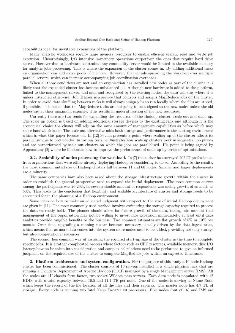
Scaling Beyond One Rack and Sizing of Hadoop Platform 425
capabilities ideal for inevitable expansions of the platform.
Many analytic workloads require large memory resources to enable efficient search, read and write jobexecution. Unsurprisingly, I/O intensive in-memory operations outperform the ones that require hard driveaccess. However due to hardware constraints any commodity server would be limited in the available memoryfor analytic jobs processing. This is where the expansion of the cluster comes in. By adding additional racksan organisation can add extra pools of memory. However, that entails spreading the workload over multipleparallel servers, which can increase accompanying job coordination overheads.
When all those conditions are met and an organisation has installed new nodes as part of the cluster it islikely that the expanded cluster has become unbalanced [4]. Although new hardware is added to the platform,linked to the management server, and seen and recognised by the existing nodes, the data will stay where it isunless instructed otherwise. Job Tracker is a service that controls and assigns MapReduce jobs on the cluster.In order to avoid data shuffling between racks it will always assign jobs to run locally where the files are stored,if possible. This means that the MapReduce tasks are not going to be assigned to the new nodes unless the oldnodes are at their maximum capacity. This results in underutilisation of the new resources.
Currently there are two tends for expanding the resources of the Hadoop cluster: scale out and scale up.The scale up option is based on adding additional storage devices to the existing rack and although it is theeconomical choice the cluster will rely on the same amount of management capabilities as before which maycause bandwidth issue. The scale out alternative adds both storage and performance to the existing environmentwhich is what this paper focuses on. In [12] Sevilla presents a point where scaling up of the cluster affects itsparallelism due to bottlenecks. In various tests he illustrates how scale up clusters work in sequential job phasesand are outperformed by scale out clusters on which the jobs are parallelised. His point is being argued byAppuswamy [2] where he illustrates how to improve the performance of scale up by series of optimisations.
2.2. Scalability of nodes processing the workload. In [7] the author has surveyed 202 IT professionalsfrom organisations that were either already deploying Hadoop or considering to do so. According to the results,the most common initial size of Hadoop clusters fall between 11 and 60 nodes. Smaller and larger deploymentsare a minority.
The same companies have also been asked about the storage infrastructure growth within the cluster inorder to establish the general prospective need to expand the initial deployment. The most common answeramong the participants was 20-29%, however a sizable amount of respondents was seeing growth of as much as50%. This leads to the conclusion that flexibility and scalable architecture of cluster and storage needs to beaccounted for in the planning of a Hadoop environment.
Some ideas on how to make an educated judgment with respect to the size of initial Hadoop deploymentare given in [11]. The most commonly used method involves estimating the storage capacity required to processthe data currently held. The planner should allow for future growth of the data, taking into account thatmanagement of the organisation may not be willing to invest into expansion immediately, at least until dataanalytics provide tangible benefits to the business. Two common estimates are flat growth of 5% or 10% permonth. Over time, upgrading a running cluster becomes necessary, usually driven by the data ingest rates,which means that as more data comes into the system more nodes need to be added, providing not only storagebut also computational resources.
The second, less common way of assessing the required start-up size of the cluster is the time to completespecific jobs. It is a rather complicated process where factors such as CPU resources, available memory, disk I/Olatency have to be taken into consideration and complex calculations need to be performed to give an informedjudgment on the required size of the cluster to complete MapReduce jobs within an expected timeframe.
3. Platform architecture and system configuration. For the purpose of this study a 16 node Hadoopcluster has been commissioned. The cluster consists of 16 servers installed in a single physical rack that arerunning a Cloudera Deployment of Apache Hadoop (CDH) managed by a single Management server (IMS). Allthe nodes are 1U chassis form factor, two socket Wildcat pass servers. Each data node is populated with 12HDDs with a total capacity between 10.5 and 11.4 TB per node. One of the nodes is serving as Name Nodewhich keeps the record of the file location of all the files and their replicas. The master node has 4.7 TB ofstorage. Every node is running two Intel Xeon E5-2697 v3 processors. Five nodes (out of 16) and IMS are

426 W. Litke and M. Budka
populated with 252.2 GB of RAM. The remaining nodes use 125.9 GB of memory. Connectivity is provided bythe 40 GbE.
The cluster is linked to an automated OS/configuration provisioning system. It is a mechanism that allowsautomatic deployment, monitoring, updating and management of all the nodes. It has been used to deploy theOS1.
In order to deploy Hadoop 2.0, Cloudera Manager version 5.3.3 has been utilised. Cloudera Manager is apiece of software that simplifies and shortens the process of Hadoop installation and configuration. The built-inmonitoring utilities have been used to collect data for this study.
4. TeraSort benchmark. Careful consideration has been put into the choice of benchmarks used tovalidate the outcomes of this study. Ultimately the TeraSort benchmark suite has been chosen as a singlepoint of reference. TeraSort is a set of benchmarks very widely known and used in the Hadoop world [9]. It’spurpose is to test the CPU power of the cluster. The benchmark conveniently has data generation utilities aswell as sorting functionality. It consists of three stages: teragen, terasort and teravalidate. The benchmarkingprocedure starts with teragen which generates a data set of size specified as the number of rows to be createdduring the run. Terasort uses Map and Reduce functions to sort the generated dataset, which is then read andvalidated by teravalidate.
For the purpose of this study two teragen sizes have been used: 10 bln (bln=billion) and 20 bln rows, inorder to accommodate benchmarking scalability.
Before the benchmark is run, the script performs a pre-run clean-up of the root directories to guarantee aclean run every time. Without that step the directories could be filled with data from previous benchmark runsand compromise the consistency of testing as the preconditions of the cluster would be different to the previousstep. In cases where a number of nodes had to be decommissioned (part 2 of testing) some manual cleaning ofdirectories was required.
After the clean-up is complete, the following sequence of tests is run three times:1. Teragen - 10 bln,2. Terasort - 10 bln,3. Teravalidate - 10 bln,4. Teragen - 20 bln,5. Terasort - 20 bln,6. Teravalidate - 20 bln,
producing a total of 18 test results per script run.The benchmark metrics can then be retrieved from Cloudera Manager (Yarn >Applications). Two main
metrics have been recorded:1. Time to complete, which marks the duration of the run for every benchmark, as the most meaningful
indication of the cluster performance.2. CPU time, which is the total time the processor has spent executing instructions during the run and is
usually expressed in higher time units e.g hours (h) or days (d). On multi-processor machines like theones in this study, where each CPU holds multiple cores, the total CPU time is calculated by summingup the CPU time for all processors and their cores. This metric gives an indication of the energyefficiency of a particular processing scenario.
The results for each run are collected and an average for every test from all three runs is taken, with aprovision that any deviation larger than 20% will call for a full retest, which is a protocol accepted at thecompany that has provided the facilities for this study.
Also to validate the acceptable range of results a 99% confidence interval for mean has been calculated [1],giving an indication of a tolerable margin of error in the results based on the sample size, observed mean andstandard deviation.
1For confidentiality reasons the name of the OS vendor has been withheld. List of OSs compatible with Cloudera can befound at: www.cloudera.com/content/cloudera/en/documentation/cdh4/latest/CDH4-Requirements-and-Supported-Versions/
cdhrsv topic 1.html

Scaling Beyond One Rack and Sizing of Hadoop Platform 427
5. Results.
5.1. Scaling beyond 1 rack. In the first part of the benchmarking process three tests have been performed(cf. Table 5.1). The mean of the three runs in all three tests have been used to examine the implications ofscaling out Hadoop beyond one rack.
Table 5.1: Scaling beyond one rack tests specification
Test no # of nodes Notes Label
1 16 deployed in 1 rack 16-node-A2 16 deployed in 2 logical racks, 8 nodes each 16-node-B3 8 deployed in 1 rack 8-node
Fig. 5.1(a) summarises the time to complete for tests 16-node-A, 16-node-B and 8-node. As it can be seenthe differences between 16-node-A and 16-node-B are marginal. A single rack with all 16 nodes performedslightly better when generating and handling 10 bln rows. As expected, the difference between the first two andthe third benchmark consisting of only 8 nodes is considerable - the benchmark took more than 2 times longerto complete in the latter case.
There is no surprise in that difference as the number of nodes has been halved. In case of teragen and terasort
the time to complete grew by 102% and 144% respectively. The teravalidate time however has surprisinglyincreased by as much as 265% relative to 16-node-B test results.
The results from generating 20 bln rows prove to differ from the 10 bln row scenario. As it can be seen inFig. 5.1(a) the results from 16-node-A and 16-node-B appear to be very similar. While in test 16-node-A thetime to complete on teragen is considerably lower than test 16-node-B, in the case of terasort and teravalidate
it’s only marginally shorter.Similarly to 10 bln row benchmarking the differences in results on 20 bln rows between tests 16-node-A
and 16-node-B remain very small. In fact, they are small enough to say that they fall within the margin oferror (cf. Fig. 5.1(b)). A t-test, which according to [1], T-test takes into account all the three results from thebenchmarking and can judge whether the difference between the two data sets is statistically significant. Thetest compared the result of all three runs between both tests A and B revealed, that in the case of terasort andteravalidate the differences in results are not statistically significant .
Results from the 8-node test show that the cluster has taken 106%, 138% and 347% longer to completeteragen, terasort and teravalidate respectively.
The CPU time metric does not show major changes between the benchmarks results. For both the 10 and20 bln scenario, the results are very close to each other as depicted in Figs. 5.1(c) and 5.1(d).
5.2. Scalability of Hadoop cluster. The second part of testing constitutes of a series of tests that aimto evaluate performance difference when choosing to deploy clusters of varying sizes. The specification of thetest has been given in Table 5.2.
Table 5.2: Scalability of Hadoop cluster tests specification2
Test no # of nodes Label
1 16 16-node test4 14 14-node test5 12 12-node test6 10 10-node test3 8 8-node test
2The results from test 1 and 3 have been reused as the their specifications matched the required testing. The test numbering infirst column is dictated by the number of nodes in the tested cluster.
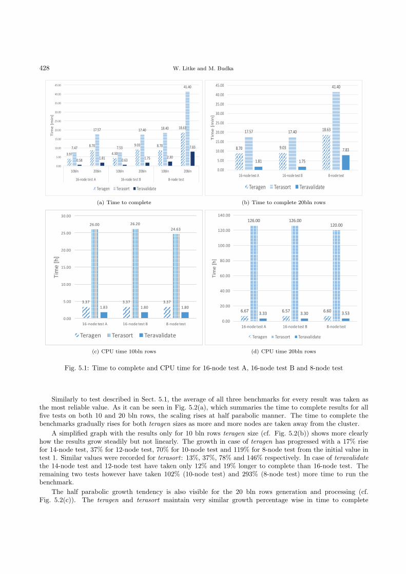
428 W. Litke and M. Budka
!"#$
%"$&
'"!&
#"&! %"$&
(%")!
$"'$
($"*$
$"*!
($"'& (%"'&
'("'&
&"*%("%(
&")!("$* +"!&
$"%!
&"&&
*"&&
(&"&&
(*"&&
+&"&&
+*"&&
!&"&&
!*"&&
'&"&&
'*"&&
(&,-. +&,-. (&,-. +&,-. (&,-. +&,-.
()/.0123425436 ()/.0123425437 %/.01234254
89:23;:9.<
82=>?2. 82=>50=4 82=>@>-91>42
(a) Time to complete
!"#$ %"$&
'!"(&'#")# '#"*$
*'"*$
'"!' '"#)
#"!&
$"$$
)"$$
'$"$$
')"$$
+$"$$
+)"$$
&$"$$
&)"$$
*$"$$
*)"$$
'(,-./01203214 '(,-./01203215 !,-./012032
67801987-:
60;<=0- 60;<3.;2 60;<><?7/<20
(b) Time to complete 20bln rows
!"!# !"!# !"!#
$%"&& $%"$&
$'"%!
(")! (")& (")&
&"&&
*"&&
(&"&&
(*"&&
$&"&&
$*"&&
!&"&&
(%+,-./01/2103 (%+,-./01/2104 )+,-./01/21
567/089:
5/;<=/, 5/;<2-;1 5/;<><?6.<1/
(c) CPU time 10bln rows
!"!# !"$# !"!%
&'!"%% &'!"%%&'%"%%
("(( ("(% ("$(
%"%%
'%"%%
)%"%%
!%"%%
*%"%%
&%%"%%
&'%"%%
&)%"%%
&!+,-./01/2103 &!+,-./01/2104 *+,-./01/21
567/089:
5/;<=/, 5/;<2-;1 5/;<><?6.<1/
(d) CPU time 20bln rows
Fig. 5.1: Time to complete and CPU time for 16-node test A, 16-node test B and 8-node test
Similarly to test described in Sect. 5.1, the average of all three benchmarks for every result was taken asthe most reliable value. As it can be seen in Fig. 5.2(a), which summaries the time to complete results for allfive tests on both 10 and 20 bln rows, the scaling rises at half parabolic manner. The time to complete thebenchmarks gradually rises for both teragen sizes as more and more nodes are taken away from the cluster.
A simplified graph with the results only for 10 bln rows teragen size (cf. Fig. 5.2(b)) shows more clearlyhow the results grow steadily but not linearly. The growth in case of teragen has progressed with a 17% risefor 14-node test, 37% for 12-node test, 70% for 10-node test and 119% for 8-node test from the initial value intest 1. Similar values were recorded for terasort : 13%, 37%, 78% and 146% respectively. In case of teravalidatethe 14-node test and 12-node test have taken only 12% and 19% longer to complete than 16-node test. Theremaining two tests however have taken 102% (10-node test) and 293% (8-node test) more time to run thebenchmark.
The half parabolic growth tendency is also visible for the 20 bln rows generation and processing (cf.Fig. 5.2(c)). The teragen and terasort maintain very similar growth percentage wise in time to complete

Scaling Beyond One Rack and Sizing of Hadoop Platform 429
!"#$
%"$&
'"(!
#")!
)"'!
**"'!
("$!
*'"&!
%"$&
*%"(!
$"'$
*$")$
%"'!
+&"+$
*&"+!
+'")&
*!"!&
!&"%!
*%"'&
'*"'&
&")%*"%*
&"()+"($
&"(#
!"*!*"*$
'"(&+"!&
$"%!
&"&&
)"&&
*&"&&
*)"&&
+&"&&
+)"&&
!&"&&
!)"&&
'&"&&
')"&&
*&,-. +&,-. *&,-. +&,-. *&,-. +&,-. *&,-. +&,-. *&,-. +&,-.
*(/.01234254 *'/.01234254 *+/.01234254 *&/.01234254 %/.01234254
67823987.:
62;<=2. 62;<50;4 62;<><-71<42
(a) Time to complete
!"#$%"&!
'"%!
&"$!
("$)
$"%$("%!
*)"+!
*!"!)
*("%)
)"'( )"&' )"&#*"*$
+"!)
)"))
+"))
%"))
&"))
("))
*)"))
*+"))
*%"))
*&"))
*("))
+)"))
*&,-./01 *%,-./01 *+,-./01 *),-./01 (,-./01
2340,543-6
207890- 20781.7: 2078;8<3/8:0
(b) Time to complete 10bln rows
!"#$ %"&'((")'
()"$'
(!"*'(#"&#
+$"+#
+)"&$
'$"!'
)(")$
("!( +"*# '"(')"*$
#"!'
$"$$
&"$$
($"$$
(&"$$
+$"$$
+&"$$
'$"$$
'&"$$
)$"$$
)&"$$
(*,-./01 (),-./01 (+,-./01 ($,-./01 !,-./01
2340,543-6
207890- 20781.7: 2078;8<3/8:0
(c) Time to complete 20bln rows
!"!# !"!# !"$% !"&# !"!#
'&"%% '&"(# '&"%!'&")!
'*"&!
("+! ("+( ("+* ("++ ("+%
%"%%
$"%%
(%"%%
($"%%
'%"%%
'$"%%
!%"%%
(&,-./01 (*,-./01 (',-./01 (%,-./01 +,-./01
2340,543-6
207890- 20781.7: 2078;8<3/8:0
(d) CPU time 10bln rows
!"!# !"#$ #"%$ #"&$ !"!%
'(!"%% '(!"%%'$%"%% '$("%%
'(%"%%
$"$$ $"&% $")# $"#% $")$
%"%%
(%"%%
&%"%%
!%"%%
*%"%%
'%%"%%
'(%"%%
'&%"%%
'!+,-./0 '&+,-./0 '(+,-./0 '%+,-./0 *+,-./0
123/+432,5
1/678/, 1/670-69 1/67:7;2.79/
(e) CPU time 20bln rows
Fig. 5.2: Time to complete and CPU time for 16, 14, 12, 10 and 8 nodes

430 W. Litke and M. Budka
compared to the results of 10 bln tests. The changes in the teravalidate benchmark are more dramatic with48% growth in 14-node test, 72% in 12-node test, 154% in 10-node test and 333% in 8-node test compared to16-node test.
Similarly to the experiments of Sect. 5.2 the CPU time did not exhibit major fluctuations (cf. Figs. 5.2(d)and 5.2(e)).
During the tests we have also observed that the cluster CPU utilisation3 was gradually dropping as thesubsequent nodes were taken away to process the workload. In the 16-node test peaks were fluctuating aroundthe 55% mark, with a maximum of 56.57% as shown in Fig. 5.3(a).
In the 14-node test, with just two nodes less that number came down to about 45% with a peak at 46.82%(cf. Fig. 5.3(b)).
The cluster with another 2 nodes removed in 12-node test (cf. Fig. 5.3(c)) brought down the CPU utilisationto about 40% (peak at 40.78%).
In test 6 with 10 nodes the cluster CPU utilisation drops to about 30% reaching up to 32.61% at its highest(cf. Fig. 5.3(d)).
In the 8 node test (cf. Fig. 5.3(e)) the CPU utilisation stays just above 20% with peak utilisation of 23.25%.Throughout the testing we have kept a close eye on the Disk Latency of the drives on the utilised cluster.
Disk latency constitutes the amount of time that the hard drive takes to write a chunk of data. It has transpiredthat there are some serious constraints on the existing system. The lower the number of nodes processing theworkload, the higher the latency of the drives. In 16-node test the nodes were scoring a latency of up to 3.4seconds which is still a relatively high waiting time. However, as the tests progressed the bottleneck of drivelatency was becoming more apparent. The latency in 14-node test reached 12 seconds at its highest, in 12-nodeand 10-node tests - about 18 seconds and as much as 57 seconds in the last test on 8 nodes (cf. Fig. 5.3).
6. Analysis and discussion.
6.1. Scaling beyond one rack. Running the terasort benchmark on the cluster has shown that there isno major difference between the results on a single cluster deploying 16 nodes and two clusters with 8 nodeseach. While it would be intuitive to assume that it would consume some overhead to communicate between theracks, it appears that if properly installed and configured the split racks do not make a large difference.
In the case of this study, the first stage of benchmarking - teragen - generates the data on both clusterssimultaneously and it is distributed evenly. This is due to the design of Job Tracker, which is a built-in servicein Hadoop that oversees and manages the MapReduce jobs on the platform. It consults the Name Node to findout which Data nodes hold the necessary files to process a task. Job Tracker will always attempt to fetch thedata from a local node from the same rack. Only when that is not possible the Name Node will refer it outsideof the rack, reducing the overheads as a result.
A situation where this might prove not to be true is a cluster that is not balanced. ‘Balanced cluster’ is aterm describing a situation where the data is evenly distributed across all nodes in all the racks. In a situationwhere a company has a successfully running cluster to which they add an additional rack in order to expandtheir Hadoop platform, they end up unbalancing the system. The data stays on the old rack and the new oneremains empty. This often results in underutilisation of HDFS as the MapReduce tasks are not going to bescheduled on the added nodes unless the pre-existing racks are too busy to take new jobs. Also, the platformwill experience larger network bandwidth consumption and slower job completions. In cases where the newnodes are assigned MapReduce tasks that they do not have data to complete, the files will have to be carriedacross the network, ultimately negatively impacting the performance.
In case of the two racks used for our testing, all the data has been generated on both racks evenly and weknow that the cluster is balanced. The test results have proven that a Hadoop cluster if correctly designed doesnot lose on the performance when configured into more than one rack.
The testing also revealed that if we halved the amount of nodes processing the workload, the time to completehave increased by more than 100% on all three benchmarks while running both teragen sizes. Intuitively, theperformance drop should stay just short of 100% as we are reducing the amount of nodes by half and thereshould be some loss of performance due to overheads for split rack.
3Overall utilization of all CPUs in the whole cluster

Scaling Beyond One Rack and Sizing of Hadoop Platform 431
Time [min]0 30 60 90 120
CP
U lo
ad
[%
]
0
10
20
30
40
50
60
(a) 16-node test
Time [min]0 30 60 90 120
CP
U lo
ad
[%
]
0
5
10
15
20
25
30
35
40
45
50
(b) 14-node test
Time [min]0 30 60 90 120 150
CP
U lo
ad
[%
]
0
5
10
15
20
25
30
35
40
45
(c) 12-node test

432 W. Litke and M. Budka
Time [min]0 30 60 90 120 150 180 210
CP
U lo
ad
[%
]
0
5
10
15
20
25
30
35
(d) 10-node test
Time [min]0 30 60 90 120 150 180 210 240 270 300
CP
U lo
ad
[%
]
0
5
10
15
20
25
(e) 8-node test
Fig. 5.3: Cluster CPU utilisation
The marginal difference in the results between tests 16-node-A and 16-node-B have proven that the over-heads on a split rack are practically non-existent and the communication between the racks has a very minimalimpact on the performance. That however does not explain the over 100% increase in time to complete.
The explanation of the drastic performance difference lies with the inodes (or index nodes). Inode in a Unix-style files system is a data structure that keeps the contents of the file separate from the information storedabout the file. So for every file on the system there is a corresponding inode with a unique inode number [8].
Running close to the limit of inodes explains the excessive time to complete not only on the smaller clusterin 8-node test but also explains why duration of benchmarks more than doubles for 10 bln rows and 20 blnrows. The amount of inodes and the space reserved for them is set during the creation of the file system. Ifthere are a lot of small files created on the disk, like in our case during testing, the system starts to run outof inodes and drastically slows down long before it runs out of storage. This unfortunately cannot be changeddynamically without re-formatting the drives. If the drives run out of inodes, no more files can be created onthe drives. This is why it is critical to accommodate for enough inodes to successfully complete the workloadanalysis.

Scaling Beyond One Rack and Sizing of Hadoop Platform 433
6.2. Scalability of Hadoop cluster. During the benchmarking of the Hadoop cluster we have observeda gradual rise in time to complete on all three elements of the terasort benchmark. As the amount of nodesdrops, the time the platform requires to complete the process rises in a regular and predictable manner.
Also the analysis of the Cluster CPU activity clearly tells us that the smaller the node count the less theprocessor capacity is utilised. With the highest number of nodes in our test - 16 - we only managed to use justover half of the cluster CPU potential. By halving the amount of nodes we are only using as little as 20% oftotal capacity. The 150% increase in utilization in case of 16 node cluster compared to 8 is dictated by theincreased seek time on hard drives. Because the benchmarks are taking longer to complete, the stress on CPUis decreases as shown on figure 5.3, ultimately leading to underutilisation.
That activity very closely links to the Disk Latency already mentioned in Sect. 5.2, a hard drive consists ofmoving mechanical parts, some of the more important ones include platter, where the data is written, spindlethat spins the platter, heads which write and read the data to/from the platter and is attached to the armthat moves the head to the right spot on the platter. Inodes can be treated as logical cells that have a spaceassigned on the platter. Those spaces are allocated during hard drive formatting and cannot be altered. As thehead writes the data to the platter, the inodes become assigned to each file on the drive. When there is a largeamount of small files created on the drive the inodes run out and the system cannot save any more data. Asthe drive exhausts the inodes available, the seek time to write the data is extending. It takes more and moretime to find a free inode and only then a file can be assigned to it (written). We can see that clearly in Fig. 6.1.
According to Microsoft and Oracle an acceptable disk latency in the industry should not exceed 10 ms [6].In the best case scenario on a 16 node cluster we are experiencing as much as 3 seconds of latency on the disks.It exceeds the industry desired standards three hundred times. In comparison, for the 8 node cluster the latencyis up to 57 seconds. It is clear that is a major cause of bottlenecks.
7. Conclusions and future work. In this paper we have explored two case scenarios where the hardwareconfiguration plays a large role in the performance of the cluster and will have an impact on the Big Dataanalytics workloads. In the first part we have established that as long as the data is evenly balanced acrossall the racks that make up the Hadoop platform, there are minimal overheads to accommodate the split racks.The corporations that decide to expand their Big Data environment have to remember to make use of balancingutilities to achieve that goal – otherwise the result will not reflect our findings.
During the testing process it transpired that the disk latency may cause high impact constraints. Theseconstraints negatively impacted the duration of testing as well as utilisation of resources. In some cases wehave experienced in excess of 200% or 300% increase in time required to complete benchmarks where we wereexpecting about 100% as we were either doubling the workload or halving the amount of resources. What wealso have to keep in mind is that the testing conducted was a relatively small scale compared to what some largescale corporations deploy; their workloads also are considerably larger than the terasort benchmark. The harddrive seek time delays in those larger deployments may cause even bigger gap between the expected performanceand what they actually achieve.
We have also found that the more the system is required to focus on seeking the inodes on the drives,the less it focusses on processing the workload. This, combined with lower amount of nodes, ultimately leadsto lower cluster CPU utilization. It is a large financial commitment for an origination to invest in hardware,especially enterprise class hardware. It is in their best interest to make sure that those resources are used tothe best of their capabilities. That is why it is important that the corporation accurately assess the size andpurpose of the Hadoop platform in order to correctly choose the required size of the cluster and also invest timeto optimally configure it and test for bottlenecks.
There is yet a lot to explore in the domain of Hadoop optimisation. Although we have investigated theimplications of different deployment scenarios and have found answers to our questions we also have found thatthe CPU time on the smallest 8-node cluster was shorter than on the larger ones. As the focus of this study wasbiased more towards the duration of the benchmarking, this issue has not been given much attention. Futureanalysis of the problem from the CPU side might give us more insight into other potential bottlenecks. Alsothe benchmarking on larger scale clusters with more variety of benchmark suites may unveil larger performancegap in the duration of the benchmarking as well as the CPU time.
Furthermore, in the light of current emphasis on the environmental footprint caused by the datacentres

434 W. Litke and M. Budka
Time [min]0 20 40 60 80 100 120
La
ten
cy [m
s]
0
500
1000
1500
2000
2500
3000
3500
(a) 16-node test
Time [min]0 20 40 60 80 100 120 140 160
La
ten
cy [m
s]
0
2000
4000
6000
8000
10000
12000
14000
16000
18000
20000
(b) 12-node test
Time [min]
0 50 100 150 200 250 300
La
ten
cy [s]
0
10
20
30
40
50
60
Fig. 6.1: Maximum disk latency

Scaling Beyond One Rack and Sizing of Hadoop Platform 435
we would like to explore the power consumption dependence on various factors such as deployment model,configuration or number of nodes.
Also the investigation of networking choices and their impact would link to this study as the performancemay be affected by the connectivity choices on the platform. Hence we plan to look into upgrading the clusterto InfiniBand in the future and present the difference in performance.
Acknowledgements. We gratefully acknowledge the support from of Mr. S. G. Anderson, Big DataSolutions Engineer who has enabled the benchmarking process to take place at the Cloud and Big Data lab ofthe Client.
REFERENCES
[1] D. Altman, D. Machin, T. Bryant, and M. Gardner, Statistics with confidence: confidence intervals and statisticalguidelines, John Wiley & Sons, 2006
[2] R. Appuswamy, C. Gkantsidis, D. Narayanan, O. Hodson and A. Rowstron, Scale-up vs scale-out for Hadoop: time torethink?, Proceeding SOCC ’13 Proceedings of the 4th annual Symposium on Cloud Computing Article No. 20, 2013.
[3] J. Dean, S. Ghemawat, MapReduce: Simplified Data Processing on Large Clusters, Communications of the ACM - 50thanniversary issue 51 (1), 2008, pp. 107-113
[4] B. Hedlund, Understanding Hadoop Clusters and the Network, tech. report, 2011, http://bradhedlund.com/2011/09/10/understanding-hadoop-clusters-and-the-network
[5] Hortonworks, Cluster Planning Guide, tech. report, 2013, http://docs.hortonworks.com/HDPDocuments/HDP1/HDP-1.3.0/bk cluster-planning-guide/bk cluster-planning-guide-20130528.pdf
[6] E. Markovich, Whats An Acceptable I/O Latency?, tech. report, Kaminario, 2010, http://kaminario.com/blog/whats-an-acceptable-io-latency/
[7] A. Nadkarni, Trends in Enterprise Hadoop Deployments, tech. report, IDC, 2013, http://www.avnetweb.com/comms/avnet/redhat/liberate/resources/Trends in Enterprise Hadoop Deployments.pdf
[8] E. Nemeth, UNIX and Linux system administration handbook, Pearson Education, 2011.[9] M. G. Noll, Benchmarking and Stress Testing an Hadoop Cluster With TeraSort, TestDFSIO & Co., 2011,
http://www.michael-noll.com/blog/2011/04/09/benchmarking-and-stress-testing-an-hadoop-cluster-with-terasort-testdfsio-nnbench-mrbench
[10] N. Rouda, Achieving Flexible Scalability of Hadoop to Meet Enterprise Workload Requirements, tech. report, EnterpriseStrategy Group, 2014, http://www.emc.com/collateral/analyst-reports/esg-emc-achieving-flexible-scaling-hadoop.pdf
[11] E. Sammer, Hadoop operations, O’Reilly Media, Inc., 2012.[12] M. Sevilla, I. Nassi, K. Ioannidou, S. Brandt and C. Maltzahn, A framework for an in-depth comparison of scale-up and
scale-out, DISCS-2013 Proceedings of the 2013 International Workshop on Data-Intensive Scalable Computing Systems,pp. 13-18
[13] M. E. Wendt, Cloud-based Hadoop Deployments: Benefits and Considerations, tech. report, Accenture Technology Labs,2014. https://www.accenture.com/t00010101T000000 w /jp-ja/ acnmedia/Accenture/Conversion-Assets/DotCom/Documents/Local/ja-jp/PDF 2/Accenture-Cloud-Based-Hadoop-Deployments-Benefits-and-Considerations.pdf
[14] T. White, Hadoop: The definitive guide, O’Reilly Media, Inc., 2012.[15] C. Wilson, Who’s Using Hadoop and What are They Using It For?, 2015, http://blog.syncsort.com/2015/06/whos-using-
hadoop-and-what-are-they-using-it-for
Edited by: Dana PetcuReceived: July 10, 2015Accepted: September 30, 2015


Scalable Computing: Practice and Experience
Volume 16, Number 4, pp. 437–448. http://www.scpe.org
DOI 10.12694/scpe.v16i4.1132ISSN 1895-1767c⃝ 2015 SCPE
ENERGY EFFICIENCY OF PARALLEL MULTICORE PROGRAMS
DAVOR DAVIDOVIC∗, MATJAZ DEPOLLI†, TOMISLAV LIPIC∗, KAROLJ SKALA∗, AND ROMAN TROBEC†
Abstract. The increasing energy consumption of large-scale high performance resources raises technical and economicalconcerns. A reduction of consumed energy in multicore systems is possible to some extent with an optimized usage of computingand memory resources that is tailored to specific HPC applications. The essential step towards more sustainable consumption ofenergy is its reliable measurements for each component of the system and selection of optimally configured resources for specificapplications. This paper briefly surveys the current approaches for measuring and profiling power consumption in large scalesystems. Then, a practical case study of a real-time power measurement of multicore computing system is presented on two realHPC applications: maximum clique algorithm and numerical weather prediction model. We assume that the computing resourcesare allocated in a HPC cloud on a pay-per-use basis. The measurements demonstrate that the minimal energy is consumed whenall available cores (up to the scaling limit for a particular application) are used on their maximal frequencies and with threadsbinded to the cores.
Key words: Energy efficiency, high-performance, maximum clique, numerical weather prediction
AMS subject classifications. 65Y05, 68U20
1. Introduction. Nowadays, a large number of hard problems is being solved efficiently on large-scalecomputing systems such as clusters, grids and clouds. The main building blocks of such systems are high-performance computing (HPC) clusters, since they are furthermore embedded both into grid computing systemsas well as cloud computing systems [1]. A great advantage of Graphical Processor Unit (GPU) accelerators overmulticore platforms was demonstrated in terms of energy efficiency [2] with an overall energy consumption foran order of magnitude smaller for the GPUs. Inside the clusters, the many-core architectures, such as GPUs [3],as well as even more specialized data-flow computers [4] are getting an increasingly large supporting role butthe main processing is still performed by the multi-core main processors because of simple programming model.In this research, we analyze the energy consumption profile of the processors on a two processor multi-corecomputer, while varying its workload.
With the increasing number of components in large-scale computing systems the energy consumption issteeply increasing [5]. In computer systems, energy (measured in Joules) is represented as the electricity resourcethat can power the hardware components to do computation. On the other hand, power is the amount of energyconsumed per unit time (measured in Joules per second or Watts). The ever-increasing energy consumption oflarge-scale computing systems causes higher operation costs (e.g. electricity bills) and has negative environmentalimpacts (e.g. carbon dioxide emissions). Therefore, when designing large-scale computing systems, the focus isoften shifting from performance improvements to energy efficiency.
Energy can be reduced at several levels of the distributed architecture: individually on each node or hardwarecomponent-level, at the middleware level, at the networking level, and at the application level [6, 7, 8, 9].
Suboptimal use of systems resources (e.g. over-provisioning) is the primary source of energy inefficiency atmiddleware layer [6, 7, 10]. In over-provisioned systems, components usually consume excessive power whenthey are relatively idle or underutilized. This is important from the user point of view, because pay-per-use approaches stimulate users to maximally exploit rented resources during the execution period. Energy-proportional computing [11] introduces the concept of consuming energy proportional to resource utilization sothat an idle or underutilized component consumes less energy. For improving the energy efficiency at middlewarelayer, energy-aware resource and workload management algorithms are utilized [10]. Increased network traffic inmany bandwidth sensitive network applications results also in increased number of networking devices such asswitches and routers and therefore in increased energy consumption. Thus, different approaches for new energyaware network protocols and network infrastructure, e.g., software defined networks and network functionsvirtualization, are developed also for improving energy efficiency at network layer [12, 13].
∗Rudjer Boskovic Institute, Centre for Informatics and Computing, Zagreb, Croatia†Jozef Stefan Institute, Department of Communication Systems, Ljubljana, Slovenia
437

438 D. Davidovic, M. Depolli, T. Lipic, K. Skala and R. Trobec
A processor is a component that dominates the energy consumption of each node. Thus, most of techniquesare designed to reduce energy consumption of the processor [14, 15, 16]. Most of the current processors areimplemented with dynamic voltage and frequency scaling regulators to optimally adjust the voltage/frequency atrun-time according to the workload behavior. Paper [17] focuses on the dynamic control of the voltage regulatorsin a chip multicore processors platform. Results from detailed simulations based on realistic experimental setupsdemonstrate up to 9% total energy saving. In [18] a minimum energy voltage scheduling on a single multi-core processor with software controlled dynamic voltage scaling is proposed. Another hardware approach forimproving power management for multi-core systems is with implementation of multiple voltage islands [19].Different frequency scaling schemes were investigated in the past that minimize the total energy consumption.The problem is even more critical in the real-time applications scheduling with pre-specified tasks’ deadlines [20].
The energy consumption heavily depends on the characteristic of applications. Some applications are com-putationally intensive, other are data intensive, while other are hybrid of both. Energy-aware programmingmodels, regarding various types of workloads and architectures, are required to develop energy efficient appli-cations [21, 22]. Programming approaches, based on optimal utilization of shared hardware on-chip resources,e.g. cache memory, memory bandwidth, threads or cores, for improved energy efficiency are becoming popularbecause of their simple implementation. In heterogeneous multicore processors that integrate CPU cores anddata-parallel accelerators (GPU) last-level cache memory can be managed to minimize the energy consump-tion [23]. The dynamic assignment of thread-to-core can be particularly beneficial in saving the energy [24, 25].
These approaches are particularly important in the case of modern multi-core building blocks that have alot of options for controlling the execution parameters, e.g., number of cores, system frequency, core binding,etc. The energy can be thus saved at all levels of large-scale architectures, even dynamically, depending on theapplication program characteristics.
In this research we experimentally test the effects of the workload, core binding strategies, and frequencyscaling on energy requirements for two existing applications. We build on the previous research [26] withaddition of a communication intensive use case that significantly influences energy consumption. Our approachdoes not require any change in the original source code of the applications and is thus instantly applicableon a wide range of applications without inspecting their code. Our findings suggest that modern multi-corearchitectures perform best both energy-wise and performance-wise when all of the cores are used, the frequencyis not throttled and threads are not allowed to migrate between cores.
The paper starts with a brief survey of the current approaches for measuring and profiling power consump-tion in Sect. 2. In Sect. 3, two different use cases are presented together with the description of the experimentalcomputer for software-based energy measurements. In Sect. 4, the obtained results are shown under various testconditions, which demonstrate significant differences in the consumed energy. The results are discussed in moredetails in Sect. 5 in order to deduce some useful rules for users of HPC cloud resources. The paper concludeswith the summary of results and directions for further work.
2. Energy Measurement and Profiling Approaches. The essential step towards the energy-efficiencyis accurate, reliable and continuous energy consumption measurement of the system components. Energymeasurement and profiling approaches can be classified as hardware-based, software-based and hybrid. In thefollowing subsections the basic characteristics of hardware-based and software-based approaches are outlined,based on two extensive survey papers [27, 28].
2.1. Hardware-based Energy Measurement. Hardware-based energy measurement approaches areimplemented with various instruments or sensors that measure the electrical current or the consumed energyas functions of time on different computation, storage or networking segments such as CPUs, motherboards,servers or racks. An energy measurement obtained with meters is a direct and straight-forward approach. Adigital multi-meter collects the voltage or the energy samples of the measured segment in pre-specified timeintervals and sends the measurements through a data link connected to the data collection system. Such metersare mainly used to measure the direct current (DC) power and are connected between the power supply andthe measured segment. On the other hand, there are other meters (e.g. “Watts UP“ [29]) that can directlymeasure the power consumption on the alternating current (AC) lines. Another example of a simple meter withlimited precision is a clamp meter that has a larger measurement range and can be used to measure the energyof segments with high currents. AC meters, however, only measure the power consumption on the system level.

Energy Efficiency of Parallel Multicore Programs 439
In their simplicity, multi-meters cannot be used when a higher control of the measurement process isrequired. In those cases, more complex devices have to be used that are often custom designed. In 2000, Viredazet al. designed a platform called Itsy to measure the energy consumption of mobile devices [30]. Another exampleof a complex device to measure the energy consumption is a single board on computer called PLEB [31]. PLEBuses a design with a set of on-board current sensors, and an analogue-to-digital converter with a micro-controllerto read the sensors. Unlike Itsy, which measures only the energy consumption of mobile devices, PLEB canbe used to measure the energy of processors, memories, flash drivers, and I/O components. Precise and fine-grained measuring is also available through PowerPack, a system for power profiling on typical clusters or otherdistributed systems [32]. PowerPack measures power on system DC power lines and then maps it to individualcomponents of the system, using computer models. It also measures AC power consumption to derive theefficiency of AC to DC conversion. All measurement are processed on a separate computer to ensure the powerprofiling does not impact the system under test. PowerPack profiling is enabled by the provided API calls, thatlink the application under test to control and communicate with the meter control process and thus correlatethe power profiles with the application source code. Since PowerPack uses both hardware- and software-basedmethods of measurements it is actually a hybrid meter.
2.2. Software-based Energy Measurement. The disadvantages of hardware-based energy measure-ment techniques are in their dependence on the expensive sensing components and complex additional hardwaredesign. Considering the expensive and cumbersome setup, they are also not well suited for online monitoringand designing of energy-aware policies. In contrary, software-based approaches can be used to supply morefine-grained online information, although with reduced accuracy. They are more flexible because they can beapplied to different platforms without changing the hardware.
A software-based approach usually builds power/energy models to estimate the energy consumption at theCPU instruction level, program block level, process level, hardware component level or full system level. Thesemodels are built based on selection and optimization of power/energy indicators of a software or a hardwarecomponent of interests. Regarding the power/energy indicators type, software based approaches can be classifiedas system profile-based approaches or hardware performance counter (PMC) based approaches.
System profile or system events are a set of performance statistical information supplied by the operatingsystem or a special software. These events can describe the current state of hardware, software, and operatingsystem. For example, Joulemeter [33], tracks the energy consumption of a virtual machine using power/energymodels for three system hardware components, i.e. CPU, memory and disk. The CPU energy model uses CPUutilization, the memory energy model uses the number of last level cache misses, while the disk energy modeluses the bytes of data written to and read from the disk as inputs to their energy consumption estimates.
Hardware performance counters are a group of special registers that count the hardware-related activitieswithin the computer systems. The PMC-based modelling [34] is implemented either with top-down or bottom-upapproaches. The first do not depend on modelled architecture thus enabling a fast and an easy deployment [35],while the second depends on the underlying architecture and is therefore able to produce more informative,responsive and accurate power/energy models. The bottom-up approach enables a breakdown of the energyconsumption per architectural components, but is more complex to deploy and less portable than the simplertop-down approach [36].
3. Use Cases and Experimental Setup. The use cases, presented in this section, have been used astest applications for the analyses of energy consumption using real-time power monitoring. The experimentalcomputer comprised multi-core components, which are the main building blocks of the contemporary large-scale computing systems, including those offered by the cloud infrastructure providers. The two use cases areof different types based on their scalability characteristics. The first is characterized by high scalability on themulti-core computer systems, and second is characterized by high communication costs, which limit the scala-bility. The use cases are also implemented with different parallelization techniques, master-slave parallelizationand domain decomposition, and are consequently not equally sensitive to the computer architecture details,such as the amount of cache memory and the number of its levels.
Under the assumption that energy consumption scales linearly with the problem size on the selected usecases, we chose to experiment on small problems. With this assumption, the obtained results should also berepresentative for the larger problems.

440 D. Davidovic, M. Depolli, T. Lipic, K. Skala and R. Trobec
3.1. Maximum Clique Algorithm. For the first use case, we use an application that implements theparallel maximum clique algorithm [37], which is essentially a recursive program for traversing in a searchtree under the branch and bound strategy. The algorithm takes an input graph and returns its maximal fullyconnected sub-graph. The maximum clique algorithm is characterized as a compute-bound algorithm and willthus benefit if more processing units are employed for its solution. It is parallelized by using threads for searchingthe tree branches asynchronously. The threads are synchronized only when accessing one global variable - thesize of the current clique. On large graphs - these are graphs that take at least a few seconds to search through- the algorithm experiences a near-linear speedup on average.
As in all branch and bound approaches, the order in which the branches are searched influences the timerequired to find the optimal solution. In general, the concurrent search of several branches influences on whichbranches are searched and which not, which results in varying efficiency of the approach when used on variousnumber of threads. The effects of parallel speedup, which influences the energy consumption greatly, can thusbe hidden in the noise, generated by the varying branch and bound efficiency, which could make this algorithmtricky to evaluate.
For our experiments, a small graph named p hat300-3 from the DIMACS collection of benchmark graphsfor the maximum clique problem [38] was used. This graph comprises 300 vertices and 33390 edges, while itsmaximum clique spans over 36 of its vertices. The time required to find the maximum clique of p hat300-3 ona single core of the experimental computer setup is about 1.3 seconds. A quality of this graph when searchedby the selected maximum clique algorithm is also that it experiences relatively smooth speedup with almostconstant branch and bound efficiency across the range of the experimented number of cores. By using thisgraph, we streamline the experiments that would otherwise have to be made on a large set of input graphs justto cover the average algorithm speedup.
3.2. WRF meteorological model. The second use case is a public domain Weather Research and Fore-casting model (WRF-ARW) [39, 40]. This is a next-generation numerical weather prediction system designed toserve both operational forecasting and atmospheric research needs. The model, based on the input parametersand data, gives as an output a prediction of several atmospheric phenomena such as temperature, moisture,wind speed and direction, and precipitations. The model operates on a target geographical domain that isdivided into a grid. The distance between the grid points is called resolution. To increase the accuracy ofthe forecast for a specific region, a smaller nested domain is defined within the main domain. The forecast isconducted at each grid point on multiple vertical levels (3D grid) for each time step.
In the experiments we compute a 6-hour weather forecast for Croatia with one nested domain. The maindomain consists of 100 × 68 points and the nested domain of 58 × 61 points with 18 and 6 km resolution,respectively, and 27 vertical levels. The time step is 2 minutes for the main, and 40 seconds for the nesteddomain, thus, the number of iterations/steps is 180 and 1080 for the main and nested domain, respectively. Thetotal number of performed steps, for the 6-hour simulation, is 1.36× 10⁸.
The model applies different model for parallelism: MPI, OpenMP and hybrid MPI+OpenMP, that enableexecution on various computing architectures such as distributed and shared-memory (SMP) systems, clusters ofSMPs, and vector and multiprocessors base systems. The parallelism in the model is achieved by decompositionof geographical domain (a domain on which the model simulation is run) into a 2D grid. The grid consistsof patches, the rectangular sections of the model domain, each one allocated to a distributed memory nodeand executed by one MPI process. On a node level, each patch is further divided into tiles, which are thesquare sections of a patch, allocated to a shared-memory processor and each tile is executed by a single thread(i.e. OpenMP thread). Since our testing system is a shared-memory multi-core machine, only the OpenMPparallel version was considered. Thus, the domain is decomposed into 1 patch and the number of tiles equalsto the number of threads (in our case up to 12 threads). The tiles are processed concurrently by differentthreads, but, if the tile size cannot fit into the CPU’s cache memory, an additional communicational overheadis exhibited.
In contrast to the maximum clique algorithm, the performance of WRF is significantly leveraged by thecommunication and data exchange between the tiles that limit the scalability of the model and is thus concernedas a memory-bound algorithm.

Energy Efficiency of Parallel Multicore Programs 441
3.3. Experimental Setup. The performance of the use cases was evaluated in terms of execution timeand the corresponding power consumption. All results are shown as the average of 15 experiments. Theexperimental computing system was running Ubuntu 12.04 server version OS and was composed of a dual CPU2.3 GHz Intel Xeon E5-2630, each of CPUs with six physical cores. Both applications were compiled with theGNU Compiler Collection (GCC), with parallelization flags -O3 -march=native and with -lpthread for theMaxClique problem and -fopenmp for the WRF problem to exploit multi-threaded level of parallelism.
Use cases were executed on a varying number of cores up to the maximum available cores nc = [1..12], twoCPU clock frequencies f = [1.2 GHz, 2.3 GHz] which represent the minimum and maximum software settings forthe clock frequency in the experimental computer, and two binding policies - bind and nobind. The bind policystands for enforced binding of the n-th thread on the n-th core (as listed by the OS), and nobind denotes thatbinding is not enforced and thread management is completely up to the OS. It is worth noting that OS tends tomigrate threads among cores often, which is expected to adversely effect performance by causing some unneededcache misses in the core-local caches. On the other hand, the OS tends to distribute threads equally among allavailable CPUs, and thus make available to the application the CPU-local caches of all the installed CPUs. Theeffects of more caches can be difficult to predict, since they depend both on the application and on the valuesof parameters to the application, but more often than not, they correspond to a better performance [41].
Additional feature of core binding is that when all the required threads can be loaded onto cores of a singeCPU, the second CPU can be idle most of the time, unless loaded by the OS processes. Depending on the OSand the processor used, the idle processor can be put into one of its sleep states. The OS indexes cores of thefirst CPU as [1..6] and the cores of the second CPU as [7..12]. Therefore, while the enforced binding is usedand the number of cores is set to 6 or lower, only the cores of the first CPU will be used by the application,enabling the OS to power down the second CPU. When binding is not enforced, OS tends to distribute thethreads among cores of both CPUs, even when only 2 threads are requested. OS also switches threads amongavailable cores at random intervals, which increases the number of cache misses, and consequently lowers theperformance of the application. Binding of threads to processor cores is performed through the pthread API
for the MaxClique case and through the likwid-pin tool, which comes with likwid Performance monitoring andbenchmarking suite [42], for the WRF case.
Threads that are bound to cores are known to perform well by minimizing the low level cache flushing andreloading, which happens if threads are moved between cores. The effect is very application dependent though.In addition, when the program is executed on cores of multiple CPUs, instead of a single CPU, more cache isavailable to it, which can speedup the execution [41]. This effect is very application and problem dependentand rarely visible outside a narrow range of problem sizes. In our case there are only two CPUs available, whichmakes the possible effects of such experiment severely limited, therefore we do not test such arrangement at all.
4. Experimental results.
4.1. Maximum clique program. In this section we demonstrate the impacts of scaling the number ofcomputational cores, CPU frequencies and binding policies on the performance and energy consumption onour use cases. The total execution time, power and energy consumption of the two use cases are shown inFigs. 4.1, 4.2 and 4.3, respectively. Since the measurement of the performance and energy consumption can beinfluenced by other running processes on the system (e.g. those managed by OS), we repeated each test 15 times(with the same experimental setup). The results presented in the figures are calculated as an average value ofthese repeated runs.
Figure 4.1(a) shows that the program for solving the maximum clique problem scales well on all testconfigurations, with the speedup between 8.1 and 9.4 on 12 cores for different clock frequencies and bindingpolicies. The respective power consumption and energy consumption for the maximum clique problem areshown in Fig. 4.2(a), and Fig. 4.3(a), respectively. A closer look at Fig. 4.3(a) reveals that at higher frequencies,binding is significantly more energy efficient than leaving the thread management to OS, which spreads andmoves the threads around the cores of both CPUs. Also, note that by binding the threads to physical cores,both the power and energy consumption are slightly reduced if the clock frequency is at its maximum while nosignificant difference is noticed if the clock frequency is at its minimum.
The evident finding, in general, is that running maximum clique program on less cores causes higher energyconsumption. The second finding is that binding has positive effect on the power consumption but not on the

442 D. Davidovic, M. Depolli, T. Lipic, K. Skala and R. Trobec
2 4 6 8 10 120
0.5
1
1.5
2
2.5
3
Number of cores
t [s
econds]
1.2 GHz
1.2 GHz (bind)
2.3 GHz
2.3 GHz (bind)
(a)
2 4 6 8 10 120
200
400
600
800
1000
1200
1400
Number of corest
[seconds]
1.2 GHz
1.2 GHz (bind)
2.3 GHz
2.3 GHz (bind)
(b)
Fig. 4.1: Execution times for the maximum clique program (a) and the WRF model (b) as functions of thenumber of used cores, clock frequency, and binding policy.
2 4 6 8 10 120
50
100
150
Number of cores
P [
Watt
s]
1.2 GHz
1.2 GHz (bind)
2.3 GHz
2.3 GHz (bind)
(a)
2 4 6 8 10 120
50
100
150
Number of cores
P [
Watt
s]
1.2 GHz
1.2 GHz (bind)
2.3 GHz
2.3 GHz (bind)
(b)
Fig. 4.2: Power consumption for the maximum clique program (a) and for the WRF model (b) as functions ofthe number of used cores, clock frequency, and binding policy.
execution time. The enforced binding only uses one CPU for up to 6 threads (cores indexed 1 through 6 areall on the first CPU), causing the second CPU to be idle and drawing less power, thus explaining the observedlower power consumption for a low number of cores. At more than 6 threads, both CPUs become active andthe power consumption equalizes for both binding policies. The effects on execution time are both positive andnegative. Binding threads to cores results in shorter execution times for the number of cores equal to or largerthan 6, which can be attributed to the better data locality. Binding also causes longer execution times for thenumber of cores between 1 and 4, even though the data locality should be better no matter the number of coresused. The bind policy restricting the cache access to only one CPU thus seem to have greater performance effect

Energy Efficiency of Parallel Multicore Programs 443
2 4 6 8 10 120
20
40
60
80
100
120
140
Number of cores
W [
Joule
s]
1.2 GHz
1.2 GHz (bind)
2.3 GHz
2.3 GHz (bind)
(a)
2 4 6 8 10 120
1
2
3
4
5
6
7x 10
4
Number of cores
W [
Joule
s]
1.2 GHz
1.2 GHz (bind)
2.3 GHz
2.3 GHz (bind)
(b)
Fig. 4.3: Energy consumption for the maximum clique program (a) and for the WRF model (b) as a functionof the number of used cores, clock frequency, and binding policy.
on 1 − 4 cores than the improved data locality. Although the differences in performance are small, they aremostly statistically significant. Table 4.1 summarizes the differences in policy performance separately for eachperformance measure (t, P, and W), each tested frequency and each number of cores. For each set of parametervalues, the performance is expressed by two statistics - ratio and p-value. Ratio is the mean ratio betweenthe value obtained with bind policy and the value obtained with nobind policy. P-value is the p-value of thepaired Student’s t-test, on the null hypothesis that the performance is the same for both policies. Statistics arecollected from 15 repeats of the maximum clique program execution for each set of input parameters (bindingpolicy, number of cores, and clock frequency).
Table 4.1: Difference in performance of binding policies expressed as the statistics of bind policy relative tonobind policy for the maximum clique program.
cores 1 2 4 6 8 10 12
Frequency = 1.2 GHz
t ratio 1.00 1.02 1.02 0.95 0.91 0.97 0.93
p-value ¡0.01 ¡0.01 ¡0.01 ¡0.01 ¡0.01 ¡0.01 ¡0.01
P ratio 1.00 1.00 1.00 0.99 0.99 0.99 0.99
p-value ¡0.01 ¡0.01 0.38 ¡0.01 ¡0.01 ¡0.01 ¡0.01
W ratio 1.01 1.02 1.02 0.94 0.90 0.96 0.92
p-value ¡0.01 ¡0.01 ¡0.01 ¡0.01 ¡0.01 ¡0.01 ¡0.01
Frequency = 2.3 GHz
t ratio 1.01 1.02 1.05 0.99 0.94 0.96 0.93
p-value 0.01 ¡0.01 ¡0.01 0.14 ¡0.01 ¡0.01 ¡0.01
P ratio 0.98 0.96 0.90 0.90 0.99 1.01 1.00
p-value 0.06 ¡0.01 ¡0.01 ¡0.01 ¡0.01 0.02 0.34
W ratio 0.99 0.97 0.94 0.89 0.93 0.97 0.94
p-value 0.63 0.05 ¡0.01 ¡0.01 ¡0.01 ¡0.01 ¡0.01

444 D. Davidovic, M. Depolli, T. Lipic, K. Skala and R. Trobec
4.2. WRF program. Our second use case is the WRF model, a computationally-intensive problem whoseperformance is tackled by the communication speed and the size of the cache memory. As presented inFig. 4.1(b), the scalability rate drops with the number of cores used, for both clock frequencies and bind-ing policy configurations. The problem scales well up to 10 cores (speedup is between 4.3 and 5.9), but exhibitsmodest speedup on 12 cores only for variants using the bind policy, while the execution time for the nobind
variants already increases. In contrast to the maximum clique algorithm, the speedup on 12 cores is a bitlower, and amounts between 4.9 and 6.5 due to a higher communication cost between the running threads. Theexplanation for that lays in the fact that when more cores are utilized, the tile size that can fit into the cachedecreases, which increases the number of cache misses.
The corresponding power consumption and the energy consumption are illustrated in Figs. 4.2(b) and 4.3(b),respectively. Similar to the maximum clique problem, the tests show that the best energy-efficient strategy isto use all the available cores at their maximum performance. The same statistics as for the Maximum cliqueproblem are gathered from 15 runs of the WRF model and summarized on Table 4.2. These show that forthe clock frequency of 1.2 GHz, on one hand, binding has a very limited effect on execution time and powerconsumption (except on 12 cores), regardless of the binding policy. For the clock frequency of 2.3 GHz, on theother hand, binding the threads to physical cores reduces the power consumption considerably, while it doesnot change the execution times much.
Table 4.2: Difference in performance of binding policies expressed as the statistics of bind policy relative tonobind policy, for the WRF model
cores 1 2 4 6 8 10 12
Frequency = 1.2 GHz
t ratio 1.00 1.01 1.01 1.01 1.02 0.98 0.84
p value ¡0.01 ¡0.01 ¡0.01 ¡0.01 ¡0.01 0.35 ¡0.01
P ratio 1.00 1.00 1.00 0.99 0.99 0.99 1.00
p value 0.09 0.74 0.1 ¡0.01 ¡0.01 ¡0.01 0.71
W ratio 1.00 1.01 1.01 1.00 1.00 0.98 0.84
p value 0.03 ¡0.01 ¡0.01 0.93 0.17 0.07 ¡0.01
Frequency = 2.3 GHz
t ratio 0.99 1.00 1.03 1.05 1.00 1.04 0.88
p value ¡0.01 0.94 ¡0.01 ¡0.01 0.85 ¡0.01 ¡0.01
P ratio 1.01 0.94 0.88 0.88 0.97 0.92 0.94
p value ¡0.01 ¡0.01 ¡0.01 ¡0.01 ¡0.01 ¡0.01 ¡0.01
W ratio 0.99 0.94 0.91 0.92 0.97 0.96 0.82
p value 0.13 ¡0.01 ¡0.01 ¡0.01 0.02 ¡0.01 ¡0.01
4.3. Energy consumption in detail. The energy consumption - calculated as power consumption timesexecution time and shown in Tables 4.1 and 4.2 - indicates that energy-wise, best strategy is using all availablecores in combination with the thread binding strategy. This finding holds even though the WRF programexhibits relatively low speedup at 12 cores.
A significant observation on both use cases is the jump in the power consumption from 6 to 8 cores whenthreads are bound to cores. For up to 6 cores all threads are bound to one CPU, and the second CPU isin idle state, while for 8 or more cores the threads are distributed on both CPUs, which increases the powerconsumption in one large step (observe the jump between 6 and 8 cores bind versions, red color bars, in Fig. 4.2).Note that the energy consumption continues to decrease due to the lower computational time caused by addingadditional cores. Once the second CPU is active, adding more cores again causes the execution time and theenergy consumption to decrease. Therefore using only one processor with all available cores is worth consideringfor programs that might experience worse speedups than our use cases.
For the last result, we look at the statistics that we gather from the 15 repetitions of the same measurement.Figure 4.4 is the box plot of the WRF model energy consumption on the higher clock frequency (2.3 GHz). Itclearly shows the smaller variability and the lower number of outliers in the energy consumption if the bind

Energy Efficiency of Parallel Multicore Programs 445
policy is used, compared to the no-bind policy. Note that the results for the maximum clique use case on thehigher clock frequency are very similar, while the results for both use cases on the low frequency display muchless difference in binding policies. These results indicate the level of randomness inserted into the measurementsby the OS regulated thread management.
1
1.5
2
2.5
3
3.5
4x 10
4
1 2 4 6 8 10 12
Number of cores
W [
Joule
s]
(a) No-bind
1
1.5
2
2.5
3
3.5
4x 10
4
1 2 4 6 8 10 12
Number of cores
W [
Joule
s]
(b) Bind
Fig. 4.4: Energy consumption for WRF model as a function of the number of used cores and binding policy -(a) the no-bind policy, and (b) the bind policy. Graphs show the median (red line), 25 and 75 percentiles (bluebox), min and max values (blue whiskers), and outliers (red plus signs).
5. Discussion. A simple experimental study of a real-time power measurement in a multi-core computingsystem was presented. The energy consumption of two HPC parallel algorithms was measured, by the PCMlibrary, as a function of the number of cores, the system clock frequency, and the binding policy. The mainresults of this research are listed below.
While we often believe that the two most influential factors on energy consumption are clock frequency andexecution time, it turns out that execution time dominates clock frequency. The lower the execution time, thehigher the energy efficiency, regardless of the clock frequency. This is caused by the relatively high baselinepower consumption of the CPU, memory, and the rest of the system, which was not even considered in thisstudy.
Second result shows that even less efficient parallel programs perform better, energy-wise, if executed onmore cores. Note that the baseline consumption of the other computer parts, which was not included in the study,would again strengthen this finding even further. Of course, such a conclusion holds under the assumption thatthe computer is not multitasking - its unused cores actually remain idle and that the idle time of the computercan be ignored, which, for example, is not the case on computer resources rented for a fixed amount of time.A scenario where our findings hold is for computer resources that are rented on the cloud for the time of theexecution only.
Third result is that by the same number of cores the energy consumption is lower if the cores are concentratedon a single CPU and not spread across more CPUs. It appears that the given CPU can enter a much moreefficient power saving state if no cores are active than if even a single core is used. This, however, on ourtests holds only for the high frequency and not for the low frequency, where the power consumption is notsignificantly different no matter how the threads are positioned on the CPUs. This could mean that the testedCPU could not throttle into a state with power consumption that is lower than when the clock frequency is thelowest. It should be noted though, that these results could be more profound - motherboard could use someadditional energy for the inter-CPU communication when both CPUs are active, but motherboard is currently

446 D. Davidovic, M. Depolli, T. Lipic, K. Skala and R. Trobec
not monitored.
The fourth result is that the energy consumption for bind policy exhibits very small variation of the energyconsumptions between runs as illustrated in Fig. 4.4. This enables a precise and accurate prediction of theenergy consumption, especially if observed from the perspective of the cost reduction in utilizing public cloudswith the pay-per-use policy. Small variation is possible because no flushing and reloading of cache are performedsince threads are not moved among the cores. On the other hand, the nobind strategy, especially when appliedon a smaller number of cores, exhibits a large difference between the best and the worst run. This can beexplained by the fact that when the number of threads is small, OS is more likely to switch threads among coresand CPUs, causing cache flushing on various cache levels.
6. Conclusion. The obtained results show that idle power consumption of the CPU is significant. Toachieve highest energy efficiency, the whole application should be executed in the shortest possible time. Thiscan be achieved with cores at the highest possible system clock frequency, threads bound to cores and usingthe maximum number of cores at which the speedup is still satisfactory high. To apply the optimization ofthe energy consumption on general applications, a profiling of their speedup is required. In the tested cases,for example, each additional core causes about 4.5% (mean of measured increases on the high clock frequencysetting) higher power consumption of the CPU. Therefore, when deciding weather to use n cores or n+1 cores,one should favour n cores only if the relative decrease in execution time when raising the number of cores ton+ 1 is less than 4.5%.
Aside from affecting the execution time, binding threads to cores also directly lowers the power consumptionby limiting the number of cache flushes and main memory reads. This has been demonstrated in the WRFmodel case, but not in the maximum clique case, since the WRF model is a memory intensive application, whilethe maximum clique is more processing intensive. Caching is thus proved as another area, where more controlshould have to be given to the program designer, to be able to get maximal performance of the computer atthe minimal energy cost.
To optimize the energy consumption more aggressively, one should be able to shut down the computingcores and banks of memory completely, or at least put them in a sleep state with a significantly lower powerconsumption. There are also some interesting possibilities of executing programs on multiple cores with het-erogeneously set clock frequencies. In scenarios when computing resources are reserved for a predefined timeframe - as in some Clouds services for example - measuring the power consumption during the whole time framewould be more to the point, instead of just for the time the program is executing. For such scenarios the roleof the execution time in the energy consumption will be lowered and throttling the clock frequency might startto pay off. These are the topics of our current research and future work.
Acknowledgement. The work presented in this paper has been supported by the Ministry of Education,Science, Culture and Sport of the Republic of Slovenia and the Ministry of Science, Education and Sports ofthe Republic of Croatia under the bilateral project ’Energy Efficiency at Distributed Computing Systems’, andpartially supported by EU under the COST programme Action IC1305, ’Network for Sustainable UltrascaleComputing (NESUS)’.
REFERENCES
[1] G. L. Valentini, W. Lassonde, S. U. Khan, N. Min-Allah, S. A. Madani, J. Li, L. Zhang, L. Wang, N. Ghani, and
J. Kolodziej, An overview of energy efficiency techniques in cluster computing systems, Cluster Computing, 16 (2011),1, pp. 3–15.
[2] J. Liu, D. Feld, Y. Xue, J. Garcke, T. Soddemann, Multicore Processors and Graphics Processing Unit Accel-erators for Parallel Retrieval of Aerosol Optical Depth From Satellite Data: Implementation, Performance, andEnergy Efficiency, IEEE Journal of Selected Topics in Applied Earth Observations and Remote Sensing, (2015),doi=10.1109/JSTARS.2015.2438893, Article in Press.
[3] G. Kosec and P. Zinterhof, Local strong form meshless method on multiple Graphics Processing Units, CMES: ComputerModeling in Engineering and Sciences, 91 (2013), pp. 377–396.
[4] M. J. Flynn, O. Mencer, V. Milutinovic, G. Rakocevic, P. Stenstrom, R. Trobec, and M. Valero, Moving fromPetaflops to Petadata, Commun. ACM, 56 (2013), pp. 39–42.
[5] A. C. Orgerie, L. Lefevre, and J. P. Gelas, Demystifying energy consumption in Grids and Clouds, Green ComputingConference, 2010 International, (2010), pp. 335–342.

Energy Efficiency of Parallel Multicore Programs 447
[6] A. Beloglazov, R. Buyya, Y. C. Lee, and A. Zomaya, A Taxonomy and Survey of Energy-Efficient Data Centers andCloud Computing Systems, Advances in Computers, 82 (2011), 2, pp. 47–111.
[7] C. Cai, L. Wang, S. U. Khan, and J. Tao, Energy-aware high performance computing - A taxonomy study, in Proceedingsof the International Conference on Parallel and Distributed Systems - ICPADS, 2011, pp. 953–958.
[8] J. Shuja, S. A. Madani, K. Bilal, K. Hayat, S. U. Khan, and S. Sarwar, Energy-efficient data centers, Computing, 94(2012), pp. 973–994.
[9] J. Mukherjee and S. Raha, Power-aware Speed-up for Multithreaded Numerical Linear Algebraic Solvers on Chip MulticoreProcessors, Scalable Computing: Practice and Experience, 10 (2009), 2, pp. 217–228.
[10] A. Y. Zomaya and C. L. Young, Energy-efficient Distributed Computing, Awareness Magazine, January (2012).[11] L. A. Barroso and U. Holzle, The case for energy-proportional computing, Computer, 40 (2007), pp. 33–37.[12] K. Bilal, S. U. K. Kashif, S. A. Madani, K. Hayat, M. I. Khan, N. Min-Allah, J. Kolodziej, L. Wang, S. Zeadally, and
D. Chen, A survey on Green communications using Adaptive Link Rate, Cluster Computing, 16 (2012), 3, pp. 575–589.[13] A. P. Bianzino, C. Chaudet, D. Rossi, and J.-L. Rougier, A survey of green networking research, IEEE Communications
Surveys and Tutorials, 14 (2012), pp. 3–20.[14] Y. Liu and H. Zhu, A survey of the research on power management techniques for high-performance systems, Software -
Practice and Experience, 40 (2010), pp. 943–964.[15] N. B. Rizvandi and A. Y. Zomaya, A Primarily Survey on Energy Efficiency in Cloud and Distributed Computing Systems.
arXiv preprint, 2012.[16] S. Libutti, G. Massari, P. Bellasi, W. Fornaciari, Exploiting performance counters for energy efficient co-scheduling of
mixed workloads on multi-core platforms, ACM International Conference Prceeding Series, (2014), pp. 27–32.[17] W. Lee, Y. Wang, M. Pedram,, Optimizing a Reconfigurable Power Distribution Network in a Multicore Platform, IEEE
Transactions on Computer-Aided Design of Integrated Circuits and Systems, 34 (2015), 7, pp. 1110–1123.[18] A. Mishra, A. K. Tripathi, Energy efficient voltage scheduling for multi-core processors with software controlled dynamic
voltage scaling, Applied Mathematical Modelling, 38 (2014), 14, pp. 3456–3466.[19] S. Pagani, J.-J. Chen, M. Li, Energy efficiency on multi-core architectures with multiple voltage islands, IEEE Transactions
on Parallel and Distributed Systems, 26 (2015), 6, pp. 1608–1621.[20] G. M. Tchamgoue, J. Seo, K. H. Kim, Y.-K. Jun, Compositional power-aware real-time scheduling with discrete frequency
levels, Journal of Systems Architecture, 61 (2015), 7, pp. 269–281.[21] C. Zhang, K. Huang, X. Cui, and Y. Chen, Power-aware programming with GPU accelerators, in Proceedings of the 2012
IEEE 26th International Parallel and Distributed Processing Symposium Workshops, IPDPSW 2012, 2012, pp. 2443–2449.[22] C. Lively, X. Wu, V. Taylor, S. Moore, H.-C. Chang, C. Yi Su, and K. Cameron, Power-aware predictive models of
hybrid (MPI/OpenMP) scientific applications on multicore systems, Computer Science - Research and Development, 27(2012), pp. 245–253.
[23] A. Holey, V. Mekkat, P.-C. Yew, A. Zhai, Performance-energy considerations for shared cache management in a hetero-geneous multicore processor, ACM Transactions on Architecture and Code Optimization, 12 (2015), 1, pp. 1–29.
[24] V. Petrucci, O. Loques, D. Moss, R. Melhem, N. A. Gazala, S. Gobriel, Energy-efficient thread assignment optimizationfor heterogeneous multicore systems, ACM Transactions on Embedded Computing Systems, 14 (2015), 1, pp. 1–26.
[25] M. Li, Y. Zhao, Y. Si, Dynamic core allocation for energy-efficient thread-level speculation, Computational Science andEngineering (CSE), 2014 IEEE 17th International Conference on, 2014, pp. 682–689.
[26] R. Trobec, M. Depolli, K. Skala, and T. Lipic, Energy efficiency in large-scale distributed computing systems, in Infor-mation Communication Technology Electronics Microelectronics (MIPRO), 2013 36th International Convention on, May2013, pp. 253–257.
[27] S. Benedict, Energy-aware performance analysis methodologies for HPC architectures - An exploratory study, Journal ofNetwork and Computer Applications, 35 (2012), pp. 1709–1719.
[28] H. Chen and S. Weisong, Power Measuring and Profiling: the State of Art, andbook of Energy-Aware and Green Computing,pp. 649–674.
[29] Watts up. https://www.wattsupmeters.com, 2014.[30] M. A. Viredaz and D. A. Wallach, Power evaluation of Itsy version 2.3, tech. report, 2000.[31] D. C. Snowdon, S. M. Petters, and G. Heiser, Power measurement as the basis for power management, Proceedings
of the 2005 Workshop on Operating System Platforms for Embedded Real-Time Applications, Palma, Mallorca, Spain,2005.
[32] A. Y. Zomaya and Y. C. Lee, Energy Efficient Distributed Computing Systems, Wiley-IEEE Computer Society Pr, Hoboken,NJ, USA, 1st ed., 2012.
[33] A. Kansal, F. Zhao, J. Liu, N. Kothari, and A. A. Bhattacharya, Virtual machine power metering and provisioning, inProceedings of the 1st ACM Symposium on Cloud Computing, SoCC ’10, 2010, pp. 39–50.
[34] R. Bertran, M. Gonzalez, X. Martorell, N. Navarro, and E. Ayguade, Counter-based power modeling methods: Top-down vs bottom-up, The Computer Journal, 56 (2013), pp. 198–213.
[35] W. L. Bircher and L. K. John, Complete system power estimation using processor performance events, IEEE Transactionson Computers, 61 (2012), pp. 563–577.
[36] R. Bertran, A systematic methodology to generate decomposable and responsive power models for CMPs, IEEE Transactionson Computers, 62 (2013), 7, pp. 1289–1302.
[37] J. Konc and D. Janezic, An improved branch and bound algorithm for the maximum clique problem, Match, 58 (2007),pp. 569–590.
[38] D. J. Johnson and M. A. Trick, eds., Cliques, Coloring, and Satisfiability: Second DIMACS Implementation Challenge,Workshop, October 11-13, 1993, American Mathematical Society, Boston, MA, USA, 1996.

448 D. Davidovic, M. Depolli, T. Lipic, K. Skala and R. Trobec
[39] J. Michalakes, S. Chen, J. Dudhia, L. Hart, J. Klemp, J. Middlecoff, and W. Skamarock, Development of a NextGeneration Regional Weather Research and Forecast Model, in Developments in Teracomputing: Proceedings of the NinthECMWF Workshop on the Use of High Performance Computing in Meteorology, 2001, pp. 269–276.
[40] J. Michalakes, J. Dudhia, D. Gill, T. Henderson, J. Klemp, W. Skamarock, and W. Wang, The Weather Researchand Forecast Model: Software Architecture and Performance, in Proceedings of the Eleventh ECMWF Workshop on theUse of High Performance Computing in Meteorology, World Scientific, 2005, pp. 156–168.
[41] G. Kosec, M. Depolli, A. Rashkovska, and R. Trobec, Super Linear Speedup in a Local Parallel Meshless Solution ofThermo-fluid Problems, Comput. Struct., 133 (2014), pp. 30–38.
[42] Likwid. https://github.com/rrze-likwid/likwid, 2015.
Edited by: Dana PetcuReceived: July 15, 2015Accepted: September 30, 2015

Scalable Computing: Practice and Experience
Volume 16, Number 4, pp. 449–466. http://www.scpe.org
DOI 10.12694/scpe.v16i4.1133ISSN 1895-1767c⃝ 2015 SCPE
AN ENERGY-AWARE ALGORITHM FOR LARGE SCALE FORAGING SYSTEMS
OUARDA ZEDADRA∗, HAMID SERIDI†, NICOLAS JOUANDEAU‡, AND GIANCARLO FORTINO§
Abstract. The foraging task is one of the canonical testbeds for cooperative robotics, in which a collection of coordinatedrobots have to find and transport one or more objects to one or more specific storage points. Swarm robotics has been widelyconsidered in such situations, due to its strengths such as robustness, simplicity and scalability. Typical multi-robot foraging systemscurrently consider tens to hundreds of agents. This paper presents a new algorithm called Energy-aware Cooperative SwitchingAlgorithm for Foraging (EC-SAF) that manages thousands of robots. We investigate therefore the scalability of EC-SAF algorithmand the parameters that can affect energy efficiency overtime. Results indicate that EC-SAF is scalable and effective in reducingswarm energy consumption compared to an energy-aware version of the reference well-known c-marking algorithm (Ec-marking).
Key words: Swarm intelligence, swarm robotics, multi-agent foraging, energy awareness, energy efficiency.
AMS subject classifications. 68W05
1. Introduction. Swarm Intelligence comes from biological insights related to the capabilities that socialinsects possess to solve daily-life problems within their colonies [1]. Social insects (ants, bees, termites) providecomplex collective behavior to accomplish complex tasks that can exceed individual capacities [2]. They usuallylack sophisticated communication capabilities as well as sensor information [3], in opposite to intelligent andproactive individuals which are provided with sophisticated communication tools and sensors [7]. Inspirationsfrom these biological systems known as pheromone-based coordination mechanisms have been presented forpatrolling [8], localization [9] and mapping and exploration [10]. Swarm robotic is interested in the implementa-tion of systems which are composed of thousands simple robots rather than one single complex robot [11] [12].The simplicity of these individuals presents a highly structured social organization which can accomplish com-plex tasks that in far exceed the individual capacities of a single individual [13] [14]. The collection carriesout complex tasks based on simple rules, without spending much computational power and much energy [15].Behavior-based algorithms have been developed to manage homogeneously swarms of individuals and to achievemore complex tasks that can involve dynamic hierarchies [16] [17].
Foraging is a benchmark problem widely studied by swarm robotics: it is a complex task involving thecoordination of several sub-tasks including efficient exploration, physical collection, transport, homing anddepositing [18]. Foraging can be achieved by one single robot or by a collection of cooperative robots. Bycontrast, some animals are foraging individually for food [19] [20]; while others (as social insects) are foragingand recruiting collaborators by sharing information via stigmergy [21] [22] or direct signalling [23] [3]. In aforaging task, robots repeatedly collect objects from unknown locations and drop them of at another location.To work for long periods, they must have a means of obtaining more energy when their stored energy isexhausted. Time spent in searching, homing, recharging and returning to work can contain useless additionaltime and a current challenge in multi-robot foraging is to minimize it.
We investigate in this paper the energy problem within multi-agent foraging task through the analysis ofour energy-aware algorithm (EC-SAF algorithm [4]). We tested it in large-scale foraging systems with hundredsand thousands of agents where we consider a wider range of system sizes than the ones considered in literatureworks and in our previous work [4]. In comparison to the literature works, we contributed at:(1) reducing thetime spent in search by using our search algorithm (Stigmergic Multi-Ant Search Area algorithm–S-MASA [5])which provides large dispersion, thus quick search and shortest paths relaying food to nest location for homing,(2) reducing the time needed for transporting food by allowing recruitment to found food defined in our previousforaging algorithm (C-SAF algorithm [6]).
The remainder of the paper is organized as follows: background works are presented in Section 2. Then
∗LabSTIC, 8 may 1945 University, P.O.Box 401, 24000 Guelma. Department of computer science Badji Mokhtar, AnnabaUniversity, P.O.Box 12, 23000 Annaba, Algeria(zedadra [email protected]).
†LabSTIC, 8 may 1945 University, P.O.Box 401, 24000 Guelma, Algeria‡LIASD, Paris 8 University, Saint Denis 93526, France§DIMES, Universita’ della Calabria, Via P. Bucci, cubo 41c - 87036 - Rende (CS) - Italy
449

450 O. Zedadra, H. Seridi, N. Jouandeau and G. Fortino
EC-SAF and Ec-marking algorithms are presented in Section 3. In Section 4, we define the performance indices,describe simulation scenarios and compare the results of the two algorithms. Finally, Section 5 concludes thepaper and shows some future works.
2. Background. The most common strategies for powering long-lived autonomous robots are capturingambient energy and managing energy from recharging stations.
Capturing ambient energy directly from the environment, also known as energy scavenging [24]. A robothave to choose between searching and resting to conserve some energy and it accumulates some units of energyfor each retrieved food. Krieger and Billeter [25] adopt a threshold-based approach to allocate foraging or restingtasks. They distinguish nest and robots energies. If nest energy is under a predefined threshold, then robotssearch for food. If one robot energy is under a predefined threshold, then it stays in the nest to recharge. Labellaet al. [26] propose an adaptive approach to change the ratio of foragers to resters by adjusting the probability ofleaving home. Liu et al. [27] consider collisions and object retrieval. The successes are accounted for individualsand teams in [26]. Efficient foraging is a special case, in which several types of objects, each provides a specificamount of energy are scattered in the environment and robots should choose between transporting a found foodor continue searching for another that provides more energy. In [28] authors design a mathematical model ofmulti-foraging that predicts with a good confidence the optimal behavior of the robots that leads to maximizethe energy of the group.
Transferring energy from a recharging station. Several options are possible in this case: (i) Working robotsperform their work until their energy falls below a given threshold. At this time, they return to rechargingstation. Such decision can also be achieved with a behavior model [3]. While in [29], authors propose adistributed behavioral model for foraging regarding role division and search space division for improving energyefficiency; (ii) Working robots can stay at the working site permanently, while special dock robots visit themperiodically to provide them with energy. In [30], a dock station is an autonomous robot with unlimitedenergy store, that searches gradually to improve its position regarding the position of working robots. In [31],the on-board recharging electronics and intelligent docking stations enable the robots to perform autonomousrecharging; and (iii) Robots could transfer the energy also between them by comparing their energy’s level.Robots could transfer the energy between each other in a trophallaxis-like manner, where robots with higherenergy status can share energy with others having lower energy status [32].
In the following subsections, we present the background works for the energy-aware algorithms proposed inthis paper: S-MASA algorithm [5], C-SAF algorithm [6] and c-marking algorithm [33] (Section 2.1, Section 2.2and Section 2.3 respectively).
2.1. S-MASA Algorithm. The S-MASA algorithm is an exploration strategy inspired by the behaviorof ants and water vortex dynamics. It was first applied to multi-target search and coverage tasks [5], and tomulti-agent foraging tasks in [34] [6]. Using S-MASA algorithm as a search strategy has contributed to: (1)speed up the exploration by avoiding the already visited cells (cells containing pheromone), and (2) speed upthe homing process, because optimal paths are simultaneously built while agents explore their environment (awavefront of pheromone concentration is created). According to the coordination rules of S-MASA algorithmin Fig. 2.1, the agent changes its heading if there is no pheromone in its right cell (cell not yet visited), else itkeeps going in the current heading.
(a) (b) (c) (d)
Fig. 2.1. S-MASA coordination principle represents the changing headings: (a) from 180 to 270 (b) from 270 to 0 (c) from0 to 90 (d) from 90 to 180, where white crosses represent already visited cells

An Energy-Aware Algorithm for Large Scale Foraging Systems 451
2.2. C-SAF Algorithm. C-SAF algorithm [6] is a multi-agent foraging algorithm that uses S-MASA assearch strategy. Agents in C-SAF algorithm use a three layered subsumption architecture [35] where each layerimplements a particular behavior: Environment exploration is the lowest priority layer in this architecture. Itconsists in exploring the environment, therefore, it includes the states Choose-Next-Patch and Look-for-Food.Food exploitation consists in exploiting food when it is found, it envelops the states Pick-Food, Return-to-Nest, Return-and-Color, At-Home, Climb and Remove-Trail. Obstacle avoidance is the higher priority layer, itimplements the obstacle avoidance behavior. Higher priority layers are able to subsume lower levels in order tocreate viable behavior (see Fig. 2.2 for an illustration of the architecture). The behavioral model of the C-SAFforaging agents is depicted by Fig. 2.3, without the bold guards and the dashed transitions.
Per
cep
tio
ns
ActionsObstacle Avoidance
Food Exploitation
Environment Exploration
Fig. 2.2. Subsumption architecture of C-SAF foraging agents
2.3. The c-marking Foraging Algorithm. The c-marking foraging algorithm is a distributed parame-ter-free algorithm for multi-agent foraging [33]. It is a distributed and asynchronous version of wavefrontalgorithm [36]. It allows agents to build non optimal paths simultaneously while exploring by computing awavefront expansion from the base station (sink). Agents use this wavefront to return to the sink. They moveat each step to the cell with the smallest Artificial Potential Field (APF) value. Pseudo random walk is usedby agents as a search strategy. Agents try to move to a non neighboring marked cell. If all neighboring cellsare marked, then they move randomly. Unfortunately, the convergence of APF to its optimal values takes hugetime. Agents therefore need to visit the same cell several times. The c-marking foraging algorithm have multipleadvantages: (1) agents build simultaneously paths when they explore and (2) it is very robust to agents’ failureand to complex environments. However, it provides some drawbacks: (1) paths are of long length speciallywhen the number of agents is not sufficient to sustain the cells corresponding to the wavefront, this will increasedramatically the foraging time, (2) revisiting already visited cells in static environments costs in number ofsteps. The behavioral model of the c-marking foraging agents is depicted by Fig. 2.4, without the filled state,bold guards and the transitions (dashed arrows).
3. An Energy-aware Multi-Agent Foraging Algorithm. In this Section, we present the EC-SAF(Energy-aware Cooperative Switching Algorithm for Foraging) algorithm. Specifically, we model the behaviorof foraging agents as a finite state machine. We also present the Ec-marking algorithm, which is an energy-aware version of the well-known c-marking algorithm [33]. EC-SAF and Ec-marking will be compared throughsimulations in Section 4.
3.1. Modeling of the Components. The components of the two multi-agent systems (environment,agent and pheromone) were modeled as in below:
• Environment Model: The search space is an N x N grid world with several food locations, one ormultiple sinks (nest), obstacles and pheromone markings. It is divided into equal squares in a Cartesiancoordinate system. Grid maps are thought to an efficient metric for navigation in large-scale. In robotics,it is often used for solving tasks like path planning [37], localization [38] and search and surveillancein dynamic environments [39]. It is efficient that the full grid is square and all cells are the same sizeof an agent. N food with M items (we refer to it as concentration) are located randomly on grids.Obstacles with rectangular or square shapes take place on some fixed cells, the nest is at the center (ina multi-sink space, sinks take specific positions to guarantee the completeness of the algorithms).
• Agent Model: All agents of the colony are homogeneous with limited sensing and actuation capabilities.They start all from a predefined position (the nest) and headings (0, 90, 180 and 270). An agent can

452 O. Zedadra, H. Seridi, N. Jouandeau and G. Fortino
Look-for-Food
Return-to-Nest
E <= Ec min
Pick-Food
do/ [Ec > Emin]/ Pick-Food
Choose-Next-Patch
c min& food > 0?
Yes
No
Return-and-ColorTrail ? No
Yes
At-Home
do/ [Ec <= Emin]/ recharge
Home reached
Climb
Remove-Trail
Food >0 & trail
Food = 0 & no-trail
Food = 0 & trail
E <= Ec min
E <= Ec min
No trail & E > Ec min
No trail & E > Ec min
E >= E
Fig. 2.3. the state machine of a foraging agent. Dashed arrows (transitions), bold guards and the internal actions in thestates represent the energy-aware behavior of agents
SEARCH & CLIMB TRAILS
LOADING
RETURN & COLOR TRAIL
RETURN TO BASE
RETURN & REMOVE TRAIL
UNLOADING
do/ [Ec <= Emin]/ RechargeBase reached
REMOVE RECHARGING TRAIL
Recharging = true ?
Yes
No
Yes & trail No & no-trail
(No & trail) or (yes & no-trail)
Food = 0?
E <= Ec min
E <= Ec min
No trail
Trail
Food > 0 & E <= Ec min
Fig. 2.4. State transition diagram of an Ec-marking agent, where colored state, dashed arrows (transitions) and bold guardsare related to energy-aware behavior of agents
carry out the following sequence of actions:– Senses whether a food item exists on the current cell and if there exists a pheromone in the four
neighboring cells, whether it is at the nest, and it recognized whether it is carrying food or not.– Deposits a limited amount of pheromone in the current cell.– Picks up (loads) or puts down (unloads) a food item, when it is at food and carries no food, and
when it is at nest and carrying food respectively.– Selects and carries out actions according to the surrounding events. The agent have four different
behaviors corresponding to the four models (C-SAF, c-marking, EC-SAF and Ec-marking) andthe set of actions to execute differ from a model to another.
• Pheromone Releasing and Evaporation: The agent is able to secrete several types of pheromone, which

An Energy-Aware Algorithm for Large Scale Foraging Systems 453
did not affect each other, at the same cell in the environment. Each forager is capable of depositing threetypes of pheromone. The first type, is dynamic and subsequently gradually evaporates (according toEq. 3.1), used to mark already visited cells. The two others, are static with no diffusion and evaporationproperties, one is used to keep track of the food location (food trails in yellow color) and the other toattract other agents to food locations (recruitment trails in brown color).
Γi(t+ 1) = γi(t)− p ∗ γi(t) (3.1)
where p is a coefficient which represents the evaporation rate of trail between time t and (t+1).
3.2. EC-SAF Algorithm. The EC-SAF algorithm extends the C-SAF algorithm [6] to consider energylimitation in a foraging system, where agents use the existing set of states (equivalent to return and color /remove trails) with some additional transitions and guards. We added a layer in the previous subsumptionarchitecture (Fig. 2.2), called Recharging energy layer which envelops the set of states that allow agents toreturn home to recharge when their energy falls below a given threshold, it includes the states Return-to-Nest,Return-and-Color, Remove-Trail and At-Home (see Fig. 3.1 for the subsumption architecture with the newlayer). The behavior of our energy-aware foraging agents is shown by the state machine in Fig. 2.3 wheredashed arrows (transitions), bold guards and actions in the states are used when the current energy of an agent(Ec) falls below the fixed threshold (Emin). States are described below and the EC-SAF Algorithm is given byAlgorithm 1.
Per
cep
tio
ns
Actions
Recharging Energy
Obstacle Avoidance
Food Exploitation
Environment Exploration
Fig. 3.1. Subsumption architecture of EC-SAF foraging agents
Look-for-Food: If Ec > Emin and there exists a food here, agent executes Pick-Food state, while if thereexists no food it executes Choose-Next-Patch state. If there exists a trail and its Ec <= Emin, it turns toReturn-to-Nest state, or to Return-and-Color state, if there exists no trail.
Choose-Next-Patch: If an obstacle is detected, the agent calls the procedure Avoid Obstacle(). If noobstacle is there, the agent climbs the brown trail to reach the food location if there exists one, it spreadsthen the information to its left cell. It lays a limited amount of pheromone in current cell, adjusts its headingby executing S-MASA Algorithm [5] and moves one step forward. It turns automatically when finished toLook-for-Food state.
Pick-Food: If Ec > Emin, agent picks a given amount of food and spreads the information to its left cell.However, if Ec <= Emin it does not pick food. It executes in the two cases Return-to-Nest state, if there existsa trail or Return-and-Color state if there exists no trail.
Return-to-Nest: The agent moves to one of colored neighboring cells with the lowest pheromone value.It remains in this state until home is reached, it turns then to At-Home state. ;
Return-and-Color: The agent moves to one of the four neighboring cells with the lowest pheromone valueand marks its trail with yellow and remains in this state until it reaches the home; it turns then to the At-Homestate.
At-Home: The agent unloads food if it carries one. If its current energy (Ec) is below (Emin), it rechargesits energy to the maximum amount Emax. It goes to Climb state if there exists a trail and the amount of food is> 0. If amount of food is = 0 and there is a trail, it executes Remove-Trail state, else it turns to Look-for-Foodstate.

454 O. Zedadra, H. Seridi, N. Jouandeau and G. Fortino
Look-for-Foodif (Ec <= Emin) then
if (∃ trail) then goto Return-to-Nest ;else goto Return-and-Color ;
elseif (food > 0) then Diffuse(P ); goto Pick-Food ;else goto Choose-Next-Patch;
Choose-Next-Patchif (obstacle detected) then Avoid Obstacle();else
if (brown P here) and (brown P in right cell) thenDiffuse(P ); move to food location using brown cells;
elseif (brown P here) and (no brown P in right cell) then
remove brown trail;
elseLay(P );Detect And Adjust Heading() Update(P ); Move();
goto Look-for-Food ;
Pick-Foodif (Ec > Emin) then pick up a given amount of food; Diffuse(P );if (∃ trail) then goto Return-to-Nest ;else goto Return-and-Color ;
Return-to-Nestwhile home not reached do
move to a colored neighboring cell with the lowest P ;
goto AT-HOME ;
Return-and-Color
while home not reached domove to a neighboring cell with the lowest P Color that cell to a specific trail color (yellow);
goto At-Home
At-Homeunload food if (Ec <= Emin) then recharge Ec to Emax;if (∃ trail and food > 0) then goto Climb;else if ( ∃ trail and food = 0) then goto Remove-Trail ;else goto Look-for-Food ;
Climbwhile ∃ trail do
if (Ec <= Emin) then goto Return-to-Nest ;else move to neighboring colored cell with the greater value of P ;
goto Look-for-Food ;
Remove-Trailwhile ∃ trail do
if (Ec <= Emin) then goto Return-and-Color ;else move to neighboring colored cell with the greater value of P and update its color to the defaultone (black);
goto Look-for-Food ;
Algorithm 1: EC-SAF Algorithm, where pheromone is noted P

An Energy-Aware Algorithm for Large Scale Foraging Systems 455
Climb: Agent moves to one of its four colored neighbors with a pheromone value greater than the pheromonevalue of the current cell. It remains in this state until no colored cell (yellow trail) exists and its Ec > Emin,it turns then to the Look-for-Food state. If its Ec <= Emin and since there exists a trail, it executes theReturn-to-Nest state in order to return home for recharging its energy.
Remove-Trail: The agent moves to a colored cell with the greatest pheromone value and resets its colorto the default color (black). It remains in this state until no colored cell is found and Ec > Emin, it turnsthen to the Look-for-Food state. If Ec <= Emin, the agent returns to home to recharge and executes theReturn-and-Color state since it already removed the existing trail and to keep track of the last position fromwhere it will continue removing after it recharges its energy.
3.3. Ec-marking Algorithm. The Ec-marking algorithm extends the c-marking algorithm [33] to dealwith energy limitation. Ec-marking agents behavior is given by Fig. 2.4 (the extensions made are represented byfilled states, dashed transitions and bold guards), while using the rules in Algorithm 2. Agents while exploringthe environment build simultaneously paths between food and nest which results in building an ascendingArtificial Potential Field (APF) incrementally [33]. Agents use pseudo random walk as search strategy, whichresults in non-optimal paths and makes the convergence of the APF to its optimal value very slow. We use thesame set of states as in c-marking to return home for recharging (states corresponding to return and color orreturn to base), while for removing the energy trails, we define a new state called REMOVE RECHARGINGTRAIL. This last state is activated when agents finish recharging their energy from home, they climb then thetrail and remove until there is no trail, they resume then their search process.
4. Performance Evaluation. In this Section, we discuss the performance of the four algorithms (EC-SAF [Algorithm 1], C-SAF [6], c-marking [33] and Ec-marking [Algorithm 2]) in obstacle-free and obstacleenvironments. We present in Section 4.1 the performance indices and simulation parameters used to evaluatethe algorithms. On the basis of analysis of an execution example for the four algorithms in Section 4.2, wecompared only E-C-SAF and Ec-marking algorithms in Section 4.4, we describe the scenarios used for simulationsin Section 4.3.
In each simulation several parameters are to be set:• Agent parameters: the number of agents that participate at each simulation (agent number) and theamount of food (in units) that an agent can transport at each time (agent capacity).
• World parameters: include the dimension of the search space which is a grid of N × N cells (worldsize). World complexity which can be obstacle-free or obstacle environment. Sink number which is thenumber of the home or base stations to where agents return food and recharge energy.
• Food parameters: the number of food locations (food density) which are located at fixed positions.Each food location contains a limited amount of food called food concentration.
• Emax: is the maximum value that an agent can recharge when it reaches home and its Ec is below thethreshold Emin. An analysis of the effect of different Emax on overall search time and the total energyconsumed in EC-SAF algorithm is given in Table 4.1. When Emax is set to smaller value (1000 and3000 units) agents return home several times to recharge (18 to 5 times), increasing the search time andthe energy consumed, thus the search becomes inefficient. It is set to 5000 energy units, since numberof returns to recharge is small (2 times) thus doesn’t consume much energy and search time.
• Ec: represents the current energy that an agent have at time (t). It is set initially to Emax that is 5000energy units. When Ec <= Emin, agents need to return home to recharge energy.
• Emin: is the threshold that activates the return to home and recharge energy behaviors. It is fixedexperimentally to a value that allows agents to get home before their death (Ec = 0) (Table 4.2). With100 units, agents can’t reach home because the path is longer and needs more energy units. When weincreased Emin to 200 units, agents could reach the home the first return, but in the second return theycouldn’t reach it. We increased then energy to 300 units and it was sufficient to return home for 2 timesto recharge (and food is reached in this stage). The pseudo random walk in Ec-marking makes themeasuring of the Emin very difficult, sometimes food is rapidly located and paths are close to optimal,thus the 300 energy units are sufficient to return home to recharge, but in other cases, paths are notoptimal and agents need more than 300 energy units to reach home. To deal with such cases, we fixedthe Emin to 500 units.

456 O. Zedadra, H. Seridi, N. Jouandeau and G. Fortino
SEARCH & CLIMB TRAIL(Repeat)if (Ec <= Emin) then
if (∃ trail) then goto RETURN TO BASE ;else goto RETURN & COLOR TRAIL;
elseif (food exist in neighboring cell) then
move into that cell; goto LOADING ;
elseif (∃ trail) then
move to the highest valued colored neighboring cell;
else goto EXPLORATION & APF CONSTRUCTION ;
LOADINGif (Ec <= Emin) then
if (∃ trail) then goto RETURN TO BASE ;else goto RETURN & COLOR TRAIL;
elsePick up a quantity Qmax of food;if (food is not exhausted) then
if (∃ trail) then goto RETURN TO BASE ;else goto RETURN & COLOR TRAIL;
else goto RETURN-AND-REMOVE-TRAIL;
RETURN & COLOR TRAILcolor the cell in a specific color and update value;if (base reached) then goto UNLOADING ;else move to a neighboring cell with the smallest APF value;
RETURN & REMOVE TRAILif (cell has the trail color) then remove this color and UPDATE VALUE ;if (base is reached) then goto UNLOADING ;if (there exists a neighboring cell with trail color) then
move to neighboring trail cell;
else move to the smallest valued neighboring cell;
UNLOADINGunload food;if (Ec <= Emin) then recharge a limited amount of energy;if (recharging = true) then goto REMOVE RECHARGING TRAIL;else goto SEARCH & CLIMB TRAIL;
REMOVE RECHARGING TRAILwhile ∃ trail do
if (Ec <= Emin) then goto RETURN & COLOR;else move to neighboring colored cell with the highest APF value;
goto SEARCH & CLIMB TRAIL;
Algorithm 2: Ec-marking Algorithm
4.1. Performance Indices and Simulation Parameters. We analyze in this Section the performancesof the two algorithms in large-scale systems within the foraging task. We used therefore, large number of agentsand large environment sizes with the aim to: (1) test and conclude the benefit of providing agents with energy-

An Energy-Aware Algorithm for Large Scale Foraging Systems 457
Table 4.1
Emax Analysis
1000 3000 5000 7000 9000
Search time 7761,4 5771,3 2530,1 2231,4 2030,1Energy Consumed 12475 10550 10125 9935 6095Number of returns 18 5 2 1 0
Table 4.2
Emin Analysis
100 200 300 400 500
Number of returns 0 1 2 2 2Success to get home? No No Yes Yes Yes
aware behaviors to sense and manage their energy, thus go to an energy-aware version of the C-SAF algorithm,(2) test the efficiency of the proposed algorithm through the total amount of energy consumption regarding theamount of food foraged, and (3) observe the evolution of energy consumed by the swarm overtime. We usedthe performance indices Total Food Returned, Energy Efficiency [29], Energy Efficiency overtime, Total EnergyConsumed and Finish foraging time.
• Total Food Returned: is the total amount of food (in units) returned over a given elapsed time.• Total Energy Consumed: is the total energy spent by all agents to search and exhaust all the foodlocations.
• Energy Efficiency: is the average energy consumed for foraging food. It is calculated according toEq. 4.1. Since the Total Energy Consumed increases with the time, if Eeff1 > Eeff2, it means thatEeff2 is better.
Eeff =TotalEnergyConsumed
TotalFoodReturned(4.1)
• Energy Efficiency Overtime: is the average energy consumed until time t to forage an amount offood units until time t. It is calculated according to Eq. 4.2.
Eeff (t) =TotalEnergyConsumed(t)
TotalFoodReturned(t)(4.2)
where: TotalEnergyConsumed(t) is the total energy consumed until a given elapsed time t [0..t] andTotalFoodReturned(t) is the number of food Foraged until a given elapsed time t [0..t].
• Finish foraging time (Tforag): The amount of time in seconds needed to finish the foraging mission.It is when all the food sites are discovered and exhausted.
The energy consumption of an agent at each state is defined as estimation of the power of real robotequipment (such as motor, sensor and processor) required to achieve that state. It is inspired by the B-swarmmodel [3]. The energy consumption settings of a robot are described in Table 4.3 for the two energy-awarealgorithms.
4.2. Example of Simulation Execution. C-SAF agents have limited energy but no recharging ability, soafter their energy stores are empty they die while EC-SAF agents have limited energy and recharging behaviors,that allow them to work for long time. Simulation is based on Netlogo [40]. We used a preliminary scenarioto test the benefit of providing agents with energy-aware behaviors when they have limited energy stores. Weused environments with a 1000x1000 cells with: one sink at the center, one food location that contains 500units of food, to exclude the impact of food position, the food is placed at fixed position for all simulations; 300agents with a capacity of transport of one unit at each time. We calculated the total amount of food returned

458 O. Zedadra, H. Seridi, N. Jouandeau and G. Fortino
Table 4.3
The agent energy consumption of each state
States Energy consumed(unit/simulation update)
EC-SAF StatesAt-Home, Choose-Next-Patch, Pick-Food, 5
Remove-Trail, Return-and-Color 0
Climb, Return-to-Nest 1
Avoid-Obstacle 3
Ec-marking StatesSEARCH, LOADING, UNLOADING, 5
RETURN & REMOVE TRAIL 0
RETURN & COLOR TRAIL 0
REMOVE RECHARGING TRAIL 0
CLIMB TRAIL, RETURN TO BASE 1
Avoid-Obstacle 3
until the completion foraging time for the algorithm that takes the longest time (Ec-markings algorithms).The obtained results with the four algorithms (C-SAF, EC-SAF, c-marking and Ec-marking) are depicted byFig. 4.1, where we limited the energy stores in C-SAF and c-marking to 2000 units and the Emin to 500 units.From Fig. 4.1, we observe that the total food returned increases overtime in the four algorithms when agentshave enough energy. However, when the agent energy is over in algorithms C-SAF and c-marking, agents dieand there will be no changes in Total Food Returned. While in EC-SAF and Ec-marking, they return home aftertheir energy fall below Emin, recharge and resume their tasks. EC-SAF reaches the total amount of food at1600 seconds (2100 seconds in obstacle environment), thus it stops search, while Ec-marking reaches it at 2300seconds (3300 seconds in obstacle environment). Agents spend more time and consume more energy, specially inc-marking algorithms since paths are not optimal, while in EC-SAF agents use optimal paths, which contributesat reducing the recharging the overall and the energy consumed.
0
100
200
300
400
500
1000 1500 2000 2500 3000 3500
To
tal F
oo
d R
etu
rned
Time (seconds)
C-SAF freeC-SAF obs
EC-SAF freeEC-SAF obs
c-marking freec-marking obs
Ec-marking freeEc-marking obs
Fig. 4.1. Total Food Returned by EC-SAF, C-SAF, Ec-marking and c-marking agents until the finish foraging time inobstacle-free and obstacle environments

An Energy-Aware Algorithm for Large Scale Foraging Systems 459
(a) (b) (c) (d) (e)
Fig. 4.2. World setups used in simulations. (a) obstacle-free environment, (b) obstacle environment, where red arrows areagents, green arrows are food locations, gray blocks are obstacles and pink squares are sinks. (c)(d)(e) present samples at differentstages where laden agents are in the middle line, and searcher agents spread themselves diagonally on sides.
Table 4.4
Parameters of scenario 1, scenario 2 and scenario 3
Parameter Value
Scenario 1 Eeff Analysis
World size 100x100 cells –
1000x1000 cells
Number of agents 100 – 1000 agent
Food density 1 – 10 locations
Food concentration 500 units
Agent capacity 1 unit
Sinks number 1 – 64 sink
Scenario 2 Total Energy Consumed Analysis
World size 1000x1000 cells
Number of agents 300 agent
Food density 2 locations
Food concentration 500 units
Agent capacity 1 unit
Sinks number 1 sink
Scenario 3 Scalability Analysis
Agent Density 0.00001– 0.01
Food density 2 location
Food concentration 400 units
Agent capacity 1–10 unit
Sinks number 1 sink
Figure 4.2 shows some of the world setups used in the three scenarios discussed above. An obstacle-freeand obstacle environments with one food location and one sink at the center of world in Figs 4.2(a) and 4.2(b)respectively. While we present samples of simulation execution in obstacle-free environment with one sink andone location in Fig. 4.2(c) and with two food locations in Figs 4.2(d) and 4.2(e) where agents in the middle aretransporting food and agents at the sides still searching.
4.3. Simulation Scenarios. Several kinds of simulations are carried out in this paper. The parameterswhich we tested and analyzed are reported in Table 4.4. We proposed three fundamental scenarios:
• Scenario 1 is to test which of the parameters presented in Section 4 can affect the Energy Efficiency.It envelops 5 sub-scenarios. Sub-scenario 1 is to show Eeff (t) pattern overtime. Sub-scenario 2 is toanalyze the impact of agents number on performance, which number gives less Eeff . Sub-scenario 3is to test how world size can affect the Eeff and is there any minimal size under which a number ofagents can carry efficiently the foraging task. In order to analyze whether clustering the food units in

460 O. Zedadra, H. Seridi, N. Jouandeau and G. Fortino
one location or distributing it over several locations improves performances, we defined sub-scenario 4where we varied food density from 1 to 10. To test the effect of dividing the environment into smallersearch spaces, we defined sub-scenario 5, in which we varied number of sinks from 1 (one search space)to 64.
• Scenario 2 is defined to show the Total Energy Consumed by the swarm of agents over the foragingtask.
• Scenario 3 is defined to study the scalability of our algorithm and whether varying the agent densityaffects positively or negatively the Eeff . We used three sub-scenarios. Where we define in each oneAgent Density as Number of Agents / World Size. In the first sub-scenario, we kept the agent densityfixed to a given value while varying agents number and world size simultaneously. In the second, weincrease the agent density by keeping agents number fixed and increasing world size. In the third, wedecrease the agent density by increasing the agents number and keeping world size fixed.
4.4. Results Analysis.
4.4.1. Results in Scenario 1. Results in Fig. 4.3 show a decrease in Eeff (t) in the two algorithms. InEC-SAF, when agents search and depose pheromone, they consume more energy, but when food is locatedthe amount of food returned increases, thus the ratio decreases. However, in Ec-marking, the Eeff (t) is highbecause of the pseudo random walk which slows the search process, after the food is located, Eeff (t) decreasesdramatically overtime since the amount of food returned increases. Results obtained with EC-SAF (also withEc-marking) in obstacle-free and obstacle environment are very close and their curves overlap in Fig. 4.4.
✷������
✹������
✻������
✽������
✶�������
✶✷������
✶��� ✶✥�� ✷��� ✷✥�� ✁��� ✁✥��
❊✂✄✂☎✆✝❊✞✞✟✠✟✂✄✠✝✡☛☞
❚✌✍✎ ✏✑✎✒✓✔✕✑✖
✗✘✙✚✛✜ ✢✣✎✎
✗✘✙✚✛✜ ✓✤✑
✗✒✙✍✦✣✧✌✔★ ✢✣✎✎
✗✒✙✍✦✣✧✌✔★ ✓✤✑
Fig. 4.3. Variation of Eeff (t) overtime
Figure 4.4(a) shows the results obtained by EC-SAF and Ec-marking algorithms when varying agent number.The growth of Eeff in EC-SAF is constant and slow. While, in Ec-marking Eeff is inconstant. It increasesand decreases overtime, higher with 100 agents, where they spend more time in search (finish foraging time is9907 seconds), thus consume more energy. It is much less with 300 agents (finish foraging time 2325 secondsonly). The quick search provided by S-MASA algorithm [5] in EC-SAF contributes at reducing search time,thus energy consumption and Eeff .
Eeff in EC-SAF is reduced with each increase in world size. This last affects the results when it couldn’thold on the total number of agents, it means that large number of agents can reach rapidly the boundaries

An Energy-Aware Algorithm for Large Scale Foraging Systems 461
5⋅105
1⋅106
2⋅106
2⋅106
2⋅106
3⋅106
100
200
300
400
500
600
700
800
900
1000
En
erg
y E
ffic
ien
cy
Agents Number
(a)
EC-SAF freeEC-SAF obs
Ec-marking freeEc-marking obs
4⋅105
5⋅105
6⋅105
7⋅105
100
200
300
400
500
600
700
800
900
1000
En
erg
y E
ffic
ien
cy
Environment Size
(b)
2⋅105
4⋅105 5⋅105 6⋅105 7⋅105
1 2 3 4 5 6 7 8 9
10
En
erg
y E
ffic
ien
cy
Food Density
(c)
2⋅105
4⋅105
5⋅105
6⋅105
7⋅105
10
20
30
40
50
60
En
erg
y E
ffic
ien
cy
Sinks Number
(d)
Fig. 4.4. Simulations showing Eeff in world with and without obstacles when varying: (a) agents number, (b) world size, (c)food density, (d) sink number. Where the legend in (a) is the same for the other Figs
(and stop search) even if food is already found. If the world size is sufficient, more agents will contribute attransporting food, increasing by the way the total amount of returned food, thus less Eeff . In Ec-marking, theEeff changes overtime when world size is 800x800 cells it increases dramatically while it was decreasing withthe other world sizes. Graphical representation of results is in Fig. 4.4(b).
Increasing food density helps in improving results in the two algorithms. It helps in increasing the amountof foraged food because at each increase in food locations, agents in EC-SAF will be divided between severallocations, thus the paths to traverse are smaller and the energy consumed is lower (see Fig. 4.2(d)). Eeff inthe two algorithms is very close when using one food location, it is because in Ec-marking the food is locatedquickly, but with increasing the food locations, results tend to decrease and converge from each other. They arehigher in Ec-marking. Plots in Fig. 4.4(c) present the results obtained by the two algorithms in obstacle-freeand obstacle environments.
In sub-scenario 5, when dividing the environment (by using several sinks rather than one), search spacebecomes smaller and paths shorter in both of the algorithms. Eeff is reduced, since energy consumption is lessand returned food is more. In Ec-marking, Eeff is higher than EC-SAF (see Fig. 4.4(d)).
4.4.2. Results in Scenario 2. The growth of Eeff is constant overtime in both of the algorithms. InEC-SAF, Total Energy Consumed is less because agents avoid unnecessary moves by avoiding already visitedcells, while it is higher in Ec-marking, since agents need to return to already visited cells several times in order toreach the optimal values of the Artificial Potential Field (APF) (Fig. 4.5). Since results obtained with EC-SAFin obstacle-free and obstacle environment are very close, their curves overlap in Fig. 4.5.
4.4.3. Results in Scenario 3. When agent density is fixed, the growth in total energy consumed is linearin EC-SAF algorithm. The foraging time increases which means more search time and more energy consumption

462 O. Zedadra, H. Seridi, N. Jouandeau and G. Fortino
10000000
20000000
30000000
40000000
50000000
60000000
70000000
80000000
90000000
100000000
1000 1200 1400 1600 1800 2000 2200 2400 2600
To
tal E
nerg
y C
on
su
med
Time (seconds)
EC-SAF freeEC-SAF obs
Ec-marking freeEc-marking obs
Fig. 4.5. Total Energy Consumed overtime
until agents reach the total amount of food. Varying both parameters (agent number and world size) at thesame time does not affect the growth of Eeff . Table 4.5 and Fig. 4.6(a) present the evolution of Eeff in bothalgorithms overtime when fixing agent density. In Ec-marking, the growth Eeff is higher, it starts at decreasingwhen food is located. Also in this scenario, results obtained with EC-SAF (also with Ec-marking) in obstacle-free and obstacle environment are very close and their curves overlap in Figs. 4.6(b) and 4.6(c). The Eeff inTables 4.5 and 4.6 is given in kilo.
Table 4.5
Results in scenario 3 when keeping agent density fixed to 0.01
Agent density 0.01 0.01 0.01 0.01
Agent number 100 2500 3600 6400
World size 100x100 500x500 600x600 800x800
Eeff in obstacle-free worldEC-SAF 14 190 394 621
Ec-marking 720 8263 444643 11616
Eeff in obstacle worldEC-SAF 15 206 464 807
Ec-marking 758 16526 444652 20202
When decreasing agent density in sub-scenario 2, Eeff decrease is constant and slow in EC-SAF. Whendecreasing agent density, we got a very low decrease in Eeff , since the varying parameter is world size, whichdoesn’t influence significantly Eeff . While the growth of Eeff is inconstant in Ec-marking, it grows in linearuntil the value density 0.00004, it increases dramatically to higher value, and decreases after that when densityis 0.0001 (see Fig. 4.6(b)).
In sub-scenario 3, in EC-SAF more agents with smaller paths provide fast foraging time and less Eeff . Itreaches its minimum value in 0.0001 density value, over it the increase in agent number provides long pathsto traverse until food location, thus large search time and more Eeff . In Ec-marking, the growth in Eeff isconstant but still very high in comparison to EC-SAF (see Fig. 4.6(c)).

An Energy-Aware Algorithm for Large Scale Foraging Systems 463
2⋅107
4⋅108
5⋅102
3⋅103
6⋅103
9⋅103
En
erg
y E
ffic
ien
cy
Time (seconds)
(a)
2⋅104
6⋅104
8⋅104
1⋅105
2⋅105
10-5
10-2
En
erg
y E
ffic
ien
cy
Agent Density
(b)
EC-SAF freeEC-SAF obs
Ec-marking freeEc-marking obs
2⋅104
6⋅104
8⋅104
1⋅105
2⋅105
10-4
10-3
En
erg
y E
ffic
ien
cy
Agent Density
(c)
Fig. 4.6. Simulation results of scenario 3 represents the variations in Eeff when: (a) keeping Agent Density fixed, (b)decreasing Agent Density, (c) increasing Agent Density. Where the legend in (b) is the same for the other Figs
Table 4.6
Varying Agent Density
Agent density 0,01 0,001 0,0001 0.0004 0.00001 0.00006
Results without obstacleEeff EC-SAF 14 159 14 13 101 14
Tforag EC-SAF 100 4245 461 501 2943 775
Eeff Ec-marking 4 161 149 54 158 88
Tforag Ec-marking 453 4232 4232 794 3948 4516
Results with obstaclesEeff EC-SAF 14 159 14 13 101 14
Tforag EC-SAF 202 4340 565 635 3043 877
Eeff Ec-marking 4 161 149 54 158 88
Tforag Ec-marking 658 2023 4432 105 4184 4713
The growth of Eeff in EC-SAF is constant when varying Agent Density and inconstant in Ec-marking. TheEC-SAF algorithm is scalable, and it can be used for large systems with large number of agents and large worldsizes. However, it presents better results when adjusting some parameters. Table 4.6 presents the obtainedresults in terms of Eeff and Tforag for both of the algorithms when varying Agent Density in obstacle-free andobstacle environment.

464 O. Zedadra, H. Seridi, N. Jouandeau and G. Fortino
4.4.4. Summary of Results. Varying some parameters have trivial results and doesn’t need simulationssuch as agent capacity and food concentration. When varying agent capacity, we got a decrease in foragingtime, a decrease in energy consumption (since agents need less visits to food) and increase in the Total FoodReturned (since the agent capacity is increased), thus Eeff (t) decreases dramatically when increasing the agentcapacity. Unfortunately, when increasing food concentration, agents need more visits to exhaust the food, thusmore energy consumption and higher Eeff (t). However, some parameters affect Eeff (t), Eeff and must beadjusted together in order to improve the performances. Agent number can limit the scalability of the proposedprotocol when using it in small world sizes with one food location. It provides large paths to traverse by agentsand reduces the number of agents participating at the transport task which results in consuming more energyand reduces the number of food returned. While dividing the environment into smaller sub-spaces providesshorter paths to food, thus less energy consumption and large amount of food returned. EC-SAF protocolallows constant growth in results when used with large number of agents and large environment sizes, however,the influencing parameters need to be adjusted together. Thus, the large number of agents should be used withmore than one food location in order to reduce the length of paths and to increase recruitment of agents (totransport quickly the food) and under sufficient world size that can allow all agents to participate to transporttask.
5. Conclusion. This paper presents a study of the energy-aware EC-SAF algorithm performances in large-scale multi-robot foraging systems. It analyzed the parameters which can affect the Energy Efficiency. Differentscenarios were used therefore, and we conclude that the proposed algorithm is scalable and can be used withlarge environmental configurations. However, it is influenced by the agent number, world size, food density andtheir adjustment together provides better performances. The shortest paths and the avoiding of unnecessarymoves (revisiting already visited cells) provided by S-MASA helps in giving better results than the Ec-markingalgorithm that uses pseudo random walk.
In the future, we intend to explore other environment configurations and examine other possibilities toreduce the energy consumption in EC-SAF.
REFERENCES
[1] N. El. Zoghby, V. Loscri, E. Natalizio and V. Cherfaoui, Robot cooperation and swarm intelligence, Wireless Sensorand Robot Networks: From Topology Control to Communication Aspects, 2014, pp. 168–201.
[2] M. Dorigo, E. Bonabeau and G. Theraulaz, Ant algorithms and stigmergy, Future Generation Computer Systems, 16(2000), pp. 851–871.
[3] L. Pitonakova, R. Crowder and S. Bullock, Understanding the role of recruitment in collective robot foraging, MITPress, (2014).
[4] O. Zedadra, N. Jouandeau, H. Seridi and G. Fortino, Energy Expenditure in Multi-Agent Foraging: An EmpiricalAnalysis, Proceedings of the 2015 Federated Conference on Computer Science and Information Systems (FedCSIS), 2015,pp. 1773–1778, IEEE.
[5] O. Zedadra, N. Jouandeau, H. Seridi and G. Fortino, S-MASA: A Stigmergy Based Algorithm for Multi-Target Search,Proceedings of the 2014 Federated Conference on Computer Science and Information Systems, Annals of ComputerScience and Information Systems, 2 (2014), pp. 1477-1485.
[6] O. Zedadra, N. Jouandeau, H. Seridi and G. Fortino, Design and Analysis of Cooperative and Non-CooperativeStigmergy-based Models for Foraging, Proceedings of the 19th IEEE International Conference on Computer SupportedCooperative Work in Design, 2015.
[7] Y. Zhang, Observation-Based Proactive Communication in Multi-Agent Teamwork, Scalable Computing: Practice and Ex-perience, 8 (2007), pp. 63–77.
[8] F. Pasqualetti, A. Franchi and F. Bullo, On optimal cooperative patrolling, 49th IEEE Conference on Decision andControl (CDC), 2010, pp. 7153–7158.
[9] J. Stipes, R. Hawthorne, D. Scheidt and D. Pacifico, Cooperative localization and mapping, Proceedings of the 2006IEEE International Conference on Networking, Sensing and Control, 2006, pp. 596–601.
[10] A. Marjovi, J. G. Nunes, L. Marques and A. de Almeida, Multi-robot exploration and fire searching, IEEE/RSJ Interna-tional Conference on Intelligent Robots and Systems, 2009, pp. 1929–1934.
[11] M. Brambilla, E. Ferrante, M. Birattari and M. Dorigo, Swarm robotics: a review from the swarm engineeringperspective, Swarm Intelligence, 7 (2013), pp. 1–41
[12] M. Dorigo, M. Birattari and M. Brambilla, Swarm robotics, Scholarpedia, 9 (2014), pp. 1463[13] S. Konur, C. Dixon and M. Fisher, Analysing robot swarm behaviour via probabilistic model checking, Robotics and
Autonomous Systems, 60 (2012), pp. 199–213

An Energy-Aware Algorithm for Large Scale Foraging Systems 465
[14] A. Saxena, C. Satsangi and A. Saxena, Collective collaboration for optimal path formation and goal hunting throughswarm robot, 5th International Conference on Confluence The Next Generation Information Technology Summit (2014),pp. 309–312
[15] D. H. Kim, Self-organization for multi-agent groups, International Journal of Control Automation and Systems, 2 (2004),pp. 333–342
[16] S. Nouyan, R. Groß, M. Bonani, F. Mondada and M. Dorigo, Teamwork in self-organized robot colonies, IEEE Trans-actions on Evolutionary Computation, 13 (2009), pp. 695–711.
[17] M. Ntika, P. Kefalas and I. Stamatopoulou, Formal modelling and simulation of a multi-agent nano-robotic drug deliverysystem, Scalable Computing: Practice and Experience, 15 (2014), pp. 217-230.
[18] A. FT. Winfield,Foraging robots, Encyclopedia of complexity and systems science, pp. 3682–3700, 2009.[19] K. E. Holekamp, J. E .Smith, C. C. Strelioff, R. C. Van Horn and H. E. Watts, Society, demography and genetic
structure in the spotted hyena, Molecular Ecology, 21 (2012), pp. 613–632.[20] P. E. Stander and S. D. Albon, Hunting success of lions in a semi-arid environment, Symposia of the Zoological Society
of London, 1993, pp. 127–143.[21] A. Arab, A. M. Costa-Leonardo and others, Dynamics of foraging and recruitment behavior in the Asian subterranean
termite Coptotermes gestroi (Rhinotermitidae), Psyche: A Journal of Entomology, 2012.[22] T. Kuyucu, I. Tanev and K. Shimohara, Evolutionary optimization of pheromone-based stigmergic communication, Appli-
cations of Evolutionary Computation, 2012, pp. 63–72.[23] N. Hoff, R. Wood and R. Nagpal, Distributed Colony-Level Algorithm Switching for Robot Swarm Foraging, Springer
Distributed Autonomous Robotic Systems, 2013, pp. 417-430.[24] S. P. Beeby, M. J. Tudor and NM. White, Energy harvesting vibration sources for microsystems applications, Measurement
science and technology, 17 (2006), pp. 175.[25] M. JB. Krieger and JB. Billeter, The call of duty: Self-organised task allocation in a population of up to twelve mobile
robots, Robotics and Autonomous Systems, 30 (2000), pp. 65–84.[26] T. H. Labella, M. Dorigo and J. L. Deneubourg, Division of labor in a group of robots inspired by ants’ foraging behavior,
ACM Transactions on Autonomous and Adaptive Systems (TAAS), 1 (2006), pp. 4–25.[27] W. Liu, A. FT. Winfield, J. Sa, J. Chen and L. Dou, Towards energy optimization: Emergent task allocation in a swarm
of foraging robots, Adaptive behavior, 15 (2007), pp. 289–305.[28] A. Campo and M. Dorigo, Efficient multi-foraging in swarm robotics, Advances in Artificial Life, 2007, pp. 696–705[29] J. H. Lee, C. W. Ahn and J. An, A honey bee swarm-inspired cooperation algorithm for foraging swarm robots: An empirical
analysis, IEEE/ASME International Conference on Advanced Intelligent Mechatronics (AIM), 2013, pp. 489–493[30] A. Couture-Beiland R. T. Vaughan, Adaptive mobile charging stations for multi-robot systems, IEEE/RSJ International
Conference on Intelligent Robots and Systems (IROS), 2009, pp. 1363–1368[31] S. Kernbach and O. Kernbach, Collective energy homeostasis in a large-scale microrobotic swarm, Robotics and Au-
tonomous Systems, 59 (2011), pp. 1090–1101[32] A. F. Winfield, S. Kernbach and T. Schmickl, Collective foraging: cleaning, energy harvesting and trophallaxis, Handbook
of Collective Robotics: Fundamentals and Challenges, Pan Stanford Publishing, Singapore, 2011, pp. 257–300[33] O. Simonin, F. Charpillet and E. Thierry, Revisiting wavefront construction with collective agents: an approach to
foraging, Swarm Intelligence, (2014), pp. 113–138.[34] O. Zedadra, N. Jouandeau, H. Seridi and G. Fortino, A Distributed Foraging Algorithm Based on Artificial Potential
Field, Proceedings of the 12th IEEE International Symposium on Programming and Systems (ISPS), 2015, pp. 1–6.[35] R. A. Brooks, A robust layered control system for a mobile robot, Journal of Robotics and Automation, 2 (1986), pp. 14–23.[36] J. Barraquand, B. Langlois and J. -C. Latombe, Numerical potential field techniques for robot path planning, IEEE
Transactions on Systems, Man and Cybernetics, 22 (1992), pp. 224–241.[37] T. Balch, Grid-based navigation for mobile robots, The Robotics Practitioner, 2 (1996), pp. 6–11.[38] Y. P. Yean and RM. K. Chetty, An efficient grid based navigation of wheeled mobile robots based on visual perception,
Trends in Intelligent Robotics, Automation, and Manufacturing, 2012, pp. 128–135.[39] B. Lau, C. Sprunk and W. Burgard, Efficient grid-based spatial representations for robot navigation in dynamic environ-
ments, Robotics and Autonomous Systems, 61 (2013), pp. 1116–1130.[40] U. Wilensky, NetLogo. http://ccl.northwestern.edu/netlogo/, Center for Connected Learning and Computer-Based Model-
ing, Northwestern University, Evanston, IL, 1999.
Edited by: Dana PetcuReceived: August 27, 2015Accepted: October 4, 2015


Scalable Computing: Practice and Experience
Volume 16, Number 4, pp. 467–489. http://www.scpe.org
DOI 10.12694/scpe.v16i4.1134ISSN 1895-1767c⃝ 2015 SCPE
ON PROCESSING EXTREME DATA1
DANA PETCU, GABRIEL IUHASZ, DANIEL POP2, DOMENICO TALIA3, JESUS CARRETERO4, RADU PRODAN,
THOMAS FAHRINGER, IVAN GRASSO5, RAMON DOALLO, MARıA J. MARTıN, BASILIO B. FRAGUELA6, ROMAN
TROBEC, MATJAZ DEPOLLI7, FRANCISCO ALMEIDA RODRIGUEZ, FRANCISCO DE SANDE8, GEORGES DA
COSTA, JEAN-MARC PIERSON9, STERGIOS ANASTASIADIS, ARISTIDES BARTZOKAS, CHRISTOS LOLIS10, PEDRO
GONCALVES, FABRICE BRITO11, AND NICK BROWN12
Abstract. Extreme Data is an incarnation of Big Data concept distinguished by the massive amounts of data that must bequeried, communicated and analyzed in near real-time by using a very large number of memory or storage elements and exascalecomputing systems. Immediate examples are the scientific data produced at a rate of hundreds of gigabits-per-second that must bestored, filtered and analyzed, the millions of images per day that must be analyzed in parallel, the one billion of social data postsqueried in real-time on an in-memory components database. Traditional disks or commercial storage nowadays cannot handle theextreme scale of such application data.
Following the need of improvement of current concepts and technologies, we focus in this paper on the needs of data intensiveapplications running on systems composed of up to millions of computing elements (exascale systems). We propose in this papera methodology to advance the state-of-the-art. The starting point is the definition of new programming paradigms, APIs, runtimetools and methodologies for expressing data-intensive tasks on exascale systems. This will pave the way for the exploitation ofmassive parallelism over a simplified model of the system architecture, thus promoting high performance and efficiency, offeringpowerful operations and mechanisms for processing extreme data sources at high speed and/or real time.
Key words: Extreme Data, HPC, Exascale Systems, Extreme Computing, Parallel Programming Models, Scalable DataAnalysis
AMS subject classifications. 65Y05, 68W10
1. Introduction. Inheriting the characteristics of Big Data, Extreme Data has at least three main dimen-sions, Volume, Variety and Velocity. However, the Extreme attribute is associated with a virulence of the Vsand their strong inter-relationship. The Volume dimension is well explained by the Big Data concept describingthe data size or weight. However, in the context of scientific computing, the extreme data processing has a highdegree of complexity due to the tighter interactions among different parts of the dataset during processing. Asa result, the volume that can be processed is currently limited and existing abstractions such as the MapReducemodel applicable to Big Data are insufficient. New programming paradigms are needed to be specially tailoredto increase the volume of the scientific data processed by HPC systems.
The processing is complicated by data Variety: e.g. the simple requirement of adding and processing datafrom various streaming sources is not yet supported by the current HPC tools in the context of new typesappearing every day. Furthermore, the challenge is not only storing the data, but also getting data in and outof store from the data centers and offering support for reproducibility and data provenance assurance.
The Velocity express how rapidly one can move data from a data volume to a user. Extreme velocity iscrucial for real-time advanced data visualization and analytics (embedded analytics into the databases is theonly current solution).
1This work is partially supported by EU under the COST Program Action IC1305: Network for Sustainable Ultrascale Computing(NESUS).
2West University of Timisoara, Romania3University of Calabria, Italy4University Carlos III of Madrid, Spain5University of Innsbruck, Austria6University of Coruna, Spain7Jozef Stefan Institute, Slovenia8University of La Laguna, Spain9IRIT, University of Toulouse, France
10University of Ioannina, Greece11Terradue, Italy12EPCC, University of Edinburgh, Scotland, UK
467

468 D. Petcu, G. Iuhasz, D. Pop, D. Talia, J. Carretero, R. Prodan, T. Fahringer et al
In addition to the above three dimensions inherited from Big Data, we consider relevant for extreme dataa fourth dimension, Value. The Value can be obtained by analyzing datasets and so extracting knowledgefrom them. Part of the research work is dedicated to the design and development of methods and toolsfor programming extreme data mining applications and extracting value from extreme data. The Value ismentioned also as a fourth dimension in High Performance Data Analysis (HPDA, [18]) concept. HPDA needsHPC resources and smart algorithms to offer solutions in near-real time, implies search and pattern discovery,simulation and analytics, and deals with regular and irregular data patterns, as well as partitionable and non-partitionable problems.
In this paper we propose a roadmap to developing new programming models for extreme data applicationsand ensure their take-up. More precisely, in order to offer support to the extreme data processing throughHPC, we propose to change the current programming paradigms by following a data-driven model (to increasethe Volume), the heterogeneous data access mechanisms (to increase the Variety), and the methods for dataanalytics/mining (to increase the Value). The scale of the changes on the three dimensions (Volume, Value,Variety) should be finally estimated through the redesign and reimplementation of existing scientific applications,dealing with large volumes of data. We are not discussing in this paper how the velocity can be increased, asbeing currently subject of co-design techniques.
The proposed roadmap is aligned with the challenges identified by PRACE [75], HiPEAC [39], Plan-etHPC [74] and ETP4HPC [28]. As underlined by the PRACE report ”The Scientific Case for High-performanceComputing in Europe 2012–2020”, handling large data volumes generated by research is both a major challengeand opportunity for future HPC systems, and integrated environments for compute and data are expected toemerge. Another identified challenge is the end-to-end management of, and fast access to, large and diversedata sets through the infrastructure hierarchy; most application areas foresee the need to run several long-timejobs at sustained high performance to generate core datasets and many shorter-time jobs at lower performancefor pre- and post-processing. The HiPEAC initiative recommends to address the issues of efficiency (maxi-mizing power efficiency and performance through heterogeneous computer system design and catering for datalocality), dependability and applications (bridging the gap between the growth of data and processing power;safety, predictability and ubiquitous availability of systems). The main technological challenges identified byPlanetHPC are data locality (i.e., the proximity of data to the processing location), new programming modelsand tools (for massively parallel and heterogeneous systems), technologies supporting new and emerging appli-cations that require robust HPC with real-time capability, data-intensive HPC and low-energy computing fromboth an architectural and application perspective. ETP4HPC SRA (Strategic Research Agenda) underlinesthat important trends or needs are efficient communication and data movements at all levels and on differentflavors and levels of architectures.
The Japanese JST-CREST on-going programme Extreme Big Data (EBD) aims to achieve the convergenceof Supercomputing and Big Data [63]. EBD is now focusing on the hierarchical use of new generation non-volatile memories and processor-in-memory technologies, hierarchical management of memory objects and theirhigh resiliency, and resource management to accommodate complex workflows being able to minimize datamovement. EBD advocates the need for a convergent SW/HW architecture and their software stack will beimplemented in the next generation of Japanese supercomputers (including also new strategies for scaling onthe Velocity dimension using new interconnection network topologies). The co-design EBD applications includeclimate simulation with real-time data assimilation to predict extreme weather phenomena.
In this paper we advocate for an extended level of support for the development, deployment and executionof extreme data application using the current HPC facilities, while we do not exclude the fact that co-designtechniques can follow the proposed approach. The four pillars of the proposed roadmap are the following:
1. Design and develop new HPC programming and energy models for extreme data applications. Design-ing and developing programming paradigms and mechanisms is needed to better support the imple-mentation of scalable algorithms and applications on exascale computing systems. Models for energyconsumption estimation are needed at an application level, as well as efficient runtime mechanismsfor supporting the workload executions expected to scale on very large computing systems, includingsupport to cope with the dynamic variability in the required or available resources.
2. Build new tools for monitoring and data-analysis for extreme data applications. Designing and de-

On Processing Extreme Data 469
veloping scalable monitoring and data analysis tools should include low-level instrumentation, datacollection, mining and data-centric online performance analysis with the ability to perform at the exas-cale level. Beyond the use of performance metrics, the efficiency needs to be targeted through advancedmodelling and correlation heuristics aiming to understand their inter-relationships, essential for onlineoptimisation and tuning.
3. Adapt the data management and storage techniques to the extreme scale. Providing high-performanceand reliable support for I/O, storage and data-throughput, as well as resilience capabilities are needed.The strategies to enhance an application’s data locality need to be coupled with dynamic I/O config-urations by restructuring the I/O stack functionalities, and by providing predictive and adaptive dataallocation strategies. The resilience problem in the I/O stack needs to be treated by sharing cross-cutting issues and highly scalable and energy-efficient cross-layer checkpointing strategies, using theI/O hierarchy and memory storage greedily. Object-based file systems and scalable data stores need tobe promoted for efficient and durable storage structures for exascale applications.
4. Validate the concepts and tools usefulness through extreme data applications. Two main directions areconsidered in this paper: environmental science (particularly Earth observation, weather forecastingand urban computing fields) and dynamic systems simulations.
Section 2 discusses how the state of the art in processing large datasets should be advanced in order to reachthe exascale dimension. Section 3 introduces an approach to the proposed advances. We draw the conclusionsin the closing section.
2. Advancing the state of the art. We follow in this section the topics related to exascale systems fromthe ETP4HPC Strategic Research Agenda [28], selecting those connected to the extreme data processing field:
1. Programming Environments: Non-conventional parallel programming; APIs for auto-tuning perfor-mance or energy; Inspection of data locality at Exascale level; New metrics, analysis techniques andmodels;
2. System Software and Management: On-the-fly data analysis, data mining; Fault-tolerant MPI andcheckpointing;
3. Balancing Compute Subsystem, I/O and storage performance: Hardware resilient Exascale storagedemo; Big Data + HPC integrated software stack;
4. Big Data and HPC Usage Models: Problem-solving environments for large data.More precisely, in this section we try to identify the limitations of the current approaches for data processing
using HPC in the conditions of Extreme Data, as well as potential paths to overpass these limitations.
2.1. Advancing the Programming Environments.
2.1.1. Non-conventional parallel programming. A parallel programming model provides a set of ab-stractions that simplifies and structures the way a programmer thinks about and expresses a parallel algorithm.High-level programming models help programmers access and use resources abstracted from physical entities(cores or memory). This is done to facilitate programming and to improve the software portability and toincrease the productivity. The use of high-level programming abstractions also helps by using a reduced set ofprogramming patterns that limits errors, reduces programming time and facilitates resource exploitation.
Programming paradigms traditionally used in parallel and distributed systems, like MPI, Map-Reduce,OpenMP, and OpenCL are not sufficient for developing codes designed to run on systems composed of a massiveamount of processing nodes. To reach exascale requires the definition of new programming paradigms combiningabstraction with scalability and performance. Hybrid approaches (shared/distributed memory) and subsets ofcommunication mechanisms based on locality and grouping are currently investigated. The approaches proposeduntil now are based on the adaptation of traditional parallel programming languages and hybrid solutions. Thisincremental approach is too conservative, often resulting in very complicated code with the risk of limiting thescalability of programs on millions of cores.
Approaches based on a partitioned global address space (PGAS) memory model appear to be more suitedin meeting the exascale challenge. Today, they are investigated as a potential solution that may limit the costof shared memory access, however load balancing is still an open question. Many current parallel programmingsolutions contain an implicit trade-off between simplicity and performance; those which abstract the programmer

470 D. Petcu, G. Iuhasz, D. Pop, D. Talia, J. Carretero, R. Prodan, T. Fahringer et al
from the lower level parallel details often sacrifice performance and scalability in the name of simplicity, andvice versa. Many current implementations of the PGAS model are no exception to this and unfortunately,limited progress has been done in last few years toward the implementation of simple models that can beused to program at any scale and performance. The need for scalable programming models continues and theemergence of new hardware architectures makes this need more urgent.
MPI offers low programmability due to the fragmented view of data it offers. This resulted in the proposalof the PGAS model, whose current implementations (e.g. UPC [95], CAF [73], Global Arrays [71]) inherit theSPMD model due to their multi-threaded view and they have no support for hierarchical decomposition, whichis key for exascale computing. Additionally, these tools only focus on communication, leaving to the user allthe issues related to the management of large volumes of data that appear in exascale problems.
Novel, complex abstract structures are needed for extreme data application support. The MapReducemodel is often oversold; although frequently used on clusters and Cloud-based applications, additional researchis needed to develop scalable higher-level models and tools. Defining new programming paradigms and APIsto represent data-intensive tasks on exascale systems will allow the exploitation of massive parallelism in a waythat provides an abstraction of the system architecture, promotes the high performance and efficiency, and offerspowerful operations and mechanisms for processing extreme data in reduced and/or real time. Such strategycan open the way to implement many data-intensive applications in several application domains both in scienceand business.
Heterogeneity is crucial to achieve exascale computing and it is in fact being increasingly adopted in high-performance petascale systems, as the first entries of the TOP500 show. For instance, the June 2014 list includes62 systems with accelerators, a 17% raise comparing to 53 in the previous list. These platforms require thecooperation of thousands of nodes, with MPI being the state-of-the-art, sometimes complemented by other toolssuch as OpenMP for intra-node communication, completed by a variety of APIs for managing the accelerators,OpenCL being the most portable solution.
There are previous attempts for novel data processing languages such as DISPEL [20], which is an im-perative workflow-based scripting language aimed at supporting analysis of streamed data. The programmerdescribes workflows for data intensive applications, a workflow being a knowledge discovery activity, where datais streamed through and transformed into higher level knowledge. Apart from requiring the data scientist tolearn a variety of new concepts, this language is heavily integrated with the ADMIRE platform and requires thefeatures and workflow provided by the platform. The use of DISPEL is supported in the seismology e-sciencedata analysis environment of the VERCE [96] project. DISPEL was ported from the ADMIRE platform toPython and dispel4py [21] was created, which shares the same concepts as DISPEL but it is integrated witha platform familiar to seismologists. This approach of building abstractions on top of an already familiar pro-gramming language has many advantages, such as an easy integration with existing tools, or a wider acceptanceby community. The R [78] language is designed for statistical computing and graphics, one of its strengthsbeing the integrated support for data manipulation and calculation; for instance, effective data storage andcalculations on matrices. As a functional language, R might require, to some extent, the data community tolearn new concepts, which may impact its acceptability. The SPRINT [85] project has developed an easy to useparallel version of R, aimed at the bioinformatics community. This technology allows the addition of parallelfunctions, without requiring in depth parallel programming knowledge. SPRINT has been very successful inthis domain, but it is not designed for exascale and, although it works well on a thousand of cores, it is notdesigned to scale up to hundreds of thousands or millions of cores.
We argue that libraries are needed to support abstract data types (ADTs) that represent global explicitly-distributed objects in a widely spread object-oriented language (the main focus can be on arrays becauseof their ubiquitousness). Since objects contain both data and the key semantics of their management, themethods of ADT can provide users with optimized implementation of common operations and underlyingsupport for requirements for exascale applications. The ADT methods can provide data-parallel semantics, andcan encapsulate abstractions that allow for hierarchical decomposition of the data and the representation ofirregular problems and operations. The meta-information within ADTs, together with the high-level semanticsof its operation, can allow one to optimize its operation in exascale environments while strongly reducing thecode complexity. Finally, the usage of a widely-adopted language can favor code reuse and the gradual migration
On Processing Extreme Data 471
of legacy code to exascale systems on top of these ADTs.The availability of many accelerators (GPUs, Phi, FPGAs etc.) with different APIs to manage them and
no clear winner at this point leads to possibility of many more appearing in the future. The usage of OpenCLin exascale applications, which is the only portable approach that avoids lock-ins and code rewrites, seems tobe a promising choice. Unfortunately, the OpenCL API is too low level [72], resulting in code verbosity and lowproductivity of programmers, who need to manually perform buffer allocations, data transfers, synchronizationsetc. High level annotations [81, 2] or embedded languages [97] built on top of OpenCL that automate thesetasks and hide their complexity are a better approach. Several authors have considered the programmability ofaccelerators on top of OpenCL across a cluster [7, 35]; however, existing solutions only abstract away some com-plexities of OpenCL but still expose other low-level details or restrict the non-accelerator part of an applicationto a single node.
In order to exploit all the available hardware in exascale systems, we need to extend and evolve the high-level programming of accelerators (e.g., [81, 97, 2]) into high-productivity seamless approaches, for instance,through the natural integration with the ADT previously described.
2.1.2. APIs for auto-tuning performance or energy. At the moment, most monitoring tools of HPCsystems directly measure only metrics of performance. Classical monitoring tools, such as Ganglia or Nagios,track the processor and memory load, the network bandwidth and the communication pattern. But this approachcan only improve one key metric, the raw performance. In a more realistic world, multiple conflicting objectivesneed to be achieved. Indeed, in some cases the improvement of performance or energy consumption is adifficult choice because the optimization of the one may have a negative impact on the other. In order to reachan efficient state, any runtime for optimizing energy and performance requires in-depth information about thesystem state along with the ability to predict the impact of possible choices. Several tools already exist [19, 9] toevaluate the power consumption of servers or applications without specialized hardware, only using informationof resource consumption at the system level. However, the current solutions either are imprecise or consumeresources intensively. In an HPC environment, we need to optimize both the performance and energy throughthe improvement of current approaches. One way is to design and implement adaptive prediction tools. Indeed,a decision system for auto-tuning the performance and energy needs to predict the impact of its decision in orderto provide efficiency. At the moment, most models [62] are only considering instantaneous power consumption,while not trying to predict its evolution.
2.1.3. Inspection of data locality at Exascale level. Data locality is a major concern for I/O incurrent Petaflop machines. Nowdays, data locality is managed independently at various levels such as theapplication, middleware, or file system. At the lowest level of the I/O stack, parallel file systems such asGPFS [42], Orange/PVFS [77] or Lustre [60] manage block-based or object-based storage through parallelservers running on storage nodes. These parallel file systems strive to comply with the POSIX requirements.However, one main critique for POSIX is that it does not expose data locality, even though researchers agreethat locality-awareness is a key factor for building exascale systems [79].
Other scalable file systems such as GFS [34] have dropped the POSIX interface and been co-designed withprocessing frameworks such as MapReduce [22]. Although these frameworks simplify programming for a classof embarrassingly parallel data-intensive computations based on best-effort strategies to co-locate computationand data, they are not generic enough to efficiently address the needs of scientific applications and have not beenwidely adopted on the High End Computing (HEC) infrastructure. The main take-outs from their experienceare co-design and locality-aware computing [24].
The most widely used middleware in HEC systems is the MPI-IO [68]. The standard MPI-IO data operationsare not locality-aware. Additionally, there are no mechanisms allowing data accesses to take advantage of datalayout in the file system (e.g. I/O caching, data distribution over servers, block alignment). Some applicationsare using high-level I/O libraries, such as HDF5 [37] and ParallelNetCDF [55] that map application data modelsto storage data models through MPI-IO. However, these libraries often require experience to achieve reasonableperformance and scalability.
2.1.4. New metrics, analysis techniques and models. Over the last years, a large number of perfor-mance measurement and analysis tools (like the ones described in [82, 67, 65]) have been created for the new
472 D. Petcu, G. Iuhasz, D. Pop, D. Talia, J. Carretero, R. Prodan, T. Fahringer et al
heterogeneous, many-core, parallel computing architectures and systems. These tools support low-level instru-mentation, performance measurement and analysis; they are based on hardware counters, time measurements,call graphs, and tools for tracing the operating system or measuring the performance of specific programmingmodels; and they cover, for instance, multi-threaded, OpenMP, and MPI programs. A major drawback of thesetools is that they operate at the process or thread level which will clearly do not scale to the exascale level.
In order to avoid such major bottlenecks in exascale systems, we argue that a new tool design is neededshifting the focus from single thread and regions to the distribution and layout of data.
The first issue is whether performance analysis should be done in an online or offline manner. The onlineapproach implies that the application is still executing while performance data is processed to support the on-the-fly optimization of an application for given objectives. This is usually considered more difficult in comparisonto offline analysis, since the analysis consumes resources in parallel to the investigated application (possiblycausing perturbation). A further difficulty is the processing of data streams rather than full data sets, i.e. theanalysis must work on a subset with missing —potentially important— information that might appear later.Offline analysis on the other hand does not cause any performance perturbation for the application and hasthe entire data set available. However, it usually requires more storage space and inherently lacks support foron-the-fly optimizations. Existing tools mostly focus on offline analysis, while online analysis is only addressedin isolated efforts [67].
An important issue involved in performance analysis at the exascale level is the reduction of the amountof data involved. Ideally, we should minimize the required storage space —and the amount of input data foranalysis— at maximum retained information. There are several methods and techniques that try to balancethis trade-off such as clustering of data [32, 57] or pattern extraction [31]. Thus, they reduce the amount ofperformance data but provide a higher level of information in comparison to other techniques of performanceinstrumentation and measurement, such as sampling or profiling, that only give summary information. Never-theless, few tools employ such techniques by default and, despite their applicability, they have never been usedfor online performance analysis.
The lossless compression methods that are widely available may have unsuitable compression ratio orexcessive overhead, and do not affect the amount of data that needs to be analyzed. In addition, some toolslike TAU [82] or Paradyn [67] support self-limitation of instrumentation perturbation, e.g., by estimating theoverhead caused by instrumentation function calls and stopping instrumentation if that overhead reaches acertain threshold. By decreasing the instrumentation and analysis overhead, this also increases the scalabilityof the tools. Although this approach is successful in reducing the amount of produced performance data, it alsolimits its usefulness because there might be program phases that are not represented by any performance data.Once the data is analyzed, the issue of sophisticated visualization remains. In particular, subgraph folding [80]addresses the visualization of large-scale data by merging multiple subgraphs of similar information into a single,composite subgraph.
Measurement and analysis tools for non-functional parameters (NFPs, including execution time, memoryusage and energy consumption) should be analyzed. Holistic views of NFPs (including a novel data-centricview to replace the traditional region-centric ones) characterizing applications, components, runtime systemand computing system behaviour are needed. The tools need to correlate NFPs across these views. Measure-ment techniques need to ensure correct and accurate mappings of NFPs from the computing system level tothe application level. In particular, measurement techniques should be selectively used for different parts ofapplications and computing systems to control the measurement overhead and accuracy.
In order to support dynamic performance optimization at exascale, scalable measurement and analysis tech-niques should target the on-the-fly classification and frequent pattern algorithms, NFP estimation techniques,and comprehensive analysis patterns for detecting and understanding performance problems. Tools that enabledomain experts to control the granularity and accuracy of performance analysis are needed.
There are also approaches that compute the Pareto frontier to represent the correlation between differentconflicting objectives. Examples targeting two objectives refer to time and operational cost [104] or to executiontime and energy consumption [76] but without considering costs and utilisation. For instance, [12] employs thehyper-volume metric for pruning the trade-off solutions generated in each step, at cost that is exponential withthe number of objectives. On the other hand, genetic algorithms can provide better solutions [100, 89]; however,

On Processing Extreme Data 473
it is well-known that their performance unacceptably degrades beyond three objectives [51]. Few approachestarget three objectives, like the ones from [49, 83]. All of them are nature-inspired algorithms that require a longtime for convergence to high-quality solutions. All these approaches do not target data-intensive applicationsand do not apply energy modelling and prediction techniques.
Another important aspect to be considered is the use of GPGPU (CUDA, OpenCL) for many multi-objectiveoptimization problems. GPGPUs are attractive for their processing power and cost effectiveness [64]. Theirmain drawback is that not all methods are suitable for this type of architecture and most algorithms need tobe redesigned and reimplemented. Different optimization techniques have been implemented for a variety ofproblem types [58, 59] and also for real world applications with stringent time and computational constraints [93].The advantages and disadvantages of this approach need to be analyzed, when applied to exascale problemsand data.
2.2. Advancing the System Software and Management.
2.2.1. On-the-fly data analysis and data mining. Data analysis tasks usually involve a large amountof variables that are recorded or sampled. The problems caused by anomalous values in exascale data can bedisastrous from a data-analytic point of view. In order to obtain a coherent analysis, the detection of outlyingobservations is paramount. Outliers can in some instances carry important information (e.g. a century floodingevent with occurring probability of 1%). However outliers depend heavily on the nature of the data and theexpected outcome of the analysis. These outliers are candidates for potentially aberrant data that ultimatelycan lead to poor sample-based performance or model degradation/misspecification. Outliers detection shouldhappen before modeling and data analysis. However, not only pre-processing (in particular outliers detection)but also stream data analysis encounters difficulties in on-line extraction of models from data streams.
There are several types of anomaly detection mechanisms. Classification techniques require labeled data(distance-based kNN). These types of methods make the assumption that ’normal’ data occurs in dense neigh-borhoods while anomalies happen far from these. There are of course other methods which can be of some value,such as artificial neural networks [87, 69], SVM [103], Bayesian Networks [45] or Decision Trees [53]. In thecase of unsupervised learning methods, outliers are considered part of no cluster, while normal instances of dataare part of a cluster. Clustering methods include DBSCAN [17], SNN [3], k-Means, SOM, HMM, WaveCluster,FindOUT or FSM [88]. Anomaly detection can be used to in filtering significant features out from data sets.These features can represent a wide variety of events ranging from unwanted behavior to identifying new data.Thus, it can be used to process data as well as the behavior of complex systems.
The ADMIRE [4] platform is a software stack that implements an architecture where a wide range of dataanalytics tools are connected together through specific interaction points known as gateways. Although thisapproach has delivered some success, three years after project completion it has not gained significant tractionin the wider area of data analysis. One of the reasons might be the fact that ADMIRE uses technologies suchas REST and WSDL. This makes the architecture seem more suited towards cloud/cluster analytics, ratherthan HPC data analytics at exascale. Weka [99] is a collection of machine learning algorithms for data miningtasks. There are a variety of tools such as data pre-processing, classification and visualization which can be useddirectly or called from Java code. The fact that this is a Java library limits the suitability to HPC. Moreover, wemust mention that distributed versions of the Weka framework have been developed (e.g., Weka4WS [94]), butthey are suitable for small/medium size Grids or Cloud platforms, not for extreme computing systems where amassive degree of parallelism must be exploited.
Multivariate exascale data poses a significant problem for data mining and visualization methodologies. Thistype of data requires many degrees of freedom which can lead to poor data comprehension, and visualizationamplifies this problem [26]. The ability to generate data will by far outweigh the ability to store this data.Also, the movement of the data in large quantities through the memory hierarchy to more permanent storageis extremely costly in terms of power [26]. The development of on-the-fly analysis methodologies can provideimportant advantages, such as data comprehension and improved prediction/classification performance.
Dimensionality reduction and feature selection can happen as early as possible in the data processingworkflow. Identifying the most important features in a particular data set can help prevent potentially largeexecution times of data mining algorithms as well as costly data storage and transfer operations [15]. Dimen-sionality reduction methodologies that are good candidates for further investigations and potentially further

474 D. Petcu, G. Iuhasz, D. Pop, D. Talia, J. Carretero, R. Prodan, T. Fahringer et al
improvements are Principal Component Analysis [5, 103], Wrapper Methods [90, 40, 47] and others [101, 43, 102].The idiosyncrasies of each method have to be taken into consideration in order to effectively work on exascalesystems.
2.2.2. Fault-tolerant MPI and checkpointing. Pure hardware solutions are not enough to deal withthe number of failures of large systems. For this reason, hardware failures must be tolerated by the applicationsto ensure that not all computation done is lost on machine failures. Checkpointing and rollback recovery is oneof the most popular techniques to provide fault tolerance support to MPI parallel applications. It periodicallysaves the computation state to stable storage, so that the application execution can be resumed by restoringsuch state.
In case of failure, most of the current checkpointing and rollback solutions restart all the processes fromtheir last checkpoint. However, a complete restart is unnecessary, since most of the nodes will still be alive.Moreover, it has important drawbacks. Firstly, full restart implies a job re-queuing, with the consequent lossof time. Secondly, the assigned set of execution nodes is generally different from the original one. As a result,checkpoint data must be moved across the interconnection network in order to restart the computation. Thisusually causes significant network contention and therefore high overheads. All these limitations should beovercome through the support for malleable jobs, that is, parallel programs that are able to modify the numberof required processors at run-time. This feature allows the automatic adaptation of the parallel execution tothe available resources, coping with hardware errors and avoiding the restart of the whole application.
The literature includes several proposals for transforming MPI applications into malleable jobs. However,most of them are very restrictive with respect to the kind of supported applications. Indeed, only iterative ormaster-slave applications are considered (e.g., [61, 86, 14]), because in these cases the modification of the numberof processes is much easier than in a general application. Furthermore, in these approaches reconfiguration canonly take place in very specific points within the applications. Thus, new solutions are needed to implementMPI malleable applications in a general and scalable way.
Malleability not only offers advantages from the fault-tolerance point of view [33]. It also provides a higherproductivity and a better response time [11, 41]. These characteristics allow to improve the usage of resources,which will have a direct effect on the energy consumption of application execution, resulting in both cost savingsand a greener computing.
2.3. Advancing the Balance of Compute, I/O and Storage Performance.
2.3.1. Hardware resilient Exascale storage demo. Traditionally I/O is an activity that is performedbefore or after the main simulation, analysis computation, or periodically for activities such as checkpointing.Instead, the I/O should be regarded as an integral activity which must be optimized while architecting theunderlying software [25]. As HPC systems are becoming larger, the overall system resilience decreases. Theresilience of an application in an exascale system depends significantly on the I/O system because savingthe state of the application through checkpoint/restart remains an essential component of the global systemresilience [23]. The overhead for performing checkpoints and the consumed energy can both be optimized byleveraging new non-volatile memory [29].
We believe that new memory and storage hierarchies can drastically impact performance and resilience.Therefore, we consider worth investigating the integration of non-volatile memory within nodes, interconnectsand networks or within I/O storage nodes. Seamless data migration between the multiple tiers of memory andstorage is key to achieving the exascale. New technologies, such as flash memory (SSD), phase-change RAM andaccelerators, will provide new opportunities to achieve both the above properties (stable local storage, fastercheckpointing, faster checkpoint compression etc).
The traditional homogeneous I/O interfaces do not explicitly consider the type of an I/O operation. How-ever, a checkpointing I/O activity is different from an I/O activity. Therefore, we need purpose-driven I/Osoftware layers and cross-layer data management that is specialized for resilience [44], such as checkpointing inmemory, hierarchical checkpointing, and checkpointing that leverages the data layout. To achieve resilience andintegrity, objects should be replicated in physically separate zones [6]. An example in this direction is VIDAS,an object-based virtualized data sharing for High Performance Storage I/O [56]. Using fast memory (RAM,NVRAM, SSD, etc.) at intermediate storage levels in the hierarchy is becoming more and more popular. Thus,

On Processing Extreme Data 475
some cached parallel file systems are now available as powerful I/O tools such as memcachedFS and Panache [27].Nonetheless, resilience requires a system-wide approach. A cross-layer mechanism with clear failure semanticscan support the design of resilient techniques and optimizations at different stack layers. However, it is alsoimportant to provide isolation between global/local storage, so that there can be a timely notification andavoidance of failures to ensure data integrity.
2.3.2. Big Data + HPC integrated SW stack. A recent study characterized the storage I/O ofcomputational scientific applications handling large amounts of data, including jobs in Earth science, nuclearphysics, energy, and climate [13]. It has been found that the majority of applications prefer to use POSIXinterfaces rather than the MPI-IO interface or high-level libraries. Additionally, processes accessed eitherunique files, shared files, partially shared files or zero files. A surprising amount of data is stored on small filesin the range 64KiB-128KiB, and 86% of the files have size below 1MiB. The read and write size was 100KiBto 1MiB across most jobs, although two specific jobs biased the most popular write size between 100B and1KiB. Checkpointing is recognized as the primary storage driver. Current requirements are specifying that acheckpoint of up to 64PB should complete in 300s.
Another recent study introduced methods to automatically identify I/O patterns at the block level andutilized them to manage the metadata indexing and support data prefetching in physics and geoscience applica-tions [38]. Statistical analysis of NetCDF scientific datasets was successfully explored over the Hadoop platformdeveloped for big data applications [10]. Another study identified several common characteristics between thePVFS distributed file-system used in high-performance computing, and HDFS used in big data analytics [91].Quality of service in shared storage servers has been previously investigated in the context of transactional andanalytical workloads. Promising techniques include automated configuration of prefetch and writeback I/O sizealong with quanta-based device scheduling [98]. The latest approaches proactively manage quality objectivesacross multiple resources (e.g., network and storage) but are far from handling exascale data in the complexscientific processing [106].
Based on prior research, we recognize the challenge of managing exascale data in scientific applications andtheir peculiarities with respect to big data processing for analytical purposes. However, the characterizationof I/O requirements of an application can include system services such as monitoring. One way to addresscurrent bottlenecks emerging from the handling of numerous files or small I/O requests is through supportfor storage and network I/O aggregation at the client side. Quality of service in exascale I/O performance isimportant in this context. The guaranteed performance obtained from shared storage servers can be improvedthrough the exploitation of caching at the client side and efficient storage management at the server. Thedurability restrictions can be overcome with persistent caching over high-performance storage devices. Themain advancement from existing methods can be the native incorporation of the proposed improvements withinthe distributed filesystem or datastore rather than adding the aggregation support in middleware layers betweenthe client and the storage backend.
2.4. Advancing the Big Data and HPC Usage Models: Problem-solving environments for largedata. While there is much debate about the programming models used to program exascale computing systems,the main requirements of the applications targeting this extreme scale are clear: a very large number of threads,limited communication (in space and time) and synchronization, tolerance for execution time variance, scalabledata access and low energy consumption [36]. New applications must be written to satisfy these requirements.Scaling up applications to exascale will require programming efforts even if new programming models prove to beadequate for instance handling limited data exchange asynchronously will require new algorithms. Therefore,programmer productivity also matters. Writing efficient programs for a large scale computing platform is adifficult engineering endeavor that requires a lot of knowledge and experience also because complex engineeringtasks are not easy to automate [84]. High-level and efficient programming environments will help in achievingthis objective.
Exascale-ready problem-solving environments (PSE) should consider computing, data flows, and energyefficiency when determining how to execute pipelined tasks; for exascale computing, measuring and acting uponthe computing performance alone is insufficient [30]. Since the constituents of PSE can act as data producersor data consumers, the optimization of data-flow between them is a task that should be handled by the PSE.
For example, global monitoring from space requires new platforms that will ensure the correct exploitation

476 D. Petcu, G. Iuhasz, D. Pop, D. Talia, J. Carretero, R. Prodan, T. Fahringer et al
of data. This unprecedented large volume of data brings new constraints in terms of discovery, access, exploita-tion, and visualization. How these new volumes of Earth Observation data are integrated in data-intensiveapplications frameworks define the next generation of Earth Science services. Likewise, even if user and appli-cation communities share the original data, we will observe an even more diversification and specialization withnew requirements, methods and protocols giving origin to innovative services.
2.5. Overview of the limitations and the paths to overcome them. Table 2.1 summarises thediscussions from the previous subsections. They list the main limitations on large data processing and reporton possible solution paths.
3. Proposed approach and methodology. In this section we follow the paths proposed in the previoussection to overcome the current limitations in extreme data processing by proposing concrete actions.
3.1. Design and develop new HPC programming and energy models for extreme data appli-cations. Exascale computing faces many challenges as parallel codes will need to control millions of threadsrunning on many cores. Such programs will need to avoid synchronization, use less communication and memory,failures could be more frequent, and power management is needed. Whilst these considerations are criticallyimportant to the scalability of future codes, the programmers themselves typically want to concentrate on theirown application and not have to deal with these lower level, tricky, details. Today no available programmingmodels and languages provide solutions to these issues. Therefore, new programming models are required tohandle these challenges.
3.1.1. Programming paradigms and models. High-level programming can help application developersto access and use resources without the need to manage low-level architectural entities, as a parallel programmingmodel defines a set of programming abstractions that simplify the way by which the programmer structuresand expresses his or her algorithm.
To effectively support the development of data intensive algorithms and applications on exascale systems,we consider that is urgent to design a simple but scalable programming model (e.g. a SPMD programmingmodel) based on basic operations for data intensive/data-driven applications to deal with the use of a massiveamount of processing elements and develop an API based on that model which includes operations for dataaccess, data communication and data processing on groups of cores. The model must be able to manage a verylarge amount of parallelism and to implement reduced communication and synchronization.
At the extreme scale, the cost of accessing, moving, and processing data across a parallel system is enormous.This requires mechanisms, techniques and operations for efficient data access, placement and querying. Inaddition, scalable operations must be designed in such a way to avoid global synchronizations, centralizedcontrol and global communications. Many data scientists want to be abstracted away from these tricky, lowerlevel, aspects of HPC until at least they have their code working and then potentially to tweak communicationand distribution choices in a high level manner in order to further tune their code.
Interoperability and integration with the MapReduce model and MPI must be investigated with the maingoal of achieving scalability on large-scale data processing.
3.1.2. Productive exascale heterogeneity exploitation. Exascale data-extreme applications requirelarge clusters of distributed memory systems, including often heterogeneous devices of very different natures.The programming of these systems is mostly based on relatively low level standards, such as CUDA andOpenCL for the exploitation of heterogeneity, or MPI for managing communication among computing nodes,which hugely reduces the productivity of programmers.
Different data-centric abstractions can be integrated in order to provide a unified programming modeland API that allows the productive programming of both heterogeneous and distributed memory systems. Asoftware implementation can take the form of a library. Its application to reference benchmarks (like Graph500- the data-intensive benchmark - or hpcchallenge.org) allows to gather feedback that will lead to improvementsin the prototype.
In order to simplify the development of applications in heterogeneous distributed memory environments,large scale data-parallelism can be exploited on top of the abstraction of n-dimensional arrays subdivided intiles, so that different tiles are placed on different computing nodes that process in parallel the tiles they own.

On Processing Extreme Data 477
Table 2.1: Limitations on large data processing and paths to overcome them
Category Limitations Paths to overcome the limitations
Non-conventionalparallel program-ming
Lack of abstract representation of data-intensive tasks; exascale computing cannot bereach without considering the heterogeneity ofthe systems; MPI limitations in what concerndata types; PGAS do not support hierarchicaldecomposition; MPI and PGAS implementa-tions focus on communications rather on man-agement of large volumes of data.
Build abstractions on top of an already fa-miliar programming language; new libraries tosupport abstract data types for explicitly dis-tributed objects; high level annotations buildon top of APIs for accelerators and evolvethe low-level programming of accelerators intohigh productivity approaches through integra-tion with the abstract data types.
APIs for auto-tuning perfor-mance or energy
Current monitoring tools are measuring rawperformance; current tools for evaluation ofpower consumption use system level informa-tion, leading to an intensive consumption; in-stantaneous power consumption is considered.
Implement adaptive prediction tools for deci-sion systems for auto-tuning the performanceand energy.
Inspection of datalocality at Exascalelevel
Data locality is managed independently at ap-plication, middleware and file system levels;scalable file systems are not widely adoptedby HEC; MPI-IO data operations are notlocality-aware.
Design high-level I/O libraries to map hier-archical data models to storage data modelswith scalability and performance in mind.
New metrics, anal-ysis techniques andmodels
Current performance and analysis tools op-erate at process or thread level (not scal-able); existing tools focus on offline analy-sis; approaches for representing correlation be-tween conflicting optimization objectives arenot targeting data-intensive applications anddo not apply energy modeling or predictiontechniques.
Build new tools to operate at the level ofthe distribution and layout of data; targetthe on-the-fly classification and frequent pat-tern algorithms, non-functional parameters es-timation techniques; use of GPGPU for manymulti-objective optimization problems.
On-the-fly dataanalysis, datamining
Current data analysis tools are designed fordistributed systems and not for HPC systems;preprocessing (in particular outliers detection)and stream data analysis encounters difficul-ties in on-line extraction of models from datastreams; multivariate exascale data have toomany degrees of freedom which can lead topoor data comprehension.
Outliers detection before modeling and dataanalysis by using of anomaly detection mech-anisms; development of on-the-fly analysismethodologies to improve data comprehen-sion; dimensionality reduction and feature se-lection to reduce execution and transfer times.
Fault-tolerant MPIand checkpointing
Full restart in case of faults creates job re-queuing and huge checkpoint data transfers.
Implement malleable job mechanisms to beable to modify the number of required pro-cessors at run-time.
Hardware resilientexascale storagedemo
The resilience of an application in an exascalesystem depends on the I/O system; the cur-rent I/O interfaces do not consider the type ofan I/O operation (e.g. checkpointing vs. otherI/O acivities)
Overhead for performing checkpoints can beoptimized by leveraging non-volatile memorytechniques; design I/O software layers andcross-layer data management specialized forresilience, such as checkpointing in memory,hierarchical checkpointing.
Big Data + HPCintegrated softwarestack
Bootleneck in handling numerous files or smallI/O requests.
Storage and network I/O aggregation at clientside; caching at client side, persistent cachingover high-performance storage devices.
Problem-solvingenvironments forlarge data
PSE are usually not considering data flows orenergy efficiency when determining how to ex-ecute pipelined tasks.
Optimize the data-flow between the data pro-ducers or data consumers inside the PSE.

478 D. Petcu, G. Iuhasz, D. Pop, D. Talia, J. Carretero, R. Prodan, T. Fahringer et al
Such an approach allows one to easily process the tiles at each node in either regular CPUs or in any of theheterogeneous systems available (GPUs, Xeon Phi coprocessors, etc.) using a unified API and runtime thathides the complexity of the underlying process. This abstraction should be supported by abstract data typesprovided by libraries, so that they can be easily integrated in existing applications.
Another issue is the gap between users with HPC needs and experts with the skills to make the most of thesetechnologies. An appropriate directive-based approach can be to design, implement and evaluate a compilerframework that allows generic translations from high-level languages to exascale heterogeneous platforms. Aprogramming model should be designed at a level that is higher than that of standards, such as OpenCL. Themodel should enable the rapid development with reduced effort for different heterogeneous platforms. Theseheterogeneous platforms need to include low energy architectures and mobile devices. The new model shouldallow a preliminary evaluation of results on the target architectures.
3.1.3. Energy awareness. On exascale systems, it becomes impossible to assume that each componentof applications will behave exactly the same. To manipulate tasks and components efficiently, different types ofinformation are required. Most of the time, only resource-related information is manipulated.
In exascale systems, energy-related information is of utmost importance. Such information cannot bedirectly measured at the application level, therefore it must be obtained by using higher-level models of appli-cations. The resource consumption of applications must be tracked during their execution in order to evaluatebottlenecks – when manipulating data-intensive applications these bottlenecks become even more important.Thus resource and energy consumption models need to be temporal. Either during design phase or by runtime-detection, we can model and then predict the resource and energy consumption of each particular component.Reference benchmarks (like the ones from Green Graph 500) allows one to gather feedback leading to improve-ments in the models.
Using this high level information, a runtime will be able to take informed decisions and thus will reduceenergy consumption and prevent bottlenecks.
3.1.4. Runtime support. The programming models previously described need to be supported by aruntime system. The runtime system is responsible for managing, coordinating and scheduling the execution ofan application by deciding when, where and how its constituent components should be executed.
The execution can be based on data-driven, dynamic DAG scheduling mechanisms, where a component inthe DAG will be ready for execution once all of its required input parameters have become available. In thiscase the runtime system is expected to control and optimize the execution of the applications in an optimizedinternal representation as a dynamic DAG: the nodes represent computational components and the edges trackthe data dependencies between components. Once a component is ready to execute, the runtime will choosethe potentially best implementation variant, depending on the available hardware resources, the estimatedperformance, energy and efficiency aspects, the dynamic feedback of the program and system behavior, and theuser-specified optimization goals.
Such a runtime can be a rule-based system with event-condition actions. The event specifies the rule thatis triggered after which the condition part is queried to see the best suites on which the application shouldrun. When particular conditions are met, the rule fires and the appropriate actions are executed. Thereare several advantages to this method compared to encoding such rules into an application code. Firstly therules are organized into a knowledge base which makes them more modular and expendable. It also improvesmaintenance and a knowledge base is well suited for analysis and optimization of the rules it contains. Lastlyan embedded rule-base is much more specific to a certain type of reactive behavior and in our scenario therule-base is a much more generic mechanism.
In addition, extreme data applications often involve dynamic workflows that demand a changing amountof resources. Moreover, exascale systems aggregate a very large number of computational resources with ahigh rate of variation in their availability and load state. Thus, applications should be able to dynamicallyadapt to these changing conditions. Nowadays, many parallel applications are written using the traditionalMPI programming paradigm. However, MPI does not provide explicit support for malleability. Thus, MPIshould be extended with libraries and run-time support to implement malleable applications. The solution canbe based on checkpointing and be implemented at the application-level to improve portability and efficiency.Two different solutions can be explored. First, a virtual malleable approach, where the number of processes

On Processing Extreme Data 479
is preserved and the application adapts to changes in the amount of resources by oversubscribing processors.As the number of processes is preserved, this solution has not restrictions on the type of applications allowed.Second, a scalable data redistribution approach to achieve an efficient reconfiguration of the number of processes.An incremental procedure can be followed in this case having as starting point regular data distributions anditerative applications, and extending the application’s field in every new step.
3.2. Build new tools for monitoring and data-analysis for extreme data applications.
3.2.1. Extreme data mining techniques. A novel set of mechanisms and resources needs to be inte-grated into high-level operations and tools. These should be provided to programmers or data mining researchersfor developing, configuring, and running data mining applications targeting at reaching the exascale. The novelset of operations and resources needed to address the areas of accessing, exchanging, transforming, and miningbig data sets. The high-level operations should allow a user to compose the novel exascale programming mecha-nisms in order to access, filter, pre-process, and mine data in parallel using data analysis graphs that correspondto scalable data mining applications. These scalable tools based on novel programming paradigms should beused to design scalable codes that support the implementation of large-scale data mining applications.
Dimensionality reduction of exascale data is an important consideration which can help make near real-timeanalysis possible by reducing the size of the data necessary for analysis tasks thus reducing computational andultimately energy requirements.
Another important consideration is that high data throughput is prone to errors. These errors are detrimen-tal to any data mining application or algorithm, thus a method to detect anomalies or outliers in the incomingdata needs to be investigated.
3.2.2. Extreme data collection and monitoring. Instrumentation, monitoring and measurement tech-niques should be tuned for data-intensive applications in order to provide fine-granular performance and en-ergy information with low-overhead at the exascale level. Scalable, low overhead measurement and analysistechniques should enable trade-offs between measurement perturbation, measurement data accuracy, analysisresponse time and overall benefit. An analysis of such techniques should be based on lightweight messagesbetween measurement/analysis threads and the run-time system that selectively applies tracing, profiling orsampling to measure individual non-functional parameters (NFP) for different parts of the application or com-puting system to control measurement accuracy and program perturbation. To achieve this, an investigationcan be done on upgrading options based on techniques such as the Erlang component isolation [1] or subgraphfolding algorithms [80]. For collecting measurements, statically and dynamically instrumentation is needed forthe dynamic code representation in the run-time system.
To deal with missing data (e.g., energy measurements not available on a code region basis) or for compressingit, analysis techniques based on Hoeffding Tree, adaptive Bayes, classification, and frequent pattern algorithms(i.e., to find memory usage patterns that require less storage compared to simple, time-sampled data) should beinvestigated. The estimation of NFPs can be exploited for specific architecture parts and application componentsor regions with incomplete measurements based on sophisticated event processing and analysis patterns (e.g.analyse correlation between execution time and energy consumption) applied to different parallel patterns.
Scalable event processing analysis techniques should allow performance experts to spend their time ondeveloping reusable patterns for NFPs and detecting performance problems, rather than on specific performanceanalysis features that are hardly reusable for new parallel applications and architectures. The necessary storageinfrastructure need to be investigated to address the concurrency needs of monitoring and event processing atlarge scale. According to the requirements of the implemented operators, memory and disk resources need tosupport real-time processing and historical data access at low cost.
Existing energy monitoring software is based on specific acquisition devices or performance counters andno standard exists on how to energy profile a HPC application. Standard metrics and profile grain has to bedefined, which depends on the capabilities of each power metering device. The different types of energy meteringdevices available should be identified and a common interface for energy metering needs of exascale HPC shouldbe proposed. The automatic discovery of the necessary libraries and available devices at runtime should be amandatory feature in this context.

480 D. Petcu, G. Iuhasz, D. Pop, D. Talia, J. Carretero, R. Prodan, T. Fahringer et al
3.2.3. Scalable data analysis. Existing performance analysis tools are instruction-centric and offer acode region-based profile of the application. Thus they may hide important sources of bottlenecks related, forexample, to an inefficient data distribution or to some misaligned memory addresses causing false sharing. Thisproblem is caused by the focus on processing rather than locality which is a central reason for performanceproblems in contemporary parallel architectures. A data-centric analysis tool should be therefore designed (inaddition to the classical region-based view) exposing the complete global application address space and associ-ating the collected metrics with program variables rather than instructions and code regions. The key insightbehind such an approach is that a source of a bottleneck in a HPC application is often not the affected codefragment where it is detected (i.e. where the data is processed with a high communication or thrashing over-head), but where it is allocated. The tool can drive and filter the required instrumentation and data collectiondescribed before required for the analysis. The analysis and visualization requirements will be supported by thenecessary storage facility with schema support for the operators of data insertion and retrieval involved.
3.2.4. Automatized correlation analysis. Understanding possible correlations between conflicting pa-rameters such as execution time, energy consumption, and efficiency at the exascale level may significantlyreduce the search space for extreme data mining or runtime optimization purposes at the exascale level. There-fore, search strategies should be investigated to approximate the set of Pareto-optimal solutions. For this kindof search, techniques such as ranked Pareto dominance, crowding, and other techniques with a proven trackrecord in challenging multicriterial search problems like NSGA-II and PAES can be used. These techniques canbe enhanced with theoretical results, for example from elementary landscape theory to reduce the search time.
In order to guide dynamic optimization and reduce the search overhead, performance and energy modelsassociated with components that are automatically generated by the runtime system or by the user are needed.To enable dynamic optimization with minimal overhead, the optimization logic can become an HPC problem,distributed among the otherwise inefficiently used resources in a highly malleable fashion.
3.3. Adapt the data management and storage techniques to the extreme scale.
3.3.1. Predictive and adaptive data layout strategies. In the software storage I/O stack of currentpetaflop machines, data locality is managed independently at various levels such as application, middleware,or file systems, thus, data locality is not exposed or propagated. Understanding the relationship between thedifferent layers of the I/O stack is critical to providing locality-awareness in every layer, which is a key factorfor building exascale systems. Therefore strategies and mechanisms required to provide predictive and adaptivedata layout strategies need to be investigated. It is needed to advance the best-effort strategies that co-locatecomputation and data towards predictive techniques implemented in cooperation with the system scheduler.However, in the current state-of-the-art software stack data locality cannot be dynamically controlled on thedata path from application to storage. This may cause inefficient accesses due to various factors such as dataredundancies, lost optimization opportunities, and unnecessary data reorganization. One way to overcomethese limitations is to adopt adaptive data-layout strategies that dynamically adjust their behavior to fit theapplication and storage data layout.
One of the major problems in exascale I/O is the lack of data distribution strategies that can increase datalocality by taking into account application behavior. Current I/O systems are mostly statically configured andcannot provide dynamic features to applications and a methodology for profiling and analyzing data-intensiveapplications for identifying opportunities for exploiting data locality is needed. Such a methodology shouldallow the study of the dynamics of data movement and layout throughout the whole data storage I/O path fromthe back-end storage up to the application in order to understand the requirements for building mechanisms forexposing and exploiting data locality. Then, techniques for providing dynamic configurations of the I/O systemcan be designed and developed to enhance the whole data life-cycle by reflecting applications I/O patterns,restructuring the I/O stack functionalities, and providing predictive and adaptive data allocation strategies.
3.3.2. Resilience through cross-layer data management. A cross-layer data management and strate-gies for resilience should allow checkpointing in memory, hierarchical checkpointing, and should leverage thedata layout checkpointing. To achieve resilience and integrity objects can be replicated in physically separatememory zones using an object-based virtualized data sharing for high performance storage I/O. Using fastmemory (RAM, NVRAM, SSD, etc.) at the intermediate storage levels of the hierarchy is instrumental to

On Processing Extreme Data 481
providing resilience through replication and checkpointing, while maintaining scalability and energy efficiency.As resilience requires a system-wide approach, a cross-layer mechanism with failure semantics to support thedesign of resilient techniques and optimizations at different stack layers is needed. This mechanism shouldprovide isolation between global and local storage so that there can be a timely notification and avoidance offailures to ensure data integrity.
Supporting the development of I/O software through cross-layer mechanisms will contribute to: enhancingenergy efficiency by reducing the communication through a better exploitation of data locality and layout;improving resilience by providing isolation between global/local storage so that there can be a timely notificationand avoidance of failures to ensure data integrity; exploiting data locality and concurrency to hide the latencies,avoid congestion, and identify and bypass failures in an early stage. This development of the I/O softwarealso allows the users to express some key aspect of what they want to do with their data, and lets the usersknow what happened with the management of their data. This bi-directional path of meta-information willprovide better information for optimization and the goal is to express this meta-information in a clear way fordevelopers.
3.3.3. Storage structures for exascale I/O. For several years, I/O-intensive HPC has been primarilybased on distributed object-based filesystems that separate data from metadata management and allow eachclient to communicate in parallel directly with multiple storage servers. Exascale I/O raises the throughput andstorage capacity requirements by several orders of magnitude, therefore methods that can manage the networkand storage resources accordingly are needed. The systems already developed for Big Data analytics are notdirectly applicable to HPC due to the fine-granularity I/O involved in scientific applications. Another weaknessof existing systems is the semantic gap between the application requests and the way they are managed at theblock level by the storage backend.
The storage bottlenecks of the well known data-intensive applications should be analyzed when scalingthe size of the processed dataset and the generated output, or the frequency of the obtained checkpoints.Approaches to aggregate the I/O requirements at the client need to be identified, as well as methodologiesfor providing the necessary storage support at the backend. The supported concurrency should be increasedthrough a combination of a simple I/O interface, algorithms for both data and metadata indexing, and methodsof heterogeneous device management.
Exascale data processing stresses the storage infrastructure in terms of resource utilization, reliability andperformance. Therefore appropriate storage structures that rely on object-based filesystems and scalable datas-tores are needed. Issues that have to be examined include the degree of replication according to fault-toleranceguarantees, caching at different system components for performance at low cost, and concurrency level for par-allel data processing. The proposed solutions can take advantage of the latest advances in storage and hardwaretechnology to provide through extreme parallelism improved data throughput, low latency, and durable storagein HPC application execution – experimental software based on production-grade open-source file/storage/datamanagement systems can be built.
An important aspect in those new exascale I/O management techniques will be avoiding metadata man-agement, because metadata generates almost 70% of the I/O operations in most systems – small control I/Ooperations – usually on shared data structures, which limits global scalability. The requirements of an efficientand fault tolerant metadata service for exascale I/O need to be analyzed, and generic scalable metadata serviceto use in the storage structure of exascale I/O systems need to be designed and implemented.
3.4. Validate the concepts and tools usefulness through extreme data applications. Extremedata is encountered as input, output or intermediate data in multiple data-intensive applications, in fields suchas environmental sciences or dynamic system simulations. Applications in these areas are able to measure theadvances in processing data on the three dimensions introduced in Section 1, Volume, Value and Variety. Wediscuss in what follows some candidates for such validations.
3.4.1. Earth Observation. Earth Observation (EO) from satellites produces vast amounts of data andis playing an increasingly important role as a regular and reliable high-quality data source for scientific, publicsector and commercial activities. The Landsat archive alone corresponds to more than five million images ofthe Earth’s land surface (roughly 1 petabyte of data). From 2014 onwards, new satellites from Europe, USA,

482 D. Petcu, G. Iuhasz, D. Pop, D. Talia, J. Carretero, R. Prodan, T. Fahringer et al
China, Brazil, and India will each produce in a year as much new data as one Landsat satellite has acquired inten years. This unprecedented amount of data made available for research and operational use will open newchallenges.
For more than two decades, the European space industry has developed remote sensing sensors and launchedthem on robust platforms to assure regular and near-real-time provision of key parameters for the monitoring ofland, ocean, ice and atmosphere. The recent data hiatus from ENVISAT’s abrupt end of mission will be overcomewith the new Sentinel and Earth Explorer programs operated by ESA and the European Global Monitoring forEnvironment and Security/Copernicus Program Contributing Missions. The above and third-party missionswill be combined with data from the long-term EO archive (e.g. ERS, Envisat), in-situ networks and models.Thus, they will provide routine monitoring capabilities of the environment at a global scale and unprecedentedinsight into how oceans, atmosphere, land and ice operate and interact as part of an interconnected EarthSystem.
The expanding operational capability of global monitoring from space opens a unique opportunity to buildsustainable platforms that support services exploiting archived or new rich EO data sets. In order to besuccessful, such platforms must exploit the latest advances in scientific data management. Thus they willoffer easy and seamless access to all relevant data repositories, as well as efficient operations (search, retrieval,processing/re-processing, projection, visualization and analysis) to extract and distribute single parameters orcombined products on user demand.
The broad range of existing constraints for using satellite Earth observations is related to the ability of EOmissions to (i) access and monitor the target areas at the right time, and (ii) extract the needed informationfrom the collected sensor data. When not considering timeliness constraints, the sheer volume of data neededfor change analysis presents a huge challenge for the current techniques with respect to accessing and processingvery large collections of satellite data. Existing classification algorithms using HPC and extracting features fromdata gathered by satellites or airplanes scanning the Earth cannot be applied in real time and therefore thedata collected from satellites is processed only at request (event based). Recently the scalability of classificationalgorithms has been improved, while the problem of feeding the HPC systems with the remote sensing data andexploiting the data locality remains open.
With the establishment and maintenance of long-term EO programs (Sentinels, Earth Explorer, Landsat orpast ENVISAT mission) it is finally possible to obtain a long and homogeneous time series of satellite imagery.Time-series analysis involves capturing the change of one or more variables over time and providing a richsource of information on the dynamic nature of Earth surface processes for monitoring land-cover change andvegetation-climate dynamics. Using a large set of satellite images that cover the same spatial domain butoriginate from different satellites at different acquisition times, makes it possible to obtain an extended dataseries with shorter time intervals. This capability will offer new opportunities for monitoring landscape changesand advance our understanding of the reasons behind those changes. Different sensors will support differentspatial resolution and registration constraints. When the generated data is integrated in a common model willresult in a valuable information source revealing complex patterns for environmental monitoring and analysisof landscape dynamics.
Analyzing big temporal datasets of satellite imagery and derived products qualifies as processing of extremedata. An example is the mining of temporal patterns on the geospatial domain through a composition of servicesthat discover, access and analyze geospatial data cubes in an exascale environment (storages, metadata services,data, analysis tools, etc.) that connects to existing data infrastructures. In particular such EO extreme-scaleapplication can be applied to measure land-use change over time.
3.4.2. Weather forecast. The current weather forecasting systems are reliant on numerical simulations.The achieved accuracy of prediction is sensitive to the accuracy of initial conditions and estimates of thecurrent state of the atmosphere —the accuracy depends on an optimal combination of numerical simulationsand observational data. Severe weather events can be very localized (within a few km) and over a short lifetime(a few minutes.) To forecast such phenomena the sensors must be able to send data at a rate of half a minuteintervals and simulations should run at a resolution of few hundred meters. However, 2Pflops are estimatedto be needed to run 100 simulations for 30s at a 100m resolution, producing 200GB of data at each 30s whichmust be merged with observational data, producing another 200GB of data in the next 30s [63].
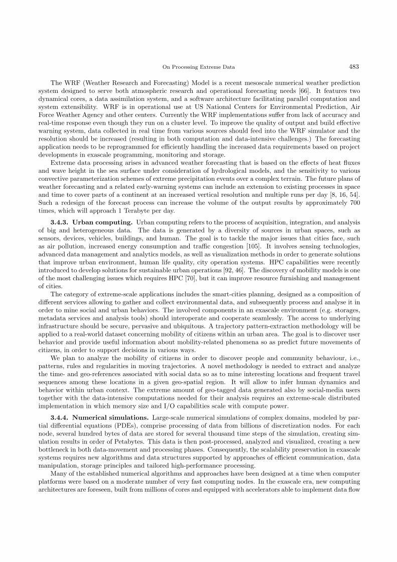
On Processing Extreme Data 483
The WRF (Weather Research and Forecasting) Model is a recent mesoscale numerical weather predictionsystem designed to serve both atmospheric research and operational forecasting needs [66]. It features twodynamical cores, a data assimilation system, and a software architecture facilitating parallel computation andsystem extensibility. WRF is in operational use at US National Centers for Environmental Prediction, AirForce Weather Agency and other centers. Currently the WRF implementations suffer from lack of accuracy andreal-time response even though they run on a cluster level. To improve the quality of output and build effectivewarning system, data collected in real time from various sources should feed into the WRF simulator and theresolution should be increased (resulting in both computation and data-intensive challenges.) The forecastingapplication needs to be reprogrammed for efficiently handling the increased data requirements based on projectdevelopments in exascale programming, monitoring and storage.
Extreme data processing arises in advanced weather forecasting that is based on the effects of heat fluxesand wave height in the sea surface under consideration of hydrological models, and the sensitivity to variousconvective parameterization schemes of extreme precipitation events over a complex terrain. The future plans ofweather forecasting and a related early-warning systems can include an extension to existing processes in spaceand time to cover parts of a continent at an increased vertical resolution and multiple runs per day [8, 16, 54].Such a redesign of the forecast process can increase the volume of the output results by approximately 700times, which will approach 1 Terabyte per day.
3.4.3. Urban computing. Urban computing refers to the process of acquisition, integration, and analysisof big and heterogeneous data. The data is generated by a diversity of sources in urban spaces, such assensors, devices, vehicles, buildings, and human. The goal is to tackle the major issues that cities face, suchas air pollution, increased energy consumption and traffic congestion [105]. It involves sensing technologies,advanced data management and analytics models, as well as visualization methods in order to generate solutionsthat improve urban environment, human life quality, city operation systems. HPC capabilities were recentlyintroduced to develop solutions for sustainable urban operations [92, 46]. The discovery of mobility models is oneof the most challenging issues which requires HPC [70], but it can improve resource furnishing and managementof cities.
The category of extreme-scale applications includes the smart-cities planning, designed as a composition ofdifferent services allowing to gather and collect environmental data, and subsequently process and analyse it inorder to mine social and urban behaviors. The involved components in an exascale environment (e.g. storages,metadata services and analysis tools) should interoperate and cooperate seamlessly. The access to underlyinginfrastructure should be secure, pervasive and ubiquitous. A trajectory pattern-extraction methodology will beapplied to a real-world dataset concerning mobility of citizens within an urban area. The goal is to discover userbehavior and provide useful information about mobility-related phenomena so as predict future movements ofcitizens, in order to support decisions in various ways.
We plan to analyze the mobility of citizens in order to discover people and community behaviour, i.e.,patterns, rules and regularities in moving trajectories. A novel methodology is needed to extract and analyzethe time- and geo-references associated with social data so as to mine interesting locations and frequent travelsequences among these locations in a given geo-spatial region. It will allow to infer human dynamics andbehavior within urban context. The extreme amount of geo-tagged data generated also by social-media userstogether with the data-intensive computations needed for their analysis requires an extreme-scale distributedimplementation in which memory size and I/O capabilities scale with compute power.
3.4.4. Numerical simulations. Large-scale numerical simulations of complex domains, modeled by par-tial differential equations (PDEs), comprise processing of data from billions of discretization nodes. For eachnode, several hundred bytes of data are stored for several thousand time steps of the simulation, creating sim-ulation results in order of Petabytes. This data is then post-processed, analyzed and visualized, creating a newbottleneck in both data-movement and processing phases. Consequently, the scalability preservation in exascalesystems requires new algorithms and data structures supported by approaches of efficient communication, datamanipulation, storage principles and tailored high-performance processing.
Many of the established numerical algorithms and approaches have been designed at a time when computerplatforms were based on a moderate number of very fast computing nodes. In the exascale era, new computingarchitectures are foreseen, built from millions of cores and equipped with accelerators able to implement data flow

484 D. Petcu, G. Iuhasz, D. Pop, D. Talia, J. Carretero, R. Prodan, T. Fahringer et al
approaches. The existing numerical methodologies and algorithms must follow these trends. For example, animplicit methodology is often preferred for the solution of PDEs because of longer possible time steps, however,because of the additional price for the solution of a large global linear system. An alternative approach, basedon explicit methods, requires only a matrix-vector multiplication in each time step. Even though the numberof time steps in explicit methods could be higher, such an approach could better fit the new architecture withmany smaller processing units resulting in a more efficient methodology.
One of the most complex fields of scientific computing is the computational fluid dynamics (CFD), whichis of great interest among researchers and engineers in many areas of science and technology. The core problemis the solution of the Navier-Stokes PDE equation or its variants, e.g., Darcy or Brinkman equation for flow inporous media. The CFD plays a crucial role in the modeling of many important industrial processes, e.g., heattransport-energy studies, solidification of advanced materials, microfluidics and nanofluidics, vehicles design,etc. The solution approaches that are based on local information from neighboring discretization nodes willbe preferred in exascale CFD solvers, because such methodologies are closer to natural behavior. Moreover,such approaches are tailored to the execution on exascale computer architectures that incorporate multi-levelprocessor and memory hierarchies, processing accelerators, and high-radix interconnection networks.
Solving extensive problems via local numerical methods requires efficient subdivision of the domain intoseveral million to several billion discretization nodes. Each simulation works on Terabytes of data, but evenmore data is stored for each simulation in form of checkpointing and simulation results. Each node produces itsown simulation data that can create substantial overhead if it has to be communicated to a centralized storage.Distributed storage in which nodes store data locally, or at least at a nearby storage location is preferable tocentralized storage at a single location that becomes an interconnection and storage bottleneck. Furthermore,distributed storage of results promotes distributed analysis and data visualization, which also proves highlyproblematic when working with Terabytes and Petabytes of data. Therefore, the data storage of the simulationprocedure should be planned with consideration of the optimal storage locations required.
3.5. Overview of the proposed methodology. Tables 3.1 and 3.2 summarize the proposed actionswhich were discussed in details in the previous subsections. In a concise way, they show the key actions to becarried out and the expected validations coming from some applications domains.
4. Conclusions. We provided in this paper a roadmap to reach the extreme-scale level in data processing.It is based on four pillars: new programming and energy models for extreme data applications, new toolsfor monitoring and data-analysis for extreme data applications, adaptation of data management and storagetechniques to extreme scale, and validation of the concepts and tools through specific extreme data applications.For each topic some limitations of the existing concepts and technologies have been identified and potentialsolutions to overcome these limitations were sketched without claiming that they guarantee the success or thatthey are the only solution. We recognize that the efforts to implement these solutions can be enormous and willrequire the joint efforts of multiple teams. Therefore we considered it useful to expose our ideas and proposalsin this paper and to seek for contributions in the proposed directions in the years to come.
REFERENCES
[1] J. Armstrong, Erlang, Communications of ACM, 53(9), September 2010.[2] A. Acosta, F. Almeida, Towards a Unified Heterogeneous Development Model in AndroidTM, Euro-Par 2013, 238-248[3] I. Ahmad, A. Abdulah, A. Alghamdi, Towards the Designing of a Robust Intrusion Detection System through an Optimized
Advancement of Neural Networks, Advances in Comp. Science and IT, Springer 2010.[4] M. Galea, M. Atkinson, C. S. Liew, P. Martin, Final Report on the ADMIRE Architecture. 2011[5] E. Alpaydin, Introduction to machine learning. The MIT Press, 2004.[6] J. Arnold, Software Defined Storage with OpenStack Swift, Amazon, 2013.[7] A. Barak, T. Ben-Nun, E. Levy A. Shiloh, A package for OpenCL based heterogeneous computing on clusters with many
GPU devices, 2010 IEEE Intl. Conf. on Cluster Computing Workshops and Posters, 17, 2010[8] A. Bartzokas, V. Kotroni, K. Lagouvardos, C.J. Lolis, A. Gkikas, M.I. Tsirogianni, Weather forecast in north-
western Greece: RISKMED warnings and verification of MM5 model, Natural Hazards and Earth System Sciences, 10,383-394, 2010.
[9] A. Bourdon, A. Noureddine, R. Rouvoy, L. Seinturier, Powerapi: A software library to monitor the energy consumedat the process level, ERCIM News 2013, no. 92.
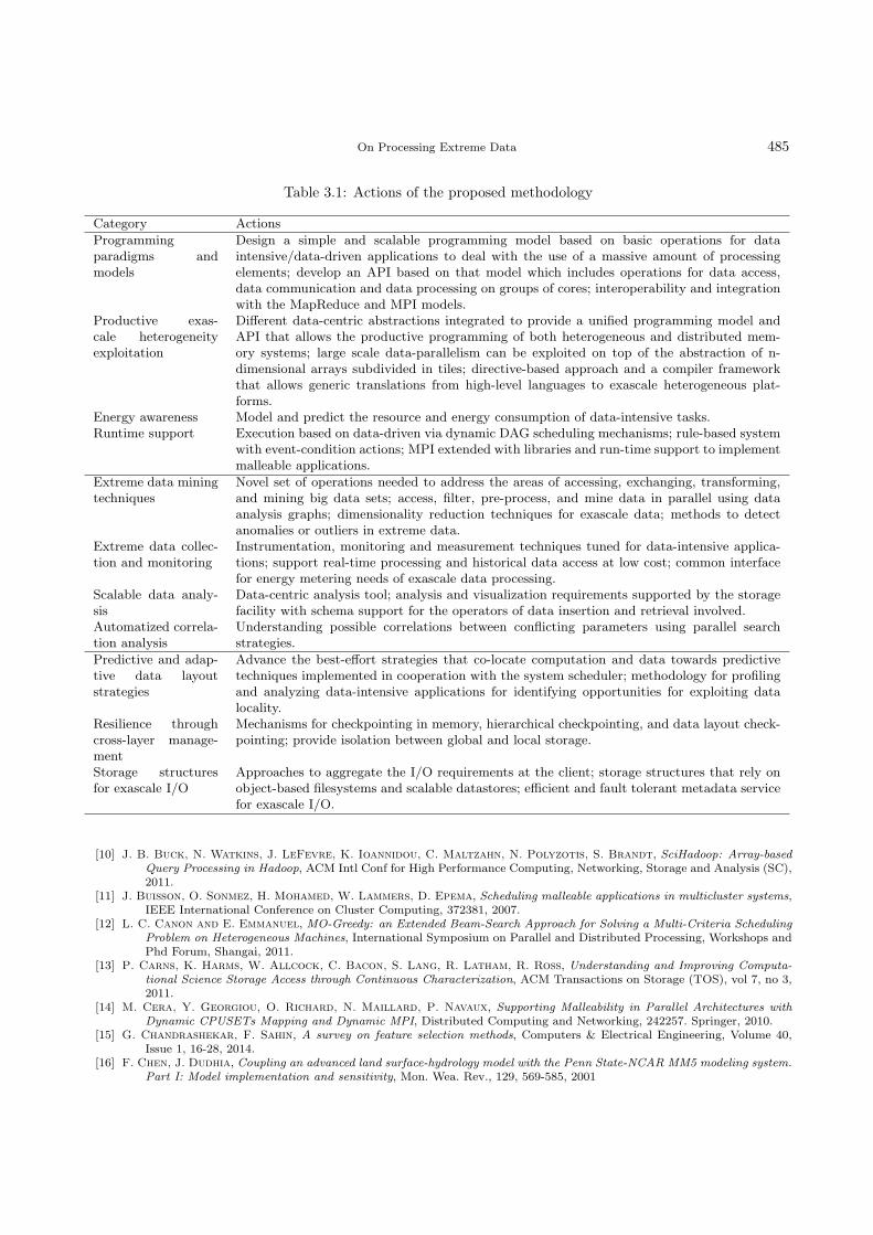
On Processing Extreme Data 485
Table 3.1: Actions of the proposed methodology
Category Actions
Programmingparadigms andmodels
Design a simple and scalable programming model based on basic operations for dataintensive/data-driven applications to deal with the use of a massive amount of processingelements; develop an API based on that model which includes operations for data access,data communication and data processing on groups of cores; interoperability and integrationwith the MapReduce and MPI models.
Productive exas-cale heterogeneityexploitation
Different data-centric abstractions integrated to provide a unified programming model andAPI that allows the productive programming of both heterogeneous and distributed mem-ory systems; large scale data-parallelism can be exploited on top of the abstraction of n-dimensional arrays subdivided in tiles; directive-based approach and a compiler frameworkthat allows generic translations from high-level languages to exascale heterogeneous plat-forms.
Energy awareness Model and predict the resource and energy consumption of data-intensive tasks.Runtime support Execution based on data-driven via dynamic DAG scheduling mechanisms; rule-based system
with event-condition actions; MPI extended with libraries and run-time support to implementmalleable applications.
Extreme data miningtechniques
Novel set of operations needed to address the areas of accessing, exchanging, transforming,and mining big data sets; access, filter, pre-process, and mine data in parallel using dataanalysis graphs; dimensionality reduction techniques for exascale data; methods to detectanomalies or outliers in extreme data.
Extreme data collec-tion and monitoring
Instrumentation, monitoring and measurement techniques tuned for data-intensive applica-tions; support real-time processing and historical data access at low cost; common interfacefor energy metering needs of exascale data processing.
Scalable data analy-sis
Data-centric analysis tool; analysis and visualization requirements supported by the storagefacility with schema support for the operators of data insertion and retrieval involved.
Automatized correla-tion analysis
Understanding possible correlations between conflicting parameters using parallel searchstrategies.
Predictive and adap-tive data layoutstrategies
Advance the best-effort strategies that co-locate computation and data towards predictivetechniques implemented in cooperation with the system scheduler; methodology for profilingand analyzing data-intensive applications for identifying opportunities for exploiting datalocality.
Resilience throughcross-layer manage-ment
Mechanisms for checkpointing in memory, hierarchical checkpointing, and data layout check-pointing; provide isolation between global and local storage.
Storage structuresfor exascale I/O
Approaches to aggregate the I/O requirements at the client; storage structures that rely onobject-based filesystems and scalable datastores; efficient and fault tolerant metadata servicefor exascale I/O.
[10] J. B. Buck, N. Watkins, J. LeFevre, K. Ioannidou, C. Maltzahn, N. Polyzotis, S. Brandt, SciHadoop: Array-basedQuery Processing in Hadoop, ACM Intl Conf for High Performance Computing, Networking, Storage and Analysis (SC),2011.
[11] J. Buisson, O. Sonmez, H. Mohamed, W. Lammers, D. Epema, Scheduling malleable applications in multicluster systems,IEEE International Conference on Cluster Computing, 372381, 2007.
[12] L. C. Canon and E. Emmanuel, MO-Greedy: an Extended Beam-Search Approach for Solving a Multi-Criteria SchedulingProblem on Heterogeneous Machines, International Symposium on Parallel and Distributed Processing, Workshops andPhd Forum, Shangai, 2011.
[13] P. Carns, K. Harms, W. Allcock, C. Bacon, S. Lang, R. Latham, R. Ross, Understanding and Improving Computa-tional Science Storage Access through Continuous Characterization, ACM Transactions on Storage (TOS), vol 7, no 3,2011.
[14] M. Cera, Y. Georgiou, O. Richard, N. Maillard, P. Navaux, Supporting Malleability in Parallel Architectures withDynamic CPUSETs Mapping and Dynamic MPI, Distributed Computing and Networking, 242257. Springer, 2010.
[15] G. Chandrashekar, F. Sahin, A survey on feature selection methods, Computers & Electrical Engineering, Volume 40,Issue 1, 16-28, 2014.
[16] F. Chen, J. Dudhia, Coupling an advanced land surface-hydrology model with the Penn State-NCAR MM5 modeling system.Part I: Model implementation and sensitivity, Mon. Wea. Rev., 129, 569-585, 2001

486 D. Petcu, G. Iuhasz, D. Pop, D. Talia, J. Carretero, R. Prodan, T. Fahringer et al
Table 3.2: Expected validations of the proposed actions by the selected applications
Category Earth obser-vation
Weather fore-cast
Urban com-puting
Numericalsimulations
Programming paradigms and models
Productive exascale heterogeneity exploitation
Energy awareness
Runtime support
Extreme data mining techniques
Extreme data collection and monitoring
Scalable data analysis
Automatized correlation analysis
Predictive and adaptive data layout strategies
Resilience through cross-layer management
Storage structures for exascale I/O
[17] Z. Chen, Y.F. Li, Anomaly Detection Based on Enhanced DBScan Algorithm, Procedia Engineering, 2011.[18] S. Conway, C. Dekate, E. Joseph, IDC HPC End-User Special Study of High-Performance Data Analysis (HPDA): Where
Big Data Meets HPC, Worldwide Study of HPC End-User Sites, 2013, www.idc.com[19] L. F. Cupertino, G. Da Costa, J.-M. Pierson, Towards a generic power estimator, Computer Science - Research and
Development, Springer Berlin / Heidelberg, Special Issue Ena-HPC 2014[20] P. Martin, G. Yaikhom, DISPEL: Users’ Manual, 2011, http://www.admire-project.eu/docs/DISPEL-manual.pdf[21] R. F. Vicente, I. Klampanos, A. Krause, M. David, A. Moreno, M. Atkinson, dispel4py: A Python Framework for Data-
Intensive Scientific Computing,2014 Data Intensive Scalable Computing Systems (DISCS-2014) workshop (SC14).2014[22] J. Dean and S. Ghemawat, Mapreduce: simplified data processing on large clusters, Commun. ACM, 51(1):107113, 2008.[23] Department of Energy, Cross-cutting Technologies for Computing at the Exascale, Washington, DC, Scientific Grand
Challenges Workshop Series, pp. 99, 2009. http://extremecomputing.labworks.org/crosscut/CrosscutWSFinalReptDraft02.pdf.
[24] Department of Energy, DOE Exascale Roadmap Highlights Big Data, 2014, http://www.hpcwire.com/2014/04/07/doe-exascale-roadmap-highlights-big-data/
[25] J. Dongarra, P. Beckman, T. Moore, P. Aerts et al, The International Exascale Software Project roadmap, Interna-tional J. of High Performance Computing Applications, 2011.
[26] D. Engel, L. Huttenberger, B. Hamann, A Survey of Dimension Reduction Methods for High-Dimensional Data Analysisand Visualization, Visualization of Large and Unstructured Data Sets: Applications in Geospatial Planning, Modelingand Engineering - Proceedings of IRTG Workshop, 2011
[27] M. Eshel, R. Haskin, D. Hildebrand, M. Naik, F. Schmuck, R. Tewari, Panache: A Parallel File System Cache forGlobal File Access, FAST 2010. Usenix,. 2010.
[28] European Technology Platform for High Performance Computing, ETP4HPC Strategic Research Agenda AchievingHPC leadership in Europe, Barcelona May 2013, www.etp4hpc.eu.
[29] European Technological Platform for High Performance Computing, Vision Paper, 2012[30] M.J. Flynn, O. Mencer, V. Milutinovic, G. Rakocevic, P. Stenstrom, R. Trobec, M. Valero, Moving from petaflops
to petadata, Communications of the ACM. 2013;56:39-42;[31] M.M. Gaber, A. Zaslavsky, S. Krishnaswamy, Mining data streams: a review, ACM Sigmod Record, volume 34, number
2, 18-26, ACM, 2005.[32] T. Gamblin, B.R. De Supinski, M. Schulz, R. Fowler, D.A. Reed, Clustering performance data efficiently at massive
scales, 24th ACM International Conference on Supercomputing, 243-252, ACM, 2010.[33] C. George, S. S. Vadhiyar, ADFT: An adaptive framework for fault tolerance on large scale systems using application
malleability, Procedia Computer Science 9 (0) (2012) 166 175, Proceedings of the International Conference on Compu-tational Science, ICCSg 2012. doi: 10.1016/j.procs.2012.04.018.
[34] S. Ghemawat, H. Gobioff, and S.-T. Leung, The google file system, Proceedings of the nineteenth ACM symposium onOperating systems principles, SOSP 03, 2943, ACM, 2003.
[35] I. Grasso, S. Pellegrini, B. Cosenza, T. Fahringer, LibWater: heterogeneous distributed computing made easy, ICS2013: 161-172, 2013
[36] W. Gropp, M. Snir, Programming for Exascale Computers, Computing in Science & Engineering, vol.15, no. 6, 27-35, 2013.[37] HDF group, HDF5, http://www.hdfgroup.org/hdf5/.[38] J. He, J. Bent, A. Torres, G. Grider, G. Gibson, C. Maltzahn, X.-H. Sun, I/O Acceleration with Pattern Detection,
ACM Symp on High-Performance Parallel and Distributed Computing (HPDC), 2013.[39] High Performance and Embedded Architecture and Compilation Consortium, HiPEAC Roadmap, 2011,
www.hipeac.net/roadmap[40] C.-L. Huang, J.-F. Dun, A distributed PSOSVM hybrid system with feature selection and parameter optimization, Applied

On Processing Extreme Data 487
Soft Computing, Vol. 8, Issue 4, 1381-1391, 2008[41] J. Hungershofer, On the combined scheduling of malleable and rigid jobs, Proceedings of the 16th Symposium on Computer
Architecture and High Performance Computing (SBAC-PAD 2004), 206213, 2004.[42] IBM, GPFS. General Parallel File System, Efficient storage management for big data applications, http://www.ibm.com/
systems/software/gpfs.[43] H. H. Inbarani, A. T. Azar, G. Jothi, Supervised hybrid feature selection based on PSO and rough sets for medical
diagnosis, Computer Methods and Programs in Biomedicine, Vol. 113, Issue 1, 175-185, 2014.[44] F. Isaila, J. Garcia, J. Carretero, R.B. Ross, D. Kimpe, Making the Case for Reforming the I/O Software Stack of
Extreme-Scale Systems,Technical Report. Argonne Labs, IL, USA, 2014.[45] F. Jemili, M. Zaghdoud, M. Ben Ahmed, A Framework for an Adaptive Intrusion Detection System using Bayesian
Network, Intelligence and Security Informatics, 2007.[46] A. Jimenez-Molina and I.-Y. Ko, Spontaneous task composition in urban computing environments based on social, spatial,
and temporal aspects, Eng. Appl. Artif. Intell. 24, 8 2011, 1446-1460.[47] Md. M. Kabir, Md. M. Islam, K. Murase, A new wrapper feature selection approach using neural network, Neurocom-
puting, Vol. 73, Issues 1618, 3273-3283, 2010.[48] Y. Kessaci, N. Melab and E.-G. Talbi, A multi-start local search heuristic for an energy efficient VMs assignment on
top of the OpenNebula Cloud manager, Future Generation Computer Systems 36, 237-256, 2014.[49] A. K. M. Khaled, A. Talukder, M. Kirley and R. Buyya, Multiobjective differential evolution for scheduling workflow
applications on global Grids, Concurrency and Computation: Practice & Experience, vol. 21, no. 13, 1742-1756, 2009.[50] L. Khan, M. Awad, B. Thuraisingham, A New Intrusion Detection System Using Support Vector Machines and Hierar-
chical Clustering,The VLDB Journal, 2007.[51] V. R. Khare, X. Yao and K. Deb, Performance Scaling of Multi-Objective Evolutionary Algorithms,Conference on Evolu-
tionary Multi-Criterion Optimization, 2003.[52] Kufrin, R. Perfsuite, An accessible, open source performance analysis environment for Linux, 6th International Confer-
ence on Linux Clusters: The HPC Revolution, volume 151, p 5, 2005.[53] M. Kumar, M. Hanumanthappa, T. Kumar, Intrusion Detection System using decision tree algorithm, IEEE 14th Inter-
national Conference on Communication Technology (ICCT), 2012.[54] G. Korres, A. Papadopoulos, P. Katsafados, D. Ballas, L. Perivoliotis, K. Nittis, A 2-year intercomparison of
the WAM-Cycle4 and the WAVEWATCH-III wave models implemented within the Mediterranean Sea, MediterraneanMarine Science 12(1), 129-152, 2011
[55] J. Li, W.-k. Liao, A. Choudhary, R. Ross, R. Thakur, W. Gropp, R. Latham, A. Siegel, B. Gallagher, M. Zin-
gale, Parallel netcdf: A high-performance scientific i/o interface, Proceedings of the 2003 ACM/IEEE conference onSupercomputing, p. 39, ACM, 2003.
[56] P. Llopis, F.J. Garca-Blas, F. Isaila, J. Carretero, VIDAS: Object-based Virtualized Data Sharing for High Perfor-mance Storage I/O, Proceedings of the ACM ScienceCloud’13, 2013.
[57] G. Llort, J. Gonzalez, H. Servat, J. Gimenez, J. Labarta, On-line detection of large-scale parallel application’s structure,2010 IEEE International Symposium on Parallel & Distributed Processing (IPDPS), p 1-10, 2010
[58] T.V. Luong, N. Melab, E.-G. Talbi, GPU-Based multi-start local search algorithms, Learning and Intelligent Optimization.6683, 321-335. 2011, Springer.
[59] T.V. Luong, N. Melab, E.-G. Talbi, GPU computing for parallel local search metaheuristic algorithms, Transactions onComputers 62, 173-185, 2013
[60] Lustre, High Performance and Scalability, http://www.lustre.org.[61] K. El Maghraoui, T.J. Desell, B.K. Szymanski, C. A. Varela, Malleable iterative MPI applications, Concurrency
Computat.: Pract. Exper., 21(3): 393413, 2009.[62] J. Mair, Z. Huang, D. Eyers, L. F. Cupertino, G. Da Costa, J.-M. Pierson, H. Hlavacs, Power Modeling, Large-Scale
Distributed Systems and Energy Efficiency: A holistic view. Jean-Marc Pierson (Eds.), John Wiley and Sons, 5, March2015
[63] S. Matsuoka, H. Sato, O. Tatebe, M. Koibuchi, I. Fujiwara, S.Suzuki, et al, Extreme Big Data (EBD): Next Gener-ation Big Data Infrastructure Technologies Towards Yottabyte, Supercomputing Frontiesr and Innovations, vol. 1, no.2, 2014, 89-107
[64] N. Melab, K. Boufaras, E.-G. Talbi, et al, ParadisEO-MO-GPU: a framework for parallel GPU-based local searchmetaheuristics, Proceeding of the 15th annual conference on Genetic and evolutionary computation conference, 1189-1196. ACM, 2013.
[65] D. Mey, S. Biersdorf, C. Bischof, K. Diethelm, D. Eschweiler, M. Gerndt, A. Knpfer, D. Lorenz, A. Malony,
W.E. Nagel, et al, Score-P: A Unified Performance Measurement System for Petascale Applications, Competence inHigh Performance Computing 2010, 85-97, Springer, 2012.
[66] J. Michalakes, J. Dudhia, D. Gill, T. Henderson, J. Klemp, W. Skamarock, W. Wang, The Weather Research andForecast Model: Software Architecture and Performance, 11th ECMWF Workshop on the Use of High PerformanceComputing In Meteorology, 2004.
[67] B.P. Miller, M.D. Callaghan, J.M. Cargille, J.K. Hollingsworth, R.B. Irvin, K.L. Karavanic, K.L., K. Kun-
chithapadam, T. Newhall, The Paradyn parallel performance measurement tool, Computer, vol. 28, no. 11, 37-46,1995.
[68] Mpi forum, High-end-computing systems, http://www.mpi-forum.org/.[69] C. Modi, D. Patel, B. Borisaniya, H. Patel, A. Patel, M. Rajarajan, A survey of intrusion detection techniques in
Cloud, Journal of Network and Computer Applications, 2013.

488 D. Petcu, G. Iuhasz, D. Pop, D. Talia, J. Carretero, R. Prodan, T. Fahringer et al
[70] M. Nanni, R. Trasarti, G. Rossetti, D. Pedreschi, Efficient distributed computation of human mobility aggregatesthrough user mobility profiles, Proceedings of the ACM SIGKDD International Workshop on Urban Computing (Urb-Comp ’12), 2012, 87-94.
[71] J. Nieplocha, B. Palmer, V. Tipparaju, M. Krishnan, H. Trease, E. Apra, Advances, Applications and Performanceof the Global Arrays Shared Memory Programming Toolkit, Intl. J. of High Performance Computing Applications 20(2):203-23, 2006.
[72] R.V. van Nieuwpoort, J.W. Romein, Correlating Radio Astronomy Signals with Many-Core Hardware, Intl. J. of ParallelProgramming 39(1), 88114, 2011.
[73] R.W. Numrich, J. Reid, Co-array Fortran for parallel programming, ACM SIGPLAN FORTRAN Forum 17(2):131, 1998.[74] PlanetHPC, Strategy for Research and Innovation through HPC, November 2011, http://www.planethpc.eu/images/
stories/planethpc-strategy2.pdf[75] Partnership for Advanced Computing in Europe, PRACE Scientific Case 2012-2020, October 2012, www.prace-
ri.eu/PRACE-The-Scientific-Case-for-HPC[76] J. E. Pecero, P. Bouvry, H. J. Fraire Huacuja, S.U. Khan, A Multi-objective GRASP Algorithm for Joint Opti-
mization of Energy Consumption and Schedule Length of Precedence-Constrained Applications, 9th IEEE InternationalConference on Dependable, Autonomic and Secure Computing, 2011.
[77] Orange, Orangefs/pvfs, http://www.pvfs.org.[78] R Core Team, R: A Language and Environment for Statistical Computing, R Foundation for Statistical Computing, Vienna,
Austria, 2014[79] I.Raicu, I.T. Foster, P. Beckman, Making a case for distributed file systems at exascale, 3rd International workshop on
Large-scale system and application performance, LSAP 11, 1118, ACM, 2011.[80] P.C. Roth, B.P. Miller, On-line automated performance diagnosis on thousands of processes, 11th ACM SIGPLAN
symposium on Principles and practice of parallel programming, 69-80, ACM, 2006.[81] R. Reyes, I. Lpez-Rodrguez, J.J. Fumero, F. de Sande, accULL: An OpenACC Implementation with CUDA and OpenCL
Support, Euro-Par 2012, 871-882, 2012.[82] S.S. Shende, A.D. Malony, The Tau Parallel Performance System, International Journal of High Performance Computing
Applications, vol. 20, no. 2, 287-311, 2006.[83] D. Singh and R. Garg, A robust multi-objective optimization to workflow scheduling for dynamic grid, International
Conference on Advances in Computing and Artificial Intelligence, 183-188, 2011.[84] M. Snir, R.W. Wisniewski, J.A. Abraham, S.V. Adve, S. Bagchi et al, Addressing Failures in Exascale Computing,
Tech. Report ANL/MCS-TM-332, Argonne Nat’l Laboratory, Mathematics and Computer Science Division, Apr. 2013.[85] R. Hill, SPRINT: A new parallel framework for R, BMC Bioinformatics. 2008[86] R. Sudarsan, C. J. Ribbens, ReSHAPE: A Framework for Dynamic Resizing and Scheduling of Homogeneous Applications
in a Parallel Environment, International Conference on Parallel Processing, ICPP 2007, 44-44, 2007.[87] C. Sweetlin Hemalatha, V. Vaidehi, R. Lakshmi, Minimal infrequent pattern based approach for mining outliers in data
streams, Expert Systems with Applications, on-line October 2014[88] I. Syarif, A. Prugel-Bennett, G. Wills, Unsupervised Clustering Approach for Network Anomaly Detection, Networked
Digital Technologies, Springer 2012.[89] A. K. A. Talukder, M. Kirley, R. Buyya, Multiobjective Differential Evolution for Workflow Execution on Grids, 5th
International Workshop on Middleware for Grid Computing, California, 2007.[90] C. J. Tan, C.P. Lim, Y.N Cheah, A multi-objective evolutionary algorithm-based ensemble optimizer for feature selection
and classification with neural network models, Neurocomputing, Vol. 125, 217-228, 2014.[91] W. Tantisiriroj, S. Patil, G. Gibson, S. W. Son, S. J. Lang, R. B. Ross, On the Duality of Data-intensive File System
Design: Reconsiling HDFS and PVFS, ACM Intl Conf for High Performance Computing, Networking, Storage andAnalysis (SC), 2011.
[92] A. Tenschert, M. Assel, A. Cheptsov, G. Gallizo, E.D. Valle, I. Celino, Parallelization and Distribution Techniquesfor Ontology Matching in Urban Computing Environments, Proceedings of OM 2009.
[93] C. Tsotskas, T. Kipouros, A.M. Savill, The Design and Implementation of a GPU-enabled Multi-objective Tabu-searchIntended for Real World and High-dimensional Applications, Procedia Computer Science, Vol. 29, 2152-2161, 2014.
[94] D. Talia, P. Trunfio, O. Verta, The Weka4WS Framework for Distributed Data Mining in Service-oriented Grids,Concurrency and Computation: Practice and Experience. 20(16): 1933-1951, 2008
[95] UPC Consortium, UPC language specifications v1.2, 2005.[96] VERCE consortium, VERCE, http://www.verce.eu/[97] M.Vinas, Z. Bozkus, B.B. Fraguela, Exploiting heterogeneous parallelism with the Heterogeneous Programming Library,
J. Parallel Distrib. Comput. 73(12): 1627-1638, 2013.[98] M. Wachs, M. Abd-El-Malek, E. Thereska, G. R. Ganger, Argon: performance insulation for shared storage servers,
USENIX Conf. on File and Storage Technologies (FAST), 61-76, 2007.[99] M. Hall, E. Frank, G. Holmes, B. Pfahringer, P. Reutemann, I. H. Witten, The WEKA Data Mining Software: An
Update, SIGKDD Explorations, Volume 11, Issue 1. 2009[100] X. Wang, R. Buyya and J. Su, Reliability-Oriented Genetic Algorithm for Workflow Applications using Max-Min Strategy,
9th International Symposium on Cluster Computing and the Grid, 2009.[101] H. Xia, J. Zhuang, D. Yu, Multi-objective unsupervised feature selection algorithm utilizing redundancy measure and
negative epsilon-dominance for fault diagnosis, Neurocomputing, Vol. 146, 113-124, 2014.[102] H. Yoon, C.-S. Park, J. S. Kim, J.-G. Baek, Algorithm learning based neural network integrating feature selection and
classification, Expert Systems with Applications, Vol. 40, Issue 1, 231-241, 2013.

On Processing Extreme Data 489
[103] H. Yu, R. Chen, G. Zhang, A SVM Stock Selection Model within PCA, Procedia Computer Science, Vol. 31, 406-412, 2014.[104] J. Yu, M. Kirley and R. Buyya, Multi-Objective Planning for Workflow Execution on Grids, 8th International Conference
on Grid Computing, 2007.[105] Yu Zheng, Licia Capra, Ouri Wolfson, Hai Yang, Urban Computing: concepts, methodologies, and applications, ACM
Transaction on Intelligent Systems and Technology (ACM TIST). 2014[106] T. Zhu, A. Tumanov, M. A. Kozuch, M. Harchol-Balter, G. R. Ganger, PriorityMeister: Tail Latency QoS for Shared
Neworked Storage, ACM Symp. Cloud Computing (SoCC), 2014.
Edited by: Viorel NegruReceived: December 16, 2015Accepted: January 16, 2016


AIMS AND SCOPE
The area of scalable computing has matured and reached a point where new issues and trends require a pro-fessional forum. SCPE will provide this avenue by publishing original refereed papers that address the presentas well as the future of parallel and distributed computing. The journal will focus on algorithm development,implementation and execution on real-world parallel architectures, and application of parallel and distributedcomputing to the solution of real-life problems. Of particular interest are:
Expressiveness:
• high level languages,• object oriented techniques,• compiler technology for parallel computing,• implementation techniques and their effi-ciency.
System engineering:
• programming environments,• debugging tools,• software libraries.
Performance:
• performance measurement: metrics, evalua-tion, visualization,
• performance improvement: resource allocationand scheduling, I/O, network throughput.
Applications:
• database,
• control systems,
• embedded systems,
• fault tolerance,
• industrial and business,
• real-time,
• scientific computing,
• visualization.
Future:
• limitations of current approaches,
• engineering trends and their consequences,
• novel parallel architectures.
Taking into account the extremely rapid pace of changes in the field SCPE is committed to fast turnaroundof papers and a short publication time of accepted papers.
INSTRUCTIONS FOR CONTRIBUTORS
Proposals of Special Issues should be submitted to the editor-in-chief.The language of the journal is English. SCPE publishes three categories of papers: overview papers,
research papers and short communications. Electronic submissions are preferred. Overview papers and shortcommunications should be submitted to the editor-in-chief. Research papers should be submitted to the editorwhose research interests match the subject of the paper most closely. The list of editors’ research interests canbe found at the journal WWW site (http://www.scpe.org). Each paper appropriate to the journal will berefereed by a minimum of two referees.
There is no a priori limit on the length of overview papers. Research papers should be limited to approx-imately 20 pages, while short communications should not exceed 5 pages. A 50–100 word abstract should beincluded.
Upon acceptance the authors will be asked to transfer copyright of the article to the publisher. Theauthors will be required to prepare the text in LATEX2ε using the journal document class file (based on theSIAM’s siamltex.clo document class, available at the journal WWW site). Figures must be prepared inencapsulated PostScript and appropriately incorporated into the text. The bibliography should be formattedusing the SIAM convention. Detailed instructions for the Authors are available on the SCPE WWW site athttp://www.scpe.org.
Contributions are accepted for review on the understanding that the same work has not been publishedand that it is not being considered for publication elsewhere. Technical reports can be submitted. Substantiallyrevised versions of papers published in not easily accessible conference proceedings can also be submitted. Theeditor-in-chief should be notified at the time of submission and the author is responsible for obtaining thenecessary copyright releases for all copyrighted material.


![Scalable Computing - SCPE · 1. Introduction. Geometric Topology deals with piecewise-linear (PL) n-manifolds [2], i.e. compact topological manifolds for which there is a triangulation](https://img.pdfslide.us/doc/110x75/5f1fa4a3d0989c77af1bc9bf/scalable-computing-scpe-1-introduction-geometric-topology-deals-with-piecewise-linear.jpg)