Scalable Auto-Encoders for Gravitational Waves

Detection from Time Series Data

Roberto Corizzo, Michelangelo Ceci, Eftim Zdravevski, Nathalie Japkowicz

Introduction

Challenges in GW detection

To effectively carry out manual filtering operations, we need to know the underlying type of noise, as well as which frequencies could be relevant (or irrelevant) for the detection of a GW.

Additional knowledge is required to perform other recurrent tasks, such as spectrogram analysis, filtering, and whitening.

Large volumes of data, in terms of petabytes per day, are collected by detectors

We investigated:

Two approaches (one supervised, one unsupervised) working directly on strain data

Auto-encoder models to classify strain time series data with an anomaly detection strategy

Auto-encoders for feature extraction and then a classification with Gradient-Boosted Trees (GBTs)

The goal was discard noise time series and identify time series that could contain a real phenomenon – a classification problem

Our approaches do not require any pre-processing step (e.g., generation of spectrograms, filtering and whitening) and use real annotated GW events

The proposed approaches utilized Apache Spark framework for scalable computation

2

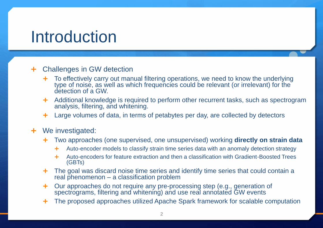
The problem

Whitened time series representation of the

same GWs signal (ID GW151226).

3

The strain time series representing real GWs

immersed in noise are impossible to

distinguish, even for the human eye, if no data

pre-processing is carried out.

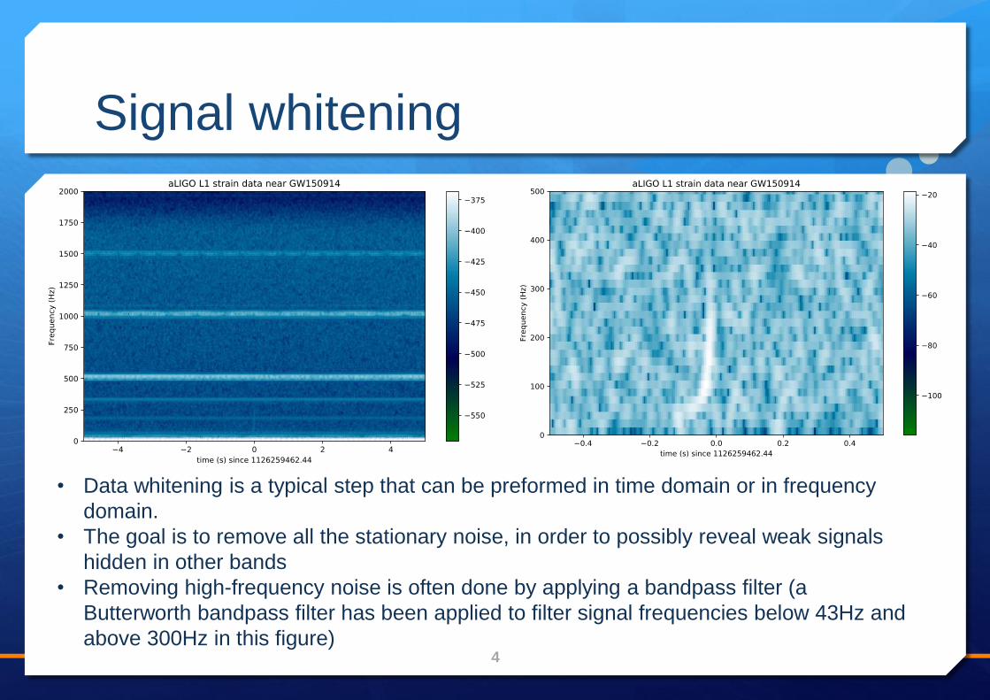
Signal whitening

4

• Data whitening is a typical step that can be preformed in time domain or in frequency

domain.

• The goal is to remove all the stationary noise, in order to possibly reveal weak signals

hidden in other bands

• Removing high-frequency noise is often done by applying a bandpass filter (a

Butterworth bandpass filter has been applied to filter signal frequencies below 43Hz and

above 300Hz in this figure)

Binary classification as anomaly

detection with autoencoders

When the data belongs to two classes, the binary classification task can be reformulated as an unsupervised anomaly detection task, detecting whether it’s normal or anomaly

The purpose is to discriminate among two classes by analyzing data over time and classify if the current behavior is as expected (normal) or it deviates from the expected distribution (anomaly).

The task can be reformulated as an unsupervised anomaly detection task

Auto-encoders have demonstrated superior performance in recent literature

They are able to build representations with a low reconstruction error, based on non-linear combinations of input features

5

Methods

6

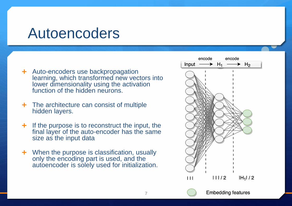
Autoencoders

Auto-encoders use backpropagation learning, which transformed new vectors into lower dimensionality using the activation function of the hidden neurons.

The architecture can consist of multiple hidden layers.

If the purpose is to reconstruct the input, the final layer of the auto-encoder has the same size as the input data

When the purpose is classification, usually only the encoding part is used, and the autoencoder is solely used for initialization.

7

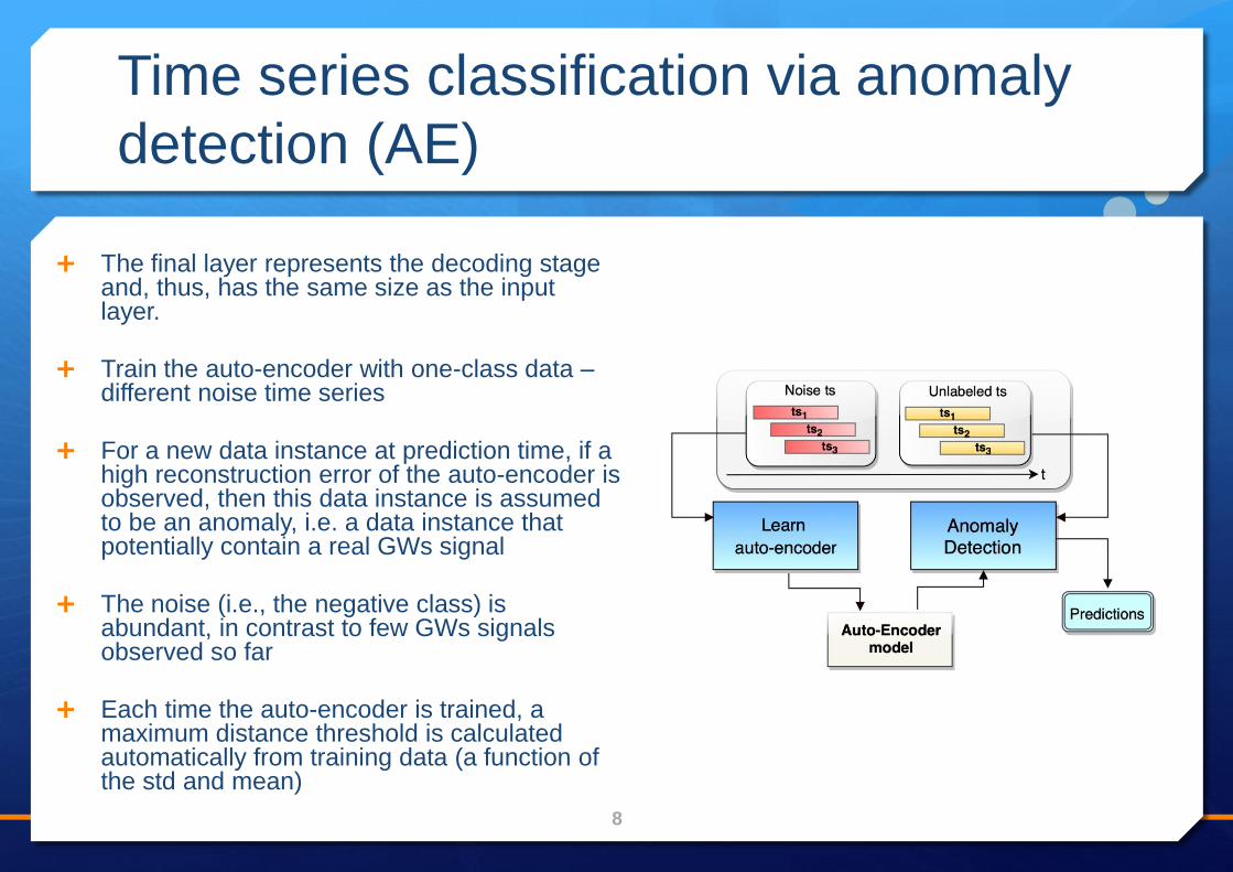
Time series classification via anomaly

detection (AE)

The final layer represents the decoding stage and, thus, has the same size as the input layer.

Train the auto-encoder with one-class data –different noise time series

For a new data instance at prediction time, if a high reconstruction error of the auto-encoder is observed, then this data instance is assumed to be an anomaly, i.e. a data instance that potentially contain a real GWs signal

The noise (i.e., the negative class) is abundant, in contrast to few GWs signals observed so far

Each time the auto-encoder is trained, a maximum distance threshold is calculated automatically from training data (a function of the std and mean)

8

Feature extraction with supervised

classification (AE-GBT)

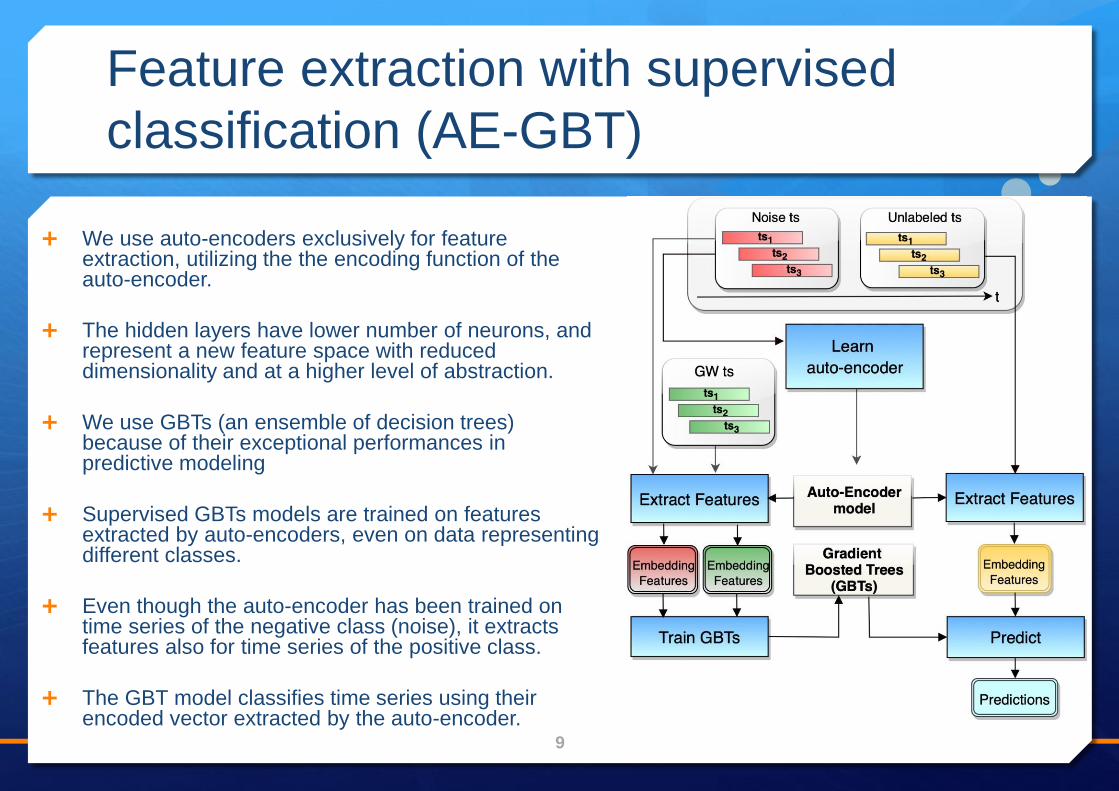
We use auto-encoders exclusively for feature extraction, utilizing the the encoding function of the auto-encoder.

The hidden layers have lower number of neurons, and represent a new feature space with reduced dimensionality and at a higher level of abstraction.

We use GBTs (an ensemble of decision trees) because of their exceptional performances in predictive modeling

Supervised GBTs models are trained on features extracted by auto-encoders, even on data representing different classes.

Even though the auto-encoder has been trained on time series of the negative class (noise), it extracts features also for time series of the positive class.

The GBT model classifies time series using their encoded vector extracted by the auto-encoder.

9

Experimental setup

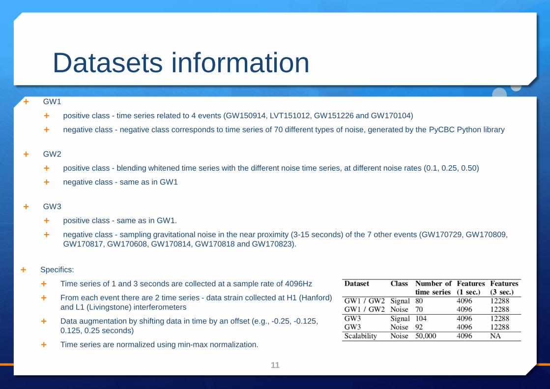
Datasets information GW1

positive class - time series related to 4 events (GW150914, LVT151012, GW151226 and GW170104)

negative class - negative class corresponds to time series of 70 different types of noise, generated by the PyCBC Python library

GW2

positive class - blending whitened time series with the different noise time series, at different noise rates (0.1, 0.25, 0.50)

negative class - same as in GW1

GW3

positive class - same as in GW1.

negative class - sampling gravitational noise in the near proximity (3-15 seconds) of the 7 other events (GW170729, GW170809,

GW170817, GW170608, GW170814, GW170818 and GW170823).

11

Specifics:

Time series of 1 and 3 seconds are collected at a sample rate of 4096Hz

From each event there are 2 time series - data strain collected at H1 (Hanford)

and L1 (Livingstone) interferometers

Data augmentation by shifting data in time by an offset (e.g., -0.25, -0.125,

0.125, 0.25 seconds)

Time series are normalized using min-max normalization.

Experimental setup

Auto-encoder (1 or 2 hidden layers for encoding and 1 or 2 hidden layers for decoding).

One hidden layer: hidden units is set to 512 or 1024

Two hidden layers, the hidden units is set to:

512 for the first layer, and 256 for the second layer,

1024 for the first layer, and 512 for the second layer.

Considering the sampling rate of 4096Hz, 512 hidden units correspond to 1/8 of the 1-second time series length, or 1/24 of the 3 seconds time series length

GW1 and GW2 datasets - 5-fold CV

GW3 dataset - leave-one-event-out CV (4 events in the + class => 4-fold CV)

12

Other details:

The auto-encoder training uses the LBFGS optimizer

Maximum number of iterations = 500

Early stopping if the algorithm is unable to reduce the training error by 10e-5 at a certain iteration

In detection mode, the factor for the standard deviation to f=1.5 (empirically determined)

GBT parameters – default in MLlib : maxIter = 10, maxDepth = 5, maxBins = 32, minInstancesPerNode = 1, lossType = logistic.

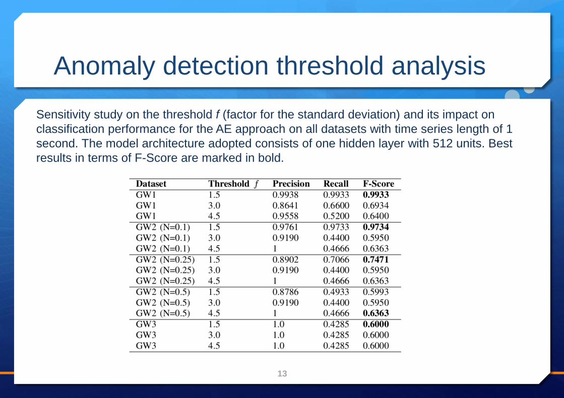
Anomaly detection threshold analysis

13

Sensitivity study on the threshold f (factor for the standard deviation) and its impact on

classification performance for the AE approach on all datasets with time series length of 1

second. The model architecture adopted consists of one hidden layer with 512 units. Best

results in terms of F-Score are marked in bold.

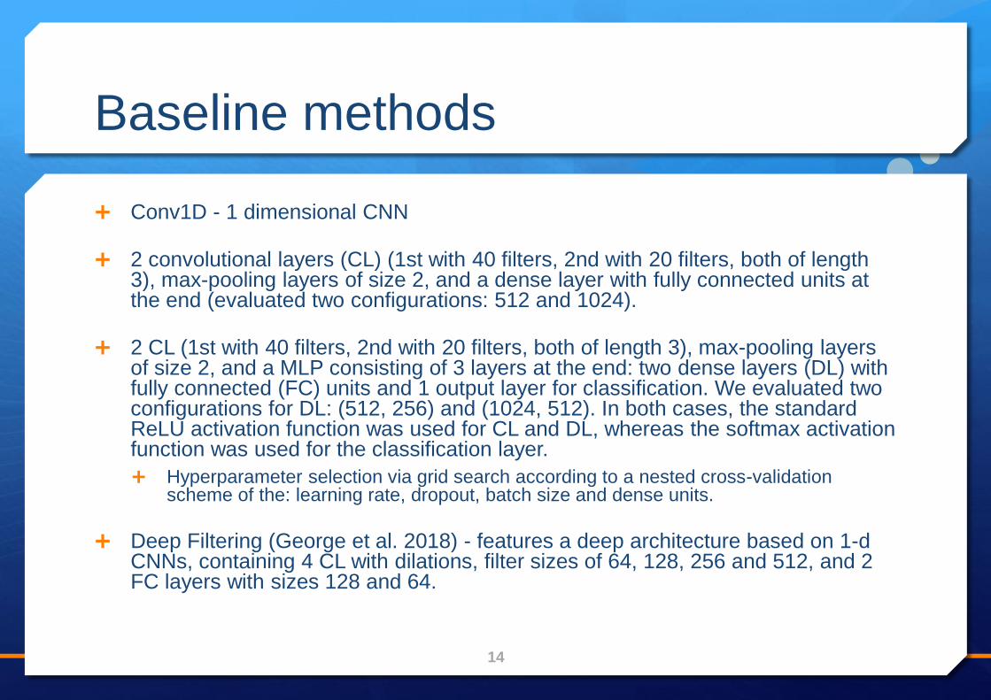
Baseline methods

Conv1D - 1 dimensional CNN

2 convolutional layers (CL) (1st with 40 filters, 2nd with 20 filters, both of length 3), max-pooling layers of size 2, and a dense layer with fully connected units at the end (evaluated two configurations: 512 and 1024).

2 CL (1st with 40 filters, 2nd with 20 filters, both of length 3), max-pooling layers of size 2, and a MLP consisting of 3 layers at the end: two dense layers (DL) with fully connected (FC) units and 1 output layer for classification. We evaluated two configurations for DL: (512, 256) and (1024, 512). In both cases, the standard ReLU activation function was used for CL and DL, whereas the softmax activation function was used for the classification layer.

Hyperparameter selection via grid search according to a nested cross-validation scheme of the: learning rate, dropout, batch size and dense units.

Deep Filtering (George et al. 2018) - features a deep architecture based on 1-d CNNs, containing 4 CL with dilations, filter sizes of 64, 128, 256 and 512, and 2 FC layers with sizes 128 and 64.

14

Results

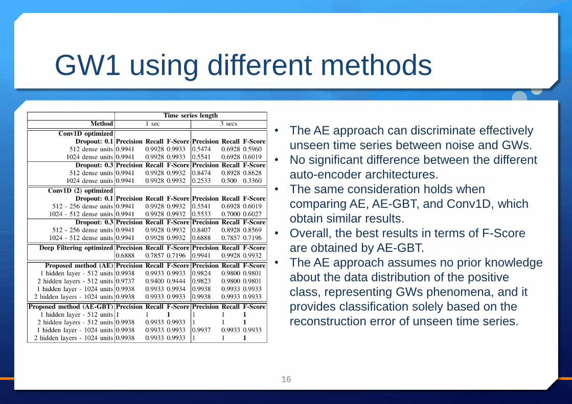
GW1 using different methods

16

• The AE approach can discriminate effectively

unseen time series between noise and GWs.

• No significant difference between the different

auto-encoder architectures.

• The same consideration holds when

comparing AE, AE-GBT, and Conv1D, which

obtain similar results.

• Overall, the best results in terms of F-Score

are obtained by AE-GBT.

• The AE approach assumes no prior knowledge

about the data distribution of the positive

class, representing GWs phenomena, and it

provides classification solely based on the

reconstruction error of unseen time series.

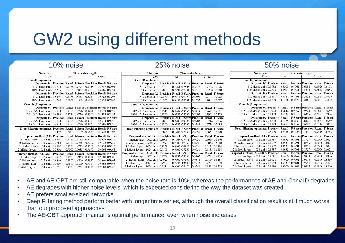
GW2 using different methods

17

10% noise 25% noise 50% noise

• AE and AE-GBT are still comparable when the noise rate is 10%, whereas the performances of AE and Conv1D degrades

• AE degrades with higher noise levels, which is expected considering the way the dataset was created.

• AE prefers smaller-sized networks.

• Deep Filtering method perform better with longer time series, although the overall classification result is still much worse

than our proposed approaches.

• The AE-GBT approach maintains optimal performance, even when noise increases.

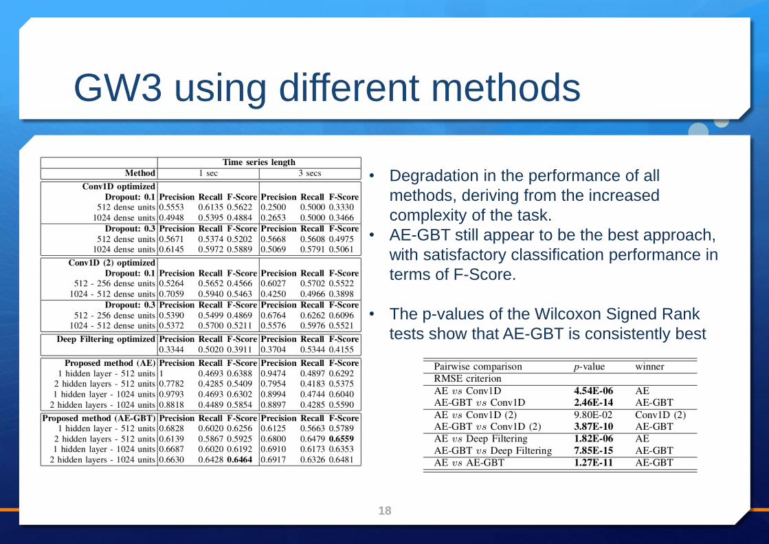
GW3 using different methods

18

• Degradation in the performance of all

methods, deriving from the increased

complexity of the task.

• AE-GBT still appear to be the best approach,

with satisfactory classification performance in

terms of F-Score.

• The p-values of the Wilcoxon Signed Rank

tests show that AE-GBT is consistently best

Scalability experimental setup

Scalability of GBT is well documented within Spark MLLib

Therefore, the focus is on the AE approach, which is utilized in both proposed approaches

We replicated all negative class time series of 1 sec. length from the GW1 dataset, resulting in up to 50.000 instances of time series that have at most 1% perturbation of each element of the time series. This was done to prevent unrealistically fast convergence of the loss function.

We used two Spark cluster configurations on Microsoft Azure HDInsight using D12, D13 and D14 instances (D12 has 4 cores, 28 GB of RAM, a D13 instance has 8 cores and 56 GB of RAM, and a D14 instance has 16 cores and 112 GB RAM.)

For the local setting, we use 2 D12 head nodes, and one D12 worker node.

1st cluster configuration: 2 D12 head nodes and 4 D13 worker nodes (scale factor=8)

2nd cluster configuration: 2 D12 head nodes and 8 D14 worker nodes (scale factor=16)

We evaluated different configurations for the Spark job, including the number of executors, the number of executor cores, and the executor memory.

19

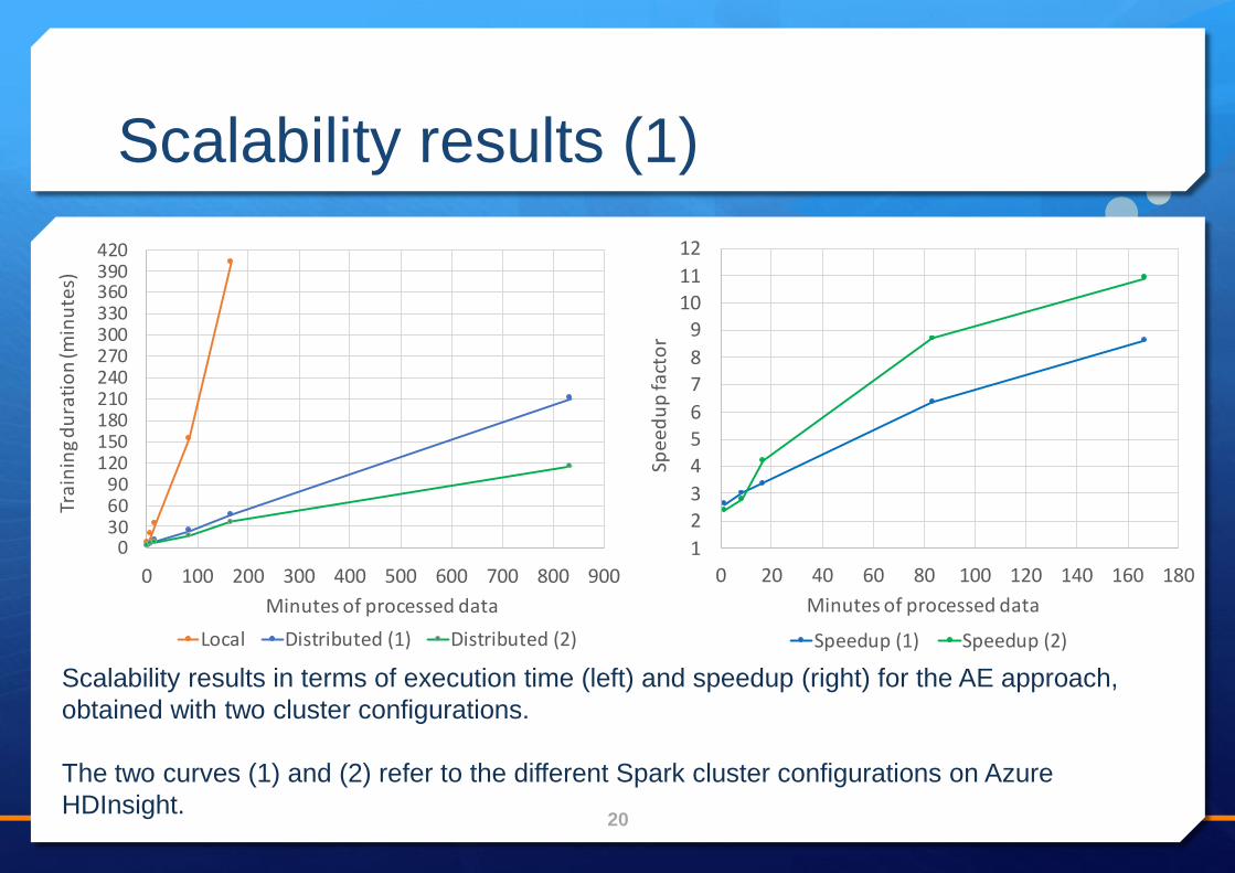
Scalability results (1)

20

0306090

120150180210240270300330360390420

0 100 200 300 400 500 600 700 800 900

Trai

nin

g d

ura

tio

n (m

inu

tes)

Minutes of processed data

Local Distributed (1) Distributed (2)

1

2

3

4

5

6

7

8

9

10

11

12

0 20 40 60 80 100 120 140 160 180

Spe

ed

up

fact

or

Minutes of processed data

Speedup (1) Speedup (2)

Scalability results in terms of execution time (left) and speedup (right) for the AE approach,

obtained with two cluster configurations.

The two curves (1) and (2) refer to the different Spark cluster configurations on Azure

HDInsight.

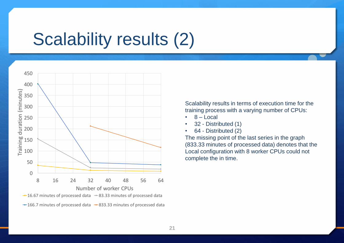
Scalability results (2)

21

0

50

100

150

200

250

300

350

400

450

8 16 24 32 40 48 56 64

Trai

nin

g d

ura

tio

n (

min

ute

s)

Number of worker CPUs16.67 minutes of processed data 83.33 minutes of processed data

166.7 minutes of processed data 833.33 minutes of processed data

Scalability results in terms of execution time for the

training process with a varying number of CPUs:

• 8 – Local

• 32 - Distributed (1)

• 64 - Distributed (2)

The missing point of the last series in the graph

(833.33 minutes of processed data) denotes that the

Local configuration with 8 worker CPUs could not

complete the in time.

Conclusion

22

The results show that, overall, the proposed AE and AE-GBT

significantly outperform the competitor methods

AE-GBT significantly outperforms AE.

The AE-GBT, Conv1D and the Deep Filtering methods require labeled

data of both classes during the learning phase.

Since it is not always possible to know the morphology of the expected

phenomena, the AE approach could be a valid alternative to AE-GBT.

The proposed methods scale well using Apache Spark

Thank you