Embed Size (px)
Citation preview
Scalable Algorithms forLocally Low-Rank Matrix ModelingQilong Gu
Dept of Computer Science and EngineeringUniversity of Minnesota Twin Cities
guxxx396csumnedu
Joshua D TrzaskoDept of Radiology
Mayo ClinicTrzaskoJoshuamayoedu
Arindam BanerjeeDept of Computer Science and Engineering
University of Minnesota Twin Citiesbanerjeecsumnedu
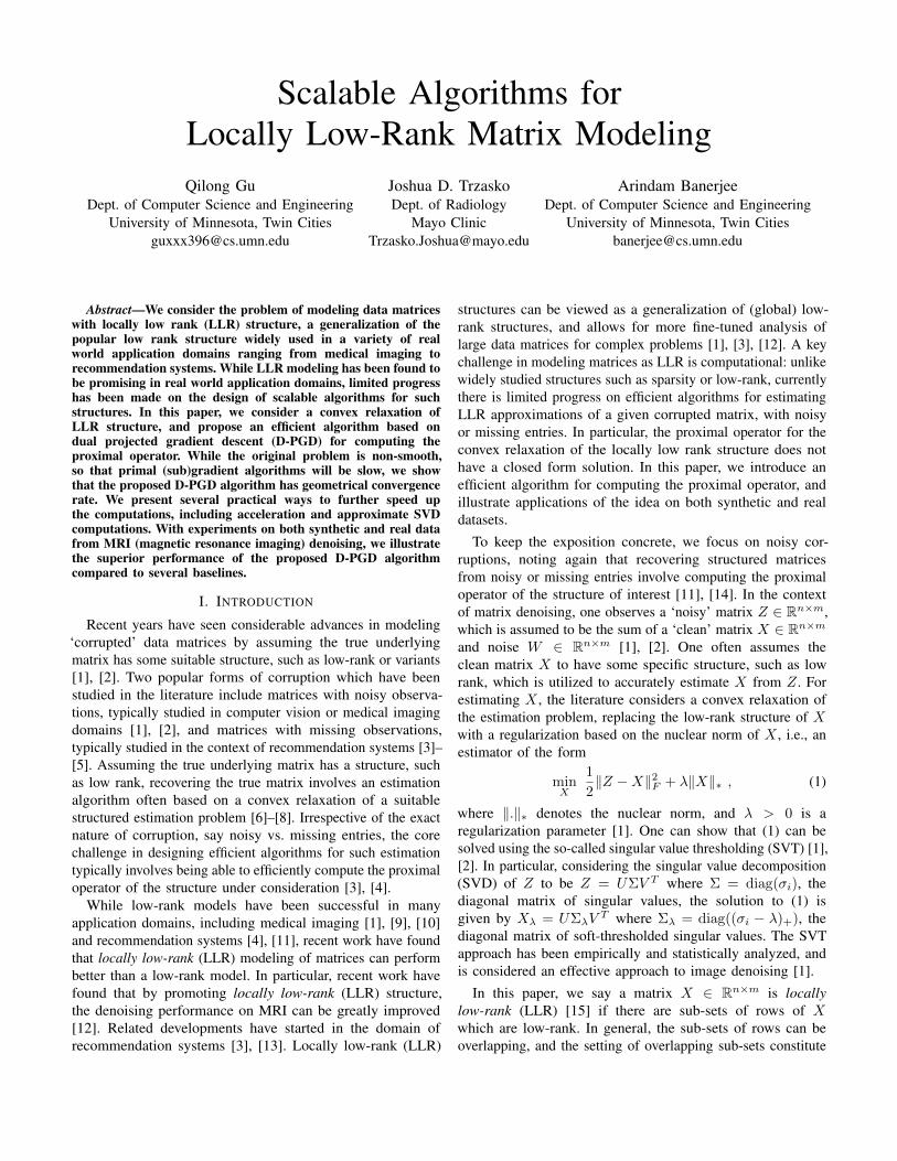
AbstractmdashWe consider the problem of modeling data matriceswith locally low rank (LLR) structure a generalization of thepopular low rank structure widely used in a variety of realworld application domains ranging from medical imaging torecommendation systems While LLR modeling has been found tobe promising in real world application domains limited progresshas been made on the design of scalable algorithms for suchstructures In this paper we consider a convex relaxation ofLLR structure and propose an efficient algorithm based ondual projected gradient descent (D-PGD) for computing theproximal operator While the original problem is non-smoothso that primal (sub)gradient algorithms will be slow we showthat the proposed D-PGD algorithm has geometrical convergencerate We present several practical ways to further speed upthe computations including acceleration and approximate SVDcomputations With experiments on both synthetic and real datafrom MRI (magnetic resonance imaging) denoising we illustratethe superior performance of the proposed D-PGD algorithmcompared to several baselines
I INTRODUCTION
Recent years have seen considerable advances in modelinglsquocorruptedrsquo data matrices by assuming the true underlyingmatrix has some suitable structure such as low-rank or variants[1] [2] Two popular forms of corruption which have beenstudied in the literature include matrices with noisy observa-tions typically studied in computer vision or medical imagingdomains [1] [2] and matrices with missing observationstypically studied in the context of recommendation systems [3]ndash[5] Assuming the true underlying matrix has a structure suchas low rank recovering the true matrix involves an estimationalgorithm often based on a convex relaxation of a suitablestructured estimation problem [6]ndash[8] Irrespective of the exactnature of corruption say noisy vs missing entries the corechallenge in designing efficient algorithms for such estimationtypically involves being able to efficiently compute the proximaloperator of the structure under consideration [3] [4]
While low-rank models have been successful in manyapplication domains including medical imaging [1] [9] [10]and recommendation systems [4] [11] recent work have foundthat locally low-rank (LLR) modeling of matrices can performbetter than a low-rank model In particular recent work havefound that by promoting locally low-rank (LLR) structurethe denoising performance on MRI can be greatly improved[12] Related developments have started in the domain ofrecommendation systems [3] [13] Locally low-rank (LLR)
structures can be viewed as a generalization of (global) low-rank structures and allows for more fine-tuned analysis oflarge data matrices for complex problems [1] [3] [12] A keychallenge in modeling matrices as LLR is computational unlikewidely studied structures such as sparsity or low-rank currentlythere is limited progress on efficient algorithms for estimatingLLR approximations of a given corrupted matrix with noisyor missing entries In particular the proximal operator for theconvex relaxation of the locally low rank structure does nothave a closed form solution In this paper we introduce anefficient algorithm for computing the proximal operator andillustrate applications of the idea on both synthetic and realdatasets
To keep the exposition concrete we focus on noisy cor-ruptions noting again that recovering structured matricesfrom noisy or missing entries involve computing the proximaloperator of the structure of interest [11] [14] In the contextof matrix denoising one observes a lsquonoisyrsquo matrix Z isin Rntimesmwhich is assumed to be the sum of a lsquocleanrsquo matrix X isin Rntimesmand noise W isin Rntimesm [1] [2] One often assumes theclean matrix X to have some specific structure such as lowrank which is utilized to accurately estimate X from Z Forestimating X the literature considers a convex relaxation ofthe estimation problem replacing the low-rank structure of Xwith a regularization based on the nuclear norm of X ie anestimator of the form
minX
1
2Z minusX2F + λXlowast (1)
where lowast denotes the nuclear norm and λ gt 0 is aregularization parameter [1] One can show that (1) can besolved using the so-called singular value thresholding (SVT) [1][2] In particular considering the singular value decomposition(SVD) of Z to be Z = UΣV T where Σ = diag(σi) thediagonal matrix of singular values the solution to (1) isgiven by Xλ = UΣλV
T where Σλ = diag((σi minus λ)+) thediagonal matrix of soft-thresholded singular values The SVTapproach has been empirically and statistically analyzed andis considered an effective approach to image denoising [1]
In this paper we say a matrix X isin Rntimesm is locallylow-rank (LLR) [15] if there are sub-sets of rows of Xwhich are low-rank In general the sub-sets of rows can beoverlapping and the setting of overlapping sub-sets constitute
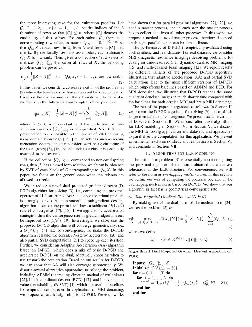
the more interesting case for the estimation problem LetGi sube 1 2 n i = 1 L be the indices of the i-th subset of rows so that |Gi| le n where |Gi| denotes thecardinality of that subset For each subset Gi there is acorresponding row-selection matrix QGi isin 0 1|Gi|timesm sothat QGiX extracts rows in Gi from X and forms a |Gi| timesmmatrix By the locally low-rank assumption each submatrixQGiX is low-rank Then given a collection of row-selectionmatrices QGiLi=1 that cover all rows of X the denoisingproblem can be posed as
minX
1
2Z minusX2F st QGiX i = 1 L are low rank
(2)In this paper we consider a convex relaxation of the problem in(2) where the low-rank structure is captured by a regularizationbased on the nuclear norm of the sub-matrices In particularwe focus on the following convex optimization problem
minX
g(X) =1
2Z minusX2F + λ
Lsumi=1
QGiXlowast (3)
where λ gt 0 is a constant and the collection of row-selection matrices QGiLi=1 is pre-specified Note that suchpre-specification is possible in the context of MRI denoisingusing domain knowledge [12] [15] In settings such as recom-mendation systems one can consider overlapping clustering ofthe users (rows) [3] [16] so that each user cluster is essentiallyassumed to be low-rank
If the collection QGiLi=1 correspond to non-overlappingrows then (3) has a closed form solution which can be obtainedby SVT of each block of Z corresponding to QGiX In thispaper we focus on the general case when the subsets areallowed to overlap
We introduce a novel dual projected gradient descent (D-PGD) algorithm for solving (3) ie computing the proximaloperator of LLR structures Note that since the primal problemis strongly convex but non-smooth a sub-gradient descentalgorithm based on the primal will have a sublinear O(1
radict)
rate of convergence [17] [18] If we apply some accelerationstrategies then the convergence rate of gradient algorithm canbe improved to O(1t2) [19] Interestingly we show that theproposed D-PGD algorithm will converge geometrically iea O(γt) γ lt 1 rate of convergence To make the D-PGDalgorithm scalable we consider Nesterov acceleration [20] andalso partial SVD computations [21] to speed up each iterationFurther we consider an Adaptive Acceleration (AA) algorithmbased on D-PGD which does a mix of basic D-PGD andaccelerated D-PGD on the dual adaptively choosing when touse (restart) the acceleration Based on our results for D-PGDwe can show that AA will also converge geometrically Wediscuss several alternative approaches to solving the problemincluding ADMM (alternating direction method of multipliers)[22] block coordinate descent (BCD) [17] and block singularvalue theresholding (B-SVT) [1] which are used as baselinesfor empirical comparison In application of MRI denoisingwe propose a parallel algorithm for D-PGD Previous works
have shown that for parallel proximal algorithm [22] [23] weneed a master process and in each step the master processhas to collect data from all other processes In this work wepropose a method to avoid master process therefore the speedup thought parallelization can be almost linear
The performance of D-PGD is empirically evaluated usingboth synthetic and real datasets For real datasets we considerMRI (magnetic resonance imaging) denoising problems fo-cusing on time-resolved (ie dynamic) cardiac MR imaging[15] and multi-channel brain imaging [12] We report resultson different variants of the proposed D-PGD algorithmillustrating that adaptive acceleration (AA) and partial SVDcalculations lead to the most efficient versions of D-PGDwhich outperforms baselines based on ADMM and BCD ForMRI denoising we illustrate that D-PGD reaches the samequality of denoised images in much shorter time compared withthe baselines for both cardiac MRI and brain MRI denoising
The rest of the paper is organized as follows In Section IIwe present the D-PGD algorithm for solving (3) and establishits geometrical rate of convergence We present scalable variantsof D-PGD in Section III We discuss alternative algorithmsfor LLR modeling in Section IV In Section V we discussthe MRI denoising application and datasets and approachesto parallelize the computation for this application We presentexperimental results on synthetic and real datasets in Section VIand conclude in Section VII
II ALGORITHMS FOR LLR MODELING
The estimation problem (3) is essentially about computingthe proximal operator of the norm obtained as a convexrelaxation of the LLR structure For convenience we willrefer to the norm as overlapping nuclear norm In this sectionwe outline our way of computing the proximal operator of theoverlapping nuclear norm based on D-PGD We show that ouralgorithm in fact has a geometrical convergence rate
A Dual Projected Gradient Descent (D-PGD)
By making use of the dual norm of the nuclear norm [24]we rewrite problem (3) as
minX
maxYiisinΩλi i=1L
L(X Yi) =1
2ZminusX2F+
Lsumi=1
〈QGiXYi〉
(4)where we define
Ωλi = Yi isin R|Gi|timesn Yi2 le λ (5)
Algorithm 1 Dual Projected Gradient Descent Algorithm (D-PGD)
Inputs QGiLi=1 ZInitialize Y 0
i Li=1 = 0for t = 0 1 T do
for i = 1 L doY t+1i = ΠΩλi
(Y ti minus 1dmax
QGi(sumLiprime=1Q
TGiprimeY
tiprime minus Z)))
end forend for
It is easy to verify that L(X Yi) is convex in X andconcave in Yi We can change the order of min and maxBy minimizing L(X Yi) over X and reordering we get thedual problem
minYiisinΩλi i=1L
f(YiLi=1) =1
2
∥∥∥∥∥Z minusLsumi=1
QTGiYi
∥∥∥∥∥2
F
(6)
In the dual problem (6) the overlapping part has been separatedinto different blocks We make use of projected gradient descent(PGD) [17] to solve problem (6) (Algorithm 1) Given thecurrent iterate Y ti Li=1 PGD takes a gradient step and projectsonto the feasible set as follows
Y t+1i = ΠΩλi
(Y ti minus
1
dmaxnablaf(Y ti Li=1)
) i = 1 L
(7)where the step size is determined by
dmax = maxj=1n
|i j isin Gi| (8)
the maximum number of groups a row belongs to Thedemanding aspect of the computation is a projection ontothe feasible set Ωλi and we denote the projection operator asΠΩλi
(middot) Note that for any matrix W the projection ΠΩλi(W )
can be computed exactly If the singular value decomposition ofthe matrix W = UΣV T where Σ = diag(σ(W )) and σ(W )is the vector of all singular values of W then
ΠΩλi(W ) = U diag(minσ(W ) λ)V T (9)
Note that Algorithm 1 is parameter free therefore its perfor-mance is stable
B Geometrical Convergence of D-PGD
The convergence analysis of PGD has been well studiedin the literature For general convex function and convex setΩi the convergence of algorithm is known to be sub-linearwith a O(1t) rate of convergence [25] While better rates arepossible for strongly convex and smooth functions the problem(6) is not strongly convex
Let us first characterize the optimal solution set Y =Y lowasti Li=1 of (6) A collection of variables YiLi=1 satisfy theKarush-Kuhn-Tucker (KKT) conditions of (6) if
QGi
(Z minus
Lsumiprime=1
QGiprimeYlowastiprime
)isin microipartY lowasti 2
microi(Y lowasti 2 minus λ) = 0 microi ge 0
Yi isin Ωλi i = 1 L
(10)
Since (6) is a convex optimization problem the KKT conditionsare both necessary and sufficient for optimality Note that if weintroduce a new variable Y such that Y =
sumLi=1Q
TGiYi then
the new objective function g(Y ) = 12Z minus Y
2F is strongly
convex Then using [26 Proposition 1] we can show thefollowing result
Lemma 1 For problem (6) there are a matrix Y lowast andmicroi ge 0 i = 1 L such that for all YiLi=1 isin YLsumi=1
QGiYlowasti = Y lowast QGiX
lowast isin microipartY lowasti 2 microi(Yi2minusλ) = 0
(11)where Xlowast = Z minus Y lowastLemma 1 shows that Y can be characterized by Y lowast and microiBy convex analysis we also have
Y =
YiLi=1
Lsumi=1
QTGiYi = Y lowast Yi isin λpartQGiXlowastlowast
(12)which gives alternative optimality conditions that do not requiremicroi The characterization of Y as in (12) plays an importantrole in our analysis
Our convergence analysis is based on the error boundproperty (EBP) of problem (6) Let
d(YiLi=1Y) = infY primei Li=1isinY
radicradicradicradic Lsumi=1
Yi minus Y primei 2F (13)
be the distance of any collection YiLi=1 to optimal solutionset Y Further for any collection YiLi=1 let
Ri(Yi) = ΠΩλi(Yi+QGi(Zminus
Lsumiprime=1
QGiprimeYiprime))minusYi i = 1 L
(14)which characterizes the residual corresponding to one gradientupdate of Algorithm 1
Our first key result (Theorem 2) shows that under mildconditions the EBP based characterization d(YiLi=1Y) is of
the orderradicsumL
i=1 Ri(Yi)2F for all feasible YiLi=1Theorem 2 Suppose there exists an Y lowasti Li=1 isin Y such that
λ isin σ(Y lowasti +QGiXlowast) i = 1 L (15)
so λ is not one of the singular values of (Y lowasti +QGiXlowast) Then
there exist constant κ gt 0 such that
d(YiLi=1Y) le κ
radicradicradicradic Lsumi=1
Ri(Yi)2F
for any Yi isin Ωλi i = 1 L
(16)
We present a sketch of the proof belowProof sketch The structure of our proof follows the frame-
work in [26] Let
Γ(Y ) =
YiLi=1
Lsumi=1
QTGiYi = Y
(17)
which is the solution set of a linear system It follows from(12) that the solution set Y = Γ(Y lowast) cap
otimesLi=1 λpartQGiXlowastlowast
whereotimes
is the Cartesian product If condition (15) holds thenwe can decouple the pair (Γ(Y lowast)
otimesLi=1 λpartQGiXlowastlowast) by the
following lemma
Lemma 3 Suppose there exists a Y lowasti Li=1 isin Y satisfying
λ isin σ(Y lowasti +QGiXlowast) i = 1 L
Then there exists a constant κ gt 0 such that
d(YiLi=1Y) le κ(d(YiLi=1Γ(Y lowast))+
d(YiLi=1
Lotimesi=1
partQGiXlowastlowast))(18)
By Hoffmanrsquos bound [27] there is a constant κ2 gt 0 such that
d(YiLi=1Γ(Y lowast)) le κ2Lsumi=1
QTGiYi minus YlowastF (19)
Further the second term on right hand side of (18) can bebounded by
d(YiLi=1
Lotimesi=1
λpartQGiXlowastlowast)) le κ3
radicradicradicradic Lsumi=1
Xi minusQGiXlowast2F
for all Yi isin partXilowast(20)
which follows the following bound for each blockLemma 4 For any Y lowasti such that Y lowasti isin λpartQGiXlowastlowast there
exist constants κprimei gt 0 such that
d(Yi λpartQGiXlowastlowast) le κprimeiXi minusQGiXlowastF (21)
for all matrices Yi Xi that satisfy Yi isin λpartXilowastLet κ4 = maxκ2 κ3 Replace the bounds from (19) and(20) in (18) we have
d(YiLi=1Y) leκ4(Lsumi=1
QTGiYi minus YlowastF+radicradicradicradic Lsum
i=1
Xi minusQGiXlowast2F )
for all Yi isin partXilowast
(22)
Then follows by Lemma 5Lemma 5 Suppose there is a constant κ4 gt 0 such that (22)
holds Then there exist constants κ gt 0 such that
d(YiLi=1Y) le κ
radicradicradicradic Lsumi=1
Ri(Yi)2F
for any Yi isin Ωλi i = 1 L
the error bound (16) holds
Note that the condition (15) under which the result holds ismild since one just needs to choose λ not to be a singular valueof the matrix Y lowasti +QGiX
lowast for some Y lowasti Using the EBP boundin Theorem 2 and the framework in [28] we now establishthe geometrically convergence of D-PGD in Algorithm 1
Theorem 6 Suppose there exists an Y lowasti Li=1 isin Y such that
λ isin σ(Y lowasti +QGiXlowast) i = 1 L (23)
Then the sequence f(Y ti Li=1)tge0 generated by Algorithm
1 converge to the optimal value flowast and there is a constantη isin (0 1) such that all t ge 0 satisfies
f(Y t+1i Li=1)minus flowast le η
η + 1(f(Y ti Li=1)minus flowast) (24)
We present a sketch of the proof belowProof sketch By our assumption and the following lemmas
Lemma 7 For every Yi function
gi(s) =1
sYi minusΠΩλi
(Yi minus snablafi(Yi))F s gt 0
is monotonically nonincreasingLemma 8 The sequence f(Y ti Li=1)tge0 generated by
PGD (1) satisfies
f(Y t+1i Li=1)minus flowast le dmax
radicradicradicradic Lsum
i=1
Y ti minus Yt+1i 2F+
radicradicradicradic Lsumi=1
Y ti minus Y lowasti 2F
radicradicradicradic Lsum
i=1
Y ti minus Yt+1i 2F
(25)we have
f(Y t+1i Li=1)minus flowast le dmax(1 + κ)
Lsumi=1
Y ti minus Y t+1i 2F (26)
We bound right hand side of (26) byLemma 9 The sequence f(Y ti Li=1)tge0 generated by
PGD (1) satisfies
f(Y ti Li=1)minus f(Y t+1i Li=1) ge dmax
2
Lsumi=1
Y ti minus Y t+1i 2F
(27)and get f(Y t+1
i Li=1) minus flowast le 2(1 + κ)(f(Y ti Li=1) minusf(Y t+1
i Li=1)) which implies
f(Y t+1i Li=1)minus flowast le η
η + 1(f(Y ti Li=1)minus flowast)
where η = 2(1 + κ)
Thus the sequence f(Y ti Li=1)tge0 in Theorem 6 convergegeometrically ie rate of convergence γt where γ = η
η+1
III SCALABLE D-PGD UPDATES
In D-PGD the projection in (9) can be computationallydemanding for large matrix W since it requires the full SVD ofmatrix W In this section we propose a few practical strategiesto speed up the algorithm including efficiently computingthe projection operator using adaptive fixed rank SVD [21]doing Nesterov acceleration [18] [20] and doing adaptiveacceleration
A Efficient Projection using Partial SVD
Recall that for a proper convex function f itsproximal operator is defined as [25] proxf (W ) =argminU
12W minus U
2F + f(U)
Let flowast be the convex
conjugate of f the Moreau decomposition [25] [29] gives
W = proxf (W ) + proxflowast(W ) For our algorithm we knowthat the convex conjugate of indicator function IΩi(W ) isλWlowast and we can compute the projection as
ΠΩi(W ) = W minus proxλlowast(W ) (28)
Note that the proximal operator in the rhs of (28) involvesSVT To speed up the computation in practice one can doadaptive fixed rank SVD decompositions say rank svti forthe i-th block and step t and adjusting the rank for the nextiteration based on [21 Section 3]
svt+1i =
svpti +1 svpti lt svtimin(svpti + round(005|Gi| |Gi|)) svpti = svti
(29)where svpti is the number of singular values in the svti singularvalues that are larger than λ
B Acceleration Scheme
We apply Nesterovrsquos acceleration scheme introduced in [18][20] The scheme introduced a combination coefficient θt Start-
ing from 0 this coefficient is given by θt+1 =1+radic
1+4(θt)2
2 In each update in addition to pure gradient update the outputis given by a combination Y t+1
i = Y t+1i + θtminus1
θt+1 (Y t+1i minus Y ti )
where Y t+1i and Y ti are gradient updates It is unclear if this
algorithm will have a linear convergence rate Therefore wecan consider a hybrid strategy which after a few steps ofNesterov update considers a basic gradient update if thatleads to a lower objective One way to determine whichupdate rule we should use is by adaptive restarting Basedon [30] in each step we obtain both the gradient updateand the accelerated update We compare the objective valueand decide whether to do a gradient step or continue withacceleration If we choose to do pure gradient update we alsoreset the combination coefficient to 0 We refer to this methodas Adaptive Acceleration (AA)The linear convergence rateof AA is stated in Corollary 10 and follows from Theorem6 Empirical results in Section VI-A3 also shows that AAimproves over the performance of both PGD and ACC
Corollary 10 Suppose there exists an Y lowasti Li=1 isin Y suchthat condition (15) holds then algorithm AA converges linearly
IV ALTERNATIVE ALGORITHMS FOR LLR MODELING
In this section we briefly discuss three other optimizationalgorithms for LLR modeling respectively based on thealternating direction method of multiplier (ADMM) blockcoordinate descent (BCD) and blockwise singular valuethresholding (B-SVT)
A ADMM Algorithm
The optimization (3) is challenging due to the overlap of thesubsets A simple approach is to decouple the overall probleminto smaller problems corresponding to the sub-matrices and
Algorithm 2 Alternating Direction Method of Multipliers(ADMM)
Inputs QGiLi=1 Z ρ gt 0Initialize Y 0
i Li=1 = 0for t = 0 1 T do
for i = 1 L doXt+1i = argminXi
12QΩλi
Xt +Y ti minusXi2F + λρXilowast
end forXt+1 = (I + ρ
sumLi=1Q
Ti Qi)
minus1(Z + ρsumLi=1Q
Ti X
ti minus
ρsumLi=1Q
Ti Y
ti )
Y t+1i = Y ti + (QGiX minusXi)
end for
iteratively solve the smaller subproblems A direct decouplingreformulation of (3) is
minXXiLi=1
1
2Z minusX2F + λ
Lsumi=1
Xilowast st QGiX = Xi
(30)which can be solved using the Alternating Direction Methodof Multipliers (ADMM) [22] The main steps of ADMM aretwo primal steps
Xt+1i = argminXi
1
2QΩiX
t + Y ti minusXi2F +λ
ρXilowast
i = 1 L
Xt+1 = (I + ρ
Lsumi=1
QTi Qi)minus1(Z + ρ
Lsumi=1
QTi Xti minus ρ
Lsumi=1
QTi Yti )
and a dual step Y t+1i = Y ti +(QGiXminusXi) The matrix inverse
in the Xt+1 can be pre-computed The updates for Xt+1i can
be solved using SVT as discussed in Section I but can be slowif the sub-matrices are large However the Xt+1
i updates canin principle be done in parallel over i = 1 L One needsto choose the parameter ρ gt 0 and in practice the convergencecan vary based on this choice The ADMM algorithm is givenby Algorithm 2
B BCD Algorithm
For dual problem (6) instead of updating all blocks at thesame time like DPGD we can only update one or severalblocks We fixed the other blocks and minimizing the objectivefunction with respect to the chosen blocks The BCD algorithmis given by Algorithm 3
C B-SVT Algorithm
BSVT [1] is another method for denoising In BSVT wefirst solve singular value thresholding on each block
minXGi
1
2QGiZ minusXGi2F + dmaxλXGilowast (31)
then we take the average of all solutions
X =1
dmaxQTGiXGi (32)
Algorithm 3 Block Coordinate Descent (BCD)
Inputs QGiLi=1 ZInitialize Y 0
i Li=1 = 0 θ0 = 0 and choose a step sizeρ gt 0for t = 0 1 T do
choose some blocks Btfor i = 1 L do
if i isin Bt thenY t+1i = ΠΩλi
(Y ti minus ρ middotQGi(sumLiprime=1Q
TGiprimeY
tiprime minus Z)))
elseY t+1i = Y ti
end ifend for
end for
BSVT is a one pass algorithm therefore we do not neediterations
V APPLICATION MRI DENOISING
In this section we consider an important real world applica-tion for LLR modeling Magnetic Resonance Imaging (MRI)denoising The proposed algorithms were applied to locally lowrank image denoising for both time-resolved (ie dynamic)cardiac MR imaging [15] and multi-channel brain imaging[12] two applications where locally low rank-based processingtechniques have proven beneficial We briefly discuss thedatasets and also how to make use of parallel updates andBCD in these applicationsCardiac MRI The first data set tested represents a first passmyocardial perfusion cardiac MRI exam performed at 30T using a standard gradient-recalled echo (GRE) acquisitionsequence wherein imaging was continuously performed fol-lowing intravascular contrast administration to observe Insuch cases image quality (ie SNR) is typically sacrificedin exchange for high spatiotemporal resolution The secondand third data sets represent short- and long axis cine cardiacexams acquired using a 2D balanced steady state free precession(bSSFP) sequence at 15 T Due to RF specific absorption ratio(SAR) limitations cine cardiac imaging is often performed atlower field strengths which in turn limits the amount of signalgenerated during the scan For these data sets the auxiliary non-spatial dimension considered for locally low rank processingwas time For additional details about these time-resolvedcardiac data sets see [1] [9]Brain MRI The proposed algorithms were also tested ontwo T1-weighted brain image data sets obtained using a T1-weighted 3D spoiled gradient echo (SPGR) sequence with an 8-channel phased array receiver and RF flip angle of θ = 25 Forthese data sets the auxiliary non-spatial dimension consideredfor locally low rank processing was receiver channel indexFor additional details about these multi-channel data sets see[31]Formulation Consider a series of T frames of NxtimesNy 2D MRimages in complex number To apply local low rank model wefirst transform it into a NxNytimesT Casorati matrix Z = Xlowast+W
Fig 1 In our parallel implementation we only decomposealong the rows of the image In this picture we want to denoisethe image on the left hand side using 4 cores so we firstdecompose it like the right hand side
Denote Gij an image block indexed by (i j) and the size ofGij is BtimesB In MR series Gij starts from the pixel located at(i j) and extends to the i+B-th column and the j+B-th rowOperator QGij extracts a B2times T submatrix from Z with rowscorresponding to block Gij in the series In our application forMRI we construct a block for each pixel in the MR image byusing cyclic way
Parallel Updates for MRI We designed a parallel D-PGDalgorithm to work in a distributed memory environment Inprevious works for parallel proximal algorithm one needs anall reduce operation in each step [22] [23] In this work wepropose a decomposition method for MRI to avoid the allreduce operation in our parallel implementation therefore thespeed up through parallelization can be almost linear Ourdecomposition method makes use of structure specific to MRimages to reduce the overhead
From our algorithm 1 update of dual variable Yij corre-sponding to block Gij is given by
Y t+1ij = ΠΩλij
(Y tij minus ρ middotQGij (sumij
QTGijYtij minus Z))) (33)
In a parallel algorithm of update (33) communication betweencores is required when computing
sumij Q
TGijY
tij and we need
all blocks to get it However in our application we onlyneed QGij
sumij Q
TGijY
tij Therefore we can merely computesum
GiprimejprimecapGij 6=emptyQTGiprimejprimeY
tiprimejprime in one core and communicate Yij
overlapping with other cores
In our algorithm we decompose the image along the rows(see figure 1) so that there will be no communication alongrows indexed by j Denote
sumij Q
TGijY
tij by Ht Suppose we
have P cores In the p-th core (p = 1 P ) we store row(pminus 1) middot NxP + 1 to row p middot NxP +B minus 1 of Ht and denote thissubmatrix as Ht
p We can compute all Y t+1ij with i indexed by
(pminus 1) middot NxP + 1 through p middot NxP using Htp Then in core p we
introduce a matrix Gt+1p and we update it locally by
Gt+1p =
pmiddotNxPsumi=(pminus1)middotNxP +1
sumj
QTGijYtij
Notice that Gt+1p 6= Ht+1
p since in the first and last B minus 1rows of Gt+1
p we need to add Y t+1 from core pminus 1 and core
p+ 1 By using matrix Gt+1p we can simply do this by
Ht+1p (1 Bminus1 ) = Gt+1
p (1 Bminus1 )+Gt+1pminus1(
NxPminusB+1
NxP )
where for a matrix A we denote A(i j ) as a submatrixextracted from the i-th to the j-th rows of each frame ofcorresponding MR series We do this by sending Gt+1
pminus1(NxP minusB + 1 NxP ) to the p-th core and the send operation can bedone from all cores in parallel Then we get the last B minus 1rows of Ht+1
p by
Ht+1p (
NxPminusB + 1
NxP ) = Ht+1
p+1(1 B minus 1 )
We only need to send Ht+1p+1(1 B minus 1 ) to the p-th core for
all possible p in parallel In our algorithm the overlapping parthas memory continuity and we have no pain manipulating suchdata In theory the speed up of our parallel implementationwill be linear
Another method we can apply to MRI series is blockcoordinate descent (BCD) One way to do this is to randomlychoose some blocks and do gradient descent on these blocksHowever this does not work for our application because it hastoo many blocks If the number of blocks we choose is smallthen it will take too many steps to update and too long to extractthese blocks Our method here is to first divide the 2D matrixinto many non-overlapping blocks In other words for any twoblocks Gi and Gj in this update we have Gi cap Gj = empty Weupdate these blocks in parallel In the next step we modify ourprevious division into blocks work with new non-overlappingblocks and do another update The process continues till allblocks have been updated In this way we can make the parallelupdates communication efficient
VI EXPERIMENTAL RESULTS
In this section we focus on experiments to illustrate theefficiency of our algorithms We do a comparison of differentalgorithms on synthetic matrices of different sizes
A Synthetic Data
We fix n = 3000 and choose m = 1000 m = 3000 andm = 5000 We use a sliding window of 1000 adjacent rowsand stepsize 250 so that the set of row subsets with low rankare
G =1 1000 251 1250 (J + 1)modm
(J + 1000)modm
where J = 250(|G| minus 1) We sample the local low-rank matrixin a hierarchically way and each low rank matrix is generatedin the same way as [25] 1 We first sample a rank 2 matrix X1
of size ntimesm then we sample a rank 1 matrix X(j)2 on each
small block of size 250 timesm for j = 1 |G| At last we
1httpstanfordedu~boydpapersprox_algsmatrix_decomphtml
time (s)
0 5000 10000
ob
jecti
ve (
log
)
-10
-5
0
5
10n = 5000
full SVD
partial SVD
time (s)
0 5000 10000
resid
ual (l
og
)
-6
-4
-2
0
2
4n = 5000
full SVD
partial SVD
Fig 2 Comparison of full SVD PGD and partial SVD PGDin computational timewhen n = 5000 Both algorithm use thesame number of iterations and converge linearly We can seethat Partial SVD based D-PGD uses considerably less time
sample a rank 1 matrix XGi on each group for i = 1 |G|Matrix Xlowast is the sum up of all the samples that is
Xlowast = X1 +
X
(1)2
X(|G|)2
+QTG1XG1 + +QTG|G|XGG (34)
The rank of each block Gi is thus less that 10 We sample anoise matrix E with iid entries from a Gaussian distributionand generate the output from Z = Xlowast + σradic
m+radicnE where σ
is the standard deviation1) Setup In our experiment we set λ = σ
dmax We use the
Frobenius norm εt = Xt minusXlowastF to measure the closenessof Xt to Xlowast where Xt = Z minus
sumLi=1Q
TGiY
ti and Xlowast is the
ldquooptimal solution to problem (3) after running algorithm AAfor a long time In our experiment we stop our algorithmwhen absolute error is less than 10minus5 We also comparethe convergence behavior of primal objective function errorg(Xt)minus g(Xlowast) For ADMM stepsize ρ is chosen to be 1
dmax
and only full SVD is used This experiment is performed oncore i7-6700 4 cores with 16 GB memory our program isimplemented using Matlab
2) Effect of Partial SVD In this experiment we test theperformance of partial SVD on synthetic data Figure 2 showsthe convergence and running time of D-PGD using partialSVD and full SVD when n = 5000 Both algorithms stop aftersimilar number of iterations However we can see that D-PGDwith partial SVD considerably outperforms D-PGD with fullSVD in terms of actual running time
3) Performance Comparison In this experiment we com-pare the performance of different algorithms on synthetic dataWe use partial SVD for D-PGD ACC and AA From Figure3 we see that D-PGD ACC and ADMM take similar numberof iterations to converge Interestingly ACC has similar orsometimes worse behavior compared to D-PGD and ADMMin terms of number of iterations and worse than D-PGD interms of time ADMM looks bad in terms of time but thatcan be attributed to ADMM using full SVD Interestingly theAA algorithm outperforms all the others both in number ofiterations and running time
B Sequential Deonising
In this experiment we apply our algorithm to denoisingdynamic cardiac MRI series and brain image The size of ourdataset is given in table (I) We have three cardiac dataset
time (s)
0 2000 4000 6000
obje
ctiv
e (lo
g)
-10
-5
0
5
10n = 5000
PGD
ACC
AA
ADMM
time (s)
0 2000 4000 6000
resi
dual
(log
)
-6
-4
-2
0
2
4n = 5000
PGD
ACC
AA
ADMM
(a) n = 5000 time (s)
0 2000 4000
obje
ctiv
e (lo
g)
-10
-5
0
5
10n = 3000
PGD
ACC
AA
ADMM
time (s)
0 2000 4000
resi
dual
(log
)
-6
-4
-2
0
2
4n = 3000
PGD
ACC
AA
ADMM
(b) n = 3000Fig 3 Comparison of PGD ACC AA and ADMM in terms of number of iterations and computational time when n = 5000and n = 3000 All algorithms converge linearly AA is the fastest algorithm in running time
0 50 100 150 200 250
time (sec)
10-4
10-2
100
102
ADMM
DPGD
BCD
(a) invivo_perfusion
0 1000 2000 3000
time (sec)
100
105ADMM
DPGD
BCD
(b) short_axis_cine
0 1000 2000 3000
time (sec)
100
102
104
ADMM
DPGD
BCD
(c) long_axis_cine
0 500 1000
time (sec)
105
ADMM
DPGD
BCD
(d) brain imaging 1
0 200 400 600 800
time (sec)
100
102
104
ADMM
DPGD
BCD
(e) brain imaging 2Fig 4 Comparison of ADMM DPDG and BCD in terms of computational time on different dataset We can see that on alldatasets DPGD outperforms other algorithms
Dataset Nx Ny Nc Tinvivo_perfusion 90 90 1 30
short_axis 144 192 8 19long_axis 192 192 8 19
brain imaging 1 256 256 8 1brain imaging 2 256 256 8 1
TABLE I Size of different set
invivo perfusion short axis and long axis The other twodatasets are brain imaging dataset
1) Setup We compare the speed of the three algorithmsADMM DPGD with adaptive acceleration and PGD Wefirst run our DPGD algorithm for a very long time to getan ldquooptimalrdquo solution Xlowast then we compare the immediateresult of each iteration of our algorithms to Xlowast Parameterλ is given by ldquocross validationrdquo we run our algorithm usingdifferent λ and the best λ is chosen by experts by looking atthe denoised images The best λ we get are invivo_perfusion005 short_axis 20 long_axis 1 brain imaging 1 25 brainimaging 2 10 We choose block size B to be 5 for all datasetFor ADMM we choose its step size ρ to be 1
dmax For BCD
we choose its step size ρ to be 1 We run ADMM and DPGDfor 100 iterations and BCD for 200 iterations This experimentis performed on core i7-6700 4 cores with 16 GB memoryour program is implemented using Matlab
2) Performance Comparison We plot running time opti-mization error XtminusXlowast2 of different algorithms We presentour plot in figure 4 in this plot XtminusXlowast2 is in log scale Fromfigure 4 we can see that all three algorithms converge linearlyThe plot also shows the efficiency of the three algorithmsBCD takes much less time for each iteration but it is not asgood as DPGD Besides the BCD curve oscillate while goingdown The performance of Vanilla ADMM is not as good Ouralgorithm is the most efficient among the three algorithms
3) Effect of Our Algorithm We make use of the result insection (VI-B2) and show the quality of denoised images For
Noisy Image LLR Denoised ADMM
LLR Denoised DPGD LLR Denoised BCD
(a) brain imaging 1
Noisy Image LLR Denoised ADMM
LLR Denoised DPGD LLR Denoised BCD
(b) brain imaging 2Fig 5 Comparison of denoised images using using ADMMDPGD with adaptive acceleration and BCD in Brain ImagingOriginal noisy images (upper left) Denoised images usingADMM (upper right) Denoised images using DPGD (bottomleft) Denoised images using BCD (bottom right)
cardiac MRI series we choose one frame from each of themThe result is presented as figure 6 For braining imaging datawe show both of them The result is presented as figure 5From these results we can see that the denoised image becomeclearer than the noisy image We also know from the result in(VI-B2) that to reach the same denoising quality DPGD takesless time than ADMM and BCD
4) Comparison with BSVT We compare LLR denoisingwith BSVT Our result is presented as Figure 7 In figure 7 weshow one frame from each cardiac MRI series and visualizationof two brain imaging datasets In the top row we show thenoisy image without denoising in the middle we show thedenoising result of BSV T and in the last row we show thedenoising result of locally low rank As BSVT is a heuristicalgorithm it is not guaranteed to solve the locally low-rankproblem Besides DPGD can be applied to problems withmissing values
C Parallel Denoising
In this experiment we apply parallel update for DPGD tothe same dataset in section (VI-B) We show show the speedup of our algorithm giving increasing number of cores
Noisy Image LLR Denoised ADMM
LLR Denoised DPGD LLR Denoised BCD
(a) invivo_perfusion
Noisy Image LLR Denoised ADMM
LLR Denoised DPGD LLR Denoised BCD
(b) short_axis
Noisy Image LLR Denoised ADMM
LLR Denoised DPGD LLR Denoised BCD
(c) long_axisFig 6 Comparison of denoised frames using ADMM DPGD with adaptive acceleration and BCD in cardiac MRI Originalnoisy images (upper left) Denoised images using ADMM (upper right) Denoised images using DPGD (bottom left) Denoisedimages using BCD (bottom right)
Noisy Image
B-SVT Denoised
LLR Denoised
(a) invivo_perfusion
Noisy Image
B-SVT Denoised
LLR Denoised
(b) short_axis
Noisy Image
B-SVT Denoised
LLR Denoised
(c) long_axis
Noisy Image
B-SVT Denoised
LLR Denoised
(d) brain imaging 1
Noisy Image
B-SVT Denoised
LLR Denoised
(e) brain imaging 2Fig 7 Comparison of BSVT denoised image and LLR denoised image Original images (top) Denoised images using BSVT(middle) Denoised images using LLR (bottom)
1) Setup We implemented a parallel version of DPGDalgorithm with adaptive acceleration using C Open BLAS andOpen MPI We run our code on a node with 32 cores providedby Intel Haswell E5-2680v3 processors and 16 GB memoryIn each run we update 50 iterations
2) Effect of Parallel Update We present our result in figure(8) In this figure the top row shows the plot of running timeversus number of cores while the row below shows the plot ofspeed up versus number cores In the top figures the blue circlesare the number of cores that we used In the figures below thered line is the ideal speed up that the speed up is the sameas number of cores From these figures we can see that thespeedup of our algorithm is almost linear with the number ofcores This accord with our discussion in section (V) becausecommunication time should not change with number of cores
VII CONCLUSIONS
In this paper we considered the locally low rank (LLR)matrix denoising problem and proposed an efficient algorithmD-PGD for solving the problem Even though the formulation isnot strongly convex we proved that D-PGD converges linearlyunder mild assumptions We introduced strategies to speed
up the algorithms in practice and illustrated performance onsynthetic and real data Applications of the LLR formulationfor missing data reconstruction will be investigated in futurework
ACKNOWLEDGMENTS
The research was supported by NSF grants IIS-1447566 IIS-1422557 CCF-1451986 CNS-1314560 IIS-0953274 IIS-1029711 NASA grant NNX12AQ39A NSFCCFCIFSmall1318347 and ldquoMayo Clinic Discovery Transla-tion Programrdquo
REFERENCES
[1] E J Candegraves C A Sing-long and J D Trzasko ldquoUnbiased RiskEstimates for Singular Value Thresholding and Spectral EstimatorsrdquoIEEE Transactions on Signal Processing vol 61 no 19 pp 4643ndash46572013
[2] D Donoho and M Gavish ldquoMinimax risk of matrix denoising by singularvalue thresholdingrdquo Annals of Statistics vol 42 no 6 pp 2413ndash24402014
[3] J Lee S Kim G Lebanon Y Singer and S Bengio ldquoLlorma Locallow-rank matrix approximationrdquo Journal of Machine Learning Researchvol 17 no 15 pp 1ndash24 2016
[4] E J Candegraves and B Recht ldquoExact matrix completion via convexoptimizationrdquo Foundations of Computational Mathematics vol 9 no 6pp 717ndash772 2009
100
101
102
number of cores
102
103
104
tim
e (
se
c)
100
101
102
number of cores
102
103
104
tim
e (
se
c)
100
101
102
number of cores
102
103
104
tim
e (
se
c)
100
101
102
number of cores
101
102
103
tim
e (
se
c)
100
101
102
number of cores
101
102
103
tim
e (
se
c)
0 5 10 15 20
number of cores
0
5
10
15
20
sp
eed
up
Total Runtime
Ideal
(a) invivo_perfusion
0 5 10 15 20 25
number of cores
0
5
10
15
20
25
sp
eed
up
Total Runtime
Ideal
(b) short_axis
0 10 20 30 40
number of cores
0
10
20
30
40
sp
eed
up
Total Runtime
Ideal
(c) long_axis
0 10 20 30 40
number of cores
0
10
20
30
40
sp
eed
up
Total Runtime
Ideal
(d) brain imaging 1
0 10 20 30 40
number of cores
0
10
20
30
40
sp
eed
up
Total Runtime
Ideal
(e) brain imaging 2Fig 8 Running time of parallel DPGD using different number of cores (top) Almost linear speed up in the number of cores(down)
[5] S Gunasekar A Banerjee and J Ghosh ldquoUnified view of matrixcompletion under general structural constraintsrdquo in Advances in NeuralInformation Processing Systems 28 2015 pp 1180ndash1188
[6] S Negahban and M J Wainwright ldquoEstimation of (near) low-rankmatrices with noise and high-dimensional scalingrdquo The Annals ofStatistics vol 39 no 2 pp 1069ndash1097 Apr 2011
[7] S Chen and A Banerjee ldquoStructured matrix recovery via thegeneralized dantzig selectorrdquo in Advances in Neural InformationProcessing Systems 29 D D Lee M Sugiyama U V LuxburgI Guyon and R Garnett Eds Curran Associates Inc 2016pp 3252ndash3260 [Online] Available httppapersnipsccpaper6394-structured-matrix-recovery-via-the-generalized-dantzig-selectorpdf
[8] A Banerjee S Chen F Fazayeli and V Sivakumar ldquoEstimation withNorm Regularizationrdquo in Advances in Neural Information ProcessingSystems 2014
[9] S Goud Y Hu and M Jacob ldquoReal-time cardiac MRI using low-rankand sparsity penaltiesrdquo in ISBI 2010 pp 988ndash991
[10] J P Haldar and Z-P Liang ldquoSpatiotemporal imaging with partiallyseparable functions A matrix recovery approachrdquo in ISBI 2010 pp716ndash719
[11] J-F Cai E J Candegraves and Z Shen ldquoA singular value thresholdingalgorithm for matrix completionrdquo SIAM Journal on Optimization vol 20no 4 pp 1956ndash1982 2010
[12] J D Trzasko and A Manduca ldquoCalibrationless parallel mri using clearrdquoin 2011 Conference Record of the Forty Fifth Asilomar Conference onSignals Systems and Computers (ASILOMAR) Nov 2011 pp 75ndash79
[13] Q Yao and J T Kwok ldquoColorization by patch-based local low-rank matrix completionrdquo in Proceedings of the Twenty-Ninth AAAIConference on Artificial Intelligence ser AAAIrsquo15 AAAI Press 2015pp 1959ndash1965 [Online] Available httpdlacmorgcitationcfmid=28865212886593
[14] S Ma D Goldfarb and L Chen ldquoFixed point and bregmaniterative methods for matrix rank minimizationrdquo MathematicalProgramming vol 128 no 1 pp 321ndash353 2011 [Online] Availablehttpdxdoiorg101007s10107-009-0306-5
[15] J D Trzasko ldquoExploiting local low-rank structure in higher-dimensionalmri applicationsrdquo pp 885 821ndash885 821ndash8 2013
[16] Y Koren ldquoFactorization meets the neighborhood A multifacetedcollaborative filtering modelrdquo in Proceedings of the 14th ACM SIGKDDInternational Conference on Knowledge Discovery and Data Mining2008 pp 426ndash434
[17] D P Bertsekas Nonlinear Programming Athena Scientific 1999[18] Y Nesterov Introductory lectures on convex optimization a basic
course ser Applied optimization Boston Dordrecht London KluwerAcademic Publ 2004
[19] K-C Toh and S Yun ldquoAn accelerated proximal gradient algorithm fornuclear norm regularized linear least squares problemsrdquo Pacific Journalof Optimization 2010 [Online] Available httpwwwmathnusedusg~mattohkcpapersmc11pdf
[20] A Beck and M Teboulle ldquoA fast iterative shrinkage-thresholdingalgorithm for linear inverse problemsrdquo SIAM Journal on ImagingSciences vol 2 no 1 pp 183ndash202 2009 [Online] Availablehttpdxdoiorg101137080716542
[21] Z Lin R Liu and Z Su ldquoLinearized Alternating Direction Methodwith Adaptive Penalty for Low-Rank Representationrdquo in Advancesin Neural Information Processing Systems 24 no 1 2011 pp 1ndash9[Online] Available httparxivorgabs11090367
[22] S Boyd N Parikh E Chu B Peleato and J Eckstein ldquoDistributedOptimization and Statistical Learning via the Alternating DirectionMethod of Multipliersrdquo Foundations and Trends in Machine Learningvol 3 no 1 pp 1ndash122 2010
[23] Z Peng M Yan and W Yin ldquoParallel and distributed sparse optimiza-tionrdquo in 2013 Asilomar Conference on Signals Systems and ComputersNov 2013 pp 659ndash646
[24] B Recht M Fazel and P A Parrilo ldquoGuaranteed minimum-ranksolutions of linear matrix equations via nuclear norm minimizationrdquoSIAM Review vol 52 no 3 pp 471ndash501 2010 [Online] Availablehttpsdoiorg101137070697835
[25] N Parikh and S Boyd ldquoProximal algorithmsrdquo Foundations and Trendsin Optimization vol 1 no 3 pp 127ndash239 2014
[26] Z Zhou and A M-C So ldquoA Unified Approach to Error Boundsfor Structured Convex Optimization Problemsrdquo arXiv151203518pp 1ndash32 2015 [Online] Available httparxivorgabs151203518$delimiter026E30F$nhttpwwwarxivorgpdf151203518pdf
[27] A J Hoffman ldquo On Approximate Solutions of Systems of LinearInequalitiesrdquo Journal of Research of the National Bureau of Standardsvol 49 no 4 pp 263ndash265 1952
[28] Z Q Luo and P Tseng ldquoError bounds and convergence analysis offeasible descent methods a general approachrdquo Annals of OperationsResearch vol 46-47 no 1 pp 157ndash178 1993
[29] J J Moreau ldquoDecomposition orthogonale drsquoun espace hilbertien selondeux cones mutuellement polairesrdquo Comptes Rendus de lrsquoAcadeacutemie desSciences vol 255 pp 238ndash240 1962
[30] B OrsquoDonoghue and E Candeacutes ldquoAdaptive Restart for AcceleratedGradient Schemesrdquo Foundations of Computational Mathematicsvol 15 no 3 pp 715ndash732 2015 [Online] Available httpdxdoiorg101007s10208-013-9150-3
[31] J D Trzasko P M Mostardi S J Riederer and A ManducaldquoEstimating t1 from multichannel variable flip angle SPGR sequencesrdquoMagnetic Resonance in Medicine vol 69 no 6 pp 1787ndash1794 6 2013
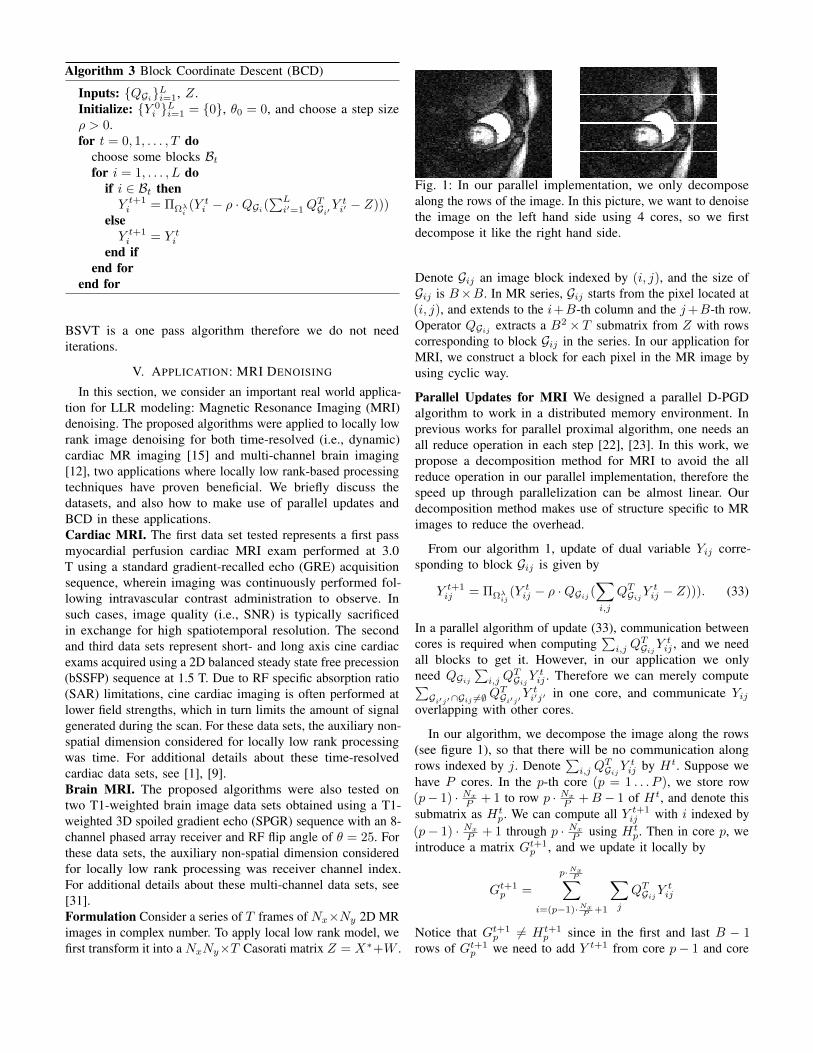
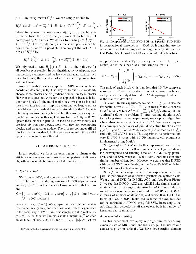
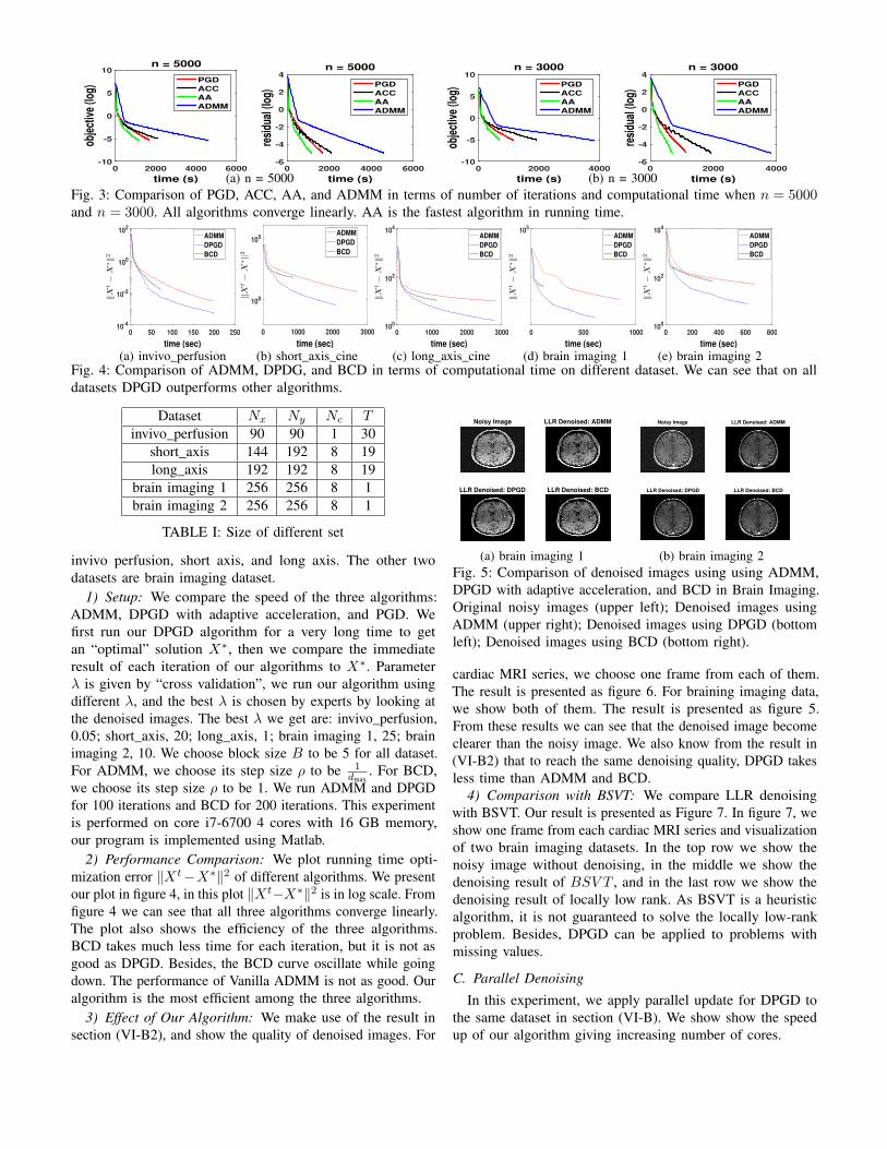
time (s)
0 2000 4000 6000
obje
ctiv
e (lo
g)
-10
-5
0
5
10n = 5000
PGD
ACC
AA
ADMM
time (s)
0 2000 4000 6000
resi
dual
(log
)
-6
-4
-2
0
2
4n = 5000
PGD
ACC
AA
ADMM
(a) n = 5000 time (s)
0 2000 4000
obje
ctiv
e (lo
g)
-10
-5
0
5
10n = 3000
PGD
ACC
AA
ADMM
time (s)
0 2000 4000
resi
dual
(log
)
-6
-4
-2
0
2
4n = 3000
PGD
ACC
AA
ADMM
(b) n = 3000Fig 3 Comparison of PGD ACC AA and ADMM in terms of number of iterations and computational time when n = 5000and n = 3000 All algorithms converge linearly AA is the fastest algorithm in running time
0 50 100 150 200 250
time (sec)
10-4
10-2
100
102
ADMM
DPGD
BCD
(a) invivo_perfusion
0 1000 2000 3000
time (sec)
100
105ADMM
DPGD
BCD
(b) short_axis_cine
0 1000 2000 3000
time (sec)
100
102
104
ADMM
DPGD
BCD
(c) long_axis_cine
0 500 1000
time (sec)
105
ADMM
DPGD
BCD
(d) brain imaging 1
0 200 400 600 800
time (sec)
100
102
104
ADMM
DPGD
BCD
(e) brain imaging 2Fig 4 Comparison of ADMM DPDG and BCD in terms of computational time on different dataset We can see that on alldatasets DPGD outperforms other algorithms
Dataset Nx Ny Nc Tinvivo_perfusion 90 90 1 30
short_axis 144 192 8 19long_axis 192 192 8 19
brain imaging 1 256 256 8 1brain imaging 2 256 256 8 1
TABLE I Size of different set
invivo perfusion short axis and long axis The other twodatasets are brain imaging dataset
1) Setup We compare the speed of the three algorithmsADMM DPGD with adaptive acceleration and PGD Wefirst run our DPGD algorithm for a very long time to getan ldquooptimalrdquo solution Xlowast then we compare the immediateresult of each iteration of our algorithms to Xlowast Parameterλ is given by ldquocross validationrdquo we run our algorithm usingdifferent λ and the best λ is chosen by experts by looking atthe denoised images The best λ we get are invivo_perfusion005 short_axis 20 long_axis 1 brain imaging 1 25 brainimaging 2 10 We choose block size B to be 5 for all datasetFor ADMM we choose its step size ρ to be 1
dmax For BCD
we choose its step size ρ to be 1 We run ADMM and DPGDfor 100 iterations and BCD for 200 iterations This experimentis performed on core i7-6700 4 cores with 16 GB memoryour program is implemented using Matlab
2) Performance Comparison We plot running time opti-mization error XtminusXlowast2 of different algorithms We presentour plot in figure 4 in this plot XtminusXlowast2 is in log scale Fromfigure 4 we can see that all three algorithms converge linearlyThe plot also shows the efficiency of the three algorithmsBCD takes much less time for each iteration but it is not asgood as DPGD Besides the BCD curve oscillate while goingdown The performance of Vanilla ADMM is not as good Ouralgorithm is the most efficient among the three algorithms
3) Effect of Our Algorithm We make use of the result insection (VI-B2) and show the quality of denoised images For
Noisy Image LLR Denoised ADMM
LLR Denoised DPGD LLR Denoised BCD
(a) brain imaging 1
Noisy Image LLR Denoised ADMM
LLR Denoised DPGD LLR Denoised BCD
(b) brain imaging 2Fig 5 Comparison of denoised images using using ADMMDPGD with adaptive acceleration and BCD in Brain ImagingOriginal noisy images (upper left) Denoised images usingADMM (upper right) Denoised images using DPGD (bottomleft) Denoised images using BCD (bottom right)
cardiac MRI series we choose one frame from each of themThe result is presented as figure 6 For braining imaging datawe show both of them The result is presented as figure 5From these results we can see that the denoised image becomeclearer than the noisy image We also know from the result in(VI-B2) that to reach the same denoising quality DPGD takesless time than ADMM and BCD
4) Comparison with BSVT We compare LLR denoisingwith BSVT Our result is presented as Figure 7 In figure 7 weshow one frame from each cardiac MRI series and visualizationof two brain imaging datasets In the top row we show thenoisy image without denoising in the middle we show thedenoising result of BSV T and in the last row we show thedenoising result of locally low rank As BSVT is a heuristicalgorithm it is not guaranteed to solve the locally low-rankproblem Besides DPGD can be applied to problems withmissing values
C Parallel Denoising
In this experiment we apply parallel update for DPGD tothe same dataset in section (VI-B) We show show the speedup of our algorithm giving increasing number of cores
Noisy Image LLR Denoised ADMM
LLR Denoised DPGD LLR Denoised BCD
(a) invivo_perfusion
Noisy Image LLR Denoised ADMM
LLR Denoised DPGD LLR Denoised BCD
(b) short_axis
Noisy Image LLR Denoised ADMM
LLR Denoised DPGD LLR Denoised BCD
(c) long_axisFig 6 Comparison of denoised frames using ADMM DPGD with adaptive acceleration and BCD in cardiac MRI Originalnoisy images (upper left) Denoised images using ADMM (upper right) Denoised images using DPGD (bottom left) Denoisedimages using BCD (bottom right)
Noisy Image
B-SVT Denoised
LLR Denoised
(a) invivo_perfusion
Noisy Image
B-SVT Denoised
LLR Denoised
(b) short_axis
Noisy Image
B-SVT Denoised
LLR Denoised
(c) long_axis
Noisy Image
B-SVT Denoised
LLR Denoised
(d) brain imaging 1
Noisy Image
B-SVT Denoised
LLR Denoised
(e) brain imaging 2Fig 7 Comparison of BSVT denoised image and LLR denoised image Original images (top) Denoised images using BSVT(middle) Denoised images using LLR (bottom)
1) Setup We implemented a parallel version of DPGDalgorithm with adaptive acceleration using C Open BLAS andOpen MPI We run our code on a node with 32 cores providedby Intel Haswell E5-2680v3 processors and 16 GB memoryIn each run we update 50 iterations
2) Effect of Parallel Update We present our result in figure(8) In this figure the top row shows the plot of running timeversus number of cores while the row below shows the plot ofspeed up versus number cores In the top figures the blue circlesare the number of cores that we used In the figures below thered line is the ideal speed up that the speed up is the sameas number of cores From these figures we can see that thespeedup of our algorithm is almost linear with the number ofcores This accord with our discussion in section (V) becausecommunication time should not change with number of cores
VII CONCLUSIONS
In this paper we considered the locally low rank (LLR)matrix denoising problem and proposed an efficient algorithmD-PGD for solving the problem Even though the formulation isnot strongly convex we proved that D-PGD converges linearlyunder mild assumptions We introduced strategies to speed
up the algorithms in practice and illustrated performance onsynthetic and real data Applications of the LLR formulationfor missing data reconstruction will be investigated in futurework
ACKNOWLEDGMENTS
The research was supported by NSF grants IIS-1447566 IIS-1422557 CCF-1451986 CNS-1314560 IIS-0953274 IIS-1029711 NASA grant NNX12AQ39A NSFCCFCIFSmall1318347 and ldquoMayo Clinic Discovery Transla-tion Programrdquo
REFERENCES
[1] E J Candegraves C A Sing-long and J D Trzasko ldquoUnbiased RiskEstimates for Singular Value Thresholding and Spectral EstimatorsrdquoIEEE Transactions on Signal Processing vol 61 no 19 pp 4643ndash46572013
[2] D Donoho and M Gavish ldquoMinimax risk of matrix denoising by singularvalue thresholdingrdquo Annals of Statistics vol 42 no 6 pp 2413ndash24402014
[3] J Lee S Kim G Lebanon Y Singer and S Bengio ldquoLlorma Locallow-rank matrix approximationrdquo Journal of Machine Learning Researchvol 17 no 15 pp 1ndash24 2016
[4] E J Candegraves and B Recht ldquoExact matrix completion via convexoptimizationrdquo Foundations of Computational Mathematics vol 9 no 6pp 717ndash772 2009
100
101
102
number of cores
102
103
104
tim
e (
se
c)
100
101
102
number of cores
102
103
104
tim
e (
se
c)
100
101
102
number of cores
102
103
104
tim
e (
se
c)
100
101
102
number of cores
101
102
103
tim
e (
se
c)
100
101
102
number of cores
101
102
103
tim
e (
se
c)
0 5 10 15 20
number of cores
0
5
10
15
20
sp
eed
up
Total Runtime
Ideal
(a) invivo_perfusion
0 5 10 15 20 25
number of cores
0
5
10
15
20
25
sp
eed
up
Total Runtime
Ideal
(b) short_axis
0 10 20 30 40
number of cores
0
10
20
30
40
sp
eed
up
Total Runtime
Ideal
(c) long_axis
0 10 20 30 40
number of cores
0
10
20
30
40
sp
eed
up
Total Runtime
Ideal
(d) brain imaging 1
0 10 20 30 40
number of cores
0
10
20
30
40
sp
eed
up
Total Runtime
Ideal
(e) brain imaging 2Fig 8 Running time of parallel DPGD using different number of cores (top) Almost linear speed up in the number of cores(down)
[5] S Gunasekar A Banerjee and J Ghosh ldquoUnified view of matrixcompletion under general structural constraintsrdquo in Advances in NeuralInformation Processing Systems 28 2015 pp 1180ndash1188
[6] S Negahban and M J Wainwright ldquoEstimation of (near) low-rankmatrices with noise and high-dimensional scalingrdquo The Annals ofStatistics vol 39 no 2 pp 1069ndash1097 Apr 2011
[7] S Chen and A Banerjee ldquoStructured matrix recovery via thegeneralized dantzig selectorrdquo in Advances in Neural InformationProcessing Systems 29 D D Lee M Sugiyama U V LuxburgI Guyon and R Garnett Eds Curran Associates Inc 2016pp 3252ndash3260 [Online] Available httppapersnipsccpaper6394-structured-matrix-recovery-via-the-generalized-dantzig-selectorpdf
[8] A Banerjee S Chen F Fazayeli and V Sivakumar ldquoEstimation withNorm Regularizationrdquo in Advances in Neural Information ProcessingSystems 2014
[9] S Goud Y Hu and M Jacob ldquoReal-time cardiac MRI using low-rankand sparsity penaltiesrdquo in ISBI 2010 pp 988ndash991
[10] J P Haldar and Z-P Liang ldquoSpatiotemporal imaging with partiallyseparable functions A matrix recovery approachrdquo in ISBI 2010 pp716ndash719
[11] J-F Cai E J Candegraves and Z Shen ldquoA singular value thresholdingalgorithm for matrix completionrdquo SIAM Journal on Optimization vol 20no 4 pp 1956ndash1982 2010
[12] J D Trzasko and A Manduca ldquoCalibrationless parallel mri using clearrdquoin 2011 Conference Record of the Forty Fifth Asilomar Conference onSignals Systems and Computers (ASILOMAR) Nov 2011 pp 75ndash79
[13] Q Yao and J T Kwok ldquoColorization by patch-based local low-rank matrix completionrdquo in Proceedings of the Twenty-Ninth AAAIConference on Artificial Intelligence ser AAAIrsquo15 AAAI Press 2015pp 1959ndash1965 [Online] Available httpdlacmorgcitationcfmid=28865212886593
[14] S Ma D Goldfarb and L Chen ldquoFixed point and bregmaniterative methods for matrix rank minimizationrdquo MathematicalProgramming vol 128 no 1 pp 321ndash353 2011 [Online] Availablehttpdxdoiorg101007s10107-009-0306-5
[15] J D Trzasko ldquoExploiting local low-rank structure in higher-dimensionalmri applicationsrdquo pp 885 821ndash885 821ndash8 2013
[16] Y Koren ldquoFactorization meets the neighborhood A multifacetedcollaborative filtering modelrdquo in Proceedings of the 14th ACM SIGKDDInternational Conference on Knowledge Discovery and Data Mining2008 pp 426ndash434
[17] D P Bertsekas Nonlinear Programming Athena Scientific 1999[18] Y Nesterov Introductory lectures on convex optimization a basic
course ser Applied optimization Boston Dordrecht London KluwerAcademic Publ 2004
[19] K-C Toh and S Yun ldquoAn accelerated proximal gradient algorithm fornuclear norm regularized linear least squares problemsrdquo Pacific Journalof Optimization 2010 [Online] Available httpwwwmathnusedusg~mattohkcpapersmc11pdf
[20] A Beck and M Teboulle ldquoA fast iterative shrinkage-thresholdingalgorithm for linear inverse problemsrdquo SIAM Journal on ImagingSciences vol 2 no 1 pp 183ndash202 2009 [Online] Availablehttpdxdoiorg101137080716542
[21] Z Lin R Liu and Z Su ldquoLinearized Alternating Direction Methodwith Adaptive Penalty for Low-Rank Representationrdquo in Advancesin Neural Information Processing Systems 24 no 1 2011 pp 1ndash9[Online] Available httparxivorgabs11090367
[22] S Boyd N Parikh E Chu B Peleato and J Eckstein ldquoDistributedOptimization and Statistical Learning via the Alternating DirectionMethod of Multipliersrdquo Foundations and Trends in Machine Learningvol 3 no 1 pp 1ndash122 2010
[23] Z Peng M Yan and W Yin ldquoParallel and distributed sparse optimiza-tionrdquo in 2013 Asilomar Conference on Signals Systems and ComputersNov 2013 pp 659ndash646
[24] B Recht M Fazel and P A Parrilo ldquoGuaranteed minimum-ranksolutions of linear matrix equations via nuclear norm minimizationrdquoSIAM Review vol 52 no 3 pp 471ndash501 2010 [Online] Availablehttpsdoiorg101137070697835
[25] N Parikh and S Boyd ldquoProximal algorithmsrdquo Foundations and Trendsin Optimization vol 1 no 3 pp 127ndash239 2014
[26] Z Zhou and A M-C So ldquoA Unified Approach to Error Boundsfor Structured Convex Optimization Problemsrdquo arXiv151203518pp 1ndash32 2015 [Online] Available httparxivorgabs151203518$delimiter026E30F$nhttpwwwarxivorgpdf151203518pdf
[27] A J Hoffman ldquo On Approximate Solutions of Systems of LinearInequalitiesrdquo Journal of Research of the National Bureau of Standardsvol 49 no 4 pp 263ndash265 1952
[28] Z Q Luo and P Tseng ldquoError bounds and convergence analysis offeasible descent methods a general approachrdquo Annals of OperationsResearch vol 46-47 no 1 pp 157ndash178 1993
[29] J J Moreau ldquoDecomposition orthogonale drsquoun espace hilbertien selondeux cones mutuellement polairesrdquo Comptes Rendus de lrsquoAcadeacutemie desSciences vol 255 pp 238ndash240 1962
[30] B OrsquoDonoghue and E Candeacutes ldquoAdaptive Restart for AcceleratedGradient Schemesrdquo Foundations of Computational Mathematicsvol 15 no 3 pp 715ndash732 2015 [Online] Available httpdxdoiorg101007s10208-013-9150-3
[31] J D Trzasko P M Mostardi S J Riederer and A ManducaldquoEstimating t1 from multichannel variable flip angle SPGR sequencesrdquoMagnetic Resonance in Medicine vol 69 no 6 pp 1787ndash1794 6 2013
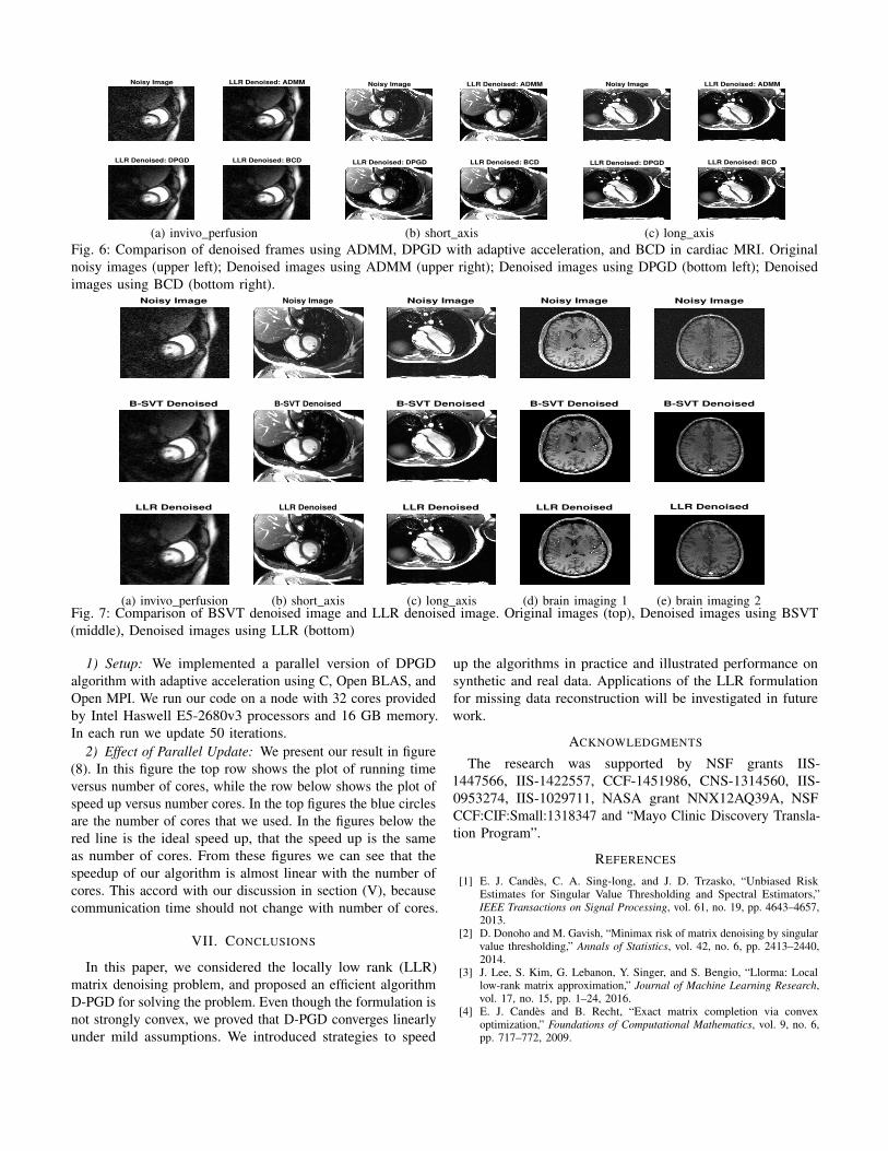
Noisy Image LLR Denoised ADMM
LLR Denoised DPGD LLR Denoised BCD
(a) invivo_perfusion
Noisy Image LLR Denoised ADMM
LLR Denoised DPGD LLR Denoised BCD
(b) short_axis
Noisy Image LLR Denoised ADMM
LLR Denoised DPGD LLR Denoised BCD
(c) long_axisFig 6 Comparison of denoised frames using ADMM DPGD with adaptive acceleration and BCD in cardiac MRI Originalnoisy images (upper left) Denoised images using ADMM (upper right) Denoised images using DPGD (bottom left) Denoisedimages using BCD (bottom right)
Noisy Image
B-SVT Denoised
LLR Denoised
(a) invivo_perfusion
Noisy Image
B-SVT Denoised
LLR Denoised
(b) short_axis
Noisy Image
B-SVT Denoised
LLR Denoised
(c) long_axis
Noisy Image
B-SVT Denoised
LLR Denoised
(d) brain imaging 1
Noisy Image
B-SVT Denoised
LLR Denoised
(e) brain imaging 2Fig 7 Comparison of BSVT denoised image and LLR denoised image Original images (top) Denoised images using BSVT(middle) Denoised images using LLR (bottom)
1) Setup We implemented a parallel version of DPGDalgorithm with adaptive acceleration using C Open BLAS andOpen MPI We run our code on a node with 32 cores providedby Intel Haswell E5-2680v3 processors and 16 GB memoryIn each run we update 50 iterations
2) Effect of Parallel Update We present our result in figure(8) In this figure the top row shows the plot of running timeversus number of cores while the row below shows the plot ofspeed up versus number cores In the top figures the blue circlesare the number of cores that we used In the figures below thered line is the ideal speed up that the speed up is the sameas number of cores From these figures we can see that thespeedup of our algorithm is almost linear with the number ofcores This accord with our discussion in section (V) becausecommunication time should not change with number of cores
VII CONCLUSIONS
In this paper we considered the locally low rank (LLR)matrix denoising problem and proposed an efficient algorithmD-PGD for solving the problem Even though the formulation isnot strongly convex we proved that D-PGD converges linearlyunder mild assumptions We introduced strategies to speed
up the algorithms in practice and illustrated performance onsynthetic and real data Applications of the LLR formulationfor missing data reconstruction will be investigated in futurework
ACKNOWLEDGMENTS
The research was supported by NSF grants IIS-1447566 IIS-1422557 CCF-1451986 CNS-1314560 IIS-0953274 IIS-1029711 NASA grant NNX12AQ39A NSFCCFCIFSmall1318347 and ldquoMayo Clinic Discovery Transla-tion Programrdquo
REFERENCES
[1] E J Candegraves C A Sing-long and J D Trzasko ldquoUnbiased RiskEstimates for Singular Value Thresholding and Spectral EstimatorsrdquoIEEE Transactions on Signal Processing vol 61 no 19 pp 4643ndash46572013
[2] D Donoho and M Gavish ldquoMinimax risk of matrix denoising by singularvalue thresholdingrdquo Annals of Statistics vol 42 no 6 pp 2413ndash24402014
[3] J Lee S Kim G Lebanon Y Singer and S Bengio ldquoLlorma Locallow-rank matrix approximationrdquo Journal of Machine Learning Researchvol 17 no 15 pp 1ndash24 2016
[4] E J Candegraves and B Recht ldquoExact matrix completion via convexoptimizationrdquo Foundations of Computational Mathematics vol 9 no 6pp 717ndash772 2009
100
101
102
number of cores
102
103
104
tim
e (
se
c)
100
101
102
number of cores
102
103
104
tim
e (
se
c)
100
101
102
number of cores
102
103
104
tim
e (
se
c)
100
101
102
number of cores
101
102
103
tim
e (
se
c)
100
101
102
number of cores
101
102
103
tim
e (
se
c)
0 5 10 15 20
number of cores
0
5
10
15
20
sp
eed
up
Total Runtime
Ideal
(a) invivo_perfusion
0 5 10 15 20 25
number of cores
0
5
10
15
20
25
sp
eed
up
Total Runtime
Ideal
(b) short_axis
0 10 20 30 40
number of cores
0
10
20
30
40
sp
eed
up
Total Runtime
Ideal
(c) long_axis
0 10 20 30 40
number of cores
0
10
20
30
40
sp
eed
up
Total Runtime
Ideal
(d) brain imaging 1
0 10 20 30 40
number of cores
0
10
20
30
40
sp
eed
up
Total Runtime
Ideal
(e) brain imaging 2Fig 8 Running time of parallel DPGD using different number of cores (top) Almost linear speed up in the number of cores(down)
[5] S Gunasekar A Banerjee and J Ghosh ldquoUnified view of matrixcompletion under general structural constraintsrdquo in Advances in NeuralInformation Processing Systems 28 2015 pp 1180ndash1188
[6] S Negahban and M J Wainwright ldquoEstimation of (near) low-rankmatrices with noise and high-dimensional scalingrdquo The Annals ofStatistics vol 39 no 2 pp 1069ndash1097 Apr 2011
[7] S Chen and A Banerjee ldquoStructured matrix recovery via thegeneralized dantzig selectorrdquo in Advances in Neural InformationProcessing Systems 29 D D Lee M Sugiyama U V LuxburgI Guyon and R Garnett Eds Curran Associates Inc 2016pp 3252ndash3260 [Online] Available httppapersnipsccpaper6394-structured-matrix-recovery-via-the-generalized-dantzig-selectorpdf
[8] A Banerjee S Chen F Fazayeli and V Sivakumar ldquoEstimation withNorm Regularizationrdquo in Advances in Neural Information ProcessingSystems 2014
[9] S Goud Y Hu and M Jacob ldquoReal-time cardiac MRI using low-rankand sparsity penaltiesrdquo in ISBI 2010 pp 988ndash991
[10] J P Haldar and Z-P Liang ldquoSpatiotemporal imaging with partiallyseparable functions A matrix recovery approachrdquo in ISBI 2010 pp716ndash719
[11] J-F Cai E J Candegraves and Z Shen ldquoA singular value thresholdingalgorithm for matrix completionrdquo SIAM Journal on Optimization vol 20no 4 pp 1956ndash1982 2010
[12] J D Trzasko and A Manduca ldquoCalibrationless parallel mri using clearrdquoin 2011 Conference Record of the Forty Fifth Asilomar Conference onSignals Systems and Computers (ASILOMAR) Nov 2011 pp 75ndash79
[13] Q Yao and J T Kwok ldquoColorization by patch-based local low-rank matrix completionrdquo in Proceedings of the Twenty-Ninth AAAIConference on Artificial Intelligence ser AAAIrsquo15 AAAI Press 2015pp 1959ndash1965 [Online] Available httpdlacmorgcitationcfmid=28865212886593
[14] S Ma D Goldfarb and L Chen ldquoFixed point and bregmaniterative methods for matrix rank minimizationrdquo MathematicalProgramming vol 128 no 1 pp 321ndash353 2011 [Online] Availablehttpdxdoiorg101007s10107-009-0306-5
[15] J D Trzasko ldquoExploiting local low-rank structure in higher-dimensionalmri applicationsrdquo pp 885 821ndash885 821ndash8 2013
[16] Y Koren ldquoFactorization meets the neighborhood A multifacetedcollaborative filtering modelrdquo in Proceedings of the 14th ACM SIGKDDInternational Conference on Knowledge Discovery and Data Mining2008 pp 426ndash434
[17] D P Bertsekas Nonlinear Programming Athena Scientific 1999[18] Y Nesterov Introductory lectures on convex optimization a basic
course ser Applied optimization Boston Dordrecht London KluwerAcademic Publ 2004
[19] K-C Toh and S Yun ldquoAn accelerated proximal gradient algorithm fornuclear norm regularized linear least squares problemsrdquo Pacific Journalof Optimization 2010 [Online] Available httpwwwmathnusedusg~mattohkcpapersmc11pdf
[20] A Beck and M Teboulle ldquoA fast iterative shrinkage-thresholdingalgorithm for linear inverse problemsrdquo SIAM Journal on ImagingSciences vol 2 no 1 pp 183ndash202 2009 [Online] Availablehttpdxdoiorg101137080716542
[21] Z Lin R Liu and Z Su ldquoLinearized Alternating Direction Methodwith Adaptive Penalty for Low-Rank Representationrdquo in Advancesin Neural Information Processing Systems 24 no 1 2011 pp 1ndash9[Online] Available httparxivorgabs11090367
[22] S Boyd N Parikh E Chu B Peleato and J Eckstein ldquoDistributedOptimization and Statistical Learning via the Alternating DirectionMethod of Multipliersrdquo Foundations and Trends in Machine Learningvol 3 no 1 pp 1ndash122 2010
[23] Z Peng M Yan and W Yin ldquoParallel and distributed sparse optimiza-tionrdquo in 2013 Asilomar Conference on Signals Systems and ComputersNov 2013 pp 659ndash646
[24] B Recht M Fazel and P A Parrilo ldquoGuaranteed minimum-ranksolutions of linear matrix equations via nuclear norm minimizationrdquoSIAM Review vol 52 no 3 pp 471ndash501 2010 [Online] Availablehttpsdoiorg101137070697835
[25] N Parikh and S Boyd ldquoProximal algorithmsrdquo Foundations and Trendsin Optimization vol 1 no 3 pp 127ndash239 2014
[26] Z Zhou and A M-C So ldquoA Unified Approach to Error Boundsfor Structured Convex Optimization Problemsrdquo arXiv151203518pp 1ndash32 2015 [Online] Available httparxivorgabs151203518$delimiter026E30F$nhttpwwwarxivorgpdf151203518pdf
[27] A J Hoffman ldquo On Approximate Solutions of Systems of LinearInequalitiesrdquo Journal of Research of the National Bureau of Standardsvol 49 no 4 pp 263ndash265 1952
[28] Z Q Luo and P Tseng ldquoError bounds and convergence analysis offeasible descent methods a general approachrdquo Annals of OperationsResearch vol 46-47 no 1 pp 157ndash178 1993
[29] J J Moreau ldquoDecomposition orthogonale drsquoun espace hilbertien selondeux cones mutuellement polairesrdquo Comptes Rendus de lrsquoAcadeacutemie desSciences vol 255 pp 238ndash240 1962
[30] B OrsquoDonoghue and E Candeacutes ldquoAdaptive Restart for AcceleratedGradient Schemesrdquo Foundations of Computational Mathematicsvol 15 no 3 pp 715ndash732 2015 [Online] Available httpdxdoiorg101007s10208-013-9150-3
[31] J D Trzasko P M Mostardi S J Riederer and A ManducaldquoEstimating t1 from multichannel variable flip angle SPGR sequencesrdquoMagnetic Resonance in Medicine vol 69 no 6 pp 1787ndash1794 6 2013
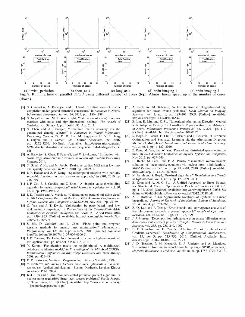
100
101
102
number of cores
102
103
104
tim
e (
se
c)
100
101
102
number of cores
102
103
104
tim
e (
se
c)
100
101
102
number of cores
102
103
104
tim
e (
se
c)
100
101
102
number of cores
101
102
103
tim
e (
se
c)
100
101
102
number of cores
101
102
103
tim
e (
se
c)
0 5 10 15 20
number of cores
0
5
10
15
20
sp
eed
up
Total Runtime
Ideal
(a) invivo_perfusion
0 5 10 15 20 25
number of cores
0
5
10
15
20
25
sp
eed
up
Total Runtime
Ideal
(b) short_axis
0 10 20 30 40
number of cores
0
10
20
30
40
sp
eed
up
Total Runtime
Ideal
(c) long_axis
0 10 20 30 40
number of cores
0
10
20
30
40
sp
eed
up
Total Runtime
Ideal
(d) brain imaging 1
0 10 20 30 40
number of cores
0
10
20
30
40
sp
eed
up
Total Runtime
Ideal
(e) brain imaging 2Fig 8 Running time of parallel DPGD using different number of cores (top) Almost linear speed up in the number of cores(down)
[5] S Gunasekar A Banerjee and J Ghosh ldquoUnified view of matrixcompletion under general structural constraintsrdquo in Advances in NeuralInformation Processing Systems 28 2015 pp 1180ndash1188
[6] S Negahban and M J Wainwright ldquoEstimation of (near) low-rankmatrices with noise and high-dimensional scalingrdquo The Annals ofStatistics vol 39 no 2 pp 1069ndash1097 Apr 2011
[7] S Chen and A Banerjee ldquoStructured matrix recovery via thegeneralized dantzig selectorrdquo in Advances in Neural InformationProcessing Systems 29 D D Lee M Sugiyama U V LuxburgI Guyon and R Garnett Eds Curran Associates Inc 2016pp 3252ndash3260 [Online] Available httppapersnipsccpaper6394-structured-matrix-recovery-via-the-generalized-dantzig-selectorpdf
[8] A Banerjee S Chen F Fazayeli and V Sivakumar ldquoEstimation withNorm Regularizationrdquo in Advances in Neural Information ProcessingSystems 2014
[9] S Goud Y Hu and M Jacob ldquoReal-time cardiac MRI using low-rankand sparsity penaltiesrdquo in ISBI 2010 pp 988ndash991
[10] J P Haldar and Z-P Liang ldquoSpatiotemporal imaging with partiallyseparable functions A matrix recovery approachrdquo in ISBI 2010 pp716ndash719
[11] J-F Cai E J Candegraves and Z Shen ldquoA singular value thresholdingalgorithm for matrix completionrdquo SIAM Journal on Optimization vol 20no 4 pp 1956ndash1982 2010
[12] J D Trzasko and A Manduca ldquoCalibrationless parallel mri using clearrdquoin 2011 Conference Record of the Forty Fifth Asilomar Conference onSignals Systems and Computers (ASILOMAR) Nov 2011 pp 75ndash79
[13] Q Yao and J T Kwok ldquoColorization by patch-based local low-rank matrix completionrdquo in Proceedings of the Twenty-Ninth AAAIConference on Artificial Intelligence ser AAAIrsquo15 AAAI Press 2015pp 1959ndash1965 [Online] Available httpdlacmorgcitationcfmid=28865212886593
[14] S Ma D Goldfarb and L Chen ldquoFixed point and bregmaniterative methods for matrix rank minimizationrdquo MathematicalProgramming vol 128 no 1 pp 321ndash353 2011 [Online] Availablehttpdxdoiorg101007s10107-009-0306-5
[15] J D Trzasko ldquoExploiting local low-rank structure in higher-dimensionalmri applicationsrdquo pp 885 821ndash885 821ndash8 2013
[16] Y Koren ldquoFactorization meets the neighborhood A multifacetedcollaborative filtering modelrdquo in Proceedings of the 14th ACM SIGKDDInternational Conference on Knowledge Discovery and Data Mining2008 pp 426ndash434
[17] D P Bertsekas Nonlinear Programming Athena Scientific 1999[18] Y Nesterov Introductory lectures on convex optimization a basic
course ser Applied optimization Boston Dordrecht London KluwerAcademic Publ 2004
[19] K-C Toh and S Yun ldquoAn accelerated proximal gradient algorithm fornuclear norm regularized linear least squares problemsrdquo Pacific Journalof Optimization 2010 [Online] Available httpwwwmathnusedusg~mattohkcpapersmc11pdf
[20] A Beck and M Teboulle ldquoA fast iterative shrinkage-thresholdingalgorithm for linear inverse problemsrdquo SIAM Journal on ImagingSciences vol 2 no 1 pp 183ndash202 2009 [Online] Availablehttpdxdoiorg101137080716542
[21] Z Lin R Liu and Z Su ldquoLinearized Alternating Direction Methodwith Adaptive Penalty for Low-Rank Representationrdquo in Advancesin Neural Information Processing Systems 24 no 1 2011 pp 1ndash9[Online] Available httparxivorgabs11090367
[22] S Boyd N Parikh E Chu B Peleato and J Eckstein ldquoDistributedOptimization and Statistical Learning via the Alternating DirectionMethod of Multipliersrdquo Foundations and Trends in Machine Learningvol 3 no 1 pp 1ndash122 2010
[23] Z Peng M Yan and W Yin ldquoParallel and distributed sparse optimiza-tionrdquo in 2013 Asilomar Conference on Signals Systems and ComputersNov 2013 pp 659ndash646
[24] B Recht M Fazel and P A Parrilo ldquoGuaranteed minimum-ranksolutions of linear matrix equations via nuclear norm minimizationrdquoSIAM Review vol 52 no 3 pp 471ndash501 2010 [Online] Availablehttpsdoiorg101137070697835
[25] N Parikh and S Boyd ldquoProximal algorithmsrdquo Foundations and Trendsin Optimization vol 1 no 3 pp 127ndash239 2014
[26] Z Zhou and A M-C So ldquoA Unified Approach to Error Boundsfor Structured Convex Optimization Problemsrdquo arXiv151203518pp 1ndash32 2015 [Online] Available httparxivorgabs151203518$delimiter026E30F$nhttpwwwarxivorgpdf151203518pdf
[27] A J Hoffman ldquo On Approximate Solutions of Systems of LinearInequalitiesrdquo Journal of Research of the National Bureau of Standardsvol 49 no 4 pp 263ndash265 1952
[28] Z Q Luo and P Tseng ldquoError bounds and convergence analysis offeasible descent methods a general approachrdquo Annals of OperationsResearch vol 46-47 no 1 pp 157ndash178 1993
[29] J J Moreau ldquoDecomposition orthogonale drsquoun espace hilbertien selondeux cones mutuellement polairesrdquo Comptes Rendus de lrsquoAcadeacutemie desSciences vol 255 pp 238ndash240 1962
[30] B OrsquoDonoghue and E Candeacutes ldquoAdaptive Restart for AcceleratedGradient Schemesrdquo Foundations of Computational Mathematicsvol 15 no 3 pp 715ndash732 2015 [Online] Available httpdxdoiorg101007s10208-013-9150-3
[31] J D Trzasko P M Mostardi S J Riederer and A ManducaldquoEstimating t1 from multichannel variable flip angle SPGR sequencesrdquoMagnetic Resonance in Medicine vol 69 no 6 pp 1787ndash1794 6 2013