Embed Size (px)
Citation preview
Scalable Algorithms for Analysis of Genomic Diversity Data
Bogdan Pasaniuc
University of Connecticut, 2008
After the complete genome sequence for several species, including human, has
been determined, genomics research is now focusing on the study of DNA varia-
tions, with the goal of providing answers to fundamental problems ranging from
determining the genetic basis of disease susceptibility to uncovering the pattern
of historical population migrations and DNA-based species identification. These
large scale genomic studies are facilitated by recent advances in high-throughput
genomic technologies such as sequencing and SNP genotyping. Computationally,
the huge amount of data to be processed raises the need for integrating recently
developed statistical models of the structure of genomic variability with efficient
combinatorial methods delivering predictable solution quality.
In this thesis we propose efficient algorithms for several problems arising in the
study of genomic diversity within human populations and among species. First,
we introduce a highly scalable method for reconstructing the haplotypes from SNP
genotype data based on the entropy minimization principle. We present extensive
empirical results showing that our proposed method achieves accuracy close to that
of best existing methods while being several orders of magnitude faster. Second,
we give improved haplotype reconstruction algorithms based on a Hidden Markov
Model (HMM) of haplotype diversity in a population. Third, the proposed HMM
is used to develop efficient and accurate methods for other problems in the analysis
of whole-genome SNP genotype data including imputation of genotypes at untyped
SNP loci based on higher density reference haplotypes. Finally, we propose new
methods for species identification based on short DNA sequences called barcodes,
and present a comprehensive assessment of the effect of barcode repository size
(number of samples per species, barcode length, etc.) on identification accuracy.
Scalable Algorithms for Analysis ofGenomic Diversity Data
Bogdan Pasaniuc
B.Sc., A.I.Cuza University, Iasi, Romania, 2003
A Dissertation
Submitted in Partial Fulfillment of the
Requirements for the Degree of
Doctor of Philosophy
at the
University of Connecticut
2008

Copyright by
Bogdan Pasaniuc
2008

Acknowledgments
First and foremost, I would like to thank my advisor, prof. Ion Mandoiu, for
accomplishing this project. Without his continuous guidance, invaluable advice
and support throughout the years, this work would have not been possible. I am
also grateful to prof. Mandoiu for introducing me to the world of bioinformatics
and for imparting his invaluable skills and knowledge in this area.
I would like to thank my associate advisors, prof. Saguthevar Rajasekaran and
prof. Alexander Russell, for their critical reviews and important suggestions on this
work. I extend my thanks to prof. Alex Zelikovsky from the Computer Science de-
partment at Georgia State University for his numerous suggestions that improved
the results presented in this thesis. I express my deepest gratitude to prof. Rob
Garfinkel for his invaluable advice and insightful discussions. I also acknowledge
prof. Ferucio L. Tiplea for guiding my first research steps in my undergraduate
years at the Faculty of Computer Science of the ”A.I. Cuza” University of Iasi.
The results in this thesis have been obtained in joint work with Alexander Gu-
sev, Sotirios Kentros, Justin Kennedy, James Lindsay, and Ion Mandoiu. Working
with them has been a rewarding and enjoyable experience. I wish to thank my
coauthors for giving me this opportunity and for allowing me to include our joint
results in this thesis.
Finally, I acknowledge the constant support and encouragements I have received
from my family and friends throughout my years at University of Connecticut.
ii

This thesis is dedicated to my fiancee, Andra, for her endless love and support
in all my endeavors.
v
Contents
Acknowledgments ii
List of Figures ix
List of Tables xii
1 Introduction 1
2 Genotype Phasing by Entropy Minimization 6
2.1 Problem definition . . . . . . . . . . . . . . . . . . . . . . . . . . . 7
2.2 Proposed Algorithm . . . . . . . . . . . . . . . . . . . . . . . . . . 9
2.2.1 Short genotype phasing . . . . . . . . . . . . . . . . . . . . . 10
2.2.2 Long genotype phasing . . . . . . . . . . . . . . . . . . . . . 11
2.2.3 Time complexity . . . . . . . . . . . . . . . . . . . . . . . . 14
2.2.4 Phasing related genotypes . . . . . . . . . . . . . . . . . . . 16
2.3 Experimental Results . . . . . . . . . . . . . . . . . . . . . . . . . . 20
2.3.1 Experimental Setup . . . . . . . . . . . . . . . . . . . . . . . 20
2.3.2 Comparison with other methods . . . . . . . . . . . . . . . . 23
2.3.3 Effect of missing data . . . . . . . . . . . . . . . . . . . . . . 28
2.3.4 Effect of pedigree information . . . . . . . . . . . . . . . . . 30
2.4 Conclusions . . . . . . . . . . . . . . . . . . . . . . . . . . . . . . . 32
vi
3 A Hidden Markov Model of Haplotype Diversity with Applica-
tions to Genotype Phasing 33
3.1 Hidden Markov Model of Haplotype Diversity . . . . . . . . . . . . 34
3.2 Inapproximability of the Maximum Phasing Probability Problem . . 36
3.3 Efficient decoding algorithms . . . . . . . . . . . . . . . . . . . . . . 42
3.3.1 Viterbi Decoding . . . . . . . . . . . . . . . . . . . . . . . . 42
3.3.2 Posterior Decoding . . . . . . . . . . . . . . . . . . . . . . . 43
3.3.3 Sampling Haplotype Pairs from the HMM . . . . . . . . . . 45
3.3.4 Greedy Likelihood Decoding . . . . . . . . . . . . . . . . . . 46
3.3.5 Improving the Likelihood of a Phasing by Local Switching . 47
3.3.6 Comparison of Decoding Algorithms . . . . . . . . . . . . . 47
3.4 Refining the HMM structure . . . . . . . . . . . . . . . . . . . . . . 51
3.4.1 Setting Priors . . . . . . . . . . . . . . . . . . . . . . . . . . 53
3.5 Conclusions . . . . . . . . . . . . . . . . . . . . . . . . . . . . . . . 54
4 HMM-based Genotype Imputation 55
4.1 Imputation Likelihood . . . . . . . . . . . . . . . . . . . . . . . . . 56
4.2 Efficient Likelihood Computation . . . . . . . . . . . . . . . . . . . 59
4.3 Experimental Results . . . . . . . . . . . . . . . . . . . . . . . . . . 61
4.4 Conclusions . . . . . . . . . . . . . . . . . . . . . . . . . . . . . . . 67
5 A Comparison of Species Identification Methods for DNA Bar-
coding 69
5.1 Methods . . . . . . . . . . . . . . . . . . . . . . . . . . . . . . . . . 71
5.1.1 Distance based methods . . . . . . . . . . . . . . . . . . . . 71
5.1.2 Tree-based methods . . . . . . . . . . . . . . . . . . . . . . . 73
5.1.3 Probabilistic Model-based Methods . . . . . . . . . . . . . . 75
5.2 Results . . . . . . . . . . . . . . . . . . . . . . . . . . . . . . . . . . 79
vii

5.2.1 Experimental Setup . . . . . . . . . . . . . . . . . . . . . . . 79
5.2.2 Initial comparison . . . . . . . . . . . . . . . . . . . . . . . . 80
5.2.3 Effect of repository size on the classification accuracy . . . . 82
5.3 Conclusions . . . . . . . . . . . . . . . . . . . . . . . . . . . . . . . 85
6 Conclusions 87
Bibliography 90
viii

List of Figures
2.1 ENT phasing of short genotypes. . . . . . . . . . . . . . . . . . . . 11
2.2 ENT phasing of long genotypes. . . . . . . . . . . . . . . . . . . . . 12
2.3 Relative switching errors obtained on the Daly children dataset by
running the local improvement algorithm with overlapping-windows
with 0-9 locked SNPs and 1-9 free SNPs and two optimization ob-
jectives: (left) minimizing phasing entropy, (right) minimizing the
number of distinct haplotypes. . . . . . . . . . . . . . . . . . . . . . 13
2.4 Total CPU runtime and average number of iterations per window for
the ENT algorithm with and without batching ran on the JPT+CHB
HapMap Phase II dataset. . . . . . . . . . . . . . . . . . . . . . . . 15
2.5 Bottom-up enumeration of feasible phasings for short related geno-
types. . . . . . . . . . . . . . . . . . . . . . . . . . . . . . . . . . . 16
2.6 Runtime of bottom-up and top-down ENT variants on 6-60 trios
from the combined CEU+YRI HapMap Phase II consensus datasets. 20
2.7 Full-sibling experiment: (A) children treated as unrelated individ-
uals; (B) independent trio decomposition; and (C) full inheritance
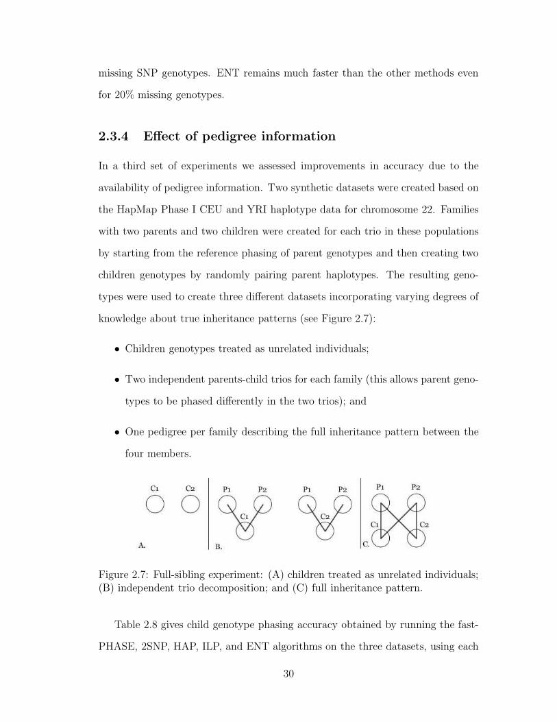
pattern. . . . . . . . . . . . . . . . . . . . . . . . . . . . . . . . . . 30
3.1 The structure of the Hidden Markov Model for n=5 SNP loci and
K=4 founders. . . . . . . . . . . . . . . . . . . . . . . . . . . . . . . 35
ix
3.2 A sample graph (a) and the corresponding HMM constructed as in
the proof of Theorem 1 (b). The groups of states associated with
each vertex are enclosed within dashed boxes. Only states reachable
from the start state are shown, with each non-start state labeled by
the allele emitted with probability 1. . . . . . . . . . . . . . . . . . 40
3.3 1-OPT tweaking procedure for improving the likelihood of a phasing. 48
4.1 Imputation-based estimates of the frequency of 0 alleles for the three
datasets vs. the real frequencies for the SNPs on Chromosome 22. 64
4.2 Accuracy and missing data rate for imputed genotypes from chro-
mosome 22 of the WTCCC study for different thresholds. The solid
line shows the discordance between imputed genotypes and original
genotype calls while the dashed line shows the missing data rate. . 65
4.3 Accuracy and missing data rate for imputed trio genotypes from
chromosome 22 of the ADHD dataset for different thresholds. The
solid line shows the discordance between imputed genotypes and
original genotype calls while the dashed line shows the missing data
rate. . . . . . . . . . . . . . . . . . . . . . . . . . . . . . . . . . . . 66
4.4 Accuracy and missing data rate for imputed genotypes from chro-
mosome 22 of the HapMap dataset for different thresholds. The
solid line shows the discordance between imputed genotypes and
original genotype calls while the dashed line shows the missing data
rate. . . . . . . . . . . . . . . . . . . . . . . . . . . . . . . . . . . . 67
5.1 The structure of the IMC model for 5 loci. . . . . . . . . . . . . . . 76
5.2 Number of bases in the global alignment of Chordata and Arthopoda
datasets. . . . . . . . . . . . . . . . . . . . . . . . . . . . . . . . . 83
x

5.3 Classification accuracy plotted versus the species size for MIN-HD
IMC and Phylo* from top to down with Arthopoda results on the
left and Chordata results on the right. . . . . . . . . . . . . . . . . 86
xi

List of Tables
2.1 Comparison between “All” and “Founders-Only” haplotype count-
ing strategies on HapMap Phase I trio populations. . . . . . . . . . 18
2.2 Properties of the HapMap Phase II dataset. . . . . . . . . . . . . . 22
2.3 Comparison results on HapMap Phase II CEU and YRI datasets. . 25
2.4 Comparison results on HapMap Phase II JPT+CHB dataset. . . . . 26
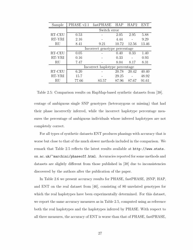
2.5 Comparison results on HapMap-based synthetic datasets from [38]. 27
2.6 Comparison results on the real dataset from [46]. . . . . . . . . . . 28
2.7 Comparison results for HapMap Phase I Chromosome 22 (15,548
SNPs for CEU and 16,386 SNPs for YRI) with 0-20% deleted SNPs. 29
2.8 Results for HapMap Phase I Chromosome 22 (15,548 SNPs for CEU
and 16,386 SNPs for YRI) full-siblings experiment. . . . . . . . . . 31
3.1 Switching error of the phasings obtained by different decoding algo-
rithms on the Orzack and ADHD X chromosome dataset. . . . . . . 50
4.1 Error Detection (ED), Error Correction (EC) Missing Data Recov-
ery (MDR) and Imputation (IMP) results obtained on the Chromo-
some 22 data for the WTCCC, ADHD and HapMap Datasets. . . . 63
5.1 Percent of barcodes with correctly recovered species by the distance-
based methods on the real datasets from [70, 40, 31, 10, 22]. . . . . . 80
xii

5.2 Percent of barcodes with correctly recovered species by the tree-
based methods on the real datasets from [70, 40, 31, 10, 22]. . . . . . 81
5.3 Percent of barcodes with correctly recovered species by the proba-
bilistic model-based methods on the real datasets from [70, 40, 31,
10, 22]. . . . . . . . . . . . . . . . . . . . . . . . . . . . . . . . . . . 81
5.4 Classification accuracy when only the Synonymous, Non-synonymous
or All the positions in the barcodes are used. . . . . . . . . . . . . . 82
5.5 Accuracy of the compared methods on datasets with different bar-
code sizes. . . . . . . . . . . . . . . . . . . . . . . . . . . . . . . . . 84
5.6 Accuracy of the compared methods on datasets with increasing
number of species. . . . . . . . . . . . . . . . . . . . . . . . . . . . 85
xiii
Chapter 1
Introduction
After the complete genome sequence for several species, including human, has
been determined, genomics research is now focusing on the study of DNA varia-
tions, with the goal of providing answers to fundamental problems ranging from
determining the genetic basis of disease susceptibility to uncovering the pattern
of historical population migrations and DNA-based species identification. These
large scale genomic studies are facilitated by recent advances in high-throughput
genomic technologies such as sequencing and SNP genotyping. Computationally,
the huge amount of data to be processed raises the need for integrating recently
developed statistical models of the structure of genomic variability with efficient
combinatorial methods delivering predictable solution quality.
A large percentage of human genomic variation is accounted by single base
mutations, in the form of single nucleotide polymorphisms (SNPs for short), i.e.,
the presence of different DNA nucleotides at certain chromosomal locations. Such
locations across the genome where different nucleotides have been observed in large
percentage of the population are also called markers and the possible nucleotides
observed at that marker are called alleles. In humans, close to 12 million common
SNPs have been cataloged in the most recent build (126) of the dbSNP database
1
maintained by NCBI (http://www.ncbi.nlm.nih.gov/projects/SNP/).
In diploid organisms such as humans, there are two non-identical copies of each
autosomal chromosome, one of maternal and the other one of paternal origin. A
description of the alleles present at SNPs along one chromosome is called a haplo-
type, while the conflated description of the SNP information on both chromosomes
is called a genotype. While the haplotype specifies the SNP alleles present on each
chromosome, the genotype specifies the identities of the two alleles at each SNP,
but does not assign the alleles to a specific chromosome.
Genotype phasing, i.e., inferring the haplotypes from genotype data, is a central
problem within the context of genomic diversity analysis as possible applications
range from missing data recovery to genotype error detection to multi-marker dis-
ease association. While there are many cost-effective high-throughput techniques
for determining the genotype data, experimental techniques for directly inferring
the haplotypes are prohibitively expensive and time consuming and thus computa-
tional methods for the genotype phasing problem have received much attention in
recent years. However, many of the existing algorithms have impractical running
time for phasing large genotype datasets such as those generated by the interna-
tional HapMap [13, 12, 11] project.
In Chapter 2 of this thesis we present a highly scalable algorithm for the geno-
type phasing problem based on the entropy minimization principle first introduced
in [42, 47, 19]. We present empirical results showing that our proposed method
achieves a phasing accuracy close to that of best existing methods while being sev-
eral orders of magnitude faster. An important feature of our proposed algorithm
is that it has the ability of using all the pedigree information available to greatly
improve the overall phasing accuracy.
Although empirical results are not conclusive, it is widely accepted that multi-
locus analysis can provide improved power to detect complex disease associations,
2
when compared with that of single-marker methods [8]. Most of the methods
for multi-locus analysis make use of the linkage observed between densely spaced
genetic markers to account for the global correlation structure in the data. In
Chapter 3 we present a hidden Markov approach toward modeling the correlation
structure between consecutive SNPs observed in a population of haplotypes [30].
Our proposed model is a left-to-right Hidden Markov Model (HMM) used to rep-
resent haplotype frequencies in the underlying population [30]. Our HMM has
a structure similar to that of models recently used for other haplotype analysis
problems including genotype phasing, testing for disease association, and imputa-
tion [32,39,51,56,58]. Intuitively, the HMM represents a small number of founder
haplotypes along high-probability “horizontal” paths of states, while capturing
observed recombinations between pairs of founder haplotypes via probabilities of
“non-horizontal” transitions. We show how this model can be used to obtain reli-
able and accurate solutions for the genotype phasing problem within a maximum
phasing probability approach. Within this context we show that it is hard to com-
pute the maximum probability phasing for a given genotype using the haplotype
frequencies represented by the HMM, answering an important problem left open
in the context of HMM-based genotype phasing. Despite the inapproximability
result we show that efficient decoding algorithms can be used to obtain accurate
solutions to the genotype phasing problem.
Since the causal SNPs are unlikely to be typed directly due to the limited
coverage of current genotyping platforms, imputation of genotypes at untyped
SNP loci has recently emerged as a powerful technique for increasing the power
of association studies [39, 56, 71, 35]. In Chapter 4 we show how our model can be
used for obtaining accurate methods for imputation of genotypes at untyped SNP
loci based on reference haplotypes such as those available in HapMap [13, 12, 11]
in conjunction with error detection and correction methods introduced in [30].
3
Imputation of missing genotypes and correction of typed genotypes is based on
conditional genotype probabilities efficiently computed using the proposed HMM.
With a runtime that scales linearly both in the number of markers and the number
of typed individuals, our algorithms are able to handle very large datasets while
achieving high accuracy rates for both imputation and error detection.
Besides whole genomic variation studies within human population, current ad-
vances in high throughput technologies, give the opportunity of analyzing the DNA
variation at a species specific level within a short region of interest in the genome.
Species specific variation of a short standardized region of the genome (called a
DNA barcode) can be used within the context of species identification and discov-
ery. Recently, DNA barcoding was proposed as a tool for differentiating biological
species [66]. The sequences currently used as barcodes are very short relative to
the entire genome and they can be obtained reasonably quickly and cheaply thus
enabling a very cost-effective species identification. Several studies show that mi-
tochondrial coding DNA can be used as a barcode because of the general accepted
assumption that mitochondrial DNA evolve at a lower rate than regular nuclear
DNA. The cytochrome c oxidase subunit 1 mitochondrial region (COI) is emerging
as the standard barcode region for almost all groups of higher animals [27]. This
region is 648 nucleotide base pairs long and is flanked by highly conserved regions,
making it relatively easy to isolate and analyze. Several studies have shown that
the inter-species variability observed within this region exceeds the intra-species
variability, thus enabling highly accurate species assignments.
Several methods for species identification have been proposed in the literature,
ranging from using simple distances between barcode sequences [52, 59] to con-
structing evolutionary trees for these short genomic regions [40]. However, to date
there is no agreed upon measure of assignment accuracy and no direct comparison
on standardized benchmarks. In Chapter 5 we attempt to fill this gap by propos-
4
ing a principled comparison methodology and performing a comprehensive study
of several of the proposed methods, including distance, tree, and statistical model
based methods. Besides the previously proposed methods we include in the com-
parison a method that relies on an extension of our HMM of haplotype diversity
from Chapter 3 to species identification. Besides assessing the accuracy and scal-
ability of individual methods on both simulated and real datasets, we also study
the effect that the number of species in the repository and number of sampled
specimens per species have on identification accuracy.
The rest of this thesis is organized as follows. We start by formally introducing
the genotype phasing problem in Chapter 2. We continue by presenting a highly
scalable algorithm based on entropy minimization principle for the genotype phas-
ing problem as well as a series of extensive experiments to assess the performance of
our algorithm. After presenting our proposed method for inferring the haplotypes
in a population, in Chapter 3 we introduce a HMM model to capture the pattern of
variation observed in the population of haplotypes. Next, we show that computing
the maximum phasing probability under this model is hard to approximate and
we introduce alternate efficiently computable likelihood functions. We continue by
introducing efficient and accurate solutions based on the HMM for other problems
arising in the context of genomic studies, such as genotype error detection and
genotype imputation in Chapter 4. While the main focus of this research has been
the study of human DNA variation, in Chapter 5 we introduce several computa-
tional approaches to the species identification problem based on DNA barcodes
and we provide a comparison with the previously proposed approaches. Finally,
we summarize the current status of this work together with possible future work
in Chapter 6.
5
Chapter 2
Genotype Phasing by Entropy
Minimization
In diploid organisms such as humans, there are two non-identical copies of each
autosomal chromosome, one inherited from the mother and one inherited from the
father. The combinations of SNP alleles in the maternal and paternal chromosomes
are referred to as the individual’s haplotypes. Although it is possible to directly
determine the multi-locus haplotypes of an individual by experimental techniques,
such methods are prohibitively expensive and time consuming. In contrast, there
are many cost-effective high-throughput techniques for determining the conflated
SNP information called genotype, which specifies the identities of the two alleles,
but does not assign the alleles to specific chromosomes. A SNP locus is called
heterozygous if different alleles are present on the chromosomes, otherwise being
referred as homozygous.
Since haplotypes determine the exact sequence (and hence function) of pro-
teins encoded by the genes, finding the haplotypes in human populations is an
important step in determining the genetic basis of complex diseases. For this
1The results presented in this chapter are based on joint work with A. Gusev and I. Mandoiu[19, 47].
6
reason, computational inference of haplotypes from genotype data, known as the
genotype phasing problem, has received much attention in the past few years, see,
e.g., [21, 23, 45, 54] for recent surveys.
In this chapter we introduce a highly scalable algorithm for genotype phasing
based on entropy minimization [42,19,47]. Experimental results on large datasets
extracted from the HapMap repository show that our method, referred to as ENT,
is several orders of magnitude faster than existing phasing methods while achieving
a phasing accuracy close to that of best existing methods. A unique feature of ENT
is that it can handle related genotypes coming from complex pedigrees, that leads
to significant improvements in phasing accuracy over methods that do not take into
account pedigree information. The open source code implementation and a web
interface are publicly available at http://dna.engr.uconn.edu/~software/ent/.
We start by introducing the terminology and formally define the genotype phas-
ing problem by entropy minimization in Section 2.1. We continue by presenting
our proposed algorithm in Section 2.2. We conclude by presenting experimental
results comparing our method to the best existing methods on well known datasets
in Section 2.3.
2.1 Problem definition
Following the standard practice we restrict our attention to bi-allelic SNPs, which
form the vast majority of known SNPs. We denote the major and minor alleles at
a SNP locus by 0 and 1. A SNP genotype represents the pair of alleles present in
an individual at a SNP locus with possible values as 0/1/2/?, where 0 and 1 denote
homozygous genotypes for the major and minor alleles, 2 denotes the heterozygous
genotype, and ? denotes missing data. At locus i SNP genotype g(i) is said to be
explained by an ordered pair of alleles (σ, σ′) ∈ {0, 1}2 if g(i) =?, or g(i) ∈ {0, 1}
7
and σ = σ′ = g(i), or g(i) = 2 and σ 6= σ′.
We denote by n the number of SNP loci typed in the population under study.
A multi-locus genotype (or simply genotype) is a 0/1/2/? vector g of length n, while
a haplotype is a 0/1 vector h of length n. We say that haplotype h is compatible
with multi-locus genotype g if g(i) = h(i) whenever g(i) ∈ {0, 1}. An ordered pair
(h, h′) of haplotypes explains multi-locus genotype g iff, for every i = 1, . . . , n, the
pair (h(i), h′(i)) explains g(i). For a given pair (h, h′) that explains G we say that
h and h′ are complementing each other with respect to G.
We call a set of genotypes unrelated if there are no parent-child relationship be-
tween the individuals from which the genotypes were obtained. We next formalize
the minimum entropy phasing problem for unrelated genotypes; phasing of related
genotypes is discussed in Section 2.2.4.
A phasing of a set of unrelated genotypes G, each of length k, is a function
φ : G → {0, 1}k × {0, 1}k, such that, for every multi-locus genotype g ∈ G, φ(g)
is a pair of haplotypes that explain g. For a haplotype h and a phasing φ, the
coverage of h under φ, denoted by cvg(h, φ), is the number of genotypes g ∈ G
such that φ(g) = (h, h′) or φ(g) = (h′, h) with h′ 6= h, plus twice the number of
genotypes g ∈ G such that φ(g) = (H, H). Notice that, for a fixed phasing, the
sum of all haplotype coverages is equal to 2|G|. As in [1,25], we define the entropy
of a phasing φ as
H(φ) =∑
h:cvg(h,φ)6=0
−cvg(h, φ)
2|G|log
cvg(h, φ)
2|G|(2.1)
The minimum entropy approach to genotype phasing was introduced by Halperin
and Karp in [25] where they also showed that a simple greedy heuristics comes close
to the optimum within additive factor of 3.
8
Definition 1 (The Minimum Entropy Phasing Problem) Given a set G of
unrelated genotypes, find a phasing φ of G with minimum entropy.
The use of entropy minimization in genotype phasing can be motivated by the fol-
lowing connection with likelihood maximization. For given haplotype probabilities
ph, the log-likelihood of a phasing φ is
L(φ) = log
(
∏
h
pcvg(h,φ)h
)
=∑
h
cvg(h, φ) log ph
= −2|G|∑
h:cvg(h,φ)6=0
−cvg(h, φ)
2|G|log ph
If ph is estimated by simply counting the number of times h appears in φ, i.e.,
ph = cvg(h,φ)2|G|
, it can be easily seen that maximizing the log-likelihood L(φ) is
equivalent with minimizing H(φ).
2.2 Proposed Algorithm
Halperin and Karp [25] proposed a greedy algorithm for the related minimum-
entropy set cover problem, and showed that a variant of this algorithm can be
applied to unrelated genotype phasing. However, the greedy algorithm cannot
be applied directly to phasing long genotypes, i.e., genotypes with large numbers
of SNPs. As the number of SNPs increases, each haplotype becomes compatible
with at most one genotype, and thus all phasings result in the same entropy of
− log 12|G|
, rendering the entropy minimization objective useless. Furthermore, even
for short genotypes, the entropy of phasings produced by the greedy algorithm
in [25] can be significantly improved as showed in [42]. Indeed, although greedy
9
phasings are guaranteed to have an entropy at most 3 bits larger than the optimum
entropy, the optimum entropy for short genotypes is typically very small. We
present here a local improvement framework approach for the entropy minimization
objective introduced in [19]. In Section 2.2.1 we describe the local improvement
algorithm for phasing short genotypes of unrelated individuals. Then, in Sections
2.2.2 and 2.2.3 we describe the extension to phasing of long unrelated genotypes and
discuss the time complexity of the algorithm. Finally, in Section 2.2.4 we describe
the extension of the local improvement algorithm to the problem of phasing long
genotypes of related individuals.
2.2.1 Short genotype phasing
We have implemented a simple local improvement algorithm for entropy minimiza-
tion. Our algorithm, which we refer to as ENT, starts from a random phasing,
then, at each step, finds the genotype whose re-explanation yields the largest de-
crease in phasing entropy (see Figure 2.1). The use of random initial phasings is
justified by observing that a random phasing of a genotype with i heterozygous
positions matches the real phasing with probability 2−i. E.g., when phasing the
children genotypes from the well-known dataset of [15], random phasing results in
an average of 46% correct haplotypes over windows of 5 consecutive SNPs. We
have also experimented with a version of the algorithm in which the initial phasing
is obtained by running the greedy algorithm of [25], which repeatedly chooses the
haplotype h that explains the maximum number of unexplained genotypes. Pre-
liminary experiments on simulated data [42] have shown that the use of random
initial phasings yields convergence to final phasings with same or slightly lower
entropy. This suggests that starting from the greedy initial solution traps the local
optimization algorithm into a poorer local optimum.
We experimented with two tie-breaking rules in step 2.1 of the algorithm: either
10
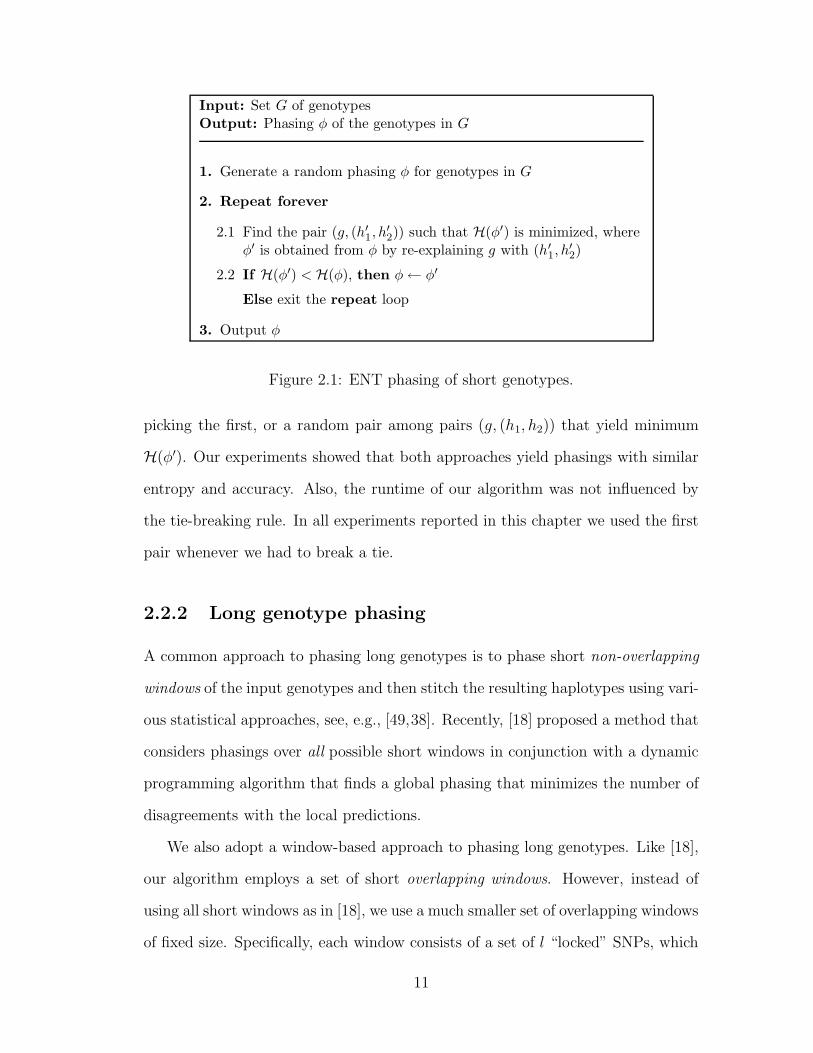
Input: Set G of genotypesOutput: Phasing φ of the genotypes in G
1. Generate a random phasing φ for genotypes in G
2. Repeat forever
2.1 Find the pair (g, (h′1, h′2)) such that H(φ′) is minimized, where
φ′ is obtained from φ by re-explaining g with (h′1, h′2)
2.2 If H(φ′) < H(φ), then φ← φ′
Else exit the repeat loop
3. Output φ
Figure 2.1: ENT phasing of short genotypes.
picking the first, or a random pair among pairs (g, (h1, h2)) that yield minimum
H(φ′). Our experiments showed that both approaches yield phasings with similar
entropy and accuracy. Also, the runtime of our algorithm was not influenced by
the tie-breaking rule. In all experiments reported in this chapter we used the first
pair whenever we had to break a tie.
2.2.2 Long genotype phasing
A common approach to phasing long genotypes is to phase short non-overlapping
windows of the input genotypes and then stitch the resulting haplotypes using vari-
ous statistical approaches, see, e.g., [49,38]. Recently, [18] proposed a method that
considers phasings over all possible short windows in conjunction with a dynamic
programming algorithm that finds a global phasing that minimizes the number of
disagreements with the local predictions.
We also adopt a window-based approach to phasing long genotypes. Like [18],
our algorithm employs a set of short overlapping windows. However, instead of
using all short windows as in [18], we use a much smaller set of overlapping windows
of fixed size. Specifically, each window consists of a set of l “locked” SNPs, which
11
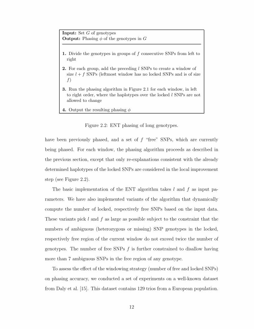
Input: Set G of genotypesOutput: Phasing φ of the genotypes in G
1. Divide the genotypes in groups of f consecutive SNPs from left toright
2. For each group, add the preceding l SNPs to create a window ofsize l + f SNPs (leftmost window has no locked SNPs and is of sizef)
3. Run the phasing algorithm in Figure 2.1 for each window, in leftto right order, where the haplotypes over the locked l SNPs are notallowed to change
4. Output the resulting phasing φ
Figure 2.2: ENT phasing of long genotypes.
have been previously phased, and a set of f “free” SNPs, which are currently
being phased. For each window, the phasing algorithm proceeds as described in
the previous section, except that only re-explanations consistent with the already
determined haplotypes of the locked SNPs are considered in the local improvement
step (see Figure 2.2).
The basic implementation of the ENT algorithm takes l and f as input pa-
rameters. We have also implemented variants of the algorithm that dynamically
compute the number of locked, respectively free SNPs based on the input data.
These variants pick l and f as large as possible subject to the constraint that the
numbers of ambiguous (heterozygous or missing) SNP genotypes in the locked,
respectively free region of the current window do not exceed twice the number of
genotypes. The number of free SNPs f is further constrained to disallow having
more than 7 ambiguous SNPs in the free region of any genotype.
To assess the effect of the windowing strategy (number of free and locked SNPs)
on phasing accuracy, we conducted a set of experiments on a well-known dataset
from Daly et al. [15]. This dataset contains 129 trios from a European population.
12
Each individual was typed at 103 SNP loci in the 5q31 region of chromosome
5. The trio genotypes were used to infer as much as possible out of the “true”
haplotypes of the children under the no-recombination assumption. We used the
genotypes of the children as input to ENT and compared the obtained phase with
the partially recovered “true” haplotypes.
0 1 2 3 4 5 6 7 8 9
1
4
7
69
1215182124273033363942454851
#locked
#free 0 1 2 3 4 5 6 7 8 9
1
4
7
69
1215182124273033363942454851
#locked
#free
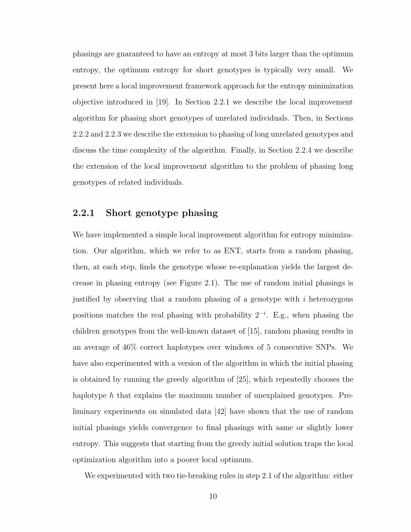
Figure 2.3: Relative switching errors obtained on the Daly children dataset by run-ning the local improvement algorithm with overlapping-windows with 0-9 lockedSNPs and 1-9 free SNPs and two optimization objectives: (left) minimizing phasingentropy, (right) minimizing the number of distinct haplotypes.
Figure 2.3(a) shows the Relative Switching Error (RSE) (see Section 2.3.1 for
the definition) obtained by running ENT with the number of locked SNPs varied
between 0 and 9, and the number of free SNPs varied between 1 and 9. As expected,
the RSE is 50% for l = 0 and f = 1, since for this setting of parameters ENT
simply produces a random phasing. As the numbers of free and locked SNPs are
increased, the entropy minimization objective quickly becomes informative, and
the RSE decreases significantly, with best results (RSE of 6.18%) being obtained
for l = f = 5 (the RSE is changing very little – within a 1% range – when setting
f and l to higher values). For this dataset, the version that dynamically chooses
13
both l and f yields minimal RSE as well. Experiments performed on other datasets
confirmed that automatically chosen f and l parameters consistently yield phasings
with RSE close to that of the best variant. Therefore, we use this variant in the
experiments presented in following sections.
To better understand the significance of using entropy minimization as opti-
mization objective for phasing short windows, we compared it with the objective
of minimizing the number of distinct haplotypes used in the phasing. This so
called pure parsimony objective was introduced in [20], which also proposes an
exponential-size integer linear program formulation. A more scalable branch-and-
bound algorithm for pure parsimony was given in [69], and polynomial-size integer
linear programs were independently proposed in [7, 34]. Figure 2.3(b) shows that,
for the considered window sizes, the RSE obtained with the pure parsimony ob-
jective is much worse than that obtained with entropy minimization.
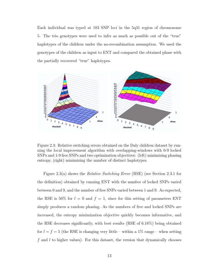
2.2.3 Time complexity
When phasing n unrelated genotypes over k SNPs, the algorithm in Figure 2.1 is
run on dk/fe windows. For each window, the algorithm evaluates at most n× 2f
candidate pairs of haplotypes for finding the best pair in Step 2.1. Computing the
entropy gain for each candidate pair takes constant time. Indeed, H(φ′) differs
from H(φ) in at most four terms corresponding to the haplotypes that can change
their coverages, namely the haplotypes explaining g in φ and φ′. Empirically, the
number of iterations required in Step 2 of the algorithm in Figure 2.1 is linear
in the number n of genotypes (see Figure 2.4), resulting in an overall runtime of
O(n22fk/f).
To reduce the number of iterations, we implemented a batched version of the
algorithm in which multiple genotypes are re-explained in each iteration. In this
version of the algorithm, an iteration starts by computing for each genotype g
14
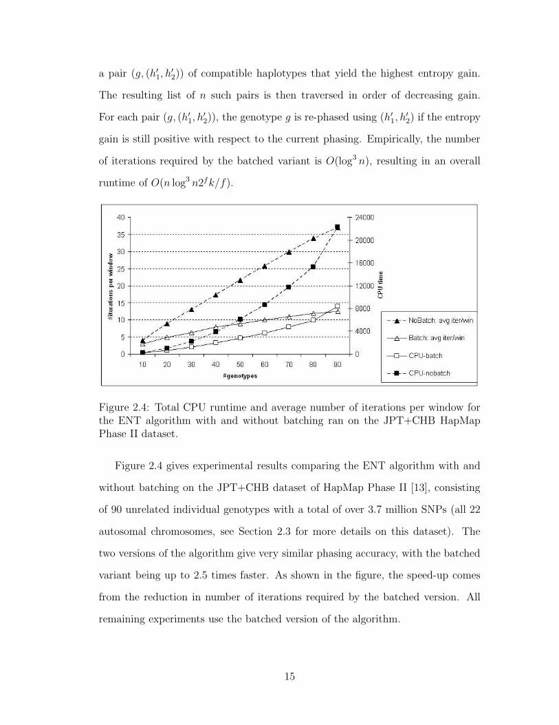
a pair (g, (h′1, h′2)) of compatible haplotypes that yield the highest entropy gain.
The resulting list of n such pairs is then traversed in order of decreasing gain.
For each pair (g, (h′1, h′2)), the genotype g is re-phased using (h′1, h
′2) if the entropy
gain is still positive with respect to the current phasing. Empirically, the number
of iterations required by the batched variant is O(log3 n), resulting in an overall
runtime of O(n log3 n2fk/f).
Figure 2.4: Total CPU runtime and average number of iterations per window forthe ENT algorithm with and without batching ran on the JPT+CHB HapMapPhase II dataset.
Figure 2.4 gives experimental results comparing the ENT algorithm with and
without batching on the JPT+CHB dataset of HapMap Phase II [13], consisting
of 90 unrelated individual genotypes with a total of over 3.7 million SNPs (all 22
autosomal chromosomes, see Section 2.3 for more details on this dataset). The
two versions of the algorithm give very similar phasing accuracy, with the batched
variant being up to 2.5 times faster. As shown in the figure, the speed-up comes
from the reduction in number of iterations required by the batched version. All
remaining experiments use the batched version of the algorithm.
15

2.2.4 Phasing related genotypes
We have also extended the ENT algorithm to handle datasets consisting of related
genotypes grouped into pedigrees. The algorithm for phasing a short window of
related genotypes is similar to the one in Figure 2.1. For every window we restrict
the search to phasings that satisfy the no-recombination assumption. To maintain
this property throughout the algorithm, in each local improvement step we re-
explain all genotypes in a pedigree rather than a single genotype.
Input: Mendelian consistent genotype data for a pedigree P together withhaplotype inheritance patternOutput: List L of feasible phasings of P
1. Let g1, . . . , g|P | be the genotypes of P indexed in reverse topological order
2. L ← ∅; i← 1; Lk ← ∅ for k = 1, . . . , |P |
3. While i > 0 do
If Li = ∅ then
If gi has descendants and their haplotypes are incompatibleunder the given inheritance pattern then
i← i− 1
Else
Set Li to the list of phasings of gi compatible withexisting descendants (if any)
ji ← 1; i← i + 1
Else // Li 6= ∅
If ji > |Li| then
Li ← ∅; i← i− 1
Else
If i = |P | then
Add to L the phasing in which each genotype gk isexplained using Lk(jk)
ji ← ji + 1
Else
ji ← ji + 1; i← i + 1
3. Output L
Figure 2.5: Bottom-up enumeration of feasible phasings for short related geno-types.
16
If entropy is computed based on haplotype counts of all typed individuals, when
re-phasing a pedigree the algorithm may introduce significant biases in haplotype
transmission rates. One way to avoid this problem is to compute the entropy
over an independent set of haplotypes, such as the “founder” haplotypes, i.e.,
haplotypes inherited from individuals not included in the pedigree. For example,
in the case of a trio, computing the entropy over all haplotypes uses six haplotypes,
while computing it over the founder haplotypes uses only the four haplotypes of the
parents. We implemented both entropy computation methods, and compared their
accuracy on CEU and YRI trio datasets from HapMap Phase I. As shown in Table
2.1, for almost all chromosomes, computing the entropy over founder haplotypes
yields slightly better accuracy. Therefore, in all remaining trio experiments we use
the founder-only entropy calculation.
An implicit representation of zero-recombination phasings for a fixed window
can be found in O(mn2 + n3 log2 n log log n) time using a system of linear equa-
tions and an efficient method for eliminating redundant equations [72]. However,
since the number zero-recombination phasings can be exponential, we chose to
generate these phasings iteratively using a backtracking strategy. Each pedigree
is represented as a directed acyclic graph with nodes representing genotypes and
directed edges connecting parents to children. Nodes that have no incoming edges
will be referred to as founder nodes. Two variants of backtracking were imple-
mented. In the top-down variant we generate the phasing for a pedigree starting
from the founder nodes and then following a topological order. This assures that,
when visiting a node, its parents are already visited. At each node, we only gen-
erate phasing compatible with the existing parent haplotypes. Once the last node
in a pedigree is phased, we compute the entropy gain and backtrack to previous
nodes to explore other feasible phasings. The bottom-up variant (Figure 2.5) it-
erates through feasible phasing in a similar manner, but starts the traversal from
17
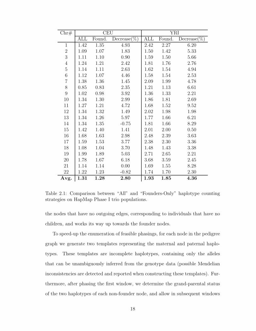
Chr# CEU YRIALL Found. Decrease(%) ALL Found. Decrease(%)
1 1.42 1.35 4.93 2.42 2.27 6.202 1.09 1.07 1.83 1.50 1.42 5.333 1.11 1.10 0.90 1.59 1.50 5.664 1.24 1.21 2.42 1.81 1.76 2.765 1.14 1.11 2.63 1.62 1.54 4.946 1.12 1.07 4.46 1.58 1.54 2.537 1.38 1.36 1.45 2.09 1.99 4.788 0.85 0.83 2.35 1.21 1.13 6.619 1.02 0.98 3.92 1.36 1.33 2.2110 1.34 1.30 2.99 1.86 1.81 2.6911 1.27 1.21 4.72 1.68 1.52 9.5212 1.34 1.32 1.49 2.02 1.98 1.9813 1.34 1.26 5.97 1.77 1.66 6.2114 1.34 1.35 -0.75 1.81 1.66 8.2915 1.42 1.40 1.41 2.01 2.00 0.5016 1.68 1.63 2.98 2.48 2.39 3.6317 1.59 1.53 3.77 2.38 2.30 3.3618 1.08 1.04 3.70 1.48 1.43 3.3819 1.99 1.89 5.03 2.71 2.65 2.2120 1.78 1.67 6.18 3.68 3.59 2.4521 1.14 1.14 0.00 1.69 1.55 8.2822 1.22 1.23 -0.82 1.74 1.70 2.30
Avg. 1.31 1.28 2.80 1.93 1.85 4.36
Table 2.1: Comparison between “All” and “Founders-Only” haplotype countingstrategies on HapMap Phase I trio populations.
the nodes that have no outgoing edges, corresponding to individuals that have no
children, and works its way up towards the founder nodes.
To speed-up the enumeration of feasible phasings, for each node in the pedigree
graph we generate two templates representing the maternal and paternal haplo-
types. These templates are incomplete haplotypes, containing only the alleles
that can be unambiguously inferred from the genotype data (possible Mendelian
inconsistencies are detected and reported when constructing these templates). Fur-
thermore, after phasing the first window, we determine the grand-parental status
of the two haplotypes of each non-founder node, and allow in subsequent windows
18
only phasings consistent with this haplotype inheritance pattern. If the algorithm
encounters a window for which a phasing consistent with this pattern cannot be
found (either due to the presence of a recombination event or poor initial choice
of haplotype inheritance pattern) we repeatedly decrease the number of free SNPs
by one unit until a feasible phasing can be found. The algorithm is then restarted
with no locked SNPs and the computed phasing is used to infer a new haplotype
inheritance pattern.
Enumerating all feasible phasings of a pedigree P for a fixed window with f free
SNPs requires O(2f |P |) time in the worst case for both backtracking variants. This
bound is achieved when all SNP genotypes are missing, and cannot be improved
since there are O(2f |P |) feasible phasings in this case. However, on typical data
the number of feasible phasings and the runtime are much lower than suggested by
the worst case bound. Despite having the same worst case runtime, the bottom-up
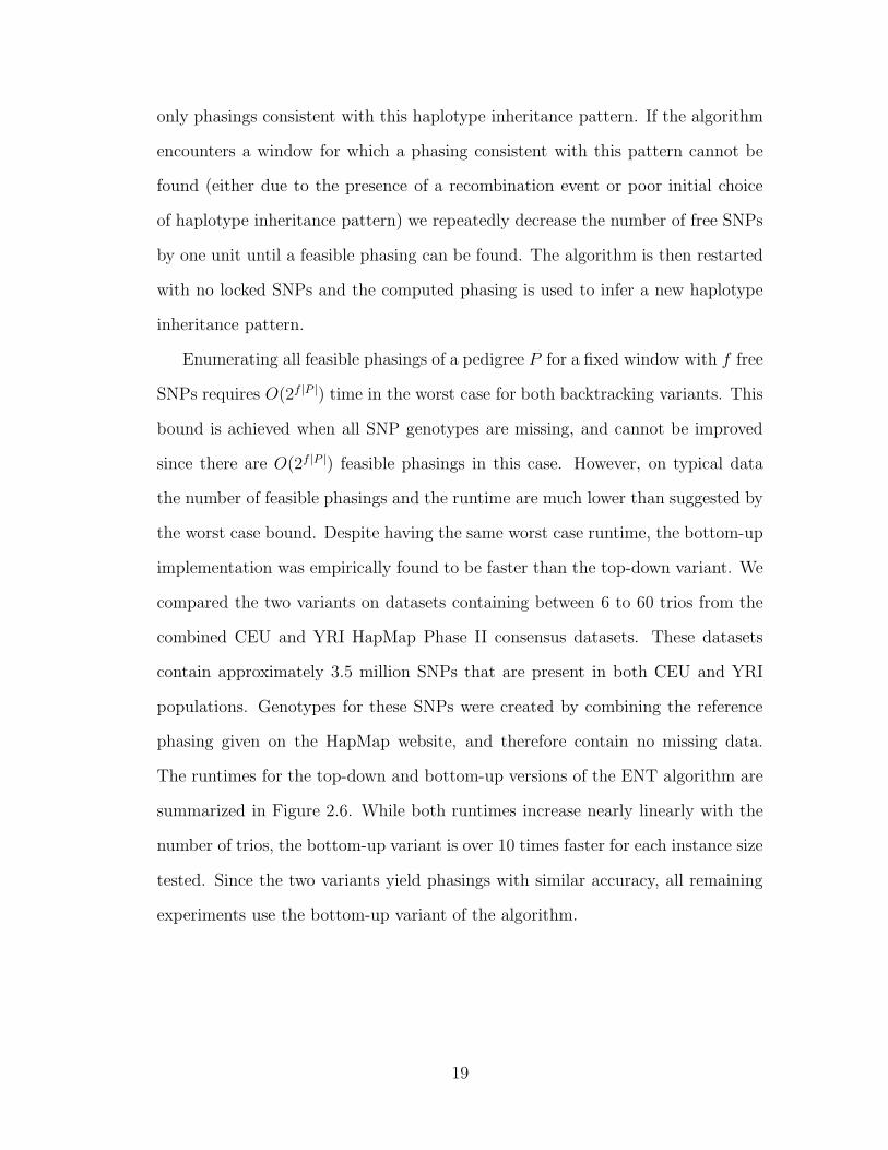
implementation was empirically found to be faster than the top-down variant. We
compared the two variants on datasets containing between 6 to 60 trios from the
combined CEU and YRI HapMap Phase II consensus datasets. These datasets
contain approximately 3.5 million SNPs that are present in both CEU and YRI
populations. Genotypes for these SNPs were created by combining the reference
phasing given on the HapMap website, and therefore contain no missing data.
The runtimes for the top-down and bottom-up versions of the ENT algorithm are
summarized in Figure 2.6. While both runtimes increase nearly linearly with the
number of trios, the bottom-up variant is over 10 times faster for each instance size
tested. Since the two variants yield phasings with similar accuracy, all remaining
experiments use the bottom-up variant of the algorithm.
19
Figure 2.6: Runtime of bottom-up and top-down ENT variants on 6-60 trios fromthe combined CEU+YRI HapMap Phase II consensus datasets.
2.3 Experimental Results
2.3.1 Experimental Setup
The ENT algorithm was implemented as described in previous section using the
C++ language. The experiments presented in this paper were conducted on a
2.8GHz Pentium Xeon machine with 4Gb of memory running the Linux operating
system.
For our experiments we used several datasets:
• HapMap Phase I datasets. HapMap [13,12,11] is a large international project
seeking to develop a haplotype map of the human genome. We used two trio
panels (CEU and YRI) consisting of 30 trio families each from the HapMap
Phase I release 16a. Since the HapMap genotypes for this release were not
consistent with the reference haplotypes, we ran the compared methods on
20
genotypes reconstructed from reference haplotypes, which resulted in geno-
types with no missing data.
• HapMap Phase II datasets. We used all three panels available in HapMap
Phase II release 21: the two trio panels (CEU and YRI) and a combined
panel consisting of the all 90 individuals from JPT and CHB populations.
For these datasets we ran the compared methods on the genotypes available
on the HapMap website. Unlike genotypes reconstructed for Phase I datasets,
these genotypes contain a small percentage of missing data. Table 2.2 shows
the number of SNPs, and the percentages of heterozygous and missing SNP
genotypes for each of the 22 autosomes in the HapMap Phase II datasets.
• HapMap-based synthetic datasets. To allow comparisons of methods that are
too slow for handling full chromosome genotype data, Marchini et al. [38]
have used the HapMap data to generate a large number of smaller simulated
datasets (referred to as “real” in [38]). RT-CEU and RT-YRI trio datasets
were obtained by selecting at random 100 1-Mb regions from each one of the
HapMap trio populations, CEU and YRI. For each region, 30 new datasets
were created by switching the allele transmission status in parent genotypes
of one of the trios (thus creating a plausible child genotype, while introducing
a minimal amount of missing data). A similar set of 100 datasets of unrelated
genotypes (RU) were generated from random 1-Mb regions from the CEU
population by simply removing children genotypes.
• Real dataset from [46]. Datasets for which the haplotypes have been directly
determined through molecular techniques such as cloning or strand-specific
PCR are the ideal testbed for comparing accuracy of haplotype inference
methods. To test if conclusions drawn from synthetic datasets remain ap-
plicable to real datasets we used the dataset from [46], consisting of 9 SNPs
21
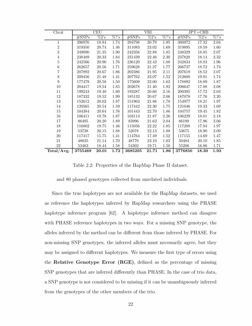
Chr# CEU YRI JPT+CHB#SNPs %2’s %?’s #SNPs %2’s %?’s #SNPs %2’s %?’s
1 296976 18.84 1.74 294798 20.79 1.95 300972 17.32 2.042 319350 20.74 1.46 311083 23.02 1.69 319895 18.59 1.603 249090 21.35 1.90 242356 22.88 1.85 248329 18.85 2.074 238489 20.33 1.84 231439 22.46 2.30 237828 18.14 2.325 242566 20.90 1.76 236120 22.43 1.88 242834 18.83 1.966 262657 20.56 1.71 259628 21.37 1.77 266737 18.72 1.737 207892 20.67 1.86 202386 21.95 2.11 207619 18.52 2.078 209456 21.48 1.41 207762 23.07 1.52 212608 19.91 1.749 177479 20.58 1.50 175609 22.00 1.62 178892 18.89 1.8710 204417 19.54 1.85 202678 21.40 1.92 206647 17.88 2.0811 199243 19.40 1.80 193287 20.60 2.16 200395 17.72 2.0312 187332 19.52 1.99 185132 20.67 2.06 187078 17.76 2.2013 152612 20.02 1.87 151963 21.86 1.78 154977 18.21 1.9714 120565 20.54 1.59 117442 22.30 1.75 121046 19.33 1.6915 104384 20.64 1.76 101443 22.70 1.86 104757 19.45 1.8216 106411 19.78 1.87 103113 21.87 2.26 106229 18.01 2.1817 86495 20.20 1.89 83996 21.62 2.04 86199 17.96 2.0618 116802 19.75 1.46 115056 22.22 1.85 117288 17.94 1.9719 53738 20.15 1.88 52078 22.13 1.88 53675 18.90 2.0920 117417 15.75 1.41 114764 17.49 1.52 117155 14.69 1.4721 48635 21.14 1.70 48770 23.10 1.62 50484 20.10 1.8522 53463 18.44 1.58 54302 19.71 1.50 55206 16.86 1.71
Total/Avg. 3755469 20.01 1.72 3685205 21.71 1.86 3776850 18.30 1.93
Table 2.2: Properties of the HapMap Phase II dataset.
and 80 phased genotypes collected from unrelated individuals.
Since the true haplotypes are not available for the HapMap datasets, we used
as reference the haplotypes inferred by HapMap researchers using the PHASE
haplotype inference program [62]. A haplotype inference method can disagree
with PHASE reference haplotypes in two ways. For a missing SNP genotype, the
alleles inferred by the method can be different from those inferred by PHASE. For
non-missing SNP genotypes, the inferred alleles must necessarily agree, but they
may be assigned to different haplotypes. We measure the first type of errors using
the Relative Genotype Error (RGE), defined as the percentage of missing
SNP genotypes that are inferred differently than PHASE. In the case of trio data,
a SNP genotype is not considered to be missing if it can be unambiguously inferred
from the genotypes of the other members of the trio.
22
A commonly used measure for the second type of error is the switching error,
which, for a given genotype, measures the ratio between the number of times we
have to switch between the inferred haplotypes to obtain the reference haplotypes.
A SNP genotype is called ambiguous if its phase cannot be fully inferred from
available data. In real data a large fraction of SNP genotypes are non-ambiguous,
e.g., homozygous SNPs, or heterozygous SNPs for which other trio members are
homozygous. Therefore, in this thesis we assess phasing accuracy using the Rel-
ative Switching Error (RSE), defined as the number of switches needed to
convert the inferred haplotype pairs into the reference haplotype pairs, expressed
as percentage of the total number of ambiguous SNPs. The positions where the
SNP genotypes are missing are ignored in the computation of RSE since errors at
these positions are separately accounted for by RGE.
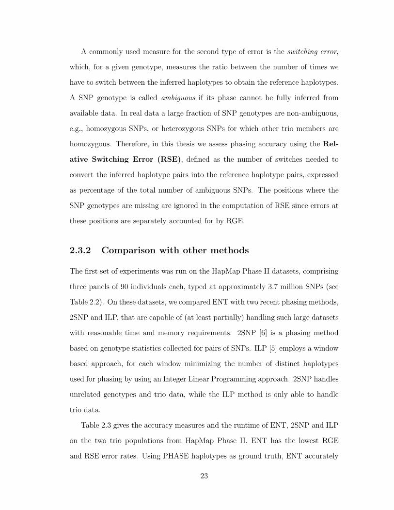
2.3.2 Comparison with other methods
The first set of experiments was run on the HapMap Phase II datasets, comprising
three panels of 90 individuals each, typed at approximately 3.7 million SNPs (see
Table 2.2). On these datasets, we compared ENT with two recent phasing methods,
2SNP and ILP, that are capable of (at least partially) handling such large datasets
with reasonable time and memory requirements. 2SNP [6] is a phasing method
based on genotype statistics collected for pairs of SNPs. ILP [5] employs a window
based approach, for each window minimizing the number of distinct haplotypes
used for phasing by using an Integer Linear Programming approach. 2SNP handles
unrelated genotypes and trio data, while the ILP method is only able to handle
trio data.
Table 2.3 gives the accuracy measures and the runtime of ENT, 2SNP and ILP
on the two trio populations from HapMap Phase II. ENT has the lowest RGE
and RSE error rates. Using PHASE haplotypes as ground truth, ENT accurately
23
recovers, on the average, more than 94% of the missing SNP genotypes for the
CEU population and more than 90% for the YRI population. On the average the
RSE of ENT is 1.51% for the CEU population and 1.94% for the YRI population,
compared to over 20% RSE for 2SNP and over 6% RSE for ILP. ENT is orders
of magnitude faster than the other two methods, requiring about half an hour for
phasing the two trio datasets, compared to over 20 hours for 2SNP and over 16
days for ILP.2
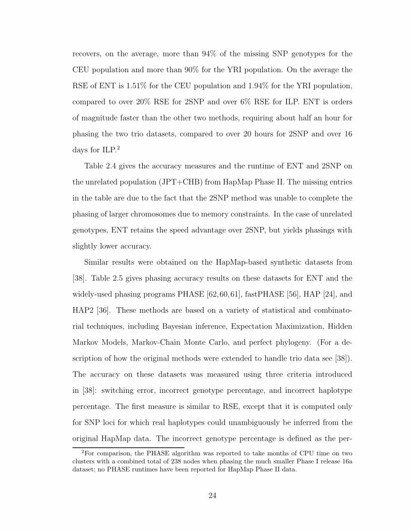
Table 2.4 gives the accuracy measures and the runtime of ENT and 2SNP on
the unrelated population (JPT+CHB) from HapMap Phase II. The missing entries
in the table are due to the fact that the 2SNP method was unable to complete the
phasing of larger chromosomes due to memory constraints. In the case of unrelated
genotypes, ENT retains the speed advantage over 2SNP, but yields phasings with
slightly lower accuracy.
Similar results were obtained on the HapMap-based synthetic datasets from
[38]. Table 2.5 gives phasing accuracy results on these datasets for ENT and the
widely-used phasing programs PHASE [62,60,61], fastPHASE [56], HAP [24], and
HAP2 [36]. These methods are based on a variety of statistical and combinato-
rial techniques, including Bayesian inference, Expectation Maximization, Hidden
Markov Models, Markov-Chain Monte Carlo, and perfect phylogeny. (For a de-
scription of how the original methods were extended to handle trio data see [38]).
The accuracy on these datasets was measured using three criteria introduced
in [38]: switching error, incorrect genotype percentage, and incorrect haplotype
percentage. The first measure is similar to RSE, except that it is computed only
for SNP loci for which real haplotypes could unambiguously be inferred from the
original HapMap data. The incorrect genotype percentage is defined as the per-
2For comparison, the PHASE algorithm was reported to take months of CPU time on twoclusters with a combined total of 238 nodes when phasing the much smaller Phase I release 16adataset; no PHASE runtimes have been reported for HapMap Phase II data.
24
CEU PopulationChr# ENT 2SNP ILP
RGE RSE Runtime RGE RSE Runtime RGE RSE Runtime1 4.82 1.63 68.12 13.24 20.76 2599 21.62 6.48 594252 5.26 1.24 83.40 13.99 17.86 3340 21.45 5.51 777023 4.68 1.41 71.72 13.94 20.72 2616 21.05 5.91 416134 4.52 1.48 59.17 13.61 20.08 3020 20.83 6.08 383475 4.73 1.36 63.10 13.83 20.23 2175 20.86 5.86 401916 4.81 1.40 66.21 13.90 20.56 2418 21.28 5.85 665597 4.82 1.52 53.70 14.15 21.12 1785 21.50 6.28 526778 4.85 1.20 50.16 13.57 17.69 1888 21.22 5.37 523939 5.04 1.35 40.22 13.14 18.25 1453 21.19 5.94 3829110 4.80 1.47 51.96 13.14 20.39 1707 21.72 6.22 5572811 4.68 1.51 48.89 13.64 20.58 1647 21.21 6.33 2832412 4.96 1.61 50.92 13.25 21.42 1568 21.79 6.51 2875813 4.83 1.47 46.65 13.54 20.85 1187 21.32 6.28 1888614 4.78 1.43 27.45 14.19 19.89 884 21.49 6.00 1285215 5.74 1.57 27.90 14.52 19.74 705 23.07 6.23 1146616 5.45 1.67 25.72 14.19 20.28 700 23.48 6.86 1266517 5.43 1.70 21.50 13.97 19.99 516 22.21 6.60 1190618 4.72 1.42 22.16 31.91 35.51 1270 20.97 6.06 1957019 5.62 1.88 12.66 14.54 21.17 356 22.54 6.78 891020 4.97 1.49 23.91 12.24 18.72 977 22.19 6.95 2965821 6.57 1.65 10.51 13.43 16.79 395 22.53 6.13 454822 5.93 1.73 12.17 12.46 17.38 314 22.94 6.97 4142
Avg./Total 5.09 1.51 938.20 14.47 20.45 33520 21.75 6.24 714611
YRI PopulationChr# ENT 2SNP ILP
RGE RSE Runtime RGE RSE Runtime RGE RSE Runtime1 8.86 2.03 89.32 18.52 23.98 2970 26.47 7.12 612772 8.75 1.67 88.34 19.82 22.80 3658 27.11 6.19 687513 8.33 1.72 72.36 19.40 23.56 3778 26.90 6.52 396904 8.71 2.05 76.35 19.02 24.61 3261 26.23 6.98 354055 8.80 1.81 68.01 19.35 23.50 3009 27.14 6.54 373086 8.06 1.73 73.51 17.98 23.18 2544 26.31 6.54 673017 8.54 1.98 63.66 19.55 24.90 1856 27.44 7.12 495808 8.78 1.55 50.34 19.27 21.10 2013 27.59 5.99 493969 8.78 1.74 48.49 19.29 21.65 1553 27.25 6.60 3681010 8.91 1.91 60.74 19.12 23.52 1963 27.33 6.99 5500411 8.38 2.03 66.54 18.71 24.74 1703 26.69 7.30 2651012 9.06 2.16 54.44 19.06 24.67 1640 28.04 7.50 2752413 8.58 1.74 41.02 18.69 22.98 1380 26.89 6.56 1826114 8.79 1.76 30.69 19.29 22.88 910 27.52 6.53 1222915 9.60 2.02 27.44 20.24 23.51 757 28.76 7.00 1086816 10.32 2.37 31.34 20.68 25.39 814 28.85 7.75 1245417 9.96 2.29 22.56 20.54 24.65 662 28.53 7.56 1122618 8.79 1.87 29.00 37.13 38.44 1420 25.86 6.61 1956819 10.48 2.47 14.26 20.15 23.02 449 28.58 7.72 853820 9.20 1.98 24.83 34.33 39.02 1069 28.68 7.70 2887121 8.73 1.75 11.30 18.45 20.89 430 26.78 6.54 458922 10.09 2.10 12.39 18.86 19.89 404 28.02 7.47 4212
Avg./Total 9.02 1.94 1056.93 20.79 24.68 38243 27.41 6.95 685372
Table 2.3: Comparison results on HapMap Phase II CEU and YRI datasets.25
JPT+CHB PopulationChr# ENT 2SNP
RGE RSE Runtime RGE RSE Runtime1 8.63 5.26 735.96 - - -2 7.84 4.48 780.27 - - -3 8.11 4.81 642.04 - - -4 8.47 4.97 619.17 - - -5 7.88 4.63 617.75 - - -6 8.59 4.75 656.95 - - -7 8.30 5.12 534.75 - - -8 9.09 4.43 571.12 - - -9 9.47 5.02 464.30 - - -10 8.66 5.17 514.10 4.93 3.13 25496011 9.77 4.92 491.08 5.50 2.82 22763012 8.79 6.00 475.08 5.51 3.79 22124513 8.04 4.94 390.07 4.69 2.90 13848114 8.39 4.77 290.93 5.18 2.98 4674115 9.83 5.33 257.82 6.07 3.57 3716616 9.58 5.89 255.55 6.23 3.99 3530017 8.98 5.97 208.62 5.64 4.16 2088618 9.27 5.22 286.31 5.37 3.23 2857619 9.97 6.75 136.46 6.82 4.96 688620 8.40 5.90 222.29 5.17 3.57 2246321 9.53 4.96 133.49 5.57 3.34 642222 10.94 6.09 128.03 6.37 3.95 6681
Avg./Total 8.93 5.24 9412.13 5.62 3.57 857495
Table 2.4: Comparison results on HapMap Phase II JPT+CHB dataset.
26
Sample PHASE v2.1 fastPHASE HAP HAP2 ENT
Switch errorRT-CEU 0.53 - 2.05 2.95 5.88RT-YRI 2.16 - 4.44 - 9.29
RU 8.41 9.21 10.72 12.56 13.46Incorrect genotype percentage
RT-CEU 0.05 - 0.40 0.33 1.40RT-YRI 0.16 - 0.33 - 0.93
RU 7.47 - 8.04 8.17 8.31Incorrect haplotype percentage
RT-CEU 6.20 - 20.78 20.42 40.40RT-YRI 15.7 - 29.25 - 48.92
RU 77.66 83.57 87.96 87.67 91.61
Table 2.5: Comparison results on HapMap-based synthetic datasets from [38].
centage of ambiguous single SNP genotypes (heterozygous or missing) that had
their phase incorrectly inferred, while the incorrect haplotype percentage mea-
sures the percentage of ambiguous individuals whose inferred haplotypes are not
completely correct.
For all types of synthetic datasets ENT produces phasings with accuracy that is
worse but close to that of the much slower methods included in the comparison. We
remark that Table 2.5 reflects the latest results available at http://www.stats.
ox.ac.uk/~marchini/phaseoff.html. Accuracies reported for some methods and
datasets are slightly different from those published in [38] due to inconsistencies
discovered by the authors after the publication of the paper.
In Table 2.6 we present accuracy results for PHASE, fastPHASE, 2SNP, HAP,
and ENT on the real dataset from [46], consisting of 80 unrelated genotypes for
which the real haplotypes have been experimentally determined. For this dataset,
we report the same accuracy measures as in Table 2.5, computed using as reference
both the real haplotypes and the haplotypes inferred by PHASE. With respect to
all three measures, the accuracy of ENT is worse than that of PHASE, fastPHASE,
27
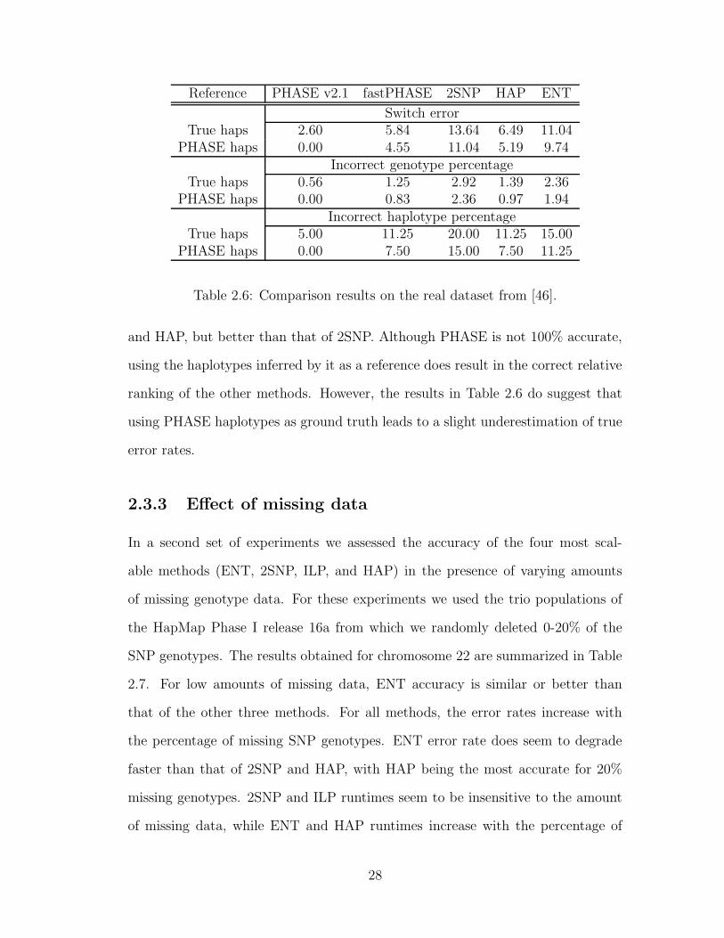
Reference PHASE v2.1 fastPHASE 2SNP HAP ENT
Switch errorTrue haps 2.60 5.84 13.64 6.49 11.04
PHASE haps 0.00 4.55 11.04 5.19 9.74Incorrect genotype percentage
True haps 0.56 1.25 2.92 1.39 2.36PHASE haps 0.00 0.83 2.36 0.97 1.94
Incorrect haplotype percentageTrue haps 5.00 11.25 20.00 11.25 15.00
PHASE haps 0.00 7.50 15.00 7.50 11.25
Table 2.6: Comparison results on the real dataset from [46].
and HAP, but better than that of 2SNP. Although PHASE is not 100% accurate,
using the haplotypes inferred by it as a reference does result in the correct relative
ranking of the other methods. However, the results in Table 2.6 do suggest that
using PHASE haplotypes as ground truth leads to a slight underestimation of true
error rates.
2.3.3 Effect of missing data
In a second set of experiments we assessed the accuracy of the four most scal-
able methods (ENT, 2SNP, ILP, and HAP) in the presence of varying amounts
of missing genotype data. For these experiments we used the trio populations of
the HapMap Phase I release 16a from which we randomly deleted 0-20% of the
SNP genotypes. The results obtained for chromosome 22 are summarized in Table
2.7. For low amounts of missing data, ENT accuracy is similar or better than
that of the other three methods. For all methods, the error rates increase with
the percentage of missing SNP genotypes. ENT error rate does seem to degrade
faster than that of 2SNP and HAP, with HAP being the most accurate for 20%
missing genotypes. 2SNP and ILP runtimes seem to be insensitive to the amount
of missing data, while ENT and HAP runtimes increase with the percentage of
28
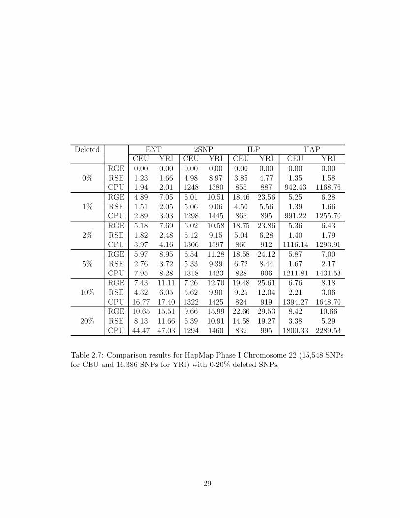
Deleted ENT 2SNP ILP HAPCEU YRI CEU YRI CEU YRI CEU YRI
RGE 0.00 0.00 0.00 0.00 0.00 0.00 0.00 0.000% RSE 1.23 1.66 4.98 8.97 3.85 4.77 1.35 1.58
CPU 1.94 2.01 1248 1380 855 887 942.43 1168.76RGE 4.89 7.05 6.01 10.51 18.46 23.56 5.25 6.28
1% RSE 1.51 2.05 5.06 9.06 4.50 5.56 1.39 1.66CPU 2.89 3.03 1298 1445 863 895 991.22 1255.70RGE 5.18 7.69 6.02 10.58 18.75 23.86 5.36 6.43
2% RSE 1.82 2.48 5.12 9.15 5.04 6.28 1.40 1.79CPU 3.97 4.16 1306 1397 860 912 1116.14 1293.91RGE 5.97 8.95 6.54 11.28 18.58 24.12 5.87 7.00
5% RSE 2.76 3.72 5.33 9.39 6.72 8.44 1.67 2.17CPU 7.95 8.28 1318 1423 828 906 1211.81 1431.53RGE 7.43 11.11 7.26 12.70 19.48 25.61 6.76 8.18
10% RSE 4.32 6.05 5.62 9.90 9.25 12.04 2.21 3.06CPU 16.77 17.40 1322 1425 824 919 1394.27 1648.70RGE 10.65 15.51 9.66 15.99 22.66 29.53 8.42 10.66
20% RSE 8.13 11.66 6.39 10.91 14.58 19.27 3.38 5.29CPU 44.47 47.03 1294 1460 832 995 1800.33 2289.53
Table 2.7: Comparison results for HapMap Phase I Chromosome 22 (15,548 SNPsfor CEU and 16,386 SNPs for YRI) with 0-20% deleted SNPs.
29
missing SNP genotypes. ENT remains much faster than the other methods even
for 20% missing genotypes.
2.3.4 Effect of pedigree information
In a third set of experiments we assessed improvements in accuracy due to the
availability of pedigree information. Two synthetic datasets were created based on
the HapMap Phase I CEU and YRI haplotype data for chromosome 22. Families
with two parents and two children were created for each trio in these populations
by starting from the reference phasing of parent genotypes and then creating two
children genotypes by randomly pairing parent haplotypes. The resulting geno-
types were used to create three different datasets incorporating varying degrees of
knowledge about true inheritance patterns (see Figure 2.7):
• Children genotypes treated as unrelated individuals;
• Two independent parents-child trios for each family (this allows parent geno-
types to be phased differently in the two trios); and
• One pedigree per family describing the full inheritance pattern between the
four members.
Figure 2.7: Full-sibling experiment: (A) children treated as unrelated individuals;(B) independent trio decomposition; and (C) full inheritance pattern.
Table 2.8 gives child genotype phasing accuracy obtained by running the fast-
PHASE, 2SNP, HAP, ILP, and ENT algorithms on the three datasets, using each
30
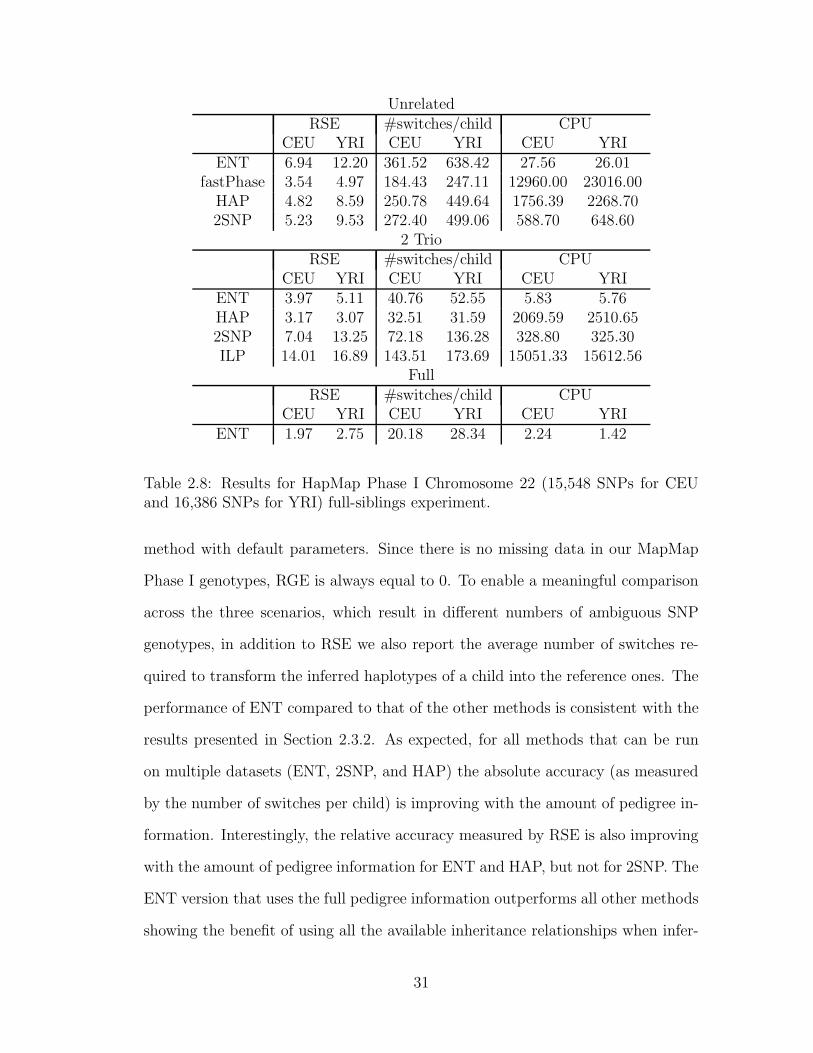
UnrelatedRSE #switches/child CPU
CEU YRI CEU YRI CEU YRIENT 6.94 12.20 361.52 638.42 27.56 26.01
fastPhase 3.54 4.97 184.43 247.11 12960.00 23016.00HAP 4.82 8.59 250.78 449.64 1756.39 2268.702SNP 5.23 9.53 272.40 499.06 588.70 648.60
2 TrioRSE #switches/child CPU
CEU YRI CEU YRI CEU YRIENT 3.97 5.11 40.76 52.55 5.83 5.76HAP 3.17 3.07 32.51 31.59 2069.59 2510.652SNP 7.04 13.25 72.18 136.28 328.80 325.30ILP 14.01 16.89 143.51 173.69 15051.33 15612.56
FullRSE #switches/child CPU
CEU YRI CEU YRI CEU YRIENT 1.97 2.75 20.18 28.34 2.24 1.42
Table 2.8: Results for HapMap Phase I Chromosome 22 (15,548 SNPs for CEUand 16,386 SNPs for YRI) full-siblings experiment.
method with default parameters. Since there is no missing data in our MapMap
Phase I genotypes, RGE is always equal to 0. To enable a meaningful comparison
across the three scenarios, which result in different numbers of ambiguous SNP
genotypes, in addition to RSE we also report the average number of switches re-
quired to transform the inferred haplotypes of a child into the reference ones. The
performance of ENT compared to that of the other methods is consistent with the
results presented in Section 2.3.2. As expected, for all methods that can be run
on multiple datasets (ENT, 2SNP, and HAP) the absolute accuracy (as measured
by the number of switches per child) is improving with the amount of pedigree in-
formation. Interestingly, the relative accuracy measured by RSE is also improving
with the amount of pedigree information for ENT and HAP, but not for 2SNP. The
ENT version that uses the full pedigree information outperforms all other methods
showing the benefit of using all the available inheritance relationships when infer-
31
ring the haplotypes. Interestingly enough, including the full pedigree information
also speeds up the ENT algorithm, as it reduces the number of zero-recombination
phasings that need to be enumerated in each local improvement iteration.
2.4 Conclusions
In this chapter we presented a highly scalable algorithm for genotype phasing based
on the entropy minimization principle. Experimental results on large datasets
extracted from the HapMap repository show that our algorithm is several orders of
magnitude faster than existing phasing methods while achieving a phasing accuracy
close to that of best existing methods. A unique feature of our algorithm is that
it can handle related genotypes coming from complex pedigrees, which can lead
to significant improvements in phasing accuracy over methods that do not take
into account pedigree information. The open source code implementation of our
algorithm and a web interface are publicly available at http://dna.engr.uconn/
edu/~software/ent/.
32
Chapter 3
A Hidden Markov Model of
Haplotype Diversity with
Applications to Genotype Phasing
In this chapter we present a left-to-right Hidden Markov Model (HMM) for repre-
senting the haplotype frequencies in the underlying population [30] by capturing
the first order Markov dependencies between pairs of consecutive loci. The struc-
ture of the model is similar to that of models recently used for other haplotype
analysis problems in this area including genotype phasing, testing for disease as-
sociation, and imputation [32, 39, 51, 56, 58]. Unlike the models in [39, 56], which
estimate a single recombination rate for every pair of consecutive SNP loci, our
model has independent transition probabilities for all pairs of states correspond-
ing to consecutive SNP loci. Intuitively, the HMM represents a small number of
founder haplotypes along high-probability horizontal paths of states, while captur-
ing observed recombinations between pairs of founder haplotypes via probabilities
of non-horizontal transitions. The biological motivation for this model comes from
1The results presented in this chapter are based, in part, on joint work with J. Kennedy andI. Mandoiu [30].
33
the assumption that, due to the presence of bottleneck events that drastically
decreased the number of distinct haplotypes in the population, the current ob-
served haplotypes must have developed from a small number of ancient founder
haplotypes by recombination and mutation events.
After describing the model we present the problem of maximum probability
genotype phasing using the HMM. Within this context we answer an important
problem left open in [51] by providing a hardness proof for the maximum proba-
bility phasing problem when haplotypes are represented by an HMM of haplotype
diversity. Following the hardness proof, we present several alternative likelihood
functions for genotype phasing proposed in the literature such as, HMM sampling,
Viterbi probability, and posterior decoding while introducing new decoding func-
tions as well as a new procedure for locally tweaking a given phasing to increase its
phasing probability. After presenting a comparison of the decoding algorithms pre-
sented throughout this chapter, we also describe a method for locally refining the
structure of the HMM by a state merging procedure within a Bayesian framework
following an approach first introduced in [63].
We start with the description of the model in Section 3.1 and continue with the
NP-hardness proof in Section 3.2. We present the likelihood functions already used
for genotype phasing in the literature, while we introduce our proposed alternate
likelihoods in Section 3.3. We conclude this chapter by presenting the Bayesian
approach to the state merging procedure for HMM structure estimation.
3.1 Hidden Markov Model of Haplotype Diver-
sity
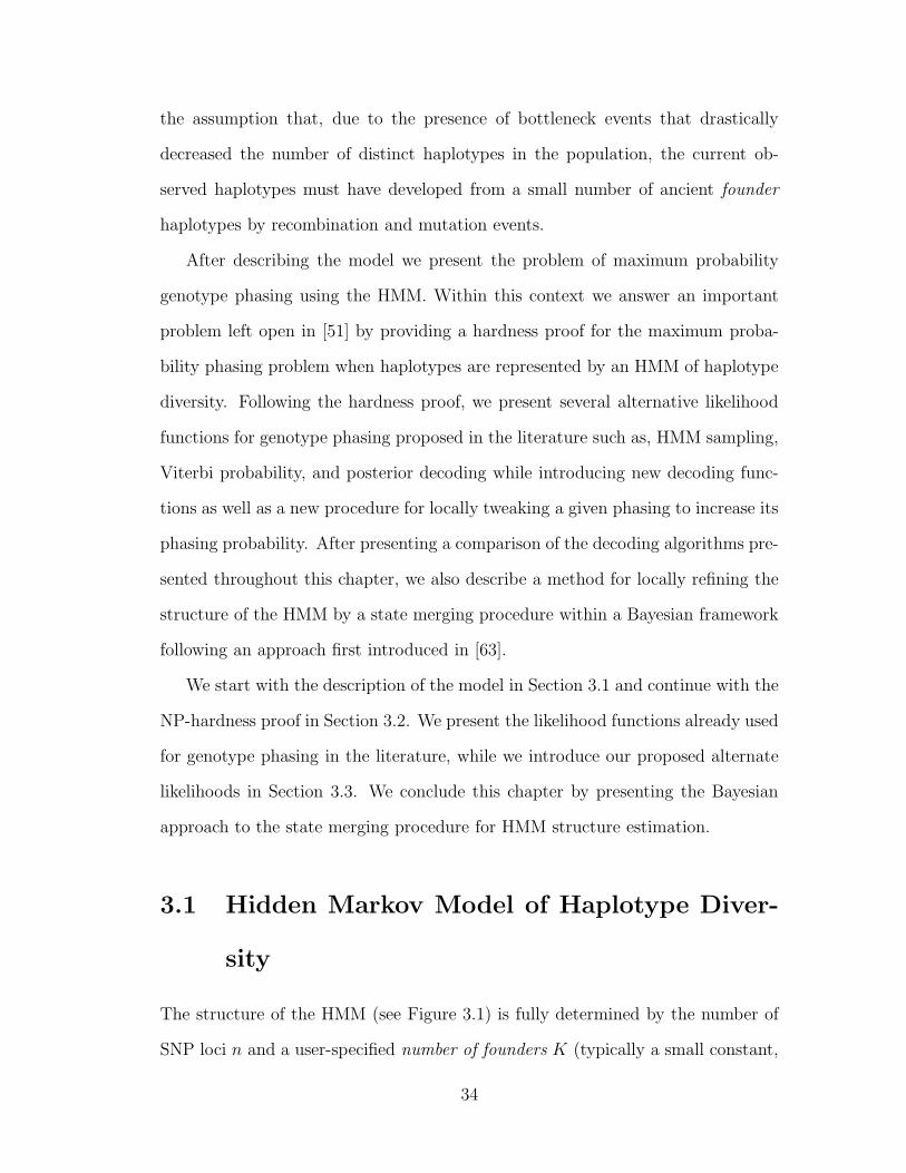
The structure of the HMM (see Figure 3.1) is fully determined by the number of
SNP loci n and a user-specified number of founders K (typically a small constant,
34
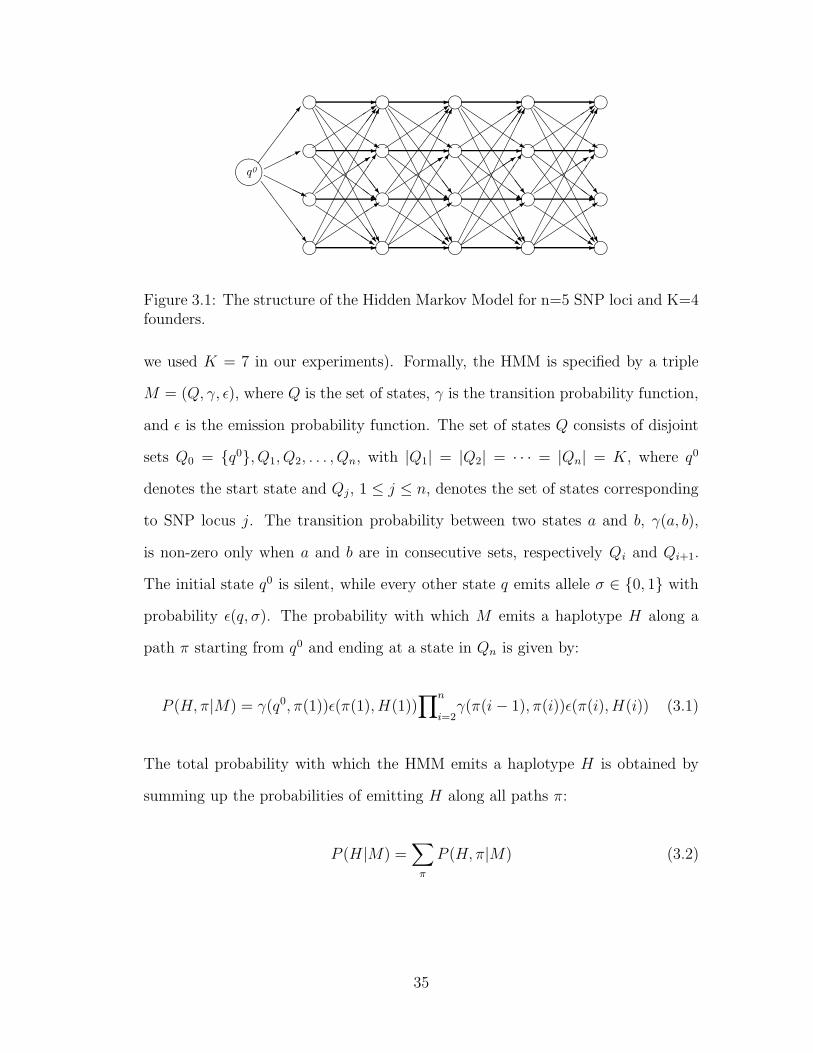
i
i
i
i
-Q
QQs
AAAAAAAAAAAU
SS
SS
SSSw
-
-
-������������
�
��
���3Q
QQs
��
���3
��
��
���7
��
���3
ZZ
ZZZ~
SS
SS
SSSw
i
i
i
i
-Q
QQs
AAAAAAAAAAAU
SS
SS
SSSw
-
-
-������������
�
��
���3Q
QQs
��
���3
��
��
���7
��
���3
ZZ
ZZZ~
SS
SS
SSSw
i
i
i
i
-Q
QQs
AAAAAAAAAAAU
SS
SS
SSSw
-
-
-������������
�
��
���3Q
QQs
��
���3
��
��
���7
��
���3
ZZ
ZZZ~
SS
SS
SSSw
i
i
i
i
-Q
QQs
AAAAAAAAAAAU
SS
SS
SSSw
-
-
-������������
�
��
���3Q
QQs
��
���3
��
��
���7
��
���3
ZZ
ZZZ~
SS
SS
SSSw
i
i
i
i
����
���*
HHHHjSS
SSSw
��
���7
q0
Figure 3.1: The structure of the Hidden Markov Model for n=5 SNP loci and K=4founders.
we used K = 7 in our experiments). Formally, the HMM is specified by a triple
M = (Q, γ, ε), where Q is the set of states, γ is the transition probability function,
and ε is the emission probability function. The set of states Q consists of disjoint
sets Q0 = {q0}, Q1, Q2, . . . , Qn, with |Q1| = |Q2| = · · · = |Qn| = K, where q0
denotes the start state and Qj, 1 ≤ j ≤ n, denotes the set of states corresponding
to SNP locus j. The transition probability between two states a and b, γ(a, b),
is non-zero only when a and b are in consecutive sets, respectively Qi and Qi+1.
The initial state q0 is silent, while every other state q emits allele σ ∈ {0, 1} with
probability ε(q, σ). The probability with which M emits a haplotype H along a
path π starting from q0 and ending at a state in Qn is given by:
P (H, π|M) = γ(q0, π(1))ε(π(1), H(1))∏n
i=2γ(π(i− 1), π(i))ε(π(i), H(i)) (3.1)
The total probability with which the HMM emits a haplotype H is obtained by
summing up the probabilities of emitting H along all paths π:
P (H|M) =∑
π
P (H, π|M) (3.2)
35
The probability P (H|M) can be computed efficiently by the forward algorithm in
time linear to the number of loci.
Given the fixed structure of our model, the next step is to estimate the tran-
sition and emission probabilities from the genotype population data in a process
known as HMM training. In [32, 51], similar HMMs were trained using genotype
data via variants of the EM algorithm. Since EM-based training is generally slow
and cannot be easily modified to take advantage of phase information that can be
inferred from available family relationships, we adopted the following two-step ap-
proach for training our HMM. First, we use the highly scalable ENT algorithm [19]
to infer haplotypes for all individuals in the sample based on entropy minimization.
As shown in Chapter 2, ENT can handle genotypes related by arbitrary pedigrees,
while yielding high phasing accuracy as measured by the switching error. The
relative small number of switches needed to transform the ENT phasing into the
true phasing, implies that the inferred haplotypes are locally correct with very high
probability. In the second step we use the classical Baum-Welch algorithm [3] to
train the HMM based on the haplotypes inferred by ENT.
3.2 Inapproximability of the Maximum Phasing
Probability Problem
In the previous section we presented a hidden Markov model that represents the
haplotype frequencies in a population under study using a first order Markovian
modeling of the dependencies between consecutive pairs of loci. We are going to
present next how to employ this model to obtain efficient and accurate solutions
for the genotype phasing problem. In [51, 58] similar models have been proposed
in the context of the genotype phasing problem with the main objective of finding
the most likely phasing for each multi-locus genotype G.
36
Regularly it is assumed that the haplotypes are drawn independently from
the population of haplotypes to form a genotype and thus the probability of a
genotype phasing φ(G) = (H1, H2) is just the product of the probabilities of the
two haplotypes given the model P (H1|M)P (H2|M). It follows that the most likely
genotype phasing problem relies on finding a pair (H1, H2) of haplotypes that
explain G with maximum P (H1|M)P (H2|M), given an HMM M (see Definition
2).
Computing P (H|M) for a given haplotype H can be easily done in O(nK)
time by using a standard forward algorithm, and thus the probability of any given
pair (H1, H2) that explains G can also be computed within the same time bound.
However, the problem of finding a pair of haplotypes with maximum phasing prob-
ability has been conjectured to be NP-hard [51] and the authors of [51, 58] settle
for efficiently computable approximations of the maximum probability genotype
phasing, ranging from using the phasing returned by the Viterbi algorithm to pick-
ing the highest probability phasing from a fixed number of phasings sampled from
the posterior distribution given by the HMM. Viterbi’s algorithm finds the pair of
haplotypes that achieve the maximum probability of being emitted along a pair
of paths (see Section 3.3.1 for details). We remark that Viterbi’s algorithm does
not necessarily yield a haplotype pair that has the highest possible probability
because the procedure relies on a single optimal pair of paths through the HMM
instead of averaging over all pairs of paths. The probability of a haplotype under
the HMM is obtained by summing the probabilities of observing that haplotype
over all possible paths.
Next, we are going to show that indeed, computing the maximum genotype
phasing probability, is hard to approximate, when haplotype frequencies are rep-
resented by a HMM of haplotype diversity.
37
Definition 2 (HMM-based Maximum Phasing Probability) Given an HMM
model M of haplotype diversity with n SNP loci and K founders and a genotype
G, compute
Pφ(G|M) = max(H1,H2),H1+H2=G
P (H1|M)P (H2|M) (3.3)
where the maximum is computed over all pairs (H1, H2) of haplotypes that explain
G.
Theorem 1 Maximum genotype phasing probability cannot be approximated within
a factor of O(n12−ε) for any ε > 0, unless ZPP=NP.
Proof. We give a reduction from the problem of computing the size of the
maximum clique in an undirected graph, refining the construction used in [37] to
show hardness of approximation for the consensus string problem.
Let G = (V, E) be a graph with n vertices V = {1, . . . , n}. We will build an
HMM MG with n + 1 SNP loci and a total of K = 4n founders. In addition
to the silent start state q0, MG contains for each vertex v of G and each SNP
locus i ∈ {0, 1, . . . , n} four states denoted qiv,j , j = 1, 2, 3, 4 such that qi
v,1 and qiv,3
emit 0 with probability 1, while qiv,2 and qi
v,4 emit 1 with probability 1. For every
v ∈ V there are two transitions from the start state q0 to q0v,2 and q0
v,3, each with
probability 2deg(v)
γ, where deg(v) denotes the degree of v in G and γ =
∑
v∈V 2deg(v)
is a normalizing constant.
Remaining non-zero probability transitions take place only from a state qi−1v,j
to a state qiv,j′ with either j, j ′ ∈ {1, 2} or j, j ′ ∈ {3, 4}. Non-zero probability
transitions within the first two “rows” of states corresponding to vertex v ∈ V
(i.e., states qiv,j with j = 1 and j = 2) are as follows:
• For every SNP locus i ∈ {1, . . . , n} \ {v} such that i is not adjacent to v in
G, MG has transitions with probability 1 from qi−1v,j , j = 1, 2, to qi
v,1
38
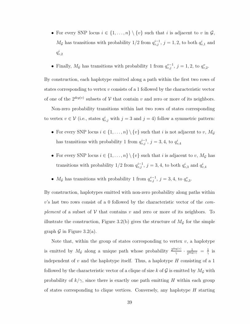
• For every SNP locus i ∈ {1, . . . , n} \ {v} such that i is adjacent to v in G,
MG has transitions with probability 1/2 from qi−1v,j , j = 1, 2, to both qi
v,1 and
qiv,2
• Finally, MG has transitions with probability 1 from qv−1v,j , j = 1, 2, to qv
v,2.
By construction, each haplotype emitted along a path within the first two rows of
states corresponding to vertex v consists of a 1 followed by the characteristic vector
of one of the 2deg(v) subsets of V that contain v and zero or more of its neighbors.
Non-zero probability transitions within last two rows of states corresponding
to vertex v ∈ V (i.e., states qiv,j with j = 3 and j = 4) follow a symmetric pattern:
• For every SNP locus i ∈ {1, . . . , n} \ {v} such that i is not adjacent to v, MG
has transitions with probability 1 from qi−1v,j , j = 3, 4, to qi
v,4
• For every SNP locus i ∈ {1, . . . , n} \ {v} such that i is adjacent to v, MG has
transitions with probability 1/2 from qi−1v,j , j = 3, 4, to both qi
v,3 and qiv,4
• MG has transitions with probability 1 from qv−1v,j , j = 3, 4, to qv
v,3.
By construction, haplotypes emitted with non-zero probability along paths within
v’s last two rows consist of a 0 followed by the characteristic vector of the com-
plement of a subset of V that contains v and zero or more of its neighbors. To
illustrate the construction, Figure 3.2(b) gives the structure of MG for the simple
graph G in Figure 3.2(a).
Note that, within the group of states corresponding to vertex v, a haplotype
is emitted by MG along a unique path whose probability 2deg(v)
γ· 1
2deg(v) = 1γ
is
independent of v and the haplotype itself. Thus, a haplotype H consisting of a 1
followed by the characteristic vector of a clique of size k of G is emitted by MG with
probability of k/γ, since there is exactly one path emitting H within each group
of states corresponding to clique vertices. Conversely, any haplotype H starting
39
� ��1
� ��3
� ��2
� ��4
@@
@@�
��
�
(a)
l1l0l0
l1-
-
���*-
-HHHj
l0l1
-
- ���*-
-HHHj
l0l1
-
- ���*-
-HHHj
l0l1
-
- ���*-
-HHHj l l l
l lll l l
l
l ll l
l
l ll l
l ll
ll
ll
ll
ll l l
l
l ll l l
l
ll
ll
l
l
l
����
HHHj- ���*
HHHj-
���*���*-
-���*
-HHHj
���*-
HHHj-
���*-
���*-
HHHj-
-HHHj
HHHj-
-
HHHj-
-
HHHj
���*
- ���*-
-���*
-HHHj
���*-
-HHHj
���*
-HHHj
-���*
-HHHj
-
-
-
0
1 1 1
0
0 0 0
1 1
0 0
1 1 1
0
1 1
0
0
1 1 1
0
0
1 1
0
0 0 0
1 1
0 0
1 1
0
1
1
0
1
0
1
0
0
Start
(b)
Figure 3.2: A sample graph (a) and the corresponding HMM constructed as inthe proof of Theorem 1 (b). The groups of states associated with each vertexare enclosed within dashed boxes. Only states reachable from the start state areshown, with each non-start state labeled by the allele emitted with probability 1.
with 1 that is emitted by MG with probability of k/γ or more defines a clique of
size k or more in G (consisting of vertices v whose groups of states emit H).
Let now G be the multi-locus genotype of length n that is heterozygous at every
SNP locus. Clearly, G can only be explained by pairs (H1, H2) of haplotypes for
which H2 = H1, where H denotes the haplotype obtained by swapping 0’s and 1’s
in H. Since the construction of MG implies that P (H|MG) = P (H|MG) for every
haplotype H, it follows that
40
Pφ(G|MG) =(
maxH
P (H|MG))2
(3.4)
and therefore G has a clique of size k or more iff P (φ(G)|MG) ≥ (k/γ)2. Since
clique is hard to approximate within a factor of O(|V|1−ε) for any ε > 0 unless
ZPP=NP [26], the theorem follows. �
Remark. Computing maximum phasing probability is closely related to the max-
imum genotype phasing problem, which, given an HMM M and a multi-locus
genotype G, asks for a pair (H1, H2) of haplotypes maximizing P (H1|M)P (H2|M).
Maximum genotype phasing was conjectured to be NP-hard by [51]. Since com-
puting phasing probability P (H1|M)P (H2|M) can be done in polynomial time for
a given pair (H1, H2) of haplotypes by two runs of the forward algorithm, Theorem
1 trivially extends to the maximum genotype phasing problem.
Similarly to computing the maximum probability genotype phasing, the prob-
lem of computing the maximum probability phasing for a mother-father-child trio
genotypes under the no recombination assumption, can be formalized as follows:
Definition 3 (HMM-based Maximum Trio Phasing Probability ) Given an
HMM model M of haplotype diversity with n SNP loci and K founders and a trio
genotype T = (Gm, Gf , Gc), find
Pφ(T |M) = max(H1,H2,H3,H4)
P (H1|M)P (H2|M)P (H3|M)P (H4|M) (3.5)
where the maximum is computed over all 4-tuples (H1, H2, H3, H4) of haplotypes
that explain T .
Theorem 2 For every ε > 0, maximum trio phasing probability cannot be approx-
imated within a factor of O(n14−ε) for any ε > 0, unless ZPP=NP.
Proof. We use a reduction similar to that in the proof of Theorem 1. When T
41
consists of three genotypes that are heterozygous at every locus, the only 4-tuples
of haplotypes that explain T are of the form (H, H, H, H) for some haplotype H.
Using the fact that P (H|MG) = P (H|MG) it follows that G has a clique of size k or
more iff P (φ(T )|MG) ≥ (k/γ)4, and the theorem follows again from the hardness
of approximation established for the clique problem in [26]. �
3.3 Efficient decoding algorithms
The hardness of approximability result from Section 3.2 motivates us into finding
alternate efficiently computable phasing likelihoods that approximate the maxi-
mum phasing probability and that lead to efficient decoding (phasing) algorithms.
3.3.1 Viterbi Decoding
A commonly used decoding method is the Viterbi algorithm, that computes the
maximum probability of emitting haplotypes that explain G along two HMM paths,
for a given multi-locus genotype (commonly known as the Viterbi probability).
After computing the Viterbi probability, a simple traceback procedure is used to
reconstruct the haplotypes that gave rise to this probability. Viterbi probability
can be computed using a trivial 2-path extension of the classical Viterbi algorithm
[68] as follows.
For every pair q = (q1, q2) ∈ Q2j , let V (j; q) denote the maximum probability of
emitting alleles that explain the first j SNP genotypes of G along a pair of paths
ending at states (q1, q2) (they are usually referred to as the Viterbi values ).
Also, let Γ(q′, q) = γ(q′1, q1)γ(q′2, q2) be the probability of transition in M from
the pair of states q′ ∈ Q2j−1 to the pair q ∈ Q2
j . Then, V (0; (q0, q0)) = 1 and
V (j; q) = E(j; q) maxq′∈Q2
j−1
{V (j − 1; q′)Γ(q′, q)} (3.6)
42
Here, E(j; q) = max(σ1 ,σ2)
∏2i=1 ε(qi, σi), where the maximum is computed over
all pairs (σ1, σ2) that explain the jth SNP genotype. For a given genotype G, the
Viterbi probability of G is given by V (T ) = maxq∈Q2n{V (n; q)}.
The time needed to compute forward Viterbi values with the above recurrences
is O(nK4), where n denotes the number of SNP loci and K denotes the number
of founders. Indeed, for each one of the O(K2) pairs q ∈ Q2j , computing the
maximum in (3.6) takes O(K2) time. However, a factor of K speed-up can be
achieved by identifying and re-using common terms between the maximums (3.6)
corresponding to different q’s [51]. Thus, instead of applying (3.6) directly we
compute, for every j, the following:
• m1(j; q1, q′2) = maxq′1∈Qj−1
{V (j− 1; (q′1, q′2))γ(q′1, q1)} for each (q1, q
′2) ∈ Qj ×
Qj−1
• V (j; q) = E(j; q) maxq′2∈Qj{m1(j; (q1, q
′2))γ(q′2, q2)} for each q = (q1, q2) ∈ Q2
j
Thus the overall time for computing the Viterbi probability for a multi-locus
genotype G is reduced to O(nK3). The genotype G is decoded (phased) as the
pair of haplotypes (H1, H2) that gave rise to the Viterbi probability (a simple
trace-back is required to obtain the pair of haplotypes).
The phasing obtained by the Viterbi algorithm does not necessarily yield a
phasing with maximum probability. Indeed, Viterbi’s algorithm computes the
maximum probability obtained by a pair of haplotypes along a single optimal pair
of paths through the HMM, instead of averaging over all pairs of paths.
3.3.2 Posterior Decoding
An alternative approach to computing the pair of haplotypes that maximizes the
phasing probability over all loci, is to choose the states that are individually most
43
likely at each locus when a pair of alleles is emitted. This approach is commonly
called posterior decoding [16]. Note that, by finding the pair of most likely states
and pair of alleles to be emitted at each locus, we are not guaranteed to find the
globally best overall haplotype pair because the total haplotype probability needs
to be summed up over all pairs of paths.
The posterior decoding picks at each locus i the pair of states (q, q ′) ∈ Q2i such
that P (i; (q, q′)|G, M) is maximized. After having the two sequences of states, the
haplotype pair that explains G emitted along the two sequences of states with the
highest phasing probability is picked as the phasing for G.
Computing P (i; (q, q′)|G, M) is done using the forward and backward algo-
rithms as follows:
P (i; (q, q′)|G, M) =pf(i; (q, q
′))× pb(i; (q, q′))
P (G|M)(3.7)
where pf(i; (q, q′)) is the total probability of emitting any two haplotypes that
explain G(1)G(2) · · ·G(i) along any pair of paths that end at (q, q ′) in level i and
is computed using the following recurrence:
pf(j; (q, q′)) = E(j; (q, q′))
∑
(s,s′)∈Q2j−1
pf(j − 1; (s, s′))Γ((s, s′), (q, q′)) (3.8)
E(j; (q, q′)) is the probability of emitting a pair of alleles at (q, q ′) ∈ Q2j that
explain G(j) and Γ((s, s′), (q, q′)) is the probability of transitioning from the pair
of states (s, s′) to pair of states (q, q′) at locus j
In a similar fashion, backward probabilities pb(i; (q, q′)) can be defined as the
probability of emitting the two haplotypes that explain G(i + 1)G(i + 2) · · ·G(n)
along any pair of paths starting at (q, q′).
Then the total probability P (G) =∑
(q,q′)∈Q2npf (n; (q, q′)) can be computed in
44
O(nK3) time using a factor k speed-up similar to the Viterbi computation.
3.3.3 Sampling Haplotype Pairs from the HMM
As proposed in [56, 51] the HMM can also be used as a generative model for
sampling pairs of haplotypes (H1, H2) from the conditional haplotype distribution
represented by the HMM, given the unphased genotype data G. This is done by
generating a sample of pairs of paths from the conditional distribution given by the
HMM and the genotype G. This can be done efficiently using a forward–backward
algorithm. In a second step from each sampled pair of paths a haplotype pair
(H1, H2) is generated from the emission probabilities conditional on the genotype
data.
While in [51] the haplotype pair that has the highest possible probability among
the pairs included in the sample is picked as the phasing for G, the authors of [56]
also experimented with a 2 loci optimization technique to construct a consensus
phasing from the sampled pairs of haplotypes in an attempt to reduce the global
switching error rate. The 2 loci optimization starts from left to right and phases
each site relative to the previous heterozygous site by selecting the two-locus haplo-
type that occurs most frequently (at that pair of sites) in the sample. The authors
of [56] also note that, since for large numbers of loci individuals may have a very
large number of compatible phasings (none of which overwhelmingly more proba-
ble than the others), the sample of phasings must be very large to reliably identify
the correct phasing by the number of appearances in the sample. Therefore the 2
loci optimization technique is preferred when the number of SNPs is large.
Unlike the authors in [56], we guide ourselves by the maximum genotype phas-
ing optimum and thus, we follow the simpler approach of [51], namely by picking
the phasing with the highest phasing probability from the sampled phasings.
45
3.3.4 Greedy Likelihood Decoding
The maximum probability phasing for a genotype G uses the pair of haplotypes
(H1, H2) that achieve the maximum P (H1|M)P (H2|M) over all pairs of haplotypes
that explain G. We introduce here an iterative left to right greedy heuristic that
chooses at each locus i the pair of alleles (H i1, H
i2) explaining G(i) such that the
probability of the phasing up to locus i is maximized, given the already determined
phasing for the first i− 1 loci (Equation 3.9).
P (H i1|M, H1
1 · · ·Hi−11 )× P (H i
2|M, H12 · · ·H
i−12 ) (3.9)
Computing the total probability of a haplotype P (H|M) can be done in time
O(Kn) using the forward algorithm, which computes for each locus i and each
state q ∈ Qi, the total probability of emitting the first i alleles of the haplotype
H and ending up at state q at level i. This values, denoted by fH(i; q) are usually
called the forward values. Then P (H|M) =∑
q∈QnfH(i; q).
In the greedy procedure, the probability in Equation 3.9 can be efficiently
computed using the forward values as follows:
∑
q∈Qi
fH1(i; q)×∑
q′∈Qi
fH2(i; q′) (3.10)
Notice that this procedure is not guaranteed to find the optimum pair of hap-
lotypes, but a reasonable pair in terms of phasing probability. The heuristic can
also be applied from right to left by following a similar approach. Moreover, a
procedure similar to the one described in Section 3.3.5 can be used to combine the
two phasings (left to right and right to left) into a phasing with possible higher
probability.
46

3.3.5 Improving the Likelihood of a Phasing by Local Switch-
ing
The posterior probabilities of the two haplotypes in the phasing, as computed by
the forward and backward algorithm can be used to compute the probability of a
new phasing obtained by performing a switch at locus l in time proportional to K
as follows. Let (H1, H2) be a phasing of G and let (H′
1, H′
2) be the phasing of G
obtained by performing a switch at position l in (H1, H2) (H′
1(i) = H1(i), 1 ≤ i < l
and H′
1(i) = H2(i), l ≤ i ≤ n).
Then P (H′
1|M)P (H′
2|M) is computed in O(K) time if the forward and back-
ward values for H1 and H2 are available, as:
∑
q∈Ql
fH1(l; q)bH2(l; q)×∑
q∈Ql
fH2(l; q)bH1(l; q)
where fH(bH) are the forward (backward) values from the forward (backward)
algorithm.
We devised a simple iterative 1-OPT tweaking procedure (see Figure 3.3) that
at each step finds the locus l that shows the highest increase in phasing probability
of the switched phasing and stops when no such improvements can be made.
A similar approach, in conjunction with Bayes’s formula is used in [64] to
devise an iterative heuristic for minimizing the total number of switching errors in
a phasing.
3.3.6 Comparison of Decoding Algorithms
In this section we provide empirical results comparing the accuracy of the decoding
algorithms presented in this chapter. In order to measure the accuracy of the
recovered phasings we use the Relative Switching Error (RSE) (see Section 2.3
47
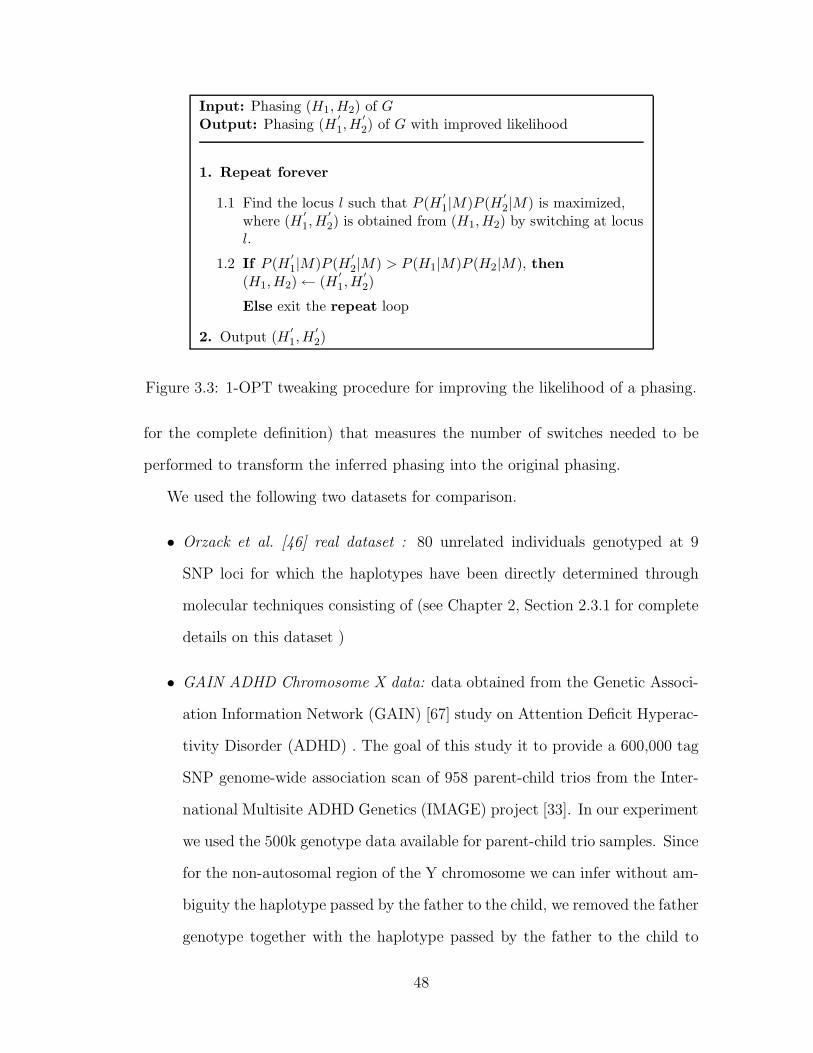
Input: Phasing (H1,H2) of G
Output: Phasing (H′
1,H′
2) of G with improved likelihood
1. Repeat forever
1.1 Find the locus l such that P (H′
1|M)P (H′
2|M) is maximized,where (H
′
1,H′
2) is obtained from (H1,H2) by switching at locusl.
1.2 If P (H′
1|M)P (H′
2|M) > P (H1|M)P (H2|M), then(H1,H2)← (H
′
1,H′
2)
Else exit the repeat loop
2. Output (H′
1,H′
2)
Figure 3.3: 1-OPT tweaking procedure for improving the likelihood of a phasing.
for the complete definition) that measures the number of switches needed to be
performed to transform the inferred phasing into the original phasing.
We used the following two datasets for comparison.
• Orzack et al. [46] real dataset : 80 unrelated individuals genotyped at 9
SNP loci for which the haplotypes have been directly determined through
molecular techniques consisting of (see Chapter 2, Section 2.3.1 for complete
details on this dataset )
• GAIN ADHD Chromosome X data: data obtained from the Genetic Associ-
ation Information Network (GAIN) [67] study on Attention Deficit Hyperac-
tivity Disorder (ADHD) . The goal of this study it to provide a 600,000 tag
SNP genome-wide association scan of 958 parent-child trios from the Inter-
national Multisite ADHD Genetics (IMAGE) project [33]. In our experiment
we used the 500k genotype data available for parent-child trio samples. Since
for the non-autosomal region of the Y chromosome we can infer without am-
biguity the haplotype passed by the father to the child, we removed the father
genotype together with the haplotype passed by the father to the child to
48
create “half-trios” (maternal genotypes with the haplotype that is passed to
the child). In this manner we preserve the existing recombination events in
the haplotype transmission from the mother to the child. In a second step,
we randomly paired half-trios to create trios with known phasing for the chil-
dren. Since some of the compared accuracy methods do not scale well with
the number of SNPs we ran all methods on the children genotypes treated
as unrelated by picking a window of 50 SNPs .
We phased the two datasets using the decoding algorithms described in this
chapter. The HMM parameters (emissions and transition probabilities) were esti-
mated using the classical Baum-Welch algorithm [3] from the haplotypes obtained
by ENT on the input genotype data. We used K=7 founders in all the experi-
ments. We compared the HMM decoding algorithms to several widely-used state
of the art phasing programs such as PHASE [62,60,61], fastPHASE [56], 2SNP [6]
and the more recent BEAGLE [9] method. PHASE employs an Expectation Max-
imization technique combined with a Markov-Chain Monte Carlo sampling from
the posterior distribution of the haplotype pairs in the population conditional on
the genotype data. The fastPHASE method uses an HMM similar to our model
but with fixed recombination rate between loci followed by haplotype pair recon-
struction from a HMM sample of phasing (see Section 3.3.3 for details). 2SNP [6]
is a phasing method based on genotype statistics collected for pairs of SNPs while
the more recent BEAGLE method employs a localized haplotype-cluster model to
construct an HMM for haplotypes followed by a phasing reconstruction step. We
show results for two variants of BEAGLE, namely when r=1 or r=4 samplings are
used in each estimation step. For a starting point in the comparison we also show
results for a trivial method that randomly assigns alleles to each haplotype in the
phasing conditioned on the genotype data (Random phasing).
Table 3.1 shows the results obtained by using the decoding algorithms on the
49
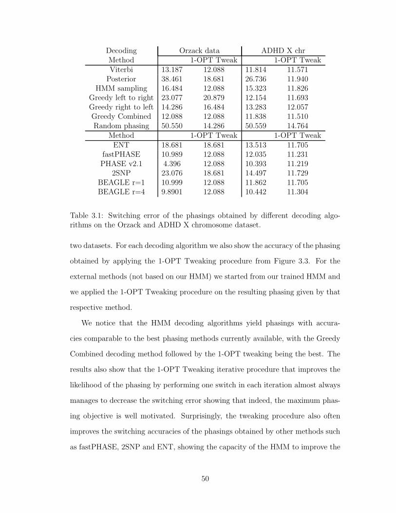
Decoding Orzack data ADHD X chrMethod 1-OPT Tweak 1-OPT TweakViterbi 13.187 12.088 11.814 11.571
Posterior 38.461 18.681 26.736 11.940HMM sampling 16.484 12.088 15.323 11.826
Greedy left to right 23.077 20.879 12.154 11.693Greedy right to left 14.286 16.484 13.283 12.057Greedy Combined 12.088 12.088 11.838 11.510Random phasing 50.550 14.286 50.559 14.764
Method 1-OPT Tweak 1-OPT TweakENT 18.681 18.681 13.513 11.705
fastPHASE 10.989 12.088 12.035 11.231PHASE v2.1 4.396 12.088 10.393 11.219
2SNP 23.076 18.681 14.497 11.729BEAGLE r=1 10.999 12.088 11.862 11.705BEAGLE r=4 9.8901 12.088 10.442 11.304
Table 3.1: Switching error of the phasings obtained by different decoding algo-rithms on the Orzack and ADHD X chromosome dataset.
two datasets. For each decoding algorithm we also show the accuracy of the phasing
obtained by applying the 1-OPT Tweaking procedure from Figure 3.3. For the
external methods (not based on our HMM) we started from our trained HMM and
we applied the 1-OPT Tweaking procedure on the resulting phasing given by that
respective method.
We notice that the HMM decoding algorithms yield phasings with accura-
cies comparable to the best phasing methods currently available, with the Greedy
Combined decoding method followed by the 1-OPT tweaking being the best. The
results also show that the 1-OPT Tweaking iterative procedure that improves the
likelihood of the phasing by performing one switch in each iteration almost always
manages to decrease the switching error showing that indeed, the maximum phas-
ing objective is well motivated. Surprisingly, the tweaking procedure also often
improves the switching accuracies of the phasings obtained by other methods such
as fastPHASE, 2SNP and ENT, showing the capacity of the HMM to improve the
50
phasing obtained by methods that trade accuracy in favor of scalability.
3.4 Refining the HMM structure
A major drawback of the HMM model of haplotype diversity presented in this
chapter is the user specified K number of founders parameter that completely
describes the global structure of the model by defining K states for each SNP.
While it is reasonable to assume that the amount of SNP variation over short
genomic regions can be described using constant number of states per SNP locus,
when trying to model the variation observed over a genome-wide area a more
suitable approach would call for a variable number of founder states per each SNP
locus.
In this section we are going to present an Bayesian approach towards estimation
the structure of our HMM of haplotype diversity, approach similar to the one
described in [63] for general HMMs. The main idea of the refinement procedure is
to start with a model that represents “best” the haplotype training dataset and
merge submodels (e.g. states) guided by the overall goal of sacrificing as little as
possible of the likelihood of the training haplotype sample H.
The starting point in our model refinement is an HMM model that is either
a) an HMM where every haplotype h in the training haplotype dataset H is
emitted along a left-to-right path with probability 1|H|
or,
b) an HMM with a very “large number” of founders in which the transition and
emission probabilities for each state are estimated using the Baum-Welch
HMM training algorithm from the training haplotype dataset H.
The merging step combines two states from the same level i, s1, s2 ∈ Qi into
a new state r where the transitions and emission probabilities of r are set as the
51
weighted averages of the probability distributions of s1 and s2. The weights are
the expected number of times s1 and s2 are observed when the haplotypes in
H are emitted. In a iterative fashion, in each iteration the pair of states s1, s2
that maximizes the Ldiff (s1, s2) = P (M ′)P (H|M ′)−P (M)P (H|M) is chosen as a
candidate merge, where M ′ is obtained from M by merging s1 and s2 and P (M),
P (M ′) are prior probabilities on the two models. The merging step is repeated as
long as Ldiff (s1, s2) is positive.
The expected number of times state s ∈ Qi is visited when generating H is
∑
h∈Hfh(i;s)bh(i;s)
P (h|M)and can be computed using the regular forward and backward
algorithms.
The probability of a haplotype in the new model with two merged states can
be computed in time O(K) by having the forward and backward values already
computed as follows.
P (h|M ′) =∑
s∈Qi\{s1,s2}
fh(i; s)bh(i; s) + fh(i; r)bh(i; r)
=∑
s∈Qi
fh(i; s)bh(i; s)− fh(i; s1)bh(i; s1)− fh(i; s2)bh(i; s2) + fh(i; r)bh(i; r)
= P (h|M)− fh(i; s1)bh(i; s1)− fh(i; s2)bh(i; s2) + fh(i; r)bh(i; r)
(3.11)
P (H|M ′) =∏
h∈H P (h|M ′) can be computed by updating each P (h|M ′) from
P (h|M) in time O(|H|K2n) since forward and backward values need to be com-
puted for each h ∈ H.
In order to compute the maximum Ldiff , n(k2) pairs of states are evaluated
giving a total runtime of O(|H|K4n2) per merge step.
52
3.4.1 Setting Priors
The simplest strategy is to use uniform priors and allow a fixed amount τ of
decrease in the posterior probability for each merging step.
The more complex option is to use priors that favor simpler models. Since the
HMM model can be described in two stages: (1) a structure (topology) specified
as a set of states, transitions and emissions (structural component Ms and (2) the
probability parameters conditional on this structure (the parameter component
θM), we can define the probability of the model P (M) as P (Ms)P (θM |Ms). An
important concern when defining priors for our model is to be able to compute
efficiently the probability of the model with two states merged (P (M ′) using the
probability of the model without merging P (M). This concern leads to using
an independence assumption between the contribution of each state to the global
prior. Then,
P (M) =∏
s
P (M sS)P (θs
M |MsS)
Dirichlet parameter priors for a state s with nst transitions and ns
e emissions:
P (θsM |M
sS) =
1
B(αt, · · · , αt)
nst∏
i=1
θαt−1si
1
B(αe, · · · , αe)
nse∏
i=1
θαe−1si
where θ’s are transition/emissions probabilities and α’s are the prior weights bi-
asing more or less towards uniform assignment of the parameters. Specifically for
our model ne = 2 for all states and nt ≤ K.
The structural component of the prior deals only with the number of states
since all the other components of the model are incorporated in the parameters
priors. In this case P (M)αC |−Q|. A particular case is the Minimum Description
53
Length prior: P (M)αe−l(M). The resulting prior
P (M sS)α(|Q|+ 1)−ns
t (|Σ|+ 1)nse
gives more weight to changes in number of transitions and emissions rather than
number of states.
3.5 Conclusions
In this chapter we have presented a Hidden Markov Model that represents the
haplotype diversity in a population. The proposed HMM has a structure similar
to that of models recently used for other haplotype analysis problems including
genotype phasing, testing for disease association, and imputation [32,39,51,56,58].
We started by showing that computing the maximum phasing probability, in the
case of unrelated as well as trio data is hard to approximate, solving an important
problem left open in the context of HMM phasing in [51]. After showing that
computing the maximum probability phasing is NP-hard we focused on alternate
efficiently computable likelihood functions previously used in this context. We
introduced a new likelihood function that picks the allele pair at each locus in a
greedy fashion conditional on the previously picked alleles in a left to right or right
to left order as well as a method for combining them. We also introduced a 1-
OPT tweaking procedure for improving the likelihood of the phasing that at each
step finds the switch that gives the best improve in the likelihood and updates
the phasing. We showed that on real genotype datasets our proposed decoding
algorithms are comparable in terms of switching accuracy to the best existing
phasing methods.
54
Chapter 4
HMM-based Genotype
Imputation
Genome-wide case-control association studies are currently the preferred method
for uncovering the genetic basis of complex human diseases. These studies follow
a simple methodology of typing a very large number of markers, in individuals
affected by the disease, cases, and in individuals not showing the disease, controls,
followed by a statistical test of association to find the markers that show the high-
est correlation with the disease status. The validity of associations uncovered in
genome-wide association studies critically depends on the accuracy of the geno-
type data. Despite recent progress in genotype calling algorithms, significant error
levels remain present in SNP genotype data, see [48] for a recent survey. Current
association studies assay a very large set of SNPs across the whole genome, e.g
the 500k Affymetrix chip [65], in the attempt of finding the region most correlated
with the disease status. Due to the vast number of markers present across the
human genome it is usually assumed that the true causal SNP will not be typed
directly due to the limited coverage of current genotyping platforms. Using the
1The results presented in this chapter are part of ongoing joint work with J. Kennedy and I.Mandoiu.
55
typed markers as “predictors” for the true causal SNP not present on the array has
recently emerged as a powerful technique for increasing the power of association
studies [39, 56, 71, 35]. Finding and explaining association signals relies on remov-
ing the genotype errors as well as on the ability of performing statistical analyses
at untyped loci. The additional required information for imputing missing SNPs
comes from large repositories of variations such as the HapMap project [13,12,11].
The three panels of the HapMap projects, composed of individuals typed at vast
number SNPs, can be used in conjunction with the genotypes typed in the associ-
ation study to predict genotypes at markers (e.g. SNPs) not present on the assay
used in the study. The major challenge of this approach relies in optimally combin-
ing the multi-locus information observed in the current study with the multi-locus
variation already cataloged in variation repositories, such as HapMap.
In this chapter we present the extension of the HMM model described in Chap-
ter 3 to imputing genotypes at untyped SNP loci by combining the information
from the genotypes typed in the current association study with the reference hap-
lotype data from the panels of HapMap [13, 12, 11] as a first step in subsequent
analyses. Imputation of missing genotypes is based on multi-locus genotype like-
lihoods efficiently computed using the HMM of haplotype diversity that captures
the Linkage Disequilibrium (LD) observed in the population under study.
With a runtime that scales linearly both in the number of markers and the
number of typed individuals, our methods are able to handle very large datasets
while achieving high accuracy rates for genotype imputation.
4.1 Imputation Likelihood
The HMM described in Chapter 3 provides a very compact representation of the
haplotype frequencies in the populations, representation that can be employed to
56
obtain efficient methods for imputing genotypes at untyped SNPs.
In a first step we integrate the HapMap variation information by using the
haplotypes from the panel related to the population in the current study (e.g.
CEU panel composed of Utah residents with ancestry from northern and western
Europe) to estimate the transition and emissions probabilities of the HMM. In the
second step, imputation of genotypes at untyped loci is performed using conditional
probabilities from the HMM model as follows.
The probability of imputing missing genotype gi as x in G at locus i can be
written in terms of our HMM as follows:
P (gi = x|G, M) =P (G, gi = x|M)
P (G|M)=
P (Ggi←x|M)
P (G|M)(4.1)
where Ggi←x denotes the multi-locus genotype obtained from G by replacing
the i-th SNP genotype with x, where x ∈ {0, 1, 2}. Imputation is then done by
setting the untyped gi as
x∗ = argmaxx∈{0,1,2}
P (Ggi←x|M)
P (G|M)(4.2)
Notice that the same approach can be used to infer missing genotype calls in the
context of the Missing Data Recovery problem that seeks to fill in the genotypes
uncalled by the genotype calling algorithm with the most probable ones.
When gi is called as genotype a, P (G|M) = P (Ggi←a|M) can be used to detect
potential genotype calling errors in a likelihood ratio framework as
P (Ggi←?|M)
P (G|M)=
∑
x∈{0,1,2} P (Ggi←x|M)
P (Ggi←a|M)(4.3)
measures the likelihood increase obtained by setting that respective genotype
to missing. If the increase is higher than a given threshold then gi is flagged
57
as a potential error. Methods for genotype error detection that use the HMM
to compute the likelihood ratio from Equation 4.3 have been introduced in [30].
These methods extend the likelihood ratio error detection approach of Becker et
al. [4]. Unlike Becker et al., that adopt a window-based approach and rely on
creating a short list of frequent haplotypes within each window, using the HMM
(see Chapter 3) for likelihood computations has the main advantage of representing
frequencies of all haplotypes over the set of typed loci. For comprehensive results
on error detection using the likelihood ratio approach in the context of the HMM,
the reader is directed to [30].
We introduce here a similar approach that can be used not only to detect
but also to correct possible genotype calling errors by replacing gi = a with new
genotype x when the following ratio
maxx∈{0,1,2}P (Ggi←x|M)
P (G|M)=
P (Ggi←x|M)
P (Ggi←a|M)(4.4)
that measures the gain in likelihood when genotype gi is is re-called as x, exceeds
a user specified threshold.
We have implemented extensions of the above imputation methods to the case
when the input consists of genotype data from related individuals coming from
mother-father-child nuclear families (trios). In this case the imputation is still
done one SNP genotype at a time, but imputation probabilities are computed over
genotype data of the entire trio nuclear family.
The forward algorithm in regular HMMs computes the probability of emitting
a sequence of emissions along all possible paths of states. We present next the
extensions of the forward algorithm to pairs of paths for computing the total
probabilities of emitting a pair of haplotypes along any pair of paths that explain
a given genotype. We also present an efficient computation for computing the
58
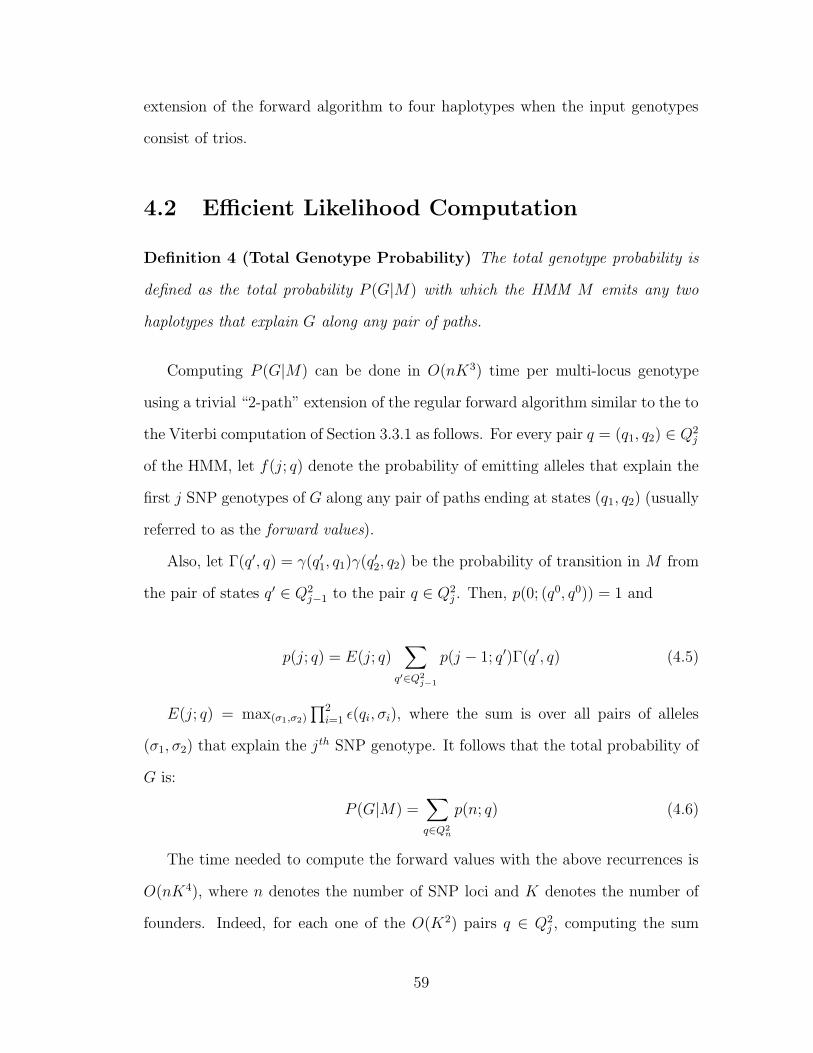
extension of the forward algorithm to four haplotypes when the input genotypes
consist of trios.
4.2 Efficient Likelihood Computation
Definition 4 (Total Genotype Probability) The total genotype probability is
defined as the total probability P (G|M) with which the HMM M emits any two
haplotypes that explain G along any pair of paths.
Computing P (G|M) can be done in O(nK3) time per multi-locus genotype
using a trivial “2-path” extension of the regular forward algorithm similar to the to
the Viterbi computation of Section 3.3.1 as follows. For every pair q = (q1, q2) ∈ Q2j
of the HMM, let f(j; q) denote the probability of emitting alleles that explain the
first j SNP genotypes of G along any pair of paths ending at states (q1, q2) (usually
referred to as the forward values).
Also, let Γ(q′, q) = γ(q′1, q1)γ(q′2, q2) be the probability of transition in M from
the pair of states q′ ∈ Q2j−1 to the pair q ∈ Q2
j . Then, p(0; (q0, q0)) = 1 and
p(j; q) = E(j; q)∑
q′∈Q2j−1
p(j − 1; q′)Γ(q′, q) (4.5)
E(j; q) = max(σ1,σ2)
∏2i=1 ε(qi, σi), where the sum is over all pairs of alleles
(σ1, σ2) that explain the jth SNP genotype. It follows that the total probability of
G is:
P (G|M) =∑
q∈Q2n
p(n; q) (4.6)
The time needed to compute the forward values with the above recurrences is
O(nK4), where n denotes the number of SNP loci and K denotes the number of
founders. Indeed, for each one of the O(K2) pairs q ∈ Q2j , computing the sum
59
in (3.6) takes O(K2) time. However, a factor of K speed-up cane be achieved,
similarly to the Viterbi computation of Section 3.3.1 by identifying and re-using
common terms between the sums (4.5) corresponding to different q’s [51].
Thus the overall time for computing the probability for a multi-locus genotype
G is reduced to O(nK3).
Definition 5 (Total Trio Genotype Probability) The total trio genotype prob-
ability is defined as the total probability P (T |M) with which the HMM M emits
any four haplotypes that explain T along any 4-tuple of paths.
Using again an extension of the forward algorithm, P (T ) can be computed as∑
q∈Q4n
p(n; q), where p(0; (q0, q0, q0, q0)) = 1 and
p(j; q) = E(j; q)∑
q′∈Q4j−1
p(j − 1; q′)Γ(q′, q) (4.7)
The time needed to compute P (T ) with the standard recurrence is O(nK8), but a
K3 speed-up can again be achieved by re-using common terms and computing, in
order:
• s1(j; q1, q′2, q′3, q′4) =
∑
q′1∈Qj−1p(j−1; (q′1, q
′2, q′3, q′4))γ(q′1, q1) for each (q1, q
′2, q′3, q′4) ∈
Qj ×Q3j−1
• s2(j; q1, q2, q′3, q′4) =
∑
q′2∈Qj−1s1(j; (q1, q
′2, q′3, q′4))γ(q′2, q2) for each (q1, q2, q
′3, q′4) ∈
Q2j ×Q2
j−1
• s3(j; q1, q2, q3, q′4) =
∑
q′3∈Qj−1s2(j; (q1, q2, q
′3, q′4))γ(q′3, q3) for each (q1, q2, q3, q
′4) ∈
Q3j ×Qj−1
• p(j; q) = E(j; q)∑
q′4∈Qj−1s3(j; (q1, q2, q3, q
′4))γ(q′4, q4) for each q = (q1, q2, q3, q4) ∈
Q4j
This allows computing P (T |M) in O(nK5) time.
60
4.3 Experimental Results
We introduce here a combined approach for the genotype imputation problem, in
which imputation is performed in conjunction with error correction and missing
data recovery. We extended the HMM-based methods for error detection proposed
in [30] to error correction and missing data recovery as described in Section 4.1.
We distinguish among three possible flows for genotype imputation:
• IMP: genotypes at un-typed SNP were imputed using the original genotype
data
• MDR+IMP: first, the missing genotypes at typed SNPs were recovered,
then the complete data was used for imputation of un-typed SNP genotypes
• EDC+MDR+IMP: first, erroneous genotypes were detected and corrected,
second, the corrected genotypes were used to recover missing genotypes at
typed SNPs, then the complete data was used to impute genotypes at un-
typed SNPs
We used the HapMap CEU haplotypes (obtained using the well-known PHASE
software) as a reference panel for imputation of genotypes at un-typed SNPs. Since
in the error detection and missing data recovery steps, the HMM is trained such
that it captures “best” the haplotype frequencies of the population under study,
we experimented with two approaches. In the first approach, we trained the HMM
using the haplotypes inferred by ENT from the genotypes in the study (see Chapter
2 for details on ENT). In the second approach we used the reference reference CEU
haplotypes obtained by PHASE for estimating the parameters of our HMM.
The following datasets were used in our experiments:
• WTCCC Dataset: genotype data of the 1958 birth cohort of the Wellcome
Trust Case Control Consortium (WTCCC) study [14] containing 1,444 indi-
61
viduals typed using the Affymetrix 500k platform. We inserted 1% errors in
genotype calls, set 1% of the genotype calls as missing and masked 1% of the
SNPs as un-typed
• ADHD Dataset: genotype data from the Genetic Association Informa-
tion Network (GAIN) [67] study on attention deficit hyperactivity disorder
(ADHD) . The goal of this study it to provide a 600,000 tag SNP genome-
wide association scan of 958 parent-child trios from the International Mul-
tisite ADHD Genetics (IMAGE) project [33]. In our experiment we used
the Perlgen500k genotype data available for the 958 mother-father-child trio
samples. We inserted 1% errors in genotype calls, set 1% of the genotype
calls as missing and masked 1% of the SNPs as un-typed
• HapMap Dataset: the HapMap CEU panel consisting of 30 mother-father-
child trio families residents of Utah with European ancestry were genotyped
using both the Affymetrix 500k platform and the Affymetrix 6.0 platforms.
Affymetrix 500k genotypes were used to impute genotypes left un-called
and genotypes of SNPs on the Affymetrix 6.0 platform not covered by the
Affymetrix 500k. Actual Affymetrix 6.0 genotypes were assumed to be cor-
rect when estimating imputation and missing data recovery accuracy. In par-
ticular disagreements between Affymetrix 500k and 6.0 calls were assumed
to be correct in 6.0 data
We assessed the accuracy of our methods for each step using well known mea-
sures. Error Detection True Positive (TP) Rate measures the percentage of the
genotype errors inserted that get correctly flagged. The Error Detection False
Positive (FP) Rate is the percentage of correct genotype calls that get erroneously
flagged. Notice that we overestimate the FP rate by assuming that all the geno-
type calls in the genotypes from the three datasets are correct. Error Correction
62
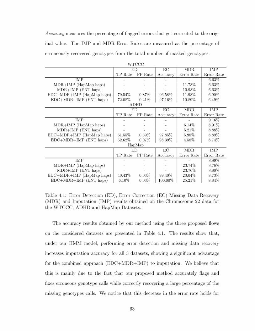
Accuracy measures the percentage of flagged errors that get corrected to the orig-
inal value. The IMP and MDR Error Rates are measured as the percentage of
erroneously recovered genotypes from the total number of masked genotypes.
WTCCCED EC MDR IMP
TP Rate FP Rate Accuracy Error Rate Error RateIMP - - - - 6.63%
MDR+IMP (HapMap haps) - - - 11.78% 6.63%MDR+IMP (ENT haps) - - - 10.98% 6.63%
EDC+MDR+IMP (HapMap haps) 79.54% 0.87% 96.58% 11.98% 6.90%EDC+MDR+IMP (ENT haps) 72.08% 0.21% 97.16% 10.89% 6.49%
ADHDED EC MDR IMP
TP Rate FP Rate Accuracy Error Rate Error RateIMP - - - - 9.16%
MDR+IMP (HapMap haps) - - - 6.14% 8.91%MDR+IMP (ENT haps) - - - 5.21% 8.88%
EDC+MDR+IMP (HapMap haps) 61.55% 0.39% 97.85% 5.98% 8.89%EDC+MDR+IMP (ENT haps) 52.62% 0.07% 98.39% 4.58% 8.74%
HapMapED EC MDR IMP
TP Rate FP Rate Accuracy Error Rate Error RateIMP - - - - 8.89%
MDR+IMP (HapMap haps) - - - 23.74% 8.76%MDR+IMP (ENT haps) - - - 23.76% 8.80%
EDC+MDR+IMP (HapMap haps) 40.43% 0.03% 99.40% 23.04% 8.73%EDC+MDR+IMP (ENT haps) 6.10% 0.03% 100.00% 25.21% 8.84%
Table 4.1: Error Detection (ED), Error Correction (EC) Missing Data Recovery(MDR) and Imputation (IMP) results obtained on the Chromosome 22 data forthe WTCCC, ADHD and HapMap Datasets.
The accuracy results obtained by our method using the three proposed flows
on the considered datasets are presented in Table 4.1. The results show that,
under our HMM model, performing error detection and missing data recovery
increases imputation accuracy for all 3 datasets, showing a significant advantage
for the combined approach (EDC+MDR+IMP) to imputation. We believe that
this is mainly due to the fact that our proposed method accurately flags and
fixes erroneous genotype calls while correctly recovering a large percentage of the
missing genotypes calls. We notice that this decrease in the error rate holds for
63
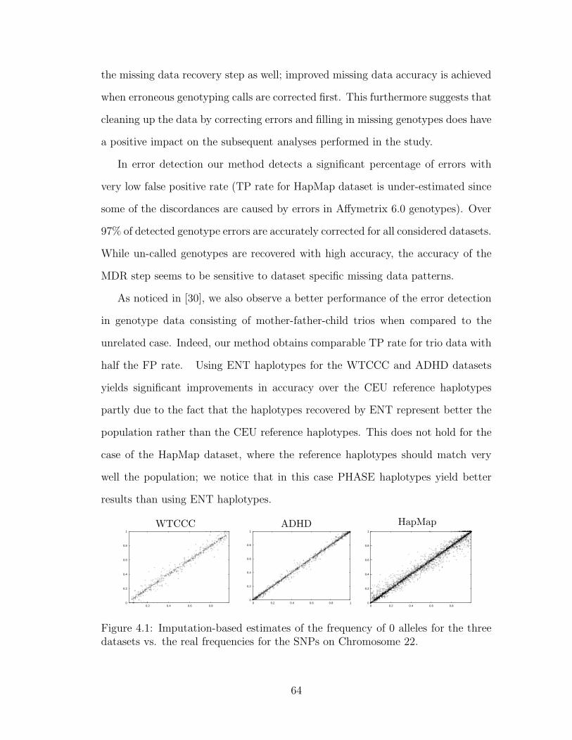
the missing data recovery step as well; improved missing data accuracy is achieved
when erroneous genotyping calls are corrected first. This furthermore suggests that
cleaning up the data by correcting errors and filling in missing genotypes does have
a positive impact on the subsequent analyses performed in the study.
In error detection our method detects a significant percentage of errors with
very low false positive rate (TP rate for HapMap dataset is under-estimated since
some of the discordances are caused by errors in Affymetrix 6.0 genotypes). Over
97% of detected genotype errors are accurately corrected for all considered datasets.
While un-called genotypes are recovered with high accuracy, the accuracy of the
MDR step seems to be sensitive to dataset specific missing data patterns.
As noticed in [30], we also observe a better performance of the error detection
in genotype data consisting of mother-father-child trios when compared to the
unrelated case. Indeed, our method obtains comparable TP rate for trio data with
half the FP rate. Using ENT haplotypes for the WTCCC and ADHD datasets
yields significant improvements in accuracy over the CEU reference haplotypes
partly due to the fact that the haplotypes recovered by ENT represent better the
population rather than the CEU reference haplotypes. This does not hold for the
case of the HapMap dataset, where the reference haplotypes should match very
well the population; we notice that in this case PHASE haplotypes yield better
results than using ENT haplotypes.
WTCCC
0
0.2
0.4
0.6
0.8
1
0.80.60.40.2
ADHD
0
0.2
0.4
0.6
0.8
1
0 0.2 0.4 0.6 0.8 1
x
HapMap
0
0.2
0.4
0.6
0.8
1
0.80.60.40.20
Figure 4.1: Imputation-based estimates of the frequency of 0 alleles for the threedatasets vs. the real frequencies for the SNPs on Chromosome 22.
64
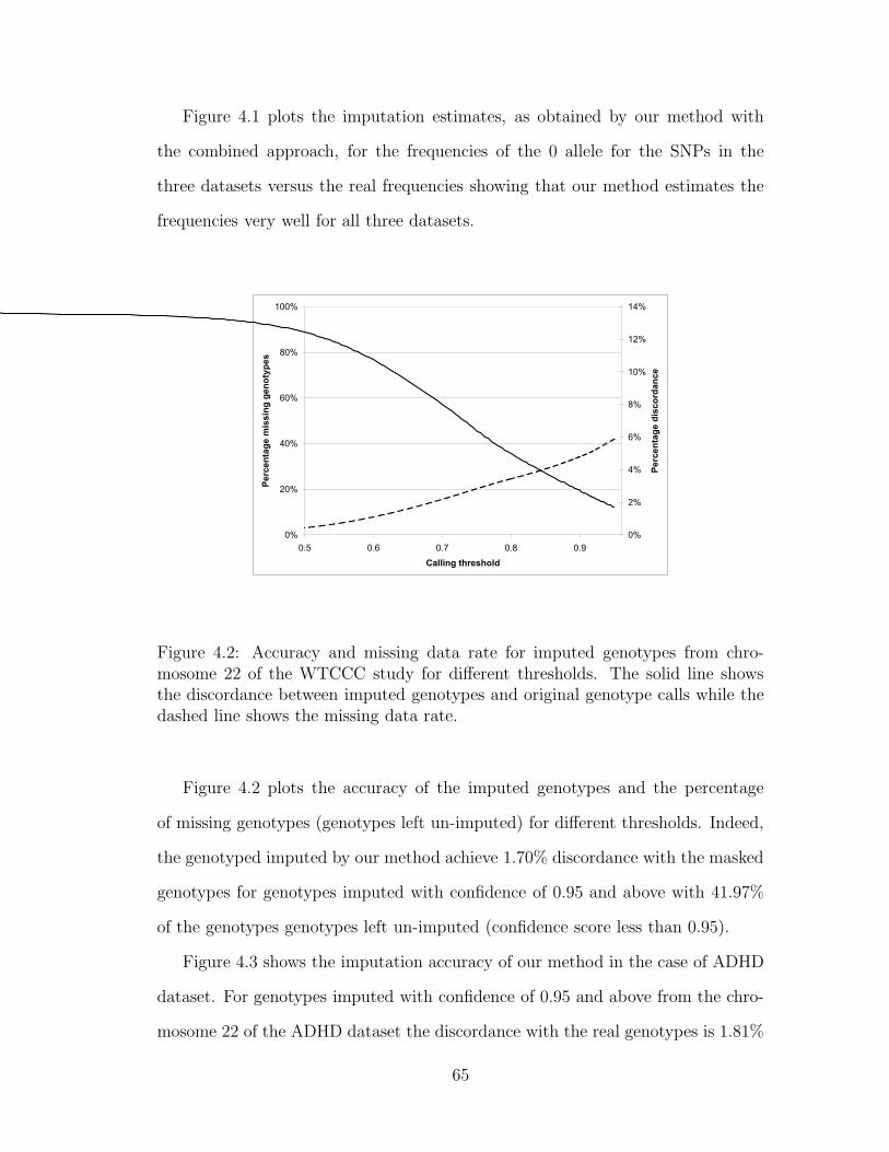
Figure 4.1 plots the imputation estimates, as obtained by our method with
the combined approach, for the frequencies of the 0 allele for the SNPs in the
three datasets versus the real frequencies showing that our method estimates the
frequencies very well for all three datasets.
0%
20%
40%
60%
80%
100%
0.5 0.6 0.7 0.8 0.9
Calling threshold
Perc
en
tag
e m
issin
g g
en
oty
pes
0%
2%
4%
6%
8%
10%
12%
14%
Pe
rce
nta
ge
dis
co
rda
nc
eFigure 4.2: Accuracy and missing data rate for imputed genotypes from chro-mosome 22 of the WTCCC study for different thresholds. The solid line showsthe discordance between imputed genotypes and original genotype calls while thedashed line shows the missing data rate.
Figure 4.2 plots the accuracy of the imputed genotypes and the percentage
of missing genotypes (genotypes left un-imputed) for different thresholds. Indeed,
the genotyped imputed by our method achieve 1.70% discordance with the masked
genotypes for genotypes imputed with confidence of 0.95 and above with 41.97%
of the genotypes genotypes left un-imputed (confidence score less than 0.95).
Figure 4.3 shows the imputation accuracy of our method in the case of ADHD
dataset. For genotypes imputed with confidence of 0.95 and above from the chro-
mosome 22 of the ADHD dataset the discordance with the real genotypes is 1.81%
65
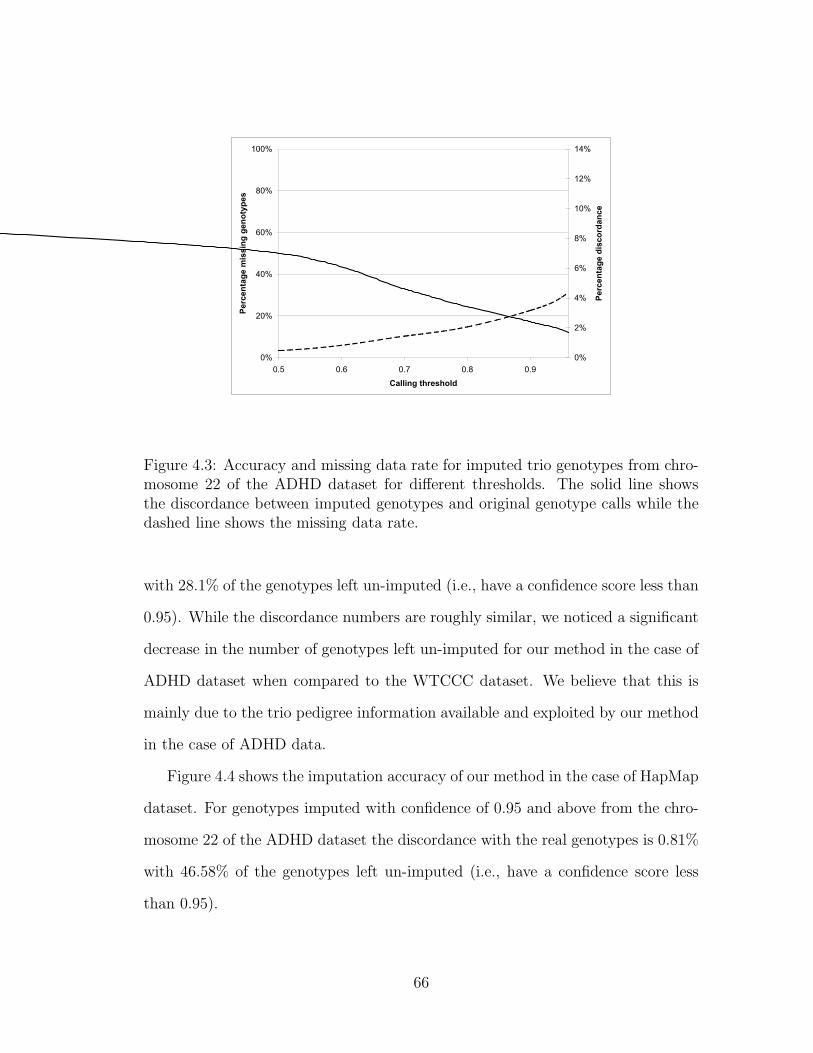
0%
20%
40%
60%
80%
100%
0.5 0.6 0.7 0.8 0.9
Calling threshold
Perc
en
tag
e m
issin
g g
en
oty
pes
0%
2%
4%
6%
8%
10%
12%
14%
Pe
rce
nta
ge
dis
co
rda
nc
e
Figure 4.3: Accuracy and missing data rate for imputed trio genotypes from chro-mosome 22 of the ADHD dataset for different thresholds. The solid line showsthe discordance between imputed genotypes and original genotype calls while thedashed line shows the missing data rate.
with 28.1% of the genotypes left un-imputed (i.e., have a confidence score less than
0.95). While the discordance numbers are roughly similar, we noticed a significant
decrease in the number of genotypes left un-imputed for our method in the case of
ADHD dataset when compared to the WTCCC dataset. We believe that this is
mainly due to the trio pedigree information available and exploited by our method
in the case of ADHD data.
Figure 4.4 shows the imputation accuracy of our method in the case of HapMap
dataset. For genotypes imputed with confidence of 0.95 and above from the chro-
mosome 22 of the ADHD dataset the discordance with the real genotypes is 0.81%
with 46.58% of the genotypes left un-imputed (i.e., have a confidence score less
than 0.95).
66
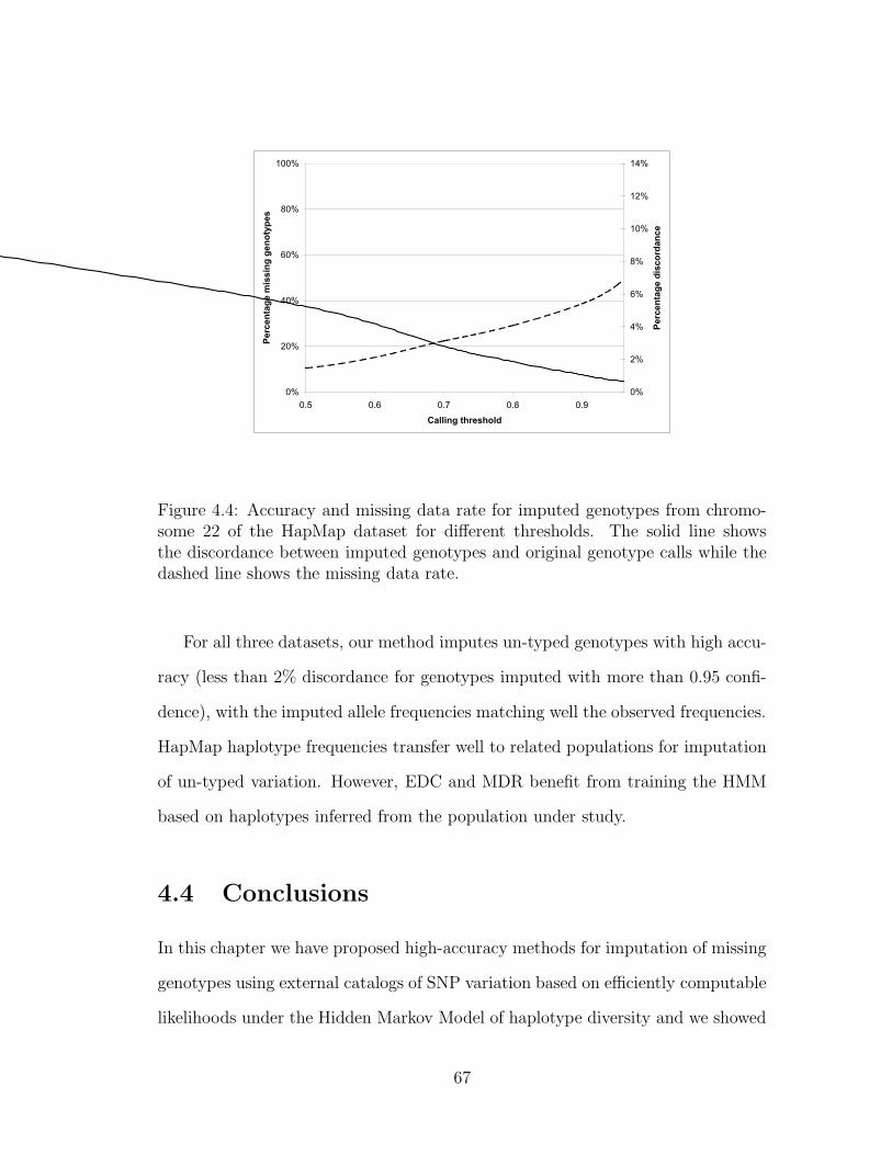
0%
20%
40%
60%
80%
100%
0.5 0.6 0.7 0.8 0.9
Calling threshold
Perc
en
tag
e m
issin
g g
en
oty
pes
0%
2%
4%
6%
8%
10%
12%
14%
Perc
en
tag
e d
isco
rdan
ce
Figure 4.4: Accuracy and missing data rate for imputed genotypes from chromo-some 22 of the HapMap dataset for different thresholds. The solid line showsthe discordance between imputed genotypes and original genotype calls while thedashed line shows the missing data rate.
For all three datasets, our method imputes un-typed genotypes with high accu-
racy (less than 2% discordance for genotypes imputed with more than 0.95 confi-
dence), with the imputed allele frequencies matching well the observed frequencies.
HapMap haplotype frequencies transfer well to related populations for imputation
of un-typed variation. However, EDC and MDR benefit from training the HMM
based on haplotypes inferred from the population under study.
4.4 Conclusions
In this chapter we have proposed high-accuracy methods for imputation of missing
genotypes using external catalogs of SNP variation based on efficiently computable
likelihoods under the Hidden Markov Model of haplotype diversity and we showed
67
how to efficiently extend our methods to handle complex pedigrees.
The error detection and correction (extending the error correction methods of
[30]) and the imputation methods presented in this chapter have been implemented
in a software package for Genotype Error Detection and Imputation (GEDI). With
a runtime that scales linearly both in the number of markers and the number of
typed individuals, GEDI is able to handle very large datasets while achieving
high accuracy rates for both error detection and imputation. The runtime of
our methods scales linearly with the number of trios and SNP loci, making them
appropriate for handling the datasets generated by current large-scale association
studies. The need for such methods is expected to increase in the future as genotype
analysis methods shift towards the use of haplotypes.
As future work, we are exploring the integration of population-level haplotype
frequency information with typing confidence scores for further improvements in
error detection and missing data recovery.
68
Chapter 5
A Comparison of Species
Identification Methods for DNA
Barcoding
Recently, DNA barcoding has been proposed as a tool for helping taxonomists in dif-
ferentiating species (http://www.barcoding.si.edu). According to the accepted
definition, DNA Barcoding is the use of a short DNA sequence from a standardized
region of the genome to help discover, characterize, and distinguish species, having
the main goal of creating a fingerprint for species. These short DNA sequences,
also called DNA barcodes, are very short relative to the entire genome and can be
obtained reasonably quickly and cheaply thus enabling a very cost-effective species
identification. The use of DNA barcodes for rapid species identification relies on
the assumption that the rate of evolution of short gene regions produces clear
interspecific sequence divergence while it maintains a low intraspecific sequence
variability. A mitochondrial gene region of 648 base pairs from the cytochrome c
oxidase subunit 1(COI) is emerging as the standard DNA barcode for almost all
1The results presented in this chapter are part of ongoing joint work with S. Gusev, S. Kentros,J. Lindsay and I. Mandoiu.
69
groups of higher animals [28, 55]. The large number of recently published stud-
ies shows the potential of DNA-barcoding as a cost-effective standard for rapid
species identification [41]. Several public barcode repositories such as the Barcode
of Life Data Systems (BOLD) database [52] are currently being developed. As
the size of these databases is increasing exponentially, BOLD already holds over
250k barcodes spanning 28k species, there is a strong need for scalable algorithms
to perform the assignment of new specimens to already cataloged species and to
further analyze the biological variability and its distribution within and among
species.
Many methods for species identification have been proposed, ranging from us-
ing a simple distance between sequences to constructing evolutionary trees. These
methods have been proposed within the context of independent studies and rela-
tively no work has been done to benchmark these methods. In this chapter we are
trying to fill in this gap by presenting a comprehensive methodology for comparing
different algorithms for species identification. Besides assessing the accuracy and
scalability of individual methods on real well-known datasets, we also study the
effect that the number of species, number of sampled specimens per species, and
the barcode length has on the identification accuracy. We are mainly concerned
with finding the required properties that a reference database should have in order
to obtain accurate and reliable identifications. In our assessment we vary the size
and quality of the database to detect the optimal parameters required for each
method. In this chapter we distinguish among three main classes of methods:
distance-based, that use a distance between barcodes to detect closest matches
in the database, tree-based, that rely on constructing a phylogenetic tree to help
the identification, and statistical model-based methods that define models for in-
traspecific variability and give probabilities for species memberships.
The rest of this chapter is organized as follows. We start by describing three
70
main classes of methods for species identification and we perform an initial com-
parison of the methods within each class on several well-known datasets. In a
second step, out of each class of methods, we pick a representative for which we
will assess the effect of the repository size on the identification accuracy.
5.1 Methods
We distinguish between three main classes of methods for species identification.
The first class contains methods that rely on defining a distance between barcodes
and then use this distance to find the closest match in the database, e.g. BOLD-
IDS [52] and TaxI [59]. The distance-based methods are usually very fast since
they involve only a series of distance computations between the query barcode
and the barcodes in the database. The downside is that they lack meaningful
confidence measures as showed in [17]. The second class of methods we present
here are tree-based methods that basically rely on building a phylogenetic tree for
the barcodes in the database plus the new barcode and assign the new barcode
to the closest neighbor in the tree, e.g. Meyers and Paulay [40]. These methods
have the deficiency of not scaling very well with the size of the database. The
third class of methods we describe are the probabilistic model based methods that
use a probabilistic model for finding the correct species, e.g. likelihood ratio test
of Nielsen and Matz [44]. While not as scalable as the distance-based methods,
the probabilistic methods have the advantage of providing meaningful statistical
significance measures.
5.1.1 Distance based methods
In this section we present algorithms for species identification that employ a dis-
tance between sequences. The main idea behind these methods is to assign the
71
unknown specimen to the species in the database that shows the least divergence;
usually a threshold is employed to check that the divergence is low enough. We
distinguish among several methods, depending on the used distance.
Hamming distance. The Hamming distance between two aligned barcodes is
defined as the number of positions where the two sequences have different nu-
cleotides. The new barcode is assigned to the species containing the closest se-
quence (MIN-HD) or to the specie with minimum average distance (AVG-HD).
MIN-HD is similar to the BOLD Identification System (BOLD-IDS) [52] since
BOLD-IDS assigns the query barcode to the species with the closest sequence in
the database. If the first 20 closest barcodes to the query sequence belong to dif-
ferent species then BOLD-IDS does not provide an identification at a species level
but a higher taxonomic unit (e.g. genus level identification).
Aminoacid similarity. After translating barcodes to aminoacid sequences a
pairwise similarity scores using the Blosum62 [29] matrix is computed. Then, the
new barcode is assigned to the species containing the highest similarity sequence
(MAX-AA-SIM) or with maximum average similarity (AVG-AA-SIM).
Convex-score similarity. The similarity score between two aligned barcode
sequences is determined from the positions where the two sequences have matching
nucleotides by summing the contributions of consecutive runs of matches, where
the contribution of a run is convexly increasing with its length. A new sequence is
assigned to the species containing the highest scoring sequence (MAX-CS-SIM).
Trinucleotide frequency. For each species we compute the vector of trinucleotide
frequencies, and the new sequence is assigned to the species whose frequency vector
is closest in Euclidian distance (MIN-3FREQ).
Combined method. We also implemented a simple voting scheme in which the
new barcode is assigned to the species for which the majority of the previously
described methods agree upon.
72
5.1.2 Tree-based methods
A relatively, novel concept in DNA barcoding is using a phylogenetic tree in guiding
the barcoding algorithm to assist in categorizing unknown sequences. Phylogenies
illustrate evolutionary interrelationships within a set of individuals which have
a common ancestor. Speciation events in organism evolution are represented by
multiple out-going branches from one common ancestral node. Such nodes can be
used in distinguishing the resultant subtaxa. Formally, a phylogenetic tree used
in DNA barcoding can be supplied from known biological data or re-created using
known sequences and various clustering techniques. Most of the works in this area
use the Neighbor Joining (NJ) method of [53] for reconstructing phylogenetic trees
from evolutionary distance data because of its robustness and scalability. The main
principle employed in the NJ-method is to find pairs of neighbors that minimize
the total branch length at each stage of clustering.
Exemplar Neighbor-Joining. The first tree-based method we present in this
section is the tree-based species identification proposed in [40]. In a first step one
exemplar from each species in the repository is chosen as the reference “barcode”
exemplar for that respective species. In the second step a NJ tree is build for
the exemplar barcodes and the new query barcode with unknown species. The
query barcode is assigned to the species of the closes barcode in the reconstructed
tree. Since in [40] the method of choosing the exemplar barcode is left ambiguous,
in our implementation we pick a barcode at random as a species exemplar. As
this algorithm requires the phylogenetic tree to be reconstructed for every query
barcode, its runtime is dependent on the size of the repository, and on the number
of query barcodes being identified.
Profile Neighbor-Joining. To address the possible short comings of using only
one barcode as exemplar for each species and improve the repeat neighbor-joining
73
exemplar technique we extended the algorithm to utilize a sequence profile for each
species instead of exemplar barcodes. The assumption is that using a sequence
profile rather than only one barcode will improve the accuracy of the NJ method.
Phylogenetic Traversal. A major drawback of the previously described tree-
based methods is the fact that a new tree needs to be constructed for each new
query barcode. We have devised an algorithm that reconstructs a phylogenetic NJ
tree only one time for the species in the repository. In the second step, the species of
the query barcode is found by a top-down transversal within this phylogenetic tree.
In order to take advantage of all available information, we build the tree based on
species profiles rather than exemplar barcodes. In the second step, for each internal
node in the reconstructed tree, we find a set of the k most discriminative positions
for the two children. An ideal discriminative position is one in which character 1
appears 100% in one child and as character 2 in all the barcodes corresponding to
the other child. However, since such characters are rarely present, we find the k
most most divergent positions in the children nodes, where the power of character
i of discriminating two taxonomic groups S1 and S2 is computed as follows:
w(i, S1, S2) =∑
x∈{A,C,T,G}
max{S1 ,S2}{Count(i, x, S1), Count(i, x, S2)}
Size(S1) + Size(S2)(5.1)
where Count(i, x, S1) is the number of times we observe nucleotide x at position
i in the barcodes of S1. Intuitively, w(i, S1, S2) measures the number of correct
assignments, if the barcodes b ∈ S1 ∪ S2 are assigned to the taxonomic group
with highest number of occurrences of b[i] at locus i. A similar method is used
in [2] to identify most discriminating substrings rather than characters. Since the
tree-traversal is done in linear time and it is only dependent on the height of the
tree, the algorithmic complexity is much lower than the previous methods that
require the regeneration of the tree for each query barcode, dramatically reducing
74
the runtime.
5.1.3 Probabilistic Model-based Methods
Several statistical approaches, e.g. the likelihood ratio test of Matz and Nielsen
[44] have been proposed for species identification; however, these methods are
impractical for even small sized datasets due to their computational complexity.
In this section we are going to present methods for species identification that rely
on building simpler statistical models for representing the intraspecific variability
that yield scalable methods capable of handling large barcode datasets.
Within our proposed model-based framework we are going to build a model
for each species in the database. Secondly, we compute the probability of the new
barcode belonging to each species model in the database and assign it to the most
probable species. Since the barcodes in the database have non uniform lengths and
cover different regions of the COI gene the membership probabilities are not always
comparable, the longer the barcode the smaller the probability. We overcome this
problem by having a background model that represents the variability observed in
all the barcodes in the database. We normalize each membership probability by
the probability under the background model. Finally, the new barcode is assigned
to the species that maximizes this normalized probability. Depending on how we
model the variability within each species, we distinguish between several methods.
Positional Weight Matrix Model. For each species we compute a Positional
Weight Matrix (PWM) that gives, for each loci, the probability of seeing a nu-
cleotide in that species at that locus. For each new sequence we compute the
probability of being generated according to the PWM of each species, and select
the species that gives the highest probability (MAX-PWM). The major drawback
of this model is the assumption of independence among loci, assumption that is
clearly not suited for coding regions such as the mitochondrial gene region used as
75
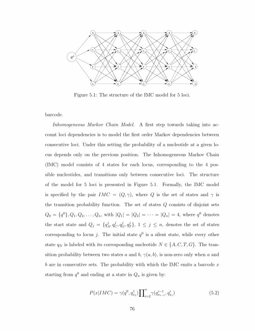
���������������������������������������������������������������������������������������������������������������������
���������������������������������������������������������������������������������������������������������������������
����������������������������������������������������������������������������������������������������������������������������������������������������������������������������������������������������������������������������������������������������������������������������������������������������������������������������������������������������������������������������
����������������������������������������������������������������������������������������������������������������������������������������������������������������������������������������������������������������������������������������������������������������������������������������������������������������������������������������������������������������������������
������������������������������������������������������������������������������������������������������������������������������������������������������������������������������������������������������������������������������������������
������������������������������������������������������������������������������������������������������������������������������������������������������������������������������������������������������������������������������������������
����������������������������������������������������������������������������������������������������������������������������������������������������������������������������������������������������������������������������������������������������������������������������������������������������������������������������������������������������������������������������
����������������������������������������������������������������������������������������������������������������������������������������������������������������������������������������������������������������������������������������������������������������������������������������������������������������������������������������������������������������������������
������������������������������������������������������������������������������������������������������������������
������������������������������������������������������������������������������������������������������������������
���������������������������������������������������������������������������������������������������������������������
���������������������������������������������������������������������������������������������������������������������
� � � � � � � � � � � � � � � � � � � � � � � � � � � � � � � � � � � � � � � � � � � � � � � �
��������������������������������������������������������������������������������������������������������
����������������������������������������������������������������������������������������
����������������������������������������������������������������������������������������
������������������������������������������������������������������������������������������������������������������������������������������������������������������������������������������������������������������������������������������
������������������������������������������������������������������������������������������������������������������������������������������������������������������������������������������������������������������������������������������
���������������������������������������������������������������������������������������������������������������������
���������������������������������������������������������������������������������������������������������������������
����������������������������������������������������������������������������������������������������������������������������������
����������������������������������������������������������������������������������������������������������������������������������
������������������������������������������������������������������������������������������������������������������������������������������������������������������������������������������������������������������������������������������
������������������������������������������������������������������������������������������������������������������������������������������������������������������������������������������������������������������������������������������
���������������������������������������������������������������������������������������������������������������������
���������������������������������������������������������������������������������������������������������������������
����������������������������������������������������������������������������������������������������������������������������������������������������������������������������������������������������������������������������������������������������������������������������������������������������������������������������������������������������������������������������
����������������������������������������������������������������������������������������������������������������������������������������������������������������������������������������������������������������������������������������������������������������������������������������������������������������������������������������������������������������������������
������������������������������������������������������������������������������������������������������������������������������������������������������������������������������������������������������������������������������������������
������������������������������������������������������������������������������������������������������������������������������������������������������������������������������������������������������������������������������������������
����������������������������������������������������������������������������������������������������������������������������������������������������������������������������������������������������������������������������������������������������������������������������������������������������������������������������������������������������������������������������
� � � � � � � � � � � � � � � � � � � � � � � � � � � � � � � � � � � � � � � � � � � � � � � � � � � � � � � � � � � � � � � � � � � � � � � � � � � � � � � � � � � � � � � � � � � � � � � � � � � � � � � � � � � � � � � � � � � � � � � � � � � � � � � � � � � � � � � � � � � � � � � � � � � � � � � � � � � � � � � � � � � � � � � �
!�!�!�!�!�!�!!�!�!�!�!�!�!!�!�!�!�!�!�!!�!�!�!�!�!�!!�!�!�!�!�!�!!�!�!�!�!�!�!!�!�!�!�!�!�!!�!�!�!�!�!�!!�!�!�!�!�!�!!�!�!�!�!�!�!!�!�!�!�!�!�!!�!�!�!�!�!�!!�!�!�!�!�!�!!�!�!�!�!�!�!!�!�!�!�!�!�!!�!�!�!�!�!�!!�!�!�!�!�!�!!�!�!�!�!�!�!!�!�!�!�!�!�!
"�"�"�"�"�"�""�"�"�"�"�"�""�"�"�"�"�"�""�"�"�"�"�"�""�"�"�"�"�"�""�"�"�"�"�"�""�"�"�"�"�"�""�"�"�"�"�"�""�"�"�"�"�"�""�"�"�"�"�"�""�"�"�"�"�"�""�"�"�"�"�"�""�"�"�"�"�"�""�"�"�"�"�"�""�"�"�"�"�"�""�"�"�"�"�"�""�"�"�"�"�"�""�"�"�"�"�"�""�"�"�"�"�"�"
#�#�#�#�#�#�##�#�#�#�#�#�##�#�#�#�#�#�##�#�#�#�#�#�##�#�#�#�#�#�##�#�#�#�#�#�##�#�#�#�#�#�##�#�#�#�#�#�##�#�#�#�#�#�#
$�$�$�$�$�$�$$�$�$�$�$�$�$$�$�$�$�$�$�$$�$�$�$�$�$�$$�$�$�$�$�$�$$�$�$�$�$�$�$$�$�$�$�$�$�$$�$�$�$�$�$�$$�$�$�$�$�$�$
%�%�%�%�%�%�%%�%�%�%�%�%�%%�%�%�%�%�%�%%�%�%�%�%�%�%%�%�%�%�%�%�%%�%�%�%�%�%�%%�%�%�%�%�%�%%�%�%�%�%�%�%
&�&�&�&�&�&�&&�&�&�&�&�&�&&�&�&�&�&�&�&&�&�&�&�&�&�&&�&�&�&�&�&�&&�&�&�&�&�&�&&�&�&�&�&�&�&&�&�&�&�&�&�&
'�'�'�'�'�''�'�'�'�'�''�'�'�'�'�''�'�'�'�'�''�'�'�'�'�''�'�'�'�'�''�'�'�'�'�''�'�'�'�'�'
(�(�(�(�(�((�(�(�(�(�((�(�(�(�(�((�(�(�(�(�((�(�(�(�(�((�(�(�(�(�((�(�(�(�(�((�(�(�(�(�(
)�)�)�)�)�)�))�)�)�)�)�)�))�)�)�)�)�)�))�)�)�)�)�)�))�)�)�)�)�)�))�)�)�)�)�)�))�)�)�)�)�)�))�)�)�)�)�)�))�)�)�)�)�)�))�)�)�)�)�)�))�)�)�)�)�)�))�)�)�)�)�)�))�)�)�)�)�)�))�)�)�)�)�)�))�)�)�)�)�)�))�)�)�)�)�)�))�)�)�)�)�)�))�)�)�)�)�)�)
*�*�*�*�*�*�**�*�*�*�*�*�**�*�*�*�*�*�**�*�*�*�*�*�**�*�*�*�*�*�**�*�*�*�*�*�**�*�*�*�*�*�**�*�*�*�*�*�**�*�*�*�*�*�**�*�*�*�*�*�**�*�*�*�*�*�**�*�*�*�*�*�**�*�*�*�*�*�**�*�*�*�*�*�**�*�*�*�*�*�**�*�*�*�*�*�**�*�*�*�*�*�**�*�*�*�*�*�*
+�+�+�+�+�+�++�+�+�+�+�+�++�+�+�+�+�+�++�+�+�+�+�+�++�+�+�+�+�+�++�+�+�+�+�+�++�+�+�+�+�+�++�+�+�+�+�+�++�+�+�+�+�+�+
,�,�,�,�,�,�,,�,�,�,�,�,�,,�,�,�,�,�,�,,�,�,�,�,�,�,,�,�,�,�,�,�,,�,�,�,�,�,�,,�,�,�,�,�,�,,�,�,�,�,�,�,,�,�,�,�,�,�,
-�-�-�-�-�-�--�-�-�-�-�-�--�-�-�-�-�-�--�-�-�-�-�-�--�-�-�-�-�-�--�-�-�-�-�-�--�-�-�-�-�-�--�-�-�-�-�-�--�-�-�-�-�-�--�-�-�-�-�-�-
.�.�.�.�.�.�..�.�.�.�.�.�..�.�.�.�.�.�..�.�.�.�.�.�..�.�.�.�.�.�..�.�.�.�.�.�..�.�.�.�.�.�..�.�.�.�.�.�..�.�.�.�.�.�..�.�.�.�.�.�.
/�/�/�/�/�/�//�/�/�/�/�/�//�/�/�/�/�/�//�/�/�/�/�/�//�/�/�/�/�/�//�/�/�/�/�/�//�/�/�/�/�/�//�/�/�/�/�/�//�/�/�/�/�/�//�/�/�/�/�/�//�/�/�/�/�/�//�/�/�/�/�/�//�/�/�/�/�/�//�/�/�/�/�/�//�/�/�/�/�/�//�/�/�/�/�/�//�/�/�/�/�/�//�/�/�/�/�/�/
0�0�0�0�0�0�00�0�0�0�0�0�00�0�0�0�0�0�00�0�0�0�0�0�00�0�0�0�0�0�00�0�0�0�0�0�00�0�0�0�0�0�00�0�0�0�0�0�00�0�0�0�0�0�00�0�0�0�0�0�00�0�0�0�0�0�00�0�0�0�0�0�00�0�0�0�0�0�00�0�0�0�0�0�00�0�0�0�0�0�00�0�0�0�0�0�00�0�0�0�0�0�00�0�0�0�0�0�0
1�1�1�1�1�1�11�1�1�1�1�1�11�1�1�1�1�1�11�1�1�1�1�1�11�1�1�1�1�1�11�1�1�1�1�1�11�1�1�1�1�1�11�1�1�1�1�1�11�1�1�1�1�1�1
2�2�2�2�2�2�22�2�2�2�2�2�22�2�2�2�2�2�22�2�2�2�2�2�22�2�2�2�2�2�22�2�2�2�2�2�22�2�2�2�2�2�22�2�2�2�2�2�22�2�2�2�2�2�2
3�3�3�3�3�3�33�3�3�3�3�3�33�3�3�3�3�3�33�3�3�3�3�3�33�3�3�3�3�3�33�3�3�3�3�3�33�3�3�3�3�3�33�3�3�3�3�3�33�3�3�3�3�3�33�3�3�3�3�3�33�3�3�3�3�3�33�3�3�3�3�3�33�3�3�3�3�3�33�3�3�3�3�3�33�3�3�3�3�3�33�3�3�3�3�3�33�3�3�3�3�3�33�3�3�3�3�3�33�3�3�3�3�3�33�3�3�3�3�3�33�3�3�3�3�3�33�3�3�3�3�3�33�3�3�3�3�3�33�3�3�3�3�3�33�3�3�3�3�3�33�3�3�3�3�3�33�3�3�3�3�3�33�3�3�3�3�3�3
4�4�4�4�4�4�44�4�4�4�4�4�44�4�4�4�4�4�44�4�4�4�4�4�44�4�4�4�4�4�44�4�4�4�4�4�44�4�4�4�4�4�44�4�4�4�4�4�44�4�4�4�4�4�44�4�4�4�4�4�44�4�4�4�4�4�44�4�4�4�4�4�44�4�4�4�4�4�44�4�4�4�4�4�44�4�4�4�4�4�44�4�4�4�4�4�44�4�4�4�4�4�44�4�4�4�4�4�44�4�4�4�4�4�44�4�4�4�4�4�44�4�4�4�4�4�44�4�4�4�4�4�44�4�4�4�4�4�44�4�4�4�4�4�44�4�4�4�4�4�44�4�4�4�4�4�44�4�4�4�4�4�44�4�4�4�4�4�4
5�5�5�5�5�5�55�5�5�5�5�5�55�5�5�5�5�5�55�5�5�5�5�5�55�5�5�5�5�5�55�5�5�5�5�5�55�5�5�5�5�5�55�5�5�5�5�5�55�5�5�5�5�5�55�5�5�5�5�5�55�5�5�5�5�5�55�5�5�5�5�5�55�5�5�5�5�5�55�5�5�5�5�5�55�5�5�5�5�5�55�5�5�5�5�5�55�5�5�5�5�5�55�5�5�5�5�5�5
6�6�6�6�6�6�66�6�6�6�6�6�66�6�6�6�6�6�66�6�6�6�6�6�66�6�6�6�6�6�66�6�6�6�6�6�66�6�6�6�6�6�66�6�6�6�6�6�66�6�6�6�6�6�66�6�6�6�6�6�66�6�6�6�6�6�66�6�6�6�6�6�66�6�6�6�6�6�66�6�6�6�6�6�66�6�6�6�6�6�66�6�6�6�6�6�66�6�6�6�6�6�66�6�6�6�6�6�6
7�7�7�7�7�7�77�7�7�7�7�7�77�7�7�7�7�7�77�7�7�7�7�7�77�7�7�7�7�7�77�7�7�7�7�7�77�7�7�7�7�7�77�7�7�7�7�7�77�7�7�7�7�7�77�7�7�7�7�7�77�7�7�7�7�7�77�7�7�7�7�7�77�7�7�7�7�7�77�7�7�7�7�7�77�7�7�7�7�7�77�7�7�7�7�7�77�7�7�7�7�7�77�7�7�7�7�7�77�7�7�7�7�7�77�7�7�7�7�7�77�7�7�7�7�7�77�7�7�7�7�7�77�7�7�7�7�7�77�7�7�7�7�7�77�7�7�7�7�7�77�7�7�7�7�7�77�7�7�7�7�7�77�7�7�7�7�7�7
8�8�8�8�8�8�88�8�8�8�8�8�88�8�8�8�8�8�88�8�8�8�8�8�88�8�8�8�8�8�88�8�8�8�8�8�88�8�8�8�8�8�88�8�8�8�8�8�88�8�8�8�8�8�88�8�8�8�8�8�88�8�8�8�8�8�88�8�8�8�8�8�88�8�8�8�8�8�88�8�8�8�8�8�88�8�8�8�8�8�88�8�8�8�8�8�88�8�8�8�8�8�88�8�8�8�8�8�88�8�8�8�8�8�88�8�8�8�8�8�88�8�8�8�8�8�88�8�8�8�8�8�88�8�8�8�8�8�88�8�8�8�8�8�88�8�8�8�8�8�88�8�8�8�8�8�88�8�8�8�8�8�88�8�8�8�8�8�8
9�9�9�9�9�9�99�9�9�9�9�9�99�9�9�9�9�9�99�9�9�9�9�9�99�9�9�9�9�9�99�9�9�9�9�9�99�9�9�9�9�9�99�9�9�9�9�9�99�9�9�9�9�9�99�9�9�9�9�9�99�9�9�9�9�9�99�9�9�9�9�9�99�9�9�9�9�9�99�9�9�9�9�9�99�9�9�9�9�9�99�9�9�9�9�9�99�9�9�9�9�9�99�9�9�9�9�9�99�9�9�9�9�9�9
:�:�:�:�:�:�::�:�:�:�:�:�::�:�:�:�:�:�::�:�:�:�:�:�::�:�:�:�:�:�::�:�:�:�:�:�::�:�:�:�:�:�::�:�:�:�:�:�::�:�:�:�:�:�::�:�:�:�:�:�::�:�:�:�:�:�::�:�:�:�:�:�::�:�:�:�:�:�::�:�:�:�:�:�::�:�:�:�:�:�::�:�:�:�:�:�::�:�:�:�:�:�::�:�:�:�:�:�::�:�:�:�:�:�:
;�;�;�;�;�;�;;�;�;�;�;�;�;;�;�;�;�;�;�;;�;�;�;�;�;�;;�;�;�;�;�;�;;�;�;�;�;�;�;;�;�;�;�;�;�;;�;�;�;�;�;�;;�;�;�;�;�;�;
<�<�<�<�<�<�<<�<�<�<�<�<�<<�<�<�<�<�<�<<�<�<�<�<�<�<<�<�<�<�<�<�<<�<�<�<�<�<�<<�<�<�<�<�<�<<�<�<�<�<�<�<<�<�<�<�<�<�<
=�=�=�=�=�=�==�=�=�=�=�=�==�=�=�=�=�=�==�=�=�=�=�=�==�=�=�=�=�=�==�=�=�=�=�=�==�=�=�=�=�=�==�=�=�=�=�=�=
>�>�>�>�>�>�>>�>�>�>�>�>�>>�>�>�>�>�>�>>�>�>�>�>�>�>>�>�>�>�>�>�>>�>�>�>�>�>�>>�>�>�>�>�>�>>�>�>�>�>�>�>
?�?�?�?�?�??�?�?�?�?�??�?�?�?�?�??�?�?�?�?�??�?�?�?�?�??�?�?�?�?�??�?�?�?�?�??�?�?�?�?�?
@�@�@�@�@�@@�@�@�@�@�@@�@�@�@�@�@@�@�@�@�@�@@�@�@�@�@�@@�@�@�@�@�@@�@�@�@�@�@@�@�@�@�@�@
A�A�A�A�A�A�AA�A�A�A�A�A�AA�A�A�A�A�A�AA�A�A�A�A�A�AA�A�A�A�A�A�AA�A�A�A�A�A�AA�A�A�A�A�A�AA�A�A�A�A�A�AA�A�A�A�A�A�AA�A�A�A�A�A�AA�A�A�A�A�A�AA�A�A�A�A�A�AA�A�A�A�A�A�AA�A�A�A�A�A�AA�A�A�A�A�A�AA�A�A�A�A�A�AA�A�A�A�A�A�AA�A�A�A�A�A�A
B�B�B�B�B�B�BB�B�B�B�B�B�BB�B�B�B�B�B�BB�B�B�B�B�B�BB�B�B�B�B�B�BB�B�B�B�B�B�BB�B�B�B�B�B�BB�B�B�B�B�B�BB�B�B�B�B�B�BB�B�B�B�B�B�BB�B�B�B�B�B�BB�B�B�B�B�B�BB�B�B�B�B�B�BB�B�B�B�B�B�BB�B�B�B�B�B�BB�B�B�B�B�B�BB�B�B�B�B�B�BB�B�B�B�B�B�B
C�C�C�C�C�C�CC�C�C�C�C�C�CC�C�C�C�C�C�CC�C�C�C�C�C�CC�C�C�C�C�C�CC�C�C�C�C�C�CC�C�C�C�C�C�CC�C�C�C�C�C�CC�C�C�C�C�C�C
D�D�D�D�D�D�DD�D�D�D�D�D�DD�D�D�D�D�D�DD�D�D�D�D�D�DD�D�D�D�D�D�DD�D�D�D�D�D�DD�D�D�D�D�D�DD�D�D�D�D�D�DD�D�D�D�D�D�D
E�E�E�E�E�E�EE�E�E�E�E�E�EE�E�E�E�E�E�EE�E�E�E�E�E�EE�E�E�E�E�E�EE�E�E�E�E�E�EE�E�E�E�E�E�EE�E�E�E�E�E�EE�E�E�E�E�E�EE�E�E�E�E�E�E
F�F�F�F�F�F�FF�F�F�F�F�F�FF�F�F�F�F�F�FF�F�F�F�F�F�FF�F�F�F�F�F�FF�F�F�F�F�F�FF�F�F�F�F�F�FF�F�F�F�F�F�FF�F�F�F�F�F�FF�F�F�F�F�F�F
G�G�G�G�G�G�GG�G�G�G�G�G�GG�G�G�G�G�G�GG�G�G�G�G�G�GG�G�G�G�G�G�GG�G�G�G�G�G�GG�G�G�G�G�G�GG�G�G�G�G�G�GG�G�G�G�G�G�GG�G�G�G�G�G�GG�G�G�G�G�G�GG�G�G�G�G�G�GG�G�G�G�G�G�GG�G�G�G�G�G�GG�G�G�G�G�G�GG�G�G�G�G�G�GG�G�G�G�G�G�GG�G�G�G�G�G�G
H�H�H�H�H�H�HH�H�H�H�H�H�HH�H�H�H�H�H�HH�H�H�H�H�H�HH�H�H�H�H�H�HH�H�H�H�H�H�HH�H�H�H�H�H�HH�H�H�H�H�H�HH�H�H�H�H�H�HH�H�H�H�H�H�HH�H�H�H�H�H�HH�H�H�H�H�H�HH�H�H�H�H�H�HH�H�H�H�H�H�HH�H�H�H�H�H�HH�H�H�H�H�H�HH�H�H�H�H�H�HH�H�H�H�H�H�H
I�I�I�I�I�I�II�I�I�I�I�I�II�I�I�I�I�I�II�I�I�I�I�I�II�I�I�I�I�I�II�I�I�I�I�I�II�I�I�I�I�I�II�I�I�I�I�I�II�I�I�I�I�I�I
J�J�J�J�J�J�JJ�J�J�J�J�J�JJ�J�J�J�J�J�JJ�J�J�J�J�J�JJ�J�J�J�J�J�JJ�J�J�J�J�J�JJ�J�J�J�J�J�JJ�J�J�J�J�J�JJ�J�J�J�J�J�J
K�K�K�K�K�K�KK�K�K�K�K�K�KK�K�K�K�K�K�KK�K�K�K�K�K�KK�K�K�K�K�K�KK�K�K�K�K�K�KK�K�K�K�K�K�KK�K�K�K�K�K�KK�K�K�K�K�K�KK�K�K�K�K�K�KK�K�K�K�K�K�KK�K�K�K�K�K�KK�K�K�K�K�K�KK�K�K�K�K�K�KK�K�K�K�K�K�KK�K�K�K�K�K�KK�K�K�K�K�K�KK�K�K�K�K�K�KK�K�K�K�K�K�KK�K�K�K�K�K�KK�K�K�K�K�K�KK�K�K�K�K�K�KK�K�K�K�K�K�KK�K�K�K�K�K�KK�K�K�K�K�K�KK�K�K�K�K�K�KK�K�K�K�K�K�KK�K�K�K�K�K�K
L�L�L�L�L�L�LL�L�L�L�L�L�LL�L�L�L�L�L�LL�L�L�L�L�L�LL�L�L�L�L�L�LL�L�L�L�L�L�LL�L�L�L�L�L�LL�L�L�L�L�L�LL�L�L�L�L�L�LL�L�L�L�L�L�LL�L�L�L�L�L�LL�L�L�L�L�L�LL�L�L�L�L�L�LL�L�L�L�L�L�LL�L�L�L�L�L�LL�L�L�L�L�L�LL�L�L�L�L�L�LL�L�L�L�L�L�LL�L�L�L�L�L�LL�L�L�L�L�L�LL�L�L�L�L�L�LL�L�L�L�L�L�LL�L�L�L�L�L�LL�L�L�L�L�L�LL�L�L�L�L�L�LL�L�L�L�L�L�LL�L�L�L�L�L�LL�L�L�L�L�L�L
M�M�M�M�M�M�MM�M�M�M�M�M�MM�M�M�M�M�M�MM�M�M�M�M�M�MM�M�M�M�M�M�MM�M�M�M�M�M�MM�M�M�M�M�M�MM�M�M�M�M�M�MM�M�M�M�M�M�MM�M�M�M�M�M�MM�M�M�M�M�M�MM�M�M�M�M�M�MM�M�M�M�M�M�MM�M�M�M�M�M�MM�M�M�M�M�M�MM�M�M�M�M�M�MM�M�M�M�M�M�MM�M�M�M�M�M�M
N�N�N�N�N�N�NN�N�N�N�N�N�NN�N�N�N�N�N�NN�N�N�N�N�N�NN�N�N�N�N�N�NN�N�N�N�N�N�NN�N�N�N�N�N�NN�N�N�N�N�N�NN�N�N�N�N�N�NN�N�N�N�N�N�NN�N�N�N�N�N�NN�N�N�N�N�N�NN�N�N�N�N�N�NN�N�N�N�N�N�NN�N�N�N�N�N�NN�N�N�N�N�N�NN�N�N�N�N�N�NN�N�N�N�N�N�N
O�O�O�O�O�O�OO�O�O�O�O�O�OO�O�O�O�O�O�OO�O�O�O�O�O�OO�O�O�O�O�O�OO�O�O�O�O�O�OO�O�O�O�O�O�OO�O�O�O�O�O�OO�O�O�O�O�O�OO�O�O�O�O�O�OO�O�O�O�O�O�OO�O�O�O�O�O�OO�O�O�O�O�O�OO�O�O�O�O�O�OO�O�O�O�O�O�OO�O�O�O�O�O�OO�O�O�O�O�O�OO�O�O�O�O�O�OO�O�O�O�O�O�OO�O�O�O�O�O�OO�O�O�O�O�O�OO�O�O�O�O�O�OO�O�O�O�O�O�OO�O�O�O�O�O�OO�O�O�O�O�O�OO�O�O�O�O�O�OO�O�O�O�O�O�OO�O�O�O�O�O�O
P�P�P�P�P�P�PP�P�P�P�P�P�PP�P�P�P�P�P�PP�P�P�P�P�P�PP�P�P�P�P�P�PP�P�P�P�P�P�PP�P�P�P�P�P�PP�P�P�P�P�P�PP�P�P�P�P�P�PP�P�P�P�P�P�PP�P�P�P�P�P�PP�P�P�P�P�P�PP�P�P�P�P�P�PP�P�P�P�P�P�PP�P�P�P�P�P�PP�P�P�P�P�P�PP�P�P�P�P�P�PP�P�P�P�P�P�PP�P�P�P�P�P�PP�P�P�P�P�P�PP�P�P�P�P�P�PP�P�P�P�P�P�PP�P�P�P�P�P�PP�P�P�P�P�P�PP�P�P�P�P�P�PP�P�P�P�P�P�PP�P�P�P�P�P�PP�P�P�P�P�P�P
Q�Q�Q�Q�Q�Q�QQ�Q�Q�Q�Q�Q�QQ�Q�Q�Q�Q�Q�QQ�Q�Q�Q�Q�Q�QQ�Q�Q�Q�Q�Q�QQ�Q�Q�Q�Q�Q�QQ�Q�Q�Q�Q�Q�QQ�Q�Q�Q�Q�Q�QQ�Q�Q�Q�Q�Q�QQ�Q�Q�Q�Q�Q�QQ�Q�Q�Q�Q�Q�QQ�Q�Q�Q�Q�Q�QQ�Q�Q�Q�Q�Q�QQ�Q�Q�Q�Q�Q�QQ�Q�Q�Q�Q�Q�QQ�Q�Q�Q�Q�Q�QQ�Q�Q�Q�Q�Q�QQ�Q�Q�Q�Q�Q�QQ�Q�Q�Q�Q�Q�Q
R�R�R�R�R�R�RR�R�R�R�R�R�RR�R�R�R�R�R�RR�R�R�R�R�R�RR�R�R�R�R�R�RR�R�R�R�R�R�RR�R�R�R�R�R�RR�R�R�R�R�R�RR�R�R�R�R�R�RR�R�R�R�R�R�RR�R�R�R�R�R�RR�R�R�R�R�R�RR�R�R�R�R�R�RR�R�R�R�R�R�RR�R�R�R�R�R�RR�R�R�R�R�R�RR�R�R�R�R�R�RR�R�R�R�R�R�RR�R�R�R�R�R�R
S�S�S�S�S�S�SS�S�S�S�S�S�SS�S�S�S�S�S�SS�S�S�S�S�S�SS�S�S�S�S�S�SS�S�S�S�S�S�SS�S�S�S�S�S�SS�S�S�S�S�S�SS�S�S�S�S�S�S
T�T�T�T�T�T�TT�T�T�T�T�T�TT�T�T�T�T�T�TT�T�T�T�T�T�TT�T�T�T�T�T�TT�T�T�T�T�T�TT�T�T�T�T�T�TT�T�T�T�T�T�TT�T�T�T�T�T�T
U�U�U�U�U�U�UU�U�U�U�U�U�UU�U�U�U�U�U�UU�U�U�U�U�U�UU�U�U�U�U�U�UU�U�U�U�U�U�UU�U�U�U�U�U�UU�U�U�U�U�U�U
V�V�V�V�V�V�VV�V�V�V�V�V�VV�V�V�V�V�V�VV�V�V�V�V�V�VV�V�V�V�V�V�VV�V�V�V�V�V�VV�V�V�V�V�V�VV�V�V�V�V�V�V
W�W�W�W�W�WW�W�W�W�W�WW�W�W�W�W�WW�W�W�W�W�WW�W�W�W�W�WW�W�W�W�W�WW�W�W�W�W�WW�W�W�W�W�W
X�X�X�X�X�XX�X�X�X�X�XX�X�X�X�X�XX�X�X�X�X�XX�X�X�X�X�XX�X�X�X�X�XX�X�X�X�X�XX�X�X�X�X�X
Y�Y�Y�Y�Y�Y�YY�Y�Y�Y�Y�Y�YY�Y�Y�Y�Y�Y�YY�Y�Y�Y�Y�Y�YY�Y�Y�Y�Y�Y�YY�Y�Y�Y�Y�Y�YY�Y�Y�Y�Y�Y�YY�Y�Y�Y�Y�Y�YY�Y�Y�Y�Y�Y�YY�Y�Y�Y�Y�Y�YY�Y�Y�Y�Y�Y�YY�Y�Y�Y�Y�Y�YY�Y�Y�Y�Y�Y�YY�Y�Y�Y�Y�Y�YY�Y�Y�Y�Y�Y�YY�Y�Y�Y�Y�Y�YY�Y�Y�Y�Y�Y�YY�Y�Y�Y�Y�Y�Y
Z�Z�Z�Z�Z�Z�ZZ�Z�Z�Z�Z�Z�ZZ�Z�Z�Z�Z�Z�ZZ�Z�Z�Z�Z�Z�ZZ�Z�Z�Z�Z�Z�ZZ�Z�Z�Z�Z�Z�ZZ�Z�Z�Z�Z�Z�ZZ�Z�Z�Z�Z�Z�ZZ�Z�Z�Z�Z�Z�ZZ�Z�Z�Z�Z�Z�ZZ�Z�Z�Z�Z�Z�ZZ�Z�Z�Z�Z�Z�ZZ�Z�Z�Z�Z�Z�ZZ�Z�Z�Z�Z�Z�ZZ�Z�Z�Z�Z�Z�ZZ�Z�Z�Z�Z�Z�ZZ�Z�Z�Z�Z�Z�ZZ�Z�Z�Z�Z�Z�Z
[�[�[�[�[�[�[[�[�[�[�[�[�[[�[�[�[�[�[�[[�[�[�[�[�[�[[�[�[�[�[�[�[[�[�[�[�[�[�[[�[�[�[�[�[�[[�[�[�[�[�[�[[�[�[�[�[�[�[[�[�[�[�[�[�[
\�\�\�\�\�\�\\�\�\�\�\�\�\\�\�\�\�\�\�\\�\�\�\�\�\�\\�\�\�\�\�\�\\�\�\�\�\�\�\\�\�\�\�\�\�\\�\�\�\�\�\�\\�\�\�\�\�\�\\�\�\�\�\�\�\
]�]�]�]�]�]�]]�]�]�]�]�]�]]�]�]�]�]�]�]]�]�]�]�]�]�]]�]�]�]�]�]�]]�]�]�]�]�]�]]�]�]�]�]�]�]]�]�]�]�]�]�]]�]�]�]�]�]�]]�]�]�]�]�]�]]�]�]�]�]�]�]]�]�]�]�]�]�]]�]�]�]�]�]�]]�]�]�]�]�]�]]�]�]�]�]�]�]]�]�]�]�]�]�]]�]�]�]�]�]�]]�]�]�]�]�]�]
^�^�^�^�^�^�^^�^�^�^�^�^�^^�^�^�^�^�^�^^�^�^�^�^�^�^^�^�^�^�^�^�^^�^�^�^�^�^�^^�^�^�^�^�^�^^�^�^�^�^�^�^^�^�^�^�^�^�^^�^�^�^�^�^�^^�^�^�^�^�^�^^�^�^�^�^�^�^^�^�^�^�^�^�^^�^�^�^�^�^�^^�^�^�^�^�^�^^�^�^�^�^�^�^^�^�^�^�^�^�^^�^�^�^�^�^�^
_�_�_�_�_�_�__�_�_�_�_�_�__�_�_�_�_�_�__�_�_�_�_�_�__�_�_�_�_�_�__�_�_�_�_�_�__�_�_�_�_�_�__�_�_�_�_�_�__�_�_�_�_�_�_
`�`�`�`�`�`�``�`�`�`�`�`�``�`�`�`�`�`�``�`�`�`�`�`�``�`�`�`�`�`�``�`�`�`�`�`�``�`�`�`�`�`�``�`�`�`�`�`�``�`�`�`�`�`�`
q0
A
G
T
C
G G G G
T T T T
A A A A
CCCC
Figure 5.1: The structure of the IMC model for 5 loci.
barcode.
Inhomogeneous Markov Chain Model. A first step towards taking into ac-
count loci dependencies is to model the first order Markov dependencies between
consecutive loci. Under this setting the probability of a nucleotide at a given lo-
cus depends only on the previous position. The Inhomogeneous Markov Chain
(IMC) model consists of 4 states for each locus, corresponding to the 4 pos-
sible nucleotides, and transitions only between consecutive loci. The structure
of the model for 5 loci is presented in Figure 5.1. Formally, the IMC model
is specified by the pair IMC = (Q, γ), where Q is the set of states and γ is
the transition probability function. The set of states Q consists of disjoint sets
Q0 = {q0}, Q1, Q2, . . . , Qn, with |Q1| = |Q2| = · · · = |Qn| = 4, where q0 denotes
the start state and Qj = {qjA, qj
C , qjG, qj
T}, 1 ≤ j ≤ n, denotes the set of states
corresponding to locus j. The initial state q0 is a silent state, while every other
state qN is labeled with its corresponding nucleotide N ∈ {A, C, T, G}. The tran-
sition probability between two states a and b, γ(a, b), is non-zero only when a and
b are in consecutive sets. The probability with which the IMC emits a barcode x
starting from q0 and ending at a state in Qn is given by:
P (x|IMC) = γ(q0, q1x1
)∏n
i=2γ(qi−1
xi−1, qi
xi) (5.2)
76
Since the model has a structure that depends only on the number of loci consid-
ered, the only parameters we need to estimate for each species are the transition
probabilities. We use maximum likelihood estimates given the observed barcodes
in the database for that particular species.
Remark. Notice that the proposed IMC model is a special case of the HMM of
haplotype diversity presented in Chapter 3 with 4 founders and no emissions. We
also experimented with using the HMM of Chapter 3 in DNA barcoding, however,
due to the very small number of barcodes available for each species, the estimated
transition and emission probabilities were not reliable.
Computing the confidence of the assignment
The major benefit of using probabilistic model based methods is the capacity of
computing meaningful confidence scores for assignments. In our setting, for a bar-
code assigned to a species with score s, the p-value measures the probability that a
random barcode generated under the background model M achieves a score s′ ≥ s.
Extensive work has been done for computing p-values of DNA motifs described by
PWMs. In most works the p-values are estimated using heuristic algorithms; how-
ever, when the p-value is very small, the approximation often deviates significantly
from the true value. Recently, several methods have been devised for exact p-value
computation for motifs represented as PWM’s [50, 73, 43]. The PWM model as-
sumption that the letters in the sequence are independently sampled according
to the background distribution is exploited in the exact computation, by notic-
ing that the total score of the sequence is a convolution of independent variables
representing the score contribution of each letter.
While the exact computation methods can be applied directly to the PWM
proposed for DNA barcoding, the exact computation methods cannot be directly
applied to the IMC since the assumption of independence between loci does not
77

hold. However, the exact dynamic programming computation method employed
in [43] can be extended from PWM to the IMC as follows. This method has
the advantage of computing the entire distribution when a granularity ε for the
scores is used. In this manner, every distribution is represented as a vector of size
depending on the granularity factor.
Denote by f iy(σ) the probability that a random sequence of length i, generated
under the background model M , achieves a score σ and has y as its last letter.
f iy(σ) = P (ScoreM(x1, · · · , xi) = σ, xi = y|M)
Then, for each y and i, the distribution of f iy can be computed using the following
recurrence.
f iy(σ) =
∑
z∈{A,C,T,G}
f i−1z (σ − log(
ti(z, y)
ti(z, y)))ti(z, y)
The probability of a random barcode having a score of σ is computed by summing
over all possible values for the last letter in the sequence as follows:
f(σ) =∑
z∈{A,C,T,G}
f iz(σ)
The algorithm starts from i = 0 by computing the distribution of f 0y as f 0
y (σ) =
π(y), whenever σ = π(y)π(y)
and 0 otherwise, and iterates over i until it reaches n.
At each step in the recurrence k distributions are computed, and for each value
the sum is taken over k values, where k is the size of the alphabet, in our case 4.
Assume that for each position i, the difference of maximum and minimum score for
each of the four computed distributions is R. Then, the above computation runs
in total time O(k2n2R/ε), since the last distribution vector has O(nR/ε) elements.
78
5.2 Results
In this section we present a comparison between the methods introduced in the
previous section. We start by providing an initial comparison among each class
of methods, followed by a study of several effects that may alter the classification
accuracy on one representative method for each class.
5.2.1 Experimental Setup
Four our experiments we used several datasets. Initially, we compare the methods
within each class of methods on several well-known datasets, collected in recent
years and deposited in the BOLD repository:
• Fishes. Fishes from Australia Container Part 2 from [70] containing 754
barcodes over 211 species and 113 genera;
• ACG. Hesperidia of the ACG 1 from [22] containing 4267 barcodes over 561
species and 207 genera;
• Bats Guyana. 50 genera of Bats from Guyana spanning 96 species and 840
barcodes from [10];
• Cowries. 2036 barcodes spanning 263 species and 46 genera of cowries [40] ;
• Birds of North America.2589 barcodes from birds from North American con-
tinent spanning 656 species and 289 genera [31].
• BOLD subsets: Arthopoda and Chordata phylum. We retrieved from the
BOLD database all public barcodes belonging to species with more than 2
barcodes, from the Arthopoda phylum (33629 sequences grouped in 1600
genera) and the ones for the Chordata phylum (15696 sequences grouped in
1324 genera).
79
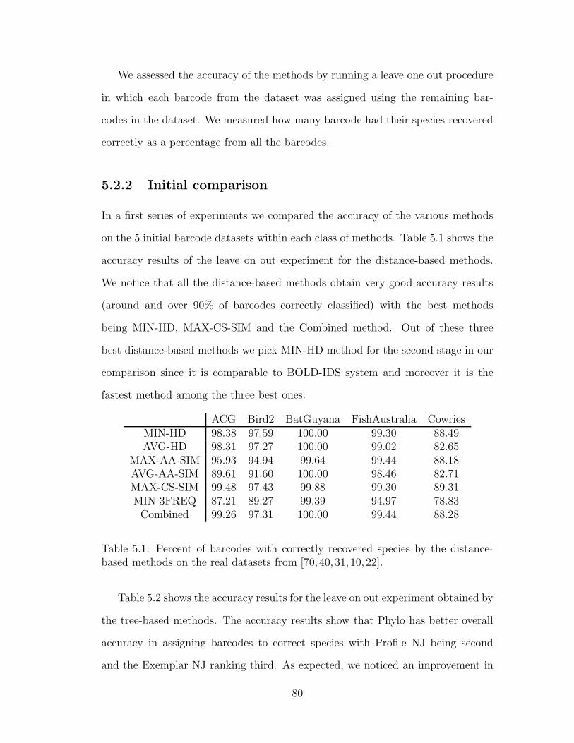
We assessed the accuracy of the methods by running a leave one out procedure
in which each barcode from the dataset was assigned using the remaining bar-
codes in the dataset. We measured how many barcode had their species recovered
correctly as a percentage from all the barcodes.
5.2.2 Initial comparison
In a first series of experiments we compared the accuracy of the various methods
on the 5 initial barcode datasets within each class of methods. Table 5.1 shows the
accuracy results of the leave on out experiment for the distance-based methods.
We notice that all the distance-based methods obtain very good accuracy results
(around and over 90% of barcodes correctly classified) with the best methods
being MIN-HD, MAX-CS-SIM and the Combined method. Out of these three
best distance-based methods we pick MIN-HD method for the second stage in our
comparison since it is comparable to BOLD-IDS system and moreover it is the
fastest method among the three best ones.
ACG Bird2 BatGuyana FishAustralia CowriesMIN-HD 98.38 97.59 100.00 99.30 88.49AVG-HD 98.31 97.27 100.00 99.02 82.65
MAX-AA-SIM 95.93 94.94 99.64 99.44 88.18AVG-AA-SIM 89.61 91.60 100.00 98.46 82.71MAX-CS-SIM 99.48 97.43 99.88 99.30 89.31MIN-3FREQ 87.21 89.27 99.39 94.97 78.83Combined 99.26 97.31 100.00 99.44 88.28
Table 5.1: Percent of barcodes with correctly recovered species by the distance-based methods on the real datasets from [70, 40, 31, 10, 22].
Table 5.2 shows the accuracy results for the leave on out experiment obtained by
the tree-based methods. The accuracy results show that Phylo has better overall
accuracy in assigning barcodes to correct species with Profile NJ being second
and the Exemplar NJ ranking third. As expected, we noticed an improvement in
80
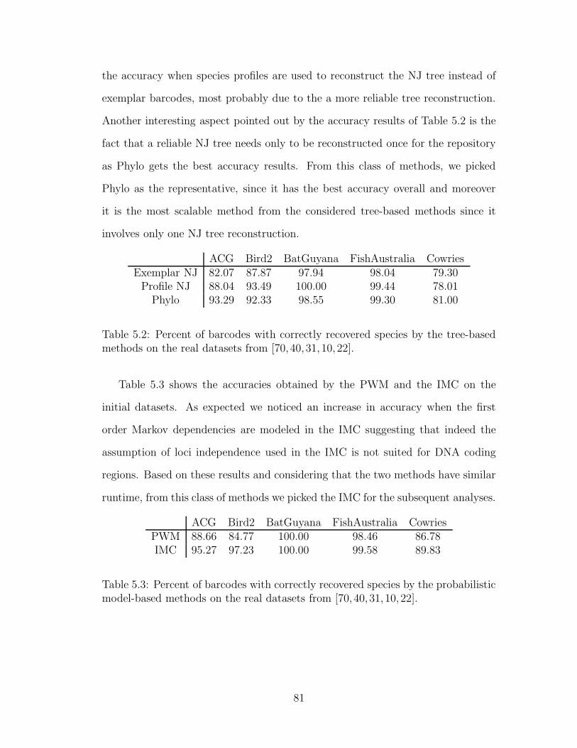
the accuracy when species profiles are used to reconstruct the NJ tree instead of
exemplar barcodes, most probably due to the a more reliable tree reconstruction.
Another interesting aspect pointed out by the accuracy results of Table 5.2 is the
fact that a reliable NJ tree needs only to be reconstructed once for the repository
as Phylo gets the best accuracy results. From this class of methods, we picked
Phylo as the representative, since it has the best accuracy overall and moreover
it is the most scalable method from the considered tree-based methods since it
involves only one NJ tree reconstruction.
ACG Bird2 BatGuyana FishAustralia CowriesExemplar NJ 82.07 87.87 97.94 98.04 79.30
Profile NJ 88.04 93.49 100.00 99.44 78.01Phylo 93.29 92.33 98.55 99.30 81.00
Table 5.2: Percent of barcodes with correctly recovered species by the tree-basedmethods on the real datasets from [70, 40, 31, 10, 22].
Table 5.3 shows the accuracies obtained by the PWM and the IMC on the
initial datasets. As expected we noticed an increase in accuracy when the first
order Markov dependencies are modeled in the IMC suggesting that indeed the
assumption of loci independence used in the IMC is not suited for DNA coding
regions. Based on these results and considering that the two methods have similar
runtime, from this class of methods we picked the IMC for the subsequent analyses.
ACG Bird2 BatGuyana FishAustralia CowriesPWM 88.66 84.77 100.00 98.46 86.78IMC 95.27 97.23 100.00 99.58 89.83
Table 5.3: Percent of barcodes with correctly recovered species by the probabilisticmodel-based methods on the real datasets from [70, 40, 31, 10, 22].
81
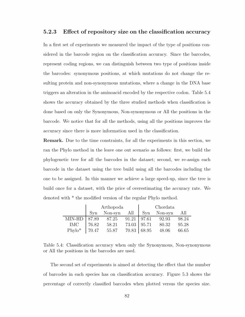
5.2.3 Effect of repository size on the classification accuracy
In a first set of experiments we measured the impact of the type of positions con-
sidered in the barcode region on the classification accuracy. Since the barcodes,
represent coding regions, we can distinguish between two type of positions inside
the barcodes: synonymous positions, at which mutations do not change the re-
sulting protein and non-synonymous mutations, where a change in the DNA base
triggers an alteration in the aminoacid encoded by the respective codon. Table 5.4
shows the accuracy obtained by the three studied methods when classification is
done based on only the Synonymous, Non-synonymous or All the positions in the
barcode. We notice that for all the methods, using all the positions improves the
accuracy since there is more information used in the classification.
Remark. Due to the time constraints, for all the experiments in this section, we
ran the Phylo method in the leave one out scenario as follows: first, we build the
phylogenetic tree for all the barcodes in the dataset; second, we re-assign each
barcode in the dataset using the tree build using all the barcodes including the
one to be assigned. In this manner we achieve a large speed-up, since the tree is
build once for a dataset, with the price of overestimating the accuracy rate. We
denoted with * the modified version of the regular Phylo method.
Arthopoda ChordataSyn Non-syn All Syn Non-syn All
MIN-HD 87.89 87.25 91.21 97.61 92.93 98.24IMC 76.82 58.21 73.03 95.71 80.32 95.28
Phylo* 70.47 55.87 70.83 68.95 48.06 66.65
Table 5.4: Classification accuracy when only the Synonymous, Non-synonymousor All the positions in the barcodes are used.
The second set of experiments is aimed at detecting the effect that the number
of barcodes in each species has on classification accuracy. Figure 5.3 shows the
percentage of correctly classified barcodes when plotted versus the species size.
82
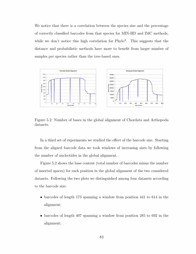
We notice that there is a correlation between the species size and the percentage
of correctly classified barcodes from that species for MIN-HD and IMC methods,
while we don’t notice this high correlation for Phylo*. This suggests that the
distance and probabilistic methods have more to benefit from larger number of
samples per species rather than the tree-based ones.
Chordata Global Alignment
0
2000
4000
6000
8000
10000
12000
14000
16000
18000
1 101 201 301 401 501 601 701 801 901
Base Position
Nu
mb
er
of
ba
se
s
Arthopoda Global Alignment
0
5000
10000
15000
20000
25000
30000
35000
40000
1 101 201 301 401 501 601 701 801 901
Base Position
Nu
mb
er
of
ba
se
s
Figure 5.2: Number of bases in the global alignment of Chordata and Arthopodadatasets.
In a third set of experiments we studied the effect of the barcode size. Starting
from the aligned barcode data we took windows of increasing sizes by following
the number of nucleotides in the global alignment.
Figure 5.2 shows the base content (total number of barcodes minus the number
of inserted spaces) for each position in the global alignment of the two considered
datasets. Following the two plots we distinguished among four datasets according
to the barcode size:
• barcodes of length 173 spanning a window from position 441 to 614 in the
alignment;
• barcodes of length 407 spanning a window from position 285 to 692 in the
alignment;
83
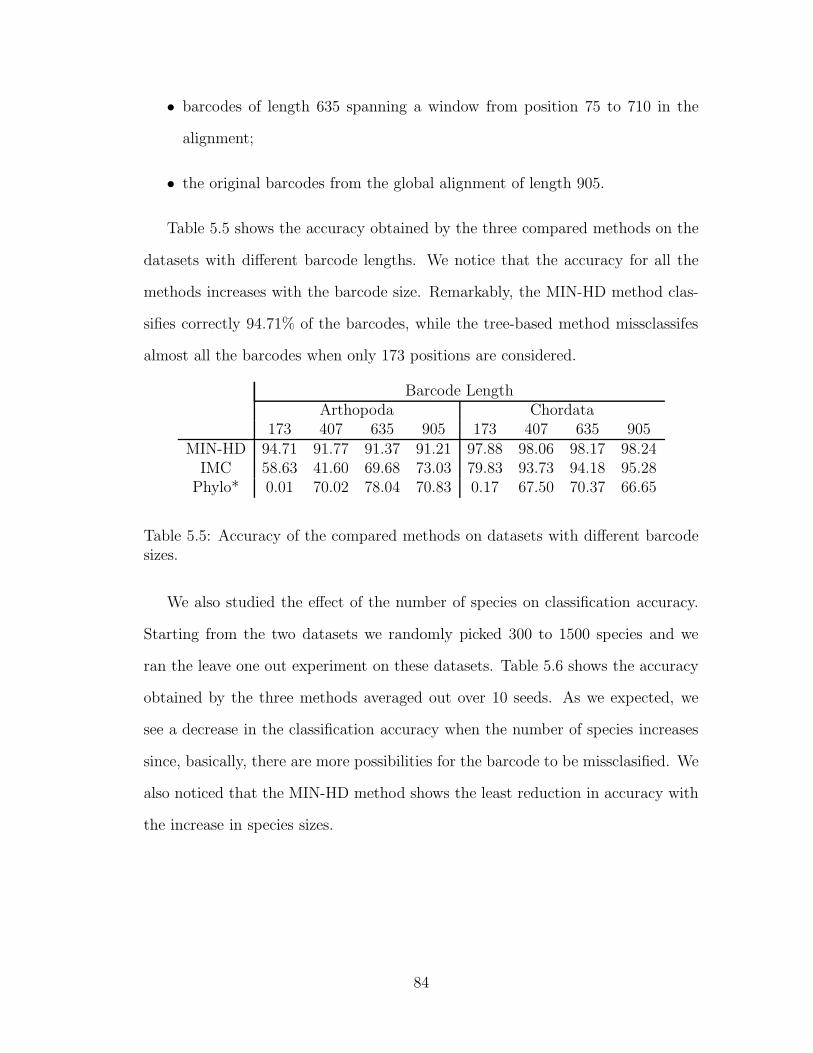
• barcodes of length 635 spanning a window from position 75 to 710 in the
alignment;
• the original barcodes from the global alignment of length 905.
Table 5.5 shows the accuracy obtained by the three compared methods on the
datasets with different barcode lengths. We notice that the accuracy for all the
methods increases with the barcode size. Remarkably, the MIN-HD method clas-
sifies correctly 94.71% of the barcodes, while the tree-based method missclassifes
almost all the barcodes when only 173 positions are considered.
Barcode LengthArthopoda Chordata
173 407 635 905 173 407 635 905MIN-HD 94.71 91.77 91.37 91.21 97.88 98.06 98.17 98.24
IMC 58.63 41.60 69.68 73.03 79.83 93.73 94.18 95.28Phylo* 0.01 70.02 78.04 70.83 0.17 67.50 70.37 66.65
Table 5.5: Accuracy of the compared methods on datasets with different barcodesizes.
We also studied the effect of the number of species on classification accuracy.
Starting from the two datasets we randomly picked 300 to 1500 species and we
ran the leave one out experiment on these datasets. Table 5.6 shows the accuracy
obtained by the three methods averaged out over 10 seeds. As we expected, we
see a decrease in the classification accuracy when the number of species increases
since, basically, there are more possibilities for the barcode to be missclasified. We
also noticed that the MIN-HD method shows the least reduction in accuracy with
the increase in species sizes.
84
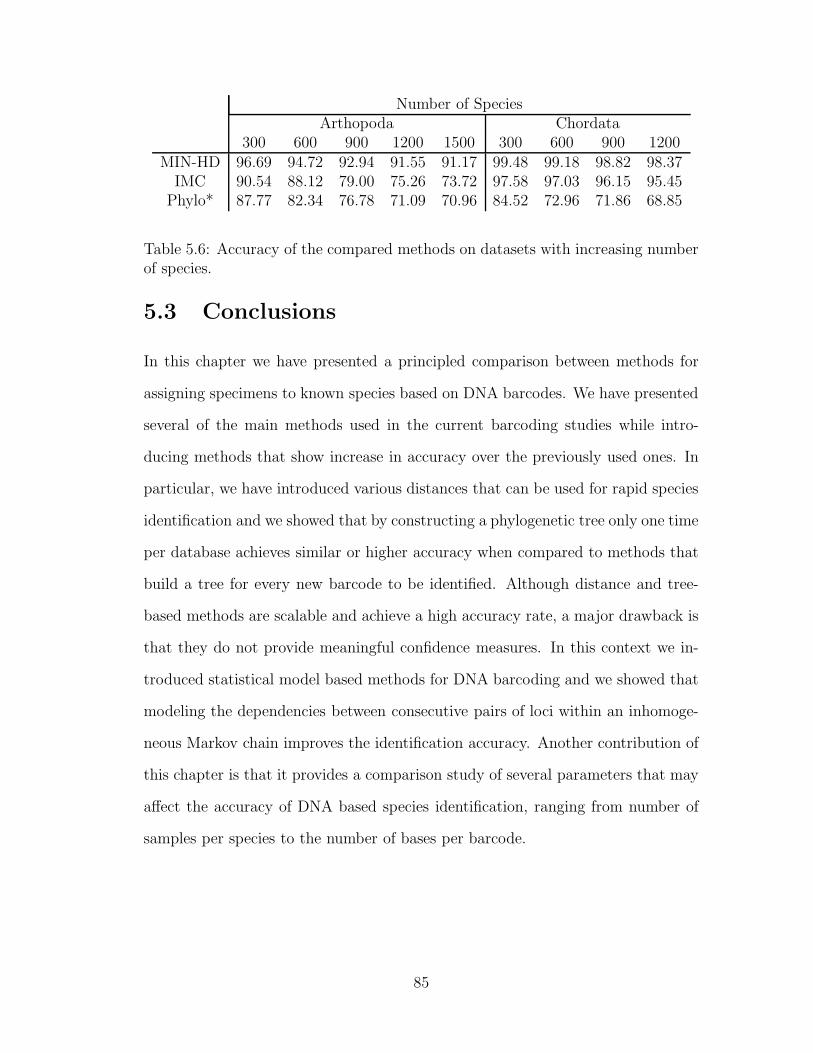
Number of SpeciesArthopoda Chordata
300 600 900 1200 1500 300 600 900 1200MIN-HD 96.69 94.72 92.94 91.55 91.17 99.48 99.18 98.82 98.37
IMC 90.54 88.12 79.00 75.26 73.72 97.58 97.03 96.15 95.45Phylo* 87.77 82.34 76.78 71.09 70.96 84.52 72.96 71.86 68.85
Table 5.6: Accuracy of the compared methods on datasets with increasing numberof species.
5.3 Conclusions
In this chapter we have presented a principled comparison between methods for
assigning specimens to known species based on DNA barcodes. We have presented
several of the main methods used in the current barcoding studies while intro-
ducing methods that show increase in accuracy over the previously used ones. In
particular, we have introduced various distances that can be used for rapid species
identification and we showed that by constructing a phylogenetic tree only one time
per database achieves similar or higher accuracy when compared to methods that
build a tree for every new barcode to be identified. Although distance and tree-
based methods are scalable and achieve a high accuracy rate, a major drawback is
that they do not provide meaningful confidence measures. In this context we in-
troduced statistical model based methods for DNA barcoding and we showed that
modeling the dependencies between consecutive pairs of loci within an inhomoge-
neous Markov chain improves the identification accuracy. Another contribution of
this chapter is that it provides a comparison study of several parameters that may
affect the accuracy of DNA based species identification, ranging from number of
samples per species to the number of bases per barcode.
85
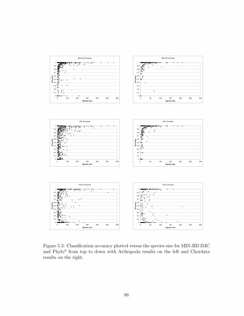
MIN-HD Arthopoda
0
0.1
0.2
0.3
0.4
0.5
0.6
0.7
0.8
0.9
1
0 100 200 300 400 500 600
Species size
Ac
cu
rac
y
MIN-HD Chordata
0
0.1
0.2
0.3
0.4
0.5
0.6
0.7
0.8
0.9
1
0 50 100 150 200 250 300
Species size
Accu
racy
IMC Arthopoda
0
0.1
0.2
0.3
0.4
0.5
0.6
0.7
0.8
0.9
1
0 100 200 300 400 500 600
Species size
Ac
cu
rac
y
IMC Chordata
0
0.1
0.2
0.3
0.4
0.5
0.6
0.7
0.8
0.9
1
0 50 100 150 200 250 300
Species size
Accu
racy
Phylo Arthopoda
0
0.1
0.2
0.3
0.4
0.5
0.6
0.7
0.8
0.9
1
0 100 200 300 400 500 600
Species size
Acc
ura
cy
Phylo Chordata
0
0.1
0.2
0.3
0.4
0.5
0.6
0.7
0.8
0.9
1
0 50 100 150 200 250 300
Species size
Acc
ura
cy
Figure 5.3: Classification accuracy plotted versus the species size for MIN-HD IMCand Phylo* from top to down with Arthopoda results on the left and Chordataresults on the right.
86
Chapter 6
Conclusions
The need for highly scalable methods is expected to increase in the future with
the need of handling the large amount of data to be produced by next gener-
ation of genome-wide association studies. High-end genotyping platforms from
Affymetrix an Illumina already allow typing over half a million SNP genotypes per
experiment, with one million SNP genotypes per experiment expected in the very
near future. Furthermore, due to decreasing genotyping costs, current association
studies are already comprising thousands of typed individuals [38]. In this the-
sis we have introduced highly-scalable algorithms for several computational and
statistical problems that arise in the context of current genomic studies.
In the first chapter, we introduced ENT, a highly scalable algorithm for infer-
ring haplotypes from the genotype data. ENT has been implemented as an open
source software package which is publicly available, together with a web server, at
http://dna.engr.uconn.edu/~software/ent/. A unique feature of our package
is that it can handle related genotypes coming from complex pedigrees, which can
lead to significant improvements in phasing accuracy over methods that do not
take into account pedigree information. We have conducted an extensive compar-
ison of our method with the currently state of the art methods for phasing on
87
simulated and real datasets showing that ENT gains scalability over the available
methods while maintaining an accuracy close to the best methods for phasing.
In chapter 2 we presented an approach towards modeling the Linkage Disequi-
librium variation observed in the haplotypes of a population through the use of
a Hidden Markov Model (HMM) of haplotype diversity. Our proposed HMM has
a structure similar to that of models recently used for other haplotype analysis
problems including genotype phasing, testing for disease association, and impu-
tation [56, 39, 51, 32, 57]. Intuitively, the HMM represents a number of K founder
haplotypes along high-probability “horizontal” paths of states, while capturing
observed recombination between pairs of founder haplotypes via probabilities of
“non-horizontal” transitions. After describing the model we showed that com-
puting the maximum phasing probability when the haplotype frequencies are rep-
resented through the HMM problem is hard solving an important open problem
in [51]. We introduce next several alternate likelihood functions that can be used
in the context of genotype phasing and we show that the phasing obtained by sev-
eral methods including ENT can be further improved by a local 1-OPT tweaking
procedure inside the HMM within the maximum likelihood approach. In Chap-
ter 4 we show that the HMM we presented can be used for of other problems in
the context of genomic studies, such as imputation and error detection. We show
here how our model can be used as a computational basis for efficiently computing
probabilities of observing genotypes in samples at typed or untyped markers, prob-
abilities that can be used to either detect or correct errors in the genotype calling
or to impute missing genotypes in conjunction with haplotypes from catalogues of
variation such as HapMap.
In Chapter 5 we introduced new methods for assigning samples to categorizes
species from a repository based on short genomic DNA sequences, called DNA bar-
codes. Within this context we apply the HMM of haplotype diversity to represent
88

the variability observed in the DNA barcodes of the same species by simplifying
it into an Inhomogeneous Markov Chain model (IMC). We presented a compari-
son between the methods already proposed for DNA barcoding and our proposed
methods focusing on the parameters required from the repository (number of bar-
codes per species, size of the barcode region, etc) in order to make a reliable species
identification.
89
Bibliography
[1] H. Ackerman, S. Usen, R. Mott, A. Richardson, F. Sisay-Joof, P. Katundu,
T.Taylor, R. Ward, M. Molyneux, M. Pinder, and D. P. Kwiatkowski. Haplo-
typic analysis of the tnf locus by association efficiency and entropy. Genome
Biology, 4:R24.1–R24.13, 2003.
[2] S. Angelov, B. Harb, S. Kannan, S. Khanna, and J. Kim. Efficient enumer-
ation of phylogenetically informative substrings. Lecture Notes in Computer
Science, 3909:248–264, 2006.
[3] L.E. Baum, T. Petrie, G. Soules, and N. Weiss. A maximization technique
occurring in the statistical analysis of probabilistic functions of Markov chains.
Annals of Mathematical Statistics, 41:164–171, 1970.
[4] T. Becker, R. Valentonyte, P. Croucher, K. Strauch, S. Schreiber, J. Hampe,
and M. Knapp. Identification of probable genotyping errors by consideration
of haplotypes. European Journal of Human Genetics, 14:450–458, 2006.
[5] D. Branza, J. He, W. Mao, and A. Zelikovsky. Phasing and missing data
recovery in family trios. Lecture Notes in Computer Science, 3515:1011–1019,
2005.
[6] D. Branza and A. Zelikovsky. 2SNP: scalable phasing based on 2-SNP haplo-
types. Bioinformatics, 22(3):371–373, 2006.
90
[7] D.G. Brown and I.M. Harrower. A new integer programming formulation for
the pure parsimony problem in haplotype analysis. In I. Jonassen and J. Kim,
editors, Algorithms in Bioinformatics, 4th International Workshop (WABI),
volume 3240 of Lecture Notes in Bioinformatics, pages 254–265, 2004.
[8] B.L. Browning and S.R. Browning. Efficient multilocus association mapping
for whole genome association studies using localized haplotype clustering. Ge-
netics Epidemiology, 31:365–375, 2007.
[9] S.R. Browning and B.L. Browning. Rapid and accurate haplotype phasing and
missing data inference for whole genome association studies using localized
haplotype clustering. American Journal of Human Genetics, 81:1084–1097,
2007.
[10] E.L. Clare, B.K. Lim, M.D. Engstrom, J.L. Eger, and P.D.N. Hebert. Dna bar-
coding of neotropical bats: species identification and discovery within guyana.
Molecular Ecology Notes, 7:184–190, 2007.
[11] The International HapMap Consortium. The international hapmap project.
Nature, 426:789–796, 2003.
[12] The International HapMap Consortium. A haplotype map of the human
genome. Nature, 437:1299–1320, 2005.
[13] The International HapMap Consortium. A second generation human haplo-
type map of over 3.1 million snps. Nature, 449:851–861, 2007.
[14] The Wellcome Trust Consortium. Genome-wide association study of 14,000
cases of seven common diseases and 3,000 shared controls. Nature, 447:661–
678, 2007.
91
[15] M.J. Daly, J.D. Rioux, S.F. Schaffner, T.J. Hudson, and E.S. Lander. High-
resolution haplotype structure in the human genome. Nature Genetics,
29(2):229–232, 2001.
[16] R. Durbin, S. Eddy, A. Krogh, and G. Mitchinson. Biological sequence analy-
sis: Probabilistic Models of Proteins and Nucleic Acids. Cambridge University
Press, Cambridge UK, 1998.
[17] T. Ekrem, E. Willassen, and E. Stur. A comprehensive dna library is essential
for identification with dna barcodes. Molecular Phylogenetics and Evolution,
43:530–542, 2007.
[18] E. Eskin, E. Halperin, and R. Sharan. Optimally phasing long genomic regions
using local haplotype predictions. In Second RECOMB Satellite Workshop on
Computational Methods for SNPs and Haplotypes, pages 13–16, 2004.
[19] A. Gusev, I.I. Mandoiu, and B. Pasaniuc. Highly scalable genotype phasing by
entropy minimization. IEEE/ACM Transactions on Computational Biology
and Bioinformatics (to appear), 2007.
[20] D. Gusfield. Haplotyping by pure parsimony. In Proc. 14th Annual Symp. on
Combinatorial Pattern Matching (CPM), pages 144–155, 2003.
[21] D. Gusfield. An overview of combinatorial methods for haplotype inference.
In Proc. DIMACS/RECOMB Satellite Workshop on Computational Methods
for SNPs and Haplotype Inference, pages 9–25, 2004.
[22] M. Hajibabaei, D.H. Janzen, J.M. Burns, W. Hallwachs, and P.D.N. Hebert.
Dna barcodes distinguish species of tropical lepidoptera. PNAS, 103:968–971,
2006.
92
[23] B.V. Halldorsson, V. Bafna, N. Edwards, R. Lippert, S. Yooseph, and S. Is-
trail. A survey of computational methods for determining haplotypes. In
Proc. DIMACS/RECOMB Satellite Workshop on Computational Methods for
SNPs and Haplotype Inference, pages 26–47, 2004.
[24] E. Halperin and E. Eskin. Haplotype reconstruction from genotype data using
imperfect phylogeny. Bioinformatics, 20:1842–1849, 2004.
[25] E. Halperin and R.M. Karp. The minimum-entropy set cover problem. In Proc.
Annual International Colloquium on Automata, Languages and Programming
(ICALP), 2004.
[26] J. Hastad. Clique is hard to approximate within n1−ε. Acta Mathematica,
182:105–142, 1999.
[27] P. Hebert, S. Ratnasingham, and JR. deWaard. Barcoding animal life: cy-
tochrome c oxidase subunit 1 divergences among closely related species. In
Proc. Royal Society London, 2003.
[28] P.D.N. Hebert, A. Cywinska, and S.L. Balland J.R. deWaard. Biological iden-
tifications through dna barcodes. Phil. Trans. R. Soc. B: Biological Sciences,
270:313–321, 2003.
[29] S. Henikoff and JG. Henikoff. Amino acid substitution matrices from protein
blocks. PNAS, 88.
[30] J. Kennedy, I.I. Mandoiu, and B. Pasaniuc. Genotype error detection using
hidden Markov models of haplotype diversity. In Proc. 7th Workshop on
Algorithms in Bioinformatics, Lecture Notes in Computer Science, pages 73–
84, 2007.
93
[31] K.C.R. Kerr, M.Y. Stoeckle, C.J. Dove, L.A. Weigt, C.M. Frances, and P.D.N.
Hebert. Comprehensive dna barcode coverage of north american birds. Molec-
ular Ecology Notes (doi:10.1111/j.1471-8286.2006.01670.x), 2007.
[32] G. Kimmel and R. Shamir. A block-free hidden Markov model for genotypes
and its application to disease association. Journal of Computational Biology,
12:1243–1260, 2005.
[33] J Kuntsi, BM Neale, W Chen, SV Faraone, and P. Asherson. The IMAGE
project: methodological issues for the molecular genetic analysis of ADHD.
Genome Res., 2:27, 2006.
[34] G. Lancia, M.C. Pinotti, and R. Rizzi. Haplotyping populations by pure
parsimony: Complexity of exact and approximation algorithms. INFORMS
Journal on Computing, 16:348–359, 2004.
[35] Y. Li and G. R. Abecasis. Mach 1.0: Rapid haplotype reconstruction and
missing genotype inference. American Journal of Human Genetics, 79:2290,
2006.
[36] S. Lin, A. Chakravarti, and D.J. Cutler. Haplotype and Missing Data Infer-
ence in Nuclear Families. Genome Research, 14(8):1624–1632, 2004.
[37] R.B. Lyngso and C.N.S. Pedersen. The consensus string problem and the com-
plexity of comparing hidden markov models. Journal of Computer Systems
Science, 65(3):545–569, 2002.
[38] J. Marchini, D. Cutler, N. Patterson, M. Stephens, E. Eskin, E. Halperin,
S. Lin, Z.S. Qin, H.M. Munro, G.R. Abecasis, P. Donnelly, and International
HapMap Consortium. A comparison of phasing algorithms for trios and un-
related individuals. American Journal of Human Genetics, 78:437–450, 2006.
94
[39] J. Marchini, B. Howie, S. Myers, G. McVean, and P. Donnelly. A new multi-
point method for genome-wide association studies by imputation of genotypes.
Nature Genetics, 39:906–913, 2007.
[40] C.P. Meyer and G. Paulay. Dna barcoding: Error rates based on comprehen-
sive sampling. PLoS Biology, 3, 2005.
[41] S.E. Miller. Dna barcoding and the renaissance of taxonomy. PNAS, 104:4775–
4776, 2007.
[42] I.I. Mandoiu and B. Pasaniuc. Haplotype inference by entropy minimiza-
tion. In 9th Annual International Conference on Research in Computational
Molecular Biology (RECOMB) Poster Book, pages 221–222, 2005.
[43] N. Nagarajan, N. Jones, and U. Keich. Computing the p-value of the in-
formation content from an alignment of multiple sequences. Bioinformatics,
21:311–318, 2005.
[44] R. Nielsen and M. Matz. Statistical approaches for dna barcoding. Syst Biol.,
55:162–169, 2006.
[45] T. Niu. Algorithms for inferring haplotypes. Genetics Epidemiology, 27:334–
347, 2004.
[46] S. H. Orzack, D. Gusfield, J. Olson, S. Nesbitt, L. Subrahmanyan, and
V. P. Stanton Jr. Analysis and Exploration of the Use of Rule-Based Al-
gorithms and Consensus Methods for the Inferral of Haplotypes. Genetics,
165(2):915–928, 2003.
[47] B. Pasaniuc and I.I. Mandoiu. Highly scalable genotype phasing by entropy
minimization. In Proc. 28th Annual International Conference of the IEEE
Engineering in Medicine and Biology Society, pages 3482–3486, 2006.
95
[48] F. Pompanon, A. Bonin, E. Bellemain, and P. Taberlet. Genotyping errors:
causes, consequences and solutions. Nature Review Genetics, 6:847–859, 2005.
[49] Z.S. Qin, T. Niu, and J.S. Liu. Partition-ligation – expectation-maximization
algorithm for haplotype inference with single-nucleotide polymorphisms.
Americal Journal of Human Genetics, 71:1242–1247, 2002.
[50] S. Rahmann. Dynamic programming algorithms for two statistical problems
in computational biology. Proceedings of the 3rd Workshop of Algorithms in
Bioinformatics (WABI), 2812:151–164, 2003.
[51] P. Rastas, M. Koivisto, H. Mannila, and E. Ukkonen. Phasing genotypes
using a hidden Markov model. In Bioinformatics Algorithms: Techniques and
Applications, pages 355–373. Wiley, 2008, preliminary version in Proc. WABI
2005.
[52] S. Ratnasingham and P.D.N. Hebert. Bold: The barcode of life data system
(http://www.barcodinglife.org). Molecular Ecology Notes, 7:355–364, 2007.
[53] N. Saitou and M. Nei. The neighbor-joining method: a new method for
reconstructing phylogenetic trees. Molecular Biology and Evolution, 4:406–
425, 1987.
[54] R.M. Salem, J. Wessel, and N.J. Schork. A comprehensive literature review of
haplotyping software and methods for use with unrelated individuals. Human
Genomics, 2:39–66, 2005.
[55] V. Savolainen, R.S. Cowan, A.P. Vogler, G.K. Roderick, and R. Lane. Towards
writing the encyclopaedia of life: an introduction to dna barcoding. Phil.
Trans. R. Soc. B: Biological Sciences, 360:1805–1811, 2005.
96
[56] P. Scheet and M. Stephens. A fast and flexible statistical model for large-
scale population genotype data: applications to inferring missing genotypes
and haplotypic phase. American Journal of Human Genetics, 78:629–644,
2006.
[57] R. Schwartz. Haplotype motifs: An algorithmic approach to locating evo-
lutionarily conserved patterns in haploid sequences. In Proc. CSB, pages
306–315, 2003.
[58] R. Schwartz. Algorithms for association study design using a generalized
model of haplotype conservation. In Proc. CSB, pages 90–97, 2004.
[59] D. Steinke, M. Vences, W. Salzburger, and A. Meyer. Taxi: a software tool
for dna barcoding using distance methods. Phil. Trans. R. Soc. B: Biological
Sciences, 360:1975–1980, 2005.
[60] M. Stephens and P. Donnelly. A comparison of bayesian methods for haplotype
reconstruction from population genotype data. American Journal of Human
Genetics, 73:1162–1169, 2003.
[61] M. Stephens and P. Scheet. Accounting for decay of linkage disequilibrium
in haplotype inference and missing-data imputation. American Journal of
Human Genetics, 76:449–462, 2005.
[62] M. Stephens, N. J. Smith, and Peter Donnelly. A new statistical method for
haplotype reconstruction from population data. American Journal of Human
Genetics, 68:978–989, 2001.
[63] A. Stolcke and S. M. Omohundro. Hidden markov model induction by bayesian
model merging. Advances in Neural Information Processing Systems 5, pages
11–18, 1992.
97
[64] A. Sundquist, E. Fratkin, C.B. Do, and S. Batzoglou. Effect of genetic
divergence in identifying ancestral origin using hapaa. Genome Research,
18(4):676–682, 2008.
[65] http://www.affymetrix.com/products/arrays/specific/500k.affx.
[66] http://www.barcoding.si.edu.
[67] http://www.fnih.org/GAIN2/home_new.shtml.
[68] A.J. Viterbi. Error bounds for convolutional codes and an asymptotically
optimum decoding algorithm. IEEE Transactions on Information Theory,
13:260–269, 1967.
[69] L. Wang and Y. Xu. Haplotype inference by maximum parsimony. Bioinfor-
matics, 19:1773–1780, 2003.
[70] R.D. Ward, T.S. Zemlak, B.H. Innes, P.R. Last, and P.D.N. Hebert. Dna
barcoding australia’s fish species. Phil. Trans. R. Soc. B: Biological Sci-
ences(doi:10.1098/rstb.2005.1716), 2005.
[71] X. Wen and D. L. Nicolae. Association studies for untyped markers with tuna.
Bioinformatics, 24:435–437, 2008.
[72] J. Xiao, L. Liu, L. Xia, and T. Jiang. Fast elimination of redundant lin-
ear equations and reconstruction of recombination-free mendelian inheritance
on a pedigree. In Accepted by ACM-SIAM Symposium on Discrete Algo-
rithms(SODA’2007), 2007.
[73] J. Zhang, B. Jiang, M. Li, J. Tromp, X.Zhang, and M.Q. Zhang. Computing
exact p-values for dna motifs. Bioinformatics, 23:531–537, 2007.
98