Asphalt Solar Collector and Borehole Storage Design study for a small residential building area

Master’s Thesis within Sustainable Energy Systems and Structural Engineering & Building Performance Design

SIEBERT Nicolas ZACHARAKIS Eleftherios Department of Energy and Environment Division of Building Services Engineering CHALMERS UNIVERSITY OF TECHNOLOGY Göteborg, Sweden 2010 Report No. E2010:11

MASTER’S THESIS

Asphalt Solar Collector and Borehole Storage Design study for a small residential building area

Master’s Thesis within Sustainable Energy Systems and Structural Engineering & Building Performance Design

SUPERVISOR

Kristine Ek

EXAMINER

Jan-Olof Dalenbäck

Department of Energy and Environment Division of Building Services Engineering

CHALMERS UNIVERSITY OF TECHNOLOGY

Göteborg, Sweden 2010

Asphalt Solar Collector and Borehole Storage Design study for a small residential building area Master’s Thesis in Sustainable Energy Systems and Structural Engineering & Building Performance Design

NICOLAS SIEBERT

ELEFTHERIOS ZACHARAKIS

© SIEBERT & ZACHARAKIS, 2010 Report No. E2010:11 Department of Energy and Environment Division of Building Services Engineering Chalmers University of Technology SE-412 96 Göteborg Sweden Telephone: + 46 (0)31-772 1000 Chalmers Reproservice Göteborg, Sweden 2010

I

Preface

This thesis represents the final part of the Master’s Programme in Sustainable Energy System along as in Structural Engineering and Building Performance Design at Chalmers University of Technology in Gothenburg, Sweden. More specifically, this project is a study case of a new sustainable energy system that tries to use the solar energy as green energy for heating demands of buildings with the use of asphalt pavements. This topic has been already an object of research in the recent last years by academic research groups and private companies, which have been trying to apply these researches in practice developing methodologies.

The study of this project has been prepared on behalf of NCC AB at Gothenburg and financed by Svenska Byggbranschens Utvecklingsfond (SBUF). For the reasons above, NCC AB and especially NCC Teknik department have been interested in the investigation of this technological innovation and the possibility of its application on the Swedish context. In that case, a new housing project in Fågelsten has been suggested for the application of an asphalt solar collector in the parking lot area. The final task lies on whether this system is competitive to the district heating that is the common heating method in Sweden. The project has been conducted from February to June 2010.

During the research and the preparation of this project a lot of people have contributed with their support for reaching our final goal. We would like to thank everyone in general and especially our families and our friends for their support, our examiner at Chalmers Jan – Olof Dalenbäck for his guidance and his advice on an academic level, Saqib Javed from the Sustainable Energy Department for his assistance on the fields of ground source heat pump design and Kristine Ek from NCC Teknik who provided us with information for the project in Fågelsten. Finally, we would like to thank each other for having a great cooperation and learning from each other in terms of knowledge, experience and cultural diversity.

Göteborg June 2010

Nicolas Siebert

Eleftherios Zacharkis

II

III

Asphalt Solar Collector and Borehole Storage Design study for a small residential building area Master’s Thesis in Sustainable Energy Systems and Structural Engineering & Building Performance Design SIEBERT & ZACHARAKIS Department of Energy and Environment Division of Building Services Engineering Chalmers University of Technology

Abstract

In order to use the solar energy for heating purposes a transfer into another form is required, with solar thermal collectors being the most common technique for domestic water heating. Taking into consideration the annual global radiation distribution and the land’s value for installing solar farms the idea of using the asphalt surfaces which consist of roads, pavements and parking lots, as a means of energy transfer into usable heat is worth while investigating.

This study is based on the interest of NCC, a Swedish building contractor, to investigate the possibilities to utilize asphalt areas as solar collectors. In the Swedish context and climate conditions, the main task was to investigate the application of an asphalt solar collector for heat capture and a ground source heat pump with borehole storage with the intention of using that heat for domestic hot water and heating demands in Fågelsten, a newly planned residential building area. The performance of the system is being examined from an energy and cost point of view along with the environmental impact. This performance is compared to the common used case of district heating and standard ground source heat pump in Sweden.

The system design has been conducted using the numerical modeling software COMSOL Multiphysics for the asphalt collector, while ground source heat pump and the borehole storage system were managed by Earth Energy Designer 3 (EED3). A global design of the system is proposed so as to cover the energy demands, followed by a basic economical and environmental analysis. Conclusions have been written concerning the global performance and applicability of that system.

Key words:

Asphalt solar collector, ground source heat pump, borehole storage, heat transfer, sustainable energy.

IV

V

Contents

PREFACE I 

ABSTRACT III 

CONTENTS V 

1  INTRODUCTION 1 

1.1  Background 1 

1.2  Objectives 2 

1.3  Method 2 

1.4  Limitations 4 

2  PREVIOUS STUDIES AND APPLICATIONS 5 

2.1  Background and previous literature review 5 

2.2  SERSO Project 7 

2.3  TRL Report 10 

2.4  Worcester Polytechnic Institute Research 13 

2.5  Road Energy Systems 16 

2.6  Studies comparison 20 

3  SOLAR ENERGY AND TEMPERATURE 21 

3.1  Solar energy potentials 21 

3.2  Solar irradiation 22 

3.3  Temperature profiles 24 

4  SYSTEMS AND COMPONENTS 27 

4.1  Solar collectors 27 

4.2  Ground source heat pumps 28 

4.3  Thermal storage systems 32 

4.4  Combination of ground source heat pumps and solar collectors 33 

5  BUILDING ENERGY DEMANDS 35 

5.1  Domestic energy consumption principles 35 

5.2  Fågelsten residential area energy demands 36 

VI

6  ASPHALT SOLAR COLLECTOR 39 

6.1  Theory 39 

6.1.1 Analytical approach 39 

6.1.2 Energy balance of an asphalt pavement 43 

6.1.3 Finite elements analysis of the energy balance on the asphalt pavements 45 

6.2  Modeling 47 

6.2.1 The asphalt pavement model 47 

6.2.2 The geometry of the base case model 49 

6.2.3 Meshing of the base case model 49 

6.2.4 Post-processing of the base case model 50 

6.2.5 The asphalt pavement mixture 51 

6.2.6 The asphalt surface temperature 52 

6.2.7 The water – ethanol mixture in the piping system 54 

6.2.8 Parameters influence investigation 55 

6.2.9 Sensitivity analysis of the parameters 75 

7  BOREHOLE STORAGE 85 

7.1 Theory 85 

7.1.1 The most typical models 85 

7.1.2 The typical programs 86 

7.2  EED overview 87 

7.3  Modeling 88 

7.4 Design data 89 

8  GLOBAL SYSTEM DESIGN 99 

9  ECONOMICAL ESTIMATION 111 

10  ENVIRONMENTAL IMPACT 119 

11  CONCLUSIONS AND DISCUSSION 123

REFERENCES 126 

LIST OF ANNEXES 130

1

1 INTRODUCTION

1.1 Background The human comfort and adaptation to every existing condition of any context

has been always the main reason for the investigation and research of new technologies which will assist the way of living and consequently to lead to further development. In order to cover principle surviving demands people have taken into advantage the natural resources they could use neglecting the possibility of the resources extinction in future terms and the effect of their use. The exploitation to a great extent of these resources has led to a critical point where there is an urgent need to reconsider the term of energy and focus to sustainable energy reasonability in order that the energy to meet the energy of the present without compromising the ability of future generations to meet their needs.

Currently, the energy sector deals with the fossil fuels depletion and greenhouse gas emissions. These issues are reinforced by the growing energy consumption worldwide. The energy sector has to put efforts in renewable energy as well as energy optimization measures. Renewable energy, such as wind power, solar (heat & power), geothermal (heat & power), can take the place of current primary energy supply sources or improvements can also be made in energy conversion, transportation and distribution. Primary energy sources are converted into heat, electricity or can be directly used for transportation purpose to supply energy to the industrial, residential and transportation sectors contributing to a sustainable management.

The heating of buildings represents the main part of the residential energy use. In Sweden, heating is mainly provided by district heating, electricity and bio-fuels. These systems have been optimized to work with the most possible efficient way in reference to the cost and the CO2 emissions. It seems though that there are greater potentials of succeeding the same results with less costs and emissions through the combination of the renewable and the conservation energy systems especially in cases of integrating these systems into existing ones.

There is a large theoretical potential to use solar energy to cover heat demands in buildings. The technical potential on northern latitudes is very much influenced by the possibilities to store heat from the summer period to the heating period. One way to cover the building heat demands is to use solar energy and seasonal storage in the ground, where the stored energy can be reused when needed. The capture of solar energy is commonly managed by some kind of solar collector mounted on roofs or on the ground. The capture of solar energy can also be achieved with the use of the asphalt surfaces, such as the pavements, the roads and the parking lots. The asphalt is a material with high heat capacity and acts as a thermal mass, indicating it can store large amounts of heat.

The idea of using asphalt solar collectors may be proved costly efficient in comparison to the traditional solar collector since the asphalt surfaces are already used and there is no need to be constructed or leased just for the case of energy capture. The energy system can be installed very easily since it is considered that the roads and the parking lots are usually resurfaced every 10-12 years time, so it can be done at that time. From the energy production point of view, the significantly larger areas of

2

the asphalt collectors can offset their expected lower efficiency and improve their efficiency in terms of an investment for the power produced per unit. Furthermore, the asphalt surfaces have the ability to continue producing energy even during the night when the solar collectors do not work.

The captured solar energy from the asphalt surfaces can be used for different applications, e.g. in combination with borehole heat storages, but requires in general the use of a pump to increase the temperature level for use in building heating systems. Additionally, this system can be a solution in other cases, such as for the road safety and maintenance by keeping the roads snow free during the winter time and decreasing the cost of regular resurfacing. Also, the heat island effect in the cities can be improved by the decrease of the asphalt surfaces temperatures contributing to a better climate.

1.2 Objectives The objectives of this master thesis were:

1. The investigation of the asphalt surfaces temperature profiles and how they are influenced by the air temperature, the solar irradiation and the wind through the year.

2. To model the temperature distribution on an asphalt parking lot with the use of basic heat transfer principles to decide the thermal properties of the asphalt.

3. To model the asphalt solar collector system and investigate the way the different parameters of each component are interacting for further optimization.

4. To design and model an asphalt solar collector system and estimate the potential extracted heat.

5. The interaction between the inserted heat, which was extracted from the solar asphalt system, and the ground source heat pump.

6. The economical estimation of the combined solar asphalt and ground source heat pump system.

7. The environmental analysis and impact.

8. The investigation of the possibility of using the system in a cost and environmental efficient way in comparison to the district heating system.

1.3 Method The methodology that has been used for the approach of this study has been based on four main stages. These stages are summed up in Table 1.3 and in each one of them further descriptions are given for the different approaches that were taken.

3

Table 1.3 The methodology stages and the description of each stage.

Methodology stages Description

1. Data collection • Climate data by NASA

• Asphalt data Trafikverket

2. Performance research • Asphalt solar collector by using COMSOL Multiphysics

• Ground source heat pump by using EED

3. Global system design • Matching of the two systems

• Global system design proposal

4. Evaluation • Energy demands

• Cost estimation

• Environmental impact

In the first stage, the collection of the climate and asphalt data from the area where Fågelsten is, should be gathered in order to be used in the following stages as input data. The climate data have been taken by NASA measurements and include the average monthly temperatures of the air and the earth temperature, the average wind speed, while the measured values of the asphalts surface for everyday and every hour during the year 2009 were provided by Trafikverket.

The second stage concerned the simulation of an asphalt collector and the investigation of its performance under different parameters options. The software COMSOL Multiphysics 3.5.a [1], provided by Chalmers University, and the General Heat Transfer Module [2] were used for simulating the asphalt collector. The outputs from that software were the developed temperatures in the asphalt collector. These outputs were used as indirect inputs in the software EED [3] for the design of the ground source heat pump. That means that a series of trials were made in EED runs so as to match the outputs from COMSOL with the outputs of EED in the way the need to cover the heat demands of the building.

During the third stage, the different trials in COMSOL in EED were compared and matched so as to meet the demands. The design of a global system was proposed including the design of an asphalt collector and a ground source heat pump that together could cooperate and supply the building with the amount of heat it needs.

In the fourth and last stage, the proposed global system was examined in regards of the cost and the environmental impact. The cost has been estimated in comparison to the base case of the district heating, while the environmental impact focused in the greenhouse gas emissions of the new system in comparison to the district heating and other producers.

4

1.4 Limitations The study has been done in collaboration with NCC, which has given a

specific case study to work with. The study is focused on a residential building project under construction in Lindome, Fågelsten, in the south of Göteborg. This project deals with a cluster of three multi-family dwellings and three storage rooms. The investigation of the use of an asphalt collector system for the parking lot area of these dwellings has been requested by NCC. Combined with a heat pump and a borehole seasonal storage system, this system will provide heat for domestic hot water generation and for building heating purpose. The residential Swedish context implies that cooling loads will not be needed in the study. This solar-assisted heat pump system has to be compared to the standard district heating system from energy, economical and environmental point of view.

As a consequence, the data used for simulation inputs or for different analysis are based on Swedish conditions. Some parameters have been estimated because of a lack of data or have kept constant because of their slight variation or a large computing time in the simulations. The major example is the choice of using steady-state simulations for the study of the asphalt collector. Due to the size of the system and the computing power, monthly steady state studies have been done. Monthly average data has been used, especially the air temperature input, for the non-time-dependent studies. Concerning the interseasonal storage in the ground, there was a need to make assumptions of the way the two systems cooperate, i.e. the output of the asphalt collector to be used as input to the borehole storage, so as to manage a relatively reasonable performance of both the systems.

In addition, the simulations results have not been verified by experiments or real measurements, but only validated by comparison to existing and realistic data found in the literature.

The study deals with energy, cost and environmental calculations. Consequently, no calculations have been made concerning the structural mechanics in order to validate, for instance, the mechanical strength of the pipes.

5

2 PREVIOUS STUDIES AND APPLICATIONS

2.1 Background and previous literature review There have been a number of projects and applications concerning the ground-

source heat pump systems around the world and especially in Sweden. Though, there have been only a few cases where the use of the thermal properties of the asphalt as a surface in parking lots, roads or pavements has been considered for the capture of the solar radiation and transformation into thermal heat, which can be later on stored in the underground and reused inter-seasonally. These projects have been mostly in research level for the investigation of the potentiality of the energy production and savings. Different methods have been used and developed in each case but focusing mostly in the way that various parameters of the asphalt properties and the surroundings affecting the system. In Figure 2.1 these projects and studies are indicated on the map in Europe and USA where they have found application in a sufficient way.

Figure 2.1 The previous studies in Europe and USA. It is obvious that the application of solar asphalt collectors has not be yet used in the southern countries, where the solar irradiation is high, but rather in the northern countries. That also indicates that the application in the Nordic countries could be more than feasible.

The first case, where a solar asphalt collector was formed as an idea, was in Switzerland in 1989. This project, under the name SERSO and later on SERSO Plus, was promoted by the Swiss state as a new idea for sustainable road engineering. The scope of the study was the design of an autonomous asphalt solar collector on a bridge, part of the national highway. The bridge started operating in the year of 1994 and since then it works for the collection of heating energy that is used for keeping the surface of the bridge snow free.

The SERSO project was the first step to influence and leads to more studies, like for example the de-icing on Vienna’s Airport in 1996. In that project, different possible system designs have been considered as alternatives of how the captured heat

6

from the airport’s runway could be stored or transformed into another form of energy and reused. Furthermore, a study of the energy flow estimation has been developed, where the parameters of radiation and climatic data were examined in Vienna itself and even more for other cities in Europe.

More recently, in 2007, the Highways Agency in UK has commissioned a scoping study at TRL to explore available methods and assess the possibility of renewable energy generation being exploited within the highway network. TRL had described in a very detailed way the design, construction, operation and performance of the tests carried out to capture heat from the road surface. The tests have been conducted over a period of two years which gave the credibility for a full seasonal assessment of the solar heat recovery from the road surface and the reuse in the winter to keep the road surface snow free. A simulation has been done with the tests output data for the winter heating and summer cooling of a nearby building. Economical aspects were studied and included also in this study.

Overseas, in USA, the Worcester Polytechnic Institute has been working on the same fields and in 2008 has presented the results of its research on turning highways and parking lots into solar collectors at the annual symposium of the International Society for Asphalt Pavements in Zurich, Switzerland. The research group has been developing this idea the last years experimenting with samples on field and comparing the measurements with the results they got from the finite element methods simulations. This study deals with the solar asphalt system, which is considered as a green energy that can not only be clean, without emissions, but also as a solution for the decrease of the heat island effect in the cities.

In the market sector, the asphalt collector system has been into practice by some companies who took the initiative to establish and promote that system. Ooms, a Dutch Construction Company, and Vloerverwarming have developed in cooperation a method for heating and cooling buildings and roads with the use of the Road Energy System. This system consists of the asphalt surface and the ground water system under it. The ground water system has the ability to cool the asphalt in the summer and heat it in the winter – energy extraction and addition. The system aims at the use of the energy savings with the storage of the thermal energy in aquifers for cooling and heating in buildings of commercial and industrial to residential use or engineering works in general. Till now, the application of the Road Energy System has been applied in several occasions in the Netherlands and in UK with the intention of further spreading.

In the following part, there is a more detailed presentation of the above mentioned projects and researches. For each one of them, the main goals, simulations methods, experiments, results and conclusions are pointes. Also, in some of these cases, more applications of the asphalt collector system are suggested for possible research and use in the future.

7

2.2 SERSO Project The initial reasons for beginning the SERSO Project (Solar Energy

Recuperation from the Road Pavement) were focusing on the winter weather conditions, which prevail in the central Europe and the influence to the traffic safety, road decay and therefore need for maintenance over the years. Furthermore, additional arguments concerning the CO2 emissions and correlated environmental aspects were considered.

The site is located in a bridge on a mountain, which is part of the highway, because a bridge tends to cool down faster than the road. The heat exchangers were placed under the asphalt surface, a service building with the heat pump nearby and the slope of the rocky mountain was used for the storage. Also, a small weather station was installed to measure the weather data and activate the system when needed. All the above can be seen in Figure 2.2.1, where the main elements of the project are presented in a scheme.

Figure 2.2.1 The main elements of the asphalt solar collector and ground source heat pump system of the SERSO project [4].

The main idea of the SERSO System was to collect and store the excess heat during the summer and to reuse it to stabilize the surface’s temperature in the winter. This would lead also to the elongation of the lifetime of the road surface. In Figures 2.2.2 and 2.2.3 there are the winter and summer operation measured temperatures for the air temperature and the asphalt pavements on the surface and at a depth. There are included also information for the SERSO Project such as the bridge design system, the storage, the technical installations, the operational data.

8

Figure 2.2.2 The asphalt pavement and air temperature for winter operation, when the road is heated for keeping the surface snow free [4].

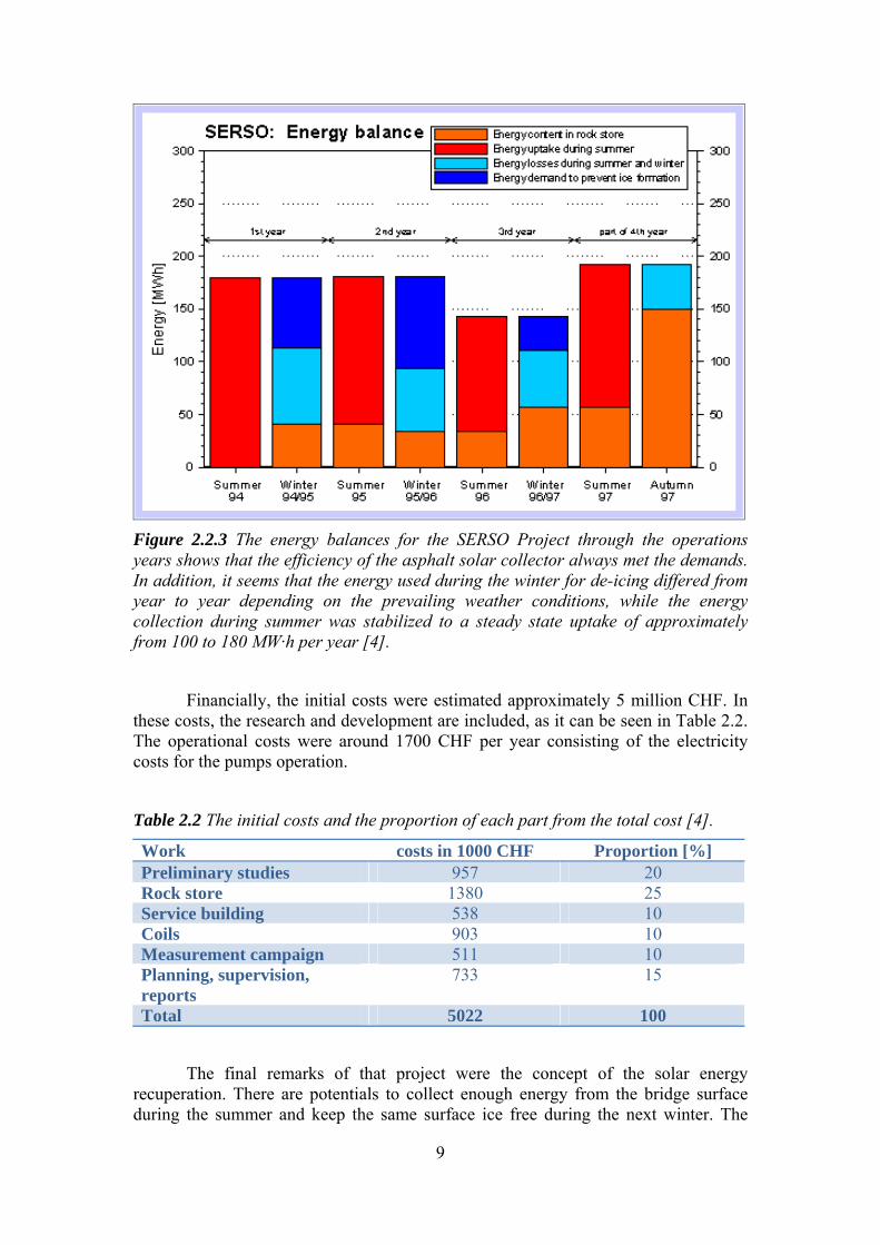
The most important result was found to be that the energy produced by the road was steady, with some variations, through the operation years and more than the energy used for the stabilization of the road temperature, as it can be seen in Figure 2.2.2. That means that the system was not only achieved its initial goal but also revealed it can be economically profitable for energy savings.

9

Figure 2.2.3 The energy balances for the SERSO Project through the operations years shows that the efficiency of the asphalt solar collector always met the demands. In addition, it seems that the energy used during the winter for de-icing differed from year to year depending on the prevailing weather conditions, while the energy collection during summer was stabilized to a steady state uptake of approximately from 100 to 180 MW·h per year [4].

Financially, the initial costs were estimated approximately 5 million CHF. In these costs, the research and development are included, as it can be seen in Table 2.2. The operational costs were around 1700 CHF per year consisting of the electricity costs for the pumps operation.

Table 2.2 The initial costs and the proportion of each part from the total cost [4].

Work costs in 1000 CHF Proportion [%] Preliminary studies 957 20 Rock store 1380 25 Service building 538 10 Coils 903 10 Measurement campaign 511 10 Planning, supervision, reports

733 15

Total 5022 100

The final remarks of that project were the concept of the solar energy recuperation. There are potentials to collect enough energy from the bridge surface during the summer and keep the same surface ice free during the next winter. The

10

SERSO project is an example of an effective energy recycling process of the solar energy that could be in any case radiated back to the atmosphere. The seasonal heat store and reuse can find more applications than keeping a surface ice free like for example in airports, sport stadiums, parking lots and ramps. This project has resulted in the research for the application of similar systems in the Airport of Vienna, a part of the highway in Berne, Switzerland and Geo VerSi for road safety in Germany.

2.3 TRL Report In the TRL report the use of inter-seasonal heat transfer systems was tested

with the incorporation of solar energy collectors in the asphalt roads and the corresponding insulated ground stores. Two solar heat collectors were constructed and two insulated heat stores with similar dimensions. One of the stores was installed under the street and the other besides it so as to simulate the scenario of retrofitting, as it can be seen in the scheme in Figure 2.3.1. The recovered heat from the asphalt road surface was evaluated in two ways, firstly for the maintenance of the road itself during the winter time and secondary for the heating of a nearby building. The cooling of the building was also investigated during the summer time with the removal of the excess heat.

Figure 2.3.1 Scheme showing the layout of the TRL trial [5].

The design, construction, operation and performance of the test methods for the heat recovery are included and explained thoroughly. The performance of the system was examined over a two years period with the intention for viewing the full seasonal assessments of the heat recovery from the road surface, the storage and its reuse for keeping snow and ice free the road surface during the winter. The time schedule and the purposes for each time period that has been followed can be seen in Figure 5.3.2.

11

Figure 2.3.2 The experimental schedule from September 2005 for two year period of operation [5].

The heat flow that was collected by each solar asphalt collector was determined by the volumetric flow rate of the pump and the fluid temperatures in the pipes flow. The temperature difference between the inlet and outlet temperature was used to calculate the heat recovered with the use of the following formula:

Where Q is the flow rate of the pump, c is the specific heat capacity, V the

volumetric flow rate and ΔT the temperature difference between the inlet and outlet temperatures. The specific heat capacity is depending on the temperature and the pressure of the fluid but in that case was assumed to be constant with a value of 4.046 J/gm/oC for a water and glycol mix. So in that case the formula was transformed into the following:

The heat transferred to the ground store was also measured in the same way.

In ideal conditions the heat collected from the asphalt collector would be equal to the heat stored although this is not the case in reality since losses occur during the operation and circulation of the fluid through the piping and pumping system.

The simulation of the energy collection from the road and/or the cooling of the building during the summer time and the heating injection during the winter, once for the road maintenance and once for building heating have been done with the use of computational protocols that were set. The measured temperatures and irradiation were measured every day by the weather station, that has been installed, and the variations can be seen in Table 2.3.1.

12

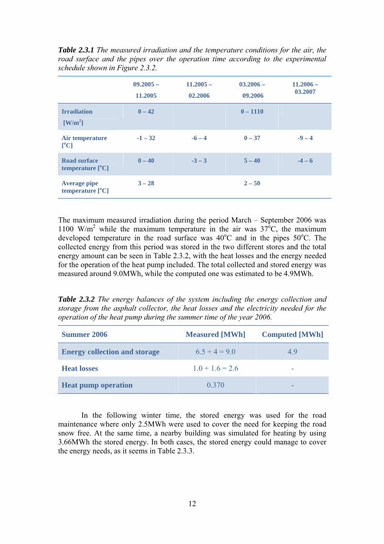
Table 2.3.1 The measured irradiation and the temperature conditions for the air, the road surface and the pipes over the operation time according to the experimental schedule shown in Figure 2.3.2.

09.2005 –

11.2005

11.2005 –

02.2006

03.2006 –

09.2006

11.2006 – 03.2007

Irradiation

[W/m2]

0 – 42 0 – 1110

Air temperature [oC]

-1 – 32 -6 – 4 0 – 37 -9 – 4

Road surface temperature [oC]

0 – 40 -3 – 3 5 – 40 -4 – 6

Average pipe temperature [oC]

3 – 28 2 – 50

The maximum measured irradiation during the period March – September 2006 was 1100 W/m2 while the maximum temperature in the air was 37oC, the maximum developed temperature in the road surface was 40oC and in the pipes 50oC. The collected energy from this period was stored in the two different stores and the total energy amount can be seen in Table 2.3.2, with the heat losses and the energy needed for the operation of the heat pump included. The total collected and stored energy was measured around 9.0MWh, while the computed one was estimated to be 4.9MWh.

Table 2.3.2 The energy balances of the system including the energy collection and storage from the asphalt collector, the heat losses and the electricity needed for the operation of the heat pump during the summer time of the year 2006.

Summer 2006 Measured [MWh] Computed [MWh]

Energy collection and storage 6.5 + 4 = 9.0 4.9

Heat losses 1.0 + 1.6 = 2.6 -

Heat pump operation 0.370 -

In the following winter time, the stored energy was used for the road maintenance where only 2.5MWh were used to cover the need for keeping the road snow free. At the same time, a nearby building was simulated for heating by using 3.66MWh the stored energy. In both cases, the stored energy could manage to cover the energy needs, as it seems in Table 2.3.3.

13

Table 2.3.3 The energy balances of the system during the winter time of the years 2006 to 2007 for the reuse of the stored energy that was collected during the summer. The stored energy was reused either for covering the needs of road maintenance or the heating demands of a nearby building.

Winter 2006 – 2007 Reused energy [MWh] Information

Road maintenance reused energy

2.5 Out of the 6.5MWh from store 1

Building heating reused energy

3.66 Heat pump COP = 2

The cost analysis of the installations and the heat recovery of the stored energy were also included and compared to the conventional techniques of salting the road surface for the winter maintenance. As a final conclusion it was stated that the interseasonal heat transfer system is successfully recovering the solar heat from the asphalt surface in the summer to store in insulated ground heat stores for reusing. The carbon footprint of such renewable energy technology is less than the vehicle operated salt spreading systems and traditionally powered building and cooling systems. As a recommendation, the encouragement of further research in the specific system was mentioned to be the only solution since the natural resources seem to be depleted as the time passes.

2.4 Worcester Polytechnic Institute Research The main interest of the research team in the WPI was the reduction of the urban heat island effect that usually happens in the center of the cities during the warmer periods of the year, which is responsible for the surroundings temperature increase and the cooling energy demands of the buildings and the emissions increase. The heat island effect reduction concept has been approached with the removal of the heat energy from the asphalt pavements through harvesting. That could be succeeded with a fluid’s flow through a piping system through high conductive layers which will absorb the heat and remove it from the pavements. A series of experiments in the laboratory and simulations has been done to examine the different influencing parameters so as to achieve the most optimum result.

Firstly, a small scale experiment was conducted in the laboratory for the optimization and control of the spacing and the configuration of the pipes. Following, there was a large scale experiment that has been conducted with outdoor conditions and also a simulation to compare the results. A slab was prepared with copper pipes installed and was placed outdoors, where the weather conditions such as the wind speed of 1.05 m/s and the solar radiation of 255 to 800 W/m2 were measured. The temperatures in the asphalt were measured in different locations on the surface of the asphalt and in inner layers versus time. These parameters and their effects are shown in Table 2.4.

14

Table 2.4 Parameters examined in a small case experiment for the direct heat reduction of the asphalt surface.

Parameter Effect

Pipe spacing The closer the spacing, the better the reduction of temperature. See Figure 2.4.1.

Pipe configuration The more closely pipes are used, the more the reduction in the surface temperature surface will be. That was proved with the comparison of serpentine versus straight pipes.

Thermal conductivity of the pavement

The thermal conductivity of the aggregates influences the thermal conductivity of the asphalt mix and so on the temperature increase in the outlet flow of the pipes. The quartzite was found to be more favorable to the limestone in the asphalt mix. See Figure 2.4.2.

Piping material The copper pipes have been compared to plastic pipes to result in the conclusion that some plastic pipes are more efficient in the heat extraction than the copper ones. The plastic pipes are considerably cheaper than the copper ones and that makes them even more attractive. See Figure 2.4.3.

Figure 2.4.1 Effect of pipe spacing on the reduction of temperature in the surface of the asphalt pavement [6].

15

Figure 2.4.2 Comparison of the aggregate types and the difference in the inlet and outlet water from the asphalt collector sample [6].

Figure 2.4.3 Comparison of the piping material types and the difference in the inlet and outlet water from the asphalt solar collector sample [6].

The efficiency of the systems was defined as the extracted heat flow of a pipe to the initial solar irradiation to the system according to the following formula:

Where M is the mass flow rate of the water in kg/s, C is the specific heat capacity of the water in J/Kg·K, Tout is the temperature of the outgoing water in oC, Tin is the temperature of the incoming water in oC, G is the solar irradiation in W/m2 and A is the area of heat conduction in m2; i.e. π x pipe diameter x pipe length.

In addition, the economical analysis has been managed in accordance with the American prices. The main conclusions made can be rounded in the following ones.

16

1. There is feasibility of removing heat energy from the pavements according to the experimental and simulation results, which can be used for the reduction of the heat island effect.

2. The reduction in the pavement’s temperature is dependent on the location and spacing of the pipes.

3. The reduction of the pavement’s temperature increases the life time of the pavement.

4. The use of high conductive layers can be used to reduce the number of pipes.

2.5 Road Energy Systems In order to investigate the opportunity to collect solar energy from the asphalt

temperatures, a number of Dutch companies found the Road Energy Systems in 1997. The system works during the summer to collect the energy from the pavements through cold water that is pumped up from an underground aquifer to the asphalt collector. The warmed water is transferred then through a heat exchanger to another underground store. The purpose it to cool down the pavements during the summer for reducing the rutting and to heat them during the winter for snow free conditions. If a building is introduced to that system then the cooling and heating demands can be covered in the same way they are done for the asphalt surface, as it seems in Figure 2.5.1.

Figure 2.5.1 Application of the asphalt solar collector by the Road Energy Systems [7].

The methodology has been developed after testing that was carried out in Hoorn, the Netherlands between 1998 and 2001. Temperature measurements at about 150 locations of different operating systems were collected and used to a computational tool (RES-design) so as to examine the optimization of the system’s performance and form a typology of the alternative designs. In the following Figures 2.5.2 to 2.5.3 the different parameters that the system depends on are shown and

17

indicate the range of the potential energy output that can be managed with the use of different design.

Figure 2.5.2 Typical example of input and output temperatures [7].

Figure 2.5.3 Example of average output temperature curve for Dutch climatic conditions [7].

18

Figure 2.5.4 Example of annual energy output curve for Dutch climate conditions [7].

The aspects of the road construction in the development phase has examined and considered the traffic load, the surfacing layers and the durability under the mechanical loadings. It has been suggested that the construction of an asphalt solar collector should be probable done in a short time period so as to be able to apply it in existing pavements that are in use. The system that has been finally the optimum one to use after different studies is shown in Figure 2.5.5.

Figure 2.5.5 Overview of the developed asphalt solar collector system [7].

19

Figure 2.5.6 Stress concentration in the asphalt mix [7].

From the engineering point of view, the mechanical load has been considered for the stresses concentration around the pipes and the possibility of damaging them. The advantage of increased temperature when the pipes are placed close to the surface can be subsided by the risk of life time decrease. The placement of the piping system on depth and the developed principal stresses in the asphalt near the pipes are shown in Figure 2.5.6. This problem has been solved with the use of relatively soft asphaltic mix and use of interlocking grid that give the asphalt higher resistance against the crack growth. In that case the pipe can be still kept close to the surface excluding the risk of cracks and apply the possibility of an easier future removal of the piping system.

The Road Energy Systems has found application to several projects in the Netherlands, and also abroad and the experience that has been gathered through the practice has given standardization to the dimensions of a system. For example, an office building with a space of 10000m2 requires an asphalt collector of 4000 m2, energy storage with a pumping capacity of 110m3/h and a heat pump capacity of 340kW. Such a system can produce 55% less CO2 than a conventional gas heated and air conditioned office building and use 55% less fossil fuels for heating and cooling.

20

2.6 Studies comparison Each one of the above projects has been studied in accordance with the climate data of the area located to, where the variation of the solar irradiation, the air temperature and the wind load were different. The thermal energy store systems they used for interseasonal storage were different types of ground source heat pumps. The reuse of the collected and stored energy was different for each case and had an annual energy output that was an energy demand for each case as it can be seen in Table 2.6.

Table 2.6 Concentrating table of the different asphalt solar collector projects and their main characteristics.

SERSO TRL WPI Road Energy

Location Switzerland

England West USA The Netherlands

Seasonal thermal energy storage

Vertical Ground source

heat pump

Thermal insulated

underground tank

None Groundwater heat pump (Aquifer)

Annual energy output from the solar asphalt collector [kWh/m2]

77 – 138.5

60

167

18.5

21

3 SOLAR ENERGY AND TEMPERATURE

3.1 Solar energy potentials The heat requirements of the Fågelsten residential area have to be met by the new system. A typical solution in Swedish urban areas is to connect the buildings to an existing district heating system, often based on biomass and/or waste heat. Others alternatives are e.g. local heating plants based on biomass boilers or ground source

heat pumps. Solar energy is one possibility to design a heating system. However, the usual problem with this energy is its availability compared to the general heat demand time. The heating needs are high in winter and the irradiation from the sun is higher in the summer. That is the reason why a seasonal storage system is needed. Moreover, the intermittency of solar system between days and nights make them less convenient at the end. The typical solar energy distribution on the surface of the Earth and the losses to the atmosphere can be seen in Figure 3.1.

Figure 3.1 The solar energy distribution in the Earth [8].

22

3.2 Solar irradiation The radiation from the Sun reaching the Earth generates heat on the ground.

The solar irradiation depends on the latitude and the angle of incidence. From a meteorological perspective, the irradiation variations in Europe are shown in the Figure 3.2.1 for horizontal surfaces and as it seems the central and northern Europe is being exposed to an irradiation between 2000 and 3000 Wh/m2 per year according to the measurements of the Joint Research Center.

Figure 3.2.1 The average annual solar irradiation variations in Europe for horizontal surfaces [9]. From an energy perspective, in the south Sweden, the maximum global solar irradiation that can be translated into a term of potential energy use is about 1100 kWh/m² and year, while it usually ranges from 1000 to 1500 kWh/m² per year. In the asphalt collector case for the residential area in Fågelsten, the angle of incidence does not matter, since it is a horizontal surface. For Säve, Göteborg the NASA gives an annual average irradiance value of 126.3 W/m² while the average monthly variations can be seen in Figure 3.2.2 for both solar radiation and irradiation.

23

Figure 3.2.2 The average monthly solar irradiation and radiation for horizontal surfaces in the Earth measured by NASA [10].

24

3.3 Temperature profiles The solar irradiation and the way it affects the ambience is influenced by several parameters such as the prevailing winds, the humidity and the precipitation, the consequently wet days, the days with frost, the hours of sunny days and clear sky. All the above parameters are variables on which the air temperature depends and varies from minimum to maximum temperatures and can be approached with an average value, as it can be seen in Figure 3.3.1 for the city of Göteborg. In Table 3.3.1 the variations of the air temperature can be found to be from -0.3 to 16.6oC.

Figure 3.3.1 The complete graph of climate information for Göteborg [11]. The average Earth temperature at the surface is slightly above the average air temperature due to the absorption of solar heat the underground heat from the inner Earth. In fact, the upper soil cover of the Earth is acting as insulation minimizing the temperature fluctuations and showing a constant temperature profile after approximately 10 meters of depth, as it can be seen in Figure 3.3.2. In the same figure the temperatures in 100 meters depth in Sweden shows that Göteborg’s underground temperature is estimated to be constant around 8oC while the surface’s temperature varies from 2 to 17.5oC, as Table 3.3.1 shows. The earth is warmer than the air during the winter and colder than the air during the summer leading to the concept of using the Earth as a heating and cooling system for buildings.

25

Figure 3.3.2 Typical soil temperature variation and the bedrock temperature profile of Sweden in 100 meters depth. Göteborg is located on the line that indicates a temperature of 8oC at this depth [8], [12].

The asphalt can be compared to a black body, whose absorptivity is very close

to one, the temperature could be even higher. That is the reason why the asphalt, a black surface, is convenient to absorb solar heat and that explains a higher surface temperature for asphalt area. The asphalt temperature variations are being measured by the Trafikverket, which is the traffic agency of Sweden. For the Fågelsten case the asphalt temperature measurements have been taken from Fiskebäck’s VViS station, which is located in west of Frölunda, for the year 2009 are the shown in the table 3.4.1. Unfortunately, there were no data measured for the month December due to malfunction of the local weather station.

The average monthly air, earth and asphalt temperatures are shown in Table 3.3 and Figure 3.3.3. This graph shows that whereas the air mean temperature is between 14 and 17oC during the summer, the asphalt pavement temperature reaches 25oC in average according to the Trafikverket data.

26

Table 3.3 The average monthly variations for the air and the earth temperature and the differences between their measured values by NASA and Trafikverket [10], [13]. Month Air temperature

[°C] Earth temperature

[°C] Asphalt temperature

[°C]

January -0.3 2.0 0.7

February -0.7 1.2 1.8

March 1.9 2.4 4.6

April 5.9 5.7 14.4

May 11.0 10.6 22.1

June 14.2 14.8 25.2

July 16.6 17.2 24.8

August 16.1 17.5 25.0

September 12.1 14.4 15.3

October 8.6 10.7 7.5

November 3.8 6.9 5.1

December 1.1 3.6 -

Figure 3.3.3 The average air, ground and asphalt temperature variations.

27

4 SYSTEMS AND COMPONENTS

4.1 Solar collectors These systems use collectors to capture the heat from the solar radiation. That

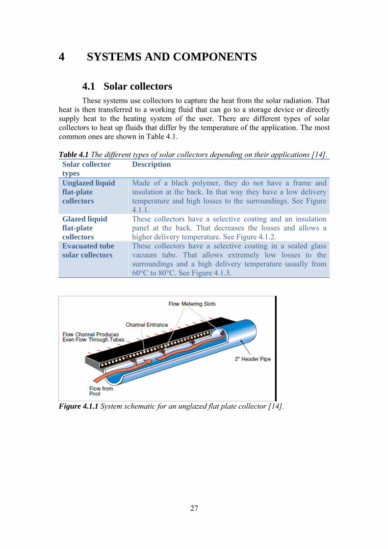
heat is then transferred to a working fluid that can go to a storage device or directly supply heat to the heating system of the user. There are different types of solar collectors to heat up fluids that differ by the temperature of the application. The most common ones are shown in Table 4.1. Table 4.1 The different types of solar collectors depending on their applications [14]. Solar collector types

Description

Unglazed liquid flat-plate collectors

Made of a black polymer, they do not have a frame and insulation at the back. In that way they have a low delivery temperature and high losses to the surroundings. See Figure 4.1.1.

Glazed liquid flat-plate collectors

These collectors have a selective coating and an insulation panel at the back. That decreases the losses and allows a higher delivery temperature. See Figure 4.1.2.

Evacuated tube solar collectors

These collectors have a selective coating in a sealed glass vacuum tube. That allows extremely low losses to the surroundings and a high delivery temperature usually from 60°C to 80°C. See Figure 4.1.3.

Figure 4.1.1 System schematic for an unglazed flat plate collector [14].

28

Figure 4.1.2 System schematic for a glazed flat plate collector [14].

Figure 4.1.3 System schematic for an evacuated tube solar collector [14].

4.2 Ground source heat pumps The ground source heat pumps are one of the fastest spreading sustainable

energy systems worldwide. The main principle is to take the free heat, coming from the sun and absorbed in the ground, concentrate and upgrade this heat thanks to a heat pump. The facts that the ground conductivity is relatively low and the heat storage capacity is rather high imply that the ground temperature is changing slowly. That is the reason why the transfer of heat over different seasons, winter and summer mainly, is possible. In addition, in a few meters depth the ground is considered to be insulated

29

and the temperature almost constant with a low amplitude of variation over a year. That makes the possibility of seasonal storage system feasible.

The ground source heat pumps use the free heat from the ground to supply heating and cooling to the buildings. A ground source heat pump can enhance the heating with a coefficient of performance, which compare the heat movement to the useful work input. That is why the average COP can vary from 2.4 to 5 depending on the type of ground source heat pump.

A heat pumps work by following a compression cycle composed of four main components which are: a compressor, an expansion valve and two heat exchangers; the evaporator and the condenser. A working fluid circulates in that closed circuit that can be seen in Figure 4.2.1. Starting in the evaporator, the fluid absorbs heat by being evaporated. Then the vapour is compressed in order to increase both temperature and pressure. The vapour arrives in the condenser where it comes back to liquid state by releasing heat to the building. The liquid is expanded by the expansion valve to reduce both temperature and pressure.

Figure 4.2.1 Refrigeration cycle in heating mode of a typical heat pump [15].

A ground source heat pump differs from a refrigerator by being able to run in both directions: heating and cooling mode. This can be done thanks to a reversing valve. The heat pump needs a sufficient temperature difference between the heat pump and the earth connection. Otherwise, the heat could flow in the wrong direction

The COP (Coefficient of Performance) of a heat pump using Carnot cycle is:

30

The real COP is usually 50-60% of the Carnot COP, which is called in our case, the refrigeration cycle is used for a ground source heat pump only for heating purpose. Knowing that, the evaporator takes the heat from the solar collector and the condenser releases the heat to the building. For a giving supply temperature, the COP can be improved by decreasing the temperature lift. It can be done by increasing the evaporator temperature.

There are different types of ground source heat pumps according to the connection is used. A ground source heat pump extracts heat from the Earth in general, and it is called the “earth connection”. That connection can be the ground, the ground water or the surface water. The most used type of earth connection is the one using vertical boreholes in the ground. But horizontal systems are also used. “Open loop” and “closed loop” system can also be distinguished by the fact that the system always use the same fluid for each cycle or use a natural well to take the heat and a natural sink to return it. The ground source heat pumps are presented and described in Table 4.2, while in Figures 4.2.2, 4.2.3 and 4.2.4 schemes of these types are shown.

Table 4.2 The different types of ground source heat pumps and the description of their main characteristics [8]. GSHP types Description Ground-Coupled Heat Pumps (GCHPs)

This type uses the ground as a heat source or sink. It can be vertical or horizontal ground heat exchangers. See Figures 4.2.2 and 4.2.3.

Groundwater Heat Pumps (GWHPs)

This type uses underground water called aquifer as a heat source or sink. See Figure 4.2.4.

Surface Water Heat Pumps (SWHPs)

This type uses surface water bodies such as lakes, ponds etc.

Ground Frost Heat Pumps (GFHPs)

This type uses the ground around foundation in areas with permafrost for cooling purposes.

31

Figure 4.2.2 Vertical heat exchanger of Ground Couple Heat Pump System [8].

Figure 4.2.3 Horizontal heat exchanger of Ground Couple Heat Pump System [8].

Figure 4.2.4 Ground Water Heat Pump System [8].

32

4.3 Thermal storage systems The storage or thermal energy makes energy systems more effective by extracting

and storing heat when it is the most efficient and then re-use the heat by taking back the heat from the storage device. In that way the use of renewable can be made in a more efficient manner. The thermal storage systems are presented and described in Table 4.3, while in Figure 4.3.1 schemes of these types are shown.

Table 4.3 The different types of thermal storage systems and the description of their main characteristics [8]. TES types Description Underground Thermal Energy Storage (UTES) Closed systems They use the same fluid for each cycle. The

common system is called BTES (Borehole Thermal Energy Storage). See Figure 4.3.2.

Open systems They use natural heat well and sink. ATES (Aquifer) and CTES (Cavern). Their main advantage is a higher heat transfer capacity. See Figure 4.3.1.

Water tanks This is the best known energy storage system and mostly used with solar collectors.

Phase Change Materials (PCMs)

This system uses the change of phase of a material, such as freezing, melting or vaporization in order to store energy. Then temperatures and pressures for the charge and discharge phases have to be well chosen.

Figure 4.3.1 Open Loop system connected to an aquifer [16]. Figure 4.3.2 Closed Loop system. The closed loop systems can be vertical, horizontal or connected to a pond or a lake [16].

33

4.4 Combination of ground source heat pumps and solar collectors

The main principle is to combine the advantages of both systems in order to create new operational conditions for both systems. The solar collectors can produce energy and then store it in the boreholes; the system then is usually called geosolar or combisystem, as it show in Figure 4.4. Even at a low temperature compared to conventional solar collector acting alone, it will be able to recharge the boreholes in a more efficient way. As a matter of fact, the efficiency will be better due to a lower temperature. While it recharges the boreholes, it will increase the fluid temperature, and thus bring the possibility to use shorter boreholes and extract more heat from the boreholes. Another advantage is the decrease of the interaction between adjacent boreholes, which will result in lower losses in the ground and better system efficiency.

Figure 4.4 Geosolar system from Karlsruhe, Germany, with flat plate solar collectors for domestic hot water DHW and unglazed solar collectors connected to the ground heat exchanger pump [12].

The combination between the two systems can be done differently depending on the type of regulation system, as it seems in Table 4.4. As a matter of fact the control strategy can be rather different, and thus resulting in quite different heat distribution and operational conditions for the heat storage, the hot water supply and the heat pump. During the year of 2001, half of the domestic solar collectors that were installed in Austria, Denmark, Norway, and Switzerland were for combisystems, while in Sweden it was more. Combisystems started being used in Canada since the

34

mid 1980s. Some of these systems can incorporate solar thermal cooling during the summer time in addition.

Table 4.4 Different possible ways to use a solar energy with ground source heat pumps [12]. Operation mode Solar collector Heat pump Borehole system The solar collector is being used directly to supply DHW and heating to the building.

Heat production at high temperatures is required to supply the DHW and the heating to the building.

The heat pump is not in operation most of the time. It is used when the solar collector is not enough.

Reduced heat extraction, since the heat pump is only used during peak loads.

The solar collector is being used to produce heat for recharging the borehole.

Heat production at lower temperatures, gives increased efficiency and longer operation time.

The heat pump is in operation, with an increased COP because of the high temperature to the evaporator, and can decreases the operation time.

The heat injection to the borehole gives increased temperatures, especially for the evaporator part of the heat pump.

Concerning the second operation mode, it can be divided into two sub modes, which are a continuous flow through the solar collector, the boreholes and the heat pump or a by-pass of the heat pump, which consists in a closed loop between the solar collector and the boreholes.

The case of the asphalt solar collector is a new sort of system that appears to be interesting compared to the solar water heating systems described above for energy, economical and environmental reasons. In the next chapter, a review of a several existing systems is following in order to give a global overview of this system and its main characteristics such us the energy collection, the costs involved and the possible construction processes.

35

5 BUILDING ENERGY DEMANDS

5.1 Domestic energy consumption principles The energy demands for a building can be specified in the energy consumed

during the construction and the energy consumed during the life time of the building. The latest can be named domestic energy consumption and is dependent on the construction method and the climate of the location. That means that the insulation and the air-tightness will manage to maintain a stable indoor climate independent of the temperate outdoor climate of Sweden and consequently the domestic energy consumption. This principle applies in the idea of the passive house design and the effort for green and sustainable buildings.

The domestic energy consumption is defined as the amount of energy used for the different appliances in a household. The average energy used within a typical house in a typical temperate climate is approximately 20 MWh per year. This amount is dependent on the location, the weather and the size of the housing electricity and the tenants use. The yearly use of the domestic energy consumption for different uses in temperate climates is shown in Table 5.1 and the comparison between them in Figure 5.1.

Table 5.1 Average domestic energy consumption per household in temperate climates [17].

Domestic energy use Average consumption [MWh/yr]

Heating 12

Hot water 3

Cooling refrigeration 1.2

Lighting 1.2

Washing and drying 1

Cooking 1

Miscellaneous electric load 0.6

Total 20

36

Figure 5.1 Comparison between the household energy consumption uses, which shows that the heating of a household demands even more than half of the total energy consumption.

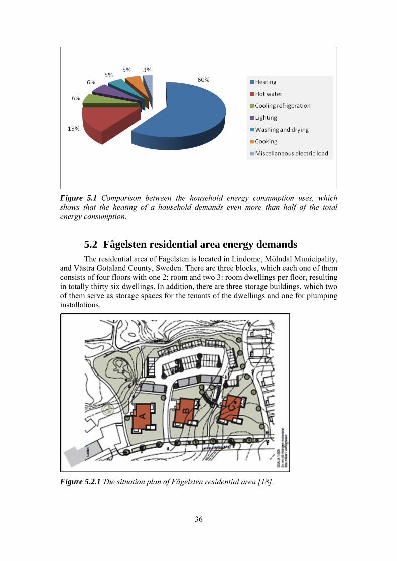
5.2 Fågelsten residential area energy demands The residential area of Fågelsten is located in Lindome, Mölndal Municipality,

and Västra Gotaland County, Sweden. There are three blocks, which each one of them consists of four floors with one 2: room and two 3: room dwellings per floor, resulting in totally thirty six dwellings. In addition, there are three storage buildings, which two of them serve as storage spaces for the tenants of the dwellings and one for plumping installations.

Figure 5.2.1 The situation plan of Fågelsten residential area [18].

37

The energy demands have been calculated by NCC with the use of the “Enorm 2004” software. The area of the buildings has been divided into two zones because of the different indoor climate demands; these are the flats and the storage buildings. The indoor climate has been designed with regards to the Building Administration and NCC’s standards. In that case the specific energy demands for a building is the maximum 90 kWh per m2 of heated area and year for NCC and 110 kWh per m2 of heated area and year for the Building Administration, while the average building’s envelope U-value is the least 0.5. Furthermore, there were set standards for the temperatures, the ventilation, the hot water demands, the leakages etc. where they can be found in request at NCC, whereas a general summary is provided at Annex I.

The results from the “Enorm 2004” software show the consumption for each zone for the heating, hot water, miscellaneous electrical load and other demands. The energy consumption of the whole residential area is estimated to be approximately 120 MWh/year. It has to be noted that it is not easy to estimate the energy consumption per household since the size of the dwellings differs from one another so in that case it was preferred to use the total energy consumption of the whole residential area. In Table 5.2 the energy consumption of each domestic use can be seen.

Table 5.2 Average domestic energy consumption in Fågelsten.

Domestic energy use Average consumption [MWh/yr]

Heating & domestic hot water 69.8

Others (FTX and pump electricity) 11.4

Household electricity 37.7

Total 118.9

In Figure 5.2.1 the comparison between the uses shows that the heating demands are the prevailing ones in the total domestic energy consumption at 55%, which is relevant close to the percentage as it has been shown in Figure 5.1.

38

Figure 5.2.2 Comparison between the household energy consumption uses for Fågelsten residential area, which shows that the heating demands approximately the half of the total energy consumption.

The district heating is the common way for heating the buildings in Sweden and the usual choice of NCC. In the following Figure 5.2.3, there is the energy consumption for the heating by the district heating in comparison to the electricity demands for the FTX ventilation system, the pump and the household. The heating is covering most of the total energy consumption, except for the summer months that the use is decreased only for the hot water needs. It is obvious though that the total energy use for the heating is the most important one and consequently dependent to the district heating. That means if the district heating increases the cost then the energy expenses of a household in total will be also increased.

Figure 5.2.3 The domestic energy consumption in total and separately for Fågelsten residential zone through the year.

39

6 ASPHALT SOLAR COLLECTOR

6.1 Theory 6.1.1 Analytical approach

The differential form of Fourier’s Law of thermal conduction shows that the local heat flux, , is equal to the product of thermal conductivity, k, and the negative local temperature gradient, . The heat flux is the amount of energy that flows through a particular surface per unit area per unit time according to the following formula:

Where

• is the local heat flux in W/m2,

• k is the material’s conductivity in W/m K, and

• is the temperature gradient in K/m.

In the three dimensional coordinate system it is expresses to each direction as the following formulas:

Though in many simple applications, Fourier’s law is used in its one dimensional form in the x-direction.

The thermal conductivity, k, is a thermophysical property of the substance through which the heat flows and is usually expressed in W/m·K. It is directly related to the microscopic mechanism in the transfer of heat within the matter. In isotropic materials it is considered as a constant while in anisotropic materials it varies with orientation and in nonuniform materials it varies with spatial location.

Conduction – The heat transfer by conduction is the energy transfer through asubstance, a solid or a  fluid as result of the presence of a temperature gradientwithin the substance. This process is also referred to as the diffusion of energy orheat  [19]. The  law of Heat Conduction, also known as Fourier’s  law, states  thatthe time rate of heat transfer through a material  is proportional to the negativegradient  in  the  temperature  and  to  the  area  at  right  angles,  to  that  gradient,through which the heat is following [20]. 

40

The convection heat transfer can be expressed by Newton’s law of cooling as the heat flow, Q, with the following formula [19]:

It can also be expressed as the heat flux, q, with the following formula:

Where

• A is the surface area of the body which is in contact with the fluid in m2,

• ΔT is the appropriate temperature difference,

• q is the heat flux, and

• h is the convection heat transfer coefficient in W/m2K.

The heat transfer convection cooling can be divided into four main categories depending on the conditions under it happens, so it can be natural or forced, and on the type of geometry, so it can be internal or external convection flow. In addition to the above categories, the laminar or turbulent flow conditions can be taken into consideration resulting in a total of eight convection types, as it is shown in Figure 6.1.2.

The natural from the forced convection differs in the fact that the later one a flow is being created by an external force. In the natural convection, buoyancy forces created by temperature gradients and the consequent thermal expansion of the fluid lead the flow’s movement.

The heat transfer coefficient, h, is given by various relationships depending on the convection type it expresses. The heat transfer coefficient is not constant and varies with the geometrical shape, the ambient temperature and the wind conditions. Many heat transfer handbooks uses though the dimensionless numbers for the approach of the heat transfer coefficient as they are shown in Table 6.1.2.

Convection – The heat transfer by convection is the energy transfer between afluid and a solid surface. Heat transfer by convection  is more difficult to analyzethan the heat transfer by conduction because it varies from situation to situationupon  the  fluid  flow  conditions.  In  practice,  the  heat  transfer  by  convection  istreated empirically [21]. 

41

Figure 6.1.2 The eight possible convection types [20].

Table 6.1.2 Empirical and theoretical expressions for the h coefficient [20].

Expression Empirical/theoretical expressions

(1) Nusselt number

(2) Reynolds number

(3) Grashof number

(4) Prandtl number

(5) Rayleigh number

Where

• h is the heat transfer coefficient in W/m2·K,

• L is the characteristic length,

• ΔT is the temperature difference between surface and cooling fluid bulk in K,

• g is the gravitational constant in m/s2,

• k is the thermal conductivity of the fluid in W/m·K,

• ρ is the fluid density in kg/m3,

• U is the bulk velocity in m/s,

42

• η is the viscosity in Pa·s,

• g is gravitational acceleration in m/s2,

• denotes the temperature of the hot surface in K,

• equals the temperature of the surrounding air in K,

• Cp equals the heat capacity of the fluid in J/kg·K, and

• β is the thermal expansivity in 1/K.

In the case of forced convection, where the flow is driven externally, the nature of the flow is characterized by the Reynolds number, Re, which describes the ratio of the inertial forces to the viscous ones. According to the expression (2) in Table 6.1.2, the Reynolds number depends on the velocity, the viscosity, the density and the length scale.

However, in the case of natural convection, where the flow is driven internally, the nature of the flow is characterized by the Grashof number, Gr, which describes the ration of the internal driving or buoyancy force to a viscous force acting on the fluid. According to the expression (3) in Table 6.1.2, the Grashof number depends like the Reynolds number on the length scale, the fluid’s physical properties and the temperature scale. For ideal gases, the expansion coefficient is given by .

The transition from a laminar to a turbulent occurs at a Gr value of 109, whereas the flow is considered to be turbulent for greater values.

The h coefficient is based on the Nusselt number correlations from handbooks and is expressed as a function of the material properties, the flow rate and the geometry. According to the expression (1) in Table 6.1.2 it seems that h is rather complicated and it depends on the Reynolds, Prandtl and Rayleigh numbers and expression (1) can be the approach as an average solution for the h coefficient. A more general correlation [22] for the natural convection case that applies for a variety of geometries is:

The value of f4(Pr) is calculated with the use of the following formula:

Where Nu0 values vary from 0.54 to 0.68 depending on the geometry of the surface.

43

The rate of energy emitted by an ideal surface, black body, with emissivity equals to 1 is given by Stefan-Boltzmann’s law:

Where Eb is the rater of black body radiation energy, ε is the emissivity of the material and σ is the Stefan-Boltzmann’s constant equal to 5.68x10-8W/m2K4 and T is the temperature of the surface.

6.1.2 Energy balance of an asphalt pavement The heat energy transfer from the sun’s radiation to an asphalt pavement can be depicted by the energy balance theory, where all the different parameters and mechanisms of heat transfer take place and correlate to each other, as it can be seen in Figure 6.1.3; in Table 6.1.3 the description and the empirical expressions of each parameter are shown.

Figure 6.1.3 The energy balance on the surface of an asphalt pavement.

Radiation – The  transfer of energy by electromagnetic waves  through emptyspace  is  called  radiation  heat  transfer.  Energy  can  be  transferred  by  thermalradiation between a gas and solid surface or between two or more surfaces [19].All objects with a temperature greater than absolute zero will radiate energy at arate equal to their emissivity multiplied by the rate at which energy would radiatefrom them if they were a black body [23]. 

44

Table 6.1.3 The different parameters involved in the energy balance on an asphalt pavement, the empirical expressions and the descriptions [19].

Parameter Empirical expression

Description

(1) Irradiation

It is defined as the amount of radiation energy reaching a surface. The irradiation per unit area is defined as G in W/m2. λ denotes the monochromatic rate of radiant energy reaching the surface.

(2) Absorptivity

It is defined as the fraction of the total incident radiation that is absorbed by the surface. The absorptivity varies with the wavelength so the monochromatic absorptivity is denoted as αλ. The asphalt mixtures absorptivity α usually varies from 0.85 to 0.98.

(3) Reflectivity

It is defined as the fraction of total incident radiation that is reflected by the surface. The reflectivity is dependant of a wavelength function ρλ.

(4) Transmissivity

It is defined as the fraction of the total incident radiation that is transmitted through the body. It is dependant of a wavelength function τλ. For most of the solid surfaces the τ equals to zero since the bodies are usually opaque to the incident radiation.

(5) Emissivity

It is defined as the ration of energy radiated by the material to energy radiated by a black body at the same temperature. It expresses the ability of a material to absorb and radiate energy. A true black body’s ε equals to 1 while the rest less than 1. It depends on a wavelength function ελ, the temperature and the emission angle.

(6) Radiosity

It is defined as the amount of thermal radiation leaving a body. It is the sum of the incident radiation reflected and emitted away of a body in W/m2.

45

The total sum of the absorptivity, the reflectivity and the transmissivity is equal to one.

As it is stated in parameter (4) in Table 6.2.1, the transmissivity equal to zero for an opaque body.

So the initial sum becomes

Moreover, for a black body the absorptivity equals the emissivity. The emissivity, and hence the absorptivity, in the asphalt mixes varies from 0.85 to 0.95.

6.1.3 Finite elements analysis of the energy balance on the asphalt pavements

In a finite element analysis there should be two main things to be specified; the governing equation, which in that case is the heat equation, and the boundary conditions, which specify the heat transfer mechanisms. The general heat equation and the boundary conditions are expressed in the following paragraphs, according to the main theories described in [20].

The Heat Equation

The fundamental law finds that is being used and governing the heat transfer is the first law of thermodynamics, which is usually mentioned as the principle of energy conservation. The internal energy, U, though cannot be measured so it is hard to be included in the simulations. For this reason, the basic law is being transformed into an equation depending on the temperature, T, and for a fluid the heat equation is expressed as:

Where

• ρ is the density in kg/m3

• Cp is the specific heat capacity at constant pressure in J/kg·K

46

• T is the absolute temperature in K

• u is the velocity vector (m/s)

• q is the heat flux by conduction in W/m2

• p is the pressure in Pa

• τ is the viscous stress tensor in Pa

• S is the strain rate tensor in 1/s and expressed as:

• Q contains heat sources other than viscous heating in W/m3.

Inserting Fourier’s law in the heat equation, and ignoring the viscous heating and pressure work puts the heat equation on a more familiar form:

The above equation is being solved for the temperature, T. The convective heat transfer is left on the users choice to be activated or not, and when it is included then the velocity u can be entered as a mathematical expression of the independent variables or calculate it within COMSOL Multiphysics. If the velocity is set to zero, then the equation gets the pure conductive heat transfer in a solid:

The Boundary Conditions

The heat equation has two basic boundary condition types; specified temperature and specified heat flux. The last one is of Dirichlet type and prescribes the temperature at a boundary:

on

While the latter specifies the inward heat flux and taking into account the radiation

on

47

Where

• q is the total heat flux vector in W/m2:

• n is the normal vector of the boundary

• q0 is the inward heat flux in W/m2, normal to the boundary.

The above boundary condition can change forms in special cases. These are:

• for thermal insulation

• for convective flux, or the equivalent form of

• .

If the velocities are zero, thermal insulation and convective heat flux are equivalent conditions.

The inward heat flux q0 is normally a sum of contributions from different heat transfer processes. It is often convenient to split the heat flux boundary conditions as:

on

Where qr corresponds to the incoming radiation while the last term is the heat transfer between the surface temperature T and a reference temperature Tinf.

6.2 Modeling The finite element analysis has been conducted by the use of the COMSOL Multiphysics and especially with the General Heat Transfer application mode. The method that has been used follows the heat transfer theory and it is being further explained in the next paragraphs.

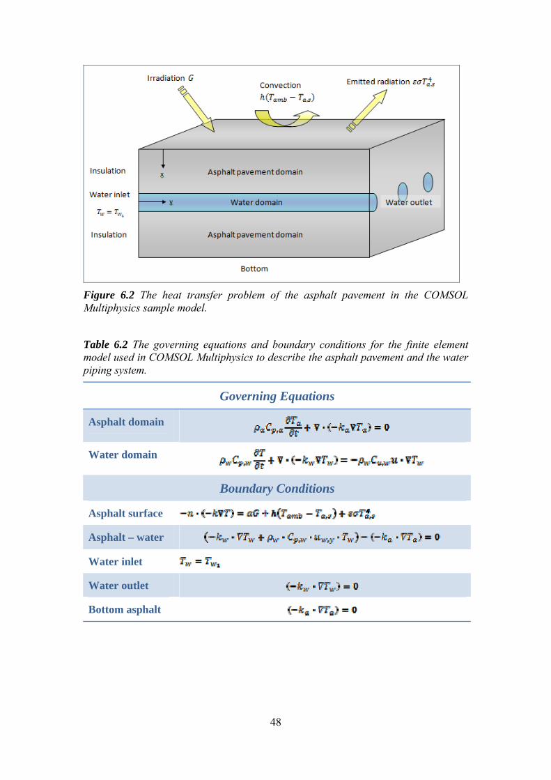
6.2.1 The asphalt pavement model The heat transfer problem is a combination of heat conduction, convection and radiation problem with boundary conditions at pavement – air and pavement – water interface, as is shown in Figure 6.2. The problem consists of two domains; the asphalt pavement domain where the heat transfer conduction is solved and the water domain where the convective terms are taken into account. The governing equations for the asphalt and water domain and moreover the boundary conditions in the interfaces and the external boundaries are given in the Table 6.2.

48

Figure 6.2 The heat transfer problem of the asphalt pavement in the COMSOL Multiphysics sample model.

Table 6.2 The governing equations and boundary conditions for the finite element model used in COMSOL Multiphysics to describe the asphalt pavement and the water piping system.

Governing Equations

Asphalt domain

Water domain

Boundary Conditions

Asphalt surface

Asphalt – water

Water inlet

Water outlet

Bottom asphalt

49

6.2.2 The geometry of the base case model Firstly, a basic case model was chosen so as it could be part of a more extended model but still able to depict the main function of the solar energy capture and transfer of that energy as heat through the piping system. The dimensions of the asphalt pavement were 20 meters for the length, which is the width of the parking lot area in Fågelsten, 1.5 meters for the width and 0.3 for the depth, as it is shown in Figure 6.2.2.

Three pipes were placed in the sample model so as to examine the intermediate one and the way the other two affect it. The pipes were placed initially 15mm below the asphalt surface, while the spacing between them was 200mm and the diameter of the pipes was 20mm. The rest of the properties are described in the following paragraphs. It has to be noted that the inlet temperature is not constant and it is defined by the water temperature inserting the solar asphalt collector from the boreholes storage and the temperature variations of every month.

Figure 6.2.2 The geometry of the basic case model in COMSOL Multiphysics.

6.2.3 Meshing of the base case model A lot of possibilities exist to mesh a model. The collector model was meshed using the free mesh tool. Normal mesh sizes have been chosen to comply with the computing power available and a reasonable simulation time. As can be seen in the Figure 6.2.3, the free mesh tool refined the meshing for the pipe/water subdomain and set a coarse meshing for the asphalt domain.

50

Figure 6.2.3 The mesh of the model using the normal mesh sizes in the free mesh tool in COMSOL Multiphysics.

6.2.4 Post-processing of the base case model

The heat transfer module was used in COMSOL Multiphysics to determine the temperature in each meshed point. Our study focuses on the heat that can be extracted and the outlet temperature that can be expected. For that reason, only the outlet temperature profiles for each pipe are used. The following figure, Figure 6.2.4.1, shows the post-processed data for the temperature in each meshed point of the model.

Figure 6.2.4.1 Temperature solution simulated by COMSOL Multiphysics for the base case model.

The next figure, Figure 6.2.4.2, shows the post-processed data for the outlet area of one pipe. An average value over the whole area is calculated to obtain the mean outlet temperature.

51

Figure 6.2.4.2 The temperature distribution of the outlet pipe area.

6.2.5 The asphalt pavement mixture

The asphaltic layers and the properties of the materials they consist of a great influence in the thermal distribution in depth of a pavement. The aggregates and the percentage of them in the total mixture affect and determine the final thermal properties of the mixture. The recipe of the asphalt mixture and the components can be seen in Figure 6.2.5.

Figure 6.2.5. The asphalt mixture components.

52

The proportion of the mixture in quartzite is 10% and as it has been stated in a previous study by the Worcester Polytechnic Institution the thermal conductivity of an asphalt mixture can be enhanced by the increase of the quartzite by 90%; See Figure 2.4.2.

In this study case, the mixture of the asphalt pavement was chosen after taking into consideration the review of the literature and the previous studies along with the typical recipe of the asphalt mixture that NCC uses for typical constructions Annex IV. The thermal properties of the examined mixture are the thermal conductivity, ka, the density, ρa, and the specific heat capacity in constant pressure, Cp,a, as it is shown in Table 6.2.5.

Table 6.2.5 The physical properties of the asphalt mixture.

Physical properties Design value

Thermal conductivity [W/m K]

Density [kg/m3]

Specific heat capacity [J/kg K]

6.2.6 The asphalt surface temperature

The asphalt surface is one of the boundary conditions where the heat transfer mechanisms of the radiation, convection and conduction take place. In order to evaluate the use of COMSOL Multiphysics, the monthly average temperature in the surface of the asphalt pavement was simulated in the model without any water flow in the piping system.

The used input data were:

• the solar irradiation G in W/m2,

• the ambient temperature Tamb in K,

• the emissivity, which was chosen to be constant to , and

• the wind velocity, which influences the convection heat coefficient, which for

Göteborg has the average value of

The results for the monthly average temperatures, which counts every day and night in a month, that resulted from the simulations were plotted in Figure 6.2.6 and compared to the temperatures which were measured by Trafikverket for the year of 2009. The differences between the two temperatures were from 0 to 1.8%, as it is shown in Table 6.2.6, and the reasons for that could be that the measured

53

temperatures by Trafikverket are only for the year of 2009, while the simulated ones correspond to an average estimation. Moreover, the simulated temperatures are resulting from a steady-state analysis, where the cooling effect to the asphalt surface due to the lower air temperatures during the night is neglected. However, the difference in the temperatures is considered to be acceptable and in that case so is the credibility of the software’s use.

Table 6.2.6 The asphalt surface monthly average temperatures comparison between the measured ones by Trafikverket and the simulated ones by COMSOL Multiphysics.

Measured temperature [oC]

by Trafikverket for 2009

Simulated temperature [oC]

by COMSOL Multiphysics

Difference in K [%]

January -0.7 0.6 0.5

February -1.8 1.7 1.3

March 4.6 7.1 0.9

April 14.4 14.6 0.1

May 22.1 23.7 0.5

June 25.2 28.0 0.9

July 24.8 30.4 1.8

August 25.0 26.6 0.5

September 15.3 18.7 1.2

October 7.5 11.7 1.5

November 5.1 5.1 0.0

December missing 1.79 -

54

Figure 6.2.6 The asphalt surface temperature by Trafikverket and COMSOL Multiphysics.

6.2.7 The water – ethanol mixture in the piping system

A special mixture of water and ethanol was used for the circulating piping system. The reason is that this liquid has to be used in the boreholes since it includes an anti-freezer for extreme low temperatures that can happen during the winter time.

Table 6.2.7 The properties of the water in the piping system.

Properties Design value

Thermal conductivity [W/m K]

Density [kg/m3]

Specific heat capacity [J/kg K]

Water velocity [m/s]

Flow rate [L/min]

Initial temperature [oC]

The thermal conductivity, kw, the density, ρw, and the specific heat capacity, Cp,w, were considered constants, whereas the water velocity, vw, and the initial

55

temperature, Tw,1, changed in different trials so as to examine the performance of the solar collector and how these parameters interact with the rest of the parameters. The constant and the initial design values for the fluid in the piping system can be seen in Table 6.2.7.

6.2.8 Parameters influence investigation In that paragraph, each design parameter will be taken into consideration separately so as to examine the influence on the solar collector performance. In order to do such an analysis, a standard model has been used and became the base case of reference of the possible comparisons. The following Table 6.2.8 describes the base case that has been used for the design parameters influence.

Table 6.2.8 Base case model characteristics.

Domain Unit Value Asphalt Length m 10 Depth mm 300 Width m 1 Pipe Length m 10 Depth mm 100 Spacing mm 200 Inlet temp °C 15 Water velocity m/s 0.1 Pipe diameter mm 30 Quantity 5

Figure 6.2.8.1 The geometry of the base case in COMSOL Multiphysics.

56

Figure 6.2.8.1 gives a visual interpretation of the configuration described in Table 6.2.8. It shows the pipe disposition and the order of magnitude of the different sizes and distances.

The base case was simulated and the results from the outlet temperature were collected so as to calculate the possible extracted heat from the model as well as the efficiency. These two expressions are described and defined above.

The extracted heat is defined by the following expression in terms of power in W:

Where:

• ρ is the density in kg/m3,

• Cp is the heat capacity in J/(kg K),

• v is the fluid velocity in m/s,

• Ap is the inlet pipe area and

• ΔT is the temperature increase in K.

The extracted heat, Qextracted, can be transformed into W h as:

Where t is the time of operation chosen, which in this study case is one month for a monthly study.

The efficiency of the solar collector model, η, is defined as the extracted energy from the collector to the power of the sun striking the collector’s surface and it is expressed as:

= =

Where:

• G is the irradiance from the sun in W/m², and

• As is the surface area “occupied” by the pipe involved in m2.

57

The sensitivity analysis is divided in two parts:

a.  The first one deals with the design parameters which are in fact the parameters that can be defined such as the geometry of the system or the water velocity or inlet temperature.

b.  The second one deals with the physical parameters that are estimated or taken from common tables such the geological properties.

Design parameters

Length influence The base case model was examined for different lengths less than 10 meters, so as to investigate the influence of the pipes length to the outlet temperature and the corresponding heat extraction. While the water mixture running through the pipes with a specific velocity can rise its temperature as the length is increasing. But that could occur until a specific length that after that the water will stop continue to increase its temperature but the extracted heat will not follow the same way.

In Figure 6.2.8.2 in the length of 8 to 10 meters the outlet temperature keeps raising but the extracted heat appears to have a milder increase in the extracted heat in this range of length. That is even more obvious in Figure 6.2.8.3, where the efficiency is greater in the first meters till 8 meters, whereas after that it shows a decrease with some fluctuations later on.

The study of that parameter’s influence shows that the efficiency of the water mixture heat is increased rapidly in the first 8 meters since the fewer temperature of the water mixture. In the following meters, this rapid increase in the efficiency drops for about 4 meters to start rising slightly before stabilizing its value around 0.4. Then, the temperature in outlet is around 16oC and the total extracted heat around 1450kWh.

58

Figure 6.2.8.2 The length influence for the outlet temperature and the total extracted heat.

Figure 6.2.8.3 The length influence for the efficiency of the asphalt solar collector.

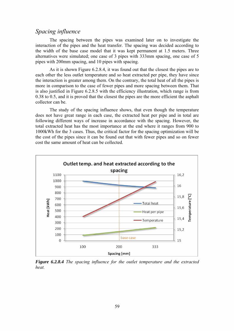
59

Spacing influence The spacing between the pipes was examined later on to investigate the interaction of the pipes and the heat transfer. The spacing was decided according to the width of the base case model that it was kept permanent at 1.5 meters. Three alternatives were simulated; one case of 3 pipes with 333mm spacing, one case of 5 pipes with 200mm spacing, and 10 pipes with spacing.

As it is shown Figure 6.2.8.4, it was found out that the closest the pipes are to each other the less outlet temperature and so heat extracted per pipe, they have since the interaction is greater among them. On the contrary, the total heat of all the pipes is more in comparison to the case of fewer pipes and more spacing between them. That is also justified in Figure 6.2.8.5 with the efficiency illustration, which range is from 0.38 to 0.5, and it is proved that the closest the pipes are the more efficient the asphalt collector can be.

The study of the spacing influence shows, that even though the temperature does not have great range in each case, the extracted heat per pipe and in total are following different ways of increase in accordance with the spacing. However, the total extracted heat has the most importance at the end where it ranges from 900 to 1000kWh for the 3 cases. Thus, the critical factor for the spacing optimization will be the cost of the pipes since it can be found out that with fewer pipes and so on fewer cost the same amount of heat can be collected.

Figure 6.2.8.4 The spacing influence for the outlet temperature and the extracted heat.

60

Figure 6.2.8.5 The spacing influence for the efficiency of the asphalt solar collector.

Depth influence The same three cases like the ones for the spacing influence were used for the investigation of the placement of the pipes under the surface and the examined depths being 50mm, 100mm and 200m.

As it was expected, the fewer the depth from the asphalt surface is the less the outlet temperature and so on the heat per pipe and the total heat extracted from the solar collector is. As it is shown in Figure 6.2.8.6, the outlet temperature ranges from 15 to 16oC for the three cases whereas the total heat ranges from 650 to 1100 kWh. In Figure 6.2.8.7, the efficiency of the three cases in each examined depth is shown and it is indicated that the most efficient spacing and depth is the one of the 3 pipes with 333mm spacing and 50mm depth.

However, the stress concentration on the asphalt occurring from the loading of the parking load should be taken into consideration. In Figure 2.5.6, the Road Energy Systems study has found that stresses are around 0.5MPa in the depth of 50mm and ways of grid support around the pipes and a softer asphalt mix are suggested for the complete safety of the collector. The efficiency then can reach a value of 0.9.

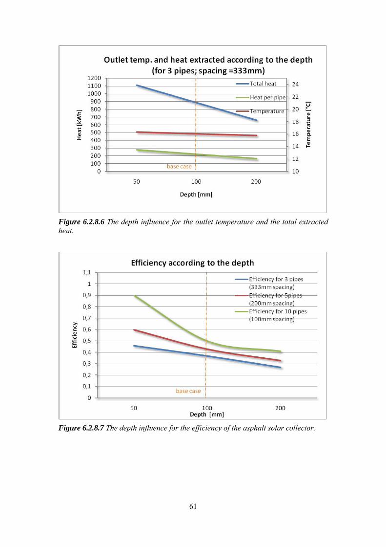
61

Figure 6.2.8.6 The depth influence for the outlet temperature and the total extracted heat.

Figure 6.2.8.7 The depth influence for the efficiency of the asphalt solar collector.

62

Inlet temperature influence The inlet temperature influence was one of the most important parameters to investigate. It is obvious that that the outlet temperature increases when the inlet temperature is higher. On the contrary, the extracted heat, Qextracted, decreases when that happens because of the temperature gradient ΔT, as it is shown in Figure 6.2.8.8. The same effect can be seen in Figure 6.2.8.9 for the efficiency of the solar collector, where the range can vary from 0.7 for low inlet temperatures to 0.25 for higher ones.

However, the decision of the inlet temperature to the piping system is arranged and specified by the temperature of the water mixture that comes from the circulating ground source heat pump system. When the asphalt solar collector is in use during the summer time the temperature and heat produced from the collector is stored in the ground where depending on the ground temperatures and the losses returns a new inlet temperature to the asphalt solar collector. This study is explained later on in the following chapter.

In Figure 6.2.8.10 it is interesting to notice the temperature increase in the outlet temperature when inserting different inlet temperature. As the inlet temperature increases, the temperature gradient decreases. That finds correspondence to the previous Figure 6.2.8.10, where the efficiency has also the same profile to the variable inlet temperatures.

Figure 6.2.8.8 The inlet temperature influence for the outlet temperature and the extracted heat.

63

Figure 6.2.8.9 The inlet temperature influence for the efficiency of the asphalt solar collector.

Figure 6.2.8.10 The temperature increase according to the inlet temperature.

64

Fluid velocity influence The velocity profile of the fluid, u, in m/s, in a pipe can be estimated based on the Reynolds number and the Power Law of Velocity for laminar and turbulent flow according to the following equations [19].

Reynolds number:

Laminar flow :

Turbulent flow

Where

• u is the fluid velocity in m/s,

• ρ is the fluid density in kg/m3 and for the water is 1000 kg/m3

• η is the dynamic viscosity of the fluid in Pa, where for the water is 10-3Pa

• umax is the maximum velocity in m/s, where for safety reasons it should not be more than 2m/s.

• r is radius distance from the center of the pipe in m, and

• R is the diameter of the pipe in m.

All the above can be summed up in Figure 6.2.8.11, where the fluid velocity, u, is plotted against the pipe diameter, R, for the case of a Reynolds number equal to 2300. Over the line turbulent fluid flow takes place, whereas the opposite happens under the line fluid flows correspond to laminar conditions. In the case of the heat transfer, a turbulent flow is more favorable since it is more efficient than the laminar one. In the base case, the fluid with a velocity of 0.1m/s and diameter of 30mm follows a turbulent flow close to the border line, but in many other cases a laminar flow was chosen like in the Worcester Polytechnic Institution research.

After changes in the water velocity, it is visible in Figure 6.2.8.12 that the outlet temperature decreases as the water velocity increases since the fluid is exposed less time to the radiation. The effect of the water velocity seems to be of great importance since the outlet temperature range is from 20 to 15oC. However, the total extracted keeps on increasing and the efficiency in Figure 6.2.8.13 as well.

65

6.2.8.11 The fluid velocity against the pipe diameter in the border line of a turbulent and laminar fluid flow.

Figure 6.2.8.12 The fluid velocity influence for the outlet temperature and the total extracted heat.

66

Figure 6.2.8.13 The fluid velocity influence for the efficiency of the asphalt solar collector.

Pipe diameter with constant water velocity influence In correlation to the water velocity the pipe diameter was also examined. In order to do that firstly a constant water velocity was chosen equal to 0.1 m/s from the base case. In that way the investigation of the pipe diameter influence was easier to be illustrated in Figure 6.2.8.14, where the outlet temperature decreases as the pipe diameter increases, whereas the total extracted heat increases. In Figure 6.2.8.15, the efficiency increases with the pipe diameter especially in the 70mm where it gets even 0.9.

67

Figure 6.2.8.14 The pipe diameter influence for the outlet temperature and the total extracted heat, with a constant water velocity.

Figure 6.2.8.15 The pipe diameter influence for the efficiency of the asphalt solar collector, with a constant water velocity.

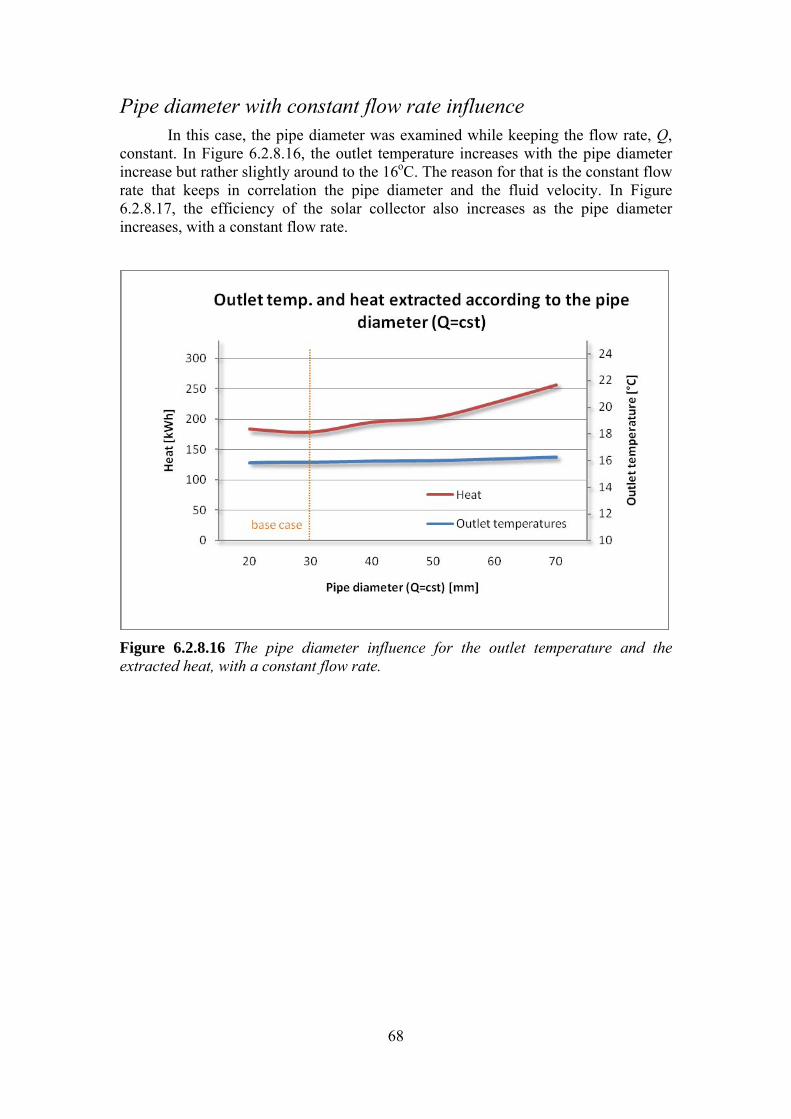
68

Pipe diameter with constant flow rate influence In this case, the pipe diameter was examined while keeping the flow rate, Q, constant. In Figure 6.2.8.16, the outlet temperature increases with the pipe diameter increase but rather slightly around to the 16oC. The reason for that is the constant flow rate that keeps in correlation the pipe diameter and the fluid velocity. In Figure 6.2.8.17, the efficiency of the solar collector also increases as the pipe diameter increases, with a constant flow rate.

Figure 6.2.8.16 The pipe diameter influence for the outlet temperature and the extracted heat, with a constant flow rate.

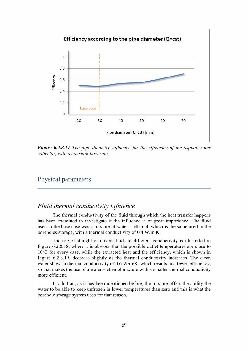
69

Figure 6.2.8.17 The pipe diameter influence for the efficiency of the asphalt solar collector, with a constant flow rate.

Physical parameters

Fluid thermal conductivity influence The thermal conductivity of the fluid through which the heat transfer happens has been examined to investigate if the influence is of great importance. The fluid used in the base case was a mixture of water – ethanol, which is the same used in the boreholes storage, with a thermal conductivity of 0.4 W/m·K.

The use of straight or mixed fluids of different conductivity is illustrated in Figure 6.2.8.18, where it is obvious that the possible outlet temperatures are close to 16oC for every case, while the extracted heat and the efficiency, which is shown in Figure 6.2.8.19, decrease slightly as the thermal conductivity increases. The clean water shows a thermal conductivity of 0.6 W/m·K, which results in a fewer efficiency, so that makes the use of a water – ethanol mixture with a smaller thermal conductivity more efficient.

In addition, as it has been mentioned before, the mixture offers the ability the water to be able to keep unfrozen in lower temperatures than zero and this is what the borehole storage system uses for that reason.

70

6.2.8.18 The fluid thermal conductivity influence for the outlet temperature and the extracted heat.

Figure 6.2.8.19 The fluid thermal conductivity for the efficiency of the asphalt solar collector.

71

Asphalt thermal conductivity influence The investigation of the fluid thermal conductivity influence to the solar collector’s performance was followed by the asphalt thermal conductivity influence. In the base case, the typical asphalt mixture used by NCC was chosen with a thermal conductivity of 1.8 W/m·K.

In Figure 6.2.8.20 it is shown that both the outlet temperature and the extracted heat increase to higher thermal conductivities. In general, the thermal conductivity of the asphalt pavement can be improved with the use of aggregates of higher thermal conductivity, such as quartzite. The same is observed for the efficiency in Figure 6.2.8.21, where the increase of the efficiency rises drastically with the thermal conductivity.

The latest conclusion was also made by the Worcester Polytechnic Institution, where they replaced limestone aggregates with quartzite aggregates to have a 100% temperature gradient in the inlet/outlet water, as it can be seen in Figure 2.4.2.

6.2.8.20 The asphalt thermal conductivity influence for the outlet temperature and the extracted heat.

72

Figure 6.2.8.21 The asphalt thermal conductivity for the efficiency of the asphalt solar collector.

Asphalt surface emissivity influence The emissivity of the asphalt ranges from 0.85 to 0.98, as it was mentioned before. For the base case, the surface asphalt emissivity was assumed to be equal to 0.93, which is given by many handbooks as a typical emissivity value for the asphalt pavements. In Figures 6.2.8.22 and 6.2.8.23, it can be observed that the different emissivity values of that range cannot result in a great difference and all of them lead to an efficiency of around 0.5.

Therefore, the influence of the asphalt surface emissivity cannot be considered to influence the solar collector in a great extent, but only in the case of comparing different materials rather than asphalt.

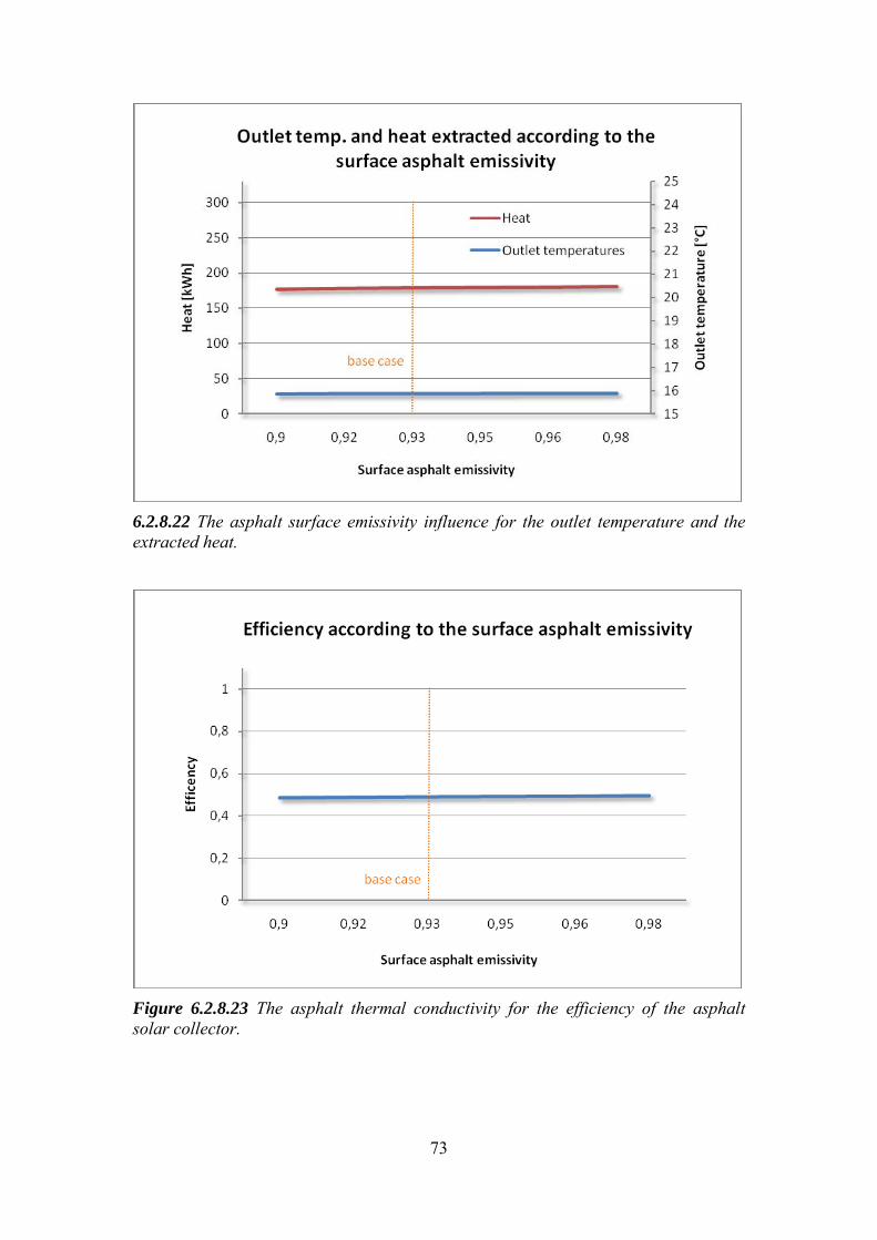
73

6.2.8.22 The asphalt surface emissivity influence for the outlet temperature and the extracted heat.

Figure 6.2.8.23 The asphalt thermal conductivity for the efficiency of the asphalt solar collector.

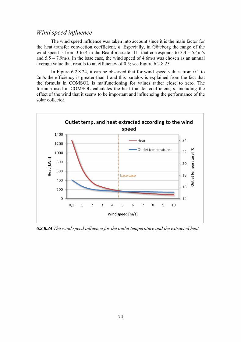
74

Wind speed influence The wind speed influence was taken into account since it is the main factor for the heat transfer convection coefficient, h. Especially, in Göteborg the range of the wind speed is from 3 to 4 in the Beaufort scale [11] that corresponds to 3.4 – 5.4m/s and 5.5 – 7.9m/s. In the base case, the wind speed of 4.6m/s was chosen as an annual average value that results to an efficiency of 0.5; see Figure 6.2.8.25.

In Figure 6.2.8.24, it can be observed that for wind speed values from 0.1 to 2m/s the efficiency is greater than 1 and this paradox is explained from the fact that the formula in COMSOL is malfunctioning for values rather close to zero. The formula used in COMSOL calculates the heat transfer coefficient, h, including the effect of the wind that it seems to be important and influencing the performance of the solar collector.

6.2.8.24 The wind speed influence for the outlet temperature and the extracted heat.

75

Figure 6.2.8.25The wind speed for the efficiency of the asphalt solar collector.

6.2.9 Sensitivity analysis of the parameters A sensitivity analysis provides a better knowledge about the influence of each parameter but overall a better feeling about the parameters importance. Previously, the influence of each parameter, taken separately, has been showed and explained. This part deals with the comparison of the different parameters between each others.

The sensitivity analysis is realized as following: For each parameter separately and starting from the base case value, the value is changed several times to obtain from the simulation a sample of results. The range of values for each parameter is chosen by a rational and consistent manner. In other words, the values have to be likely to be built in a real case. But the range is also determined by the couple computing power and software capacity. For instance, in the base case described the diameter cannot be less than 30mm. As a matter of fact, the number of iterations made by the solver is too large and no converging solution comes out. That can be explained by the difference between the orders of magnitude involved: a pipe of diameter 20mm for a length of 10m. It is most likely a limitation in the software or with computing power used or it could possibly need a COMSOL Multiphysics expert consultation.

Extracted heat sensitivity analysis per parameter

Figure 6.2.9.1 summarizes the previously individual study of the parameters. But it is also an overview of the influence of each parameter on the extracted heat by asphalt collector system. The difficulty to compare each parameter resides in the fact that all the units are different, as well as the order of magnitude of the respective

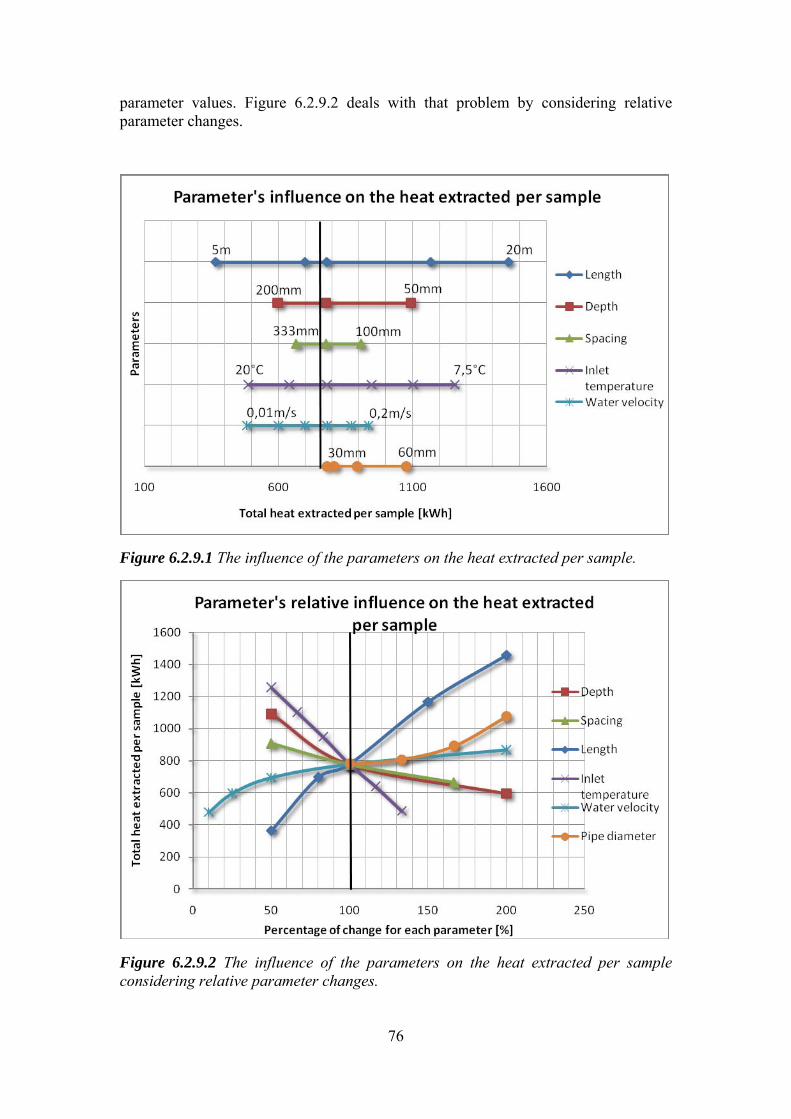
76

parameter values. Figure 6.2.9.2 deals with that problem by considering relative parameter changes.

Figure 6.2.9.1 The influence of the parameters on the heat extracted per sample.

Figure 6.2.9.2 The influence of the parameters on the heat extracted per sample considering relative parameter changes.

77

In Figure 6.2.9.2, it is illustrated the influence of a relative change of a parameter value, in percentage, on the total extracted heat. Even if the percentages of change of values are not completely relevant because of physical constraints, it allows an easier comparison between the parameters. For example, the pipe spacing can be changed largely and very easily compared to the water velocity of the inlet temperatures that are more or less fixed by the outside: the meteorological context and the fluid flows to/from the rest of the system.

In any case, the sensitivity analysis can be done by considering the values of each parameter as they can reasonably be and not taking into account all the constraint the global system; i.e. Ground-source heat pump and borehole seasonal storage, can imply on the asphalt collector.

Pipe depth and Spacing Both depth and spacing are behaving in the same way and with similar intensity. An increase in depth or spacing implies a lesser total heat extraction and vice versa. However, a decrease of the depth seems to be more sensitive than a decrease of spacing. That is because of a closer proximity between the pipe and the surface, which is the source of the conduction heat transfer. As a matter of fact, the surface is a lot warmer than in following depth. The temperature profile is dropping quickly with the depth and therefore a high influence of the depth especially close to the surface. Figure 6.2.9.3 shows depth temperature profile in the inlet side of the collector. The five inlet boundaries can be seen and the 15°C inlet temperature can be noticed. That figure proves the high temperature gradient existing in the depth and consequently the larger influence of the depth once it goes closer to the surface. As a consequence, the depth influence cannot be considered being linear as the influence of the spacing can be.

Figure 6.2.9.3 The depth temperature profile in the inlet side of the collector.

78

Inlet temperature The inlet temperature is behaving in the same way as the pipe spacing and the depth, but the influence is stronger. The evolution of the heat extracted seems to be linear, as far as the chosen range can tell. However, the maximum asphalt temperature is 28°C, if the fluid does not flow in the pipes; there is no cooling of the asphalt. This fact implies that there would be an equilibrium temperature where no heat will be truly extracted by the collector, since the surface temperature and the water temperature would be very close. After that, with a higher inlet water temperature, the process would be reverted and the collector would act like a heater for the asphalt by releasing heat in the asphalt. Fluid velocity and pipe diameter Compared to the previous parameter, the behavior is opposite; i.e. when the parameters increase relatively, the effect is an increase of the total heat extracted. These two parameters are coupled by the fact relation between the flow rate, the fluid velocity and the pipe surface area. In these simulations, the velocity has been kept constant when increasing the diameter, and so the flow rate was changing in function of the diameter value. In addition, if the absolute value is considered for each parameter, the impact is more or less of the same amplitude than the spacing and the pipe depth. Apart from a very small depth or very small fluid velocity, these parameters are similar if the absolute values are taken. Pipe length The length, which behavior matches the pipe diameter and water velocity, has the largest impact on the total extracted heat. For example, the fact to change the length from 10m to 20m, the heat extracted changes from 775 kWh to 1450 kWh. Whereas all the parameters have a visible impact, the length followed by the water inlet temperature seems to have the largest impact on the extracted heat. However, one has to remember that, during the design process, some parameters have constraints either physical or because of the combination of the collector in the global system. Some parameters, such as the pipe diameter, have also a constraint set by the software/computing power combination. These limitations make the design process difficult to execute. Additionally, when designing the collector, the heat extracted is studied in details but the outlet temperature is also of importance. As a matter of fact, if the purpose is to re-charge a borehole system, the heat send to that system is meaningless if the temperature is not taken into account. The aim is to increase the storage temperature by sending a fluid from the collector to the boreholes at a higher temperature.

79

Outlet temperature sensitivity analysis per parameter

The next part of the sensitivity analysis deals with the influence of the parameters on the outlet temperature. Figure 6.2.9.3 shows the ranges of the parameters considered for the sensitivity analysis. The outlet temperature is investigated this time. From this graph, it is clearly the inlet temperature that has the largest impact. It is obvious because the inlet temperature has, of course, a direct impact on the outlet temperature. The water velocity seems to be the second ranked parameter of importance.

Figure 6.2.9.3The influence of the parameters on the outlet temperature per sample.

Figure 6.2.9.4 shows the relative influence of each parameter on the outlet temperature. As stated previously, the inlet temperature has the largest impact and seems to vary linearly. Let us extend the comparison to the others parameters.

80

Figure 6.2.9.4 The influence of the parameters on the outlet temperature per sample considering relative parameter changes.

Length and spacing Whereas the curves are flat compared the inlet temperature, these parameters behave in a similar manner as the inlet temperature. That is to say, it seems to be linear, and only the slope is lower than the inlet temperature. Fluid velocity, pipe diameter and pipe depth These parameters have an opposite impact on the outlet temperature, but have the same impact amplitude as the length and spacing. However, if the fluid velocity is highly decreased to a point where the fluid is almost steady, the outlet temperature is increasing a lot. That is explained by the fact that the almost steady fluid stays a lot longer in the pipe sample considered and though has more time to allow the heat transfer process. The outlet temperature can be very close to the equilibrium temperature, where the fluid temperature almost matches the asphalt surface temperature. But it is useful to remind that a low water velocity will induce a low Reynolds number and a laminar flow. And that is the reason why a lower heat extraction happens; see Figure 6.2.9.1. As matter of fact, the heat transfer is more effective for the case of turbulent flows.

81

Efficiency sensitivity analysis per parameter

Figure 6.2.9.5 shows the ranges of values given to each parameter and the resulting efficiency of the sample. Each parameter effect on the efficiency is rather logical and was easy to guess before doing the simulation with COMSOL Multiphysics. A lower depth, for instance, would increase the efficiency because of the proximity of the collector’s pipes from the asphalt surface which absorbs the sun’s radiation. The simulation allows quantifying with numerical values the impact of a parameter variation.

It seems that all the parameters have a large impact on the efficiency depending on the range used. Following, Figure 6.2.9.6 illustrates the relative variation to make the comparison easier to do.

An easier way to analyze that graph is to focus only on the upper part, the part where the efficiency is increasing; above 0.43 which is the efficiency of the base case. It has been showed previously that a duality exists for a few parameters between the outlet temperature and the heat extracted variation from a change in the parameter value. However, in every single case the best solution is to increase the efficiency of system regardless the heat extracted or the outlet temperature. As a matter of fact the efficiency defined earlier compare the power available from the solar radiation to the heat power extraction made possible by the collector.

Figure 6.2.9.6 is in fact the previous Figure 6.2.9.5 but it only considers the positive effects of parameter variations. In that way, the results can be described easily.

Figure 6.2.9.5The influence of the parameters on the efficiency per sample.

82

Figure 6.2.9.5 The influence of the parameters on the efficiency per sample considering relative parameter changes.

Figure 6.2.9.6 The positive influence of the parameters on the efficiency per sample considering relative parameter changes.

83

Fluid inlet temperature That parameter has the greatest influence on the efficiency. By decreasing the inlet temperature by 50%, from 15°C to 7.5°C, the efficiency becomes 0.69 instead of 0.43. The change in efficiency is drastic and that parameter will be of first importance when designing the collector, whereas the inlet temperature cannot really be chosen, since the fluid comes from the borehole storage system. Pipe depth and pipe diameter Whereas their variations have opposite impacts, they both have a great influence on the efficiency. By doubling or dividing by two, the efficiency evolves from 0.43 to about 0 respectively. Spacing and water velocity These parameters have a lower impact on the efficiency. Indeed, by doubling the values the efficiency reach about 0.5. Length The length has a complex behavior; it is not strictly increasing or decreasing according to the length. That can be explained by a higher outlet temperature and heat extraction when the length increases, but also a higher heated area; i.e. radiation from the sun. So, when the efficiency is calculated, comparing the power supplied by the sun and the power recovered by the collector, the shape of the efficiency curve can be a complicated.

84

85

7 BOREHOLE STORAGE

This chapter focuses on the Ground Source Heat Pump and more especially on the vertical type. The ground – coupled heat pumps are very interestingly compared to the ground-water or ground – surface type because of a lower land area use and a wider range of applicability. These are the reasons why most of the studies, in the past decades, have been carried out to investigate the Ground Source Heat Pump particularly over the other types. The size and the configuration of the heat exchangers are critical for the economical study but also for the energy performance of the global system. Simulation tools are therefore needed to investigate each case and optimize technically and economically the system.

The main objective of the thermal analysis is to determine the fluid temperature in the U-tubes and the heat pump according to particular conditions and over the years; usually a project life time is about 25 years. The “rule of thumb” has been used for a long time but the designers continue to develop new tools because of the “rule of thumb’s” inability to investigate properly the impact of several parameters.

7.1 Theory 7.1.1 The most typical models

The simulation models are divided into two groups. The first one focuses on the heat conduction outside the borehole to calculate the thermal transport around the ground heat exchanger. The most used models are the Kelvin’s line source, the cylindrical source, the Eskilson’s Model, the finite line-source solution and the short time-step model. [24].These models differ mostly from the assumptions made such as finite/infinite source, line/cylindrical source, analytical/numerical method.

The second one focuses on the heat conduction inside the borehole to calculate the fluid temperature and the system’s performance. A few models have been created to describe that, which are: one-dimensional models, two-dimensional models and quasi-three dimensional models.

86

Table 7.1.1 Comparison of the current models of GHEs [24].

Model Method Thermal interaction between boreholes

Boundary effects

Kelvin’s line source Infinite line source Yes No

Cylindrical source Infinite cylindrical source Yes No

Eskilson’s model Combination of numerical

and analytical Yes Yes

Finite line-source solution Analytical method Yes Yes

Outside borehole

Short time-step model Numerical methods Yes Yes

One-dimension No No

Two-dimension Yes No

Inside borehole

Quasi-three-dimension Yes Yes

The numerical models are more accurate compare to the analytical ones, but the computation time is also much higher. The analytical models are also easier to implement in a design program.

7.1.2 The typical programs The GHE design programs must be reliable on a long-term period considering the heat rejection and extraction. The most commonly used programs are the following ones presented in Table 7.1.2.

87

Table 7.1.2 The most common programs used in the design of GHE [24][25].

Programs Description

The Lund programs

Based on the line-source model (Eskilson’s model), the algorithms generates g-functions which are non-dimensional temperature response factors and are dependent on the depth and the borehole spacing. The user interface is not user friendly apart from EED (Earth Energy Designer), which calculates the fluid temperature according to monthly heating and/or cooling loads. The program offers a database with standard values for the thermal properties of the fluid and the ground. The program makes interpolations (causing computing errors) between known g-function to determine solutions depending on the parameters chosen.

The GLHEPRO program

Similar to Lund-programs, it offers however a database for American users.

The GeoStar program

With almost the same capabilities as the Lund-programs, that program was developed by a research group in China.

Building simulation programs with GHE models

The EnergyPlus program is already popular for the building energy simulations and offers a module for GCHP simulations. The model uses the g-functions from Eskilson’s model.

The GchpCalc program

Also designed to investigate vertical GCHP system, this program uses however a cylindrical source model.

Numerical simulation programs

The most famous numerical simulation code is TRNSYS with the DST-module (duct ground storage model) and it is based on finite difference method.

7.2 EED overview The software that has been used for the interseasonal storage of the extracted heat from the asphalt collector system is EED derived from “Earth Energy Design”. It is a program for borehole heat exchanger design and focuses in the ground source heat pump design and borehole thermal storage.

EED has been an outcome Claesson, Eskilson and Hellström’s studies on dimensioning ground heat systems with vertical earth heat exchangers. Algorithms have been derived from modeling and parameter studies with numerical simulation model resulting in analytical solutions of the heat flow with several combinations for the borehole pattern and geometry; i.e. g – functions. Those g – functions depend on the spacing between the boreholes at the ground surface and the borehole depth. The g – function values obtained from the numerical simulations have been stored in a data file, which is accessed for rapid retrieval of data by EED [3]. Some important

88

features, which the program mentions as restrictions of choices for the design of the ground source heat pumps and the boreholes, are shown in Table 7.1.

Table 7.1 Important program features that are taken into consideration for the design of ground source heat pumps and boreholes.

Important program features

Types of boreholes heat exchangers • Coaxial pipes

• U – pipes, i.e. single, double, triple

Borehole depth 20 – 200 meters

Ration borehole spacing/ borehole depth

Time interval

With: and

α = thermal diffusivity in m2/s

Short – time criterion

E1 = exponential integral

7.3 Modeling

The design of the boreholes has been done in accordance with the asphalt solar collector design and in total to fulfill the energy demands for the heating of the residences in Fågelsten. That means the energy heating demands were set as an outcome from the stored energy in the boreholes with the use of a heat pump of a seasonal performance factor which enhances the extracted heat. In addition, the energy injected from the asphalt solar collector to the borehole had to be on balance with the final pumped energy and also to allow the development of an acceptable fluid temperature in the ground. In that case, there have been a number of trials for the energy balance of the combined systems with the goal of identifying a specific design pattern for both the asphalt solar collector and the borehole system in regards to the building heating demands. The energy balance of the combined system is illustrated in Figure 7.2.

89

Figure 7.2 The energy balance of the combined asphalt collector and ground source heat pump system.

7.4 Design data The design data which need to be defied in EED are grouped in the following main categories:

• Ground properties

• Borehole and piping type design

• Heat carrier fluid properties

• Thermal resistances of each component and their interfaces

• Seasonal performance factors

• The monthly energy values for heating and cooling through the year

• The specific heat extraction

• The fluid temperature in the last year of the interest operation.

Ground properties The input data for the ground properties can either be typed directly in case there are measurements from the area or they can be obtained from a database from EED. The ground properties used in the boreholes design were chosen to have the values for Göteborg from EED database, as they are shown in Table 7.4.1.

90

Table 7.4.1 Ground properties obtained from EED’s database for Göteborg.

Ground Properties Göteborg

Thermal conductivity [w/m·K]

Ground heat capacity [J/m3·K]

Ground surface temperature [oC]

Geothermal heat flux [W/m2]

Borehole design The design of the borehole can be chosen among a variety of alternatives depending on the type and the configuration. The type of the boreholes can have one of the following geometries:

• Single BHE

• BHE – Layout in a straight line

• BHE – Layout in a line in L-shape

• BHE – Layout in two parallel L – shaped lines

• BHE – Layout in a line in U – shape

• BHE – Layout in a line forming an open rectangle

• BHE – Layout in form of a rectangular field

While the configuration of the lines can have as many boreholes as each project needs. The rest of the design data can be seen in Table 7.4.2.

For the case of that study two main configurations for of 1x4 and 3x3 of common single U – pipe type have been chosen so as to examine the influence of the configuration to the interseasonal storage. From the literature review, it has been suggested that for the extraction of geothermal energy the line configuration is the favorable one, whereas for the storage a more compact and rectangular configuration is preferred.

The depth of each configuration was chosen so as to have a similar total length for both alternatives of about 800 to 900 meters. The spacing between the boreholes was kept constant. For the rest of the design data such as the borehole’s diameter and the pipe’s diameter, thickness and thermal conductivity the values were kept common for both of the main configurations according to standardization.

91

Table 7.4.2 Borehole design data.

Borehole Alternative 1 Alternative 2

Configuration 1x4 3x3

Depth [m] 200 100

Length [m] 800 900

Spacing [m] 10 4

Diameter [mm] 110

U – pipe

Type Single

Diameter [mm] 40

Thickness [mm] 2.3

Thermal conductivity [W/m·K] 0.42

Shank spacing [mm] 65

Filling thermal conductivity [W/m·K] 0.57

Contact resistance pipe – filling [m·K/W]

0.0

Fluid properties The heat carrier fluid can be selected from a database and in the case of that study the water – ethanol mixture was chosen. The thermal properties of the fluid are presented in the following Table 7.4.3, such as the thermal conductivity, the specific heat capacity, the density, the viscosity the freezing point and the flow rate borehole.

92

Table 7.4.3 The heat carrier properties of the borehole mixture.

Heat carrier fluid properties Fluid: water – ethanol mixture

Thermal conductivity [w/m·K] 0.44

Specific heat capacity [J/kg·K] 4250

Density [kg/m3] 960

Viscosity [kg/ms] 0.0076

Freezing point [oC] -15.0

Flow rate per borehole [l/s] 1.00

Borehole thermal resistance The thermal resistance in a borehole can be either stated, if there are known values from a thermal response test, or they can be calculated each time. The calculation uses an analytical solution that gives an exact solution of the two-dimensional heat conduction problem in a plane transverse to the boreholes axis [18]. The consideration of heat transfer between the individual pipes with the flow up or down is taken into account. The calculated thermal resistances of each component and interface in the borehole for the case of that study are show in Table 7.4.4.

Table 7.4.4 Calculated thermal resistances.

Thermal resistances

Borehole thermal resistance internal [m·K/W] 0.4715

Reynolds number 4021

Thermal resistance fluid – pipe [m·K/W] 0.0011

Thermal resistance pipe material [m·K/W] 0.0463

Contact resistance pipe – filling [m·K/W] 0.0000

Borehole thermal resistance fluid – ground [m·K/W]

0.1103

Effective borehole thermal resistance [m·K/W] 0.1103

93

Seasonal performance factor The seasonal performance factor can be used as an average value for the whole year. Three factors can be introduced and these are for the domestic hot water, the heating and the cooling. In EED for the case of a pump out of operation, that is called “direct cooling”, the SPF is simulated with a large value. The chosen values for that study are shown in Table 7.4.5.

Table 7.4.5 Seasonal Performance factors of the heat pump.

Seasonal Performance factor

Domestic Hot Water [DHW] 3.0

Heating 3.0

Cooling 99999.0

Base loading The monthly energy values for the heating load are introduced according to the energy demands for the Fågelsten case. The cooling load in the ground source heat pump is the injected energy from the asphalt solar collector to the boreholes. In fact the asphalt pavement is cooled down since the heat from its domain is transferred to the ground. In that case then, the cooling load should be adjusted for both the asphalt collector and the boreholes with a number of trials. Four cooling load cases were assumed for the possible operation months from April to August. The cooling load 4 is in fact a zero load were the use of the asphalt collector is neglected so as to examine the reaction of the ground to the extracted heat and how the fluid temperature profiles in the borehole vary. The monthly energy values for the base heating load and the four different cases for the cooling load are shown in Table 7.4.6.

In Figure 7.4.1 the heating load versus the four cooling load cases is illustrated showing that the load that can be injected into the borehole can be anyone in regards to energy but the ground source heat pump will be always capable of providing the specific heat load to the buildings. That means that the load itself is not the one to define the design but the developed fluid temperatures in the borehole as it is described in the following figures.

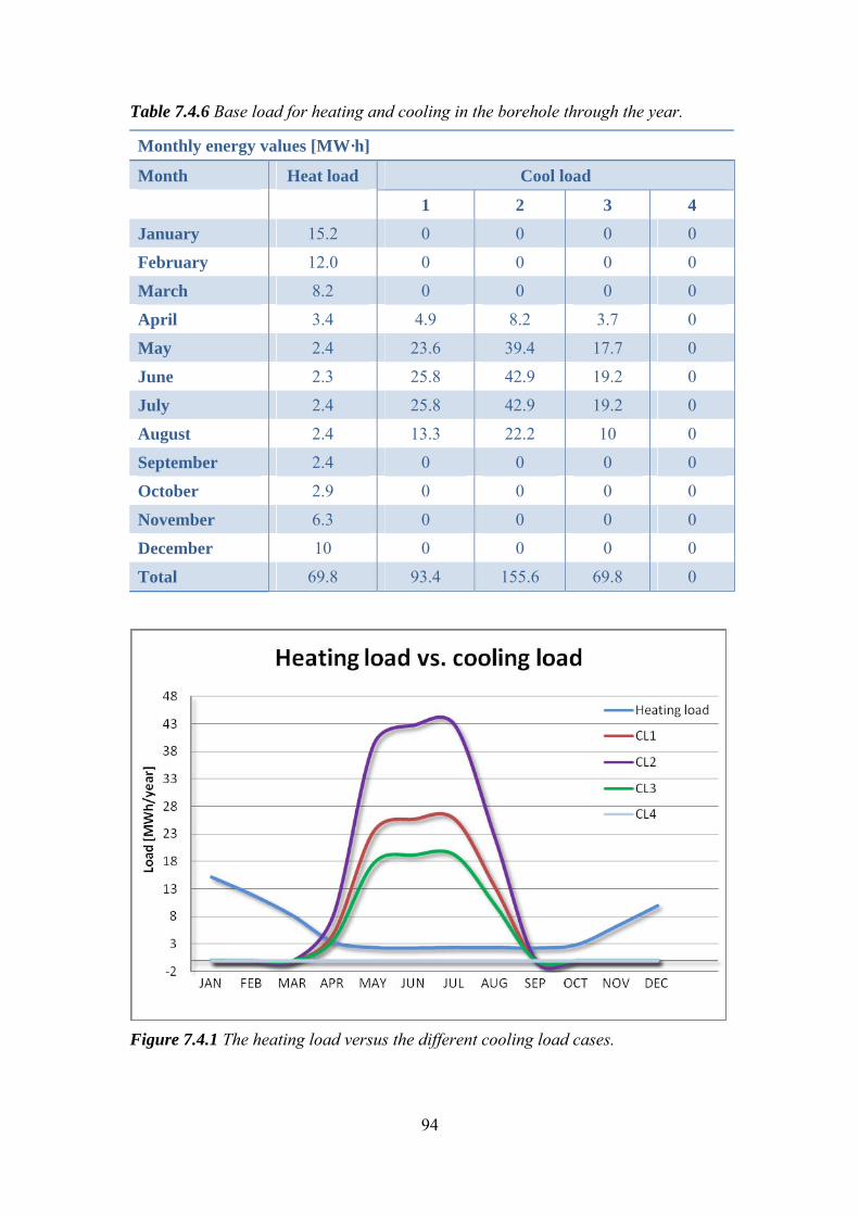
94

Table 7.4.6 Base load for heating and cooling in the borehole through the year.

Monthly energy values [MW·h]

Month Heat load Cool load

1 2 3 4

January 15.2 0 0 0 0

February 12.0 0 0 0 0

March 8.2 0 0 0 0

April 3.4 4.9 8.2 3.7 0

May 2.4 23.6 39.4 17.7 0

June 2.3 25.8 42.9 19.2 0

July 2.4 25.8 42.9 19.2 0

August 2.4 13.3 22.2 10 0

September 2.4 0 0 0 0

October 2.9 0 0 0 0

November 6.3 0 0 0 0

December 10 0 0 0 0

Total 69.8 93.4 155.6 69.8 0

Figure 7.4.1 The heating load versus the different cooling load cases.

95

Borehole fluid developed temperature The life time of the systems operation is set at 25 years and EED can estimate then the mean fluid temperature in that year on a monthly basis. The fluid temperatures for each cooling load case and for the 1x4 borehole configuration is shown in Table 7.4.7, while the illustration of the values is in Figure 7.4.2.

Table 7.4.7 Fluid temperature in the 1x4 borehole configuration for the 25th year of operation.

Fluid temperatures [oC] 1x4 borehole configuration

Month CL1 CL2 CL3 CL4

January 4.30 6.79 3.35 0.56

February 5.23 7.65 4.32 1.61

March 6.52 8.86 5.64 3.02

April 11.13 15.31 9.58 4.89

May 22.54 34.01 18.24 5.38

June 24.58 37.23 19.71 5.51

July 25.08 38.05 20.09 5.53

August 18.23 26.69 15.06 5.57

September 10.48 13.71 9.26 5.64

October 9.83 12.75 8.72 5.45

November 8.26 10.99 7.22 4.15

December 6.58 9.19 5.59 2.66

According to Figure 7.4.2, cooling load cases 1 and 2 can adjust more to the developed outlet temperatures from the asphalt solar collector, when the maximum temperatures correspondingly are 25.08 to 20.09oC are reached during the summer months. In fact, from Figure 6.2.9.4 the sensitivity analysis indicates as potential maximum outlet temperature around 20 to 25oC with the adjustment of different parameters. Cooling load case 2 is resulting to outlet temperatures that in correlation to the asphalt solar collector will give a low efficiency. In comparison to cooling load case 4, which corresponds to no cooling load at all, cooling load cases 1 and 2 will have a maximum temperature difference of 15 to 20oC that is the heat injection from the asphalt collector to the borehole. From this point of view, cooling load case 1 is chosen as the one more close to the reality and the asphalt collector’s function standards.

The fluid temperatures for each cooling load case and for the 3x3 borehole configuration is shown in Table 7.4.8, while the illustration of the values is in Figure 7.4.3.

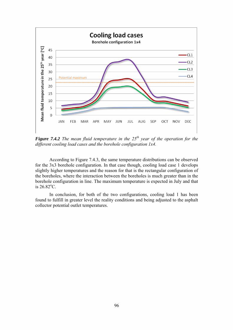
96

Figure 7.4.2 The mean fluid temperature in the 25th year of the operation for the different cooling load cases and the borehole configuration 1x4.

According to Figure 7.4.3, the same temperature distributions can be observed for the 3x3 borehole configuration. In that case though, cooling load case 1 develops slightly higher temperatures and the reason for that is the rectangular configuration of the boreholes, where the interaction between the boreholes is much greater than in the borehole configuration in line. The maximum temperature is expected in July and that is 26.82oC.

In conclusion, for both of the two configurations, cooling load 1 has been found to fulfill in greater level the reality conditions and being adjusted to the asphalt collector potential outlet temperatures.

Potential maximum 

97

Table 7.4.8 Fluid temperature in the 3x3 borehole configuration for the 25th year of operation.

Fluid temperatures [oC] 3x3 borehole configuration

Month CL1 CL2 CL3 CL4

January 6.34 12.04 6.58 0.56

February 6.58 12.00 7.10 1.61

March 7.32 12.44 7.55 3.02

April 11.41 18.11 9.24 4.89

May 22.36 35.98 13.21 5.38

June 25.35 40.71 14.14 5.51

July 26.82 43.07 14.61 5.53

August 21.18 33.65 12.58 5.57

September 13.96 21.49 10.03 5.64

October 12.84 19.68 9.68 5.45

November 10.99 17.38 8.88 4.15

December 8.99 15.02 8.02 2.66

In Figure 7.4.4, there are the fluid temperature curves in the 25th year of operation for cooling load case 1 for the two configurations. It is much easier now to compare and see the differences of the boreholes configuration performance in the interseasonal storage under the same load. From April to May there is no difference in the fluid temperature for both configurations; but in May and later on, when the asphalt solar collector starts to operate, the 3x3 borehole rectangular configuration seems to preserve higher temperature than the 1x4 borehole straight configuration. That conclusion was expected since the rectangular configurations are proved to be more efficient for storage, whereas the straight configuration is preferred for geothermal energy extraction. This can be explained with the excuse that the heat losses from one individual borehole can interact with the other surrounding boreholes in the rectangular configuration.

98

Figure 7.4.3 The mean fluid temperature in the 25th year of the operation for the different cooling load cases and the borehole configuration 3x3.

Figure 7.4.4 The mean fluid temperature in the 25th year of the operation for the cooling load case 1 and the two different borehole configurations 1x4 and 3x3.

99

8 GLOBAL SYSTEM DESIGN In this chapter, the aim is to make the combination of the different systems involved possible. In other words, the building, the seasonal borehole storage and the asphalt solar collector have to be connected and work altogether. The interaction building-heat pump-borehole is made by EED, whereas COMSOL calculates the heat extracted as well as the outlet temperature from the collector. Since the softwares used are completely separated, the link between them is difficult to setup. And that is what this chapter is about, to find a working configuration which matches all the systems involved. Two simple and basic configurations were investigated in that study and are explained in Table 8.1.

Table 8.1 The configuration designs for the piping system of the asphalt collector.

Configuration Description

In parallel One main pipe coming from the borehole circuit feeds x pipes in parallel. Thus, the flow rate in these pipes is the borehole flow rate divided by x. The outlet is one main pipe which collects the fluid from all the pipes in parallel and comes back to the borehole system. See Figure 8.1.

In series One pipe, serpentine-shaped covers the wanted area. In that case, the flow rate is the same everywhere in the circuit. See Figure 8.2.

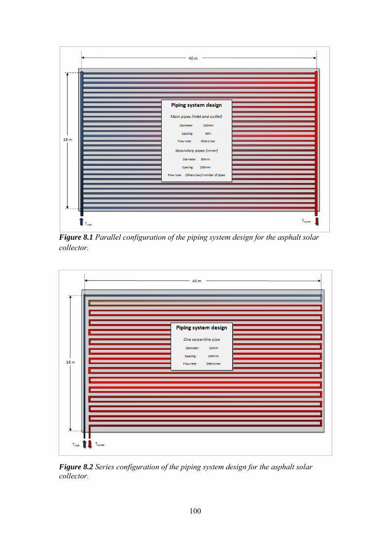
100

Figure 8.1 Parallel configuration of the piping system design for the asphalt solar collector.

Figure 8.2 Series configuration of the piping system design for the asphalt solar collector.

101

In order to work, the system has to meet several design targets such as:

• A flow rate match.

• A maximum fluid velocity of 1.5 – 2m/s to avoid the breaking of the pipes.

• A minimum Reynolds number of 2300 to assure a turbulent flow at any point in the circuit.

Since this investigation is a pre-study, the pressure drops and the pipe resistance are not studied. But it should be kept in mind that the mechanical stresses are neglected, and that should be in the scope of a further study on that system. The investigation has been focused on EED as the center of the system, since the software uses a database about standard sizes and parameters currently used. The idea is to design the asphalt collector by finding a reasonable match with the borehole storage system, whose design is normalized and well-known.

As explained before, the borehole configuration chosen is the rectangular one 3x3. The total flow rate is selected by connecting three times three boreholes in series and then connecting the three subsystems in parallel. Knowing that the flow rate per borehole is 1l/s, which is a common value in EED, the total flow rate is 3l/s.

An Excel file has been created especially to calculate rapidly both Reynolds number flow rate and fluid velocity according to the configuration shape, the number of pipes and different pipe diameters involved. These calculations are shown in Annex II and the following conclusions have been made for the parallel and the series configurations.

Use of COMSOL Due to a lack of computing power and very high simulation time, the models used in COMSOL were only samples of five pipes, starting with the base case defined previously and optimize to match the various parameters needed. To obtain the results for the global design, the results of the different sample were added, for the parallel case, or the output of one sample was the input for the following sample, for the series case. This can cause some uncertainties and approximations in the final results. That was the easiest way to simulate the global system with the tools available for this thesis.

The results could be better if we would have simulated the whole system in COMSOL or another software such as TRNSYS, so that the matching, between the softwares, doesn’t exist. But that wasn’t really feasible in such a short period of time.

102

Parallel configuration After an investigation, it can be concluded that the parallel configuration cannot fulfill the turbulence requirement. As a matter of fact, the flow rate is chosen in EED to generate a turbulent flow for a given borehole diameter. It means that the flow is turbulent but close to become laminar if the velocity or the flow rate is modified. A turbulent flow is needed to keep an efficient heat transfer all the time.

So for a parallel configuration, the flow rate has to be decreased by two orders of magnitude, because about one hundred pipes are needed to meet the heat load of the buildings. In that case, it is not possible to meet both velocity and Reynolds requirement by using realistic pipe diameter. The flow rate of the borehole has to be highly increased. However, this is out of question since the standard values are wanted in the borehole storage. In other words, the flow rate cannot be multiplied by one hundred and stay in a standard borehole design at the same time. Therefore, the configuration in series has been studied after noticing the inability of the parallel configuration to meet all the requirements.

Series configuration This serpentine shape, also called in series, has a range of working diameter that meets both velocity and Reynolds number requirements: from 50mm to 200mm in diameter. The velocity limit is reached by the smallest diameter whereas the Reynolds limitation is reached by the highest diameter.

Even if the highest diameter seems to be more efficient, a 50mm diameter has been chosen in order to limit the pipe costs and the digging and installation costs. In addition, the smallest diameter will save some space, which can be important in some cases. Thus, considering that diameter, the velocity in the pipe is 1.53 m/s.

This configuration has been simulated in COMSOL by adding up the results different samples. The aim was to match as close as possible the temperature profile and the cooling load from EED with the asphalt collector output from COMSOL. As mentioned previously, the heat extraction from the asphalt collector is simulated by EED as a cooling load. In fact, the asphalt is cooled down by the flowing fluid which collects heat to charge the boreholes.

It should be mentioned here that the pressure drops through the pipes have not been checked. That means that, whereas it could be possible to neglect them for the parallel configuration, it is absolutely not the case for the configuration in series. The pressure drops involved are very important and should be studied cautiously in a further study.

The configuration in series will be further investigated in this chapter because it is the best solution from a heat transfer point of view. But if the mechanical and fluid dynamics are investigated, the final and real system would be probably a mix of these two configurations. The parallel configuration to limit the pressure drops and

103

the series configuration to keep the fluid turbulent are required. This mix of configuration will probably need a buffer tank to increase the flow rate compared to the borehole. In that case the flow rate can be divided by the parallel configuration by keeping a turbulent flow.

Considering the series configuration only, the design is explained in the following paragraphs. The simulations in COMSOL were done on a monthly basis. The temperature from March was used as an input temperature in COMSOL for April. The resulting temperature from April in the COMSOL simulation was then used as an input for May, and so on. The resulting asphalt collector size is between 70 and 90 pipes of 40m. The spacing between them being 200mm, means that the width is between 15 and 18m. The total area occupied by the collector is between 560 and 720m.

The fluid temperatures of the asphalt collector outlet for the different simulations and the boreholes fluid are illustrated in Figure 8.3 and compared to the boreholes cooling load. In addition, the cooling and heating loads from EED and the COMSOL simulations for the different numbers of pipes are shown in Figure 8.4. As it has been mentioned in paragraph 7.2.1, the critical parameter of the matching between EED and COMSOL is the developed fluid temperature, since the heating demands will always meet the target.

Figure 8.3 The mean fluid temperature in the 25th year of the operation for the cooling load case 1 and the borehole configuration 3x3 compared with the outlet temperature from two asphalt solar collectors consisted from 70 and 90 pipes respectively and simulated by COMSOL Multiphysics.

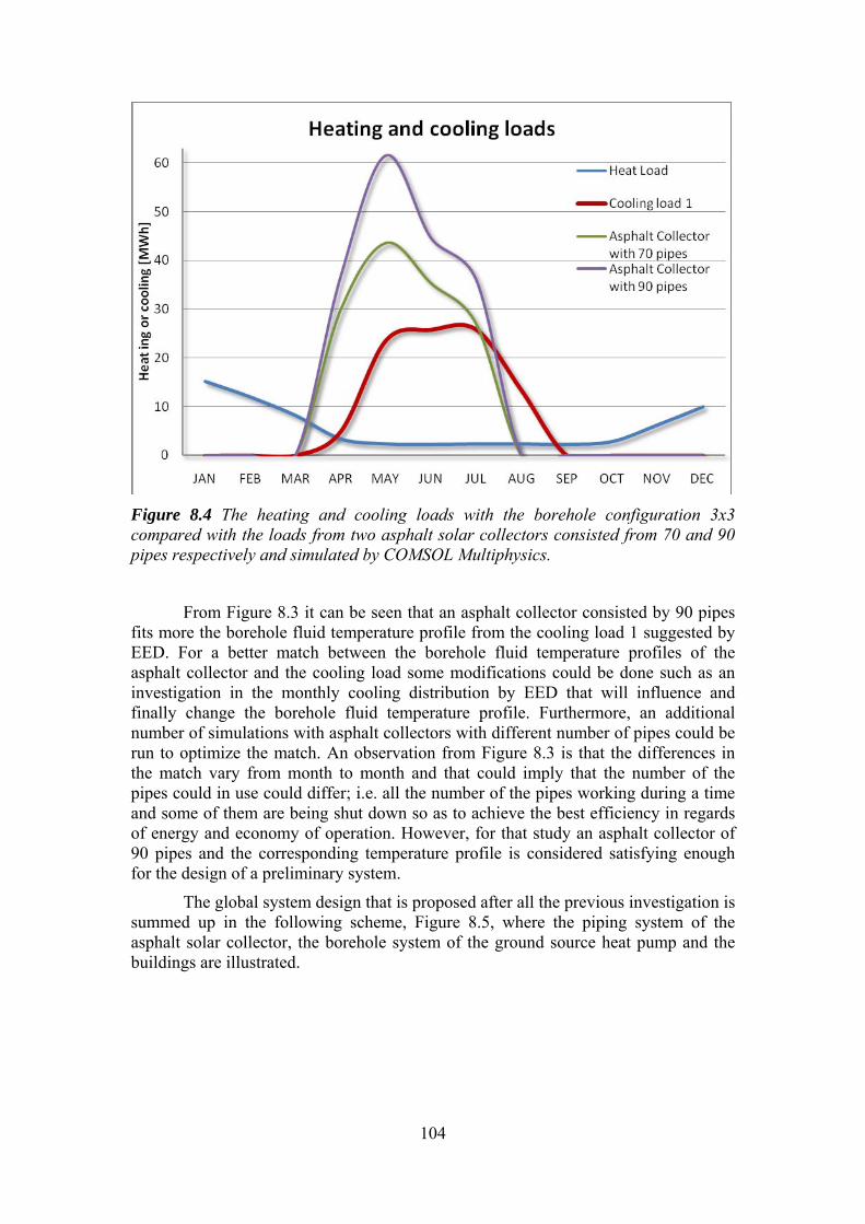
104

Figure 8.4 The heating and cooling loads with the borehole configuration 3x3 compared with the loads from two asphalt solar collectors consisted from 70 and 90 pipes respectively and simulated by COMSOL Multiphysics.

From Figure 8.3 it can be seen that an asphalt collector consisted by 90 pipes fits more the borehole fluid temperature profile from the cooling load 1 suggested by EED. For a better match between the borehole fluid temperature profiles of the asphalt collector and the cooling load some modifications could be done such as an investigation in the monthly cooling distribution by EED that will influence and finally change the borehole fluid temperature profile. Furthermore, an additional number of simulations with asphalt collectors with different number of pipes could be run to optimize the match. An observation from Figure 8.3 is that the differences in the match vary from month to month and that could imply that the number of the pipes could in use could differ; i.e. all the number of the pipes working during a time and some of them are being shut down so as to achieve the best efficiency in regards of energy and economy of operation. However, for that study an asphalt collector of 90 pipes and the corresponding temperature profile is considered satisfying enough for the design of a preliminary system.

The global system design that is proposed after all the previous investigation is summed up in the following scheme, Figure 8.5, where the piping system of the asphalt solar collector, the borehole system of the ground source heat pump and the buildings are illustrated.

105

Figure 8.5 The global system design proposal for Fågelsten case study.

200mm

106

Summing up, the asphalt solar collector design is shown in Table 8.2 and Figure 8.6 and the ground source heat pump in Table 8.3 and Figure 8.7.

Table 8.2 The asphalt solar collector design and performance.

Asphalt Solar Collector

Parameter Value Units

Configuration Serpentine -

Pipe spacing 200 mm

Number of pipes 90 -

Total area occupied 720 m²

Pipe diameter 50 mm

Pipe length 40 m

Total flow rate 3 l/s

Fluid velocity 1.53 m/s

Reynolds number 9650 -

Performance

Period of use April - August

Efficiency Min: 0.28

Max: 0.5

Mean: 0.38

August

May

107

Figure 8.6 The asphalt solar collector design system with the suggested configuration and dimensions of its main components.

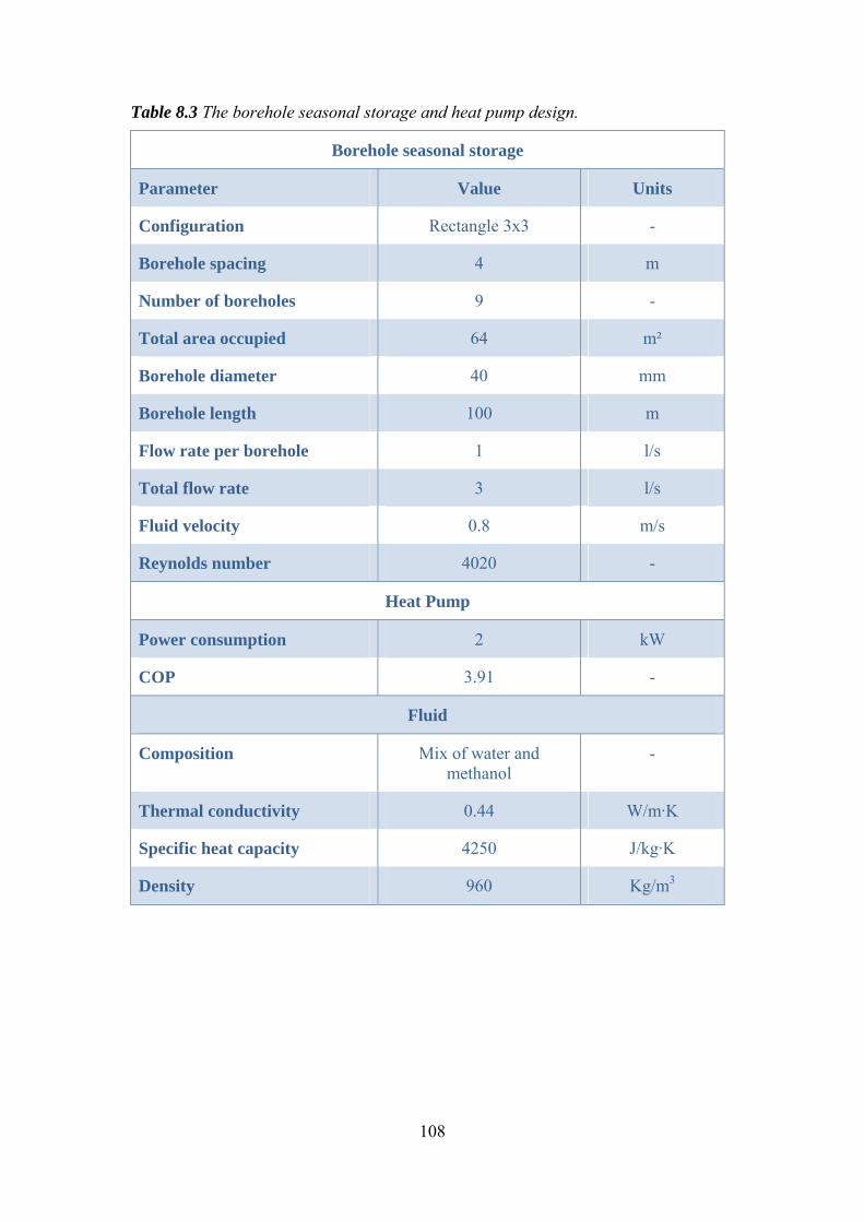
108

Table 8.3 The borehole seasonal storage and heat pump design.

Borehole seasonal storage

Parameter Value Units

Configuration Rectangle 3x3 -

Borehole spacing 4 m

Number of boreholes 9 -

Total area occupied 64 m²

Borehole diameter 40 mm

Borehole length 100 m

Flow rate per borehole 1 l/s

Total flow rate 3 l/s

Fluid velocity 0.8 m/s

Reynolds number 4020 -

Heat Pump

Power consumption 2 kW

COP 3.91 -

Fluid

Composition Mix of water and methanol

-

Thermal conductivity 0.44 W/m·K

Specific heat capacity 4250 J/kg·K

Density 960 Kg/m3

109

Figure 8.7 The borehole design system with the suggested configuration and dimensions of its main components.

110

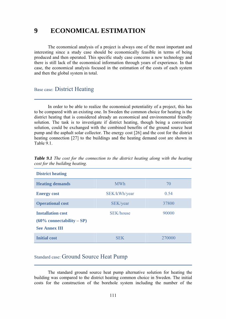
111

9 ECONOMICAL ESTIMATION

The economical analysis of a project is always one of the most important and interesting since a study case should be economically feasible in terms of being produced and then operated. This specific study case concerns a new technology and there is still lack of the economical information through years of experience. In that case, the economical analysis focused in the estimation of the costs of each system and then the global system in total.

Base case: District Heating

In order to be able to realize the economical potentiality of a project, this has to be compared with an existing one. In Sweden the common choice for heating is the district heating that is considered already an economical and environmental friendly solution. The task is to investigate if district heating, though being a convenient solution, could be exchanged with the combined benefits of the ground source heat pump and the asphalt solar collector. The energy cost [26] and the cost for the district heating connection [27] to the buildings and the heating demand cost are shown in Table 9.1.

Table 9.1 The cost for the connection to the district heating along with the heating cost for the building heating.

District heating

Heating demands MWh 70

Energy cost SEK/kWh/year 0.54

Operational cost SEK/year 37800

Installation cost

(60% connectability – SP)

See Annex III

SEK/house 90000

Initial cost SEK 270000

Standard case: Ground Source Heat Pump

The standard ground source heat pump alternative solution for heating the building was compared to the district heating common choice in Sweden. The initial costs for the construction of the borehole system including the number of the

112

boreholes, the depth and the heat pump were researched and then the operational costs that will be constant, as assumed, for every year of the life time of this project. In that case, a borehole configuration of 1x10 was chosen since the boreholes serve for the extraction of heat and not interseasonal storage, as it has been explained in the previous chapter.

A heat pump of 3.38 COP was calculated according to COP expression in paragraph 4.2. A standard ground source heat pump will run with an evaporator temperature close to the average ground temperature. This temperature is 7.5°C for our case study in Lindome. Considering an isentropic efficiency of 0.5 and a standard condenser temperature of 55°C, the COP can calculated as follows:

The expected mean evaporator temperature supplied by the solar collector system is 13°C. This is an increase of 5.5°C of the evaporator temperature.

The new COP is now:

This is considered to be a significant increase of the COP.

The cost can be seen in Table 9.2, while the cumulative cash flow is illustrated in Figure 9.1.

In Figure 9.1, the discount cash flow is taken into consideration, since is a probability in the following years for a discount rate of 4%, as it is suggested by NCC in the economical analysis. In the case when the discount rate is not used the simple payback is 11.5 years, while the discounted payback is 15.7 years. The net present value is 64747 SEK.

113

Table 9.2 The initial construction cost for the ground source heat pump and the operational cost per year.

Ground source heat pump

Quantity of boreholes 1x10 10

Depth of boreholes m 200

Total length m 2000

Drilling and grouting [28] SEK/m SEK 200 400000

Installation [29] SEK 48800

Operating and maintenance [30]

SEK/year 1500

Heat pump energy consumption

MWh 20.71

Electricity cost [31] SEK/kWh SEK/year 1.00 20710.059

COP - 3.38

Figure 9.1 The cumulative cash flow for a standard ground source heat pump.

114

Study case: Asphalt Solar Collector and Ground Source Heat Pump

The asphalt solar collector is introduced in the system so as to decrease the number of the boreholes and also the configuration that in this case will be rectangular and 3x3. The initial cost consists of the pipe cost, the installation and the pump while the operation cost is annual. The ground source heat pump in that case increases the COP from 3.38 to 3.91 because of the increased borehole fluid temperatures developed. The cost for the asphalt collector is shown in Table 9.3 and the cost for the new ground source heat pump is shown in Table 9.4, while the cumulative cash flow is illustrated in Figure 9.2.

Table 9.3 The initial constructional and operational cost for the asphalt solar collector in the global system.

Asphalt Solar Collector

Pipe quantity - 90

Total pipe length m 3200

Area length m 40

Area width m 18

Total area m2 720

Plastic pipes [32] SEK/m SEK 47.2 169920

Installation and paving

SEK/m2 SEK 85 61200

Pump [6] SEK 1545

Supply and installation of the control system

Pump energy consumption

MWh 1.7

Electricity cost [31] SEK/MWh 1000

Operating using electricity

SEK/year 1700

Life time years 25

115

Table 9.4 The initial construction cost for the ground source heat pump and the operational cost per year in the global system.

Ground source heat pump

Quantity of boreholes 3x3 9

Depth of boreholes m 100

Total length m 900

Drilling and grouting [28] SEK/m SEK 200 180000

Installation [29] SEK 48800

Operating and maintenance [30]

SEK/year 1500

Heat pump energy consumption

MWh 17.90

Electricity cost [31] SEK/kWh SEK/year 1.00 17902.81

COP - 3.91

In Figure 9.2, the discount cash flow is taken into consideration in that case as well with the same discount rate of 4%. In the case when the discount rate is not used the simple payback is 11.5 years, while the discounted payback is 15.7 years. The net present value is 69380 SEK.

Figure 9.2 The cumulative cash flow for a standard ground source heat pump with an asphalt solar collector.

116

Systems Comparison

By comparing the two systems, one can say that, even if the initial costs are higher for the second one, the increase of COP from 3.38 to 3.91 generated by the solar collector decreases the electricity costs from the heat pump. In other words, one can afford the second to have higher initial value and still have a lower payback period compared to the district heating. But there is of course a limit to that statement that will be discussed in the next paragraph.

What can be concluded from the cost analysis, is that considering all the cost assumptions above, the GHSP combined with an asphalt solar collector is cheaper than a standard GHSP, only if the installation costs of the collector pipes are less than 85 SEK/m². In addition, if the installation costs become more than 400 SEK/m², the GSHP with asphalt collector has a payback period higher than 25 years compared to the district heating alternative. In the same way, the pipe costs can be investigated in order to see the combinations which make the GSHP with asphalt solar collector more cost-efficient than the standard GSHP. The pipe used as a reference is a plastic pipe for waste water. The price is 47.2 SEK for 3m length and 50mm of diameter.

In Table 9.5 the investigation of the relative initial cash flows by varying the pipe costs and installation costs and keeping the same running costs is shown. When it reaches zero, it means that it reached the maximum possible cash flow that makes the second system as costly as the first, alternatively they have the same payback period that is 11.5 years. The others cells in the table show the cash flow margin or surplus from that reference initial cash flow which is -461465 SEK.

Table 9.5 Relative initial cash flow according to the plastic pipe.

117

Figure 9.3 Cash flow comparisons between a standard GSHP and a GSHP combined with an Asphalt Solar Collector.

Whereas the GSHP combined with an asphalt collector is cost-effective compared to the district heating, it requires a low initial cost to compete against the standard GSHP on a 25 years perspective. A further cost analysis focused on the asphalt collector would be interesting to know make a precise comparison.

Figure 9.4 Lifecycle cost analysis comparing the three alternatives total cost.

118

From a cost point of view, the GSHP combined with an asphalt collector seems cheaper than the standard case if we consider the quantifiable costs involved. However, extra installation costs can appear in the real case and thus make the GSHP with ASC (asphalt solar collector) more costly because of higher initial costs. That can be seen in Figure 9.4. The extra installation costs can change the conclusions of the lifecycle cost analysis totally. In addition, the value of the system can be further enhanced by other advantages or other ways of using that collector. A summary is shown in the following Table 9.6.

Table 9.6 Others advantages and cost reductions when using the GSHP combined with the solar asphalt collector.

Advantages Summer Winter

Asphalt temperature A lower asphalt temperature allows a higher asphalt lifetime.

A higher asphalt temperature allows a higher asphalt lifetime.

Impact on the road A lower car tires degradation.

Ice-free surfaces: no snow truck rounds and no salt needed.

Traffic safety.

The Table 9.6 shows the advantages that can generate savings if the combined system is used and therefore can compete in a better way with the standard GSHP. But these savings are difficult to calculate and an accurate investigation is needed. Plus, the use of the asphalt collector during the winter means that the study has to be restarted from the beginning and new simulations have to done in both COMSOL and EED.

119

10 ENVIRONMENTAL IMPACT

An important part in the design of a new system is the C02 emissions released. Even if most of the design parameters concern the costs and the energy efficiency, the emissions considerations is also a factor to be evaluated in a new project. The determination of the CO2 emissions does not really mean something by itself. It should be compared to a standard case, which is the district heating system in that case.

The estimated CO2 emissions for the district heating in Sweden is 0.075 tCO2/MWh [33], which is energy in terms of heat, while the estimated CO2 emissions for the average electricity in Sweden is 0.090 tCO2/MWh that is in terms of electricity. It has to be mentioned that Göteborg Energi emits less CO2 that the average in Sweden; it is considered to be close to 15 tCO2/MWh [39]. The total heat demand for the building heating of Fågelsten is 70MWh per year. In case there is only the ground source heat pump in use for covering the building heating demands with geothermal energy, then the COP of the heat pump is 3.38, whereas in the case the asphalt solar collector is used the COP of the heat pumps is increased to 3.91. In Table 10.1 the total CO2 emissions are shown of each case of heating system for this study.

Table 10.1 Comparison between the used and suggested heating systems in regards to the environmental impact.

Heating system Emissions

[tCO2/MWh]

Heat demand

[MWh/year]

Total emissions

[tCO2/year]

Savings in comparison to DH

District heating (Sweden average, see Annex III)

0.075

70 5.25 -

District heating (Göteborg Energi)

0.015 70 1.05 -

GSHP 0.090 20.71 1.86 3.39

GSHP & asphalt collector

0.090 19.60 1.76 3.49

In Figure 10 the total emissions of each heating system are illustrated and the savings of the ground source heat pump with and without the asphalt solar collector in comparison to the commonly used districting heating indicate the drastic decrease in the environmental impact with the gas emission decreased approximately 3.5 tons per year. However, it can also be seen in Figure 10 that Göteborg Energi’s district heating saves much more CO2 emissions than all the other systems. It opens a lot of possible discussion about where we should consider the boundaries of the study. Is the goal to

120

be as general as possible to be able to install this system wherever in Sweden, or just consider Göteborg’s case study? Concerning the electricity emissions, they have been taken in average and not on the margin. That can also be discussed: is it new people moving in the flats, or they are coming from another location? In that case, we save electricity elsewhere, and this new use of electricity is not necessarily to be taken on the margin, depending of course of the former heating system and the former electricity use.

Figure 10 The CO2 emissions reductions that can be managed by a ground source heat pump (with or without an asphalt collector) or the district heating in Göteborg compared to the average district heating in Sweden.

The reduction of the CO2 emissions can easily be compared with other emission producing uses as it shown in Table 10.2. So for both the cases of the ground source heat pump with and without an asphalt solar collector different uses with the same emissions are compared. For example, if someone uses a Volvo C30, which emits 151g/km [34], one can cover approximately 22450 km. When using the train to travel from Göteborg to Stockholm, the equivalent trips can be around 8475 considering emissions of 400g per trip [35]. In the case of a longer trip from Göteborg to Bangkok, then the number of the flights is equal to 9 since the emissions during this flight are estimated to be 597 kg [36]. The reduction is also equal to the average CO2 emissions of person in Sweden per year. In order to offset the same amount of carbon dioxide, 32 pine trees are needed [37].

121

Table 10.2 Equivalence of the carbon footprint among different uses.

Equivalence of the CO2 reduction to other emissions

Ground source

heat pump

Ground source heat pump with

asphalt solar collector

CO2 reduction [tCO2/year] 3.39 3.49

Volvo C30 2.0D [km] 22450 23112

GBG-STHLM [trip per person by SJ] 8475 8725

GBG-Bangkok [plane trip by SAS] 5.6 5.9

Pine trees CO2 offset [number] 20.3 20.9

122

123

11 CONCLUSIONS AND DISCUSSION

This Master’s Thesis aimed at evaluating the possibility of using asphalt pavements to capture solar heat during the summer and use seasonal storage in order to recover the heat for heating purposes during the winter.

The asphalt collector model designed in COMSOL Multiphysics allowed getting a better knowledge about the heat extraction, the outlet temperature and the efficiency involved by doing a sensitivity analysis for all the parameters studied. Especially three main parameters, which are the fluid temperature, the pipe diameter and the pipe depth, have strong influence on the efficiency. In order to design collector, the need of obtaining knowledge about borehole storage emerged. EED3 software enabled the design of the asphalt collector considering the specific building heat demand from the study case in Fågelsten.

A global system design has been realized by choosing some values to build a consistent and realistic asphalt collector, whereas some other values were selected to make possible the match a group of parameter to the energy target fixed from the beginning. Thus system is not the most efficient one, but it is made of reasonable chooses during the design. The depth of the pipes is chosen at 200mm, but that value can be reduced and so the efficiency can be enhanced. However, a study in solid mechanics has to be done to determine the stresses and the expected asphalt resistance. Furthermore, a study in fluid dynamics could also be done to analyze the pressure drops generated by the pipe configuration. Even if the configuration has been chosen in that study to satisfy the flow rate from the borehole storage, in reality a mix of both series en parallel configurations combined with a buffer tank is expected to be the most realistic and feasible design.

Taking that global system design, a cost and environmental analysis has been done and the results show a clear benefit for using it compared to the district heating alternative. However, the comparison between this asphalt-solar combined ground source heat pump and a standard ground source heat pump is considered to be uncertain. As a matter of fact, a slight change in the installation costs can be make one system more or less cost-efficient than the other. A further cost study is needed to get more accurate data and have a certain cost estimation and rank properly these two systems. Nevertheless, from an environmental point of view the asphalt-solar combined system is slightly better than the standard case, due to lower the electricity use.

An asphalt solar collector can reveal other economical advantages indirectly or on a long term period. That system can be investigated for heating the road during the winter preventing salt spreading and snow-truck rounds. The road users can benefit from an ice-free way during the winter. That system can also increase the lifetime of the road where it is installed by smoothing the temperature variation during the years.

124

125

REFERENCES

[1] COMSOL Multiphysics 3.5a. “COMSOL Multiphysics - User’s Guide”. November 2008.

[2] COMSOL Multiphysics 3.5a. “Heat Transfer Module - User’s Guide”. November 2008.

[3] EED3.0. “Earth Energy Designer Manual”. May 2008. Available from: http://www.buildingphysics.com/manuals/EED3.pdf [31 May 2010]

[4] Walter J. Eugster. EGEC – Workshop: Geothermal snow melting and de-icing. “Lessons learned in Switzerland”. Malmö, November 2007. Also available information from:

http://www.polydynamics.ch/ [31 May 2010]

[5] D.R. Carder, K.J. Barker, M.G. Hewitt. D Ritter and A. Kiff. “Performance of an interseasonal heat transfer facility for collection, storage and reuse of solar heat from the road surface”. November 2007.

[6] Rajib B. Mallick, Bao-Liang Chen, Sankha Bhowmick. “Reduction of Urban Heat Island Effect through Harvest of Heat Energy from Asphalt Pavements”. “Capturing Solar Energy from Asphalt Pavements”. “A laboratory Study on Reduction of the Heat Island Effect of Asphalt Pavements”. August 2008.

[7] A.H. de Bondt, R. Jansen – Ooms Nederland Holding bv. “Generation and Saving of Energy via Asphalt Pavement Surfaces”. November 2006.

[8] Natural Resources Canada. RETScreen International. “Clean Energy Project Analysis: Engineering & Cases Textbook. Ground – source Heat Pump Project Analysis”. 2005. Available from:

http://www.retscreen.net/ang/textbook_gshp.html [31 May 2010]

[9] Joint Research Center. Available from:

http://re.jrc.ec.europa.eu/pvgis/solres/solrespvgis.htm#Clear-sky [31 May 2010]

[10] RETScreen International Database

[11] Gothenburg climate. Available from:

http://re.jrc.ec.europa.eu/pvgis/solres/solrespvgis.htm#Clear-sky [31 May 2010]

[12] E. Kjellsson. “Solar Collectors Combined with Ground – Source Heat Pumps in Dwellings – Analyses of System Performance”. Lund 2009.

[13] Trafikverket database. Available from:

http://www.trafikverket.se/ [31 May 2010]

[14] Natural Resources Canada. RETScreen International. “Clean Energy Project Analysis: Engineering & Cases Textbook. Solar Water Heating – Project Analysis”. 2005. Available from:

http://www.retscreen.net/ang/textbook_swh.html [31 May 2010]

[15] Natural Resources Canada. “Commercial Earth Energy Systems: A buyer’s Guide”. 2007.

126

[16] Solcomhouse. Available from:

http://www.solcomhouse.com/geothermal.htm [31 May 2010]

[17] Wikipedia. Available from:

http://en.wikipedia.org/wiki/Domestic_energy_consumpontion [31 May 2010]

[18] NCC Fågelsten Brochure. Available from:

http://www.ncc.se/sv/Boende/Sok-Bostad/VastraGotaland/Molndal/Fagelsten/ [31 May 2010]

[19] Bao-Lian Chen Dissertation. “Capture Solar Energy and Reduce Heat – Island Effect from Asphalt Pavement”. December 2008.

[20] COMSOL Multiphysics 3.5a. Heat Transfer Module Database.

[21] Convection – Heat Transfer. Available from:

http://www.engineersedge.com/heat_transfer/convection.htm [31 May 2010]

[22] Wikipedia Natural convection Article. Available from:

http://en.wikipedia.org/wiki/Natural_convection [31 May 2010]

[23] COMSOL Multiphysics 3.5a. “Heat Transfer Module - User’s Guide”. November 2008. Radiation definition.

[24] H. Yang, P. Cui, Z. Fang. Applied Energy “Vertical-borehole ground-coupled heat pumps: a review of models and systems” May 2009

[25] G. Hellström and B. Sanner. “PC-programs and modeling for borehole exchanger design”. 2001

[26] Göteborg Energi. Available from:

http://www.goteborgenergi.se/ [31 May 2010]

[27] R. Nordman. SP, Technical Research Institute of Sweden. “District heating in Sweden”. October 2008.

[28] BorrBoLaget Drilling Company. Available from:

http://www.borrbolaget.se/ [31 May 2010]

[29] Installation costs ??

[30] Heat pump maintenance cost. Available from :

http://pompe-a-chaleur.comprendrechoisir.com/ [31 May 2010]

[31] Electricity prices from Vattenfall. Available from:

http://www.vattenfall.se [31 May 2010]

[32] Plastic waste water pipes. Available from:

http://www.bes.co.uk/products/127.asp#11573 [31 May 2010]

[33] E. Larsson. Swedish District Heating Association “Biomass and district heating in Sweden”. June 2009.

127

[34] CO2 emissions from Volvo cars. Available from:

http://www.volvo.com [31 May 2010]

[35] CO2 emissions from SJ trains. Available from:

http://www.sj.se/sj/jsp/polopoly.jsp?d=260&a=41286&l=en

[36] CO2 emissions from SAS Airlines using the emission calculator available from: http://sasems.port.se/ [31 May 2010]

[37] Erase Carbon Footprint website. Available from:

http://www.erasecarbonfootprint.com/treeoffset.html

[39] Jan-Olof Dalenbäck. Professor in Building Services Engineering.

Chalmers University of Technology - Dept of Energy and Environment

128

129

List of Annexes Annex I: Energy demands for Fågelsten study case

Annex II: Pipe network study in regards to the flow

Annex III: District heating emissions and connection cost

Annex IV: Asphalt recipes from NCC

130

131

ANNEX I: Energy demands for Fågelsten study case

Energy demands of the residential buildings

Preliminary estimations

Summary

The energy calculations for the “Fågelsten Project” result in the following results:

Heated area, house A, B, C 1023 m2

Heated area, storage D 100 m2

Heated area, storage E, F 123 m2

Specific energy demand, house A, B, C 70 kWh/m2 heated area & year

Specific energy demand, store D 83 kWh/m2 heated area & year

Specific energy demand, store E, F 86 kWh/m2 heated area & year

Average U-value for houses A, B, C and stores D, E, F

0,33 W/m2K

The results fulfill the energy standards of the Swedish National Board of Housing.

The energy demands can be influenced in a high degree depending on how the building works, i.e. the tenants’ habits (temperature choice, ventilation, the temperature of the tab warm water etc.). The climate varies among each year, and therefore a year can show higher energy demands. So the results are valid then only for preliminary estimations.

132

ANNEX II: Pipe network study in regards to the flow

133

ANNEX III: District heating emissions and connection cost

Figure 1 The district heating cost connection according to SP Sveriges Tekniska Forskningsinstitut.

Figure 2 Biomass and district heating in Sweden by Henrik Larsson Swedish District Heating Association.

134

ANNEX IV: Asphalt recipes from NCC

135

136

137

Bestämning av glimmerhalt i materialets finfraktion enligt VVMB 613-2001:100                Leverantör / Täkt Karlstad          Produkt Stenmjöl 0-4              Övriga mineral    Glimmer   Kvarts Fältspat   Bergartsfragment Amfibol 0,5-1 mm 1.0%   3.8% 48.1%   47.0% 0.0%         0,250-0,5 mm 2.3%   12.9% 52.3%   32.1% 0.3%       0,125-0,250 mm 7.3%   12.1% 63.2%   15.5% 1.9%      Antal korn   

Analysfraktion (mm)

Biotit Muskovit Amfibol Kvarts Kalifältspat Plagioklas Övriga mineral

Bergartsfragment

Totalt antal korn

0,5-1 3 0   Summa 3 0 11 138 135 287

0,250-0,5 7 0   Summa 7 1 39 158 97 302

0,125-0,250 29 1   Summa 30 8 50 261 64 413