Saving and Preparing School Finance Data from GEMS

Expenditures

Paul Taylor, OPI School Finance

http://opi.mt.gov/Index.html

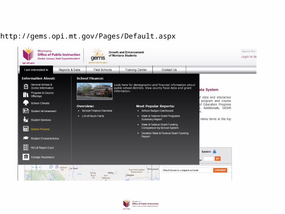
http://gems.opi.mt.gov/Pages/Default.aspx

Choose TFS Reports then Reported Expenditures by School District

Determine your parameters and click View Report

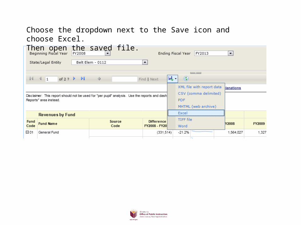
Choose the dropdown next to the Save icon and choose Excel.Then open the saved file.

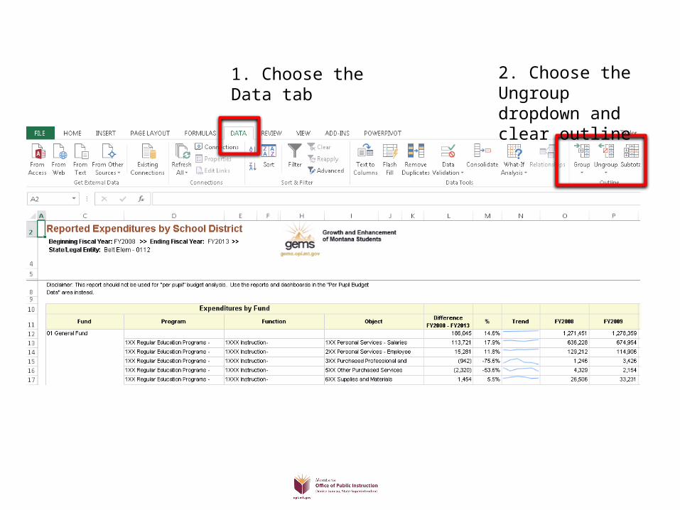
1. Choose the Data tab

2. Choose the Ungroup dropdown and clear outline

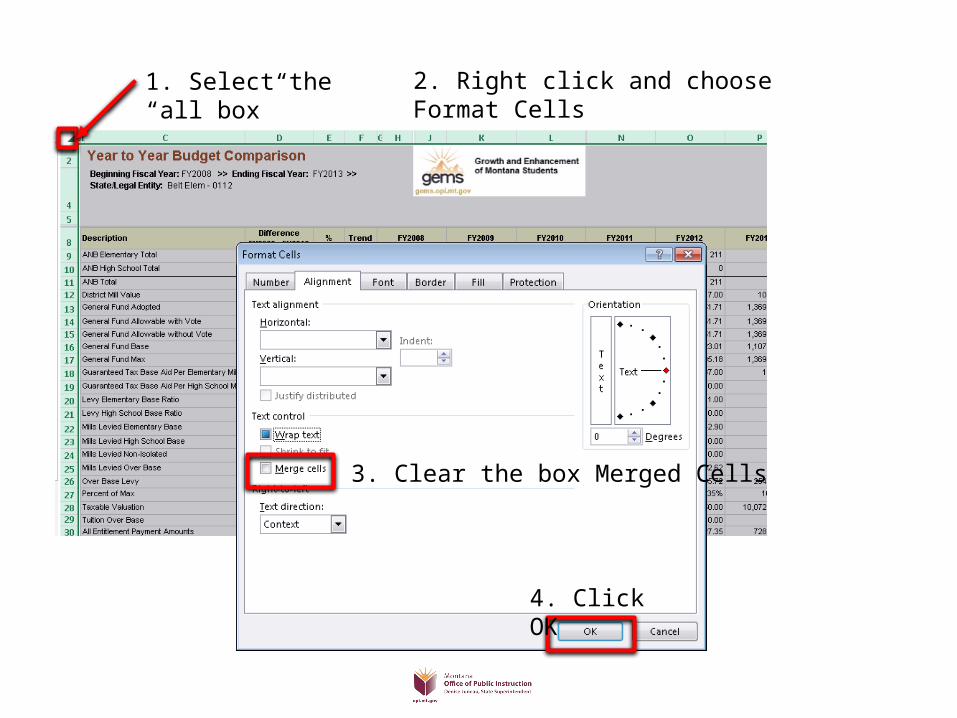
1. Select the “all box” 2. Right click and choose Format Cells

3. Clear the box Merged Cells

4. Click OK

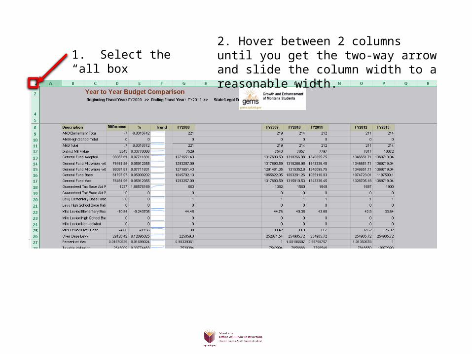
1. Select the “all box”2. Hover between 2 columns until you get the two-way arrow and slide the column width to a reasonable width.

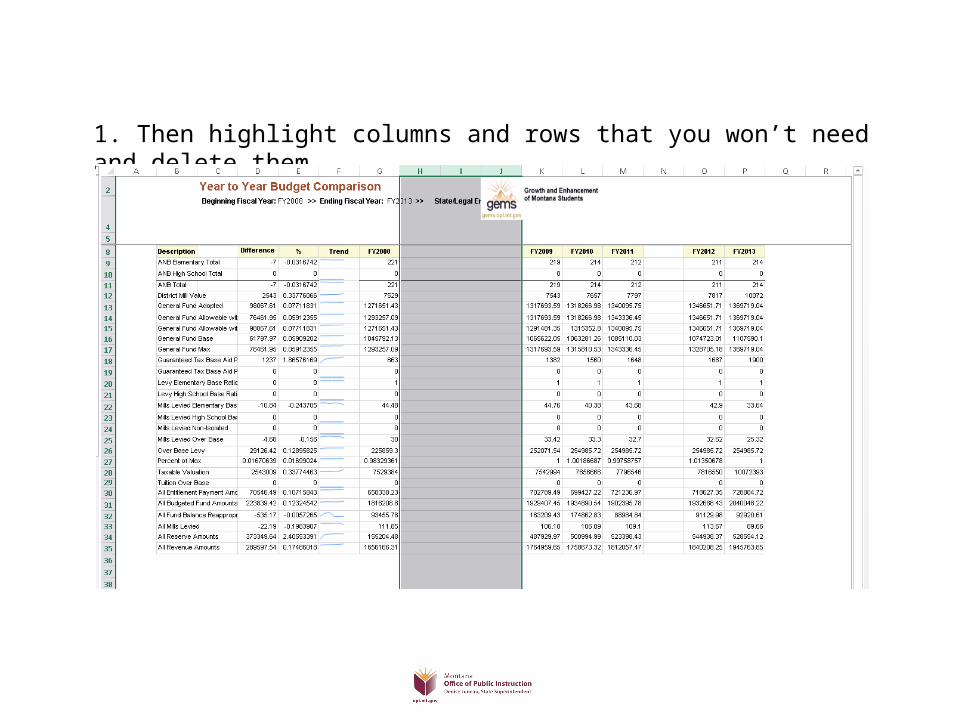
1. Then highlight columns and rows that you won’t need and delete them.

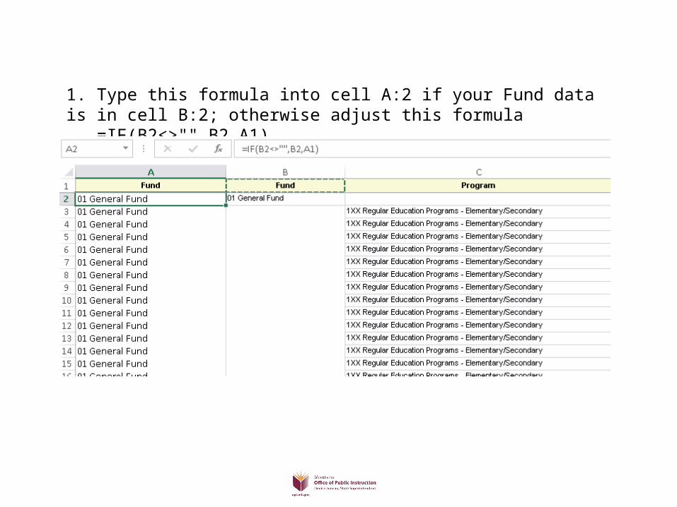
1. Type this formula into cell A:2 if your Fund data is in cell B:2; otherwise adjust this formula =IF(B2<>"",B2,A1)

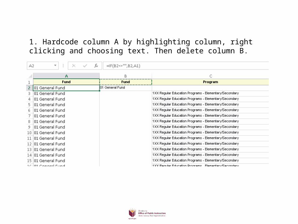
1. Hardcode column A by highlighting column, right clicking and choosing text. Then delete column B.

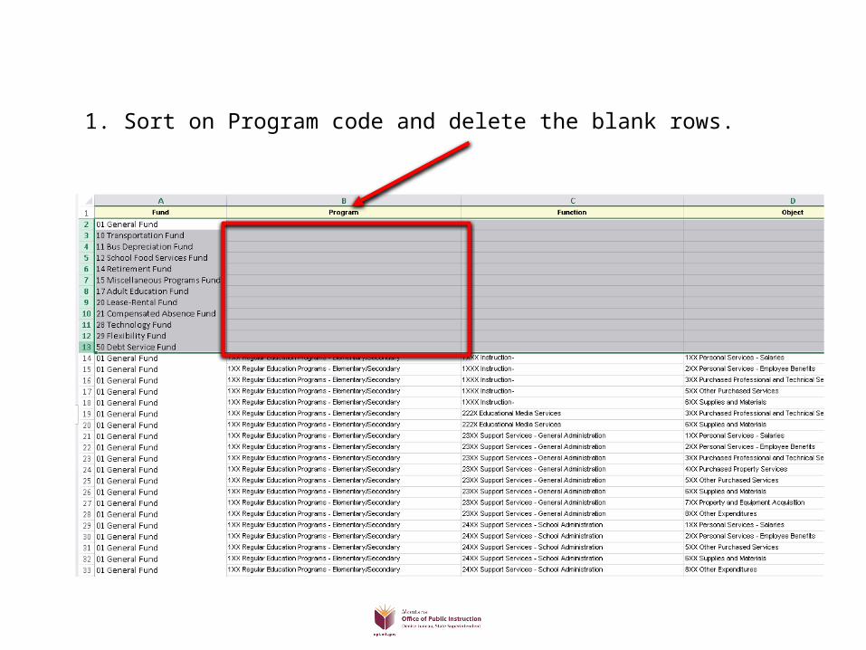
1. Sort on Program code and delete the blank rows.

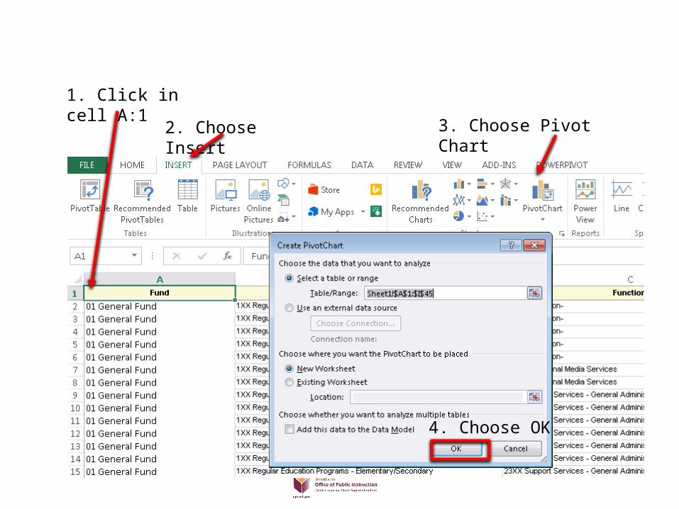
1. Click in cell A:1

2. Choose Insert 3. Choose Pivot Chart

4. Choose OK

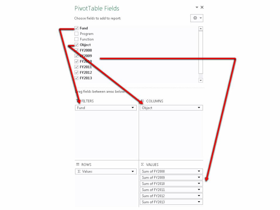
1. Set up your Pivot Table like this by dragging items from the fields area.

A bigger version is on the next slide

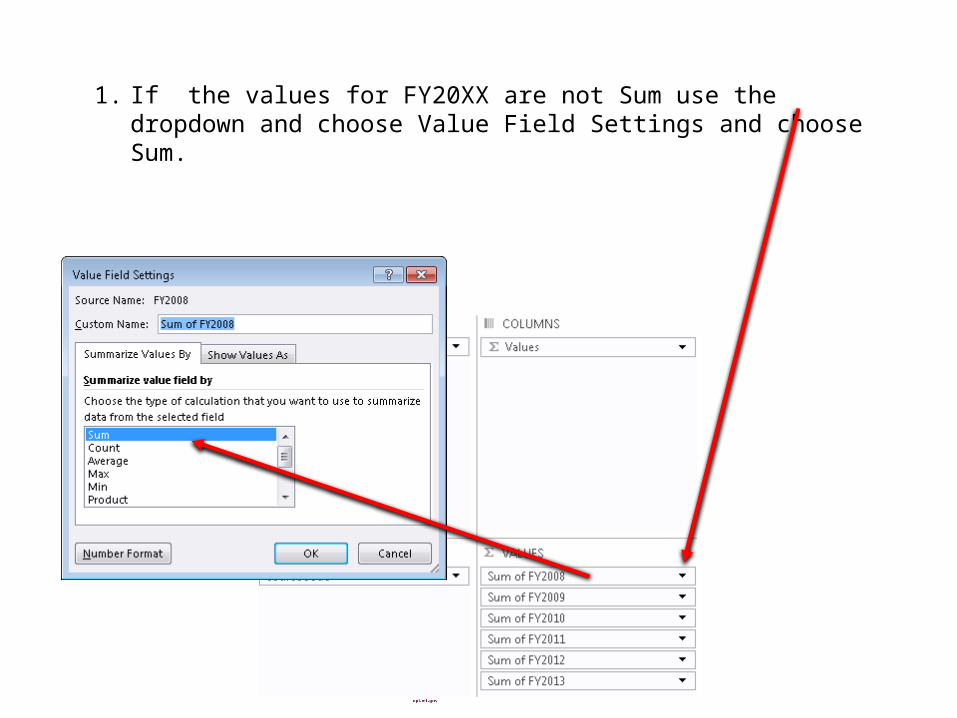
1. If the values for FY20XX are not Sum use the dropdown and choose Value Field Settings and choose Sum.

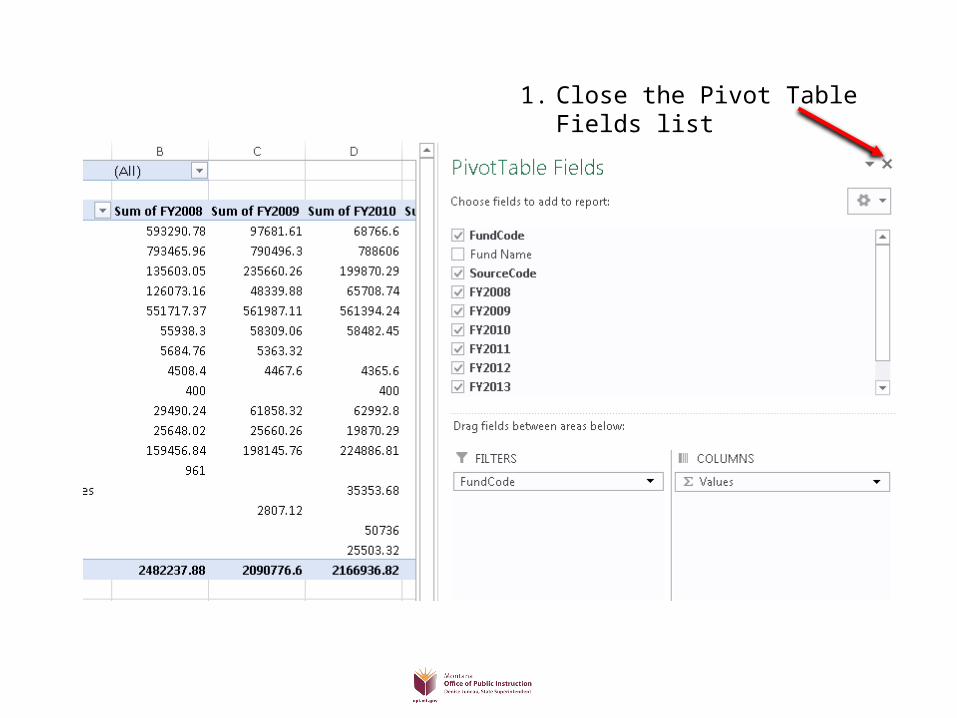
1. Close the Pivot Table Fields list

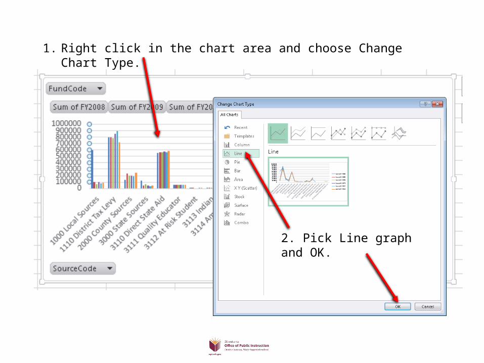
1. Right click in the chart area and choose Change Chart Type.

2. Pick Line graph and OK.

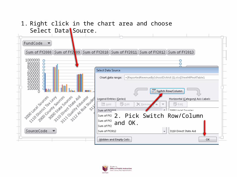
1. Right click in the chart area and choose Select Data Source.

2. Pick Switch Row/Column and OK.

1. Click on the data table.

2. Choose Insert

3. Choose Slicer

4. Choose Fund and Object then OK.

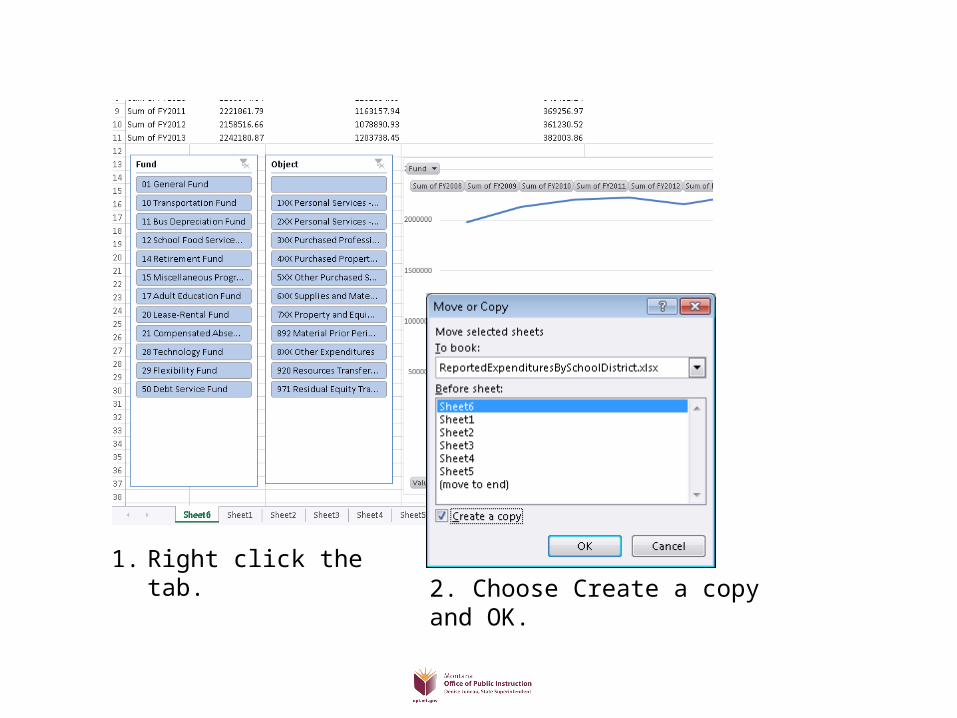
1. Right click the tab.2. Choose Create a copy and OK.

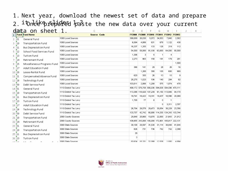
1. Next year, download the newest set of data and prepare it like slides 1-3

2. Once prepared paste the new data over your current data on sheet 1.

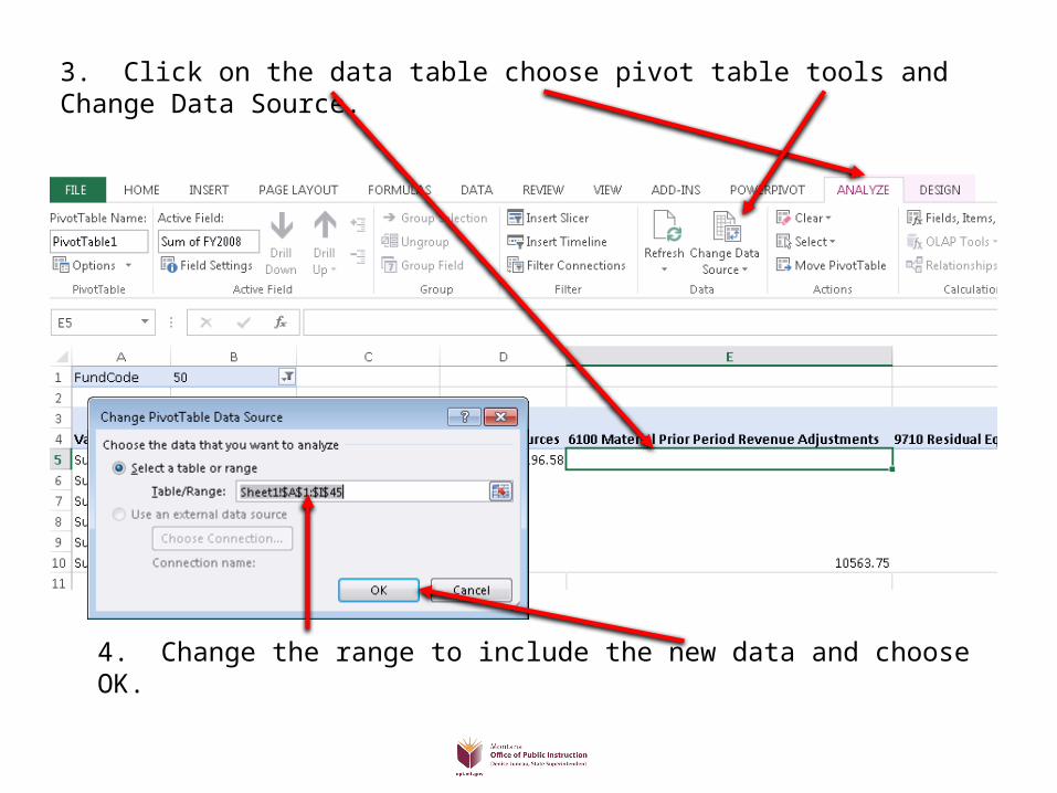
3. Click on the data table choose pivot table tools and Change Data Source.

4. Change the range to include the new data and choose OK.