Embed Size (px)
Citation preview
Saturation temperature effects on heattransfer performance of a falling film
evaporator using enhanced tubes
Master ThesisAndreu Alonso Acuna
Supervisor:Prof. J. R. Thome
January 21, 2011
Abstract
In this work, the existing LTCM falling film facility was utilized to perform
falling film evaporation measurements on a vertical row of horizontal tubes.
The enhanced boiling tube, Wolverine Turbo-B5, was tested using R-134a
and R-236fa. The tests were carried out at different saturation temperatures
of: 7.5◦C, 10◦C, 12.5◦C, 15◦C, 17.5◦C, 20◦C, 22.5◦C, 25◦C, 27.5◦C and 30◦C
adding them to the existing 5◦C saturation temperature in the database
from previous work. All the tests were carried out with liquid film Reynolds
numbers ranging from 0 to 3000, and nominal heat fluxes of 20, 40 and
60 kW/m2. The experimental results for all temperatures are compared
with the current prediction method of Christians (2010). The effects of
the different saturation temperatures on the heat transfer coefficient were
analyzed and compared for R-134a and R-236fa. Pool boiling heat transfer
coefficients were measured in the LTCM pool boiling facility to obtain the
falling film multiplier Kff (Falling film heat transfer coefficient relative to
pool boiling coefficient at the same heat flux). These tests were carried out
at 20◦C and 30◦C for both R-134a and R-236fa. Finally an uncertainty
analysis of the refrigerant film Reynolds number was carried out in order
to quantify the error in its calculation and a new filter for the experimental
data was proposed.

To my family.

Acknowledgements
This work was carried out at the Heat and Mass Transfer Laboratory
(LTCM) at Ecole Polytechnique Federale de Lausanne under the super-
vision of Prof. John R. Thome.
I would like to express my gratitude to all those people who contributed in
different ways to this master thesis, thanks to Prof. John R. Thome for his
support and for supervising this study, to Marcel Christians for his help at
the beginning of this study, to Arturo Gonzalez for all the work that we
did together and his support and finally I would like to express my special
appreciation to Eugene van Rooyen for his help and guidance in the final
and most difficult part of the study.
Furthermore, I would also like to thank my colleagues at the LTCM, who
have created a fantastic work atmosphere and to Cecile Taverney and Nathalie
Matthey-de-L’Endroit for taking care of the administrative work.
Finally, I would like to thank my family for their encouragement and sup-
port.
Contents
1 Introduction 1
2 Literature survey 3
2.1 Introduction . . . . . . . . . . . . . . . . . . . . . . . . . . . . . . . . . . 3
2.2 Falling film mechanics . . . . . . . . . . . . . . . . . . . . . . . . . . . . 3
2.3 Heat transfer mechanisms in falling films . . . . . . . . . . . . . . . . . . 6
2.4 Falling film enhancement . . . . . . . . . . . . . . . . . . . . . . . . . . 6
2.5 Single-array heat transfer studies . . . . . . . . . . . . . . . . . . . . . . 7
2.5.1 Saturation temperature effect . . . . . . . . . . . . . . . . . . . . 8
2.5.2 Layout effect . . . . . . . . . . . . . . . . . . . . . . . . . . . . . 8
2.5.3 Flow rate effect . . . . . . . . . . . . . . . . . . . . . . . . . . . . 8
2.5.4 Heat flux effect . . . . . . . . . . . . . . . . . . . . . . . . . . . . 9
2.5.5 Enhanced surfaces . . . . . . . . . . . . . . . . . . . . . . . . . . 9
2.6 Falling film heat transfer prediction methods . . . . . . . . . . . . . . . 12
2.6.1 Christians (2010) pool boiling prediction method . . . . . . . . . 14
2.6.2 Christians (2010) onset of dryout prediction . . . . . . . . . . . . 16
2.6.3 Plateau heat transfer coefficient prediction method . . . . . . . . 17
2.6.4 Christians (2010) falling film evaporation heat transfer predictions 19
2.6.5 Falling film multiplier . . . . . . . . . . . . . . . . . . . . . . . . 19
2.7 Conclusions . . . . . . . . . . . . . . . . . . . . . . . . . . . . . . . . . . 20
3 Experimental setup 21
3.1 Introduction . . . . . . . . . . . . . . . . . . . . . . . . . . . . . . . . . . 21
3.2 Falling film facility . . . . . . . . . . . . . . . . . . . . . . . . . . . . . . 21
3.2.1 Refrigerant circuit . . . . . . . . . . . . . . . . . . . . . . . . . . 23
iii
CONTENTS
3.2.2 Water circuit . . . . . . . . . . . . . . . . . . . . . . . . . . . . . 25
3.2.3 Test section . . . . . . . . . . . . . . . . . . . . . . . . . . . . . . 27
3.2.3.1 Liquid distribution . . . . . . . . . . . . . . . . . . . . 27
3.2.3.2 Tube layout . . . . . . . . . . . . . . . . . . . . . . . . 30
3.2.4 Measurements procedure . . . . . . . . . . . . . . . . . . . . . . . 31
3.2.4.1 Data acquisition and control . . . . . . . . . . . . . . . 31
3.2.4.2 Measurements and accuracy . . . . . . . . . . . . . . . 32
3.3 Refrigerants . . . . . . . . . . . . . . . . . . . . . . . . . . . . . . . . . . 35
3.4 Data reduction procedure . . . . . . . . . . . . . . . . . . . . . . . . . . 36
4 Experimental Results 39
4.1 Introduction . . . . . . . . . . . . . . . . . . . . . . . . . . . . . . . . . . 39
4.2 Results for R-134a . . . . . . . . . . . . . . . . . . . . . . . . . . . . . . 40
4.3 Results for R-236fa . . . . . . . . . . . . . . . . . . . . . . . . . . . . . 43
4.4 Heat transfer prediction method comparison . . . . . . . . . . . . . . . 47
4.4.1 Prediction vs. Experimental. . . . . . . . . . . . . . . . . . . . . 47
4.4.2 Prediction/Experimental per heat flux . . . . . . . . . . . . . . . 52
4.4.3 Prediction/Experimental per tube type . . . . . . . . . . . . . . 52
4.4.4 Prediction/Experimental per Reynolds number . . . . . . . . . . 55
4.5 Reynolds number uncertainty analysis . . . . . . . . . . . . . . . . . . . 55
4.6 Proposed new experimental data filter . . . . . . . . . . . . . . . . . . . 61
4.6.1 Heat transfer coefficient uncertainty filter . . . . . . . . . . . . 61
4.6.2 New experimental data filter . . . . . . . . . . . . . . . . . . . 61
4.7 Falling film multiplier . . . . . . . . . . . . . . . . . . . . . . . . . . . . 62
4.7.1 Results for R-236fa . . . . . . . . . . . . . . . . . . . . . . . . . 64
4.7.2 Results for R-134a . . . . . . . . . . . . . . . . . . . . . . . . . . 66
5 Conclusion 69
Appendices
A LTCM implementation of the Wilson plot method 71
A.0.3 Heat transfer calculation principles . . . . . . . . . . . . . . . . . 71
A.0.4 Wilson plot method 1915 . . . . . . . . . . . . . . . . . . . . . . 72
A.0.5 LTCM implementation of the Wilson plot method . . . . . . . . 74
iv
CONTENTS
A.0.5.1 Tube-side formulation . . . . . . . . . . . . . . . . . . . 75
A.0.5.2 Shell-side formulation . . . . . . . . . . . . . . . . . . . 75
A.0.5.3 Uncertainty propagation through the linear regression . 76
B Pool boiling facility 77
References 81
v

CONTENTS
vi
List of Figures
2.1 Intertube falling-film mode . . . . . . . . . . . . . . . . . . . . . . . . . 4
2.2 Schematic of liquid film breakdown for two different film flow rates . . . 5
2.3 Schematic of the variation of heat transfer coefficient with flow rate for
falling film evaporation . . . . . . . . . . . . . . . . . . . . . . . . . . . . 9
2.4 Cross-over characteristics of pored enhanced tubes . . . . . . . . . . . . 10
3.1 Schematic of the falling film facility. . . . . . . . . . . . . . . . . . . . . 22
3.2 Schematic of the falling film evaporation refrigerant circuitry . . . . . . . 23
3.3 Schematic of the forced-circulation water-glycol circuit . . . . . . . . . . 25
3.4 Schematic of the forced-circulation loop for the heating water . . . . . . 26
3.5 Schematic of the test section . . . . . . . . . . . . . . . . . . . . . . . . 28
3.6 Schematic of the liquid distributor . . . . . . . . . . . . . . . . . . . . . 29
3.7 Schematic of the tube layout. . . . . . . . . . . . . . . . . . . . . . . . . 30
3.8 Instrumented temperature measurement rod inserted into water side of
tubes . . . . . . . . . . . . . . . . . . . . . . . . . . . . . . . . . . . . . 34
4.1 Heat transfer coefficients vs. Film Reynolds number for 20 kWm−2 for
R-134a . . . . . . . . . . . . . . . . . . . . . . . . . . . . . . . . . . . . . 41
4.2 Heat transfer coefficients vs. Film Reynolds number for 40 kWm−2 for
R-134a . . . . . . . . . . . . . . . . . . . . . . . . . . . . . . . . . . . . . 41
4.3 Heat transfer coefficients vs. Film Reynolds number for 60 kWm−2 for
R-134a . . . . . . . . . . . . . . . . . . . . . . . . . . . . . . . . . . . . . 42
4.4 Heat transfer coefficients vs. Film Reynolds number for 60 kWm−2 for
R-134a and saturation temperatures of 10◦C, 12.5◦C, 25◦C and 30◦C . . 42
vii
LIST OF FIGURES
4.5 R-134a. Heat transfer coefficients vs. Film Reynolds number for the
three nominal heat fluxes for all tubes (a) and the three nominal heat
fluxes on the top three tubes in the array (b) . . . . . . . . . . . . . . . 43
4.6 R-236fa. Heat transfer coefficients vs. Film Reynolds number for 20
kWm−2 . . . . . . . . . . . . . . . . . . . . . . . . . . . . . . . . . . . . 44
4.7 R-236fa. Heat transfer coefficients vs. Film Reynolds number for 40
kWm−2 . . . . . . . . . . . . . . . . . . . . . . . . . . . . . . . . . . . . 45
4.8 R-236fa. Heat transfer coefficients vs. Film Reynolds number for 60
kWm−2 . . . . . . . . . . . . . . . . . . . . . . . . . . . . . . . . . . . . 45
4.9 Heat transfer coefficients vs. Film Reynolds number for 60 kWm−2 for
R-236fa and saturation temperatures of 10◦C, 12.5◦C, 25◦C and 30◦C . 46
4.10 R-236fa. Heat transfer coefficients vs. Film Reynolds number for the
three nominal heat fluxes (a) and Heat transfer coefficients vs. Film
Reynolds number for the three nominal fluxes the top three tubes in the
array (b) . . . . . . . . . . . . . . . . . . . . . . . . . . . . . . . . . . . 46
4.11 R-134a. Prediction vs. Experimental for all the tubes in the array and
for all the data on the plateau and partial dryout . . . . . . . . . . . . . 48
4.12 R-134a. Prediction vs. Experimental with only data in the plateau
region for all the tubes in the array . . . . . . . . . . . . . . . . . . . . . 48
4.13 R-134a. Prediction vs. Experimental for the three top tubes of the array
indicating the correlation for plateau and partial dryout . . . . . . . . . 49
4.14 R-134a. Prediction vs. Experimental with selected data from the plateau
region and the top three tubes of the array only . . . . . . . . . . . . . . 50
4.15 R-236fa. Prediction vs. Experimental for all the tubes in the array and
for all the data on the plateau and partial dryout . . . . . . . . . . . . . 50
4.16 R-236fa. Prediction vs. Experimental with only data in the plateau
region for all the tubes in the array . . . . . . . . . . . . . . . . . . . . . 51
4.17 R-236fa. Prediction vs. Experimental for the three top tubes of the
array indicating the correlation for plateau and partial dryout . . . . . . 51
4.18 R-236fa. Prediction vs. Experimental with selected data from the
plateau region and the top three tubes of the array only . . . . . . . . . 52
4.19 R-134a. Prediction/Experimental fraction as a function of heat flux for
all data (plateau and partial dryout) . . . . . . . . . . . . . . . . . . . . 53
viii
LIST OF FIGURES
4.20 R-236fa. Prediction/Experimental fraction as a function of heat flux for
all data (plateau and partial dryout) . . . . . . . . . . . . . . . . . . . . 53
4.21 R-134a. Prediction/Experimental fraction plotted per tube row . . . . . 54
4.22 R-236fa. Prediction/Experimental fraction plotted per tube row . . . . 54
4.23 R-134a. Prediction/Experimental fraction plotted vs. Reynolds number
and clearly indicating higher accuracy in the plateau region . . . . . . . 55
4.24 R-236fa. Prediction/Experimental fraction plotted vs. Reynolds number
and clearly indicating higher accuracy in the plateau region . . . . . . . 56
4.25 Percentage film Reynolds number uncertainty plotted against film Reynolds
number calculated in the array for R-236fa . . . . . . . . . . . . . . . . 59
4.26 Percentage film Reynolds number uncertainty plotted against tube num-
ber in the array . . . . . . . . . . . . . . . . . . . . . . . . . . . . . . . 59
4.27 R236. Absolute film Reynolds number uncertainty vs. film Reynolds
number on the array for every tube in the array and all experimental
temperatures . . . . . . . . . . . . . . . . . . . . . . . . . . . . . . . . . 60
4.28 R236. Absolute film Reynolds number uncertainty vs. tube row for all
temperatures . . . . . . . . . . . . . . . . . . . . . . . . . . . . . . . . . 60
4.29 Pool boiling heat transfer coefficient vs. heat flux for R-236fa in the pool
boiling facility . . . . . . . . . . . . . . . . . . . . . . . . . . . . . . . . . 63
4.30 Pool boiling heat transfer coefficient vs. heat flux for R-134a in the pool
boiling facility . . . . . . . . . . . . . . . . . . . . . . . . . . . . . . . . . 63
4.31 R236fa. Falling film multiplier vs. film Reynolds number for Tsat = 5◦C 64
4.32 R236fa. Falling film multiplier vs. film Reynolds number for Tsat = 20◦C 65
4.33 R236fa. Falling film multiplier vs. film Reynolds number for Tsat =30◦C 65
4.34 R134a. Falling film multiplier vs. film Reynolds number for Tsat = 5◦C 67
4.35 R134a. Falling film multiplier vs. film Reynolds number for Tsat = 20◦C 67
4.36 R134a. Falling film multiplier vs. film Reynolds number for Tsat =30◦C 68
B.1 Schematic of the pool boiling refrigerant circuit . . . . . . . . . . . . . . 78
B.2 Schematic of the pool boiling water circuit . . . . . . . . . . . . . . . . . 79
ix

LIST OF FIGURES
x
List of Tables
2.1 Geometric factors (Gt−s) for all enhanced tubes included in the database 16
3.1 Experimental test conditions . . . . . . . . . . . . . . . . . . . . . . . . 21
3.2 Properties of R-134a and R-236fa and their relative variation at 5◦C . . 35
4.1 Empirical coefficients for pool boiling on tube Turbo-B5: ho,pb = C · qn . 64
B.1 Experimental test conditions for pool boiling tests . . . . . . . . . . . . 77
xi

LIST OF TABLES
xii
1
Introduction
Large Evaporation units are used in the refrigerant industry. In flooded evaporators,
liquid refrigerant enters the evaporator from the bottom and evaporates as it moves up
the tube bundle due to the difference in buoyancy between the two phases. Falling film
evaporators, on the other hand, are based on a heat transfer process that takes place
when the refrigerant is flowing downwards, due to gravity, onto a heated tube bundle.
When utilized in a refrigeration system, falling film evaporators present several advan-
tages compared to flooded evaporators, particularly in terms of higher cycle efficiency,
reduced costs and smaller environmental impact due to the reduced refrigerant charge
required. Pressure drop is negligible as the liquid flows due to the action of gravity.
However, a re-circulation pump may be required to bring the liquid from the bottom
to the top of the evaporator. Many parameters influence the falling film evaporation
process and, despite numerous studies, the basic mechanisms remain unclear.
The primary objectives of this study were the testing and characterization of the
saturation temperature effects on one enhanced tube using two refrigerants, R-134a and
R-236fa. Due to the low pressure drops observed during the falling film evaporation,
the heat transfer was the most important parameter to study. This new experimental
data was collected to help to better understand the mechanisms dominant in refriger-
ant evaporation. This, in the long run, should allow designers to more-efficiently size
heat exchangers, and make them more economically viable, as well as environmentally
sustainable.
As a result of this experimental campaign, a total of 11,600 data points were gath-
ered and added to the LTCM falling film database which already had about 55,000
1
1. INTRODUCTION
experimental points. Two new saturation temperatures for both R-134a and R-236fa
were measured in the LTCM pool boiling facility to obtain the falling film multiplier
Kff and added to the LTCM pool boiling database.
The study is presented with the following layout: in Chapter 2, a brief summary
of recent falling film and pool boiling studies regarding heat transfer are presented,
as well as a discussion of the factors that affect falling film evaporative heat transfer.
Chapter 3 describes the design, operation and instrumentation of the falling film facility.
Chapter 4 discusses the experimental results on falling film evaporation and pool boiling
evaporation at different saturation temperatures. Appendix A presents the LTCM
implementation of the Wilson plot method. Appendix B describes the design of the
pool boiling facility.
2
2
Literature survey
2.1 Introduction
Falling film evaporative heat transfer is affected by several primary factors. A brief
summary of recent falling film and pool boiling studies regarding heat transfer is pre-
sented, as well as a discussion of the factors that affect falling film evaporative heat
transfer.
2.2 Falling film mechanics
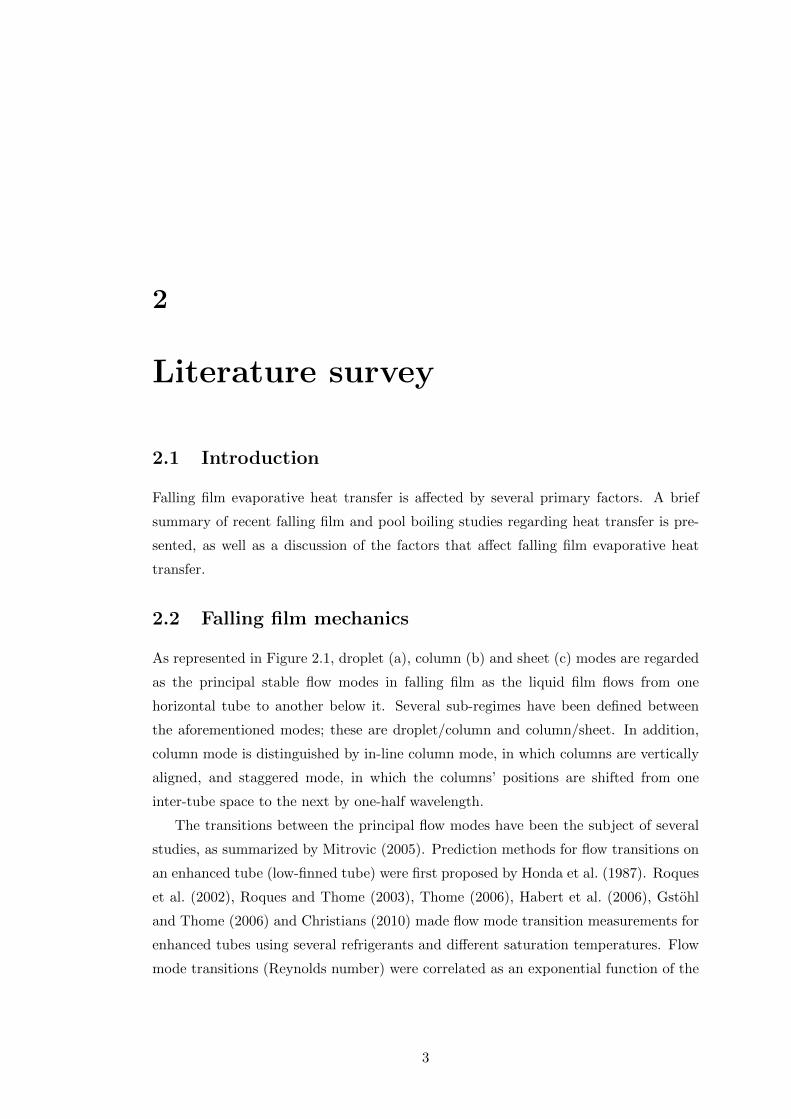
As represented in Figure 2.1, droplet (a), column (b) and sheet (c) modes are regarded
as the principal stable flow modes in falling film as the liquid film flows from one
horizontal tube to another below it. Several sub-regimes have been defined between
the aforementioned modes; these are droplet/column and column/sheet. In addition,
column mode is distinguished by in-line column mode, in which columns are vertically
aligned, and staggered mode, in which the columns’ positions are shifted from one
inter-tube space to the next by one-half wavelength.
The transitions between the principal flow modes have been the subject of several
studies, as summarized by Mitrovic (2005). Prediction methods for flow transitions on
an enhanced tube (low-finned tube) were first proposed by Honda et al. (1987). Roques
et al. (2002), Roques and Thome (2003), Thome (2006), Habert et al. (2006), Gstohl
and Thome (2006) and Christians (2010) made flow mode transition measurements for
enhanced tubes using several refrigerants and different saturation temperatures. Flow
mode transitions (Reynolds number) were correlated as an exponential function of the
3
2. LITERATURE SURVEY
Figure 2.1: Intertube falling-film mode -
Galileo number (Re = aGab). Ribatski and Jacobi (2005) compared the then-available
prediction methods for flow mode transitions and found significant scatter among them.
This was expected, due to the subjective nature of visually interpreting two-phase flow
regime transitions. The correct design of falling film heat exchangers such that the flow
mode is optimal is an important parameter to consider. For falling film evaporation,
sheet mode seems to be the most convenient as this mode should best avoid formation
of dry patches on the tubes.
Film breakdown occurs when the flow rate of the liquid film is reduced sufficiently
or if the heat flux is increased. At this point it is possible for the film to become thin,
break down and form dry patches. These result in a large decrease in surface-averaged
heat transfer coefficient. Ganic and Getachew (1986) as well as Gross (1994), described
the mechanisms and fluid forces involved in dry patch formation. They are:
• Liquid inertial forces. The pressure induced by the liquid deceleration at the
stagnation point favors rewetting of dry patches.
• Surface tension forces. The interfacial surface tension force tends to enlarge the
size of a dry patch.
• Marangoni effect. A force resulting from the variation of the surface tension due
to the temperature gradient on a surface. This tends to transport liquid away
from the thinnest location in the layer, inducing dry patch formation.
• Vapor inertial forces. The concurrent vapor flow creates a suction force around
the liquid, which increases the size of the dry patches.
• Interfacial shear stress. Liquid from the leading edge is entrained by the vapor
flow and thins out the liquid film. This is particularly true for upward vapor
4
2.2 Falling film mechanics
flows.
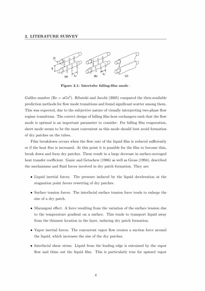
Figure 2.2: Schematic of liquid film breakdown for two different film flow rates
-
Figure 2.2 from Thome (2006) shows the observed liquid flow on a row of tubes for
two different film flow rates, including flow contraction and intertube flow modes. This
flow contraction was also observed and described by Fujita and Tsutsui (1998) . They
investigated breakdown of falling films with R-11 on plain tubes and defined a wetted
area fraction p as a function of the heat flux, flow rate and tube location.
5
2. LITERATURE SURVEY
2.3 Heat transfer mechanisms in falling films
According to Rohsenow et al. (1985), the heat transfer resistance in a falling film resides
in a thin thermal layer adjacent to the wall. This layer is approximately equal to the
residual film thickness. Furthermore, outside of the thermal boundary layer, the mixing
action of the interfacial waves ensures that a relatively constant film temperature is
obtained. When dealing with saturated falling films, convective heat transfer leads to
evaporation at the liquid-vapor interface. When the heat flux is increased, nucleate-
boiling begins. In the same study, it was reported that boiling occurs first on the lower
side of the tube, near the downstream stagnation point. Vapor bubbles grow in the film
and are carried along by the film flow. Thus, both thin-film evaporation and nucleate
boiling participate in the heat transfer process, depending on the heat flux and the
liquid flow rate.
Chyu and Bergles (1985) defined three heat transfer regions for falling film evap-
orative heat transfer. At the top of the tube is the jet impingement region, a small
region in which the heat transfer coefficient is relatively high due to liquid feed from
the top of the tube. In the thermally developing region, the film is superheated from
its uniform saturation temperature to a fully developed profile. Finally, in the fully
developed region, all of the additional heat transfer goes to evaporation at the liquid-
vapor interface, as long as no nucleate boiling occurs within the film. The convective
and boiling heat transfer regimes have to be considered separately because the two heat
transfer mechanisms are different.
In the heat exchanger we have natural convection due to local density gradients
within the heat exchanger. At low flow rates, these natural convection effects become
evident. Although the liquid refrigerant is drawn downwards by gravity, some of the va-
por in the heat exchanger moves upwards due to localized natural convection. However,
this heat transfer mechanism is very small and can be neglected.
2.4 Falling film enhancement
A great variety of enhancement techniques have been developed and applied to hori-
zontal falling film evaporators: structured surfaces (porous metallic surfaces, knurled
6
2.5 Single-array heat transfer studies
tubes), rough surfaces (ribbed or grooved tubes) and extended surfaces (circumferen-
tial or helical fins). All these attempts have been made to improve the heat transfer
performance.
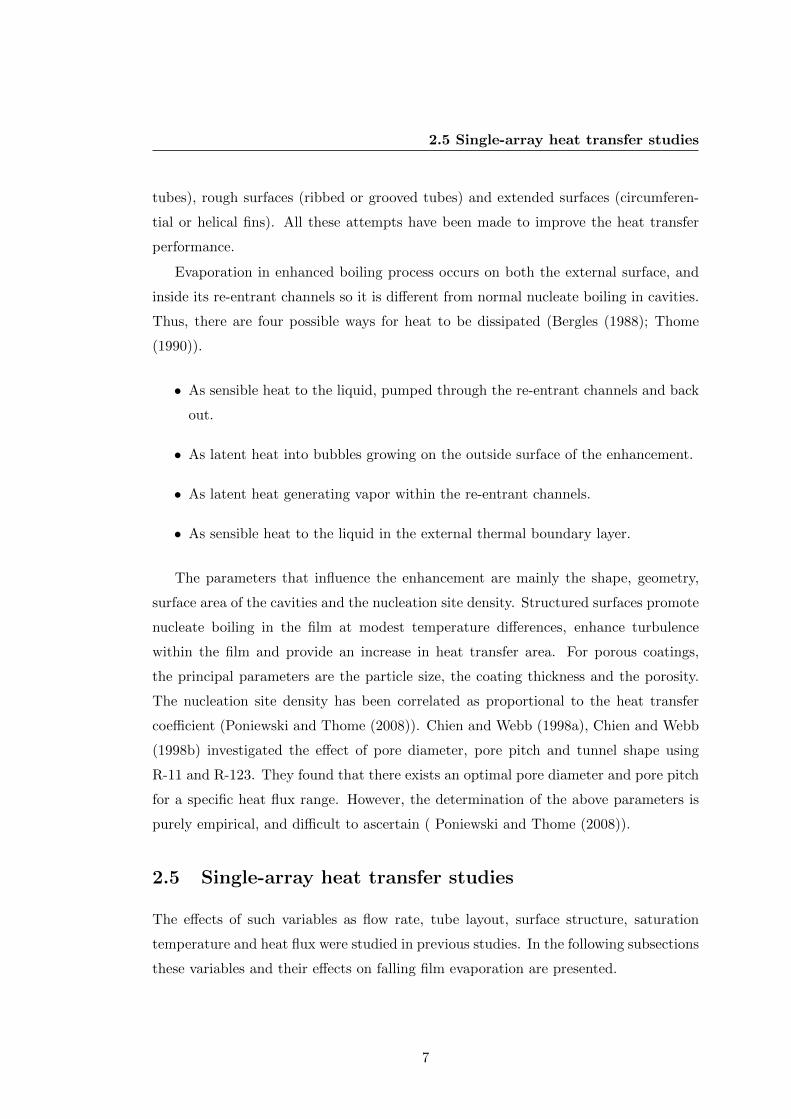
Evaporation in enhanced boiling process occurs on both the external surface, and
inside its re-entrant channels so it is different from normal nucleate boiling in cavities.
Thus, there are four possible ways for heat to be dissipated (Bergles (1988); Thome
(1990)).
• As sensible heat to the liquid, pumped through the re-entrant channels and back
out.
• As latent heat into bubbles growing on the outside surface of the enhancement.
• As latent heat generating vapor within the re-entrant channels.
• As sensible heat to the liquid in the external thermal boundary layer.
The parameters that influence the enhancement are mainly the shape, geometry,
surface area of the cavities and the nucleation site density. Structured surfaces promote
nucleate boiling in the film at modest temperature differences, enhance turbulence
within the film and provide an increase in heat transfer area. For porous coatings,
the principal parameters are the particle size, the coating thickness and the porosity.
The nucleation site density has been correlated as proportional to the heat transfer
coefficient (Poniewski and Thome (2008)). Chien and Webb (1998a), Chien and Webb
(1998b) investigated the effect of pore diameter, pore pitch and tunnel shape using
R-11 and R-123. They found that there exists an optimal pore diameter and pore pitch
for a specific heat flux range. However, the determination of the above parameters is
purely empirical, and difficult to ascertain ( Poniewski and Thome (2008)).
2.5 Single-array heat transfer studies
The effects of such variables as flow rate, tube layout, surface structure, saturation
temperature and heat flux were studied in previous studies. In the following subsections
these variables and their effects on falling film evaporation are presented.
7
2. LITERATURE SURVEY
2.5.1 Saturation temperature effect
Fletcher et al. (1974), Fletcher et al. (1975), Parken et al. (1990) and Armbruster and
Mitrovic (1995) observed, in the convective evaporation regime, an increase in per-
formance with increasing saturation temperature. This increase was related to the
variation in viscosity with temperature, and thus to the film thickness. In the boil-
ing regime, the effect of saturation temperature is not as clear. The results of Zeng
et al. (1996) indicated an increase in heat transfer coefficient, while Parken et al. (1990)
observed an opposite behavior under certain conditions. Ribatski and Jacobi (2005)
postulated that two competing effects can increase or decrease the heat transfer coeffi-
cient, namely, an increase of the activated nucleation site density with temperature, or
conversely, bubble growth inhibition due to a steeper temperature profile.
2.5.2 Layout effect
For non-boiling conditions, Parken and Fletcher (1982) measured a higher heat transfer
coefficient for smaller tube diameters. The respective proportion of the impingement
region on the overall flow area increases with decreasing diameter, resulting in better
performance. Such a noticeable diameter effect is not expected when nucleate boiling
is dominant.
2.5.3 Flow rate effect
An increase of heat transfer performance with increasing flow rate was observed by
Ganic and Roppo (1980) under strictly convective boiling evaporation conditions. How-
ever, under nucleate boiling conditions, the heat transfer coefficient was found to be
independent of the flow rate, as observed by Chyu and Bergles (1987), as well as by
Moeykens and Pate (1994), Moeykens et al. (1995a) and Moeykens et al. (1995b).
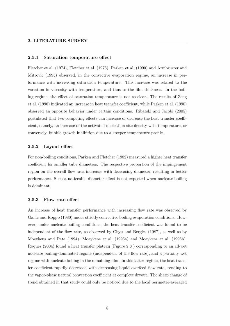
Roques (2004) found a heat transfer plateau (Figure 2.3 ) corresponding to an all-wet
nucleate boiling-dominated regime (independent of the flow rate), and a partially wet
regime with nucleate boiling in the remaining film. In this latter regime, the heat trans-
fer coefficient rapidly decreased with decreasing liquid overfeed flow rate, tending to
the vapor-phase natural convection coefficient at complete dryout. The sharp change of
trend obtained in that study could only be noticed due to the local perimeter-averaged
8
2.5 Single-array heat transfer studies
values of heat transfer coefficient that were measured. When tube-length averaged val-
ues were measured as in all the other studies, a monotonic increasing trend was always
found.
Figure 2.3: Schematic of the variation of heat transfer coefficient with flow rate
for falling film evaporation -
2.5.4 Heat flux effect
Based on the studies of Fujita and Tsutsui (1995) as well as that of Hu and Jacobi
(1996), the heat transfer performance for convective evaporation was not affected by
the heat flux. However, in nucleate boiling dominated conditions, higher heat transfer
coefficients were measured at higher heat fluxes due to increased nucleation site density
(Moeykens and Pate (1994), Zeng et al. (1996)). The measured variation of heat transfer
coefficient with heat flux was particularly high for low reduced-pressure fluids (Fletcher
et al. (1974)).
2.5.5 Enhanced surfaces
Surface modifications previously investigated include the use of porous structures and
structured surface geometries (micro and macro). Each of these techniques has been
9
2. LITERATURE SURVEY
shown to enhance heat transfer under certain conditions. The bubble growth mecha-
nism on an enhanced surface is different from that on plain surface, because the liquid
is mainly evaporated inside the tunnel for structured surfaces, while evaporation oc-
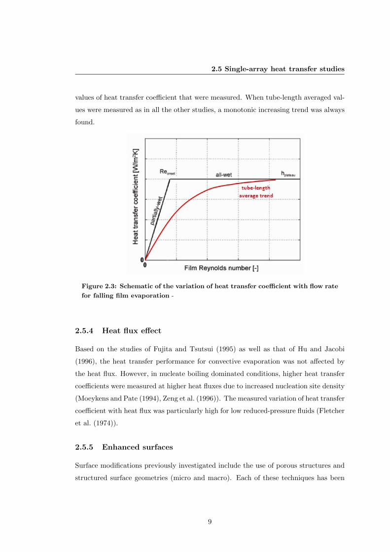
curs on the microlayer for the plain tube. Chien and Webb (1998a) tested enhanced
surfaces similar to the Turbo-B using R-11 and R-123. It was observed that, at low
heat flux, the tubes having smaller total open areas (that is, the sum of the cavity
areas) gave higher heat transfer coefficients. At higher heat fluxes, tubes having larger
total open areas yielded higher heat transfer performance. They reported a cross-over
characteristic between the two areas. If the total open area was too large at low heat
flux, the re-entrant tunnels became flooded by liquid and the heat transfer coefficient
decreased. If the total open area was too small at high heat fluxes, the tunnels dried
out due to inadequate liquid supply. Figure 2.4 represents this cross-over characteristic
as reported by Chien and Webb (1998a). Chien and Webb (1998b) also performed a
visualization study that supported these trends.
Figure 2.4: Cross-over characteristics of pored enhanced tubes -
Moeykens et al. (1995a) observed that enhanced boiling surfaces gave higher per-
formance than finned tubes but lower performance than enhanced condensing surfaces
used for evaporation. They noted an increase of heat transfer coefficient with heat flux
up to a specific heat flux, after which, with any further increase in heat flux, the heat
transfer coefficient decreased. This was probably due to partial dryout. Roques and
10
2.5 Single-array heat transfer studies
Thome (2007a) and Roques and Thome (2007b) tested three different enhanced sur-
faces: Gewa-B, Turbo- Bii and High-Flux. Similar trends for each surface were found,
as well as a strong dependence of the heat transfer on heat flux. The High-Flux tube
achieved up to three times better performance than the other tubes tested. A falling
film multiplier, Kff , was defined as the ratio between falling film evaporation and pool
boiling heat transfer coefficients on the same tube, and gave values between 1 and 2,
depending on the enhanced surface and the experimental conditions. In general, at low
heat fluxes, falling film achieves better performance than pool boiling. This might be
due to enhanced convective effects in the falling film. At high heat fluxes, nucleate
boiling was the dominant heat transfer mode; the convective effect tended to disappear
and the performances became comparable to those in pool boiling.
Habert (2009) tested three enhanced surfaces, the Gewa-B4, Turbo-EDE2 and the
Gewa-C LW, a condensation tube. The tests were performed using R-134a and R-236fa.
Tests in single-array mode, similar to those of Roques (2004) were performed. Using the
Gewa-C LW, Kff values of 2.53 were found near the onset-of-dryout Reynolds number
using R-134a and R-236fa respectively, at a heat flux of 20 kW/m2. However, most
of the data lie close to 1, indicating similar performance between falling film and pool
boiling. The performance of the tube did not vary much with choice of refrigerant. Both
the Gewa-B4 and the Turbo-EDE2 show similar trends to the previous generation’s
(that is, tubes tested by Roques (2004)), however, due to the improved performance,
the uncertainty in the measurements also increased. Heat transfer coefficients close
to those measured by Roques for the High-Flux tube were measured. The falling film
multiplier varied between 1 and 2, with falling film performing best at lower heat fluxes,
as shown in previous studies.
Christians (2010) tested two more surfaces, the Turbo-B5 and Gewa-B5, using re-
frigerants R-134a and R-236fa in both pool boiling and falling film evaporation. Chris-
tians observed that in pool boling, the tubes performed better than the tubes tested
by Roques (2004), and showed less dependance on the applied heat flux. In the terms
of refrigerant, it was seen that R-134a outperformed R-236fa, as was expected, since
these tubes are designed for use with R-134a.
11
2. LITERATURE SURVEY
2.6 Falling film heat transfer prediction methods
Previous heat transfer studies on falling film evaporation have yielded various semi-
empirical and empirical prediction methods. These methods have taken into account
both convective and nucleate boiling components. In the literature, analytical predic-
tions are mainly made for non nucleate boiling heat transfer only. More information
about previous heat transfer studies can be found in the studies developed by: Lorenz
and Yung (1979), Chyu and Bergles (1987), Fujita and Tsutsui (1995) and Chien and
Cheng (2006).
More recently, the study of Ribatski and Thome (2007) developed a predictive
method for plain tubes using R-134a to characterize both local dryout and non dryout
conditions. They defined an objective criterion to characterize the onset of dryout
based on Kff . The onset of dryout (i.e. initial formation of dry patches) was defined
by a drastic decrease of the heat transfer coefficient with decreasing film flow rate and
a decrease in the average heat flux. This selection criterion was used to segregate
the data as either being under partial dryout or non dryout conditions. In this new
method for partial dryout, the heat transfer area was divided into wet and dry regions
respectively governed by nucleate boiling and vapor natural convection heat transfer.
The local external heat transfer coefficient and heat flux were defined by:
ho = hwetF + hdry(1− F ) (2.1)
qo = qwetF + qdry(1− F ) (2.2)
where F represents the apparent wet area fraction defined as the ratio between the
wet area and the total area. Based on a regression analysis of the non dryout data, a
simple correlation of hwet was obtained. The values of hdry were calculated using the
Churchill and Chu (1975) correlation for free convection described in Gnielinski (1975),
assuming quiescent vapor conditions within the falling film evaporator.
By combining the above mentioned parameters values of F were backed out and
correlated as a function of the flow rate:
F = aRebtop (2.3)
12
2.6 Falling film heat transfer prediction methods
The method works reasonably well, with 76% of data predicted within ± 30% for
dryout conditions and 96% predicted within ± 30% for non dryout conditions. The
prediction method captures well the heat flux effect on the heat transfer coefficient and
the onset of dryout.
Habert (2009) expanded the work begun by Ribatski and Thome (2007) and Roques
and Thome (2007a) by reformulating the form of the prediction of the Reynolds number
for onset of film dryout, and expanding the database to include R-134a, R-236fa and the
three enhanced tubes tested. The method proposed utilizes fewer empirical constants.
The form of the method is
Reonset = a
(qoD
µlhlv
)b
(2.4)
The experimental data points measured by Roques and Thome (2007a), as well as
new data were utilized to obtain new simplified correlations for the onset of dryout
for all tubes and refrigerant combinations tested to date. The method of Ribatski and
Thome (2007) was simplified from
ho = hwetF + hdry(1− F ) (2.5)
to just
ho = hwetF (2.6)
because the heat transfer coefficient for the dry region, obtained using the natural
convection correlation of Churchill and Chu (1975), contributes little to the combined
heat transfer coefficient ho. The calculation of the apparent wet fraction F was also
simplified to get:
F =RetopReonset
for (Re < Reonset) (2.7)
F = 1 for (Re > Reonset) (2.8)
Finally, he correlated the falling film multiplier Kff as:
Kff = c
(qoqcrit
)d
(2.9)
13
2. LITERATURE SURVEY
From the definition of the falling film multiplier, the falling film heat transfer coef-
ficient is known if the pool boiling correlation is known. And, using the apparent wet
fraction, the partially wet heat transfer coefficient can be calculated. This method,
applied to the data measured during his experimental campaign, yielded an average of
85% of his data predicted to within ± 20%, including all four tubes tested and both
refrigerants utilized.
Christians (2010) utilized the results obtained in pool boiling, single-array and
bundle falling film evaporation during his study and the results of the previous studies
of Roques and Thome (2007a) and Habert (2009) to generate prediction methods for
heat transfer performance. These include a prediction method for single-tube pool
boiling, another for the onset of dryout and two methods for falling film evaporation
heat transfer. These prediction methods are the ones that were utilized in this study.
They are presented in the following sections.
2.6.1 Christians (2010) pool boiling prediction method
Before this method there were fourteen different correlations for the fourteen different
saturation pressure-specific tests performed at LTCM. A dimensional analysis of a
typical pool boiling experiment results in nine variables, of which three are independent.
These are the diameter Do, the gravitational acceleration force g, the density difference
ρl − ρv, the thermal conductivity kl, the latent heat hlv, the heat flux qo and the
saturation pressure psat or Tsat. Thus, it is expected that six different π groups exist.
By taking Do, g and ρl − ρv as the building blocks of the π groups, we find
π0 =g(ρl − ρvD2
0)
σ(2.10)
π1 =gD3
0(ρl − ρv)2
µ2l(2.11)
π2 =hlvdD0
(2.12)
π3 =psat
gD0(ρl − ρv)(2.13)
14
2.6 Falling film heat transfer prediction methods
π4 = (gD0)32ρl − ρvq0
(2.14)
π5 =
(g3
Do
)12 klTsat
(ρl − ρv)13
(2.15)
The non-dimensional groups π2, π3 and π4 can be arranged together to give a new
π group
π6 =q2o
hlvp2sat
(2.16)
where π6 gives an effective rate of bubble generation (which indicates the amount
of liquid pumping intake that occurs into the 3D enhancement) and the heat flux
dependence on the saturation pressure (also a type of flow rate).
To further generalize this form, and to thus predict the heat transfer performance
of several tube/refrigerant combinations, a tube-specific factor was included as well as
the Nusselt number to give the prediction method the correct units of Wm−2K−1. This
results in
hpb = aoπa16 G
a2t−s
(klDo
)(2.17)
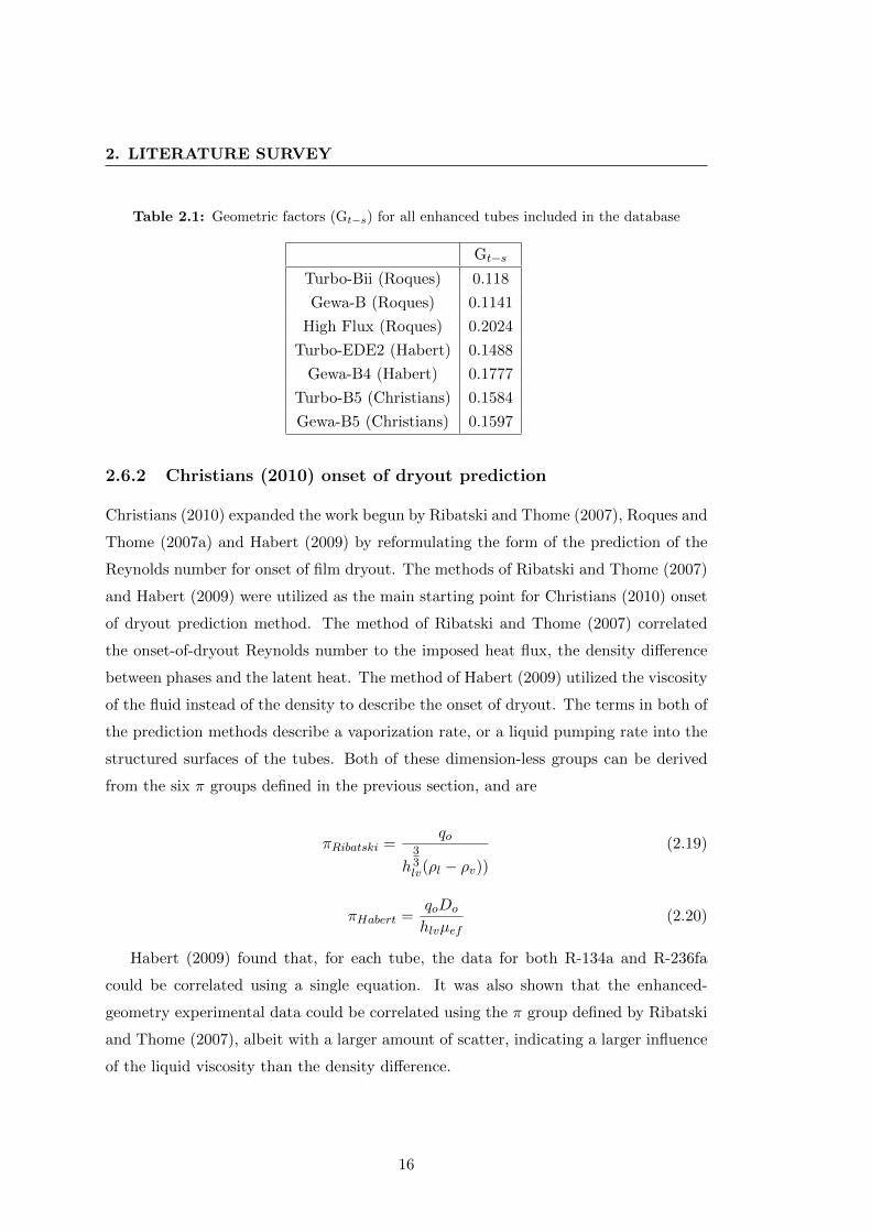
The equation above has three unknowns and one tube-specific variable Gt−s to
predict the heat transfer coefficient of seven different tubes (six of them 3D-enhanced
tubes and the High Flux tube) using two different refrigerants (R-134a and R-236fa).
The unknowns were fit using a non-linear least squares minimization program. The
tube-specific factor Gt−s was also a variable in the minimization scheme. The achieved
factor is indicative of the actual surface enhancement and its effect on the heat transfer.
The tube-specific factors obtained by Christians (2010) for each tube type are presented
in Table 2.1 .
The parameters from the converged minimization result in the following equation:
hpb = 99976π−0.1286 G1.658
t−s
(klDo
)(2.18)
This single correlation predicts 96% of the data within ±20%.
15
2. LITERATURE SURVEY
Table 2.1: Geometric factors (Gt−s) for all enhanced tubes included in the database
Gt−s
Turbo-Bii (Roques) 0.118
Gewa-B (Roques) 0.1141
High Flux (Roques) 0.2024
Turbo-EDE2 (Habert) 0.1488
Gewa-B4 (Habert) 0.1777
Turbo-B5 (Christians) 0.1584
Gewa-B5 (Christians) 0.1597
2.6.2 Christians (2010) onset of dryout prediction
Christians (2010) expanded the work begun by Ribatski and Thome (2007), Roques and
Thome (2007a) and Habert (2009) by reformulating the form of the prediction of the
Reynolds number for onset of film dryout. The methods of Ribatski and Thome (2007)
and Habert (2009) were utilized as the main starting point for Christians (2010) onset
of dryout prediction method. The method of Ribatski and Thome (2007) correlated
the onset-of-dryout Reynolds number to the imposed heat flux, the density difference
between phases and the latent heat. The method of Habert (2009) utilized the viscosity
of the fluid instead of the density to describe the onset of dryout. The terms in both of
the prediction methods describe a vaporization rate, or a liquid pumping rate into the
structured surfaces of the tubes. Both of these dimension-less groups can be derived
from the six π groups defined in the previous section, and are
πRibatski =qo
h33lv(ρl − ρv))
(2.19)
πHabert =qoDo
hlvµef(2.20)
Habert (2009) found that, for each tube, the data for both R-134a and R-236fa
could be correlated using a single equation. It was also shown that the enhanced-
geometry experimental data could be correlated using the π group defined by Ribatski
and Thome (2007), albeit with a larger amount of scatter, indicating a larger influence
of the liquid viscosity than the density difference.
16
2.6 Falling film heat transfer prediction methods
Christians (2010) generalized the form proposed by Habert (2009) by multiplying
it with the geometric factor Gt−s with the goal of minimizing the number of empirical
constants required to predict the performance of the tubes. Thus, the goal was to
obtain a single method in which, by changing only Gt−s, the onset of dryout can be
predicted. The form of the equation to be minimized is
Reonset,corr = a0
(qoDo
hlvµref
)a1
Ga2t−s (2.21)
From the experimental database a Gt−s was applied to each tube and the correlation
constant (a0, a1, a2) were found by applying a non-linear minimization scheme.
Reonset,corr = 20.721
(qoDo
hlvµref
)1.04
G1.04t−s (2.22)
This single correlation predicted 95% of the database within 20%. The correlation
is almost linearly proportional to the non-dimensional group, and is a weak function of
the tube-specific factor, as confirmed by the experimental results (Christians (2010))
that showed that the data are not dissimilar. The method underpredicts roughly as
much data as it overpredicts.
Once a specific tube has been chosen (i.e. the correct Gt−s is selected), the only
test-specific variable becomes the heat flux, as the rest are thermo-physical properties
set by the saturation temperature or the nominal outer diameter of the tube. The
fact that the onset-of-dryout Reynolds number varies almost linearly with the heat flux
shows that the experimental data trends were adequately captured by this formulation.
Moreover, utilizing the same Gt−s tube-specific factors obtained for pool boiling allows
us to minimize the number of variables needed to satisfactorily predict the experimental
data.
2.6.3 Plateau heat transfer coefficient prediction method
Roques and Thome (2007a) developed a method in which the plateau heat transfer
could be calculated using the pool boiling curves and the falling film multiplier as a
function of the tube pitch, as well as the test and critical heat fluxes, leading to an
equation that had six unknowns for each tube/refrigerant combination. The method of
Ribatski and Thome (2007) utilized a single nucleate boiling-type equation to predict
17
2. LITERATURE SURVEY
the heat transfer of smooth tubes only. Finally, Habert (2009) correlated the experi-
mental data as a power function of the plateau heat flux (qwet in his nomenclature),
leading to two unknowns per tube/refrigerant combination. Utilizing the same three
groups as in the pool boiling analysis (the nominal diameter Do, g and the difference
in density between phases (ρl-ρv)) results in
π7 =Γ2
gD3o (ρl − ρv)2
(2.23)
Non-dimensional groups π3 and π7 ( (2.13) and (2.23) ) can be combined to formu-
late the refrigerant film Reynolds number. This additional group is nevertheless useless
as a predictor for the plateau heat transfer coefficient, as the very name ‘plateau coef-
ficient’ implies that there is no trend to be found with respect to the refrigerant film
Reynolds number. However, the combination of π groups π1, π2 and π4 result in
π8 =q2oDo
h52lvµref (ρl − ρv)
(2.24)
Equation (2.24) suggests that the results of both refrigerants should be able to be
predicted by a single method. As was done with the onset-of-dryout prediction, the
method was generalized by multiplying by the tube-specific factor found in the pool
boiling correlation, and by klD−1o to give the correlation a Nusselt number. Finally,
using a non-linear minimization scheme on the filtered experimental data results in
hplateauDo
kl= 9.623 · 104
q2oDo
h52lvµref (ρl − ρv)
0.0328
G1.2449t−s (2.25)
The above equation predicts 91% of the plateau heat transfer coefficient data within
±20%. Again, the only unknown that changes is the tube-specific Gt−s found in Table
2.1
This above new equation is of interest if the user requires a direct calculation of
the falling film heat transfer coefficient in a thermal design. Otherwise, a falling film
multiplier can be combined with the pool boiling correlation to generate a second
alternative method.
Thus, a prediction method for the Falling film multiplier Kff is proposed later
(in the following section). Using the above method would be more accurate due to a
18
2.6 Falling film heat transfer prediction methods
smaller propagation of error. However, since pool boiling testing is relatively easy to
do compared to falling film tests, if a tube’s performance can be characterized in pool
boiling, the falling film multiplier method can be used to easily predict the plateau heat
transfer coefficient.
2.6.4 Christians (2010) falling film evaporation heat transfer predic-
tions
The experimental fully wet heat transfer coefficients were utilized by Christians (2010)
to generate a single method to calculate the plateau heat transfer coefficient. With
respect to the partially dry heat transfer coefficient data, the method developed by
Habert (2009) to calculate the apparent wet fraction area is utilized. Habert (2009)
simplified the method of Ribatski and Thome (2007) and showed comparable results
to both those their results and those of Roques (2004). The method is
F =RetopReonset
for (Re < Reonset) (2.26)
F = 1 for (Re > Reonset) (2.27)
The onset-of-dryout Reynolds number to be utilized in this method corresponds
to the new predictive correlation of Equation (2.22), and the experimental Reynolds
number used is the Reynolds number calculated at the top dead center of each tube.
The predicted heat transfer coefficients are calculated using
hff,pred = Fhplateau (2.28)
The predictive methods presented in the following sections utilize single-array and
bundle data, and are valid for both conditions.
2.6.5 Falling film multiplier
The form proposed by Christians (2010) to correlate the falling film multiplier is similar
to the methods proposed previously, in that the tube-specific Gt−s factors from Table
2.1 are utilized to serve as the differentiator (between tubes) in an otherwise constant
equation (i.e. only one empirical constant, Gt−s ). The ratio of local heat flux to the
19
2. LITERATURE SURVEY
critical heat flux defined by Kutateladze (1948) is also utilized. Using a non-linear
minimization scheme, we find that
Kff = 65.3
((gD)
32 )ρl − ρvqo
)0.4585( qoqcrit
)0.6204
G−0.024t−s (2.29)
The above prediction method can be utilized to predict 88% of the experimental
data within an error band of 20%.
2.7 Conclusions
Falling film evaporation on horizontal tubes is a complex process. Several parameters
affect the heat transfer characteristics of this process, including the choice of refrigerant,
the type of tube utilized, the mass flux and the fluid properties (at the temperature and
pressure utilized) among others. Although the main parameters have been identified,
a general and mechanistic model of falling film heat transfer has yet to be developed.
Experimental correlations as the ones presented in this chapter only select some of the
parameters and factors that affect the heat transfer. Furthermore, the available tube
geometries studied in detail are limited, both in numbers and in type of geometry used.
Another major difficulty found in the generation of experimental correlations has been
the differentiation between purely fluid-related effects and those that arise from the
structure (tube) utilized.
20
3
Experimental setup
3.1 Introduction
All the tests were done in the existing LTCM falling film and pool boiling facilities. In
this chapter the design, operation and instrumentation of both facilities are discussed.
The falling film experiments have been made on the original test facility developed
and modified by Roques (2004), Gstohl (2004), Habert (2009) and Christians (2010) .
The pool boiling facility was developed and modified by Casciaro and Thome (2001),
Thome and Robinson (2006), Agostini (2008) and van Rooyen (2011)
3.2 Falling film facility
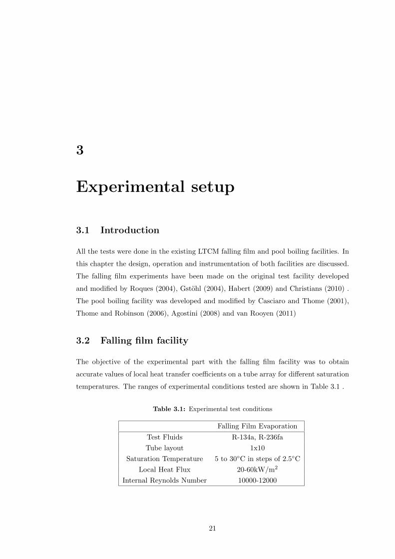
The objective of the experimental part with the falling film facility was to obtain
accurate values of local heat transfer coefficients on a tube array for different saturation
temperatures. The ranges of experimental conditions tested are shown in Table 3.1 .
Table 3.1: Experimental test conditions
Falling Film Evaporation
Test Fluids R-134a, R-236fa
Tube layout 1x10
Saturation Temperature 5 to 30◦C in steps of 2.5◦C
Local Heat Flux 20-60kW/m2
Internal Reynolds Number 10000-12000
21
3. EXPERIMENTAL SETUP
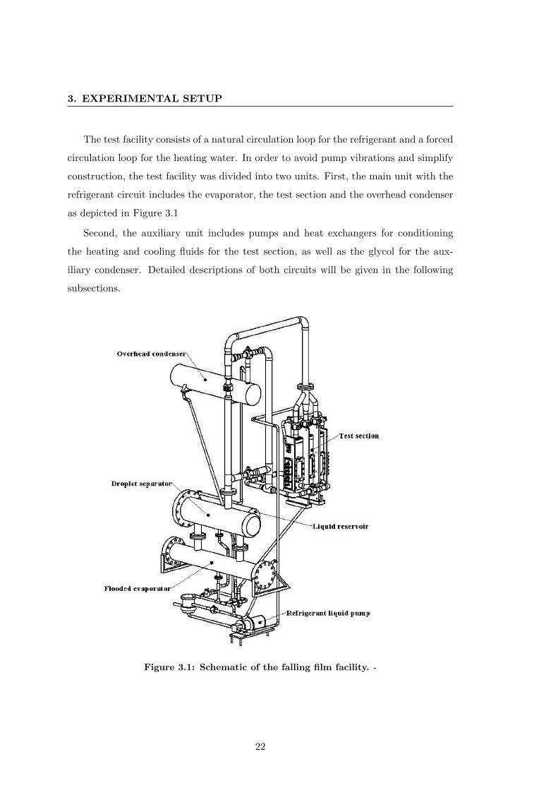
The test facility consists of a natural circulation loop for the refrigerant and a forced
circulation loop for the heating water. In order to avoid pump vibrations and simplify
construction, the test facility was divided into two units. First, the main unit with the
refrigerant circuit includes the evaporator, the test section and the overhead condenser
as depicted in Figure 3.1
Second, the auxiliary unit includes pumps and heat exchangers for conditioning
the heating and cooling fluids for the test section, as well as the glycol for the aux-
iliary condenser. Detailed descriptions of both circuits will be given in the following
subsections.
Figure 3.1: Schematic of the falling film facility. -
22
3.2 Falling film facility
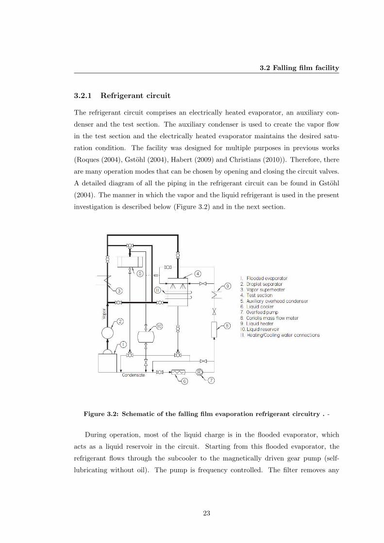
3.2.1 Refrigerant circuit
The refrigerant circuit comprises an electrically heated evaporator, an auxiliary con-
denser and the test section. The auxiliary condenser is used to create the vapor flow
in the test section and the electrically heated evaporator maintains the desired satu-
ration condition. The facility was designed for multiple purposes in previous works
(Roques (2004), Gstohl (2004), Habert (2009) and Christians (2010)). Therefore, there
are many operation modes that can be chosen by opening and closing the circuit valves.
A detailed diagram of all the piping in the refrigerant circuit can be found in Gstohl
(2004). The manner in which the vapor and the liquid refrigerant is used in the present
investigation is described below (Figure 3.2) and in the next section.
Figure 3.2: Schematic of the falling film evaporation refrigerant circuitry . -
During operation, most of the liquid charge is in the flooded evaporator, which
acts as a liquid reservoir in the circuit. Starting from this flooded evaporator, the
refrigerant flows through the subcooler to the magnetically driven gear pump (self-
lubricating without oil). The pump is frequency controlled. The filter removes any
23
3. EXPERIMENTAL SETUP
particles from the liquid refrigerant and also contains a refrigerant drying cartridge.
The subcooler is used at the pump entrance to avoid cavitation. Bypass piping is also
used together with the frequency controller to achieve the desired liquid flow rate. For
very low flow rates, in order to avoid oscillations, the bypass is opened rather than using
very flow frequencies with the gear pump. After the pump, the liquid goes through a
vibration absorber, a Coriolis mass flow meter, and an electric heater. The heater is
used to take the liquid close to the saturation conditions at the test section’s inlet. At
this point, the liquid enters the test section and is distributed uniformly on the heated
tubes. Special care has been taken to achieve uniform distribution and more detail is
provided in section 3.2.3.1 Once the liquid leaves the distributor, it falls on top of the
heated tubes where it is partially evaporated and the residual liquid leaving the test
section flows via gravity back to the flooded evaporator. The vapor refrigerant circuit
is a natural circulation loop. The vapor is evaporated in the lower part of the circuit
and condensate is formed in the upper parts. The liquid flows back from the auxiliary
condenser to the flooded evaporator by gravity. The test facility offers three different
possibilities for the vapor flow: downwards, upwards, and quiescent vapor flow. This
last mode was chosen for use in this study because in this mode, the vapor leaves the
test section very slowly (less than 1 m/s)( Christians (2010)), minimizing any vapor
shear effects.
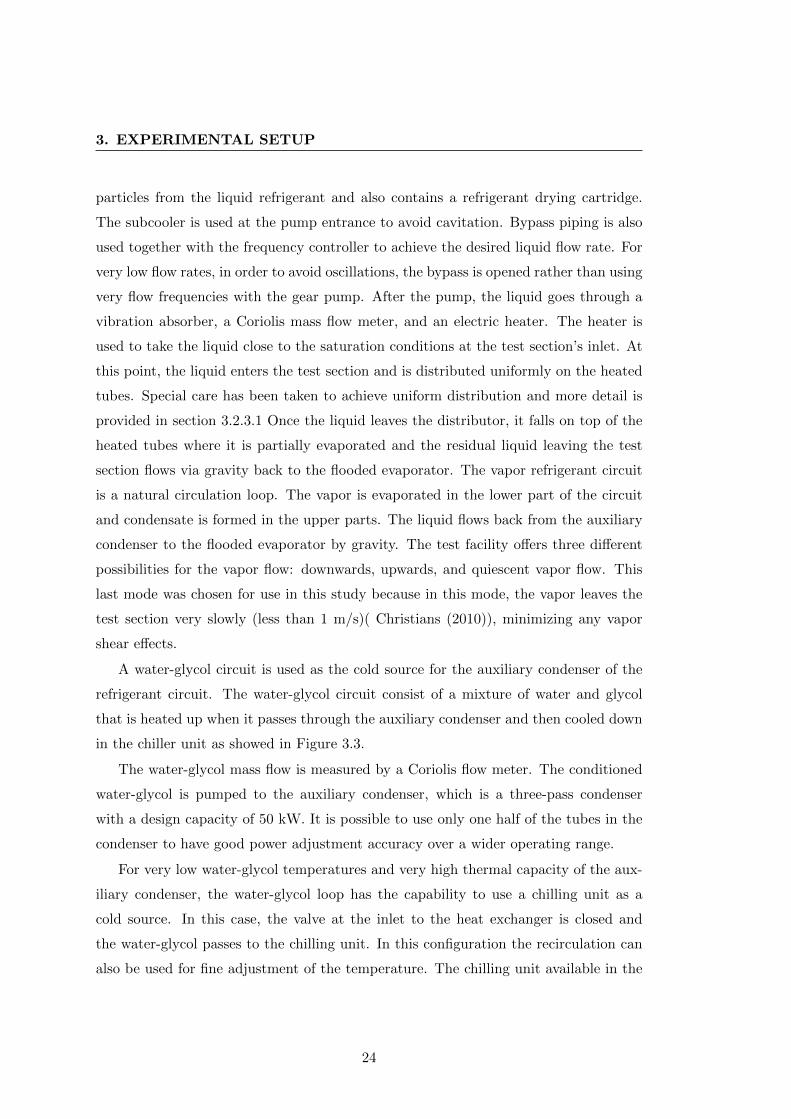
A water-glycol circuit is used as the cold source for the auxiliary condenser of the
refrigerant circuit. The water-glycol circuit consist of a mixture of water and glycol
that is heated up when it passes through the auxiliary condenser and then cooled down
in the chiller unit as showed in Figure 3.3.
The water-glycol mass flow is measured by a Coriolis flow meter. The conditioned
water-glycol is pumped to the auxiliary condenser, which is a three-pass condenser
with a design capacity of 50 kW. It is possible to use only one half of the tubes in the
condenser to have good power adjustment accuracy over a wider operating range.
For very low water-glycol temperatures and very high thermal capacity of the aux-
iliary condenser, the water-glycol loop has the capability to use a chilling unit as a
cold source. In this case, the valve at the inlet to the heat exchanger is closed and
the water-glycol passes to the chilling unit. In this configuration the recirculation can
also be used for fine adjustment of the temperature. The chilling unit available in the
24
3.2 Falling film facility
Figure 3.3: Schematic of the forced-circulation water-glycol circuit -
laboratory can provide glycol at -20◦C and has a maximum continuous cooling capacity
of 80 kW.
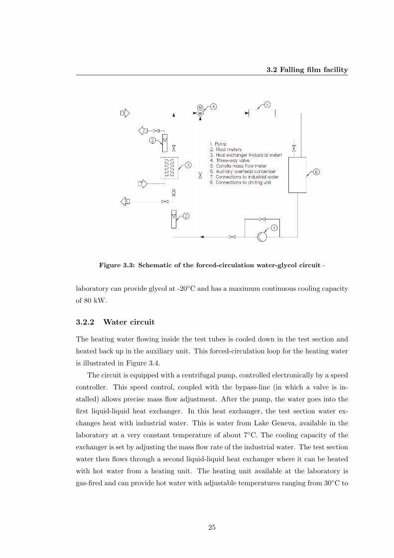
3.2.2 Water circuit
The heating water flowing inside the test tubes is cooled down in the test section and
heated back up in the auxiliary unit. This forced-circulation loop for the heating water
is illustrated in Figure 3.4.
The circuit is equipped with a centrifugal pump, controlled electronically by a speed
controller. This speed control, coupled with the bypass-line (in which a valve is in-
stalled) allows precise mass flow adjustment. After the pump, the water goes into the
first liquid-liquid heat exchanger. In this heat exchanger, the test section water ex-
changes heat with industrial water. This is water from Lake Geneva, available in the
laboratory at a very constant temperature of about 7◦C. The cooling capacity of the
exchanger is set by adjusting the mass flow rate of the industrial water. The test section
water then flows through a second liquid-liquid heat exchanger where it can be heated
with hot water from a heating unit. The heating unit available at the laboratory is
gas-fired and can provide hot water with adjustable temperatures ranging from 30◦C to
25
3. EXPERIMENTAL SETUP
Figure 3.4: Schematic of the forced-circulation loop for the heating water -
90◦C with a maximum capacity of 160 kW. The heat exchanged in this heat exchanger
is controlled by the flow rate of the hot water. An electronically actuated, computer-
controlled valve sets this flow rate based on the test section water temperature at the
outlet of the heat exchanger. The water temperature at the test section inlet is thus
automatically maintained constant when the flow rate is changed or if there are any
temperature variations in the water provided by the heating unit. At this point, the
water for the test section is well conditioned in terms of stability of its temperature
and flow rate. The total mass flow rate is finally measured with a Coriolis mass flow
meter. The main water line is then split into the sub-circuits of the test section. Each
sub-circuit has its own float flow meter and valve to control its flow rate and thus set the
water distribution uniformly between the sub-circuits. The goal is to achieve the same
flow rate in all sub-circuits. There are five sub-circuits and each one can be included
(or excluded) in the main circuit with two three-way valves each. A sub-circuit usually
has two tube passes, i.e. water goes in a copper tube in one direction and comes back
through the copper tube just above in the opposite direction within the test section.
26
3.2 Falling film facility
With this setup, the water temperature profiles in the two tubes are opposed. The
quantity of liquid refrigerant evaporated after each two tubes in the test array is thus
nearly uniform along the tube length. Tests in other published projects often use only
one water pass, which creates a significant heat flux variation along the tubes, which
in turn creates an imbalance in the axial liquid film distribution and hence make those
data dependent on the test setup, which is to be avoided. After the test section, the
sub-circuits merge and the water flows back to the pump.
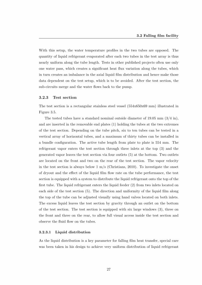
3.2.3 Test section
The test section is a rectangular stainless steel vessel (554x650x69 mm) illustrated in
Figure 3.5.
The tested tubes have a standard nominal outside diameter of 19.05 mm (3/4 in),
and are inserted in the removable end plates (1) holding the tubes at the two extremes
of the test section. Depending on the tube pitch, six to ten tubes can be tested in a
vertical array of horizontal tubes, and a maximum of thirty tubes can be installed in
a bundle configuration. The active tube length from plate to plate is 554 mm. The
refrigerant vapor enters the test section through three inlets at the top (3) and the
generated vapor leaves the test section via four outlets (5) at the bottom. Two outlets
are located on the front and two on the rear of the test section. The vapor velocity
in the test section is always below 1 m/s (Christians, 2010). To investigate the onset
of dryout and the effect of the liquid film flow rate on the tube performance, the test
section is equipped with a system to distribute the liquid refrigerant onto the top of the
first tube. The liquid refrigerant enters the liquid feeder (2) from two inlets located on
each side of the test section (5). The direction and uniformity of the liquid film along
the top of the tube can be adjusted visually using hand valves located on both inlets.
The excess liquid leaves the test section by gravity through an outlet on the bottom
of the test section. The test section is equipped with six large windows (3), three on
the front and three on the rear, to allow full visual access inside the test section and
observe the fluid flow on the tubes.
3.2.3.1 Liquid distribution
As the liquid distribution is a key parameter for falling film heat transfer, special care
was been taken in his design to achieve very uniform distribution of liquid refrigerant
27
3. EXPERIMENTAL SETUP
Figure 3.5: Schematic of the test section -
28
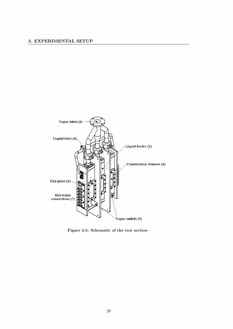
3.2 Falling film facility
along the tubes. The distributor is a rectangular box (554 x 200 x 20 mm)positioned
in the test section above the tubes. A cross sectional schematic of the liquid feeder is
given in Figure 3.6.
Figure 3.6: Schematic of the liquid distributor -
This liquid feeder has two main purposes:
• To distribute the nearly saturated liquid refrigerant uniformly along the top tube.
• To mimic the flow of an upper tube onto the top tube.
The liquid refrigerant enters on both sides at the top and is pre-distributed with a
13 mm internal diameter stainless steel pipe, in which there are holes oriented upwards
(1). The holes are 3 mm in diameter and spaced 5 mm center to center. Then, the
liquid flows through two layers of foam material compatible with R-134a and R-236fa.
The first is a 150 mm-tall layer of soft foam material (2). This is a polyurethane foam
with a pore diameter of 200 µm and 60 pores per inch. The second is a 10 mm-tall
layer of a filter plate (3), which is a polyethylene foam material with a pore diameter of
35 µm and a porosity of 37 %. This second layer is more compact and creates a larger
pressure drop to force good lateral distribution of the liquid. After this porous section,
the liquid reaches the bottom of the distributor, which is a removable machined brass
piece with 268 holes along its centerline (4). The diameter of these holes is 1.5 mm
and the center-to-center distance is 2 mm. The liquid distributor width is 550 mm. At
29
3. EXPERIMENTAL SETUP
high liquid flow rates, a continuous sheet leaves the distributor, but at low flow rates
the distribution of the droplets is not uniform. For this reason a half-tube was added
just below the distributor (5). It was machined from a plain stainless steel tube 20 mm
in diameter. The bottom of the half tube was machined to form a sharp edge. The
liquid falls locally along the half-tube and over flows on both sides. The sharp edge
forces the liquid to leave at the bottom of the half tube. By rotating the half tube, the
direction of the liquid leaving the tube at the edge can be adjusted to ensure that the
liquid falls exactly on the center of the top of the first test tube (6). The temperature
of the overfeed liquid is controlled by a heater to maintain its subcooling to less than
0.8 K.
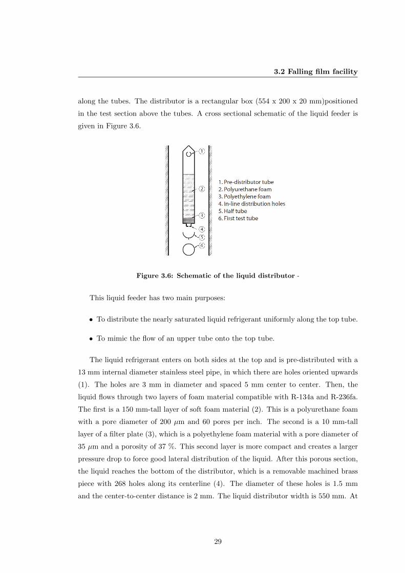
3.2.3.2 Tube layout
The facility permits different tube arrangements. In this study we used a single column
of ten tube (1x10) as shown in Figure 3.7.
Figure 3.7: Schematic of the tube layout. -
The dimensions and layout used for this study correspond to those recommended
by the industrial sponsors of the project. The tube pitch center-to-center was 22.3 mm,
allowing ten tubes to be installed. With a nominal tube diameter of 19.05 mm and inter-
tube spacings of 3.25 mm. Christians (2010) found that the results using a bundle of
30
3.2 Falling film facility
tubes and those using the single-array were the same, indicting that ’no-bundle effect’,
positive or otherwise, was present.
3.2.4 Measurements procedure
The 10-pass circuit is heated using the heating circuit; the heat flux on both sides was
controlled by the flow rate and the inlet temperature of the water. Previous studies
found a non-negligible difference ( equal to ± 0.5 K ) in the temperature between
the top and the bottom of the test section due to the additional pressure drop with
three active rows ( Christians (2010) ). The estimation of the saturation temperature
is thus adapted accordingly: a linear interpolation is made between the temperatures
obtained at the top and bottom to obtain the local saturation temperature at each
tube elevation. This assumption is commonly used in bundle heat exchangers analysis.
3.2.4.1 Data acquisition and control
All measurements were made using a computer attached to a data acquisition system
from National Instrument. The acquisition card is a PCI-MIO-16XE-50 with 16-bit
resolution and a maximum acquisition frequency of 10 kHz on a single channel. A
SCXI-1000 module with four bays is connected to this card. Each of the four bays is
equipped with a 32-channel voltage measurement card (SCXI-1102 card). The total
number of acquisition channels is thus 128. Each channel has a computer programmable
gain: one for 0 to 10 V signals (pressure transducers and mass flow meters), and 100
for low voltage signals (thermocouples). The signals can be adjusted to the 0 to 10
V range of the acquisition card. A 2 Hz low-pass frequency filter is also included to
reduce the measurement noise without affecting the steady-state measurements. At
the end of the acquisition chain, a terminal block is connected to the SCXI-1102 card.
Each card has its own terminal block. The cold junction for every thermocouple is
made in the terminal block at the socket. The material for this socket is copper for
both poles (+ and -). The continuity of the two different specific materials of the
thermocouple is broken at this point inside the terminal block. The temperature of
the 32 cold junctions is maintained uniform with a metallic plate and is measured via
a thermistor installed in the middle. Additionally, all the terminal blocks are isolated
in an electrical cupboard to avoid any external thermal influence. During a test, 100
acquisitions were made at a frequency of 50 Hz to measure a test parameter in a channel
31
3. EXPERIMENTAL SETUP
and the average of these 100 values was calculated during the acquisition. The result
is the measured value of the channel. In this way, any noise from alternating current
on the measured signal is removed. This value is stored and the system goes to the
next channel. With this measurement method, the theoretical channel measurement
frequency is 50 channels/s, but due to the switching time between channels, the actual
frequency is 30 channels/s. In total it takes 4.3 s to measure all the channels of the
acquisition system once. To obtain one experimental point, 30 such acquisition cycles
are recorded and averaged. Steady-state conditions were achieved after a minimum
settling time of 20 minutes between changing points and when the standard deviation
of the experimental conditions’ average values of heat flux, mass flow and saturation
temperature varied less than 0.1%. A second computer is used to control the test
facility with an identical SCXI system as used in the data acquisition computer. The
four bays of the SCXI-1000 module contain two cards for voltage measurement (SCXI-
1102 cards), one card for current measurement (SCXI-1102 card) and one card with six
output channels (SCXI-1124 card). These outputs are used to control the three-way
valves for the water-glycol, the hot water, the two electric heaters in the evaporator,
the liquid heater and the vapor superheater. Two PID controllers are programmed on
this computer: one for the electrical heating of the evaporator to control and stabilize
the saturation pressure in the test facility, and one for the hot water valve to control
and adjust the hot water temperature flowing through the test section. All parameters
are displayed online on the computer screens, and experimental parameters are also
calculated and displayed. These parameters include the water temperature profile,
local heat fluxes, heat transfer coefficients and PID status among others.
3.2.4.2 Measurements and accuracy
The objective of the experimental part of this work was to measure local external
heat transfer coefficients over a range of liquid film flow rates and heat fluxes. Local
heat transfer coefficients were obtained using the Christians (2010) modified Wilson
plot method. Meanwhile, to completely establish the experimental conditions, some
other parameters need to be measured directly or calculated from measured values.
The test section was instrumented in order to estimate the degree of subcooling and
check the homogeneity of the saturation conditions from top to bottom. The vapor
pressure in the test section is measured with two absolute pressure transducers. One
32
3.2 Falling film facility
is connected to the test section above the array of tubes and one below. The vapor
temperature above the tubes is measured with six thermocouples. Three are situated on
the front and three on the rear of the test section. They are 1 mm in diameter and the
junction is located in the middle between the test section wall and the distributor. The
temperature of the liquid entering the test section is measured with one thermocouple
inserted in each inlet. Below the array of tubes, three thermocouples 2 mm in diameter
are installed on the front of the test section. The junctions of these thermocouples are
situated in the middle between the front and rear side. The temperature of the vapor
leaving the test section is measured with one thermocouple in the vapor pipe on the
front after the two vapor outlets on the front joined and one at the same position on
the rear. The temperature of the liquid leaving the test section is measured with a
thermocouple inserted in the liquid outlet. The wall temperature of the test section is
measured with one thermocouple attached on the outside. All the physical properties
for water and refrigerants, R-134 and R-236fa, were estimated using REFPROP 8:0
(National Institute of Standards and Technology (2002)). The fluid database was
directly linked with MatLab, and the desired physical properties could be called in
realtime by the nested scripts inside of the LabView programs. Then knowing the
saturation pressure Psat, the saturation temperature was obtained based on the vapor
pressure curve. Two absolute pressure transducers (0 - 10 bars) are connected to the
test section as described before with an accuracy of 0.1% of full scale corresponding to 1
kPa. The transducers were calibrated in the laboratory with a calibration balance. The
deviation after calibration was always smaller than the one specified by the supplier.
Three Coriolis mass flow meters are installed on the test facility (0 - 1.667 kg/s for the
water and water-glycol circuits, and 0 - 0.167 kg/s for the refrigerant circuit). In most of
the published heat transfer studies using water-heated (or cooled) tubes, only the inlet
and outlet temperatures of the water are measured. Using this type of measurement,
only a mean heat transfer coefficient can be obtained for the entire tube. In this study,
another heat transfer measurement strategy was used to obtain local values for each
tube: a modified Wilson plot method based on the local water temperature profile.
The instrumentation of the tube was adapted to be able to measure the temperature
variation along the tube. A stainless steel tube with a diameter of 8 mm was inserted
inside each copper tube, changing the in-tube flow to an annulus flow. This tube is
33
3. EXPERIMENTAL SETUP
instrumented with six thermocouples. A schematic of this instrumentation set-up is
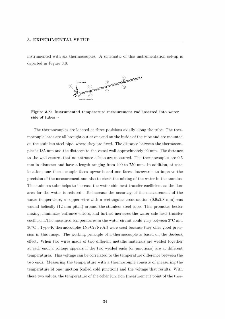
depicted in Figure 3.8.
Figure 3.8: Instrumented temperature measurement rod inserted into water
side of tubes -
The thermocouples are located at three positions axially along the tube. The ther-
mocouple leads are all brought out at one end on the inside of the tube and are mounted
on the stainless steel pipe, where they are fixed. The distance between the thermocou-
ples is 185 mm and the distance to the vessel wall approximately 92 mm. The distance
to the wall ensures that no entrance effects are measured. The thermocouples are 0.5
mm in diameter and have a length ranging from 400 to 750 mm. In addition, at each
location, one thermocouple faces upwards and one faces downwards to improve the
precision of the measurement and also to check the mixing of the water in the annulus.
The stainless tube helps to increase the water side heat transfer coefficient as the flow
area for the water is reduced. To increase the accuracy of the measurement of the
water temperature, a copper wire with a rectangular cross section (0.9x2.8 mm) was
wound helically (12 mm pitch) around the stainless steel tube. This promotes better
mixing, minimizes entrance effects, and further increases the water side heat transfer
coefficient.The measured temperatures in the water circuit could vary between 3◦C and
30◦C . Type-K thermocouples (Ni-Cr/Ni-Al) were used because they offer good preci-
sion in this range. The working principle of a thermocouple is based on the Seebeck
effect. When two wires made of two different metallic materials are welded together
at each end, a voltage appears if the two welded ends (or junctions) are at different
temperatures. This voltage can be correlated to the temperature difference between the
two ends. Measuring the temperature with a thermocouple consists of measuring the
temperature of one junction (called cold junction) and the voltage that results. With
these two values, the temperature of the other junction (measurement point of the ther-
34
3.3 Refrigerants
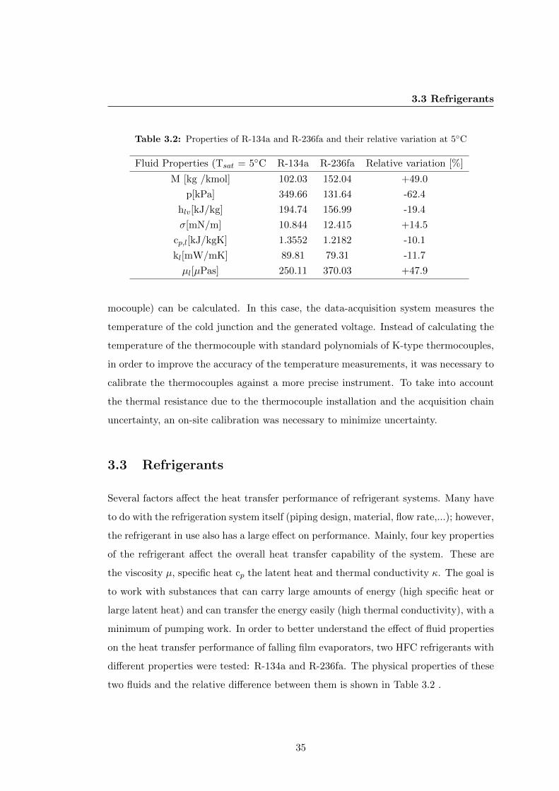
Table 3.2: Properties of R-134a and R-236fa and their relative variation at 5◦C
Fluid Properties (Tsat = 5◦C R-134a R-236fa Relative variation [%]
M [kg /kmol] 102.03 152.04 +49.0
p[kPa] 349.66 131.64 -62.4
hlv[kJ/kg] 194.74 156.99 -19.4
σ[mN/m] 10.844 12.415 +14.5
cp,l[kJ/kgK] 1.3552 1.2182 -10.1
kl[mW/mK] 89.81 79.31 -11.7
µl[µPas] 250.11 370.03 +47.9
mocouple) can be calculated. In this case, the data-acquisition system measures the
temperature of the cold junction and the generated voltage. Instead of calculating the
temperature of the thermocouple with standard polynomials of K-type thermocouples,
in order to improve the accuracy of the temperature measurements, it was necessary to
calibrate the thermocouples against a more precise instrument. To take into account
the thermal resistance due to the thermocouple installation and the acquisition chain
uncertainty, an on-site calibration was necessary to minimize uncertainty.
3.3 Refrigerants
Several factors affect the heat transfer performance of refrigerant systems. Many have
to do with the refrigeration system itself (piping design, material, flow rate,...); however,
the refrigerant in use also has a large effect on performance. Mainly, four key properties
of the refrigerant affect the overall heat transfer capability of the system. These are
the viscosity µ, specific heat cp the latent heat and thermal conductivity κ. The goal is
to work with substances that can carry large amounts of energy (high specific heat or
large latent heat) and can transfer the energy easily (high thermal conductivity), with a
minimum of pumping work. In order to better understand the effect of fluid properties
on the heat transfer performance of falling film evaporators, two HFC refrigerants with
different properties were tested: R-134a and R-236fa. The physical properties of these
two fluids and the relative difference between them is shown in Table 3.2 .
35
3. EXPERIMENTAL SETUP
3.4 Data reduction procedure
Using water inside the tubes to evaporate the refrigerant on the outside of the tubes,
the water undergoes a temperature change while the temperature of the evaporating
refrigerant remains constant. This produces a variation in the local heat flux as the
temperature difference between the water and the refrigerant decreases along the length
of the tubes. In other published studies outside of the LTCM laboratory, only the inlet
and outlet temperatures of the water have been measured. This means that all have
assumed a linear water temperature profile as a function of the tube length. Further-
more, this implies that a mean heat flux was applied to obtain a mean heat transfer
coefficient for each tube rather than axially local perimeter-averaged values. In this
study, the internally mounted thermocouples measuring the water temperature within
the tubes in the axial direction permit the determination of the water temperature
profile as a function of the distance along the tubes:
Twat = f(x) (3.1)
The local heat flux on the outside of the tube can be derived from the water tem-
perature profile as
qo =mcp,wat
πDo
dTwat
dx(3.2)
where m is the mass flow rate and cp,watis the isobaric specific heat of water. The
local overall heat transfer coefficient Uo can be calculated from the heat flux as
Uo =qo
Tsat − Twat(3.3)
with the saturation temperature of the refrigerant Tsat and the bulk temperature
of the water Twat. The evaporating-side heat transfer coefficient ho is obtained from:
ho =
[1
Uo− 1
hi
(Do
Di
)−Rw
]−1
(3.4)
where hi is the water side heat transfer coefficient and Rw is the thermal resistance
of the copper tube given by
Rw =Do
2κculn
(Dor
Di
)(3.5)
36
3.4 Data reduction procedure
Di is the inside diameter of the tube, Dor is the outside root diameter, and κCu is
the thermal conductivity of the tube material. The inside heat transfer coefficient hi is
obtained from the Gnielinski (1975) correlation with a corrective multiplier:
hi = Cihgni (3.6)
The determination of this corrective multiplier Ci, which includes influences of the
experimental setup, is described in Appendix A.
With the help of Equations (3.2) to (3.6), the axially local perimeter-averaged
heat transfer on the outside of the tube can be calculated from the measured water
temperature profile, the water mass flow rate, and the saturation temperature of the
refrigerant. For a given water temperature profile, the outside heat transfer coefficient
can be calculated at any location along the axis of the tube. However, in this study the
coefficient ho is only evaluated at the midpoint of every tube, where the most accurate
measurement can be made. The amount of liquid refrigerant evaporating on the outside
of one tube is derived from the local heat flux given by Equation (3.2) and the latent
heat hlv of the refrigerant. With the assumption that the liquid on the tube is at its
saturation condition, the mass flow of refrigerant evaporating locally on one tube is
calculated by an energy balance on a differential element as
(2Γbottom − 2Γtop)hlvdx = qoπDodx (3.7)
where 2Γ is the total mass flow rate on the tube per unit width and Γ is the flow
rate on one side of the tube per unit length of tube falling on top of the tube or leaving
at the bottom, respectively. With this definition, the film Reynolds number on the
tube is
Re =4Γ
µL(3.8)
For the measurements with liquid overfeed, the film Reynolds number of the liquid
arriving on the first tube is obtained from the measured mass flow rate (Coriolis mass
flow meter) and the tube length, assuming that the refrigerant is at saturation condi-
tions (it is subcooled less than 0.8K). The amount of liquid refrigerant evaporated on
the first tube calculated with Equation(3.7) is subtracted to obtain the film Reynolds
number at the bottom of the first tube. The film Reynolds number of the liquid falling
37
3. EXPERIMENTAL SETUP
on the second tube is set to the value leaving the first and so on. This means an ideal
one-dimension downward flow is assumed on the tube rows with all the liquid flowing
from one tube to the next without leaving the tube row. Thus, the mass flow rate per
unit width of the liquid falling onto the next tube in the array one side of the tube is
obtained by
Γtop,i = Γoverfeed −i−1∑n=1
qo,nπDo
2hLV(3.9)
where Γoverfeed is the amount of liquid from the liquid distributor per unit width
of tube and on one side of the tube.
38
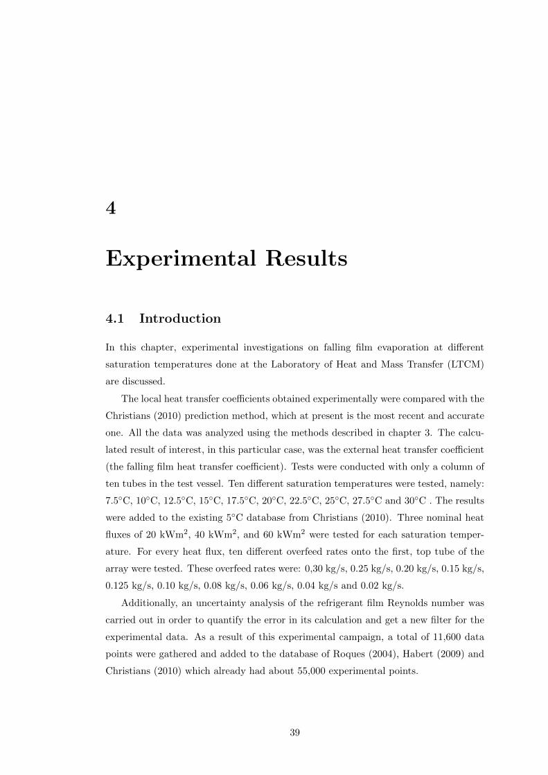
4
Experimental Results
4.1 Introduction
In this chapter, experimental investigations on falling film evaporation at different
saturation temperatures done at the Laboratory of Heat and Mass Transfer (LTCM)
are discussed.
The local heat transfer coefficients obtained experimentally were compared with the
Christians (2010) prediction method, which at present is the most recent and accurate
one. All the data was analyzed using the methods described in chapter 3. The calcu-
lated result of interest, in this particular case, was the external heat transfer coefficient
(the falling film heat transfer coefficient). Tests were conducted with only a column of
ten tubes in the test vessel. Ten different saturation temperatures were tested, namely:
7.5◦C, 10◦C, 12.5◦C, 15◦C, 17.5◦C, 20◦C, 22.5◦C, 25◦C, 27.5◦C and 30◦C . The results
were added to the existing 5◦C database from Christians (2010). Three nominal heat
fluxes of 20 kWm2, 40 kWm2, and 60 kWm2 were tested for each saturation temper-
ature. For every heat flux, ten different overfeed rates onto the first, top tube of the
array were tested. These overfeed rates were: 0,30 kg/s, 0.25 kg/s, 0.20 kg/s, 0.15 kg/s,
0.125 kg/s, 0.10 kg/s, 0.08 kg/s, 0.06 kg/s, 0.04 kg/s and 0.02 kg/s.
Additionally, an uncertainty analysis of the refrigerant film Reynolds number was
carried out in order to quantify the error in its calculation and get a new filter for the
experimental data. As a result of this experimental campaign, a total of 11,600 data
points were gathered and added to the database of Roques (2004), Habert (2009) and
Christians (2010) which already had about 55,000 experimental points.
39
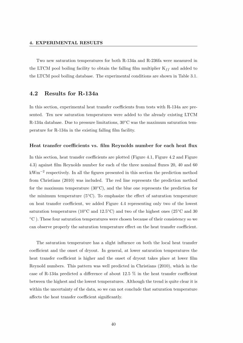
4. EXPERIMENTAL RESULTS
Two new saturation temperatures for both R-134a and R-236fa were measured in
the LTCM pool boiling facility to obtain the falling film multiplier Kff and added to
the LTCM pool boiling database. The experimental conditions are shown in Table 3.1.
4.2 Results for R-134a
In this section, experimental heat transfer coefficients from tests with R-134a are pre-
sented. Ten new saturation temperatures were added to the already existing LTCM
R-134a database. Due to pressure limitations, 30◦C was the maximum saturation tem-
perature for R-134a in the existing falling film facility.
Heat transfer coefficients vs. film Reynolds number for each heat flux
In this section, heat transfer coefficients are plotted (Figure 4.1, Figure 4.2 and Figure
4.3) against film Reynolds number for each of the three nominal fluxes 20, 40 and 60
kWm−2 respectively. In all the figures presented in this section the prediction method
from Christians (2010) was included. The red line represents the prediction method
for the maximum temperature (30◦C), and the blue one represents the prediction for
the minimum temperature (5◦C). To emphasize the effect of saturation temperature
on heat transfer coefficient, we added Figure 4.4 representing only two of the lowest
saturation temperatures (10◦C and 12.5◦C) and two of the highest ones (25◦C and 30
◦C ). These four saturation temperatures were chosen because of their consistency so we
can observe properly the saturation temperature effect on the heat transfer coefficient.
The saturation temperature has a slight influence on both the local heat transfer
coefficient and the onset of dryout. In general, at lower saturation temperatures the
heat transfer coefficient is higher and the onset of dryout takes place at lower film
Reynold numbers. This pattern was well predicted in Christians (2010), which in the
case of R-134a predicted a difference of about 12.5 % in the heat transfer coefficient
between the highest and the lowest temperatures. Although the trend is quite clear it is
within the uncertainty of the data, so we can not conclude that saturation temperature
affects the heat transfer coefficient significantly.
40
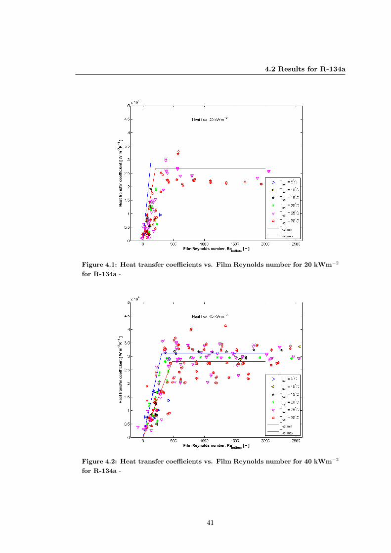
4.2 Results for R-134a
Figure 4.1: Heat transfer coefficients vs. Film Reynolds number for 20 kWm−2
for R-134a -
Figure 4.2: Heat transfer coefficients vs. Film Reynolds number for 40 kWm−2
for R-134a -
41
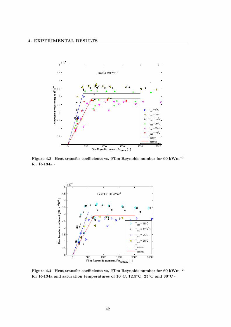
4. EXPERIMENTAL RESULTS
Figure 4.3: Heat transfer coefficients vs. Film Reynolds number for 60 kWm−2
for R-134a -
Figure 4.4: Heat transfer coefficients vs. Film Reynolds number for 60 kWm−2
for R-134a and saturation temperatures of 10◦C, 12.5◦C, 25◦C and 30◦C -
42
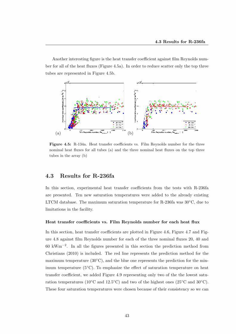
4.3 Results for R-236fa
Another interesting figure is the heat transfer coefficient against film Reynolds num-
ber for all of the heat fluxes (Figure 4.5a). In order to reduce scatter only the top three
tubes are represented in Figure 4.5b.
(a) (b)
Figure 4.5: R-134a. Heat transfer coefficients vs. Film Reynolds number for the three
nominal heat fluxes for all tubes (a) and the three nominal heat fluxes on the top three
tubes in the array (b)
4.3 Results for R-236fa
In this section, experimental heat transfer coefficients from the tests with R-236fa
are presented. Ten new saturation temperatures were added to the already existing
LTCM database. The maximum saturation temperature for R-236fa was 30◦C, due to
limitations in the facility.
Heat transfer coefficients vs. Film Reynolds number for each heat flux
In this section, heat transfer coefficients are plotted in Figure 4.6, Figure 4.7 and Fig-
ure 4.8 against film Reynolds number for each of the three nominal fluxes 20, 40 and
60 kWm−2. In all the figures presented in this section the prediction method from
Christians (2010) is included. The red line represents the prediction method for the
maximum temperature (30◦C), and the blue one represents the prediction for the min-
imum temperature (5◦C). To emphasize the effect of saturation temperature on heat
transfer coefficient, we added Figure 4.9 representing only two of the the lowest satu-
ration temperatures (10◦C and 12.5◦C) and two of the highest ones (25◦C and 30◦C).
These four saturation temperatures were chosen because of their consistency so we can
43
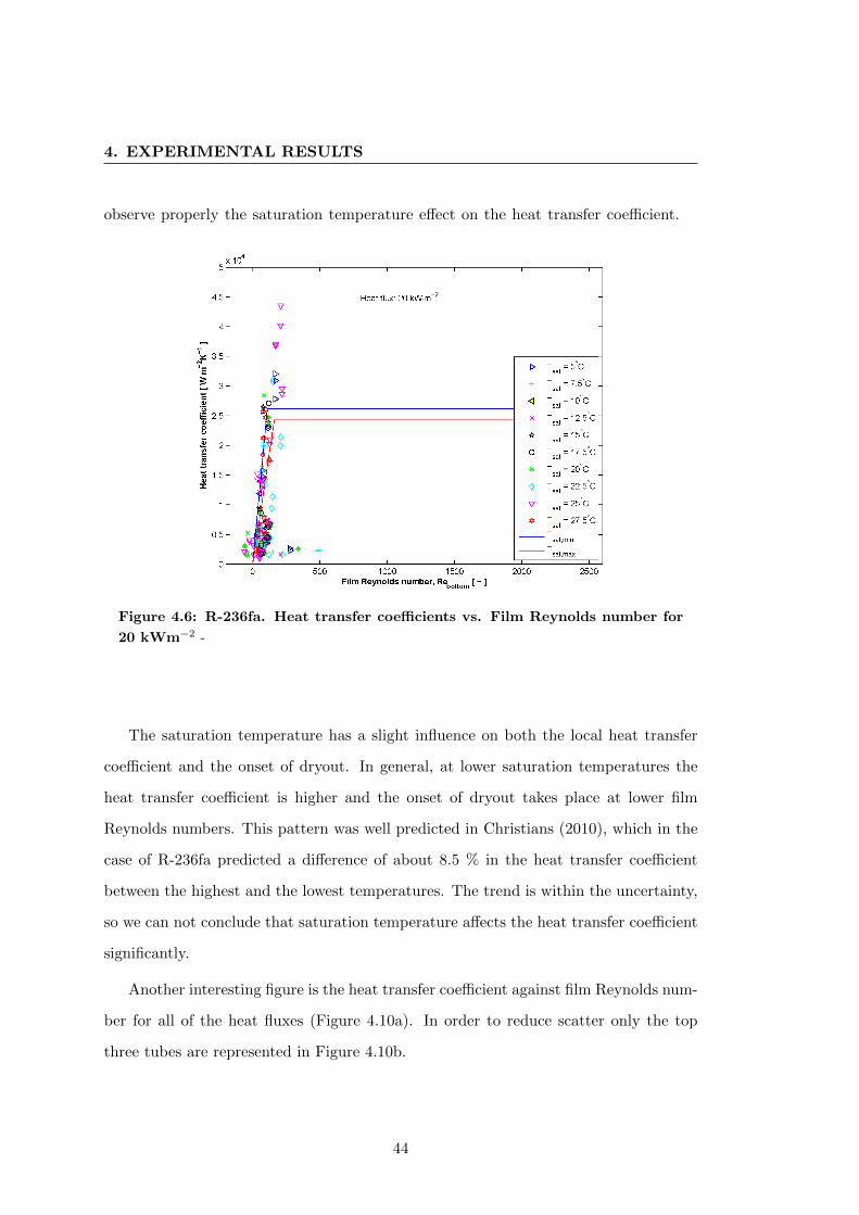
4. EXPERIMENTAL RESULTS
observe properly the saturation temperature effect on the heat transfer coefficient.
Figure 4.6: R-236fa. Heat transfer coefficients vs. Film Reynolds number for
20 kWm−2 -
The saturation temperature has a slight influence on both the local heat transfer
coefficient and the onset of dryout. In general, at lower saturation temperatures the
heat transfer coefficient is higher and the onset of dryout takes place at lower film
Reynolds numbers. This pattern was well predicted in Christians (2010), which in the
case of R-236fa predicted a difference of about 8.5 % in the heat transfer coefficient
between the highest and the lowest temperatures. The trend is within the uncertainty,
so we can not conclude that saturation temperature affects the heat transfer coefficient
significantly.
Another interesting figure is the heat transfer coefficient against film Reynolds num-
ber for all of the heat fluxes (Figure 4.10a). In order to reduce scatter only the top
three tubes are represented in Figure 4.10b.
44
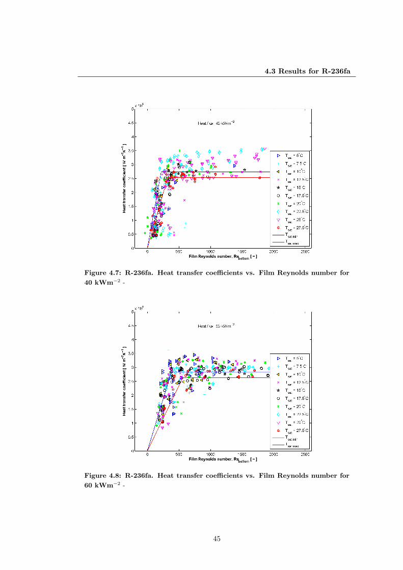
4.3 Results for R-236fa
Figure 4.7: R-236fa. Heat transfer coefficients vs. Film Reynolds number for
40 kWm−2 -
Figure 4.8: R-236fa. Heat transfer coefficients vs. Film Reynolds number for
60 kWm−2 -
45
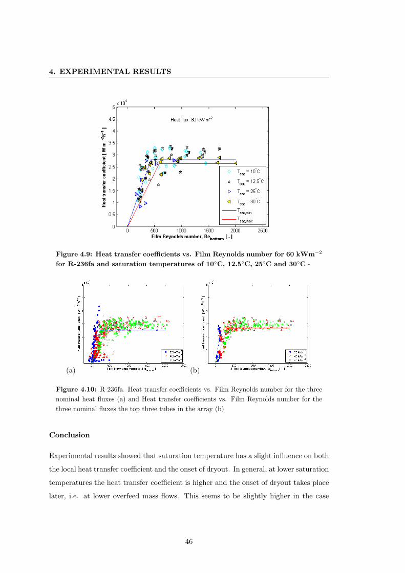
4. EXPERIMENTAL RESULTS
Figure 4.9: Heat transfer coefficients vs. Film Reynolds number for 60 kWm−2
for R-236fa and saturation temperatures of 10◦C, 12.5◦C, 25◦C and 30◦C -
(a) (b)
Figure 4.10: R-236fa. Heat transfer coefficients vs. Film Reynolds number for the three
nominal heat fluxes (a) and Heat transfer coefficients vs. Film Reynolds number for the
three nominal fluxes the top three tubes in the array (b)
Conclusion
Experimental results showed that saturation temperature has a slight influence on both
the local heat transfer coefficient and the onset of dryout. In general, at lower saturation
temperatures the heat transfer coefficient is higher and the onset of dryout takes place
later, i.e. at lower overfeed mass flows. This seems to be slightly higher in the case
46
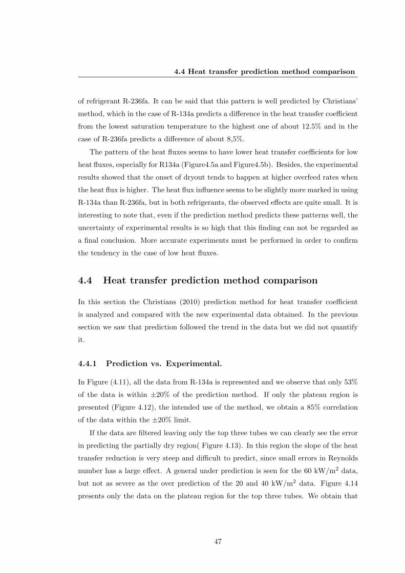
4.4 Heat transfer prediction method comparison
of refrigerant R-236fa. It can be said that this pattern is well predicted by Christians’
method, which in the case of R-134a predicts a difference in the heat transfer coefficient
from the lowest saturation temperature to the highest one of about 12.5% and in the
case of R-236fa predicts a difference of about 8,5%.
The pattern of the heat fluxes seems to have lower heat transfer coefficients for low
heat fluxes, especially for R134a (Figure4.5a and Figure4.5b). Besides, the experimental
results showed that the onset of dryout tends to happen at higher overfeed rates when
the heat flux is higher. The heat flux influence seems to be slightly more marked in using
R-134a than R-236fa, but in both refrigerants, the observed effects are quite small. It is
interesting to note that, even if the prediction method predicts these patterns well, the
uncertainty of experimental results is so high that this finding can not be regarded as
a final conclusion. More accurate experiments must be performed in order to confirm
the tendency in the case of low heat fluxes.
4.4 Heat transfer prediction method comparison
In this section the Christians (2010) prediction method for heat transfer coefficient
is analyzed and compared with the new experimental data obtained. In the previous
section we saw that prediction followed the trend in the data but we did not quantify
it.
4.4.1 Prediction vs. Experimental.
In Figure (4.11), all the data from R-134a is represented and we observe that only 53%
of the data is within ±20% of the prediction method. If only the plateau region is
presented (Figure 4.12), the intended use of the method, we obtain a 85% correlation
of the data within the ±20% limit.
If the data are filtered leaving only the top three tubes we can clearly see the error
in predicting the partially dry region( Figure 4.13). In this region the slope of the heat
transfer reduction is very steep and difficult to predict, since small errors in Reynolds
number has a large effect. A general under prediction is seen for the 60 kW/m2 data,
but not as severe as the over prediction of the 20 and 40 kW/m2 data. Figure 4.14
presents only the data on the plateau region for the top three tubes. We obtain that
47
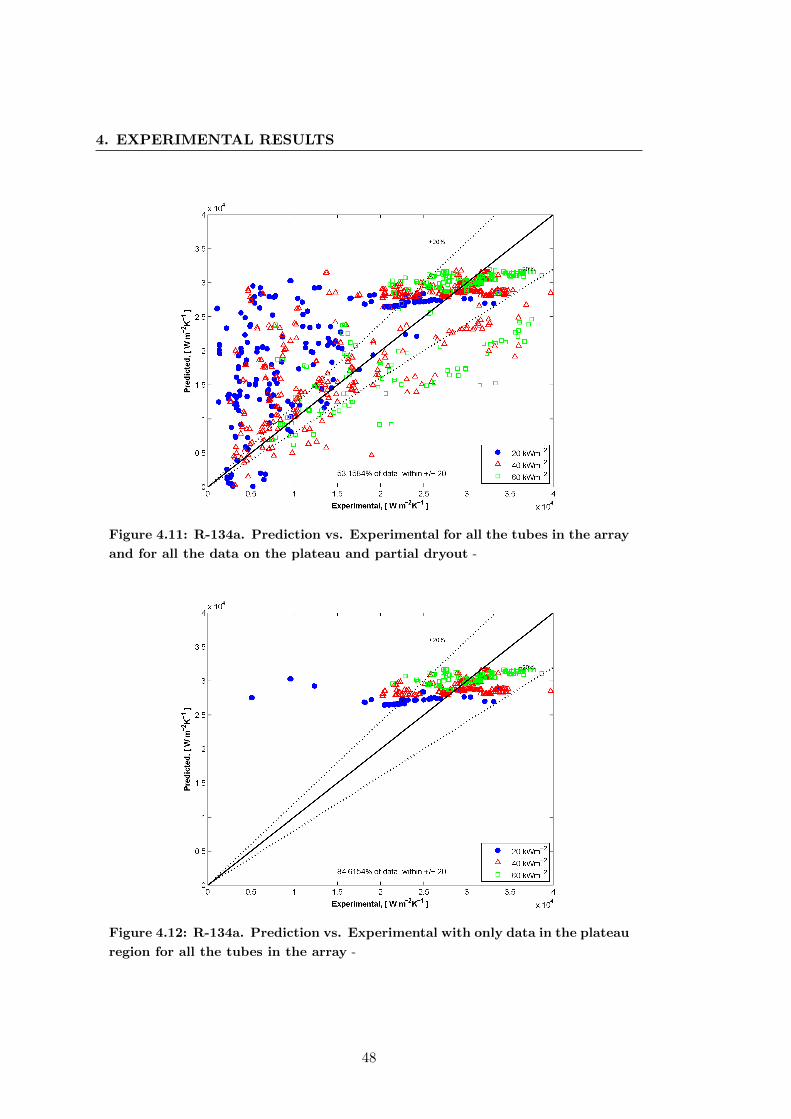
4. EXPERIMENTAL RESULTS
Figure 4.11: R-134a. Prediction vs. Experimental for all the tubes in the array
and for all the data on the plateau and partial dryout -
Figure 4.12: R-134a. Prediction vs. Experimental with only data in the plateau
region for all the tubes in the array -
48
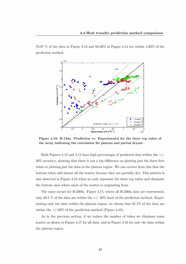
4.4 Heat transfer prediction method comparison
70.87 % of the data in Figure 4.13 and 94.36% in Figure 4.14 are within ±20% of the
prediction method.
Figure 4.13: R-134a. Prediction vs. Experimental for the three top tubes of
the array indicating the correlation for plateau and partial dryout -
Both Figures 4.12 and 4.14 have high percentages of predicted data within the +/-
20% accuracy, showing that there is not a big difference on plotting just the three first
tubes or plotting just the data in the plateau region. We can extract from this that the
bottom tubes add almost all the scatter because they are partially dry. This pattern is
also observed in Figure 4.13 when we only represent the three top tubes and eliminate
the bottom ones where most of the scatter is originating from.
The same occurs for R-236fa. Figure 4.15, where all R-236fa data are represented,
only 49.5 % of the data are within the +/- 20% limit of the prediction method. Repre-
senting only the data within the plateau region, we obtain that 85.1% of the data are
within the +/-20% of the prediction method (Figure 4.16).
As in the previous section, if we reduce the number of tubes we eliminate some
scatter as shown in Figure 4.17 for all data, and in Figure 4.18 for only the data within
the plateau region.
49
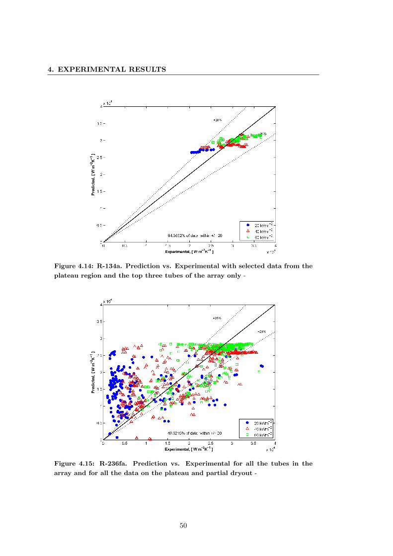
4. EXPERIMENTAL RESULTS
Figure 4.14: R-134a. Prediction vs. Experimental with selected data from the
plateau region and the top three tubes of the array only -
Figure 4.15: R-236fa. Prediction vs. Experimental for all the tubes in the
array and for all the data on the plateau and partial dryout -
50
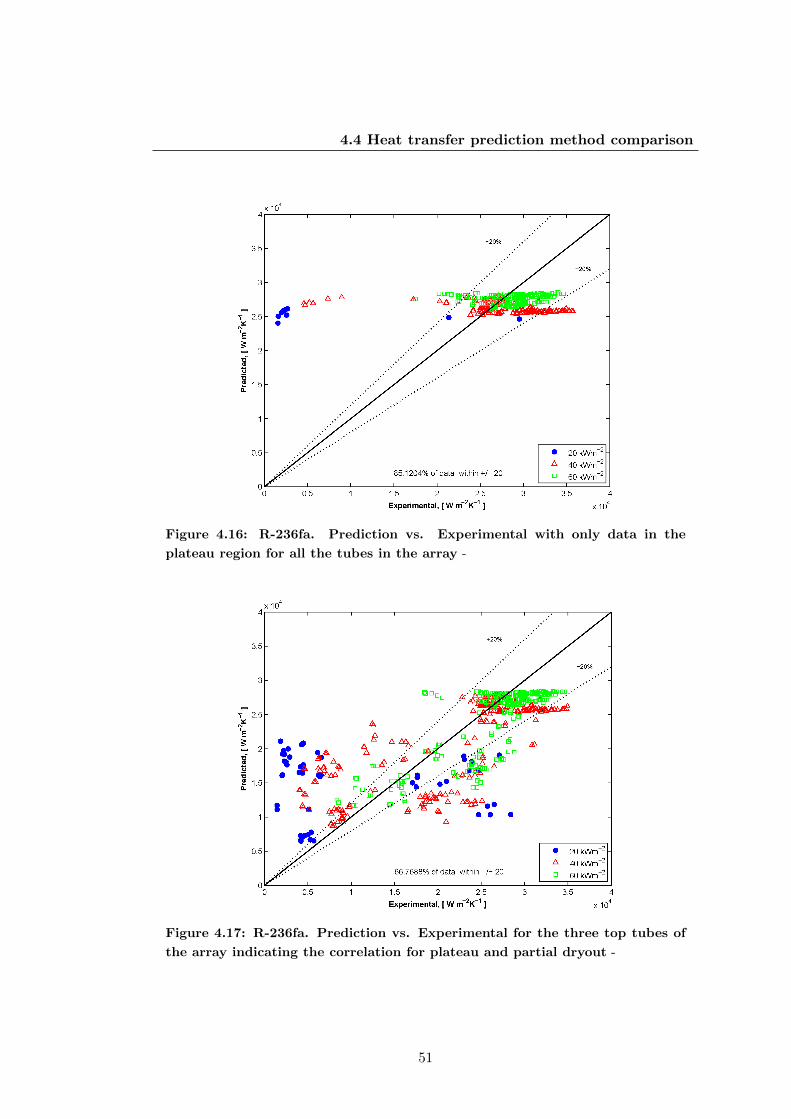
4.4 Heat transfer prediction method comparison
Figure 4.16: R-236fa. Prediction vs. Experimental with only data in the
plateau region for all the tubes in the array -
Figure 4.17: R-236fa. Prediction vs. Experimental for the three top tubes of
the array indicating the correlation for plateau and partial dryout -
51
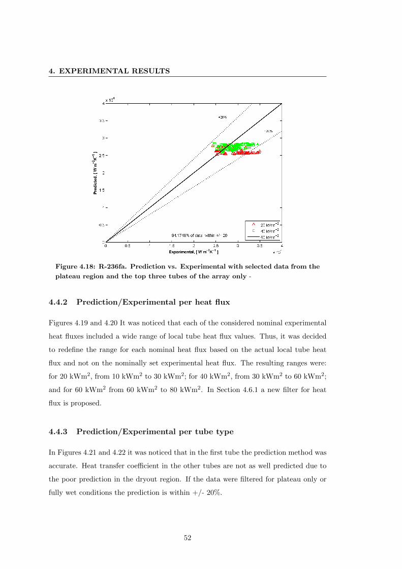
4. EXPERIMENTAL RESULTS
Figure 4.18: R-236fa. Prediction vs. Experimental with selected data from the
plateau region and the top three tubes of the array only -
4.4.2 Prediction/Experimental per heat flux
Figures 4.19 and 4.20 It was noticed that each of the considered nominal experimental
heat fluxes included a wide range of local tube heat flux values. Thus, it was decided
to redefine the range for each nominal heat flux based on the actual local tube heat
flux and not on the nominally set experimental heat flux. The resulting ranges were:
for 20 kWm2, from 10 kWm2 to 30 kWm2; for 40 kWm2, from 30 kWm2 to 60 kWm2;
and for 60 kWm2 from 60 kWm2 to 80 kWm2. In Section 4.6.1 a new filter for heat
flux is proposed.
4.4.3 Prediction/Experimental per tube type
In Figures 4.21 and 4.22 it was noticed that in the first tube the prediction method was
accurate. Heat transfer coefficient in the other tubes are not as well predicted due to
the poor prediction in the dryout region. If the data were filtered for plateau only or
fully wet conditions the prediction is within +/- 20%.
52
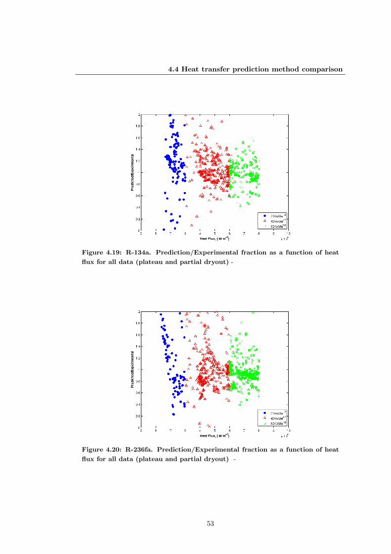
4.4 Heat transfer prediction method comparison
Figure 4.19: R-134a. Prediction/Experimental fraction as a function of heat
flux for all data (plateau and partial dryout) -
Figure 4.20: R-236fa. Prediction/Experimental fraction as a function of heat
flux for all data (plateau and partial dryout) -
53
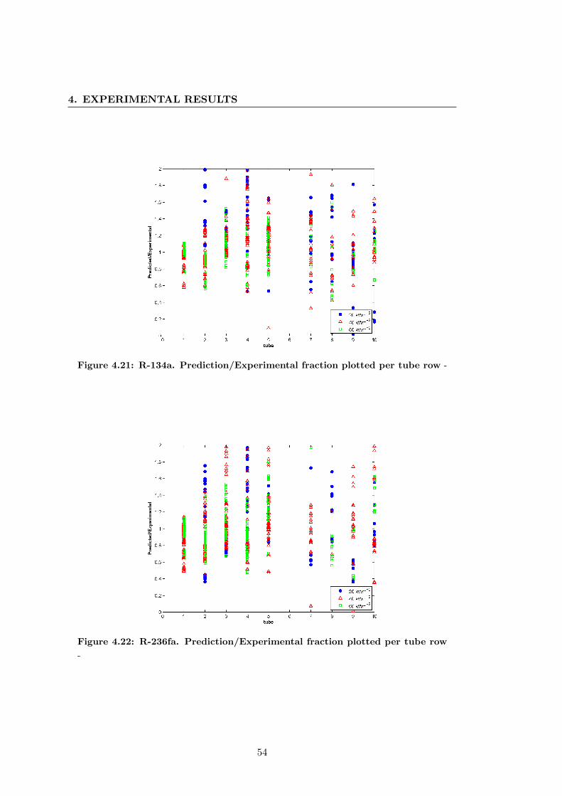
4. EXPERIMENTAL RESULTS
Figure 4.21: R-134a. Prediction/Experimental fraction plotted per tube row -
Figure 4.22: R-236fa. Prediction/Experimental fraction plotted per tube row
-
54
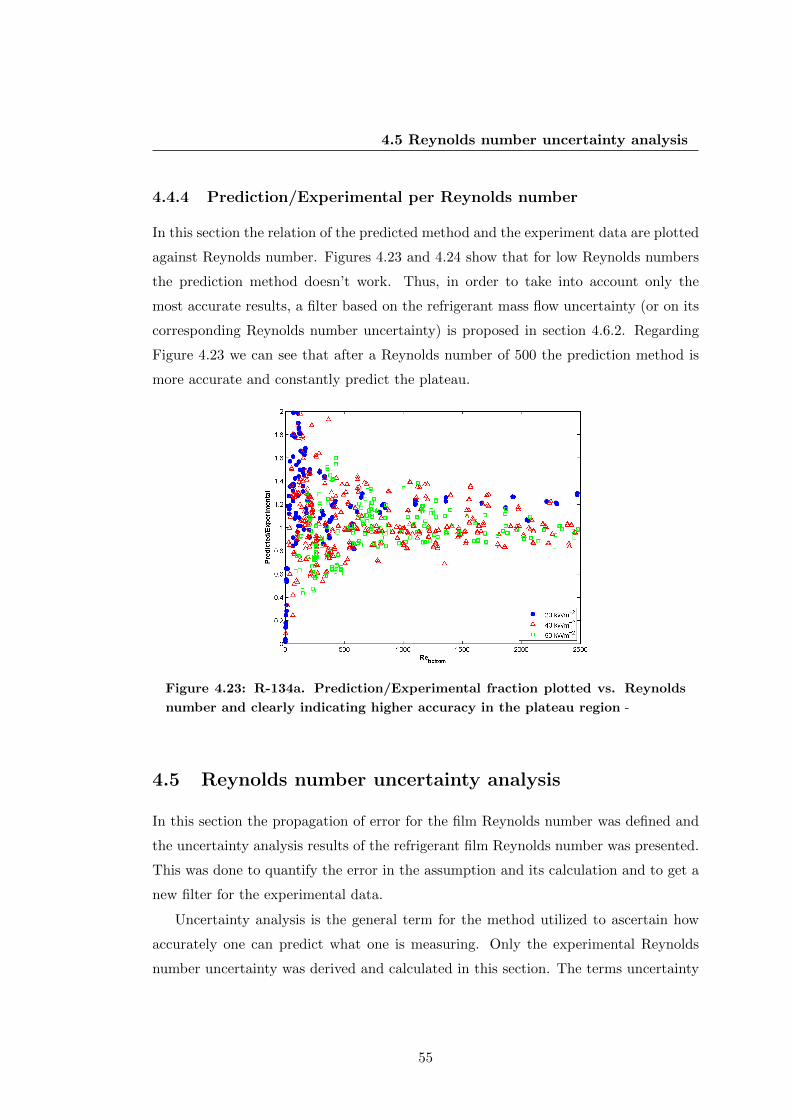
4.5 Reynolds number uncertainty analysis
4.4.4 Prediction/Experimental per Reynolds number
In this section the relation of the predicted method and the experiment data are plotted
against Reynolds number. Figures 4.23 and 4.24 show that for low Reynolds numbers
the prediction method doesn’t work. Thus, in order to take into account only the
most accurate results, a filter based on the refrigerant mass flow uncertainty (or on its
corresponding Reynolds number uncertainty) is proposed in section 4.6.2. Regarding
Figure 4.23 we can see that after a Reynolds number of 500 the prediction method is
more accurate and constantly predict the plateau.
Figure 4.23: R-134a. Prediction/Experimental fraction plotted vs. Reynolds
number and clearly indicating higher accuracy in the plateau region -
4.5 Reynolds number uncertainty analysis
In this section the propagation of error for the film Reynolds number was defined and
the uncertainty analysis results of the refrigerant film Reynolds number was presented.
This was done to quantify the error in the assumption and its calculation and to get a
new filter for the experimental data.
Uncertainty analysis is the general term for the method utilized to ascertain how
accurately one can predict what one is measuring. Only the experimental Reynolds
number uncertainty was derived and calculated in this section. The terms uncertainty
55
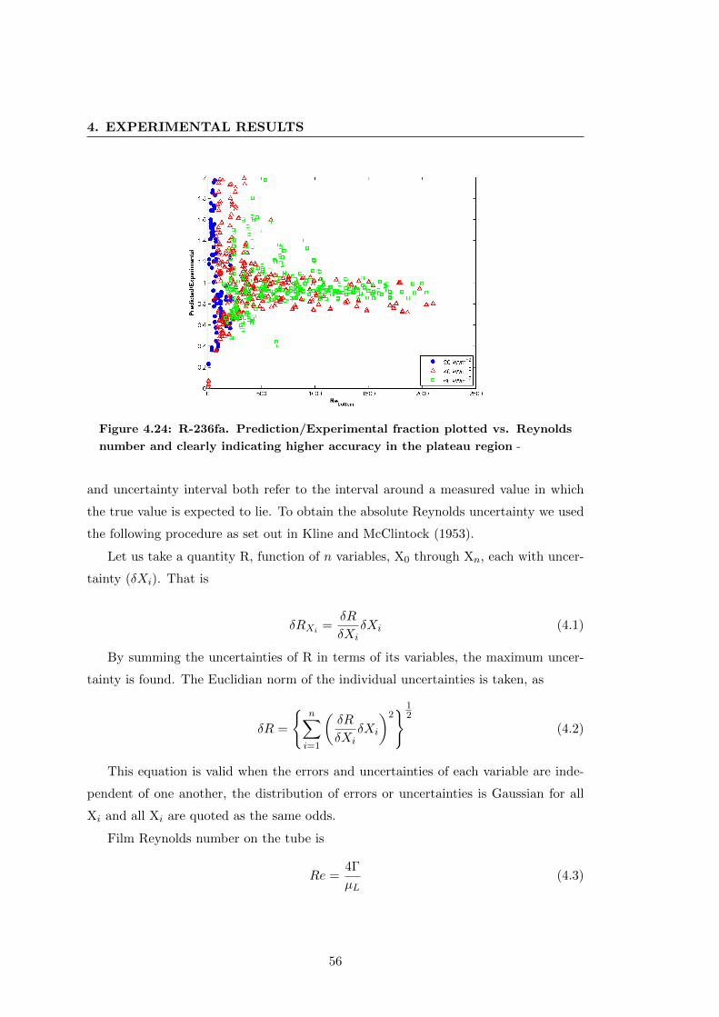
4. EXPERIMENTAL RESULTS
Figure 4.24: R-236fa. Prediction/Experimental fraction plotted vs. Reynolds
number and clearly indicating higher accuracy in the plateau region -
and uncertainty interval both refer to the interval around a measured value in which
the true value is expected to lie. To obtain the absolute Reynolds uncertainty we used
the following procedure as set out in Kline and McClintock (1953).
Let us take a quantity R, function of n variables, X0 through Xn, each with uncer-
tainty (δXi). That is
δRXi =δR
δXiδXi (4.1)
By summing the uncertainties of R in terms of its variables, the maximum uncer-
tainty is found. The Euclidian norm of the individual uncertainties is taken, as
δR =
{n∑
i=1
(δR
δXiδXi
)2}1
2
(4.2)
This equation is valid when the errors and uncertainties of each variable are inde-
pendent of one another, the distribution of errors or uncertainties is Gaussian for all
Xi and all Xi are quoted as the same odds.
Film Reynolds number on the tube is
Re =4Γ
µL(4.3)
56
4.5 Reynolds number uncertainty analysis
For the measurements with liquid overfeed, the film Reynolds number of the liquid
arriving on the first tube is obtained from the measured mass flow rate (Coriolis mass
flow meter). The amount of liquid refrigerant evaporated on the first tube is subtracted
to obtain the film Reynolds number at the bottom of the first tube. The film Reynolds
number of the liquid falling on the second tube is set to the value leaving the first and
so on. This means an ideal one-dimension downward flow is assumed on the tube rows
with all the liquid flowing from one tube to the next without leaving the tube row.
Thus, the mass flow rate per unit length of the liquid falling onto the next tube in the
array on one side of the tube is obtained by
Γtop,i+1 = Γi −n∑
i=1
qo,iπDo
2hLV(4.4)
where Γi is the amount of liquid from the liquid distributor per unit width of tube
and on one side of the tube.
From 4.3 the uncertainty in Re is
δRe =
((δRe
δΓδΓ
)2
+
(δRe
δµLδµL
)2)1
2
(4.5)
The partial derivatives are
δRe
δΓ=
4
µL(4.6)
δRe
δµL= −4Γ
µ2L(4.7)
The total uncertainty for δµL was obtained by Christians (2010) and was found to
be
δµL = 1.09% (4.8)
In order to obtain δΓ we used
Γn+i = Γn −qo,nπDo
2hLV(4.9)
Then the uncertainty in δΓn+i is
57
4. EXPERIMENTAL RESULTS
δΓn+i =
((δΓn+1
δΓnδΓn
)2
+
(δΓn+1
δqoδqo
)2
+
(δΓn+1
δhLVδhLV
)2)1
2
(4.10)
and the partial derivatives in terms of its components are
δΓn+1
δΓn= 1 (4.11)
δΓn+1
δqo= − πDo
2hLV(4.12)
δΓn+1
δhLV= +
qoπDo
2h2LV(4.13)
The uncertainty on the local heat flux (δqo) and δ hLV were obtained in Christians
(2010).
Equation 4.14 shows us the flow rate on one side of the tube per unit length
Γn =m
L(4.14)
The uncertainty in the flow rate is
δΓn =
∣∣∣∣δΓn
δmδm
∣∣∣∣ (4.15)
and the partial derivative isδΓn
δm=
1
L(4.16)
A Coriolis mass flow meter is installed in the refrigerant circuit. The uncertainty
in the measurement is provided by the manufacturer using the following equation:
δm/m ≤ ±(0.15 + S/m)% (4.17)
where S is a constant depending on the mass flow meter. For the units from 0 to
0,167 kg/s we have S=8.3 10−4 kg/s.
The relative uncertainty (δRe/Rebottom(%)) and the absolute uncertainty (δRe)
were both used for the results presentation.
The relative uncertainty film Reynolds number was represented in Figure 4.25
against the film Reynolds number and against each of the ten tubes in Figure 4.26. The
58
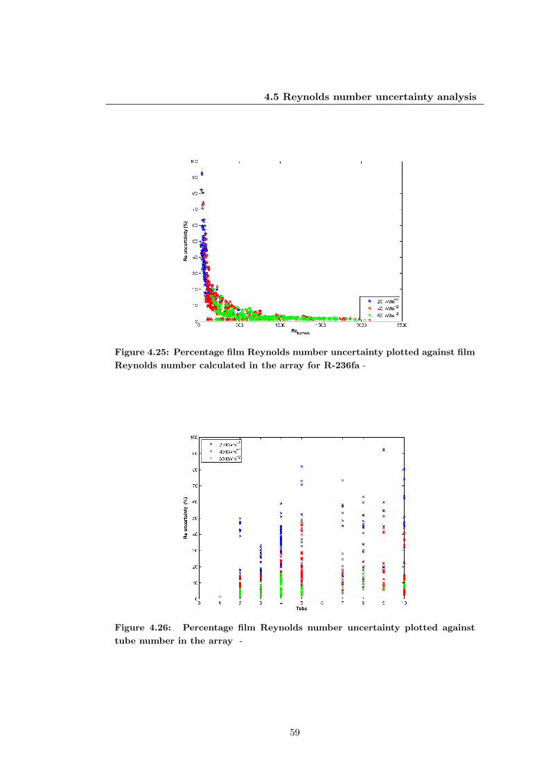
4.5 Reynolds number uncertainty analysis
Figure 4.25: Percentage film Reynolds number uncertainty plotted against film
Reynolds number calculated in the array for R-236fa -
Figure 4.26: Percentage film Reynolds number uncertainty plotted against
tube number in the array -
59
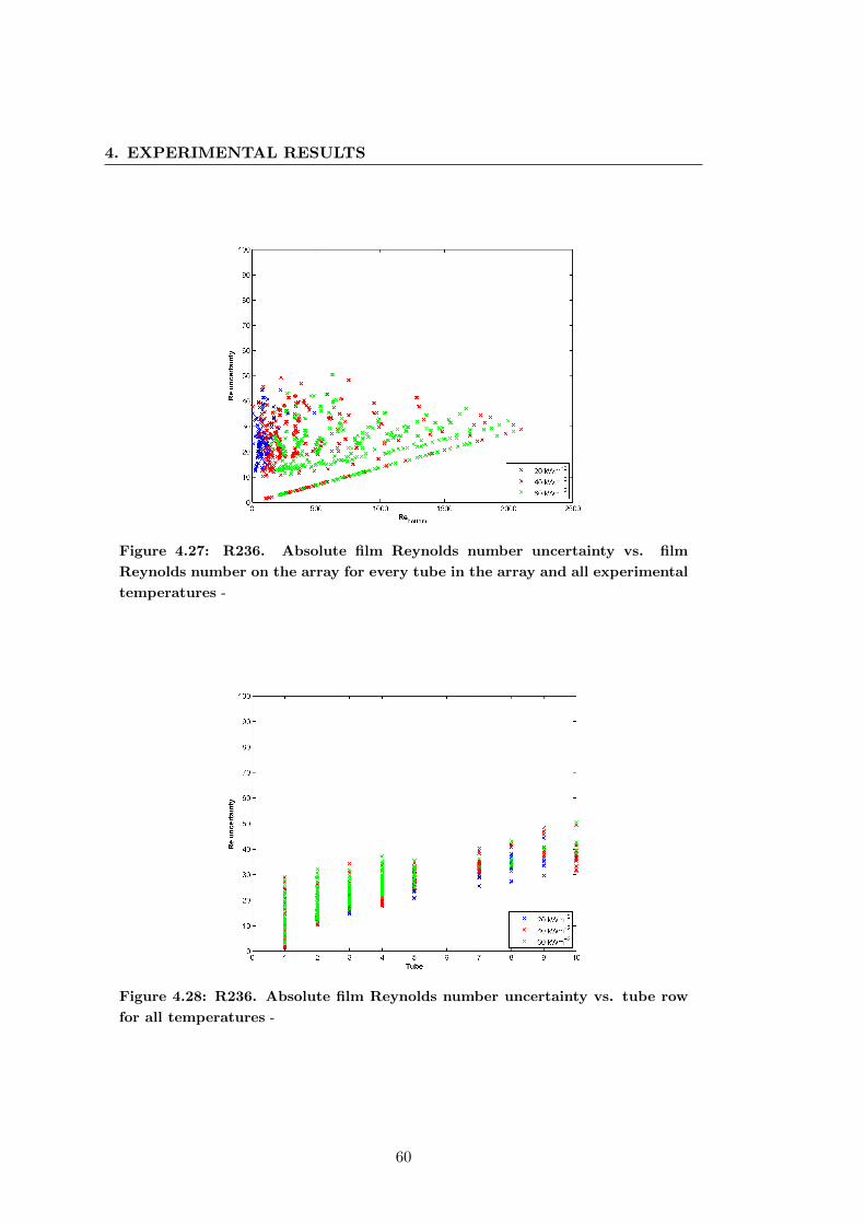
4. EXPERIMENTAL RESULTS
Figure 4.27: R236. Absolute film Reynolds number uncertainty vs. film
Reynolds number on the array for every tube in the array and all experimental
temperatures -
Figure 4.28: R236. Absolute film Reynolds number uncertainty vs. tube row
for all temperatures -
60
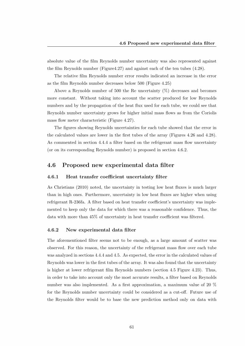
4.6 Proposed new experimental data filter
absolute value of the film Reynolds number uncertainty was also represented against
the film Reynolds number (Figure4.27) and against each of the ten tubes (4.28).
The relative film Reynolds number error results indicated an increase in the error
as the film Reynolds number decreases below 500 (Figure 4.25)
Above a Reynolds number of 500 the Re uncertainty (%) decreases and becomes
more constant. Without taking into account the scatter produced for low Reynolds
numbers and by the propagation of the heat flux used for each tube, we could see that
Reynolds number uncertainty grows for higher initial mass flows as from the Coriolis
mass flow meter characteristic (Figure 4.27).
The figures showing Reynolds uncertainties for each tube showed that the error in
the calculated values are lower in the first tubes of the array (Figures 4.26 and 4.28).
As commented in section 4.4.4 a filter based on the refrigerant mass flow uncertainty
(or on its corresponding Reynolds number) is proposed in section 4.6.2.
4.6 Proposed new experimental data filter
4.6.1 Heat transfer coefficient uncertainty filter
As Christians (2010) noted, the uncertainty in testing low heat fluxes is much larger
than in high ones. Furthermore, uncertainty in low heat fluxes are higher when using
refrigerant R-236fa. A filter based on heat transfer coefficient’s uncertainty was imple-
mented to keep only the data for which there was a reasonable confidence. Thus, the
data with more than 45% of uncertainty in heat transfer coefficient was filtered.
4.6.2 New experimental data filter
The aforementioned filter seems not to be enough, as a large amount of scatter was
observed. For this reason, the uncertainty of the refrigerant mass flow over each tube
was analyzed in sections 4.4.4 and 4.5. As expected, the error in the calculated values of
Reynolds was lower in the first tubes of the array. It was also found that the uncertainty
is higher at lower refrigerant film Reynolds numbers (section 4.5 Figure 4.23). Thus,
in order to take into account only the most accurate results, a filter based on Reynolds
number was also implemented. As a first approximation, a maximum value of 20 %
for the Reynolds number uncertainty could be considered as a cut-off. Future use of
the Reynolds filter would be to base the new prediction method only on data with
61
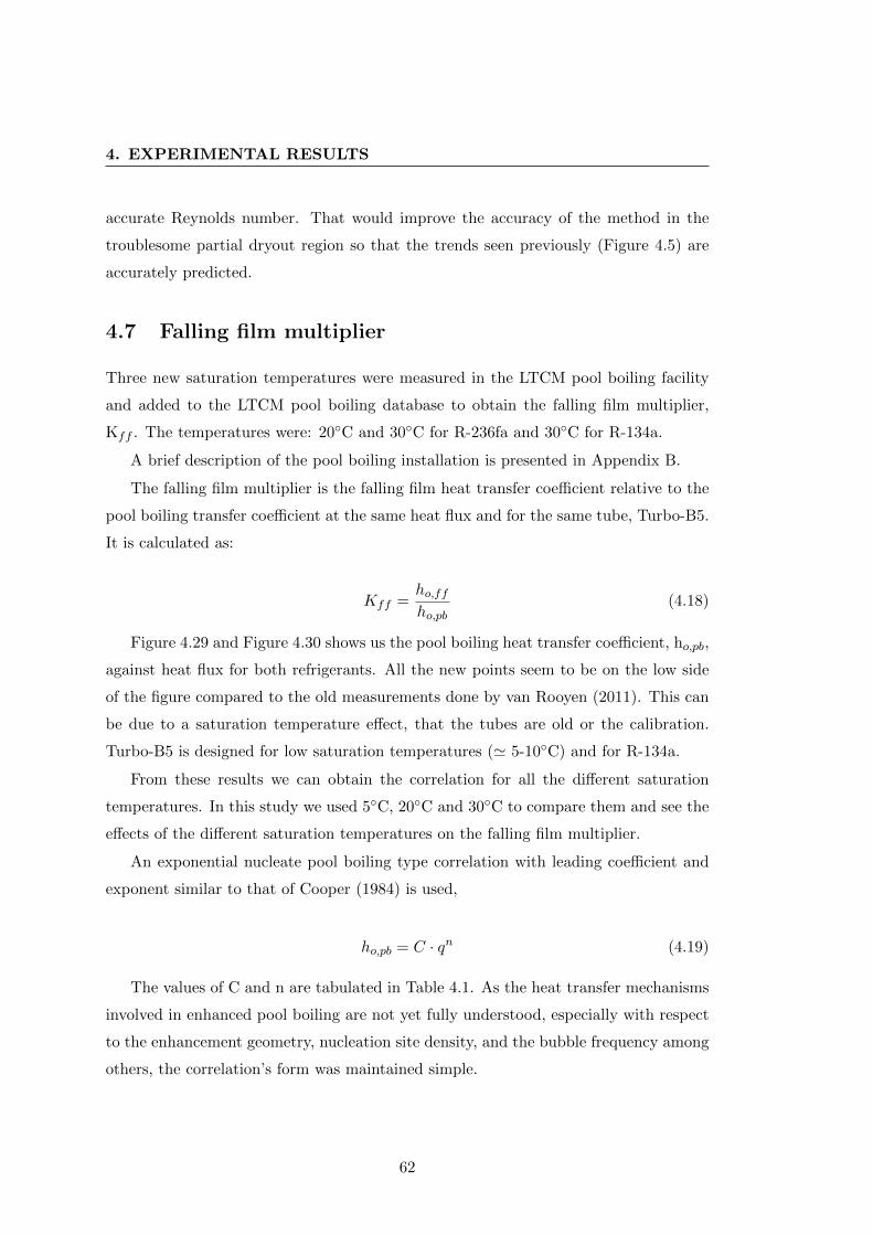
4. EXPERIMENTAL RESULTS
accurate Reynolds number. That would improve the accuracy of the method in the
troublesome partial dryout region so that the trends seen previously (Figure 4.5) are
accurately predicted.
4.7 Falling film multiplier
Three new saturation temperatures were measured in the LTCM pool boiling facility
and added to the LTCM pool boiling database to obtain the falling film multiplier,
Kff . The temperatures were: 20◦C and 30◦C for R-236fa and 30◦C for R-134a.
A brief description of the pool boiling installation is presented in Appendix B.
The falling film multiplier is the falling film heat transfer coefficient relative to the
pool boiling transfer coefficient at the same heat flux and for the same tube, Turbo-B5.
It is calculated as:
Kff =ho,ffho,pb
(4.18)
Figure 4.29 and Figure 4.30 shows us the pool boiling heat transfer coefficient, ho,pb,
against heat flux for both refrigerants. All the new points seem to be on the low side
of the figure compared to the old measurements done by van Rooyen (2011). This can
be due to a saturation temperature effect, that the tubes are old or the calibration.
Turbo-B5 is designed for low saturation temperatures (' 5-10◦C) and for R-134a.
From these results we can obtain the correlation for all the different saturation
temperatures. In this study we used 5◦C, 20◦C and 30◦C to compare them and see the
effects of the different saturation temperatures on the falling film multiplier.
An exponential nucleate pool boiling type correlation with leading coefficient and
exponent similar to that of Cooper (1984) is used,
ho,pb = C · qn (4.19)
The values of C and n are tabulated in Table 4.1. As the heat transfer mechanisms
involved in enhanced pool boiling are not yet fully understood, especially with respect
to the enhancement geometry, nucleation site density, and the bubble frequency among
others, the correlation’s form was maintained simple.
62
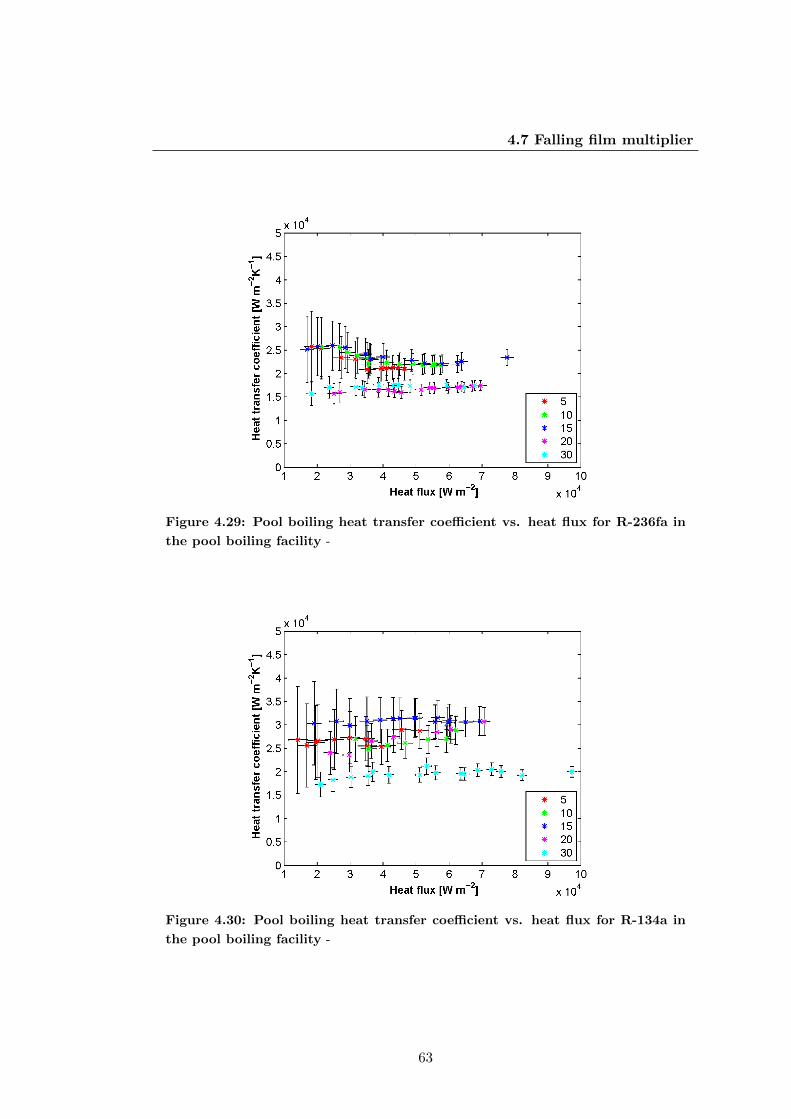
4.7 Falling film multiplier
Figure 4.29: Pool boiling heat transfer coefficient vs. heat flux for R-236fa in
the pool boiling facility -
Figure 4.30: Pool boiling heat transfer coefficient vs. heat flux for R-134a in
the pool boiling facility -
63
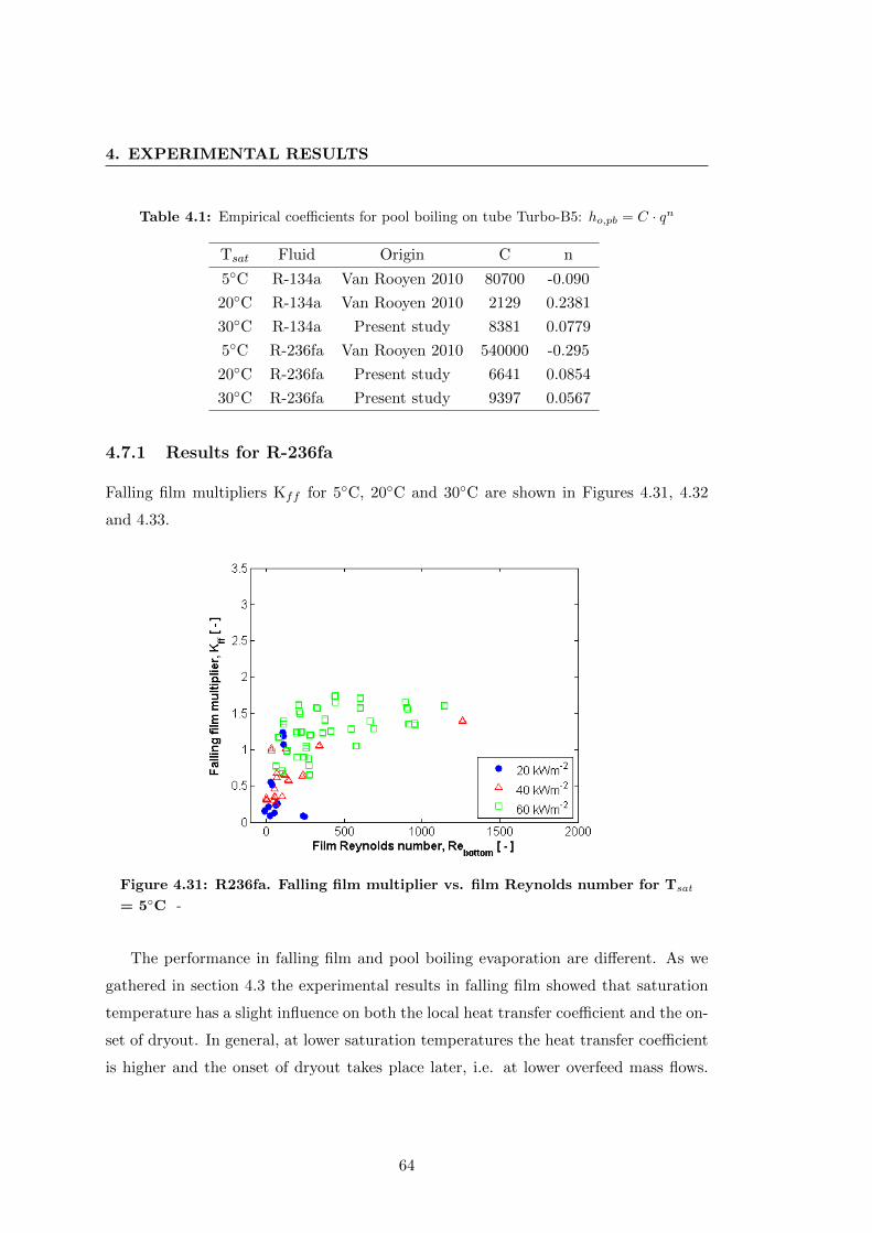
4. EXPERIMENTAL RESULTS
Table 4.1: Empirical coefficients for pool boiling on tube Turbo-B5: ho,pb = C · qn
Tsat Fluid Origin C n
5◦C R-134a Van Rooyen 2010 80700 -0.090
20◦C R-134a Van Rooyen 2010 2129 0.2381
30◦C R-134a Present study 8381 0.0779
5◦C R-236fa Van Rooyen 2010 540000 -0.295
20◦C R-236fa Present study 6641 0.0854
30◦C R-236fa Present study 9397 0.0567
4.7.1 Results for R-236fa
Falling film multipliers Kff for 5◦C, 20◦C and 30◦C are shown in Figures 4.31, 4.32
and 4.33.
Figure 4.31: R236fa. Falling film multiplier vs. film Reynolds number for Tsat
= 5◦C -
The performance in falling film and pool boiling evaporation are different. As we
gathered in section 4.3 the experimental results in falling film showed that saturation
temperature has a slight influence on both the local heat transfer coefficient and the on-
set of dryout. In general, at lower saturation temperatures the heat transfer coefficient
is higher and the onset of dryout takes place later, i.e. at lower overfeed mass flows.
64
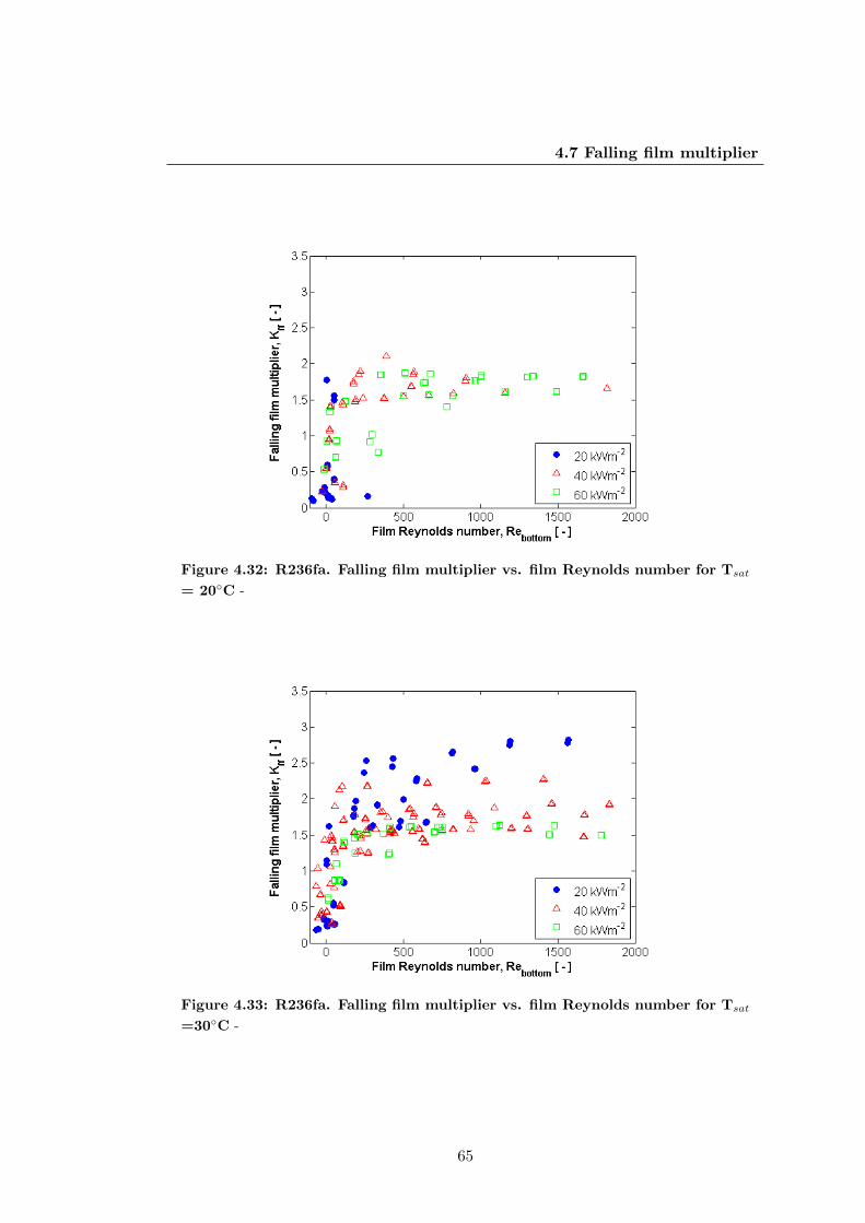
4.7 Falling film multiplier
Figure 4.32: R236fa. Falling film multiplier vs. film Reynolds number for Tsat
= 20◦C -
Figure 4.33: R236fa. Falling film multiplier vs. film Reynolds number for Tsat
=30◦C -
65
4. EXPERIMENTAL RESULTS
This effect would have decreased the falling film multiplier Kff in the hypothetical case
of pool boiling heat transfer coefficient remaining the same. Instead of decreasing, the
falling film multiplier increases for higher temperatures as shown in the Figures 4.31,
4.32 and 4.33 due to the low pool boiling heat transfer coefficient for 20◦C and 30◦C. As
observed in Figure 4.29, for 5◦C we obtain a ho,pb of ' 23500 Wm−2K−1 and the ho,pb
for 20◦C and 30◦C is only ' 17000 Wm−2K−1 and ' 16000 Wm−2K−1, respectively.
Therefore the pool boiling performance drops significantly with saturation temper-
ature while the falling film performance remains relatively high resulting in an increase
in Kff with saturation temperature.
4.7.2 Results for R-134a
Falling film multipliers Kff for 5◦C, 20◦C and 30◦C are shown in Figures 4.34, 4.35
and 4.36 for R-134a.
For R-134a the falling film evaporative heat transfer is '1.25 times more efficient
than pool boiling for 5◦C, same efficiency for 20◦C and '1.4 times more efficient than
pool boiling for 30◦C. The decrease in the falling film multiplier for T= 20◦C with
respect to T= 5◦C can be due that the correlation for 20◦C was done by van Rooyen
(2011) when the tube was new so it performed better and gave us a higher pool boiling
heat transfer coefficient. Thus, the Kff is lower.
The increase in the falling film multiplier for T= 30◦C is due to the low pool boiling
heat transfer coefficient for this temperature and this refrigerant. Whereas for 5◦C we
obtain a ho,pb of ' 27000 Wm−2K−1, the ho,pb for 30◦C is only ' 19000 Wm−2K−1.
We can conclude that there are two competing temperature effects that affect Kff .
When increasing the saturation temperature there is an observed decrease (inside un-
certainty) of the falling film heat transfer coefficient which decreases Kff . On the
other hand, pool boiling heat transfer coefficient is also decreased for higher satura-
tion temperatures so this increases the Kff . In our study, the pool boiling saturation
temperature effect is higher than the falling film saturation temperature effect so Kff
increases when temperature increases.
66
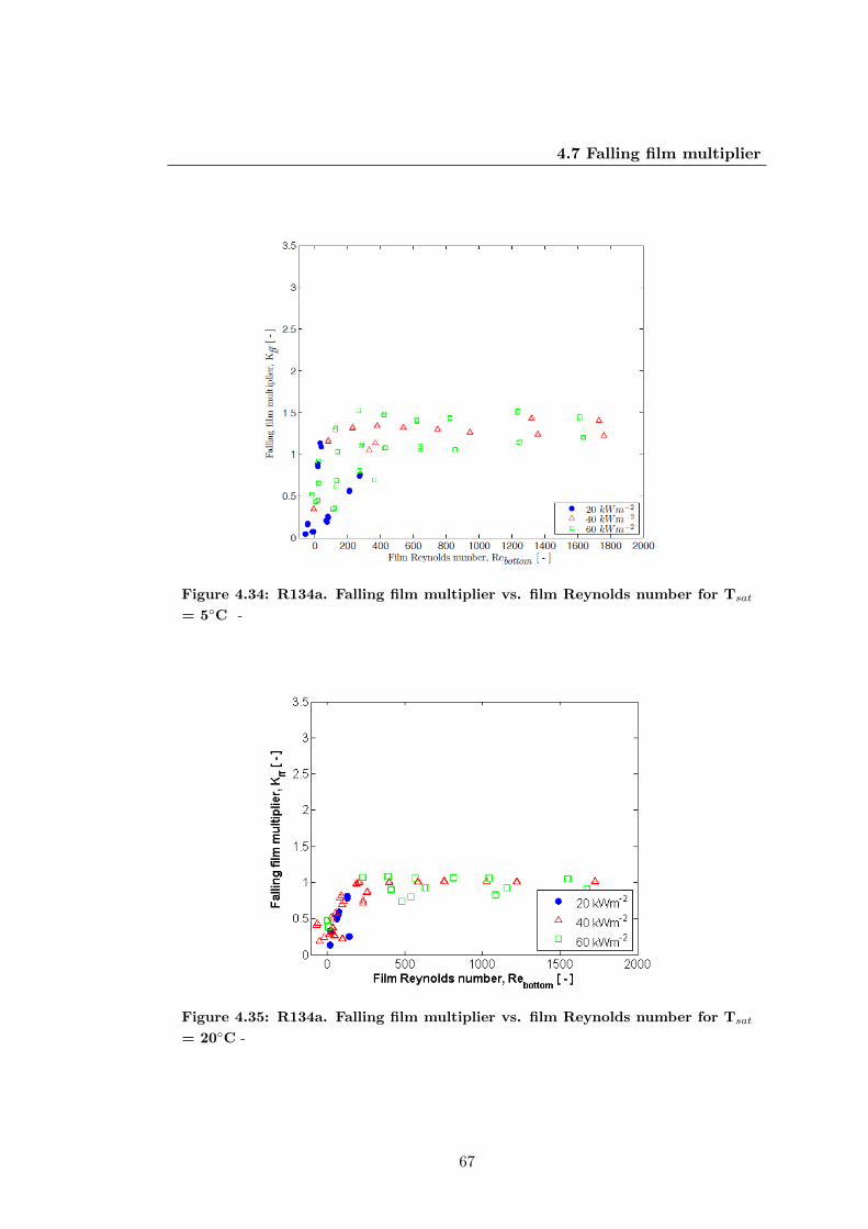
4.7 Falling film multiplier
Figure 4.34: R134a. Falling film multiplier vs. film Reynolds number for Tsat
= 5◦C -
Figure 4.35: R134a. Falling film multiplier vs. film Reynolds number for Tsat
= 20◦C -
67
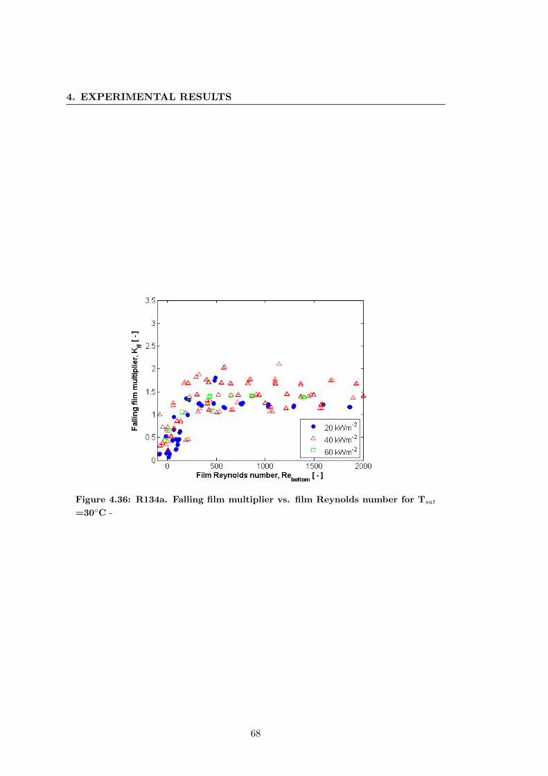
4. EXPERIMENTAL RESULTS
Figure 4.36: R134a. Falling film multiplier vs. film Reynolds number for Tsat
=30◦C -
68
5
Conclusion
Accurate values of local heat transfer coefficients on a tube array for different saturation
temperatures were obtained. Up to 30◦C saturation temperature for R-134a and R-
236fa was tested for three heat fluxes on a single column of tubes resulting in 11,600
new data points for the LTCM falling film database. Pool boiling experiments were
performed in order to obtain the falling film multiplier Kff . Three new saturation
temperatures for R-134a and R-236fa were measured in the LTCM pool boiling facility
and added to the LTCM Pool boiling database.
The falling film heat transfer coefficients obtained experimentally compared well
with Christians (2010) which in the case of R-134a predicted a difference of about 12.5 %
in the heat transfer coefficient between the highest (30◦C) and the lowest temperatures
(5◦C). It was found that at lower saturation temperatures the heat transfer coefficient
was higher and the onset of dryout takes place at higher film Reynolds numbers.
The tube had lower heat transfer coefficients for low heat fluxes in falling film.
The onset of dryout tended to happen at higher overfeed rates when the heat flux was
higher. The heat flux influence seemed to be slightly more marked when using R-134a
than R-236fa. It was interesting to note that, even if the prediction method predicts
these patterns well, the uncertainty of experimental results was very high especially at
low heat fluxes. More accurate experiments should be performed in order to confirm
the tendency. It was decided to redefine the range for each nominal heat flux based on
the actual local tube heat flux and not on the nominally set experimental heat flux.
During this study, it was noticed that the heat transfer prediction method was
not accurate for low Reynolds numbers. In this region the slope of the heat transfer
69
5. CONCLUSION
reduction was very steep and difficult to predict, since small errors in Reynolds number
had a large effect in heat transfer coefficient. A general under prediction was seen for
the 60 kW/m2 data and over prediction for 40 kW/m2 and 20 kW/m2.
Therefore, the propagation of error for the film Reynolds number was defined to
quantify the error in the assumption and its calculation and to get a new filter for
the experimental data. The future use of the Reynolds filter would be to base new
prediction methods only on data with accurate Reynolds numbers. That would improve
the accuracy of the method in the troublesome partial dryout region.
All the new pool boiling data points tested in the lab were lower compared to the
old measurements done by van Rooyen (2011). This could be due to a saturation
temperature effect, that the tubes were old (oxidized), the calibration or because the
Turbo-B5 tube was designed for low saturation temperatures (5◦C-15◦C). An exponen-
tial nucleate pool boiling type correlation with leading coefficient and exponent was
used to obtain the pool boiling heat transfer coefficient.
After obtaining Kff for the different saturation temperatures we concluded that
there are two competing temperature effects that affect Kff . When increasing the sat-
uration temperature there was an observed decrease (inside uncertainty) of the falling
film heat transfer coefficient which decreased Kff . On the other hand, pool boiling
heat transfer coefficients were also decreasing for higher saturation temperatures so
this increased the Kff . In this study, the pool boiling saturation temperature effect
was higher than the falling film saturation temperature effect so Kff increases when
temperature increases.
70
Appendix A
LTCM implementation of the
Wilson plot method
In the Falling film facility, it is not possible to directly measure the temperature of
the tested tubes, firstly because instrumenting the tube wall would affect the sought-
after heat transfer measurement and secondly because the wall thickness is thinner
than the diameters of the thermocouples utilized. This leads to the problem that the
tested tubes’ heat transfer coefficients cannot be evaluated directly from Newton’s law
of cooling. Thus, an indirect method is required. The Wilson plot method infers the
heat transfer performance of the tested tube by running a carefully controlled set of
experiments in which the evaporating conditions are kept constant, while the inside
conditions (water-side) are allowed to vary. This allows the water-side heat transfer
coefficient to be determined as a function of the water velocity, and this provides a
means to determine the boiling heat transfer coefficient on the outside surface of the
tube. A brief description of the original Wilson plot and the LTCM modifications to
this method follow.
A.0.3 Heat transfer calculation principles
In general, the overall thermal resistance of a tubular heated surface can be expressed
as:
1
UoAo=
1
hiAi+Rw +
1
hoAo(A.1)
71
A. LTCM IMPLEMENTATION OF THE WILSON PLOT METHODAppendix A
The heat transfer coefficient ho measured on the external surface, and the topic of
interest of this study, can be found from rearranging Equation (A.1) ,
ho =
(1
Uo−Rw −
Do
Di
1
hi
)−1
(A.2)
In the above equation, the heat transfer resistance through the wall is
Rw =Doln
∣∣∣DorDi
∣∣∣2πkw
(A.3)
Dor is the outside root diameter of the enhanced tube, measured by removing the
enhancement (the structured surface) on the outside. Any influence of fins on the
outside surface, or ribs on the inside is assimilated into the internal and external heat
transfer coefficients. The overall heat transfer coefficient Uo can be calculated from
Uo =qo
Twat − Tsat(A.4)
where Twat is the temperature of the water measured in the middle of the tube. In
the above equations, the external heat transfer coefficient ho needs to be calculated;
however, as previously stated, the heat transfer performance of the inner surface of the
tube is unknown, leading to having to solve one equation with two unknowns. In the
following sections, a brief summary of the different methods that have been proposed
to close the calculation are presented, and then the method utilized in this study is
described.
A.0.4 Wilson plot method 1915
In his original study, Wilson (1915) proposed a method for solving the issue of the
undefined heat transfer resistances. Equation (A.1) was modified and rewritten as
Uo =1
Cihi
(Do
Di
)+Rw +
1
hoCo(A.5)
In the above equation, there are five unknowns, namely, Ci, Co, hi, ho, and Rw. In
the method developed by Wilson (1915), four of these unknowns, Co, hi, ho, and Rw
were assumed known. The external heat transfer performance was kept constant, and
was experimentally quantified by the author; thus the last two terms in Equation (A.5)
72
A. LTCM IMPLEMENTATION OF THE WILSON PLOT METHOD
were grouped into a single known constant Co. Furthermore, the author was also able
to characterize the heat transfer performance of the inner surface of the tube as
CihiAi = Ci
(k0.6ρ0.82c0.4p µ−0.42D−0.18
h
)iv0.82 (A.6)
where the only variable allowed to vary was the water velocity v. As such, the rest
of the terms in Equation (A.6) were grouped into a redefined Ci. Thus, the equation
originally solved by Wilson (1915)was
1
UA=
a
Civ0.82+ Co (A.7)
Equation (A.7) has a linear form of Y = mx+b, where Y = (UA)−1, b = Co, x =
v−0.82 and m = Ci−1 . This means that Wilson plotted Y = (UA)−1 against v−0.82
on a linear scale. Since both of these are known from the experimental data acquired
during testing, both the intercept m = Ci−1 i and b = Co can be found. Furthermore,
once Ci is known, the heat transfer coefficients of the fluid within the range of tests
can be determined. However, the Wilson plot method does have several restrictions:
• Constant conditions on the shell-side (maintain Co constant).
• The form of the heat transfer behavior of both sides assumed to be known.
• All test data in one flow regime, such as turbulent ow (i.e. the form of the
correlation cannot change).
• Calculated Ci only valid for the outside condition tested.
• Same order of magnitude between shell- and tube-side thermal resistances
Several authors have modified the original, single variable approach to allow for
more complex problems,(Briggs and Young (1969)) in which there are three variables,
(Khartabil et al. (1988))up to five variables , (Styrylska and Lechowska (2003)) and
(Rose (2004)).
73
A. LTCM IMPLEMENTATION OF THE WILSON PLOT METHODAppendix A
A.0.5 LTCM implementation of the Wilson plot method
At LTCM, an indirect method based on the Briggs and Young (1969) approach was
implemented by Christians (2010). For the outside of the tube, the chosen test condition
was nucleate pool boiling. Pool boiling on the outside was chosen due to the ease of
testing, the fact that the external boiling heat transfer correlation could be represented
by a monomial and that the measured heat transfer coefficients are as high as possible.
In previous studies (Roques (2004), Gstohl (2004)), the use of condensation on the
outside of the tubes was attempted, but the external heat transfer coefficient was
too small. For a fixed saturation temperature, the outside pool boiling heat transfer
coefficient was correlated using a nucleate pool boiling correlation Cooper (1984),
ho,pb = Coqno (A.8)
In this equation, both Co and n are left variables, and are calculated in the Wilson
plot. For the form of the internal heat transfer correlation, the Gnielinski (1975)
correlation was utilized. It is a modification of the Petukhov (1970)correlation, which
extends its application to Reynolds numbers in the transition regime. The Gnielinski
(1975) correlation is
Nugni =(f/8)(Rewat−1000)Prwat
1 + 12.7(f/8)0.5(Pr
2/3wat − 1
) (A.9)
The friction factor f was defined by Petukhov (1970)
f = (0.79logRewat − 1.64)−2 (A.10)
and the water-side Reynolds number is
Rewat =4mwat
π(Di +Dss)µl(A.11)
The applicability range of this correlation is 3000 < Rewat < 106, which covers
both the transition and the fully turbulent regimes. Gnielinski (1975) quoted the
prediction accuracy of this correlation to be within 10 % . The Petukhov (1970) friction
factor correlation is only valid for smooth tubes; however, this correlation was used
without any change. The effect of all internal enhancements was taken into account
by the leading coefficient Ci. Olivier (2008) showed that for Reynolds numbers larger
74
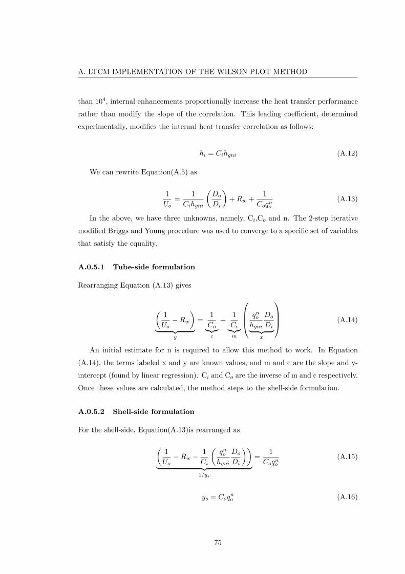
A. LTCM IMPLEMENTATION OF THE WILSON PLOT METHOD
than 104, internal enhancements proportionally increase the heat transfer performance
rather than modify the slope of the correlation. This leading coefficient, determined
experimentally, modifies the internal heat transfer correlation as follows:
hi = Cihgni (A.12)
We can rewrite Equation(A.5) as
1
Uo=
1
Cihgni
(Do
Di
)+Rw +
1
Coqno(A.13)
In the above, we have three unknowns, namely, Ci,Co and n. The 2-step iterative
modified Briggs and Young procedure was used to converge to a specific set of variables
that satisfy the equality.
A.0.5.1 Tube-side formulation
Rearranging Equation (A.13) gives
(1
Uo−Rw
)︸ ︷︷ ︸
y
=1
Co︸︷︷︸c
+1
Ci︸︷︷︸m
qnohgni
Do
Di︸ ︷︷ ︸x
(A.14)
An initial estimate for n is required to allow this method to work. In Equation
(A.14), the terms labeled x and y are known values, and m and c are the slope and y-
intercept (found by linear regression). Ci and Co are the inverse of m and c respectively.
Once these values are calculated, the method steps to the shell-side formulation.
A.0.5.2 Shell-side formulation
For the shell-side, Equation(A.13)is rearranged as
(1
Uo−Rw −
1
Ci
(qnohgni
Do
Di
))︸ ︷︷ ︸
1/ys
=1
Coqno(A.15)
ys = Coqno (A.16)
75
A. LTCM IMPLEMENTATION OF THE WILSON PLOT METHODAppendix A
ln |ys|︸ ︷︷ ︸y
= ln |Co|︸ ︷︷ ︸c
+ n︸︷︷︸m
ln |qo|︸ ︷︷ ︸x
(A.17)
In this step, the calculated values of Ci and Co are used to find the values of the
shell-side x and y. Once these are known, a linear regression may be performed to
find the values of m and c. Co is ec and n, the heat flux exponent in the pool boiling
correlation, is equal to m. Finally, a comparison may be made between the previous
step’s values of Co, Ci and n. The convergence criteria for the LTCM method requires
that all three vary by less than 0.01%. If this condition is not met, the values of the
variables are updated and the tube- and shell-side calculations are performed again.
A.0.5.3 Uncertainty propagation through the linear regression
In the previous section, it was mentioned that the slope and y-intercept of both the tube
and shell-side Wilson plots could be found through linear regression. This regression
could be as simple as utilizing a least-squares minimization algorithm. Such methods
have been utilized successfully and are well-documented (Liebenberg (2002)). However,
the least-squares linear regression method has several important drawbacks to consider.
Firstly, it is difficult to propagate the experimental uncertainty through the method,
and thus calculate the uncertainties in the variables. Second, the calculated values of x
and y have experimental uncertainties associated with them, which can be large, mainly
due to the uncertainty in the values of the heat flux measured. These are normally not
taken into account when performing a fit through the data. This means that the
accuracy of the fit might suffer due to a method trying to fit data that, because of their
large uncertainty, do not show the same trends as the great majority of the rest of the
data points. The method proposed by York et al. (2004) evaluates the least-squares
estimation at the least-squares adjusted points rather than at the observed points. In
their paper, the authors presented a method that unifies the standard errors when both
x and y data are subject to varying correlated errors. This method was adapted and
utilized to perform the linear regression in the modified LTCM method.
76
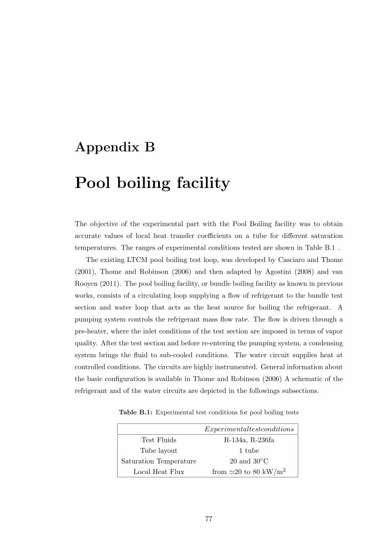
Appendix B
Pool boiling facility
The objective of the experimental part with the Pool Boiling facility was to obtain
accurate values of local heat transfer coefficients on a tube for different saturation
temperatures. The ranges of experimental conditions tested are shown in Table B.1 .
The existing LTCM pool boiling test loop, was developed by Casciaro and Thome
(2001), Thome and Robinson (2006) and then adapted by Agostini (2008) and van
Rooyen (2011). The pool boiling facility, or bundle boiling facility as known in previous
works, consists of a circulating loop supplying a flow of refrigerant to the bundle test
section and water loop that acts as the heat source for boiling the refrigerant. A
pumping system controls the refrigerant mass flow rate. The flow is driven through a
pre-heater, where the inlet conditions of the test section are imposed in terms of vapor
quality. After the test section and before re-entering the pumping system, a condensing
system brings the fluid to sub-cooled conditions. The water circuit supplies heat at
controlled conditions. The circuits are highly instrumented. General information about
the basic configuration is available in Thome and Robinson (2006) A schematic of the
refrigerant and of the water circuits are depicted in the followings subsections.
Table B.1: Experimental test conditions for pool boiling tests
Experimentaltestconditions
Test Fluids R-134a, R-236fa
Tube layout 1 tube
Saturation Temperature 20 and 30◦C
Local Heat Flux from '20 to 80 kW/m2
77
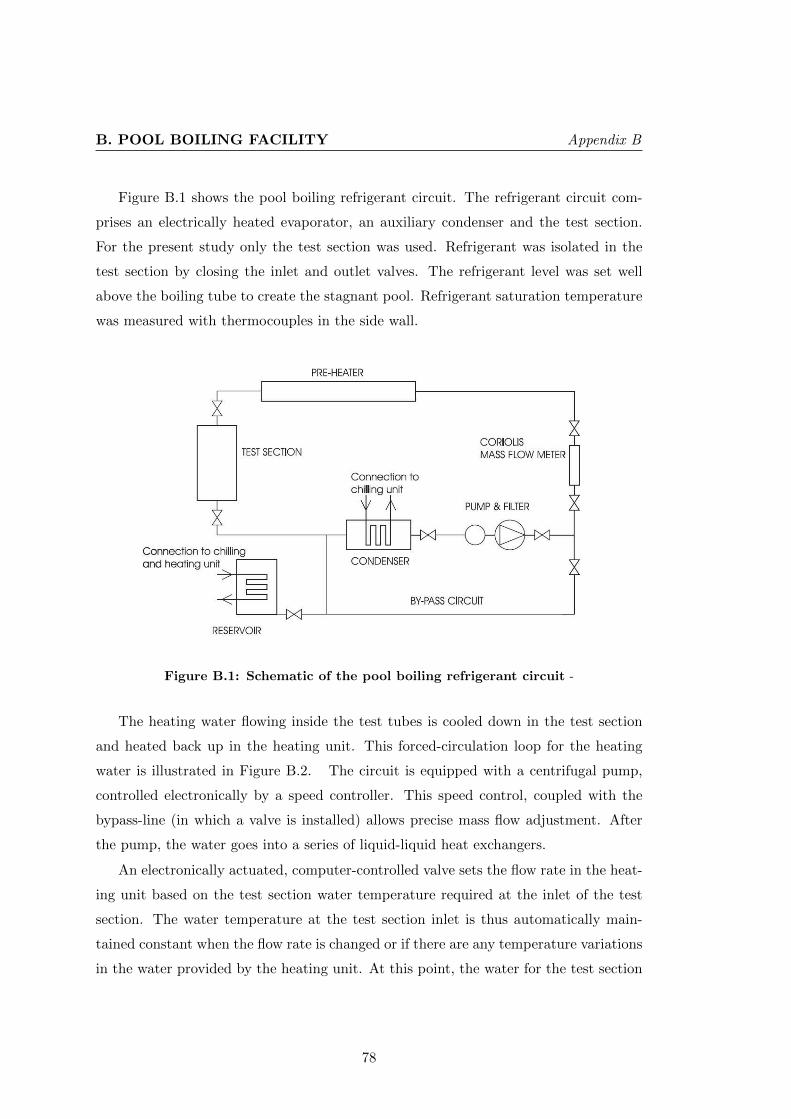
B. POOL BOILING FACILITY Appendix B
Figure B.1 shows the pool boiling refrigerant circuit. The refrigerant circuit com-
prises an electrically heated evaporator, an auxiliary condenser and the test section.
For the present study only the test section was used. Refrigerant was isolated in the
test section by closing the inlet and outlet valves. The refrigerant level was set well
above the boiling tube to create the stagnant pool. Refrigerant saturation temperature
was measured with thermocouples in the side wall.
Figure B.1: Schematic of the pool boiling refrigerant circuit -
The heating water flowing inside the test tubes is cooled down in the test section
and heated back up in the heating unit. This forced-circulation loop for the heating
water is illustrated in Figure B.2. The circuit is equipped with a centrifugal pump,
controlled electronically by a speed controller. This speed control, coupled with the
bypass-line (in which a valve is installed) allows precise mass flow adjustment. After
the pump, the water goes into a series of liquid-liquid heat exchangers.
An electronically actuated, computer-controlled valve sets the flow rate in the heat-
ing unit based on the test section water temperature required at the inlet of the test
section. The water temperature at the test section inlet is thus automatically main-
tained constant when the flow rate is changed or if there are any temperature variations
in the water provided by the heating unit. At this point, the water for the test section
78
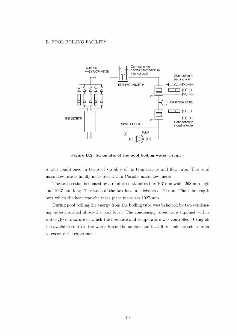
B. POOL BOILING FACILITY
Figure B.2: Schematic of the pool boiling water circuit -
is well conditioned in terms of stability of its temperature and flow rate. The total
mass flow rate is finally measured with a Coriolis mass flow meter.
The test section is housed by a reinforced stainless box 107 mm wide, 268 mm high
and 1067 mm long. The walls of the box have a thickness of 20 mm. The tube length
over which the heat transfer takes place measures 1027 mm.
During pool boiling the energy from the boiling tube was balanced by two condens-
ing tubes installed above the pool level. The condensing tubes were supplied with a
water-glycol mixture of which the flow rate and temperature was controlled. Using all
the available controls the water Reynolds number and heat flux could be set in order
to execute the experiment.
79

B. POOL BOILING FACILITY Appendix B
80
References
F. Agostini. Boiling on a Tube Bundle: Heat Transfer, Pressure Drop and Flow Pat-
terns. PhD thesis, Ecole Polytechnique Federale de Lausanne, Laboratory of Heat
and Mass Transfer, Lausanne, Switzerland, 2008. 21, 77
R. Armbruster and J. Mitrovic. Heat transfer in falling film on a horizontal tube. Heat
Transfer Conference - ASME, 12:13–21, 1995. 8
A. E. Bergles. Heat transfer augmentation. Two-Phase Flow Heat Exchangers, pages
343–373, 1988. 7
D. E. Briggs and E. H. Young. Modified Wilson plot techniques for obtaining heat
transfer correlation for shell and tube heat exchangers. Journal of Heat Transfer, 5:
51–56, 1969. 73, 74
S Casciaro and JR Thome. Thermal Performance of Flooded Evaporators, Part 2:
Review of Void Fraction, Two-Phase Pressure Drop, and Flow Pattern Studies. In
ASHRAE Trans., volume Vol. 107, pages 919–930, 2001. 21, 77
L. H. Chien and C. H. Cheng. A predictive model of falling film evaporation with
bubble nucleation on horizontal tubes. HVAC Research, 12:69–87, 2006. 12
L. H. Chien and R. L. Webb. A parametric study of nucleate boiling on structured
surfaces, part II: Effect of pore diameter and pore pitch. Journal of Heat Transfer,
120:1049–1054, 1998a. 7, 10
L. H. Chien and R. L. Webb. Visualization of pool boiling on enhanced surfaces.
Experimental Thermal and Fluid Science, 16:332–341, 1998b. 7, 10
81
M. Christians. Heat Transfer and Visualization of fallinf Film Evaporation on a Tube
Bundle. PhD thesis, Ecole Polytechnique Federale de Lausanne, Laboratory of Heat
and Mass Transfer, Lausanne, Switzerland, 2010. ii, 3, 11, 14, 15, 16, 17, 19, 21, 23,
24, 27, 30, 31, 32, 39, 40, 43, 44, 47, 57, 58, 61, 69, 74
S. W. Churchill and H. H. S. Chu. Correlating equations for laminar and turbulent free
convection from a vertical plate. International Journal of Heat and Mass Transfer,
18:1323–1329, 1975. 12, 13
M. C. Chyu and A. E. Bergles. Falling film evaporation on a horizontal tube. Multiphase
Flow and Heat Transfer, ASME HTD, 43:39–48, 1985. 6
M. C. Chyu and A. E. Bergles. An analytical and experimental study of falling-film
evaporation on a horizontal tube. Journal of Heat Transfer, 109:983–990, 1987. 8,
12
M. G. Cooper. Heat flow rates in saturated nucleate pool boiling - a wide-ranging
examination using reduced properties. Advances in Heat Transfer, 16:157–239, 1984.
62, 74
L. S. Fletcher, V. Sernas, and L. Galowin. Evaporation from thin water films on
horizontal tubes. Ind. Eng. Chem., Process Des. Dev., 13:265–269, 1974. 8, 9
L. S. Fletcher, V. Sernas, and W. H. Parken. Evaporation heat transfer coefficients for
thin sea water films on horizontal tubes. Ind. Eng. Chem., Process Des. Dev., 14:
411–416, 1975. 8
Y. Fujita and M. Tsutsui. Evaporation heat transfer of falling films on horizontal tubes.
Part 2: Experimental study. Heat Transfer - Japanese Research, 24:17–31, 1995. 9,
12
Y. Fujita and M. Tsutsui. Experimental investigation of falling film evaporation on
horizontal tubes. Heat Transfer - Japanese Research, 27:609–618, 1998. 5
E. N. Ganic and D. Getachew. Effects of surface condition and working fluid on liquid
film breakdown during heat transfer. In 8th International Heat Transfer Conference,
pages 1931–1936, 1986. 4
82
E. N. Ganic and M. N. Roppo. An experimental study of falling liquid film breakdown
on a horizontal cylinder during heat transfer. Journal of Heat Transfer, 102:342–346,
1980. 8
V. Gnielinski. New equations for heat and mass transfer in turbulent flow through
pipes and ducts. Forschung Im. Ingenieurwessen, 41(1):1975, 1975. 12, 37, 74
U. Gross. Falling film evaporation in a closed thermosyphon. In International Heat
Transfer Conference, Brighton, England, volume 7, pages 443–448, 1994. 4
D. Gstohl. Heat Transfer and Flow Visualization of Falling Film Condensation on Tube
Arrays with Plain and Enhanced Surfaces. PhD thesis, Ecole Polytechnique Federale
de Lausanne, Laboratory of Heat and Mass Transfer, Lausanne, Switzerland, 2004.
21, 23, 74
D. Gstohl and J. R. Thome. Visualization of R-134a Flowing on Tube Arrays with
Plain and Enhanced Surfaces under Adiabatic and Condensing Conditions. Heat
Transfer Engineering, 27, 2006. 3
M. Habert. Falling Film Evaporation on a Tube Bundle with Plain and Enhanced Tubes.
PhD thesis, Ecole Polytechnique Federale de Lausanne, Laboratory of Heat and Mass
Transfer, Lausanne, Switzerland, 2009. 11, 13, 14, 16, 18, 19, 21, 23, 39
M. Habert, G. Ribatski, and J. R. Thome. Experimental study on falling film flow
pattern map and intercolumn distance with R-236fa. 2006. 3
H. Honda, S. Nozu, and Y. Takeda. Flow characteristics of condensate on a vertical
column of horizontal low finned tubes. In Proc. ASME-JSME Thermal Engineering
Joint Conference, Honolulu, volume 1, pages 517–524, 1987. 3
X. Hu and A. M. Jacobi. The intertube falling film, part 1: Flow characteristics, mode
transitions, and hysteresis. Journal of Heat Transfer, 118:616–625, 1996. 9
H. F. Khartabil, R. N. Christensen, and D. E. Richards. A modified Wilson-plot
technique for determining heat transfer correlations. Proceedings of the Second UK
National Conference on Heat Transfer, 11:1331–1357, 1988. 73
83
S. J. Kline and F. A. McClintock. Describing uncertainties in single-sample experiments.
Mechanical Engineering, 75:3–8, 1953. 56
S. S. Kutateladze. On the transition to film boiling under natural convection. Kotlo-
turbostroenie, 3:152–158, 1948. 20
L. Liebenberg. A Unified Prediction Method for Smooth and Microfin Tube Condensa-
tion Performance. PhD thesis, Rand Afrikaans University, Department of Mechanical
Engineering, 2002. 76
J. J. Lorenz and D. Yung. A note to combined boiling and evaporation of liquid films
on horizontal tubes. Transactions of the ASME, 101:178–180, 1979. 12
J. Mitrovic. Flow structures of a liquid film falling on horizontal tubes. Chemical
Engineering & Technology, 28(6):684 – 694, 2005. 3
S. A. Moeykens and M. B. Pate. Spray evaporation heat transfer of R-134a on plain
tubes. ASHRAE Transactions, 100:173–184, 1994. 8, 9
S. A. Moeykens, W. W. Huebsch, and M. B. Pate. Heat transfer of R-134a in single tube
spray evaporation including lubrificant effect and enhanced surface results. ASHRAE
Transactions, 101(1):111–123, 1995a. 8, 10
S. A. Moeykens, B. J. Newton, and M. B. Pate. Effects of surface enhancement, film
feed-supply rate, and bundle geometry on spray evaporation heat transfer perfor-
mance. ASHRAE Transactions, 101(2):408–419, 1995b. 8
National Institute of Standards and Technology. NIST Thermodynamic Properties of
Refrigerants and Refrigerant Mixtures Database. ver 8.0, Gaithersburg, MD, 2002.
33
J. A. Olivier. Single-phase heat transfer and pressure drop inside Horizontal Circular
Smooth and Enhanced Tubes with different inlet configurations for transitional flow.
PhD thesis, University of Pretoria, Department of Mechanical and Aeronautical En-
gineering, 2008. 74
W. H. Parken and L. S. Fletcher. Heat transfer in liquid thin films flowing over hor-
izontal tubes. In Proceedings of the 7th International Heat Transfer Conference,
volume 4, pages 415–420, 1982. 8
84
W. H. Parken, L. S. Fletcher, V. Sernas, and J. C. Han. Heat transfer through falling
film evaporation and boiling on horizontal tubes. Transactions of ASME, 112:744–
750, 1990. 8
B. S. Petukhov. Heat transfer and friction in turbulent pipe flow with variable physical
properties. Advances in Heat Transfer, 6:503–564, 1970. 74
M.E. Poniewski and J. R. Thome. Nucleate Boiling on Micro-structured Surfaces.
www.htri-net.com/ePubs/epubs.htm, 2008. 7
G. Ribatski and A. M. Jacobi. Falling-film evaporation on horizontal tubes – a critical
review. International Journal of Refrigeration, 28:635–653, 2005. 4, 8
G. Ribatski and J. R. Thome. Experimental study on the onset of local dryout in an
evaporating falling film on horizontal plain tubes. Experimental Thermal and Fluid
Science, 31:483–493, 2007. 12, 13, 16, 17, 19
W. M. Rohsenow, J. P. Hartnett, and E. N. Ganic. Handbook of heat transfer funda-
mentals – Chapter 12 – Thin-Film Heat Transfer. New York : McGraw-Hill, 1985.
6
J. F. Roques. Falling Film Evaporation on a single tube and on a tube bundle. PhD
thesis, Ecole Polytechnique Federale de Lausanne, Laboratory of Heat and Mass
Transfer, Lausanne, Switzerland, 2004. 8, 11, 19, 21, 23, 39, 74
J. F. Roques and J. R. Thome. Falling film transitions between droplet, column, and
sheet flow modes on a vertical array of horizontal 19 fpi and 40 fpi low-finned tubes.
Heat Transfer Engineering, 24(6):40–45, 2003. 3
J. F. Roques and J. R. Thome. Falling films on arrays of horizontal tubes with R-
134a, part I: Boiling heat transfer results for four types of tubes. Heat Transfer
Engineering, 28(5):398–414, 2007a. 10, 13, 14, 16, 17
J. F. Roques and J. R. Thome. Falling films on arrays of horizontal tubes with R-
134a, part II: Flow visualization, onset of dryout, and heat transfer predictions. Heat
Transfer Engineering, 28(5):415–434, 2007b. 11
85
J. F. Roques, V. Dupont, and J. R. Thome. Falling film transitions on plain and
enhanced tubes. Journal of Heat Transfer, 124(3):491–499, 2002. 3
J. W. Rose. Heat-transfer coefficients, wilson plots and accuracy of thermal measure-
ments. Experimental Thermal and Fluid Science, 28(2-3):77–86, 2004. 73
Teresa B. Styrylska and Agnieszka A. Lechowska. Unified wilson plot method for
determining heat transfer correlations for heat exchangers. Journal of Heat Transfer,
125(4):752–756, 2003. 73
J. R. Thome. Enhanced Boiling Heat Transfer. Hemisphere Publishing Corporation,
1990. 7
J. R. Thome. Engineering Databook III. Wolverine www.wlv.com, 2006. 3, 5
J.R. Thome and D.M. Robinson. Prediction of Local Bundle Boiling Heat Transfer
Coefficients: Pure Refrigerant Boiling on Plain, Low Fin and Turbo-BII HP Tube
Bundles. Heat Transfer Engineering, 2006. doi: NA. 21, 77
E. van Rooyen. Frequency analysis of boiling flow on a bundle of tubes. PhD thesis,
Ecole Polytechnique Federale de Lausanne, Laboratory of Heat and Mass Transfer,
Lausanne, Switzerland, 2011. 21, 62, 66, 70, 77
E. E. Wilson. A basis for rational design of heat transfer apparatus. ASME transactions,
37:546–668, 1915. 72, 73
Derek York, Norman M. Evensen, Margarita Lopez Martinez, and Jonas De Basabe
Delgado. Unified equations for the slope, intercept, and standard errors of the best
straight line. American Journal of Physics, 72(3):367–375, 2004. 76
X. Zeng, M. C. Chyu, and Z. H. Ayub. Evaporation heat transfer performance of
nozzle-sprayed ammonia on a horizontal tube. ASHRAE Transactions, 101:136–149,
1996. 8, 9
86