satin: a R package for extracting and visualizing satellite data for oceanographic applications

Héctor VILLALOBOS1 and Eduardo GONZÁLEZ-RODRÍGUEZ2

1 Centro Interdisciplinario de Ciencias MarinasInstituto Politécnico Nacional (CICIMAR-IPN)

(supported by COFAA)

2 Centro de Investigación Científica y de Educación Superior de Ensenada (CICESE), Unidad La Paz

La Paz, Baja California Sur, MEXICO

The R User Conference 2009July 8-10, Agrocampus-Ouest, Rennes, France

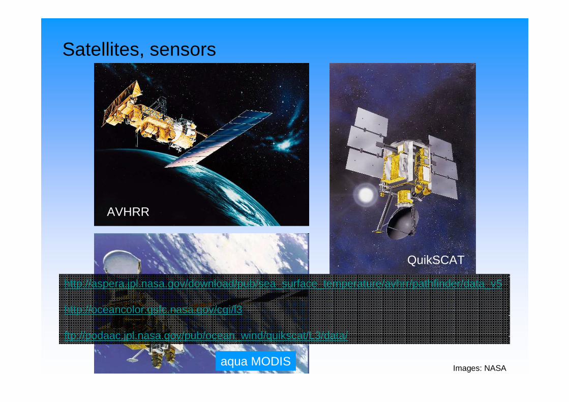
aqua MODIS

AVHRR

Satellites, sensors

QuikSCAT

Images: NASA

http://aspera.jpl.nasa.gov/download/pub/sea_surface_temperature/avhrr/pathfinder/data_v5

http://oceancolor.gsfc.nasa.gov/cgi/l3

ftp://podaac.jpl.nasa.gov/pub/ocean_wind/quikscat/L3/data/

Hierarchical Data Format (hdf) files

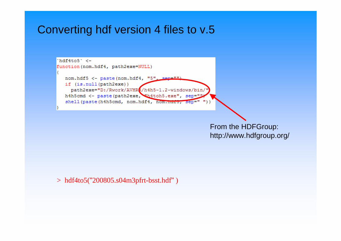
Converting hdf version 4 files to v.5

> hdf4to5("200805.s04m3pfrt-bsst.hdf" )

From the HDFGroup:http://www.hdfgroup.org/

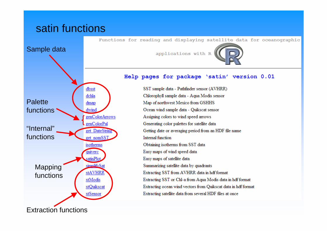
satin functions

Sample data

Extraction functions

Mappingfunctions

“Internal”functions

Palettefunctions

[1] "2007"[1] "Jan 2000"[1] "1 - 8 Jan 2000"[1] "1 - 5 Jan 2000"[1] "5 Jan 2007"[1] "31 Jan - 4 Feb 2009"[1] "1 - 31 Jul 2007"[1] "1 - 31 May 2008"[1] "31 Dec 2008"[1] "Week 1 2009"

> fnames <- c("2007.s04y3pfrt-bsst.hdf","200001.s04m3pfv50-bsst-16b.hdf", "2000001-2000008.s0483pfv50-bsst-16b.hdf", "2000001-2000005.s0453pfv50-bsst-16b.hdf", "2007005.s04d3pfrt-bsst.hdf", "2009031-2009035.s0453pfrt-sst.hdf", "A20071822007212.L3m_MO_SST_4.hdf5", "A20081222008152.L3m_MO_CHLO_4.hdf5", "QS_XWGRD3_2008366.20090021524.hdf5", "200901.s04w3pfrt-bsst.hdf“)

> for (i in 1:length(fnames)) { + av.perio <- get_DateString( fnames[i] )+ print(av.perio) + }

Internal functions

get_DateString( )get_nomSST( )

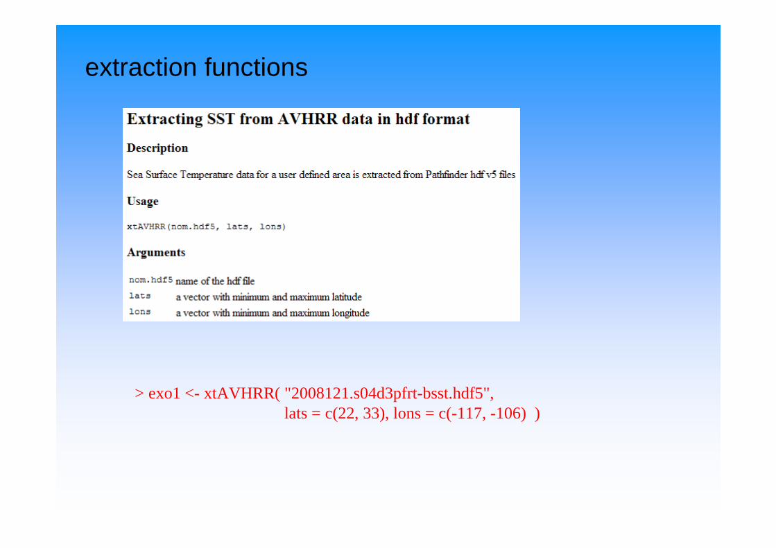
extraction functions

> exo1 <- xtAVHRR( "2008121.s04d3pfrt-bsst.hdf5", lats = c(22, 33), lons = c(-117, -106) )

> class(exo1)[1] "list"

Structure of returned object

> names(exo1)[1] "longitude" "latitude" "sst" "period"

> exo1$longitude[1:5][1] -116.96 -116.91 -116.87 -116.83 -116.78

> exo1$latitude[1:5][1] 22.03 22.08 22.12 22.17 22.21

> exo1$sst[1:5, 1:5][,1] [,2] [,3] [,4] [,5]

[1,] 20.175 20.175 20.175 20.250 20.250[2,] 20.175 20.175 20.175 20.175 20.175[3,] 20.025 20.100 20.100 20.100 20.100[4,] 20.025 20.025 20.025 20.025 20.100[5,] 20.025 20.025 20.025 20.025 20.025

> exo1$period[1] "30 Apr 2008"

extraction functions

exo2 <- xtModis("A20081212008128.L3m_8D_CHLO_4.hdf5", lats = c(22, 33), lons = c(-117, -106) )

And also the structure of the returned object

Idem for QuikSCAT:exo3 <- xtQuikscat("QS_XWGRD3_2008121.20081230017.hdf5",

lats=c(22, 33), lons=c(-117, -106) )

But its structure differs a little:

> class(exo2)[1] "list“

> names(exo2)[1] "longitude" "latitude" “param" "period"

The extraction for aqua Modis is the same

> names(exo3)[1] "longitude" "latitude" "ucomp" "vcomp" "period"

mapping functions (SST, Sea Surface Temperature, °C)

> satinPlot(exo1)

satinPlot(xyz, xlims = NULL, ylims = NULL, zlims = NULL, map = NULL,map.col = "grey", map.outline = "black", colimg = NULL, xlab = "longitude", ylab = "latitude", colbar = TRUE, colbar.pos = "r", xoffs = 0, yoffs = 0, main = NULL, main.pos = "tr", ...)

Map was obtained from:

“Global Self-consistent Hierarchical High-resolution Shoreline Database”(GSHHS)

with function:

Rgshhs(maptools)

> satinPlot(exo1, map = nwmexico, map.col = "grey50", map.outline = "black", yoffs =1.2)

mapping functions (SST, Sea Surface Temperature, °C)

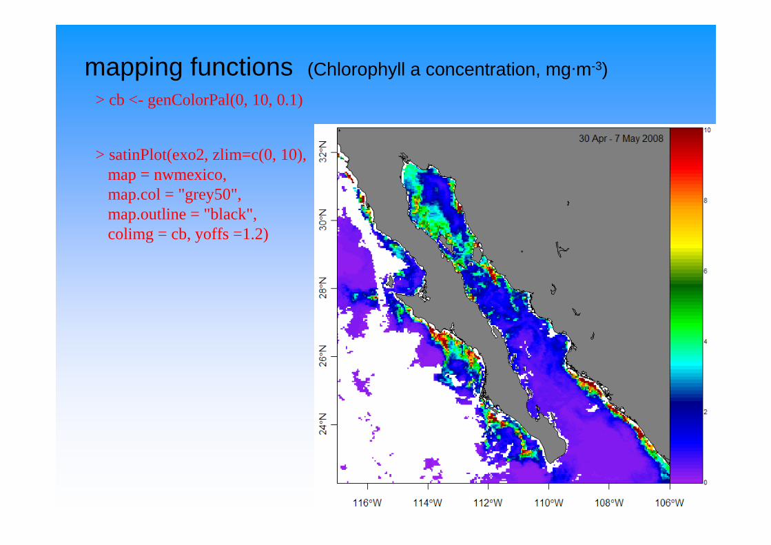
> cb <- genColorPal(0, 10, 0.1)

> satinPlot(exo2, zlim=c(0, 10), map = nwmexico, map.col = "grey50", map.outline = "black", colimg = cb, yoffs =1.2)

mapping functions (Chlorophyll a concentration, mg·m-3)

> quiverc(exo3, pass="mean")

quiverc(qso, pass, scale=1, length=0.05, colarrow=NULL, add2map=FALSE, ra.pos=NULL, ra.speed=NULL, ra.col="black", map=NULL,map.col="grey", map.outline="black", colbar=FALSE, colbar.pos="r",main=NULL, main.pos="tr", ...)

mapping functions (Ocean wind speed, m·s-1)

> cb2 <- genColorPal(0, 11, 1)> cb2$pal[1] "#A020F0" "#0F03FD" "#0000A2" "#00B2DC" "#00FF65"[6] "#00B100" "#65A100" "#FFE400" "#FF8300" "#F30000"[11] "#8B0000"

$breaks[1] 0 1 2 3 4 5 6 7 8 9 10 11

> quiverc(exo3, pass = "mean", scale = 0.7, colarrow = colarr,add2map = FALSE, ra.pos =c(-108, 30), ra.speed = 10,ra.col = "red", map = nwmexico,map.col = "grey", map.outline ="black", colbar = TRUE,colbar.pos = "r")

> colarr <- genColorArrows(exo3, pass="mean", cb2)

mapping functions (Ocean wind speed, m·s-1)

> satinPlot(exo2, zlim=c(0, 20), map = nwmexico, map.col = "grey50", …)

> quiverc(exo3, pass="mean", scale=0.7, colarrow="grey80", add2map=TRUE, ra.pos=c(-108, 32),ra.speed=10, main="")

mapping functions (overlaying wind vectors)

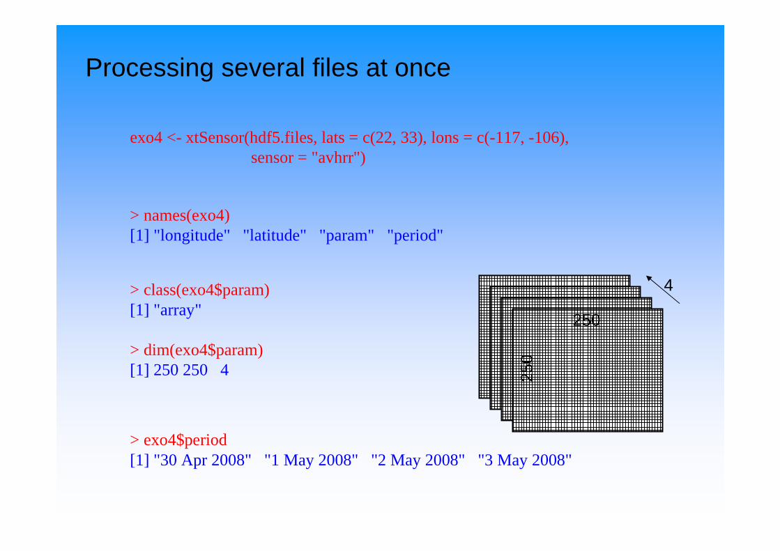
Processing several files at once

exo4 <- xtSensor(hdf5.files, lats = c(22, 33), lons = c(-117, -106), sensor = "avhrr")

> names(exo4)[1] "longitude" "latitude" "param" "period"

> class(exo4$param)[1] "array"

> dim(exo4$param)[1] 250 250 4

> exo4$period[1] "30 Apr 2008" "1 May 2008" "2 May 2008" "3 May 2008"

250

250

4

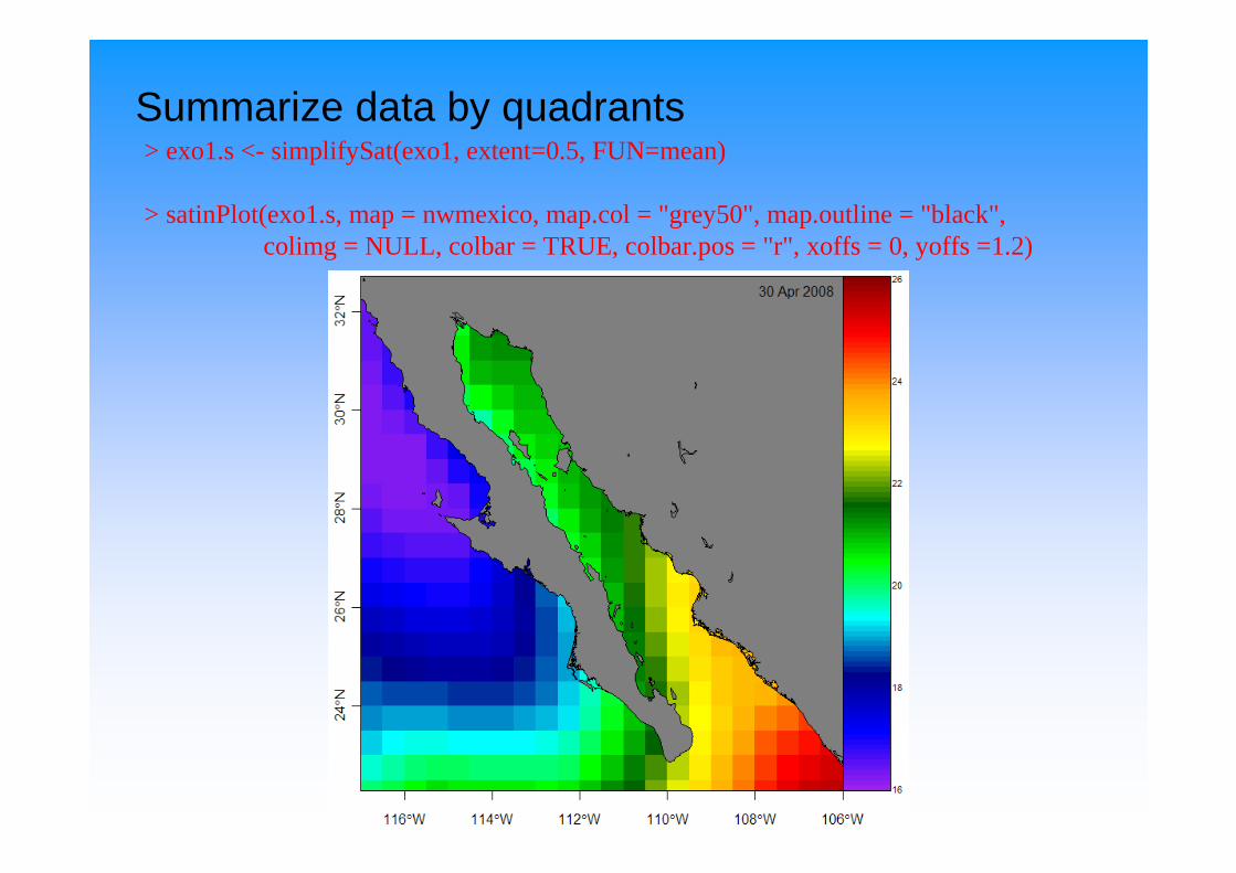
Summarize data by quadrants > exo1.s <- simplifySat(exo1, extent=0.5, FUN=mean)

> satinPlot(exo1.s, map = nwmexico, map.col = "grey50", map.outline = "black", colimg = NULL, colbar = TRUE, colbar.pos = "r", xoffs = 0, yoffs =1.2)

Obtaining isotherms> isot <- isotherms(exo1, tlevels=c(19, 21))

> satinPlot(exo1, map = nwmexico, map.col = "grey50“)> addLines(isot$PolySet, col="grey90", lwd=2, lty=c(1, 2) )

References

David James and Kurt Hornik (2009). chron: Chronological Objects which Can Handle Dates andTimes. R package version 2.3-30.

Original S code by Richard A. Becker and Allan R. Wilks. R version by Ray Brownrigg Enhancementsby Thomas P Minka <surname@stat.cmu.edu> (2009). maps: Draw Geographical Maps. R package version 2.1-0. http://CRAN.R-project.org/package=maps

Nicholas J. Lewin-Koh and Roger Bivand, contributions by Edzer J. Pebesma, Eric Archer, AdrianBaddeley, Hans-Jörg Bibiko, Stéphane Dray, David Forrest, Patrick Giraudoux, Duncan Golicher,Virgilio Gómez Rubio, Patrick Hausmann, Thomas Jagger, Sebastian P. Luque, Don MacQueen,Andrew Niccolai and Tom Short (2009). maptools: Tools for reading and handling spatial objects. R package version 0.7-23. http://CRAN.R-project.org/package=maptools

Jon T. Schnute, Nicholas Boers, Rowan Haigh and Alex Couture-Beil. (2008). PBSmapping: PBS Mapping 2.59. R package version 2.59.

Marcus G. Daniels mdaniels@lanl.gov (). hdf5: HDF5. R package version 1.6.9.

Jim Lemon, Ben Bolker, Sander Oom, Eduardo Klein, Barry Rowlingson, Hadley Wickham, Anupam Tyagi, Olivier Eterradossi, Gabor Grothendieck, Michael Toews, John Kane, Mike Cheetham, Rolf Turner, Carl Witthoft, Julian Stander, Thomas Petzoldt, Remko Duursma,Elisa Biancotto and Ofir Levy (2009). plotrix: Various plotting functions. R package version 2.6. http://CRAN.R-project.org/package=plotrix

Thank you!http://www.cicimar.ipn.mx

http://www.cicese.mx