MNRAS 000, 1–15 (2018) Preprint 24 August 2018 Compiled using MNRAS LATEX style file v3.0

Satellites Form Fast & Late: a Population Synthesis for theGalilean Moons

M. Cilibrasi1,2,3?, J. Szulagyi3,4, L. Mayer3, J. Drazkowska3,5, Y. Miguel6,7, P. Inderbitzi31Scuola Normale Superiore, Piazza dei Cavalieri 7, I-56126 Pisa, Italy2Dipartimento di Fisica ”Enrico Fermi”, Universita di Pisa, Largo Pontecorvo 3, I-56127 Pisa, Italy3Centre for Theoretical Astrophysics and Cosmology, Institute for Computational Science, University of Zurich,Winterthurerstrasse 190, CH-8057 Zurich, Switzerland4ETH Zurich, Institute for Particle Physics and Astrophysics, Wolfgang-Pauli-Strasse 27, CH-8093, Zurich, Switzerland5University Observatory, Faculty of Physics, Ludwig-Maximilians-Universitat Munchen, Scheinerstr. 1, 81679 Munich, Germany6Observatoire de la Cote d’Azur, Boulevard de l’Observatoire, CS 34229 F-06304, Nice Cedex 4, France7Leiden Observatory, University of Leiden, Niels Bohrweg 2, NL-2333CA Leiden, The Netherlands

Accepted 2018 August 6. Received 2018 August 6; in original form 2018 January 10

ABSTRACTThe satellites of Jupiter are thought to form in a circumplanetary disc. Here we addresstheir formation and orbital evolution with a population synthesis approach, by varyingthe dust-to-gas ratio, the disc dispersal timescale and the dust refilling timescale. Thecircumplanetary disc initial conditions (density and temperature) are directly drawnfrom the results of 3D radiative hydrodynamical simulations. The disc evolution istaken into account within the population synthesis. The satellitesimals were assumedto grow via streaming instability. We find that the moons form fast, often within 104

years, due to the short orbital timescales in the circumplanetary disc. They form insequence, and many are lost into the planet due to fast type I migration, pollutingJupiter’s envelope with typically 15 Earth-masses of metals. The last generation ofmoons can form very late in the evolution of the giant planet, when the disc hasalready lost more than the 99% of its mass. The late circumplanetary disc is coldenough to sustain water ice, hence not surprisingly the 85% of the moon populationhas icy composition. The distribution of the satellite-masses is peaking slightly aboveGalilean masses, up until a few Earth-masses, in a regime which is observable with thecurrent instrumentation around Jupiter-analog exoplanets orbiting sufficiently closeto their host stars. We also find that systems with Galilean-like masses occur in 20%of the cases and they are more likely when discs have long dispersion timescales andhigh dust-to-gas ratios.

Key words: planets and satellites, formation - planets and satellites, gaseous planets- planets and satellites, general

1 INTRODUCTION

In the last few years theories about our Solar System forma-tion took a step forward thanks to a more precise compre-hension of giant planet formation and evolution within pro-toplanetary discs. Today the two main models in this fieldare the Gravitational Instability scenario, or GI (Boss 1997;Durisen et al. 2007), when a self-gravitating gaseous clumpdirectly collapses into a giant planet, and the Core Accretionmodel, or CA (Pollack et al. 1996), that occurs when colli-sions and coagulation of dust particles form a solid planetary

? E-mail: marco.cilibrasi@alumni.sns.it

embryo, massive enough to accrete and maintain a gaseousenvelope. Both of these theories predict the presence of cir-cumplanetary discs (CPDs) made of gas and dust rotatingaround the forming planet in the last stage of formation (Al-ibert et al. 2005; Ayliffe & Bate 2009; Ward & Canup 2010;Szulagyi et al. 2017a,b). Even though these discs are similarto protoplanetary discs (PPDs) around young stars, thereare significant differences among them. The most importantone is that the CPDs are continuously fed by a vertical in-flux of gas and well coupled dust from the protoplanetarydisc upper layers, due to gas accretion onto the central giantplanet (Tanigawa et al. 2012; Szulagyi et al. 2014).

Due to the fact that regular satellites (including themoons of Jupiter) are commonly thought to form in CPDs,

© 2018 The Authors

arX

iv:1

801.

0609

4v3

[as

tro-

ph.E

P] 2

3 A

ug 2

018

2 Cilibrasi et al.

the understanding of the properties of these discs is cru-cial to address satellite formation. With no observationalconstraints about them, so far we have to rely on hydrody-namic simulations to study the initial CPD that have formedthe Galilean satellites (e.g. Ayliffe & Bate 2009; Gressel etal. 2013; Szulagyi et al. 2017b). The properties of Jupiter’sfour biggest moons, however, provide some constraints aboutthe features of this disc. Voyager and Galileo missions re-vealed that Io is rocky, while the outer three moons con-tain significant amount of water ice (Showman & Malhotra1999). The accretion of icy satelletesimals is only possiblein a CPD which has a bulk temperature below the waterfreezing point, ∼180 K. However, hydrodynamic simulationsof CPDs found the temperature to be significantly higherthan that, often peaking at several thousands of Kelvins(e.g. Ayliffe & Bate 2009; Szulagyi et al. 2016). The studyof Szulagyi (2017) showed that even accounting for the cool-ing of the planet (due to radiating away its formation heat),the Jupiter surface temperature had to be significantly lowerthan 1000 K, when the Galilean satellites have formed, oth-erwise the CPD cannot form icy satellites. This indicatedthat the moons had to form very late in the planet- & disc-evolution, when Jupiter has significantly cooled off and itsCPD was dissipating (moving towards the optically thin,and hence cold regime).

Regarding the mass of the CPD, we know that thetotal mass of the Galilean satellites is ∼ 2 × 10−4Mplanet(Mp hereafter), same as in the case of Saturn (Canup &Ward 2006). Because this value considers only solids, witha standard dust-to-gas ratio of 0.01 one gets a CPD mass of∼ 2 × 10−2Mp. However, as the Canup & Ward works havepointed out (Canup & Ward 2002, 2006, 2009), this is theintegrated CPD mass, i.e. at a snapshot of time the CPD canbe much lighter than this while still producing Galilean masssatellites over the years (gas-starved disc model). Due to thecontinuous feeding from the protoplanetary disc, throughoutthe lifetime of the CPD, even orders of magnitude more ma-terial could have been processed through the CPD. The massof the disc has been certainly enough to make several gen-erations of Galilean-mass moons, and several of them couldhave been lost into the planet through migration, openingthe idea of sequential satellite-formation (Canup & Ward2002).

There have been several different approaches to studysatellite formation, starting from works that studied condi-tions of the CPD during satellite formation and constraintson this disc based on the properties of the Galilean moons(Canup & Ward 2009, 2002; Estrada et al. 2009). Recently,Fujii et al. (2017) numerically solved a 1D-model of cir-cumplanetary disc long term evolution and the migrationof satellites in it. They found that the moonlets are oftencaptured in resonances, which could explain the formationof the first three resonant satellites. A population synthe-sis work made by Sasaki et al. (2010) modeled the initialcircumplanetary disc density profile solving a 1D equationfor its viscous evolution (Pringle 1981) with an inner cavitybetween the planet and disc. They included satellite accre-tion with gravitational focusing and the type I migrationtimescale using the formula from Tanaka et al. 2002. Build-ing a semi-analytical model and performing a populationsynthesis varying the location of the initial seeds, the α vis-cosity and the dispersion time of the disc, they found that

in 70% of their runs they had 4 or 5 satellites, often lockedin a resonant configuration thanks to the inner cavity of thedisc. They varied the initial circumplanetary disc profilesand used quite different models than what recent hydro-dynamic models on the CPD predict (e.g. Ayliffe & Bate2009, Tanigawa et al. 2012, Szulagyi et al. 2014, Szulagyi2017). Same is true for the Miguel & Ida (2016), which usedthe Minimum Mass SubNebula (MMSN) as an initial CPDprofile (Mosqueira & Estrada 2003). They studied the evo-lution of about 20 satellite-seeds, with initial positions ran-domly chosen in the disc, together with the gas density of thedisc (but without the temperature evolution in their case),considering also the dust depletion caused by the accretionof dust itself onto protosatellites. Different runs have beenmade with different disc parameters, such as the dust-to-gas ratio of the disc, its dispersion timescale and the initialmass of satellitesimals, using then a population synthesisapproach to analyse the outcomes.

Other different approaches to satellite formation aroundgas giants are, for instances in Heller & Pudritz (2015a,b)and in Moraes et al. (2017). In the first two works the au-thors built a semi-analytical model for the CPD structureand evolution, considering different heating processes (vis-cous heating, accretion onto the CPD, radiation from the hotplanet, and radiation from the star) in order to study howthe ice line changes position over time during the evolutionof the whole system. They found that in order to reproducethe actual compositions of the Galilean satellites, the moonsthemselves have to form late in Jupiter evolution, when thedisc is sufficiently cold, that agrees with the sequential for-mation process. In the latter case the authors performedN-body simulations with satellitesimals in a minimum masssubnebula circumplanetary disc, considering various eccen-tricities and inclinations of their orbits. In their simulationsthey found that satellites should never open a gap in theCPD because they are not massive enough and that initialeccentricities and inclinations do not affect results becauseof the gas damping.

Because previous works have used CPD profiles thatwere derived from the current composition and location ofthe Galilean satellites without taking into account their mi-gration and the possibility for several lost satellites system,here we present a population synthesis (Benz et al. 2014)on CPD profiles that are consistent with recent radiativehydrodynamical simulations on the circum-Jovian disc. Wealso take into account the thermal evolution of the disc, andthe continuous feeding of gas and dust from the vertical in-flux from the protoplanetary disc (e.g. Tanigawa et al. 2012;Szulagyi et al. 2014; Fung & Chiang 2016). Moreover, we usea dust-coagulation and evolution code to calculate the initialdust density profile corresponding to the gas hydrodynamicsof Szulagyi (2017). We assumed that the initial seeds wereformed via streaming instability (e.g. Youdin & Goodman2005), and we placed these moonlets at the location wherethe conditions for streaming instability are satisfied (e.g. thelocal dust-to-gas ratio is higher than unity).

MNRAS 000, 1–15 (2018)

Formation of the Galilean Satellites 3

2 METHODS

2.1 Hydrodynamic simulation

For the circumplanetary disc density and temperature pro-files we used a simulation from Szulagyi (2017). Among thevarious models in that paper considering different planetarytemperatures, we used here one of the coldest (most evolved)state with planetary temperature of 2000 K. This is becausethe satellites of Jupiter are icy, they had to form in a cold cir-cumplanetary disc, when the planet has cooled off efficiently(Szulagyi 2017). This is only true in the very late stage ofcircumplanetary disc evolution, close to the time when thecircumstellar disc has dissipated away.

Our hydrodynamic simulation was performed with theJUPITER hydrodynamic code (de Val-Borro et al. 2006;Szulagyi et al. 2016) developed by F. Masset & J. Szulagyi.This code is three dimensional, grid-based, uses the finite-volume method and solves the Euler equations, the totalenergy equation and the radiative transfer with flux limiteddiffusion approximation, according to the two-temperatureapproach (e.g. Kley 1989; Commercon et al. 2011). The sim-ulation contained a circumstellar disc between 2.08 AU till12.40 AU (sampled in 215 cells radially), with an initialopening angle of 7.4 degrees (from the midplane to the discsurface, using 20 cells). The coordinate system in the sim-ulation was spherical, centreed on the Sun-like star and co-rotating with the planet. The initial surface density was apower-law function with 2222kgm−2 at the planet’s locationat 5.2 AU and an exponent of -0.5. The planet was a Jupiteranalog, which reached its final mass through 30 orbits. Thecircumstellar disc azimuthally ranged over 2π sampled into680 cells. To have sufficient resolution on the circumplane-tary disc developed around the gas-giant, we placed 6 nestedmeshes around the planet, each doubling the resolution ineach spatial direction. Therefore, on the highest resolutionmesh the sampling was ∼ 80% of Jupiter-diameter (∼ 112000km) for a cell-diagonal. For the boundaries and resolution ofeach refined level, we used the same as Table 1 in Szulagyiet al. (2016). Because the resolution is sub-planet resolution,at the planet location we fixed the temperature to 2000 K(thereafter referred as planet temperature) within 3 RJupiter,corresponding an evolved, late stage of the circumstellar discand planet system, roughly around 1-2 Myrs (Mordasini etal. 2017).

The equation of state in the simulation was ideal gas –P = (γ−1)Eint – which connects the internal energy (Eint) withthe pressure (P) through the adiabatic exponent: γ = 1.43.For the viscosity, we solve the viscous stress tensor to set aconstant, kinematic (physical) viscosity, that equals to 0.004α-viscosity at the planet location. Due to the radiative mod-ule and the energy equation, the gas can heat up throughviscous heating, adiabatic compression and cool through ra-diation and adiabatic expansion. The opacity table used inthe code was of Bell & Lin (1994) that contains both the gasand dust Rosseland-mean opacities. Therefore, even thoughthere is no dust component explicitly included into the sim-ulations, the dust contribution to the temperature is takeninto account through the dust-to-gas ratio, that was cho-sen to be 0.01, i.e. equal to the interstellar medium value(Boulanger et al. 2000). The mean-molecular weight was setto 2.3, which corresponds to solar composition. The rest of

the parameters and process of the simulation can be foundin Szulagyi (2017) and Szulagyi et al. (2016).

2.2 Population synthesis

Our semi-analytical model essentially consists of a circum-planetary disc in which protosatellites can migrate, accretemass and be lost into the central planet. In the meantime,while the disc density and temperature evolve in time, it cre-ates newer and newer protosatellites. The units in our pop-ulation synthesis are the following: Rp as planet radius, Mp

(planetary mass), time in years and temperature in Kelvin.When referring to the specific case of Jupiter, MJ is used asthe unit for masses.

2.2.1 Disc structure

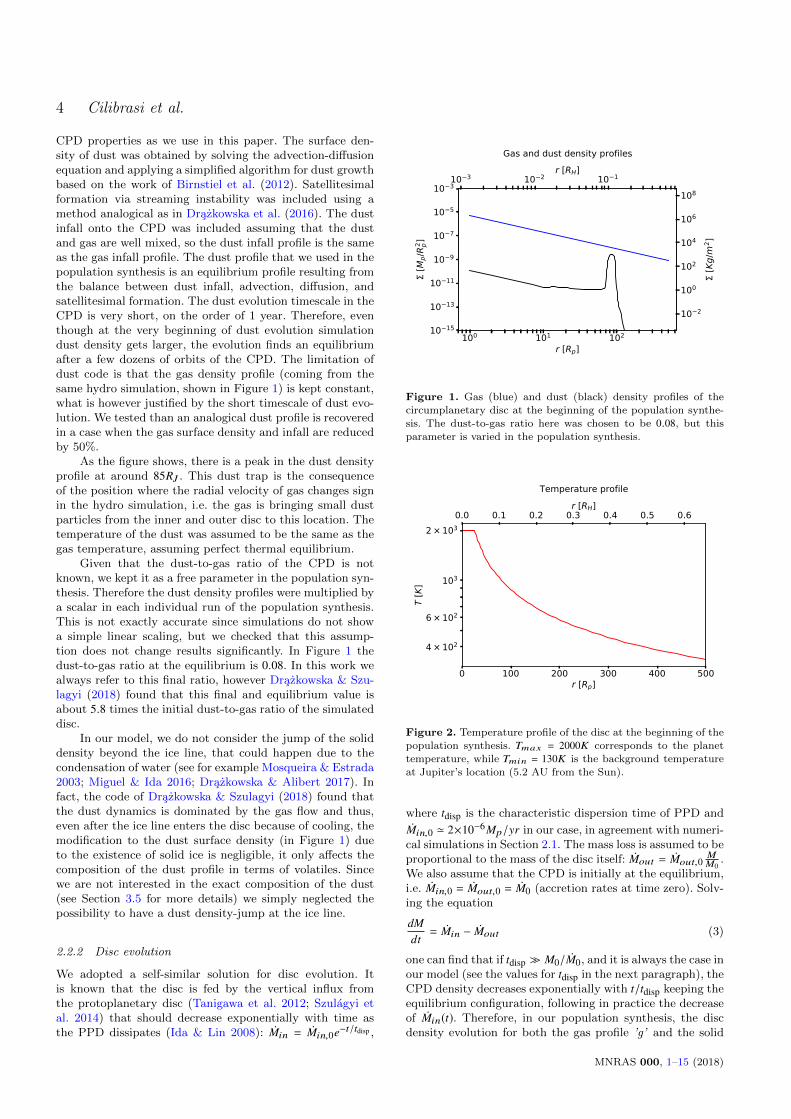
In the model, the CPD is simply defined by its surface den-sity (both solid and gas) profiles, temperature profile andother quantities, such as α for viscosity, γ for heat capacityratio and CV for heat capacity at constant volume. All otherquantities in the disc, such as the angular velocity of the gas,the height of the disc, the speed of sound, etc., are computedstarting from temperature and density values and using thecommon 1D model for discs (Pringle 1981). The disc rangesbetween 1Rp and 500Rp, according to the hydrodynamicalsimulation, and it is divided in 500 cells. In our model we donot consider a cavity between the planet’s surface and thedisc, because the magnetic field of the planet and the ioniza-tion of the disc are probably not strong enough to producesuch a cavity (see also in Section 4). The disc initial tem-perature and gas density profiles are power-law fits to theresults of a radiative hydrodynamical simulation of Szulagyi(2017) with planet temperature of 2000 K (i.e. a late time inthe evolution of the forming planet & its disc, correspondingto roughly 1-2 Myrs of PPD age), described in Section 2.1.The power-laws are the followings (Figure 1, Figure 2):

Σgas(r) ' 4.8 · 10−6(

rRp

)−1.4[

Mp

R2p

](1)

T(r) =

1.4 · 104

(rRp

)−0.6[K] Tmin < T < Tmax

Tmin T ≤ Tmin

Tmax T ≥ Tmax

(2)

with Tmin = 130 K, that is the background temperature inthe PPD at Jupiter’s location like e.g. in Miguel & Ida(2016), and Tmax = 2000 K, that is the planet temperature inthe simulations. The total disc mass is M0 ' 2× 10−3Mp, al-ways accordingly to the 3D hydrodynamic simulation. Otherparameters are chosen to be consistent with the hydrody-namic simulation, therefore the viscosity is α = 0.004 and itis considered constant in all the model, the adiabatic indexis γ = 7/5 (i.e. molecular hydrogen) and the heat capacity(CV ) equals to 10.16K J/(KgK), again because of consistencywith the hydro simulation.

Because the hydrodynamical simulation only givesgas density profile, we used the dust density profile ofDrazkowska & Szulagyi (2018). In this work, the dust evolu-tion code was run in a post-processing step, using the same

MNRAS 000, 1–15 (2018)

4 Cilibrasi et al.

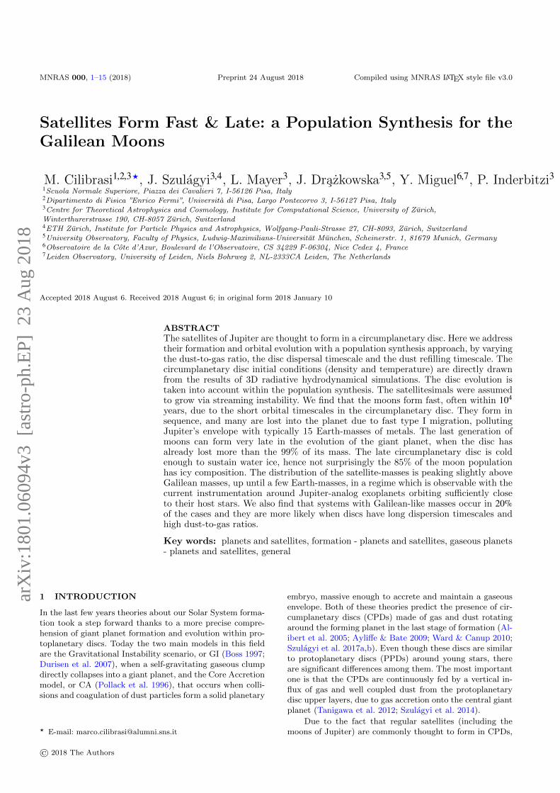
CPD properties as we use in this paper. The surface den-sity of dust was obtained by solving the advection-diffusionequation and applying a simplified algorithm for dust growthbased on the work of Birnstiel et al. (2012). Satellitesimalformation via streaming instability was included using amethod analogical as in Drazkowska et al. (2016). The dustinfall onto the CPD was included assuming that the dustand gas are well mixed, so the dust infall profile is the sameas the gas infall profile. The dust profile that we used in thepopulation synthesis is an equilibrium profile resulting fromthe balance between dust infall, advection, diffusion, andsatellitesimal formation. The dust evolution timescale in theCPD is very short, on the order of 1 year. Therefore, eventhough at the very beginning of dust evolution simulationdust density gets larger, the evolution finds an equilibriumafter a few dozens of orbits of the CPD. The limitation ofdust code is that the gas density profile (coming from thesame hydro simulation, shown in Figure 1) is kept constant,what is however justified by the short timescale of dust evo-lution. We tested than an analogical dust profile is recoveredin a case when the gas surface density and infall are reducedby 50%.

As the figure shows, there is a peak in the dust densityprofile at around 85RJ . This dust trap is the consequenceof the position where the radial velocity of gas changes signin the hydro simulation, i.e. the gas is bringing small dustparticles from the inner and outer disc to this location. Thetemperature of the dust was assumed to be the same as thegas temperature, assuming perfect thermal equilibrium.

Given that the dust-to-gas ratio of the CPD is notknown, we kept it as a free parameter in the population syn-thesis. Therefore the dust density profiles were multiplied bya scalar in each individual run of the population synthesis.This is not exactly accurate since simulations do not showa simple linear scaling, but we checked that this assump-tion does not change results significantly. In Figure 1 thedust-to-gas ratio at the equilibrium is 0.08. In this work wealways refer to this final ratio, however Drazkowska & Szu-lagyi (2018) found that this final and equilibrium value isabout 5.8 times the initial dust-to-gas ratio of the simulateddisc.

In our model, we do not consider the jump of the soliddensity beyond the ice line, that could happen due to thecondensation of water (see for example Mosqueira & Estrada2003; Miguel & Ida 2016; Drazkowska & Alibert 2017). Infact, the code of Drazkowska & Szulagyi (2018) found thatthe dust dynamics is dominated by the gas flow and thus,even after the ice line enters the disc because of cooling, themodification to the dust surface density (in Figure 1) dueto the existence of solid ice is negligible, it only affects thecomposition of the dust profile in terms of volatiles. Sincewe are not interested in the exact composition of the dust(see Section 3.5 for more details) we simply neglected thepossibility to have a dust density-jump at the ice line.

2.2.2 Disc evolution

We adopted a self-similar solution for disc evolution. Itis known that the disc is fed by the vertical influx fromthe protoplanetary disc (Tanigawa et al. 2012; Szulagyi etal. 2014) that should decrease exponentially with time asthe PPD dissipates (Ida & Lin 2008): ÛMin = ÛMin,0e−t/tdisp ,

100 101 102

r [Rp]10 15

10 13

10 11

10 9

10 7

10 5

10 3

[Mp/R

2 p]

Gas and dust density profiles

10 2

100

102

104

106

108

[Kg/

m2 ]

10 3 10 2 10 1r [RH]

Figure 1. Gas (blue) and dust (black) density profiles of the

circumplanetary disc at the beginning of the population synthe-sis. The dust-to-gas ratio here was chosen to be 0.08, but this

parameter is varied in the population synthesis.

0 100 200 300 400 500r [Rp]

103

4 × 102

6 × 102

2 × 103

T [K

]

Temperature profile

0.0 0.1 0.2 0.3 0.4 0.5 0.6r [RH]

Figure 2. Temperature profile of the disc at the beginning of the

population synthesis. Tmax = 2000K corresponds to the planet

temperature, while Tmin = 130K is the background temperatureat Jupiter’s location (5.2 AU from the Sun).

where tdisp is the characteristic dispersion time of PPD andÛMin,0 ' 2×10−6Mp/yr in our case, in agreement with numeri-

cal simulations in Section 2.1. The mass loss is assumed to beproportional to the mass of the disc itself: ÛMout = ÛMout,0

MM0

.We also assume that the CPD is initially at the equilibrium,i.e. ÛMin,0 = ÛMout,0 = ÛM0 (accretion rates at time zero). Solv-ing the equation

dMdt= ÛMin − ÛMout (3)

one can find that if tdisp M0/ ÛM0, and it is always the case inour model (see the values for tdisp in the next paragraph), theCPD density decreases exponentially with t/tdisp keeping theequilibrium configuration, following in practice the decreaseof ÛMin(t). Therefore, in our population synthesis, the discdensity evolution for both the gas profile ’g’ and the solid

MNRAS 000, 1–15 (2018)

Formation of the Galilean Satellites 5

(dust) profile ’s’ is given by:Σg = Σg,0e−t/tdisp

Σs = Σs,0e−t/tdisp − A(4)

where tdisp is the dispersion time of the CPD (that is equal tothe dispersion time of the PPD), Σg,0(r) and Σs,0(r) are theinitial density profiles, while A is the dust accreted by theprotosatellites and then regenerated by the refilling mech-anism, as it will be explained in Section 2.2.3. This meansthat, except the term A, both the gas and dust profile willdecrease following a self-similar solution, keeping the shapeshown in Figure 1. It is important here to keep in mind thatthis solution from Ida & Lin (2008) is valid when α param-eter for viscosity is constant, like in our case.

The disc dispersion timescale and the total disc life-time are not the same thing but they are not independentfrom each other as well, hence we also linked them in ourcalculation. Recent observations showed that disc lifetimesdistribute exponentially between 1Myr and 10Myr with acharacteristic age of 2.3Myr (Fedele et al. 2010; Mamajek2009). These surveys have an accreation rate sensitivity limittill > 10−11Myr−1, however, on average, young T Tauristars with a protoplanetary disc show an accretion rate of∼ 10−7Myr−1 (e.g. Ercolano et al. 2014). Considering theselimits, and considering the exponential evolution of disc den-sity (and mass), the disc lifetime will be:

tlifetime = −tdisp ln(

10−11Myr−1

10−7Myr−1

)' 10tdisp (5)

where the dispersion timescales are distributed exponen-tially between 0.1Myr and 1.0Myr, with a mean of 0.23Myr.

The temperature evolution was calculated also with anexponential decrease to be consistent with the density evo-lution:

T = Tmin + (T0 − Tmin)e−t/tcool (6)

where tcool is computed with the radiative cooling formulaof Wilkins & Clarke (2012):

ÛT ∝ ÛU = −σT4 − T4

min

Σg(τ + τ−1)(7)

The optical depth (τ) can be estimated as τ =∫ρκdh ' κΣg,

where κ(Σ,T) is the opacity computed with tables in Zhu etal. (2009), that are based on a ISM mean dust-to-gas ratio of1%, that is kept constant in this temperature evolution cal-culation, i.e. we do not consider depletion because of satelliteaccretion. This choice was made because the initial dust-to-gas ratio in the CPD is highly unknown, furthermore, thedust density is highly variable during the evolution of a sys-tem. We also tried to add viscous heating in the coolingmodel (CV

ÛT = αc2sΩ, but since it did not change the result

significantly, we omitted it in the final runs to save compu-tational time.)

As the optical depth (τ) depends only on T and Σ, there-fore the cooling depends only on how Σ varies with time, andit is possible to find a relation between the cooling timescaletcool and tdisp (Fig. 3). We define tcool as the time at which thetotal internal energy of the disc divided by the total massof the disc itself (T ∝ U/M) is 1/e of its initial value, as itcan be seen in Figure 4, where it is also clear the exponen-

105 106

tdisp [yr]

2 × 105

3 × 105

4 × 105

6 × 105

t coo

l [yr

]

temperature timescale vs dispersion timetimefit

Figure 3. Relation between tcool and tdisp. The blue dots are the

result for 15 different values of tdisp while the orange line is the fitgiven by equation 8.

0.00 0.25 0.50 0.75 1.00 1.25 1.50 1.75 2.00t [yr] 1e5

106

2 × 106

u [R

2 p/y

r2 ]

Energy per unit mass (u = U/M) vs time, tdisp = 105yr

u(t)u(t = 0)/e

Figure 4. Energy per unit mass u in case of tdisp = 105yr . The

orange line present the initial value for energy divided by e and

the blue line is the energy evolution (cooling). The cooling-curve(blue) is nearly exponential.

tial nature of the cooling process. This relation is found byfitting the results with tdisp between 105yr and 106yr:

log10(tcool) = −0.11log10(tdisp)2 + 1.9log10(tdisp) − 1.5 (8)

where timescales are in years. We also show this fit in Figure3.

The choice of using a ISM mean dust-to-gas ratio is ofcourse an approximation and our results can also be incon-sistent when the dust-to-gas ratio is changed. On the otherhand, since we obtained a value for tcool that is comparableto tdisp, the dispersion of the disc would be the dominanteffect and therefore, a deeper study would not significantlychange our model and outcome.

MNRAS 000, 1–15 (2018)

6 Cilibrasi et al.

2.2.3 Protosatellite formation and evolution

Satellite Formation and Loss Once a simulation hasstarted, the code starts to create a new embryo in the posi-tion of the dust trap, assuming that the mechanism for dustcoagulation is streaming instability (Youdin & Goodman2005), i.e. a mechanism in which the drag felt by solid parti-cles orbiting in a gas disc leads to their spontaneous concen-tration into clumps which can gravitationally collapse. Themoonlet formation process starts when these two conditionsoccur:

(i) The ratio between the solid density and the gas den-sity in the midplane of the dust trap is more than 1. Thiscondition can occur only if the global dust-to-gas ratio ishigh enough (≥ 0.03 is the threshold in the model, i.e. theinitial dust-to-gas ratio should be ≥ 0.005). This value isgiven by the profile definition in Section 2.2.1.

(ii) The previous proto-moon is far enough, i.e. the dusttrap is out of its feeding zone, because of migration.

Once these two conditions have occurred the embryo has togrow to the fixed initial mass (m0 = 10−7Mp, that is morethan two orders of magnitude smaller than individual massesof the Galilean satellites). We use also a formation rate ( Ûm0)taken from Drazkowska & Szulagyi (2018), which we assumeto decrease at the same rate as the circumplanetary disc den-sity decreases, i.e. Ûm = Ûm0e−t/τ . Starting from the momentin which the two above-mentioned conditions occur we inte-grate this formation rate in time until m = m0. At this pointthe code creates the new protosatellite in the disc. The valuefor m0 is arbitrary and we tested various m0 to make surethat this initial parameter does not affect results.

The evolution of a protosatellite is stopped in two oc-casions:

(i) When a protosatellite reaches the inner boundaries ofthe disc, then the satellite is considered to be lost into theplanet.

(ii) When two protosatellites intersect their paths thecode stops the smallest of the two, even if this very rarelyhappens. (We are neglecting the possibility that 2 satellitespass each other in 3D.)

Each simulation ends when the total lifetime of the discis reached, i.e. when t

tdisp∼ 10 (see in Section 2.2.2).

Migration In our model the orbits of the formed satel-lites are always considered circular and coplanar (Moraeset al. 2017) and orbital radii change because of the in-teraction between the disc and the satellites. In the codewe distinguish between type I migration and type II mi-gration. Gap opening separates the two regimes, thereforewe use the gap opening parameter P = 3

4hRH+ 50

q Re =

34

csΩK a

(Ms

3Mp

)−1/3+ 50αMp

Ms

(csΩK a

)2from Crida & Morbidelli

(2007). We consider that type I takes place if P > 1, oth-erwise (if P < 1) type II operates. In the above formula his the scale-height of the disc, RH is the Hill radius of thesatellite, q = Ms/Mp, Re is the Reynolds number, a is thedistance from the central planet, cs is the speed of sound,ΩK is the keplerian velocity at the satellite position.

To compute type I migration velocity we use

vr = bIMsΣga3

M2p

( ah

)2ΩK (9)

where bI is a parameter that is widely used in the migra-tion community and has been computed in different discconditions (Paardekooper et al. 2011; D’Angelo & Lubow2010; Dittkrist et al. 2014). In our code we use the bI ob-tained in 3D non-isothermal simulations in Paardekooper etal. (2011), as a function of the disc density, temperature andsatellite mass. One has also to consider the fact that when asatellite is growing, it is also starting to open a partial gap,therefore the gas density is decreasing in the closer Lindbladlocations and as a consequence, migration velocity decreases.This is done by multiplying bI by the value of the gap depth(0 ≤ depth ≤ 1) according to the analytic formula of Duffell(2015).

In type II migration, the satellite migrates with the gap,with velocity computed as in Pringle (1981):

vr = −3(βΣ + βT + 2)αcsha

(10)

where βΣ = −dlnΣgdlnr and βT = − dlnT

dlnr , or vr = − 32αcsha in

steady state discs, from which it is possible to define a second

b parameter, i.e. bI I = − 32

c4sα

Ω4K a6ΣgMs

. We also want to under-

line that bI I becomes smaller by a factor of ∼ Ms/(4πa2Σg)when the satellite grows in mass (Syer & Clarke 1995) andchanges migration regime (from disc-dominated to satellite-dominated). So we modify bI I as:

bI I → bI I1 + Ms

B

, B = 4πa2Σg (11)

Furthermore, we also considered a smooth transitionbetween type I and type II migration by using a junctionfunction z from Dittkrist et al. (2014):

b = z (1/P) bI + [1 − z (1/P)] bI I (12)

where z(x) = 11+x30 and P is the gap opening parameter de-

fined before.Since the Galilean satellites are found in resonances, we

also tried to resonant trapping in our population synthesis.Actually, the resonance capturing turned out to be a veryrare phenomenon in our model because the inner satellitehas to slow down significantly for capture to occur, becauseit is necessary to have converging orbits. The only strongslowing mechanism in our model would be the gap opening,but as we show in Section 3.3, this happens very rarely.

The migration rates are also used to compute thetime-steps in the code. In more detail, the time-steps arenever longer than tdisp/100 in order not to lose precision onthe disc evolution. Moreover, we also impose that a satel-lite should never move for more than one tenth of a disccell (i.e. 1Rp/10) during its migration. As a consequenceeach timestep is the minimum value between tdisp/100 and0.1Rp/|vmig |, computed separately for each migrating satel-lite.

MNRAS 000, 1–15 (2018)

Formation of the Galilean Satellites 7

Accretion While a protosatellite is migrating in the CPD,it also accretes mass from the dust disc. For a very thin dustdisc this accretion prescription is (Greenberg et al. 1991):

ÛMs = 2Rs Σs

√GMs

Rsv2K

vK = 2(

Rs

a

)1/2Σsa2

(Ms

Mp

)1/2ΩK (13)

where Rs is the radius of the satellite. In the formula, weuse Σs (that is different from Σs), because it is the averagesolid density over the entire feeding zone. The radius of thefeeding zone is the same order of magnitude as the Hill-radius, i.e. Rf = 2.3RH (Greenberg et al. 1991). This valueis then multiplied by the gap depth because if the dust iswell coupled with the gas (i.e. it is composed by small, ≤mm, grains), then as the satellite grows and opens a gap,there will be less dust around it to accrete.

Once a satellite has accreted the computed mass duringa time-step, it is necessary to subtract this mass from thedust disc density. This dust is taken from the feeding zoneproportionally to the available mass in each cell: in eachpoint i of the grid within Rf solid density decreases by a

value of ∆M(i) = Mmax (i)∑Rfi Mmax (i)

dM where Mmax(i) is the mass

available in the i-th cell. It often happens that a moonletaccretes all the mass available in the feeding zone, reachingits isolation mass.

After a protosatellite has accreted the mass in the feed-ing zone and created a gap in the dust, the disc tends touse the dust falling from the PPD’s vertical influx to reachthe equilibrium again (Figure 1), according to Drazkowska& Szulagyi (2018), where the accretion rate onto the centralplanet, plus the dust lost by satellite accretion in our case, isequal to the dust infall rate. In practice, going back towardsthe equilibrium configuration means that dust should fill thedust gaps left by satellite accretion. In the population syn-thesis, we model this refilling mechanism assuming a typicaltimescale trefilling for this process, that could cover a widerange of values, since the dust-to-gas ratio within the ver-tical influx of material is unknown. In our model the CPDgains mass in the following way from the vertical influx:

∆Σs =

Σs−Σstrefilling

dt dt ≤ trefilling

Σs − Σs dt > trefilling(14)

where dt stands for the time-step, Σs is the current soliddensity and Σs is the value that the solid density would haveif there was not accretion and consequent depletion.

The timescale of this process is not well constrained,because it strongly depends, for instance, on the amountof dust that fall into the CPD from the PPD, that can beeither very fast, with trefilling ∼ 102yr, or very slow, with

trefilling ∼ 106yr.

2.2.4 Population synthesis

The last module of the code allows to run the semi-analyticalalgorithm with a population synthesis approach. The ideaof population synthesis is to explore a range of the uncon-strained parameters, trying all the different combinationsbetween them and in the end to compare the results, individ-ually or grouped. The parameters we vary in the populationsynthesis are:

• the dust-to-gas ratio in (0.03, 0.50), changing only thedust component• the CPD dispersion timescale: tdisp in (105, 106)yr• the dust refilling timescale: trefilling in (102, 106)yr

In random cases we distribute tdisp exponentially, as de-scribed by Fedele et al. (2010), while we distribute dust-to-gas ratio and trefilling logarithmically. Furthermore, we varywhen the simulation begins, in order to have different initialconditions in temperature and density profiles of the disc.The simulation can start anytime between 0 and tdisp/2.

In principle one can set lower dust-to-gas ratios butsince streaming instability is only occurring when the dust-to-gas ratio is > 0.03 we did not consider those low dust-to-gas ratio cases in our results. There will be, of courses, caseswith dust-to-gas ratios < 0.03 but estimating their numberwould be possible only when the global dust-to-gas ratio dis-tribution will be clear. For instance, calling the dust-to-gasratio variable x, if we assume a logarithmic probability dis-tribution within 0.01 < x < 0.50, i.e. dp/dx ∝ 1/x, and weextend the distribution in order to go to 0 for low dust-to-gas ratios (for example dp/dx ∝ 100x in 0 < x < 0.01 seemsreasonable), we find that about 35% of the cases have dust-to-gas ratio < 0.03.

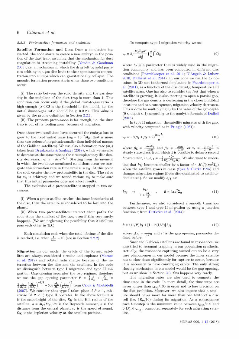
One could also vary other parameters, such as the ini-tial embryos mass or the type I migration formula used. Wetested these, but this did not change the results much, there-fore we kept them fixed as described in the previous sections.We show in Figure 5 how the results of a single run look,with satellites growing, being lost and migrating within aCPD. We also note that there are parameters we kept fixedto be consistent with the hydrodynamic simulation, but theycould have been varied too.

3 RESULTS

In our work we used two kinds of approaches for populationsynthesis: the first one consists in running twenty-thousandsof different simulations with randomizing the three initialparameters described in the previous section. The secondapproach is controlling a value for a single parameter, andlet the other two vary randomly. The first approach allowsto have a general understanding of the outcomes, respectingparameter distribution (especially the exponential distribu-tion of tdisp, that is an observational constraint), while thesecond approach allows to understand how a single param-eter affects the results.

3.1 Survival timescale of the last generation ofsatellites

Due to the fact that the moonlets migrate inwards in thedisc (see Section 3.3), and it is often assumed that there isno cavity between the planet and the CPD (see e.g. Owen &Menou 2016 and Szulagyi & Mordasini 2017), many (even adozen of) satellites are lost into the planet during disc evo-lution and therefore only the latest set of moons will survivewhen the CPD (and PPD) dissipates. This is called sequen-tial satellite formation, that was already suggested in e.g.Canup & Ward (2002). These lost satellites pollute the en-velope of the forming giant planet, increasing the metallicity

MNRAS 000, 1–15 (2018)

8 Cilibrasi et al.

time [yr]0.0

0.2

0.4

0.6

0.8

Orbi

tal r

adiu

s [R P

]

1e2Migration of satellites

0.0 0.5 1.0 1.5 2.0 2.5 3.0time [yr] 1e6

10 7

10 6

10 5

10 4

Sate

llite

mas

s [M

P]

Accretion of satellites

Figure 5. Evolution of satellites in a system with dust-to-gasratio = 0.1, tdisp = 105 yr and trefilling = 2 × 104 yr. Solid lines are

the surviving satellites, dashed lines are lost ones.

10 7 10 6 10 5 10 4 10 3 10 2

Satellite mass [Mp]

10 4

10 3

10 2

10 1

100

101

Lost

mas

s [M

p]

Total lost mass vs total satellites mass

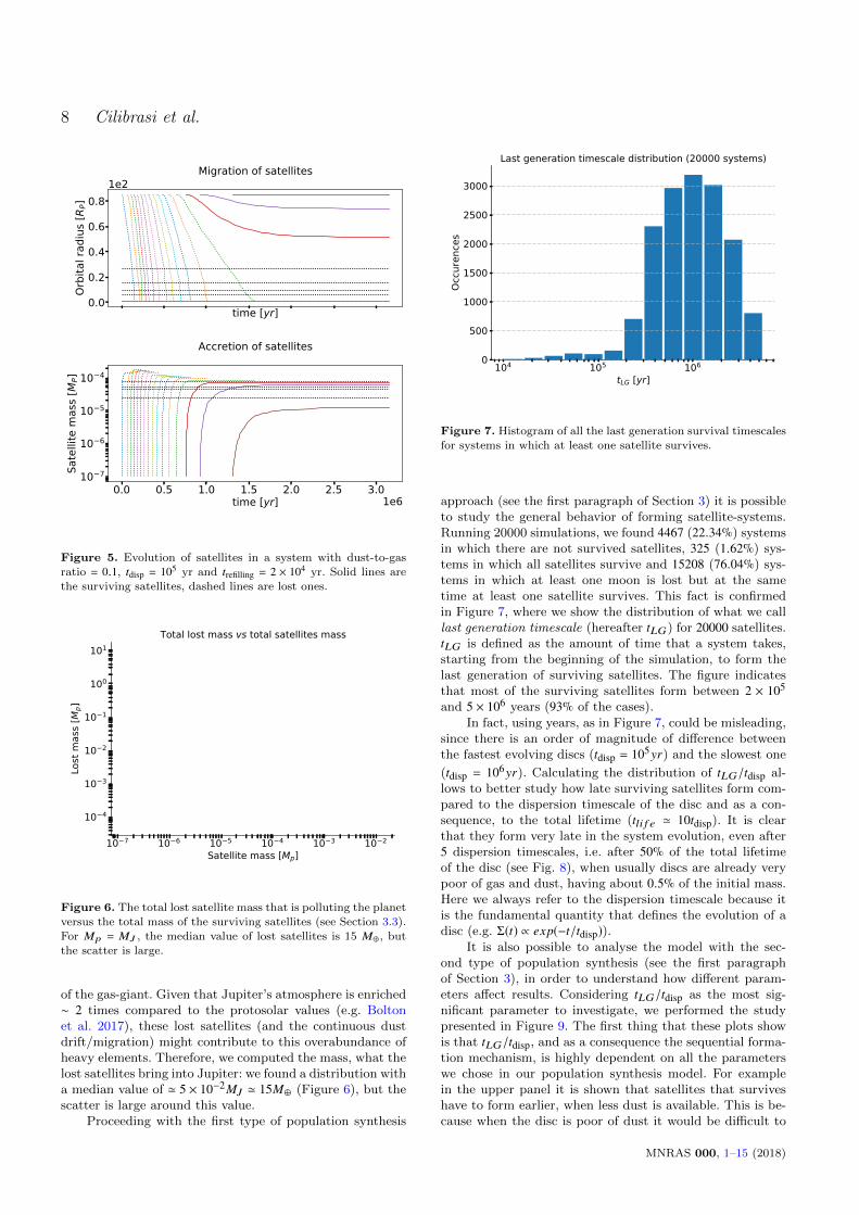
Figure 6. The total lost satellite mass that is polluting the planet

versus the total mass of the surviving satellites (see Section 3.3).For Mp = MJ , the median value of lost satellites is 15 M⊕, butthe scatter is large.

of the gas-giant. Given that Jupiter’s atmosphere is enriched∼ 2 times compared to the protosolar values (e.g. Boltonet al. 2017), these lost satellites (and the continuous dustdrift/migration) might contribute to this overabundance ofheavy elements. Therefore, we computed the mass, what thelost satellites bring into Jupiter: we found a distribution witha median value of ' 5 × 10−2MJ ' 15M⊕ (Figure 6), but thescatter is large around this value.

Proceeding with the first type of population synthesis

104 105 106

tLG [yr]0

500

1000

1500

2000

2500

3000

Occu

renc

es

Last generation timescale distribution (20000 systems)

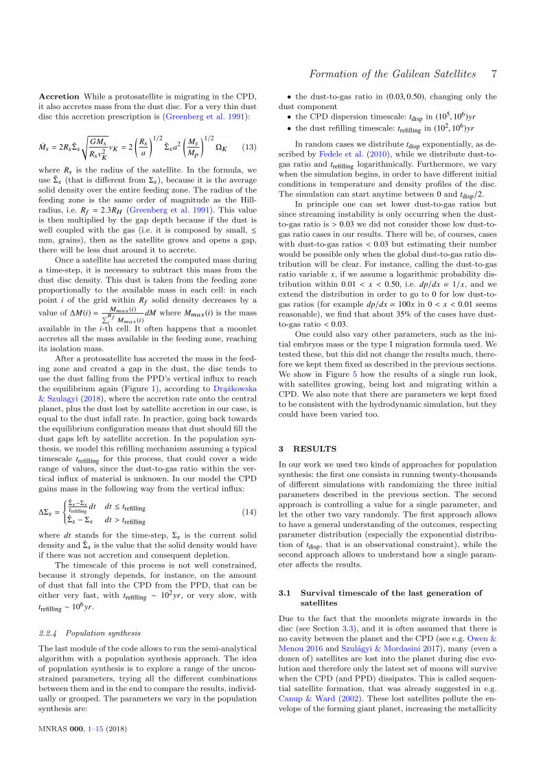
Figure 7. Histogram of all the last generation survival timescales

for systems in which at least one satellite survives.

approach (see the first paragraph of Section 3) it is possibleto study the general behavior of forming satellite-systems.Running 20000 simulations, we found 4467 (22.34%) systemsin which there are not survived satellites, 325 (1.62%) sys-tems in which all satellites survive and 15208 (76.04%) sys-tems in which at least one moon is lost but at the sametime at least one satellite survives. This fact is confirmedin Figure 7, where we show the distribution of what we calllast generation timescale (hereafter tLG) for 20000 satellites.tLG is defined as the amount of time that a system takes,starting from the beginning of the simulation, to form thelast generation of surviving satellites. The figure indicatesthat most of the surviving satellites form between 2 × 105

and 5 × 106 years (93% of the cases).In fact, using years, as in Figure 7, could be misleading,

since there is an order of magnitude of difference betweenthe fastest evolving discs (tdisp = 105yr) and the slowest one

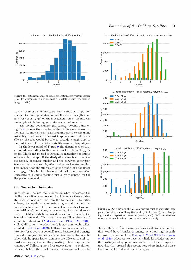
(tdisp = 106yr). Calculating the distribution of tLG/tdisp al-lows to better study how late surviving satellites form com-pared to the dispersion timescale of the disc and as a con-sequence, to the total lifetime (tli f e ' 10tdisp). It is clearthat they form very late in the system evolution, even after5 dispersion timescales, i.e. after 50% of the total lifetimeof the disc (see Fig. 8), when usually discs are already verypoor of gas and dust, having about 0.5% of the initial mass.Here we always refer to the dispersion timescale because itis the fundamental quantity that defines the evolution of adisc (e.g. Σ(t) ∝ exp(−t/tdisp)).

It is also possible to analyse the model with the sec-ond type of population synthesis (see the first paragraphof Section 3), in order to understand how different param-eters affect results. Considering tLG/tdisp as the most sig-nificant parameter to investigate, we performed the studypresented in Figure 9. The first thing that these plots showis that tLG/tdisp, and as a consequence the sequential forma-tion mechanism, is highly dependent on all the parameterswe chose in our population synthesis model. For examplein the upper panel it is shown that satellites that surviveshave to form earlier, when less dust is available. This is be-cause when the disc is poor of dust it would be difficult to

MNRAS 000, 1–15 (2018)

Formation of the Galilean Satellites 9

0 1 2 3 4 5tLG/tdisp

0

500

1000

1500

2000

2500

Occu

renc

es

Last generation ratio distribution (20000 systems)

Figure 8. Histogram of all the last generation survival timescales

(tLG) for systems in which at least one satellite survives, dividedby tdisp (ratio).

reach streaming instability conditions in the dust trap, thenwhether the first generation of satellites survives (then wehave very short tLGs) or the first generation is lost into thecentral planet, following generations can not survive.

The second dependence (i.e. trefilling, second panel onFigure 9), shows that the faster the refilling mechanism is,the later the moons form. This is again related to streaminginstability conditions in the dust trap because if refilling isefficient the disc would be able to provide enough dust tothe dust trap to form a lot of satellites even at later stages.

In the lower panel of Figure 9 the dependence on tdispis plotted. According to this, satellites form later if tdisp islonger. This is not related to streaming instability conditionsas before, but simply if the dissipation time is shorter, thegas density decreases quicker and the survived generationforms earlier. because migration and accretion stop earlier.This means that the timescales of the model are not linearwith tdisp. This is clear because migration and accretiontimescales of a single satellite just slightly depend on thedissipation timescale.

3.2 Formation timescales

Since we still do not really know on what timescales theGalilean satellites were formed, i.e. how much time a satel-lite takes to form starting from the formation of its initialembryo, the population synthesis can give a hint about this.Formation timescales have an impact on the structure andcomposition of the moons, or in reverse, the internal struc-tures of Galilean satellites provide some constraints on theformation timescale. The three inner satellites show a dif-ferentiated structure (Anderson et al. 1996, 1998, 2001),while Callisto, on the other hand, is not completely differ-entiated (Sohl et al. 2002). Differentiation occurs when asatellites (or a body, in general) melts because of the energyreceived from gas interactions, satellitesimals collisions, etc.When this happens heavy elements are allowed to sink to-ward the centre of the satellite, creating different layers. Thestructure of Callisto gives a first caveat about its evolution,i.e. some believe that its formation timescale could not be

0 1 2 3 4 5tLG/tdisp

0

100

200

300

400

Occu

renc

es

tLG ratio distribution (7500 systems), varying dust-to-gas ratio3.7e-02 1.4e-01 5.0e-01

0 1 2 3 4 5tLG/tdisp

0

100

200

300

400

500

600

700Oc

cure

nces

tLG ratio distribution (7500 systems), varying trefilling

1.0e+02 yr1.0e+04 yr1.0e+06 yr

0 1 2 3 4 5tLG/tdisp

0

100

200

300

400

500

600

Occu

renc

es

tLG ratio distribution (7500 systems), varying tdisp

1.0e+05 yr3.2e+05 yr1.0e+06 yr

Figure 9. Distributions of tLG/tdisp varying dust-to-gas ratio (top

panel), varying the refilling timescale (middle panel), and chang-ing the disc dispersion timescale (lower panel). 2500 simulationswere run for each value (7500 simulations in total).

shorter than ∼ 105yr because otherwise collisions and accre-tion would have transferred energy at a rate high enoughto have complete melting (Canup & Ward 2002; Stevensonet al. 1986). However we have very little knowledge on howthe heating/cooling processes worked in the circumplane-tary disc that created this moon, nor, where inside the discCallisto has formed and how its migrated.

MNRAS 000, 1–15 (2018)

10 Cilibrasi et al.

103 104 105 106

Formation timescale [yr]0

1000

2000

3000

4000

5000

6000

7000

8000

Occu

renc

es

Galilean timescale distribution (20000 systems)

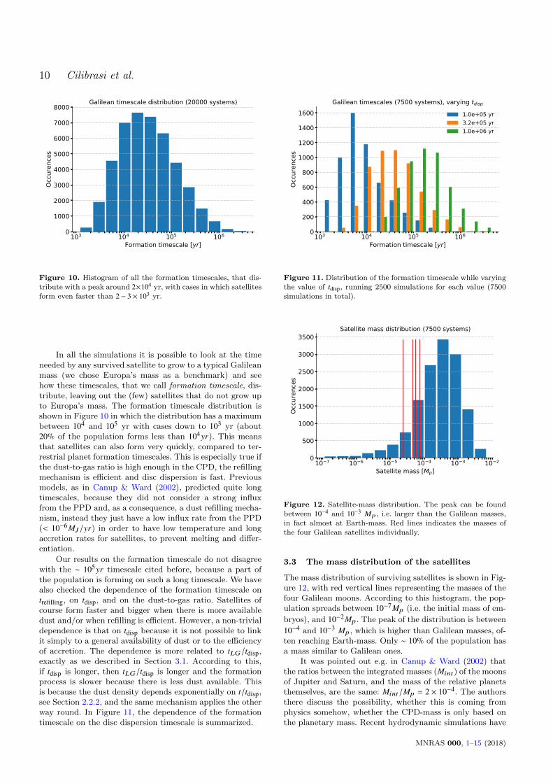
Figure 10. Histogram of all the formation timescales, that dis-

tribute with a peak around 2×104 yr, with cases in which satellitesform even faster than 2 − 3 × 103 yr.

In all the simulations it is possible to look at the timeneeded by any survived satellite to grow to a typical Galileanmass (we chose Europa’s mass as a benchmark) and seehow these timescales, that we call formation timescale, dis-tribute, leaving out the (few) satellites that do not grow upto Europa’s mass. The formation timescale distribution isshown in Figure 10 in which the distribution has a maximumbetween 104 and 105 yr with cases down to 103 yr (about20% of the population forms less than 104yr). This meansthat satellites can also form very quickly, compared to ter-restrial planet formation timescales. This is especially true ifthe dust-to-gas ratio is high enough in the CPD, the refillingmechanism is efficient and disc dispersion is fast. Previousmodels, as in Canup & Ward (2002), predicted quite longtimescales, because they did not consider a strong influxfrom the PPD and, as a consequence, a dust refilling mecha-nism, instead they just have a low influx rate from the PPD(< 10−6MJ/yr) in order to have low temperature and longaccretion rates for satellites, to prevent melting and differ-entiation.

Our results on the formation timescale do not disagreewith the ∼ 105yr timescale cited before, because a part ofthe population is forming on such a long timescale. We havealso checked the dependence of the formation timescale ontrefilling, on tdisp, and on the dust-to-gas ratio. Satellites ofcourse form faster and bigger when there is more availabledust and/or when refilling is efficient. However, a non-trivialdependence is that on tdisp because it is not possible to linkit simply to a general availability of dust or to the efficiencyof accretion. The dependence is more related to tLG/tdisp,exactly as we described in Section 3.1. According to this,if tdisp is longer, then tLG/tdisp is longer and the formationprocess is slower because there is less dust available. Thisis because the dust density depends exponentially on t/tdisp,see Section 2.2.2, and the same mechanism applies the otherway round. In Figure 11, the dependence of the formationtimescale on the disc dispersion timescale is summarized.

103 104 105 106

Formation timescale [yr]0

200

400

600

800

1000

1200

1400

1600

Occu

renc

es

Galilean timescales (7500 systems), varying tdisp

1.0e+05 yr3.2e+05 yr1.0e+06 yr

Figure 11. Distribution of the formation timescale while varying

the value of tdisp, running 2500 simulations for each value (7500simulations in total).

10 7 10 6 10 5 10 4 10 3 10 2

Satellite mass [Mp]0

500

1000

1500

2000

2500

3000

3500

Occu

renc

es

Satellite mass distribution (7500 systems)

Figure 12. Satellite-mass distribution. The peak can be found

between 10−4 and 10−3 Mp , i.e. larger than the Galilean masses,in fact almost at Earth-mass. Red lines indicates the masses of

the four Galilean satellites individually.

3.3 The mass distribution of the satellites

The mass distribution of surviving satellites is shown in Fig-ure 12, with red vertical lines representing the masses of thefour Galilean moons. According to this histogram, the pop-ulation spreads between 10−7Mp (i.e. the initial mass of em-

bryos), and 10−2Mp. The peak of the distribution is between

10−4 and 10−3 Mp, which is higher than Galilean masses, of-ten reaching Earth-mass. Only ∼ 10% of the population hasa mass similar to Galilean ones.

It was pointed out e.g. in Canup & Ward (2002) thatthe ratios between the integrated masses (Mint) of the moonsof Jupiter and Saturn, and the mass of the relative planetsthemselves, are the same: Mint/Mp = 2 × 10−4. The authorsthere discuss the possibility, whether this is coming fromphysics somehow, whether the CPD-mass is only based onthe planetary mass. Recent hydrodynamic simulations have

MNRAS 000, 1–15 (2018)

Formation of the Galilean Satellites 11

10 6 10 5 10 4 10 3 10 2

Integrated mass [Mp]0

500

1000

1500

2000

2500

3000

3500

Occu

renc

es

Integrated mass distribution (20000 systems)

Figure 13. Satellites integrated mass distribution. It has a peak

between 10−4 and 10−3 Mp , while the upper limit is about 10−1Mp .The distribution is symmetric. Red line is the Galilean satellites’

integrated mass (' 2 × 10−4Mp).

shown, however, that not only the planetary mass sets theCPD-mass, but also the PPD-mass, since the latter con-tinuously feeds the former, hence the more massive PPDwill produce a more massive CPD around the same massiveplanet (Szulagyi 2017). To check those results with popu-lation synthesis, in Figure 13 we plotted the histogram ofthe integrated mass of moons in each individual system ofthe population. The vertical red line again highlights theGalilean integrated satellite mass: (2 × 10−4MJupiter). Fromthe Figure it can be concluded that the integrated mass ofsatellites has a wide distribution, there is no hint for anyphysical law producing a peak at Mint = 2 × 10−4Mp, or atany other particular mass. We therefore conclude, that it isjust a coincidence, why the integrated mass of satellites ofJupiter and Saturn are 2 × 10−4Mp.

We also checked in how many cases, out of the total20 thousands, we get systems with 3 or 4 satellites with atotal mass between 10−4Mp and 4 × 10−4Mp, i.e. systemsthat have masses similar to the Galilean ones. We foundthat about 4200 systems have such characteristic, i.e. about21% of the cases. It is easier to have such systems when thedispersion time of the disc is as long as possible (→ 106yr)and the refilling timescale is between 104 and 105 year, whilein those cases the value of dust-to-gas ratio can vary in a verywide range (from 5% to 20%).

We also investigated whether moons can open a gap atall in our model. First of all, one can notice that parameter P(see Section 2.2.3) depends only on the mass of the satellite,the temperature of the CPD, and the position of the satellitein the disc. Hence, it is possible to compute the satellite massMs that can open a gap, as an analytic function of r and T .This way we found that in our model it is very difficult toopen a gap at all (Figure 14), as already stated by Moraeset al. 2017. In the best case (low temperature close to thecentral planet) a satellite with Ms ' 10−4Mp is needed, whichis a quite high value considering the masses of the Galileansatellites distribute between 10−5 and 10−4Mp.

100 101 102

r [Rp]

103

T [K

]

log10(Msat/Mp) for gap opening

4.23.63.02.41.81.20.6

0.00.61.2

Figure 14. Threshold mass for gap opening (P < 1) as a function

of T and r . In the best configuration, i.e. low temperature closeto the planet, a quite a big satellite is still needed to open a gap.

0 1 2 3 4 5Number of survived satellites

0

2000

4000

6000

8000

10000

Occu

renc

es

Survived satellites (20000 systems)

Figure 15. Occurrences of systems with certain numbers of satel-

lites. The peak of the distribution is at 3, while the upper limitis at 5. The most peculiar thing is the minimum visible between

1 and 2.

3.4 The number of survived satellites

In Figure 15 we show the satellites that prevail in each oneof the 20000 systems after the gaseous CPD (and the PPD)dissipates. In other words these are the moons that exist inthe system when the gaseous CPD (and the PPD) dissipates.Without gas, the migration stops, therefore the dynamicalevolution of the satellite system has been terminated. Thehistogram in Figure 15 shows that the most common out-come is a system with 3 satellites. The maximum numberof satellites that can be formed in a system is 5. While 4 isthe second most common result, no-survivor case is also fre-quent. The expectation is that the occurrence rate decreaseswith increasing amount of moons, however our results showan intriguing minimum at N = 1 − 2.

To investigate the reason behind the minimum at 1-2satellite masses, we used again the second type of popula-

MNRAS 000, 1–15 (2018)

12 Cilibrasi et al.

0 1 2 3 4 5Number of survived satellites

0

500

1000

1500

2000

2500

Occu

renc

es

Survived satellites (7500 systems), varying trefilling

1.0e+02 yr1.0e+04 yr1.0e+06 yr

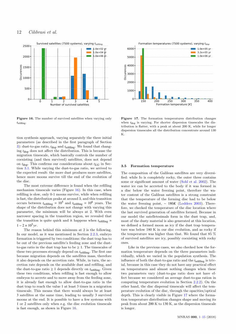
Figure 16. The number of survived satellites when varying only

trefilling.

tion synthesis approach, varying separately the three initialparameters (as described in the first paragraph of Section3): dust-to-gas ratio, tdisp and trefilling. We found that chang-ing tdisp does not affect the distribution. This is because themigration timescale, which basically controls the number ofcoexisting (and then survived) satellites, does not dependon tdisp. This confirms our considerations about tLG in Sec-tion 3.1. While varying the dust-to-gas ratio, we arrived tothe expected result: the more dust produces more satellites,hence more moons survive till the end of the evolution ofthe disc.

The most extreme difference is found when the refillingmechanism timescale varies (Figure 16). In this case, whenrefilling is slow, only 0-1 moons survive, while when refillingis fast, the distribution peaks at around 3, and this transitionoccurs between trefilling = 105 and trefilling = 106 years. Theshape of the distribution does not change with varying thisparameter, the minimum will be always at 2. With evennarrower spacing in the transition region, we revealed thatthe transition is quite quick and it happens when trefilling '1 − 2 × 105yr.

The reason behind this minimum at 2 is the following.In our model, as it was mentioned in Section 2.2.3, embryoformation is triggered by two conditions: the dust trap has tobe out of the previous satellite’s feeding zone and the dust-to-gas ratio in the dust trap has to be ≥ 1. The timescales ofthese two processes strongly depend on trefilling. The first onebecause migration depends on the satellites mass, thereforeit also depends on the accretion rate. While, in turn, the ac-cretion rate depends on the available dust and refilling, andthe dust-to-gas ratio ≥ 1 depends directly on trefilling. Giventhese two conditions, when refilling is fast enough to allowembryos to accrete and to move away from the feeding zone,it is already fast enough to allow dust-to-gas ratio in thedust trap to reach the value 1 at least 3 times in a migrationtimescale. This means that there would always be at least3 satellites at the same time, leading to usually 3 survivedmoons at the end. It is possible to have a few systems with1 or 2 satellites only when e.g. the disc evolution timescaleis fast enough, as shown in Figure 16.

150 200 250 300 350 400Formation temperature [K]

0

1000

2000

3000

4000

5000

6000

Occu

renc

es

Formation temperatures (7500 systems), varying tdisp

1.0e+05 yr3.2e+05 yr1.0e+06 yr

Figure 17. The formation temperatures distribution changes

when tdisp is varying. For shorter dispersion timescales the dis-tribution is flatter, with a peak at about 200 K, while for longer

dispersion timescales all the distribution concentrate around 130

K.

3.5 Formation temperature

The composition of the Galilean satellites are very diversi-fied: while Io is completely rocky, the outer three containssome or significant amount of water (Sohl et al. 2002). Thewater ice can be accreted to the body if it was formed ina disc below the water freezing point, therefore the wa-ter content of the Galilean satellites is a strong constraintthat the temperature of the forming disc had to be belowthe water freezing point, ∼ 180K (Lodders 2003). There-fore, we checked the temperature of the disc location wherethe last survived generation of satellites formed. Because inour model the satelletesimals form in the dust trap, and,most of the dusty material is also generated at this location,we defined a formed moon as icy if the dust trap tempera-ture was below 180 K in our disc evolution, and as rocky ifthe temperature was higher than that. We found that 85 %of survived satellites are icy, possibly coexisting with rockyones.

Like in the previous cases, we also checked how the for-mation temperature depends on the three parameters indi-vidually, which we varied in the population synthesis. Theinfluence of both the dust-to-gas ratio and the trefilling is triv-ial, because in this case they do not have any practical effecton temperatures and almost nothing changes when thesetwo parameters vary (dust-to-gas ratio does not have ef-fect because we considered an average dust-to-gas ration incomputing temperature evolution in Section 2.2.2). On theother hand, the disc dispersal timescale will affect the tem-perature evolution of the disc, through the opacities/opticaldepth. This is clearly visible in Figure 17 where the forma-tion temperature distribution changes shape and moving itspeak from about 200 K to 130 K, as the dispersion timescaleis longer.

MNRAS 000, 1–15 (2018)

Formation of the Galilean Satellites 13

4 DISCUSSION

As it is usual in population synthesis, the choices of theparameters, as well as some assumptions on the processesmight change the results. In this Section we will discuss this,and describe tests and their results on the model, underlin-ing also the biases that affect this work.

First of all, the disc structure has been modeled startingfrom the density and temperature profiles in the mid-planeof the disc coming from 3D radiative hydro simulations. Allthe other features of the disc, such as scale-height, pressure,surface density, sound speed, etc., have been computed fromthe 1D disc model (Pringle 1981). This is a first approxi-mation that affects some of the CPD features, such as ra-dial velocity profile, opacity and azimuthal velocity, sincethese quantities strongly depend on, for example, the pres-sure gradient in the mid-plane, that is computed from the1D model. Furthermore, for this particular work we used ahydrodynamical model designed for CPD formation in core-accretion. If the CPD forms via disc instability, its prop-erties would be significantly different, see e.g. Shabram &Boley (2013), Szulagyi et al. (2017a).

Another bias is the disc evolution. For both dispersionand cooling we chose to use self-similar solutions, but, al-though modeling dispersion of the disc in this way is some-thing common and already used in previous satellite popu-lation synthesis works (Ida & Lin 2008; Miguel & Ida 2016),a self-similar solution for cooling was a choice taken in orderto be consistent with the rest of the semi-analytical frame-work, since it is the first time that CPD-cooling is performedin such a model.

Whether or not there is a magnetospheric cavity be-tween the planet and the disc can affect how many moonsare lost in the planet, or whether they could be capturedinto resonance (easily). With no cavity between the planetand the disc, the migration rate of the moons will not beslowed down sufficiently and they will be easily lost in theplanet. If there was a disc inner edge, that could hold the in-ner moons, and, behind, a resonance chain of satellites couldpile up (Sasaki et al. 2010; Ogihara & Ida 2012), like in thecase of Super-Earths in PPDs (Ogihara & Ida 2009). Evenin this case, the torque of the newly formed, outer satel-lites can eventually push the inner moon into the planet.Nevertheless, in this case probably less moons would be lostand more satellites in resonances would be the outcome. Inthe case of stars, due to the very strong magnetic fields,there is a gap between the surface of the star and the innerPPD. However, giant planets have significantly weaker mag-netic fields, Jupiter, for example, has about 7 Gauss today(Bolton et al. 2017). Even though it can be expected, likein the case of stars, that giant planets might have strongermagnetic field during their early years than today, no workhas been carried out on this matter. There might be a scal-ing law between the luminosity and the magnetic field asit was pointed out by Christensen et al. (2009), suggestingthat a luminous planet in its formation phase could havea high magnetic field. On the other hand, Owen & Menou(2016) calculates that Jupiter had to have at least an or-der of magnitude higher magnetic field than it has today,to induce magnetospheric accretion (and have a cavity be-tween the planet and the disc), and the authors state thatit is unlikely that Jupiter ever had such a strong magnetic

field. They conclude, that the boundary layer accretion (i.e.when the disc touches the planet surface, like in our hydro-dynamic simulations) is a more viable solution. Moreover,if the giant planet has a strong magnetic field, in itself thisis not a sufficient condition for magnetospheric accretion tostart. The gas inside the CPD has to be ionized, otherwise,the neutral gas will not care about the magnetic field andwill enter into the cavity region. The ionization fraction ofthe CPD, on the contrary to the inner PPD, is very low asit was found in several works (Szulagyi & Mordasini 2017;Fujii et al. 2011, 2014).

Nevertheless, we checked how the results change whena cavity is assumed between the planet and the disc. In thiscase the first satellite would stop at the edge of the disc. Thefollowing satellite would then approach the first one and itwould possibly be caught in a 2 : 1 resonant configuration.Whether or not this capture happens can be inferred fromanalytical conditions, e.g. in Ogihara et al. (2010). In theirwork they found that, in case of a sharp disc edge and usingthe type I migration formula by D’Angelo & Lubow (2010)for its simplicity (we show below that changing the type Imigration formula does not change our results significantly),up to 3 satellites would be locked in a resonant configurationwhen te/ta < 1.7×10−3, where te is the eccentricity dampingtimescale and ta is the type I migration timescale. In ourcase this criterion implies a condition on the aspect ratioof the disc at the inner edge, i.e. h/r < 0.024. Using thedefinition of h in a 1D disc model (Pringle 1981) one findsthe condition

T[K]

rcavityRp

≤ 210 (15)

where T is the temperature at the inner edge of the disc.This means that if we want to pile satellites up starting fromthe position of Io (' 6Rp) we need to have a temperatureof about 35K, that is unphysical, due to the backgroundtemperature at Jupiter’s location is about 130 K.

Even if building a resonant structure is not possible inour model, we checked how the final results change when acavity (as big as 2.5Rp or 5Rp) is introduced. In this case weconsidered that satellites stop their migration due to gas in-teraction when reaching the inner edge of the disc, but theystill dynamically interact with other satellites. This meansthey still can be lost into the planet. The interaction betweensatellites has been modeled following the approach of Ida &Lin (2010), i.e. considering that satellites tend to enlargetheir orbital distance ∆a at each encounter. As expected,we found that we have more surviving satellites (their meannumber grows from 2.5 in the case without a cavity to 3.8and 4.5 respectively, when the two different cavities are in-troduced) and as a consequence the integrated final moonmass grows from a median value of 6×10−4Mp to 8×10−4Mp

and 12 × 10−4Mp, respectively, while the mean mass of sin-gle satellites does not change significantly (when satellitesstop their migration in the cavity they also stop their accre-tion). Further investigations about surviving and lost satel-lites would need a more precise model for resonance captur-ing and for collisions between satellites, since this would bedominant processes in the satellite evolution.

In this work we also assumed that streaming instabilityforms the seeds of the moons. More conventional approachesbased on collisional coagulation of dust grains would work

MNRAS 000, 1–15 (2018)

14 Cilibrasi et al.

with lower dust-to-gas ratios, but would provide much longerformation timescales. In the latter models it is notoriouslydifficult to overcome the meter-size barrier as well as otherissues. Since our hydrodynamical simulations have showedthat dust traps appear in CPDs, it was natural to assumethat streaming instability can operate. Another mechanism,that could have provided the seeds is the capturing of plan-etesimals from the PPD (D’Angelo & Podolak 2015; Tani-gawa et al. 2014). Given that we found that the CPD is anefficient satelletesimal factory, we believe that there is noneed for planetesimal capturing to form the moons there.

Regarding testing the initial parameters, we firstchecked the effect of initial embryo mass and a differentType I migration formula. In the latter, instead of thePaardekooper-formula (Paardekooper et al. 2011) we testedthe bI coefficient from D’Angelo & Lubow (2010) and Dit-tkrist et al. (2014). Our finding is that the distribution of thepopulation does not change much, the difference is withinthe change that is caused by random variations.

In comparison to the previous satellite population syn-thesis work by Miguel & Ida (2016), our results are some-what different. While the other authors started with a Min-imum Mass Sub-solar Nebula that is created by the currentposition and composition of Galilean moons, we use real hy-drodynamic simulations on the circumplanetary disc as aninitial gas and dust disc. Like them, we take into accountthe disc evolution both in dust and gas density, but we alsoaccount for evolution in the temperature profile, and we donot consider a cavity between the planet and the disc. Theyfound that in the case of long disc lifetimes, the survivedsatellites are less numerous and have lower masses than inour case, since the biggest ones have enough time to migrateand be lost into the central planet. The difference comesfrom the different dust-to-gas ratios, different disc initialparameters, and the assumption on which process gener-ates the seeds of satellites, but also from the fact that theydid not have any dust supply in the disc while accretion onprotosatellites creates gaps in the dust profile. As a conse-quence their protosatellites have less available dust to growto larger sizes.

Comparing also to the previous works by Canup & Ward(2002) and Canup & Ward (2006) we find that our resultsare partially in agreement with their conclusion, but we havealso points of disagreement. First of all we agree that theCPD can in general be less massive than the MMSN model,in the scenario in which the disc itself is continuously fedby the influx from the PPD. We also agree on the fact thatwith our conditions on viscosity (α = 4× 10−3) type I migra-tion should be always inward and on the fact that survivingsatellites should form very late in the evolution of a Jupiter-like planet. On the other hand, we disagree on the fact thatall the satellites should form, or have formed in the specificcase of Jupiter, slowly, in > 105yr.

The requirement of slow formation comes from the needto explain the non-differentiated nature of Callisto. However,in our model, since we can form many generations of satel-lites, up to the time when the disc is already more thana million years old, Callisto can form late and gradually.Furthermore, by starting with planetary cores formed bystreaming instability, collisions between large planetary em-bryos, which would cause melting and differentiation, arenot required to assemble the satellite.

5 CONCLUSION

In this work we investigated the formation and the evolutionof the Galilean satellites in a circumplanetary disc arounda Jupiter-like planet. We used a population synthesis ap-proach involving 20000 systems, using the initial conditions(disc density and temperature profiles) from a 3D radia-tive simulation of Szulagyi (2017), including the continuousfeeding of gas and <mm sized dust from the protoplanetarydisc (Szulagyi et al. 2014). In the population synthesis, weaccounted for the disc evolution and used a dust density pro-file from a realistic dust coagulation model of Drazkowska &Szulagyi (2018). Furthermore, in our model the seeds of themoons form via streaming instability in a dust trap, whoselocation is around 80 RJup based on the vertical velocityprofiles of the hydrodynamic simulation. The satellitesimalsthen migrate, accrete, are captured in resonances and areoften lost in the planet.

Nevertheless, we found that due to the dust trap, andthe continuous influx of dust from the circumstellar disc,massive satellites are forming (the distribution peaks abovethe Galilean mass at ' 3 × 10−4MJ ' MEarth). Due to theirhigh masses, they quickly migrate into the planet via Type Imigration, because in most of the cases the gap opening cri-terion is not satisfied, the migration cannot enter the Type IIregime. This means that the satellites form in sequence, andmany are lost into the central planet polluting its envelopewith metals. Our results show that the moons are formingfast, often within 104 years (20 % of the population), whichis mainly due to the short orbital timescales of the circum-planetary disc. Indeed the CPD completes several ordersof magnitude more revolutions around the planet than theprotoplanetary disc material can do around the star at thelocation of Jupiter. Due to the short formation time, thesatellites can form very late, about 30% after 4 dispersiontimescales, i.e. when the disc has ∼ 2% of the initial mass.Since our model included disc evolution, the CPD cooledoff during this time, allowing to form icy moons, when thedust trap temperature dropped below 180 K, i.e. the waterfreezing point. We found out that about 85% of the survivedmoons could contain water (ice). The production of moon-lets and the migration rate provided such a situation, whenthe number of survived moons peaked around 3, but oftenno moons survived at all.

The lost satellites bring on average 15 Earth-masses intothe giant planet’s envelope, polluting it with metals, that cancontribute to the abundance of heavy elements in Jupiter’senvelope. The high mass satellites we found in our popu-lation synthesis have intriguing implications for the futuresurveys of exomoons. Indeed even with the current instru-mentation, an Earth-mass moon around a Jupiter analogcan be detected if the planet is orbiting relatively close toits star (Kipping 2009).

ACKNOWLEDGMENTS

We are thankful for anonymous referee for their commentsthat helped to clarify the paper. We also thank for theuseful discussions with Yann Alibert, Christoph Mordasini,Clement Baruteau, Willy Kley and Rene Heller. This workhas been in part carried out within the frame of the National

MNRAS 000, 1–15 (2018)

Formation of the Galilean Satellites 15

Centre for Competence in Research “PlanetS” supported bythe Swiss National Science Foundation. J. Sz. acknowledgesthe support from the ETH Post-doctoral Fellowship fromthe Swiss Federal Institute of Technology (ETH Zurich) andthe Swiss National Science Foundation (SNSF) Ambizionegrant PZ00P2 174115. Computations have been done on the“Monch” machine hosted at the Swiss National Computa-tional Centre.

REFERENCES

Alibert, Y., Mousis, O., & Benz, W. 2005, A&A, 439, 1205

Anderson, J. D., Jacobson, R. A., Lau, E., Sjogren, W. L., Schu-bert, G., & Moore, W. B., 1996, Nature, 384, 541

Anderson, J. D., Jacobson, R. A., Lau, E., Sjogren, W. L., Schu-

bert, G., & Moore, W. B., 1998, Science, 5369, 1573

Anderson, J. D., Jacobson, R. A., Lau, E., Moore, W. B., & Schu-

bert, G., 2001, Icarus, 153, 157

Ayliffe, B. A. & Bate, M. R., 2009, Mon. Not. R. Astron. Soc.

397, 657-665

Bell, K. R., & Lin, D. N. C. 1994, ApJ, 427, 987

Benz, W., Ida, S., Alibert, Y., Lin, D., & Mordasini, C., 2014,

Protostars and Planets, VI

Birnstiel, T., Klahr, H., & Ercolano, B., 2012, A&A, 539, A148

Bolton, S. J., Adriani, A., Adumitroaie, V., et al., 2017, Science,

356, 821-825

Boss, A. P., 1997, Science, 276, 5320, 1836-1839

Boulanger, F., Cox, P., & Jones, A. P., 2000, Infrared space as-

tronomy, today and tomorrow, 70, 251

Canup, R. M. & Ward, W. R., 2002, The Astronomical Journal,

124, 3404-3423

Canup, R. M. & Ward, W. R., 2006, Nature, 441, 834-839

Canup, R. M. & Ward, W. R., 2009, Origin of Europa and the

Galilean Satellites, 59

Commercon, B., Teyssier, R., Audit, E., Hennebelle, P., &

Chabrier, G. 2011, A&A, 529, A35

Crida, A. & Morbidelli, A., 2014, Mon. Not. R. Astron. Soc. 377,

1324-1336

Christensen, U. R., Holzwarth, V., & Reiners, A. 2009, Nature,

457, 167

D’Angelo, G. & Lubow, S. H., 2010, ApJ, 724, 730-747

D’Angelo, G., & Podolak, M. 2015, ApJ, 806, 203

de Val-Borro, M., Edgar, R. G., Artymowicz, P., et al. 2006, MN-

RAS, 370, 529

Dittkrist, K.-M., Mordasini, C., Klahr, H., Alibert, Y., & Hen-

ning, T., 2014, Astronomy & Astrophysics, 567, A121

Drazkowska, J., & Szulagyi, J., 2018, ArXiv e-prints,

arXiv:1807.02638

Drazkowska, J., & Alibert, Y., 2017, A&A 608, A92

Drazkowska, J., Alibert, Y., & Moore, B, 2016, A&A 594, A105

Duffell, P. C., 2011, ApJLetters, 807, L11

Durisen, R. H., Boss, A. P., Mayer, L., Nelson, A. F., & Quinn,T., 2007, Protostars and Planets V, 607-622

Ercolano, B., Mayr, D., Owen, J. E., Rosotti, G., & Manara, C.

F., 2014, MNRAS, 439, 256-263

Estrada, P. R., Mosqueira, I., Lissauer, J. J., D’Angelo, G., &Cruikshank, D. P., 2009, in Europa, ed. R. T. Pappalardo,

W. B. McKinnon, & K. Khurana (Tucson, AZ: Univ. ArizonaPress), 27

Fedele, D., van den Ancker, M. E., Henning, T., Jayawardhana,

R., & Oliveira J. M., 2010, A&A 510, A72

Fujii, Y. I., Okuzumi, S., & Inutsuka, S., 2011, ApJ, 743, 53

Fujii, Y. I., Okuzumi, S., Tanigawa, T., & Inutsuka, S., 2014, The

Astronomical Journal, 785, Issue 2

Fujii, Y. I., Kobayashi, H., Takahashi, S. Z., & Gressel, O., 2017,

The Astronomical Journal, 153, Issue 4

Fung, J., & Chiang, E. 2016, ApJ, 832, 105

Galvagni, M. & Mayer, L., 2012, Mon Not R Astron Soc, 427,

1725-1740Greenberg, R., Bottke, W. F., Carusi, A., & Valsecchi, G. B.,

1991, Icarus 94, 98-111

Gressel, O., Nelson, R. P., Turner, N. J., & Ziegler, U., 2013, ApJ,779, 1

Heller, R. & Pudritz, R., 2015a, ApJ, 806, 181

Heller, R. & Pudritz, R., 2015b, A&A, 578, A19Ida, S. & Lin, D. N. C., 2008, ApJ, 673, 487-501

Ida, S. & Lin, D. N. C., 2010, ApJ, 719, 810-830Kipping, D. M., 2009, Mon Not R Astron Soc, 392, 181-189

Kley, W., 1989, A&A, 208, 98

Lodders, K. 2003, ApJ, 591, 1220-1247Mamajek, E. E. 2009, AIP Conference Proceedings, 1158, 3-10

Miguel, Y. & Ida, S., 2016, Icarus, 266, 1-14

Moraes, R. A., Kley, W., & Vieira Neto, E., 2017, Mon Not RAstron Soc, 475, 1347-1362

Mordasini, C., Marleau, G.-D., & Molliere, P., 2017, A&A, 608,

A72Mosqueira, I. & Estrada, P. R., 2003, Icarus, 163, 198-231

Ogihara, M. & Ida, S., 2009, ApJ, 699, 824-838

Ogihara, M., Duncan, M. J., & Ida, S., 2010, ApJ, 721, 1184-1192Ogihara, M. & Ida, S., 2012, ApJ, 753, 60

Owen, J. E., & Menou, K. 2016, ApJ, 819, L14Paardekooper, S.-J., Baruteau, C., & Kley, W., 2011, Mon. Not.

R. Astron. Soc., 410, 293

Pollack, J. B., & Consolmagno, G., 1984, in Saturn, ed. T. Gehrels& M. S. Matthews (Tucson: Univ. Arizona Press), 811

Pollack, J. B., 1996, Icarus, 124, 1, 62-85

Pringle, J. E., 1981, Annual review of astronomy and astrophysics,19, 137-162

Sasaki, T., Stewart, G. R., & Ida, S., 2010, ApJ, 714, 1052-1064

Shabram, M. & Boley, A. C., 2013, ApJ, 767, 63Showman, A. P. & Malhotra, R., 1999, Science, 296, 77-84

Sohl, F., Spohn, T., Breuer, D., & Nagel, K., 2002, Icarus, 157,

104Stevenson, D. J., Harris, A. W., & Lunine, J. I., 1986, Satellites

(A87-23307 09-91), University of Arizona Press, 39-88Syer, D. & Clarke, C. J., 1995, Mon. Not. R. Astron. Soc. 277,

758-766Szulagyi, J., Morbidelli, A., Crida, A., & Masset, J., 2014, ApJ,

782, 65

Szulagyi, J., Masset, F., Lega, E., Crida, A., Morbidelli, A., &

Guillot, T., 2016, Mon. Not. R. Astron. Soc., 460, 2853-2861Szulagyi, J., Mayer, L., Quinn, T., 2017, Mon. Not. R. Astron.

Soc., 464, 3158-3168

Szulagyi, J., & Mordasini, C. 2017, MNRAS, 465, L64Szulagyi, J. 2017, ApJ, 842, 103

Szulagyi, J., van der Plas, G., Meyer, M. R., Pohl, A., Quanz, S.P., Mayer, L., Daemgen, S., & Tamburello, V., 2017, acceptedfor publication at Mon Not R Astron Soc

Tanaka, H., Takeuchi, T., & Ward, W. R., ApJ, 565, 1257

Tanigawa, T., Ohtsuki, & Machida, M. N., 2012, European Plan-etary Science Congress, 7, 610

Tanigawa, T., Maruta, A., & Machida, M. N. 2014, ApJ, 784, 109Ward, W. R. & Canup, R. M., 2010, The Astronomical Journal,

140, 1168-1193

Wilkins, D. R. & Clarke, C. J., 2012, Monthly Notices of theRoyal Astronomical Society, 419, 4, 3368-3377

Youdin, A. N. & Goodman, J., 2005, ApJ, 620, 459-469

Zhu, Z., Hartmann, L., & Gammie, C., 2009, ApJ, 694, 1045-1055

MNRAS 000, 1–15 (2018)