Published by the Association Pro ISSI

No 10, June 2003

INTERNATIONAL SPACESCIENCEINSTITUTE

Satellite Navigation Systems for Earth and Space Sciences

It was in 1915 when the Germanscientist Alfred Wegener pub-lished the “The Origin of Con-tinents and Oceans” outlining theconcept of continental drift forthe first time. According to thistheory, all the continents on Earthhad formed from one single massabout 300 million years ago,calledPangaea. Later on, Pangaea hadsplit, and its pieces had been mov-ing away from each other eversince. Where such continentalplates collide, mountain rangesmay be pushed up, like for exam-ple the Alps that are the collisionproduct of the African and theEurasian plate.

Initially, Wegener’s theory wasstrongly contested not least be-cause he did not provide convinc-ing explanations for the mechan-ics allowing for the movement ofthe continents through the oceans(as it was seen at that time). Todaywe know that below the continen-tal plates there is a hot liquid zone,the asthenosphere, on which thecontinents f loat. The plates areseparated by ridges, where freshmagma spills out from the as-thenosphere providing the thrustto the continental plates movingthem apart thereby.

In the meantime such different sci-entif ic branches as geology, palae-ontology, botany and zoology haveprovided ample proof in supportof Wegener ’s theory. Even spacetechnology has contributed by thedirect measurement of the conti-nental drift.As an example,the driftvelocity between America and Eu-rope has been determined to be inthe order of 2.5 centimetres /year.

Global satellite navigation systemsare based on a constellation ofEarth orbiting spacecraft emittingsignals with precise orbital andtime data. Suitable receiver equip-ment combines the signals from atleast four spacecraft yielding thetime and the three space coordi-nates. The US Global PositioningSystem (GPS) for instance consistsof 24 spacecraft orbiting the Earthin six different planes. The Russ-ian Glonass system as well as theplanned European Galileo systemare based on the same concepts.

Of course, the GPS originally wasnot conceived as a scientif ic toolbut much more as a sophisticatedmilitary infrastructure for the ful-f ilment of navigational tasks. Itwas only after its commissioningthat its scientif ic value became ap-parent. The continental drift ve-locities measurement is just one ofa number of fascinating scientif icapplications of global navigationsystems to which the present issueof Spatium is devoted. We aregreatly indebted to Prof. GerhardBeutler, Astronomical Institute,University of Berne for his kindpermission to publish herewith arevised version of his excitinglecture of November 12, 2002 forthe members of our association.

Hansjörg SchlaepferZürich, June 2003

2SPAT IUM 10

Impressum

SPATIUMPublished by theAssociation Pro ISSItwice a year

Association Pro ISSIHallerstrasse 6,CH-3012 BernPhone +41 (0)3163148 96Fax +41 (0)3163148 97

President Prof.Heinrich Leutwyler,University of BernPublisherDr.Hansjörg Schlaepfer,legenda schläpfer wort & bild,WinkelLayoutMarcel Künzi,marketing · kom-munikation, CH-8483 KollbrunnPrinting Druckerei Peter + Co dpcCH-8037 Zurich

Front Cover: The Galileo naviga-tion satellite in an artist ’s view(credit : European Space AgencyESA)

INTERNATIONAL SPACESCIENCEINSTITUTE

Editorial

3SPAT IUM 10

Navigation andScience in thePast and Today

The introduction to Peter Apian’sGeographia from 1533 in Figure 1nicely illustrates that positioning inthe “good old times” in essencemeant measuring angles – the scalewas eventually introduced by oneknown distance between two sites(as indicated by the symbolicmeasurement rod in the centre ofthe wood-cut).

Figure 1 also shows that relativelocal and absolute positioning wasperformed with the same instru-ments, the so-called cross-staffs, inApian’s days. Global positioningmeant the determination of theobserver’s geographical latitude andlongitude (relative to an arbitrarilyselected site – first Paris, thenGreenwich was used for this pur-pose). The latitude of an observ-ing site was easily established bydetermining the elevation (at theobserver’s location) of the Earth’srotation axis, approximately repre-sented by the polar star. In princi-ple, longitude determination wassimple, as well: One merely had todetermine the time difference (de-

rived either from the Sun [localsolar time] or from the stars [side-rial time]) between the unknownsite and Greenwich. The problemresided in the realisation of Green-wich time at the observing site inthe pre-telecommunication era.One astronomical solution to thisproblem, illustrated in Figure 1,consisted of measuring the so-called lunar distances (angles be-tween bright stars and the Moon).With increasing accuracy of the(prediction of the) lunar orbit theangular distances between theMoon and the stars could be accu-rately predicted and tabulated inastronomical and nautical al-manacs with Greenwich local

Satellite Navigation Systemsfor Earth and Space Sciences *)

Gerhard Beutler, Astronomical Institute, University of Bern

*) Pro ISSI lecture, Bern,12th November 2002

Figure 1Geographia by Peter Apian, dated 1533.

time as argument. Lunar distanceswere used for centuries for precisepositioning. For navigation on seathe method became eventually ob-solete with the development ofmarine chronometers, which werecapable of transporting accuratelyGreenwich time in vessels overtime spans of weeks. Figure 2 showsthe first chronometer developedby the ingenious British watch-maker J.Harrison (1693–1776).

The principles of precise global po-sitioning and precise navigationremained in essence the samefrom Apian’s times till well intothe second half of the 20th century.The development of the accuracywas dramatic: The cross-staff wasreplaced by increasingly more so-phisticated optical telescopes.More precise star catalogues (fun-damental catalogues) were pro-duced and the art of predicting themotion of planets was developedin analytical celestial mechanics.Along list of eminent astronomers,mathematicians, and physicists,from L. Euler (1707–1783), P. S. deLaplace (1749–1827), to S. New-comb (1835–1909) were steadilyimproving the ephemerides. High-ly precise pendulum clocks andmarine chronometers allowed iteventually to time-tag the obser-vations in the millisecond accura-cy range.The relationship between scienceon one hand and precise position-ing and navigation on the otherhand were truly remarkable: Thediscipline of fundamental astronomyemerged from this interaction be-tween theory and application. Infundamental astronomy one de-fines and realises the global terres-

4SPAT IUM 10

Figure 2Harrison I, f irst marine Chronometer (credit: D. Sobel und W. J. H. Andrewes:Längengrad, Berlin Velag 1999).

trial and the celestial reference sys-tems including the transformationbetween the systems. The terres-trial system was realised by thegeographical coordinates of a net-work of astronomical observato-ries. Until quite recently the celes-tial reference system was realisedthrough fundamental cataloguesof stars. Celestial mechanics, so tospeak the fine art of accurately de-scribing the motion of celestialbodies in the celestial referencesystems, is also part of fundamen-tal astronomy.

The establishment of the transfor-mation between the two systemsimplies the monitoring of Earthrotation in inertial space. Figure 3illustrates that the rotation axis of the Earth moves in inertialspace.

It is well known that the rotationaxis approximately moves on astraight cone inclined by 23.5°w.r.t. the pole of the ecliptic, an ef-fect known as precession, whichwas already discovered in theGreek era (and usually attributedto the great Greek astronomerHipparchos). This motion is notfully regular but shows short-peri-od variations, which is why the as-tronomers make the distinctionbetween precession and nutation.A study of ancient solar eclipsesrevealed eventually that the lengthof day was slowly (by about 2 msecper century) growing. The Earthaxis also moves on the Earth’s sur-face, an effect known as polar mo-tion. This and other discoveries re-lated to Earth rotation made in theera of optical astronomy are sum-marised in Table 1.

5SPAT IUM 10

Table 1Discoveries related to Earth rotation in the optical era of fundamental astronomy

Year Discoverer Effect

300 B.C Hipparchos Precession in longitude ( 50.4”/ y)

1728 A.D. J. Bradley Nutation (18.6 years period, amplitudes of 17.2” and 9.2” in ecliptical longitude and obliquity, respectively)

1765 A.D. L. Euler Prediction of polar motion (with a period 300 days)

1798 A.D. P.S. Laplace Deceleration of Earth rotation (length of day)

1891 A.D. S.C. Chandler Polar motion, Chandler period of 430 days and Annual Period

The Earth’s rotation axis in inertial space

Earth’s orbital plane

Sun

Earth’s orbit

Earth’s axis

23.5º

pole of ecliptic instantaneous pole of rotation

Figure 3Precession and Nutation.

The Global Posi-tioning System(GPS)

Sputnik-I, launched on October 4of the International GeophysicalYear 1957, did broadcast a (rela-tively) stable radio-frequency f.The relative Doppler shift ∆f / f ofsuch signals is proportional to theradial component v of the relativevelocity between satellite and re-ceiver, i.e. , ∆f / f = v/c, where c isthe speed of light. Actually, this re-lationship is only the non-relativis-tic approximation of the moreelaborate relativistic expression.

The Doppler shift of radio signalsemitted by satellites may be easilymeasured by standard radio equip-ment. As the orbital velocity of alow Earth orbiter (LEO) is ratherbig (about 7 km /sec), the radialvelocity is expected to vary rough-ly between the limits ±5 km /s.One may therefore expect to re-construct rather accurately theorbit of the satellite using theDoppler shift of the signal, asmeasured by a few receivers locat-ed at known positions on the sur-face of the Earth. If, on the otherhand, the orbit is assumed known,the measurement of the Dopplershifted signal recorded at an un-known location may be used todetermine its position on theEarth. The first generation of nav-igation satellite systems, e. g., theNNSS (U.S. Navy NavigationSatellite System) was based onthese simple principles. The ad-

vantages over optical navigationwere considerable: the observa-tions were weather-independentand available in digital form fromthe outset. The system worked re-markably well. Using the observa-tions of one pass of one satelliteover a receiver (duration about5–10 minutes), the (two-dimen-sional) position of the observercould be established with an accu-racy of a few ten meters. Apartfrom the limited precision themost serious disadvantage of thesystem had to be seen in the limi-tations of the system for high-speed navigation (the necessity tocollect observations over severalminutes ruled out the use of theNNSS for air- or space borne ap-plications).

The second-generation satellitenavigation systems cured thisproblem.They are based on

the measurement of the propa-gation times of radio signals be-tween the satellites and the ob-server and on

the simultaneous observation ofseveral satellites.

Neglecting propagation delayscaused by the atmosphere and as-suming that all clocks (those ofsatellites and receivers) are syn-chronised, the known numericalvalue of the speed of light c allowsit to calculate (from the signaltravelling time) the distance � be-tween the satellite S at signal emis-sion time and the receiver R at sig-nal reception time. The receiver Rthus must lie on a sphere with cen-tre S and radius �. If three satellitesare observed simultaneously, thereceiver’s position is obtained by

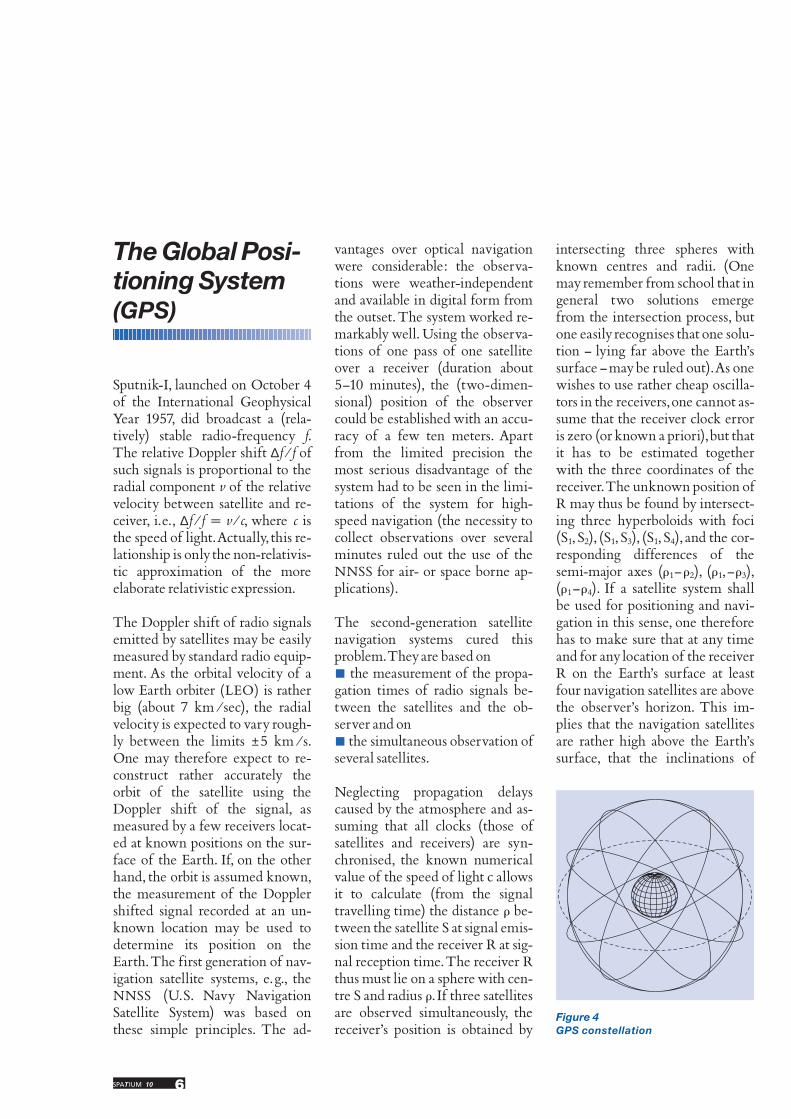
intersecting three spheres withknown centres and radii. (Onemay remember from school that ingeneral two solutions emergefrom the intersection process, butone easily recognises that one solu-tion – lying far above the Earth’ssurface – may be ruled out).As onewishes to use rather cheap oscilla-tors in the receivers, one cannot as-sume that the receiver clock erroris zero (or known a priori), but thatit has to be estimated togetherwith the three coordinates of thereceiver. The unknown position ofR may thus be found by intersect-ing three hyperboloids with foci(S1, S2), (S1, S3), (S1, S4), and the cor-responding differences of thesemi-major axes (�1–�2), (�1, –�3),(�1–�4). If a satellite system shallbe used for positioning and navi-gation in this sense, one thereforehas to make sure that at any timeand for any location of the receiverR on the Earth’s surface at leastfour navigation satellites are abovethe observer’s horizon. This im-plies that the navigation satellitesare rather high above the Earth’ssurface, that the inclinations of

6SPAT IUM 10

Figure 4GPS constellation

their orbital planes w. r. t. to theequatorial plane are rather big, andthat the satellites are well separat-ed (equally spaced) in the orbitalplanes.

The best known of these secondgeneration satellite systems is thefully deployed U.S. Global Posi-tioning System (GPS). Figure 4 il-lustrates the GPS configuration asseen from a latitude of 35° fromoutside the actual configuration.The constellation consists of sixorbital planes, each inclined by 55°w. r. t. the equator and separated by60o in it. The satellite orbits them-selves are almost circular withradii of about 26.500 km – givingrise to revolution periods of half a

sidereal day. There are (at least)four satellites, well separated fromeach other, in each orbital plane.The satellites transmit informa-tion on two L-band wavelengths,L1 and L2, with wavelengths of�1 = 19 cm, �2 = 24 cm. Figure 5shows a GPS satellite. Obviously,the antenna array always has topoint towards the centre of theEarth. The solar panels axes haveto be perpendicular to the lineSun–satellite at any time. The atti-tude emerging from these require-ments is actively maintained usingmomentum wheels within thesatellite’s body.

Alternative systems are the Russ-ian GLONASS (Global Naviga-

tion Satellite System) or the Euro-pean GALILEO system, to be de-ployed by the European SpaceAgency (ESA) in the first decadeof the third millennium. All sys-tems are based on the same princi-ples.

In order to fully appreciate the re-sults presented subsequently wehave to inspect the actual observ-ables of second-generation naviga-tion satellite systems in more de-tail. The signal transmitted bysatellite S at time t S (satellite clockreading) contains this transmis-sion epoch. This information maybe used by the receiver R to com-pute the so-called pseudorange pusing the reading of the receiverclock at signal reception time t R:

p = c ( tR – t S ) 1

In the “best possible of fundamen-tal-astronomical worlds” p wouldjust be equal to the geometric dis-tance �. Because neither the satel-lite nor the receiver clocks are ex-actly synchronised with atomictime, because the signal has totravel through the Earth’s atmos-phere, and because of the measure-ment error the actual relationshipbetween the pseudorange and thedistance � reads as

p = �+c �tR– c �tS +��T +��I (�)+� 2

where � is the distance betweensatellite S and receiver R, �tR thereceiver clock error, �t S the satel-lite clock error, ��T the propaga-tion delay due to the electricallyneutral atmosphere, ��I the delaydue to the ionosphere (caused bythe free electrons in layers be-tween 200 km and 1200 km

7SPAT IUM 10

Figure 5GPS IIR spacecraft (credit USAF).

height), and � the measurementerror. For the code measurementsthe error � is of the order of a fewdecimetres allowing for real timepositioning with about one meteraccuracy. For scientif ic purposesthe phase-derived pseudorange p’is extensively used. The receiver Rgenerates this observation bycounting the incoming carrierwaves (integers plus fraction part)and by multiplying the result bythe speed of light c. This observ-able is related to the geometricaland atmospheric quantities by

p’=�+c �tR–c�tS+��T –��I (�)+N�+�’ 3

Obviously, the code- and phase-derived pseudoranges are inti-mately related. The key differenceresides in the fact that the phase

measurement error �’ is very small,of the order of few millimetres,whereas the code-derived meas-urement error � is about a factor of100 larger. This positive aspect issomewhat counterbalanced by theterm N�, the initial phase ambigu-ity term, which is unfortunatelyunknown. The parameter N,known to be integer, has to be esti-mated as a real-valued parameter.Under special conditions it is pos-sible a posteriori to assign the cor-rect integer number to the esti-mated real-valued unknown. Notethat the ionospheric signal delay inequation 2 is replaced by a phase ad-vance in equation 3.

The term “best possible of funda-mental-astronomical worlds” wascoined to characterise a world, in

which clock corrections and at-mosphere delays do not exist. Thefollowing results will show thatthis label is not really justif iedwhen interested in other than geo-metrical aspects. The clock- andatmosphere-related “nuisance”terms are, as a matter of fact, ex-ploited to synchronise clocksworldwide and to describe theEarth’s atmosphere. The limitedspace allows us only to present oneof these aspects (the derivation ofionosphere models from a world-wide net of GPS receivers). All theother results are related to theterm �, the distance between satel-lite and receiver. The satellite or-bits, the positions (and tectonicmotions) of the observing sites,and the Earth rotation parametersare derived from �.

8SPAT IUM 10

Figure 6The IGS network in March 2003 (credit: IGS Central Bureau; JPL; Pasadena, California.

thti

mcm4

eisl

parc riog

ohigvesl syog maw1 cas1dav1

davr

coyqantc

conz lpgscord

copounsa

sant valpgoug

suth

sirno

sulmrbay

harbhrao

pert nnor cedu

mac1

hob2

ous2chat

auck

noumyarryar2 yar1

alicsumn

sachholm

resoeurk

thu2 alrt

kelyreykreyz

hotn

nya1 nyal

suva

fale

pdl

gmas mas1

bako

coco

irkjirkt

tixi

ulab

galariop

bogtkourkou1

areqiqqe

braz

chpi

cfag

fortasc1

tgcv

ykronklg

msku

mbar

mali

zamb

sey1

kerg

mald

dgar

thu3

qaq1

bahr

kit3

artu nvsk

nril

pol2

kstu

sele

chum

urumguao

hydejiscban2

karr

ntus

lhaskurm

wuhnxian

yaktyakz

khai

mag0

pirno

tnmltwtf

shao

toms

bjfs

bili

petp

yssksuwn

daej

guarn

lae1

darwdarr

jab1

tow2 kouc

kwj1

The InternationalGPS Service (IGS)and the Code AnalysisCentre

The International GPS Service(IGS) was created in 1991. It be-came fully operational, after a pilotphase of about two years, on Janu-ary 1, 1994. The IGS is based on avoluntary collaboration of scien-tif ic and academic organisations inthe fields of geodesy, space science,and fundamental astronomy. Bigresearch organisations like NASA,JPL, ESA, etc. contribute as well asNational Geodetic Survey institu-tions, and universities. The IGSdeployed and maintains a networkof more than 200 globally distrib-uted permanent GPS sites. Figure 6,taken from the IGS homepage,gives an impression of the net-work.

The IGS network ref lects to someextent the fact that the IGS is a vol-untary collaboration: The stationdistribution is far from homoge-neous, but one can also see thatthere are only few “empty” areasleft today. Each IGS station trackseach GPS satellite in view. At leastonce per 30 seconds all availablecode and phase measurements onthe two frequencies are stored –giving rise to 2 x 8640 measure-ment epochs per day. At least on adaily turnaround cycle the rawdata are sent (via internet or tele-phone modems) to regional and

global data centres, from wherethey can be retrieved by the widerscientif ic community, but also(perhaps more importantly) by theIGS Analysis Centres to generatethe IGS products. There are cur-rently seven IGS Analysis Centres(three in the USA, one in Canada,two in Germany (where the one atESA should be considered asmulti-national) and one, calledCODE, situated at the Universityof Bern. CODE is a joint ventureof the University of Bern’s Astro-nomical Institute (AIUB) withthe Swiss Bundesamt für Landes-topographie (Swisstopo), the Ger-man Bundesamt für Kartographie undGeodäsie (BKG) and the French In-stitut Géographique National (IGN).The work of the IGS AnalysisCentres (AC) is truly remarkable.Every day, a table of geocentric or-bital positions is generated by eachof the AC's for each active GPSsatellite with a spacing allowing it

to reconstruct the satellites’ posi-tions and velocities with cm-pre-cision for any time argumentwithin the day. These satellite or-bits originally were the primaryIGS product. They are a big relieffor research and production organ-isations using the GPS for high-ac-curacy surveys. It is, e. g., worthmentioning that since 1991 theSwiss f irst order geodetic survey isuniquely based on GPS and on theIGS products. A similar develop-ment was observed in most othercountries worldwide.

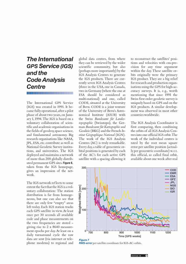
The IGS Analysis Coordinator isf irst comparing, then combiningthe orbits of all IGS Analysis Cen-tres into one official IGS orbit. Thework of the individual centres israted by the root mean squareerror per satellite position (actual-ly per geocentric coordinate) w. r. t.this official, so called final orbit,available about one week after real

9SPAT IUM 10

Figure 7RMS-error per satellite coordinate for IGS-AC-orbits.

300

200

100

0

Wei

ght

ed R

MS

[m

m]

Time [GPS weeks]700 800 900 1000 1100 1200

CODEMR

GFZJPLNGSSIOIGR

ESA

time. Figure7 shows these root meansquare errors for each centre since1994 to March 2003. The consis-tency of the best contributions istoday of the order 2–3 cm. Notwithout pride we note that theCODE-contribution (red curve)always was among the best sincethe advent of the IGS. (Note thatthe green curve labelled “IGR”characterises the combined IGSrapid solution, which is alreadyavailable within one day after “realtime”.) Elementary geometric con-siderations show that this orbit ac-curacy of few cm is sufficient formillimetre precision positioning onthe Earth or in Earth-near space(e. g., for LEO's). It is a remarkableIGS achievement that the GPS or-bits may be considered virtually“error-free” for most applications.

ScientificApplications

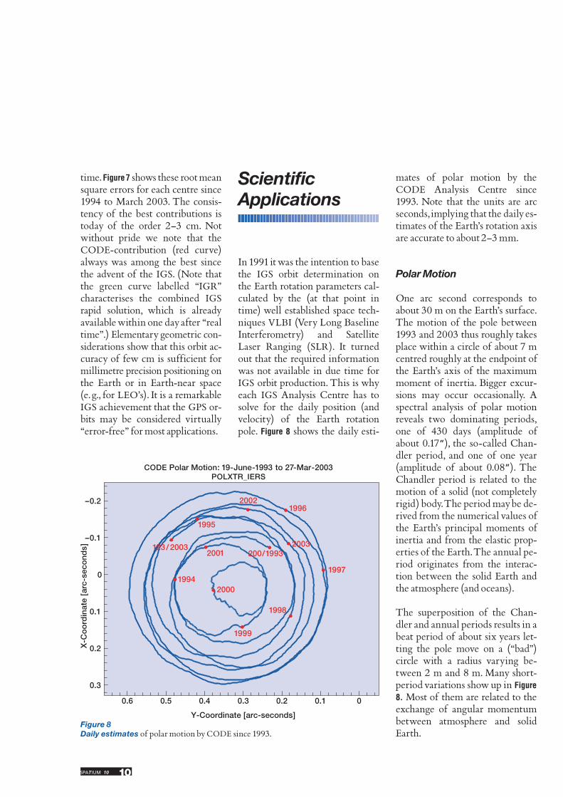
In 1991 it was the intention to basethe IGS orbit determination onthe Earth rotation parameters cal-culated by the (at that point intime) well established space tech-niques VLBI (Very Long BaselineInterferometry) and SatelliteLaser Ranging (SLR). It turnedout that the required informationwas not available in due time forIGS orbit production. This is whyeach IGS Analysis Centre has tosolve for the daily position (andvelocity) of the Earth rotationpole. Figure 8 shows the daily esti-

mates of polar motion by theCODE Analysis Centre since1993. Note that the units are arcseconds, implying that the daily es-timates of the Earth’s rotation axisare accurate to about 2–3 mm.

Polar Motion

One arc second corresponds toabout 30 m on the Earth’s surface.The motion of the pole between1993 and 2003 thus roughly takesplace within a circle of about 7 mcentred roughly at the endpoint ofthe Earth’s axis of the maximummoment of inertia. Bigger excur-sions may occur occasionally. Aspectral analysis of polar motionreveals two dominating periods,one of 430 days (amplitude ofabout 0.17”), the so-called Chan-dler period, and one of one year(amplitude of about 0.08”). TheChandler period is related to themotion of a solid (not completelyrigid) body. The period may be de-rived from the numerical values ofthe Earth’s principal moments ofinertia and from the elastic prop-erties of the Earth. The annual pe-riod originates from the interac-tion between the solid Earth andthe atmosphere (and oceans).

The superposition of the Chan-dler and annual periods results in abeat period of about six years let-ting the pole move on a (“bad”)circle with a radius varying be-tween 2 m and 8 m. Many short-period variations show up in Figure8. Most of them are related to theexchange of angular momentumbetween atmosphere and solidEarth.

10SPAT IUM 10

CODE Polar Motion: 19-June-1993 to 27-Mar-2003POLXTR_IERS

Y-Coordinate [arc-seconds]

X-C

oo

rdin

ate

[arc

-sec

ond

s]

–0.2

–0.1

0

0.1

0.2

0.3

0.6 0.5 0.4 0.3 0.2 0.1 0

1999

20001994

1998

1997

19962002

20032001 200/1993

1995

123/2003

Figure 8Daily estimates of polar motion by CODE since 1993.

Length of Day

In inertial space (i. e., w. r. t. thestars) the Earth rotates once aboutits axis in a sideral day, correspon-ding to about 23 h 56 m of atomictime. Figure 9, emerging from thedaily estimates of the CODE AC,shows that the actual length of dayis “far” from constant. Short peri-od variations (e. g., of two weeks)are easily explained by the tidal de-formation of the Earth due to theMoon (the tidal displacementcauses a varying polar moment ofinertia, which in turn leads to avarying angular velocity of Earthrotation). Observe that the bi-monthly changes in the length ofday (lod) are small (amplitudewell below the millisecond), butthat they are easily detected in this

global analysis. The annual varia-tions with amplitudes of aboutone millisecond are more interest-ing.

The phenomenon is explained bycomparing the polar componentof the solid Earth’s angular mo-mentum (which may be derivedfrom the length of day variations)with the so-called atmosphericangular momentum (which is de-rived from the global meteorologi-cal networks, registering pressure,temperature, and wind profiles).

Figures 10a and 10b compare the rel-ative polar (axial) angular mo-menta of the solid Earth (red line)and of the Earth’s atmosphere.The “true” angular momentum ofthe solid Earth was used in the caseof Figure 10a, whereas a low-orderpolynomial was removed fromthis time series in Figure 10b. The

11SPAT IUM 10

Figure 9Length of day variations 1993–2003.

700 800 900 1000 1100 1200Time [GPS-weeks]

CODE Excess Length of Day: 19-June-1993 to 27-Mar-2003POLXTR_IERS

Exc

ess

Leng

th o

f D

ay [

ms]

3

2

1

0

–1

–0.2

–0.1

0

0.1

0.2

1993 1994 1995 1996 1997 1998 1999 2000 2001 2002 2003

chi_

3

Year

codncep

Figure 10aPolar angular momenta solid Earth and athmosphere.

correlation of the two curves –which are completely independent– is striking in both cases. In Figure10b the correlation coefficient is r = 0.98, implying that the polarcomponent of the system (solidEarth plus atmosphere) is almostperfectly conserved – at least whenconsidering variations with peri-ods of one year or smaller.

Obviously there are variations oflonger period (“decadal” varia-tions) in the polar angular mo-mentum (Figures 10a, 9a), which donot occur in the polar componentof the atmospheric angular mo-mentum. They are undoubtedlyreal. These variations are most in-teresting from the global geody-namics point of view. They may beexplained by the fact that the IGSobserving sites are attached to theEarth’s crust, which is, however,not rigidly attached to the Earth’s

inner shells (in particular to thef luid outer and the rigid inner coreof the Earth). It would be very niceto present pictures correspondingto Figures 10a,b proving the ex-change of angular momentumwith the inner layers, namely man-tle, inner and outer core. Unfortu-nately there are no direct measure-ments of the angular momenta ofthese layers. This may be consid-ered as a disadvantage. On theother hand, one has to acknowl-edge that the study of the decadallod-variations (Figure 9) or of thecorresponding angular momen-tum (red curve in Figure 10a) con-tains very valuable informationconcerning the rotational behav-iour of the Earth’s interior. Geody-namical Earth models must ex-plain the long-term developmentin Figure 10a. With the polar mo-tion time series of Figure 8 it is pos-sible to calculate the other two

components (the equatorial com-ponents) of the solid Earth’s angu-lar momentum and to comparethem with the corresponding at-mospheric quantities, as well. Thecorrelation between the two seriesis rather pronounced, but with cor-relation coefficients around r = 0.7not nearly as high as in the case ofthe polar component.

Plate Motion Velocities

The Chandler period of 430 days(instead of 300 days) clearly indi-cates that the Earth is not rigid.This fact is also supported by Fig-ure 11 showing that the observingsites are not f ixed. The figure isderived from weekly estimates ofthe coordinates of the tracking sta-tions of the IGS network. It turnsout that in the accuracy rangeachieved by the IGS analyses([sub]cm accuracy for the daily es-timates of the coordinates of thetracking sites) it is not possible toassume that the polyhedron of ob-serving sites is rigid. One has totake the relative motion of the sta-tions into account. Figure 11 showsthe “velocity” estimates for thestations processed daily by theCODE analysis centre (from along series solutions). Other space-geodetic techniques are of coursealso capable of determining sta-tion velocities. The unique aspectof GPS analyses is the compara-tively high density of observingsites. The velocities seem small atf irst sight. One is inclined to con-sider velocities of the order of 1–10cm /year as irrelevant. Nothingcould be more wrong: A velocityof 1 cm /year gives rise to a posi-

12SPAT IUM 10

–0.15

–0.1

–0.05

0

0.05

0.1

0.15

1993 1994 1995 1996 1997 1998 1999 2000 2001 2002 2003

chi_

3

Year

codncep

Figure 10bPolar angular momenta solid Earth (trend removed) and athmosphere.

tion change of 1000 km in 100million years! As a matter of fact,these velocities explain the “conti-nental drift” postulated by AlfredLothar Wegener (1880–1930) in1915. At Wegener’s epoch the con-tinental drift, referred to more ap-propriately as plate motion, waspure speculation – today we aremonitoring it in real time.

Electron Density in theAtmosphere

Let us continue our review of thescientif ic exploitation of the GPSby an example related to the at-mosphere, the determination of

the total number of electrons inthe atmosphere. The informationis extracted from the ionosphericrefraction term ��I (�) in equations2, 3. Whereas the results presentedso far were obtained by analysingthe so-called ionosphere-free lin-ear combination of the L1- andL2-observables (which eliminatethe wavelength-dependent ionos-pheric refraction term), the so-called geometry-free linearcombination of the L1- and L2-observations is used for the pur-pose we have in mind now. Thisparticular linear combination ofobservations is the plain differ-ence of the equations of type 2 or 3for the L1- and the L2-wave-

lengths. As all the other terms arewavelength independent, we ob-tain a direct observation of ionos-pheric refraction along the line ofsight between observer and satel-lite by using this difference of ob-servations. The result is propor-tional to the number of electronscontained in a straight cylinder be-tween observer and satellite.Using the phase and code observa-tions from the entire IGS networkone may derive maps of the elec-tron density (the simplest modelassumes that all free electrons arecontained in a layer in a givenheight H – usually set to H = 400km).At CODE, such maps are pro-duced with a time resolution of

13SPAT IUM 10

Figure 11Station velocities estimated by CODE Analysis Center.

ohig

1 cm/year velocity

vesl

maw1

mcmu

cas1dav1

chat

pama

tahi

mkea

kokb

fairwhit yell

will

albhdrao

quingol2

amc2piet1

mdo1monp

churflin

dubosch2

kely

stjowes2

brmu

nlibalgo nrc1

codeusno

aomlrom6

jama

moin

gala

barbcro1

kourbogt

fort

areqbraz

eislcord

lpgs

sant

riog

goug

suth

asc1

harkhrao

ykro

mas1

malisey1

dgar

thu1

reykhofn

nyal

tromtro1

kiru

nya1

tixi

yakz

bili

mago

petryssk

tskbusud

mac1

auck

noum

hob2

darw

tid2cedu

tow2

pertyar1

alickarrcoco

bako

ntus

kwj1guampimo

taiw

lhasxian

wuhn

shao

kstuirkt

urumsell

pol2

kit3taes

daesjuwn

artu

ramo bahr

niconssp

zeck

mategrascagl

noto

onsa

glsvzwenmdvo

mets

ankr

kerg

iisc

pots

casc

wsrthers wtzr

toul

bor1

villmadr

wettkosgbrussjdvzimm

bogopenc

jozelama

upadmedigraz

gope

two hours. Figure 12 shows one ofthese snapshots. The electron den-sity is given in TECU's (TotalElectron Content Units), 1 TECUcorresponding to 1016 electronsper m2.

Several mechanisms are responsi-ble for producing free electrons inthe Earth’s atmosphere. The mostimportant is related to the Sun’sUV radiation ionising the mole-cules in the upper atmosphere.

This is why the “spot” of maxi-mum electron density closely fol-lows the projection of the Sunonto the Earth’s surface (subsolarpoint). The maximum is actuallylagging behind the subsolar pointby about two hours. In Figure 12 wesee a bifurcation of the ionospheredensity along the geomagneticequator (dotted line), an interest-ing aspect due to the Earth’s mag-netic f ield. Internally, the electrondensity is represented by a spher-

ical harmonics series with about250 terms. The zero-order termrepresents the mean electron den-sity. Figure 13 shows the develop-ment of this mean electron densi-ty, which may be inspected as afunction of time.

This is a good example for solar-terrestrial relationships. A spec-trum of the time series underlyingFigure 13 shows that the shortestperiod corresponds to the rotation

14SPAT IUM 10

Figure 12Map of total ionospheric content of electrons (1 TECU =1016 electrons per m3).

Geographic longitude [degrees]

CODE’s rapid ionosphere maps for day 17, 2003 – 10:00 UT

Geo

gra

phi

cal l

atitu

de

[deg

rees

]

60

30

0

–30

–60

–180 –135 –90 –45 0 45 90 135 180

TEC [TECU]

0 10 20 30 40 50 60 70 80

15SPAT IUM 10

period of the Sun (about 27 days),indicating that the UV radiation is related to the sunspots. Anotherprominent period is the annualperiod,which is due to the varyingdistance between Sun and Earth(because of the Earth’s orbitaleccentricity of e = 0.016). Thelongest period corresponds to the11-year sunspot cycle. It should be pointed out that Figure 13 prob-ably represents the best historyof the density of free electrons.Many more figures of this typemight be generated by replacingthe zero order term of the devel-opment of electron densities bythe higher-order coefficients ofthe harmonic series underlyingFigure 12.

Determination of the Earth’sGravity Field: Review andOutlook

It would have been fair and appro-priate to discuss our knowledge ofthe Earth’s gravity field in the in-troductory section together withthe geometrical properties of theEarth. This was not done becauseour knowledge of the global as-pects of the Earth’s gravity fieldwas very poor in the pre-space age:It was of course known that theEarth is, in good approximation, asphere (meaning that the gravityfield is that of a point mass).Thought experiments due to I.Newton and expeditions per-formed in the 18th century then re-

vealed that the next better approx-imation for the shape of the Earthwas that of a spheroid with a f lat-tening of about f=1/300 (giving riseto one second-order term of thegravity field, the so-called “dy-namical f lattening”). (Gravimetermeasurements on the Earth’s sur-face indicated that there were sig-nificant local and regional varia-tions of the Earth’s gravity field,but it was not possible to use thesemeasurements to derive a consis-tent global gravity field of theEarth).

The analysis of the orbits of artif i-cial Earth satellites, starting in the1960s, greatly improved ourknowledge of the Earth’s gravityfield. Instead of only two terms(the mass of the Earth and the dy-namical f lattening) a few thou-sand terms could be determinedwith reasonable accuracy in thefirst era of satellite geodesy. Thetwo Lageos satellites (the acronymstanding for Laser GEOdeticSatellite) were paramount for thistask. The satellites were designedto minimise the impact of non-gravitational forces (the sphere of70 cm diameter consists of Urani-um) on the orbital motion and tooptimise their observation by theLaser technique (Lageos II isshown in Figure 14).

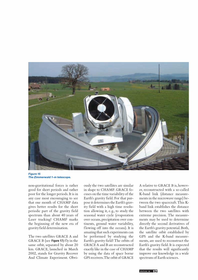
Figure 15 shows University ofBern’s 1 m telescope at Zimmer-wald, which may be used as an op-tical telescope, but also as trans-mission and receiving device forSatellite Laser Ranging (SLR).The Laser technique is used togenerate very short light pulses(few ten picoseconds). The meas-

1995 1996 1997 1998 1999 2000 2001 2002 2003 2004

Time [years]

CODE GIM time series from 01-Jan-1995 to 31-Mar-2003

Mea

n T

EC

[T

EC

U]

60

50

40

30

20

10

Figure 13Mean TEC values 1995–2003.

urement simply is the light travel-ling time of the Laser pulse fromthe observatory to the satellite andback. Due to the divergence of theLaser beam and due to the limitednumber of ref lectors onboard thesatellite (Figure 14) only few re-f lected photons may be detectedin the observatory. The techniquehas outstanding properties: Theaccuracy is high (few picosecondscorresponding to about 1 cm inrange) and the atmospheric effectsmay be modelled with highest ac-curacy (sub-cm) using only stan-dard meteorological measure-ments at the sites. The technique

has, however, also severe disadvan-tages: good weather is a precondi-tion (the clouds in Figure 15 wouldnot allow it to track satellites).Moreover, a Laser observatory israther bulky and expensive, whichis why there exist only about thirtyobservatories today,which are glob-ally coordinated by the Internation-al Laser Ranging Service (ILRS).

The sparseness of the Laser sitesmakes it therefore impossible tocontinuously track the orbit of aparticular satellite. This situationis not at all ideal for the analysis ofsatellite orbits.

This circumstance was one of thekey motivations to look for alter-native space borne methods to de-termine the Earth’s gravity field.All new methods rely on GPS todetermine the orbit of the spacevehicle(s) used to determine theEarth’s gravity field and on theIGS products to model the GPSorbits and clocks. Figure 16 showsan artist’s view of the German re-search satellite CHAMP (ChAl-lenging Minisatellite Payload).Champ was launched in July2000. It is, as the name implies, amultipurpose satellite, allowingatmospheric sounding, and the de-termination of the magnetic andthe gravity fields. The gravity fieldis recovered from analysing thesatellite’s orbits using the GPS.This is possible because the satel-lite carries a space borne GPS re-ceiver ( JPL’s blackjack receiver).CHAMP f lies at rather low alti-tudes (from initially 450 km to300 km at end of the mission in2005). In view of the bulkiness ofthe satellite non-gravitationalforces, residual air drag in particu-lar, do seriously affect the orbit ofthe satellite – and therefore alsothe determination of the Earth’sgravity field. CHAMP copes withthis problem by so-called ac-celerometers, in essence a probemass in the satellite’s interior(shielded against non-gravitation-al forces).The displacement of thisprobe mass in the satellite-fixedreference frame may be used to“determine” the non-gravitationalforces. This is, of course, only pos-sible within certain limits given bythe error spectrum of the ac-celerometers. It turns out that theseparation of gravitational and

Figure 14The Lageos satellite.

16SPAT IUM 10

non-gravitational forces is rathergood for short periods and ratherpoor for the longer periods. It is inany case most encouraging to seethat one month of CHAMP datagives better results for the shortperiodic part of the gravity fieldspectrum than about 40 years ofLaser tracking! CHAMP marksthe beginning of the new era ofgravity field determination.

The two satellites GRACE A andGRACE B (see Figure 17) f ly in thesame orbit, separated by about 20km. GRACE, launched in March2002, stands for Gravity RecoverAnd Climate Experiment. Obvi-

ously the two satellites are similarin shape to CHAMP. GRACE fo-cuses on the time variability of theEarth’s gravity field. For that pur-pose it determines the Earth’s grav-ity field with a high time resolu-tion allowing it, e. g., to study theseasonal water cycle (evaporationover oceans, precipitation over con-tinents, ground water variability,f lowing off into the oceans). It isamazing that such experiments canbe performed by studying theEarth’s gravity field! The orbits ofGRACE A and B are reconstructedexactly like in the case of CHAMPby using the data of space borneGPS receivers.The orbit of GRACE

A relative to GRACE B is, howev-er, reconstructed with a so-calledK-band link (distance measure-ments in the microwave range) be-tween the two spacecraft. This K-band link establishes the distancebetween the two satellites withextreme precision. The measure-ments may be used to determinedirectly the second derivatives ofthe Earth’s gravity potential. Both,the satellite orbit established byGPS and the K-band measure-ments, are used to reconstruct theEarth’s gravity field. It is expectedthat the results will significantlyimprove our knowledge in a widespectrum of Earth sciences.

17SPAT IUM 10

Figure 15The Zimmerwald 1-m telescope.

The third of the new generationsatellites to determine the Earth’sgravity field is ESA’s GOCE satel-lite, shown in Figure 18 (GOCEstanding for Gravity field andsteady-state Ocean Circulation Ex-periment). As the name implies,GOCE is a combined mission tomeasure gravity and Ocean circu-lation. GOCE wants to establishthe mean gravity field of the Earthwith the highest possible accuracyand spatial resolution. When de-termining the gravity field associ-ated with a mass distribution, oneobtains, as a by-product, equipo-tential surfaces. The equipotentialsurface at sea level is called thegeoide. The geoid to be determin-ed by GOCE will be of greatest

importance for the determinationand monitoring of ocean circula-tion. For this purpose it is, in addi-tion,necessary to determine the so-called sea surface topography usingthe measurements of altimetersatellites, reconstructing the sea sur-face using the radar echo tech-nique. The difference between thegeometrically established sea sur-face and the GOCE geoid gives theelevation of the sea surface over thegeoid. Exactly as in the continents,the water in the oceans has to f low“mountains” to “valleys”. It is in-deed fascinating to see that sci-ences which were considered spe-cial disciplines for few experts arenow developing into one multidis-ciplinary topic in Earth sciences.

Unfortunately we could onlytouch a few aspects related to thisnew era of gravity field determi-nation. For more information werefer to the proceedings of theworkshop Earth Gravity Field fromSpace – From Sensors to Earth Sciences,which was hosted by the ISSI inMarch 2002. The workshopbrought together the leading ex-perts in celestial mechanics, geo-desy, Earth sciences, and in instru-ment manufacturing. Theproceedings of the workshop un-derline the tremendous impact ofthis new sequence of space mis-sions on a very broad field of sci-ence.

18SPAT IUM 10

Figure 16The CHAMP spacecraft launched in July 2000 (credit Astrium).

Summary

Navigation and fundamental as-tronomy are intimately relatedsince hundreds of years. Untilabout thirty years ago global navi-gation relied on measuring angles.Scientif ic discoveries include thephenomena of precession, nuta-tion, secular deceleration of Earthrotation, and polar motion.

With the advent of the space agethe astrometric observation ofstars and planets was replaced bythe measurement of distances (ordistance differences) between ob-servers and artif icial satellites. Asweather-and daytime-independ-ence is an important aspect of nav-igation, the observation tech-niques were moreover movedfrom the optical to the microwaveband of the electromagnetic spec-

trum. In view of the fact that the“old” methods were used for cen-turies, one can truly speak of a rev-olution in navigation, geodesy, andfundamental astronomy.

The scientif ic aspects emergingfrom the new navigation systemsare co-ordinated by the Interna-tional GPS Service (IGS). Polarmotion, length of day, plate tecton-ics, and the Earth’s ionosphere aremonitored with unprecedented ac-curacy. The IGS products are alsoparamount for the success of grav-ity field determination with thenew generation of gravity mis-sions. The new era of gravity fielddetermination will lead to a unifi-cation of geometric and gravita-tional aspects, truly bringing to-gether the three pillars of moderngeodesy and fundamental astrono-my, namely (1) positioning andnavigation, (2) Earth rotation, (3)gravity field determination.

19SPAT IUM 8

Figure 18The GOCE spacecraft to be launched in 2006 (credit: ESA).

Figure 17The pair of GRACE spacecraft launched in March 2002 (credit NASA).

The author

Later on, he held positions as re-search associate from 1983 until1984 at the University of NewBrunswick, Fredericton, Canadaand from 1984 until 1991 at theUniversity of Berne. During thelatter period he was engaged inthe development of the BerneseGlobal Positioning System Soft-ware, which is used today at about150 research institutions world-wide. In 1991 he was elected Pro-fessor of Astronomy and Directorof the Astronomical Institute ofthe University of Berne. His lec-tures cover such fields as celestialmechanics, Earth rotation, stellardynamics and statistics, parameterestimation theory and digital f il-tering theory.

The main research interests ofGerhard Beutler are devoted tofundamental astronomy, celestialmechanics, global geodynamicsand satellite-based positioningund navigation. He is a member of numerous national and inter-national committees and workinggroups, as for example the Schwei-zerische Geodätische Kommis-sion, the American GeophysicalUnion and the European SpaceAgency’s Scientif ic AdvisoryBoard on the European Naviga-tion Satellite System Galileo. As of July 2003 he will serve as Pre-sident of the International Asso-ciation of Geodesy (IGS).

Based on his initiative the CODEProcessing Centre of the Interna-tional Geodetic Society was creat-ed. CODE today is a joint ventureof the Astronomical Institute ofthe University of Berne, the SwissFederal Office of Topography, theInstitute for Applied Geodesy inGermany, and the Institut Géo-graphique National in France.

Gerhard Beutler is a fervent sup-porter of the planned Europeannavigation and positioning systemGalileo, not only because this sys-tem would make more satellitesavailable but also because its dif-ferent orbit characteristics as com-pared to the US GPS system wouldprovide the scientif ic user with anincreased potential of positioningaccuracy.

Gerhard Beutler lives with hisfamily in Schüpfen in the CantonBerne. In his free time he likesbiking through the wonderfullandscapes of the Canton Berne, aswell as playing tennis. Not with-out pride he counts himself to theworld top league of the celestialmechanics tennis players.

Gerhard Beutler was borne inKirchberg in the Canton Berne in1946,where he visited the elemen-tary school. After receipt of thetype C maturity in 1964 he en-rolled at the University of Bernein astronomy, physics and mathe-matics. These subjects turned outto be the ideal theoretical founda-tion when it came to exploring thescientif ic potential of navigationsatellites when the U. S. GlobalPositioning System became opera-tional.

In 1976 G. Beutler received thePh.D. degree with a thesis on Inte-gral Evaluation of Satellite Obser-vations. The second thesis was de-voted to the Solution of ParameterEstimation Problems in CelestialMechanics and Satellite Geodesy.