Satellite-derived Groundwater Storage Estimates and Opportunities for Expanding Research in Arid

Environments NASA Ames DEVELOP Program | Summer 2011

Amber Kuss, San Francisco State University William Brandt, California State University, Monterey Bay

Joshua Randall, Arizona State University Bridget Floyd, University of California, Berkeley

Abdelwahab Bourai, Cupertino High School Michelle Newcomer, San Francisco State University

Cindy Schmidt, Mentor Dr. J.W. Skiles, Mentor

• 9-10 week summer internship • Paid • Using NASA data to solve real world problems • Student-run student-led

2011 Summer Interns

Groundwater level measurements in West Sacramento

Diana Delgado at the NASA Ames Science Symposium

NASA Applied Sciences’ DEVELOP National Program

"Training the next generation of Earth Explorers"

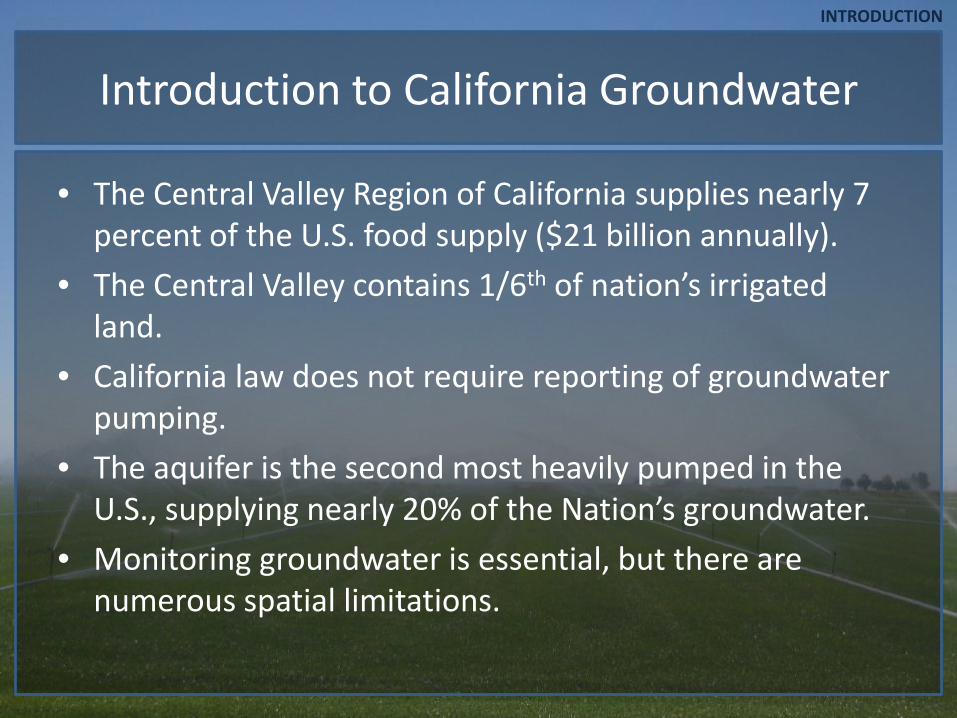
Introduction to California Groundwater

• The Central Valley Region of California supplies nearly 7 percent of the U.S. food supply ($21 billion annually).

• The Central Valley contains 1/6th of nation’s irrigated land.

• California law does not require reporting of groundwater pumping.

• The aquifer is the second most heavily pumped in the U.S., supplying nearly 20% of the Nation’s groundwater.

• Monitoring groundwater is essential, but there are numerous spatial limitations.

INTRODUCTION

Study Area INTRODUCTION

-Two regions where GRACE data is obtained: The Sacramento Hydrologic Region (blue) and the San Joaquin Hydrologic Region (red). -While not the regions and the aquifer are not the same size, the majority of change occurs in the Central Valley aquifer.

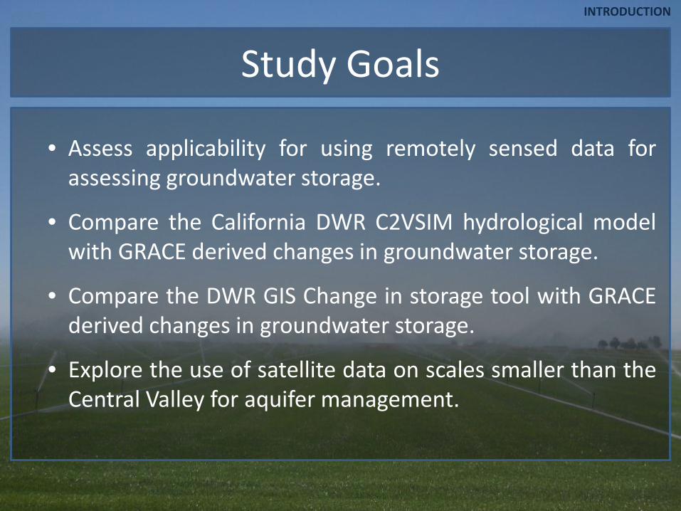
Study Goals

• Assess applicability for using remotely sensed data for assessing groundwater storage.

• Compare the California DWR C2VSIM hydrological model with GRACE derived changes in groundwater storage.

• Compare the DWR GIS Change in storage tool with GRACE derived changes in groundwater storage.

• Explore the use of satellite data on scales smaller than the Central Valley for aquifer management.

INTRODUCTION

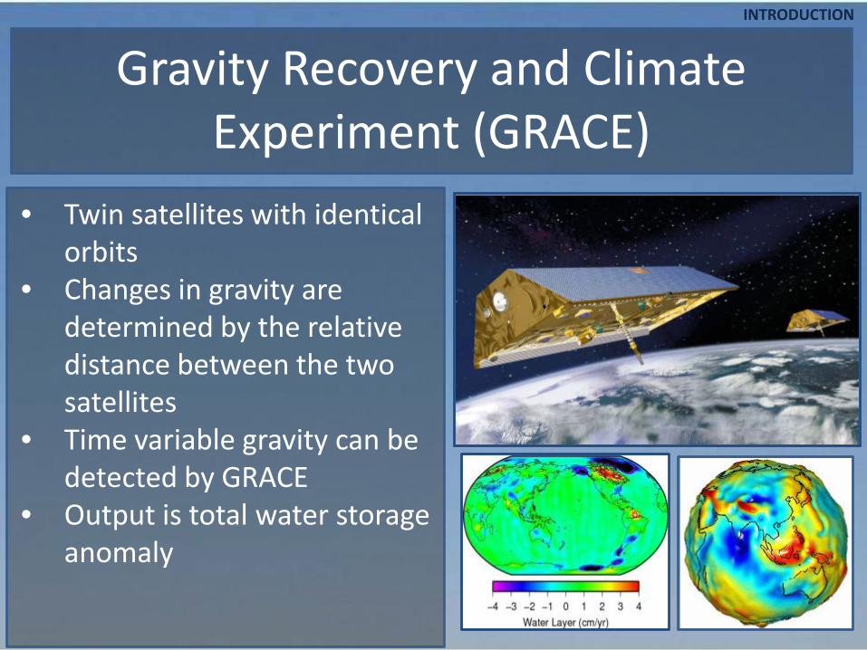
Gravity Recovery and Climate Experiment (GRACE)

• Twin satellites with identical orbits

• Changes in gravity are determined by the relative distance between the two satellites

• Time variable gravity can be detected by GRACE

• Output is total water storage anomaly

INTRODUCTION

What is a gravity anomaly?

(University of Texas Austin, 2011)

The standard of Earth’s gravity anomalies: -mountains = higher gravity -deltas = lower gravity

Time-variable gravity anomalies converted into equivalent units of height in mm. Provides explanation for short term changes on earth like variations in water or ice.

INTRODUCTION

Smoothing Radii

1000 km 300 km 100 km

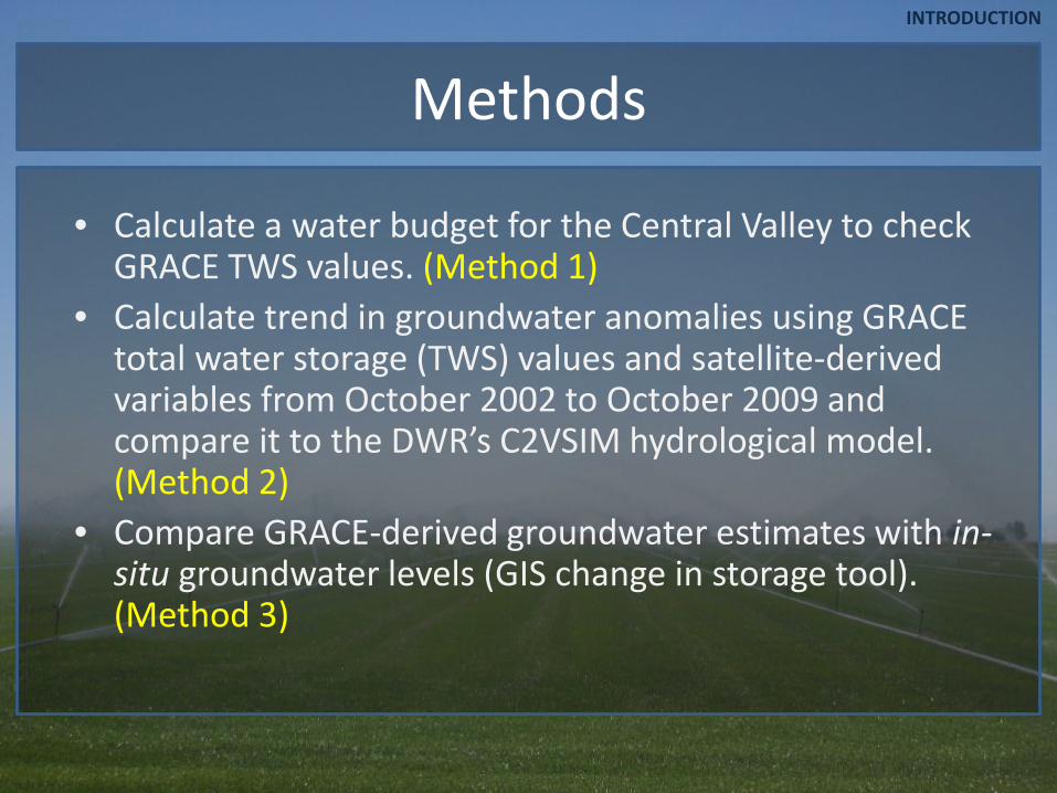
Methods

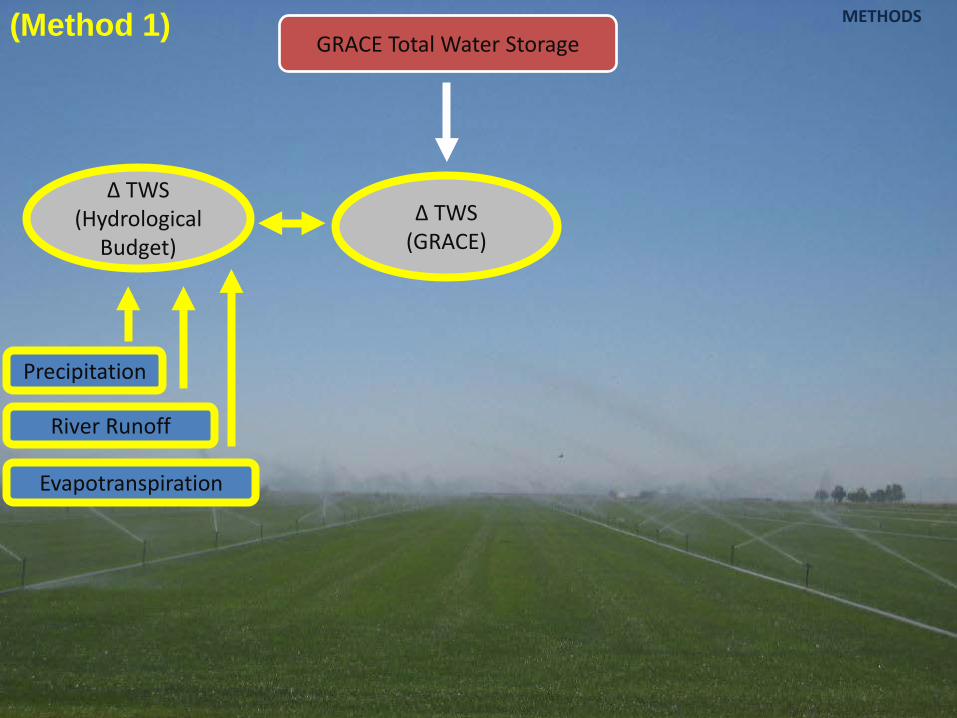
• Calculate a water budget for the Central Valley to check GRACE TWS values. (Method 1)

• Calculate trend in groundwater anomalies using GRACE total water storage (TWS) values and satellite-derived variables from October 2002 to October 2009 and compare it to the DWR’s C2VSIM hydrological model. (Method 2)

• Compare GRACE-derived groundwater estimates with in-situ groundwater levels (GIS change in storage tool). (Method 3)

INTRODUCTION

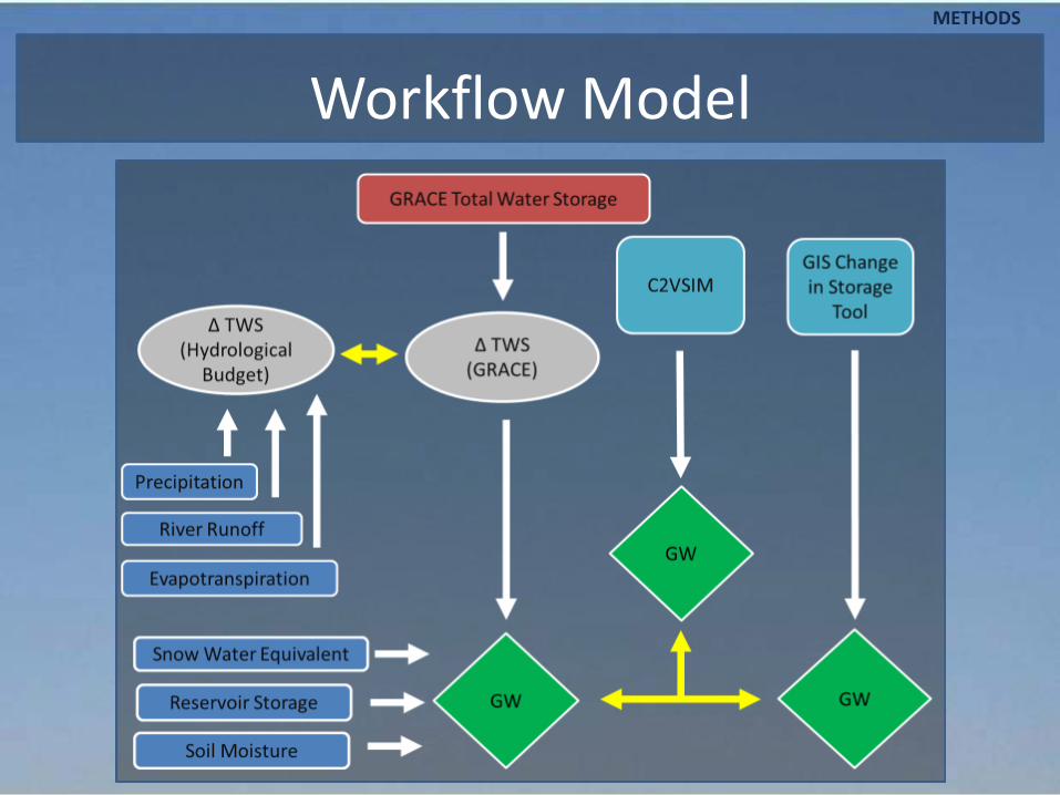
Workflow Model METHODS

Δ TWS (GRACE)

GRACE Total Water Storage METHODS (Method 1)

• The TWS anomalies are variations

in the hydrological budget over a region.

• 84 months (7 yrs) of GRACE data

were obtained. • Smoothing radius of 300 km

• Data obtained from a TRIP Basin

model for both the Sacramento and San Joaquin River Basins and applied in GIS.

Δ TWS (GRACE) METHODS

San Joaquin River Basin Gaussin Halfwidth: 300.000 km Time Anomaly Measurement Error (mm) 111.00 75.87 34.10 130.00 104.14 26.42 228.00 -60.52 21.75 258.50 -31.61 29.87 289.00 -112.33 20.98

Sacramento

San Joaquin

Δ TWS (GRACE) METHODS

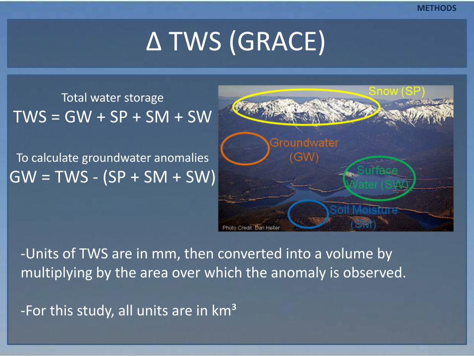
Total water storage TWS = GW + SP + SM + SW

To calculate groundwater anomalies

GW = TWS - (SP + SM + SW)

-Units of TWS are in mm, then converted into a volume by multiplying by the area over which the anomaly is observed. -For this study, all units are in km³

Precipitation

Evapotranspiration

River Runoff

Δ TWS (GRACE)

Δ TWS (Hydrological

Budget)

GRACE Total Water Storage METHODS (Method 1)

ΔTWS = P – (ET + Q)

Evapotranspiration

Precipitation

•MODIS Sensor on the Satellite Aqua

•University of Montana

•PRISM from Oregon State University

•Based on models and real observations

River Runoff/Discharge •Real time daily mean discharge data

•U.S. Geological Survey (USGS)

METHODS

(Method 1)

Comparison of ΔTWS METHODS

Calculation of significance at a = 0.05 level

BudgetGRACE TWSTWS ∆∆ ↔,α

Precipitation

Evapotranspiration

River Runoff

Δ TWS (GRACE)

Snow Water Equivalent

Reservoir Storage

Soil Moisture

Δ TWS (Hydrological

Budget)

GRACE Total Water Storage

GW

METHODS (Method 2)

Calculating GW Anomaly Trends

METHODS

(Method 2)

Soil Moisture

Surface Water Storage

Snow Pack

METHODS

Surface Water Variables

•California Data Exchange Center (CDEC)

•20 largest reservoirs in study area

•The Advanced Microwave Scanning Radiometer for EOS (AMSR-E) • Algorithm converts surface reflectance into soil moisture •The value for each pixel is applied to an average depth of 15 meters

•Snow Data Assimilation System (SNODAS) operated by the National Oceanic and Atmospheric Administration (NOAA)

•Calculates snow water equivalent (SWE)

( ) ( ) ( ) ( )2222SPSMSWTWGW SSSSS +++=

Propagation of Uncertainty Rule

GRACE TW storage data: 2 Types of Error 1. Measurement Error 2. Leakage Error

Error for each hydrological variable is assumed to be 15%

• Statistical Method to determine appropriate amount of uncertainty to be applied to groundwater calculations

METHODS

Error varies depending on the smoothing radius

Anomaly Trends -Seasonal trends in all variables -SW, SM, and SP display fairly steady levels (slight or no decline) while TWS shows decreasing trend after 2006

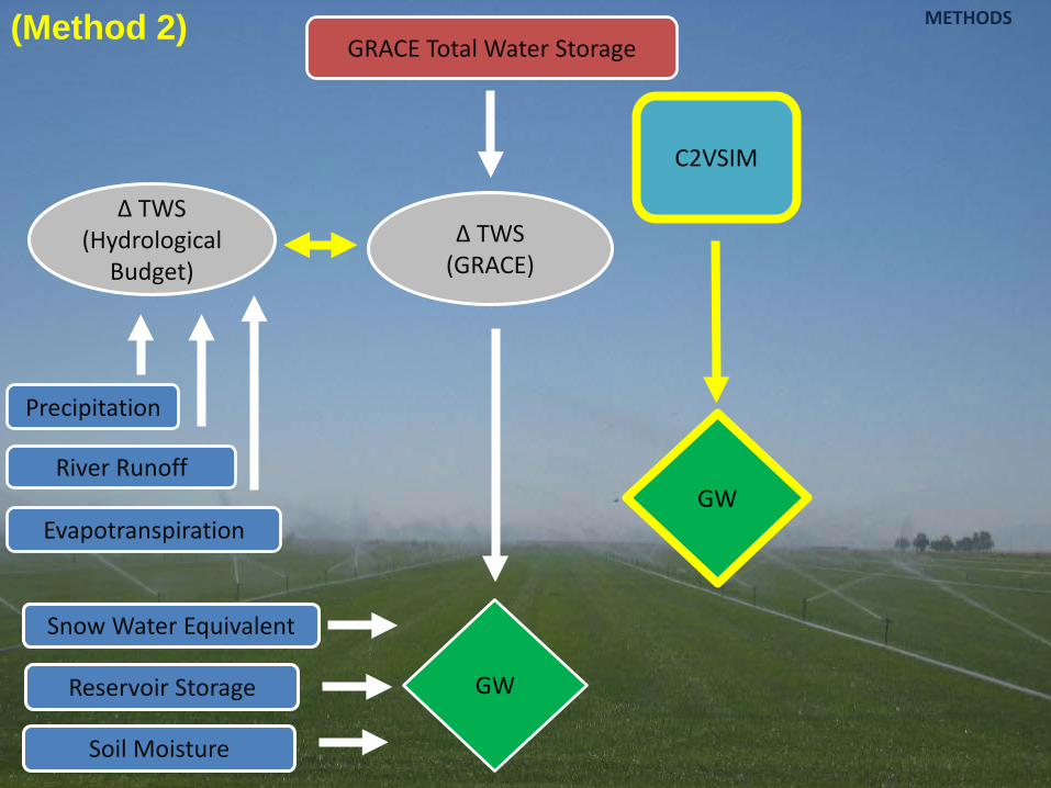
C2VSIM

Precipitation

Evapotranspiration

River Runoff

Δ TWS (GRACE)

Snow Water Equivalent

Reservoir Storage

Soil Moisture

Δ TWS (Hydrological

Budget)

GRACE Total Water Storage

GW

GW

METHODS (Method 2)

C2VSIM Groundwater • A finite-element hydrological

model built to estimate water storage in the Central Valley aquifer

• Model parameters (not limited to):

• P, Q, ET, subsidence, beginning and ending GW for each month

• Calculated anomalies for the data set

• A trend equation was fitted from these anomalies, which was used to find a total volume

METHODS

(Method 2)

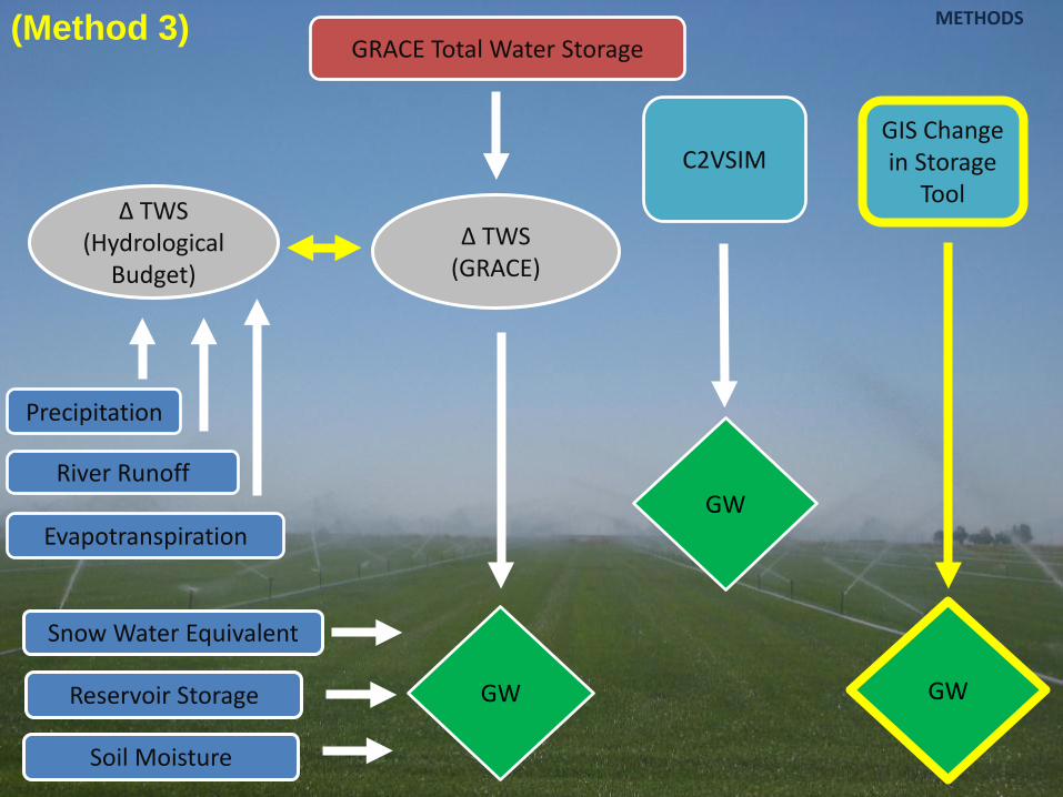
GIS Change in Storage

Tool C2VSIM

Precipitation

Evapotranspiration

River Runoff

Δ TWS (GRACE)

Snow Water Equivalent

Reservoir Storage

Soil Moisture

Δ TWS (Hydrological

Budget)

GRACE Total Water Storage

GW GW

GW

METHODS (Method 3)

Δ GW: GIS Change in Storage Tool

• The GIS change in storage tool was developed by the DWR • The tool interpolates the water levels of wells into TIN layers • Can be used to find change in depths and change in volume over

the Central Valley • Storage coefficient of 0.07 is used (based on a mixture of

unconfined and confined aquifer) • Comparisons are made on a yearly basis (spring to spring)

METHODS

(Method 3)

GIS Change in Storage

Tool C2VSIM

Precipitation

Evapotranspiration

River Runoff

Δ TWS (GRACE)

Snow Water Equivalent

Reservoir Storage

Soil Moisture

Δ TWS (Hydrological

Budget)

GRACE Total Water Storage

GW GW

GW

METHODS

Comparison of GW Storage Trends RESULTS

Comparison of GW Storage RESULTS

- Groundwater estimates for 300 km smoothing radius

- 300 km chosen based on study area and acceptable amount of error in GRACE estimates

- Although estimates from GRACE and C2VSIM are comparable for Central Valley, estimates are not similar for smaller basins

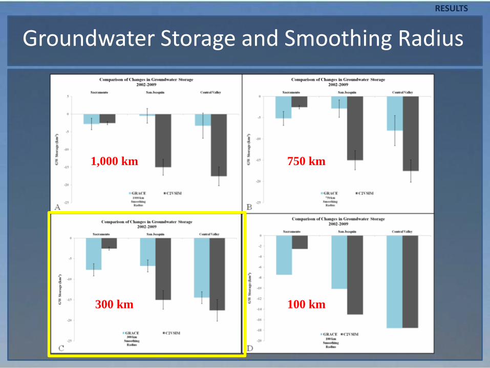
Groundwater Storage and Smoothing Radius RESULTS

1,000 km 750 km

300 km 100 km

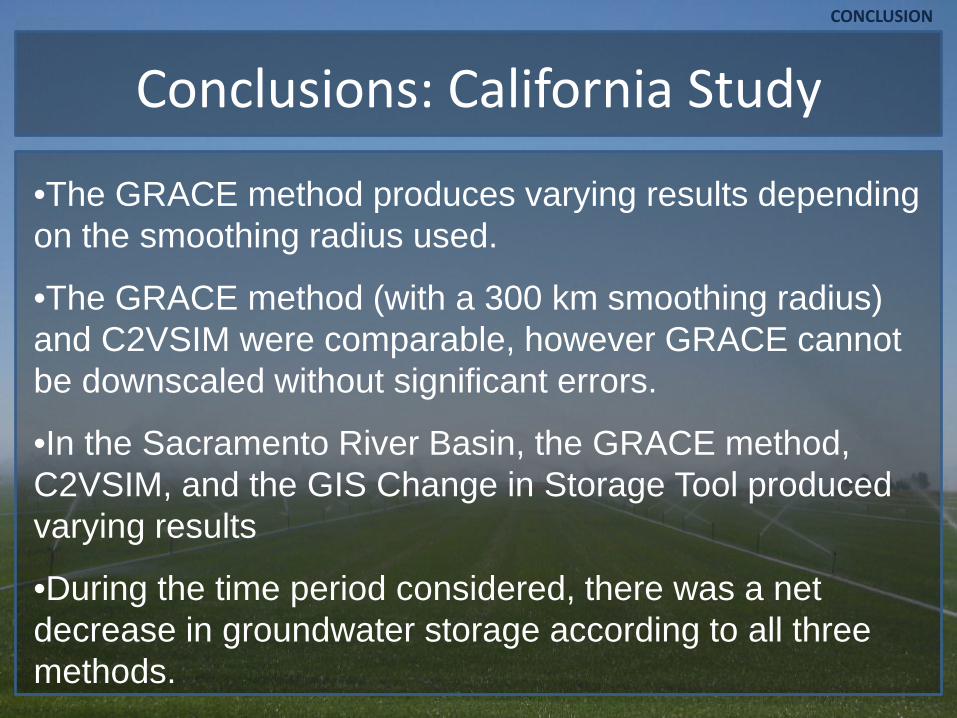
Conclusions: California Study

•The GRACE method produces varying results depending on the smoothing radius used.

•The GRACE method (with a 300 km smoothing radius) and C2VSIM were comparable, however GRACE cannot be downscaled without significant errors.

•In the Sacramento River Basin, the GRACE method, C2VSIM, and the GIS Change in Storage Tool produced varying results

•During the time period considered, there was a net decrease in groundwater storage according to all three methods.

CONCLUSION

GRACE Data Throughout the World Amazon River Basin

Northwestern India

(Rodell et al., 2009)

Obtaining GRACE Data 1. TRIP-defined Basins

2. GRACE Tellus

2 Methods for Obtaining GRACE data: 1. Download specified monthly

values for each basin (TRIP)

2. Download monthly values for the world and then cut and smooth data to specific region (GRACE Tellus)

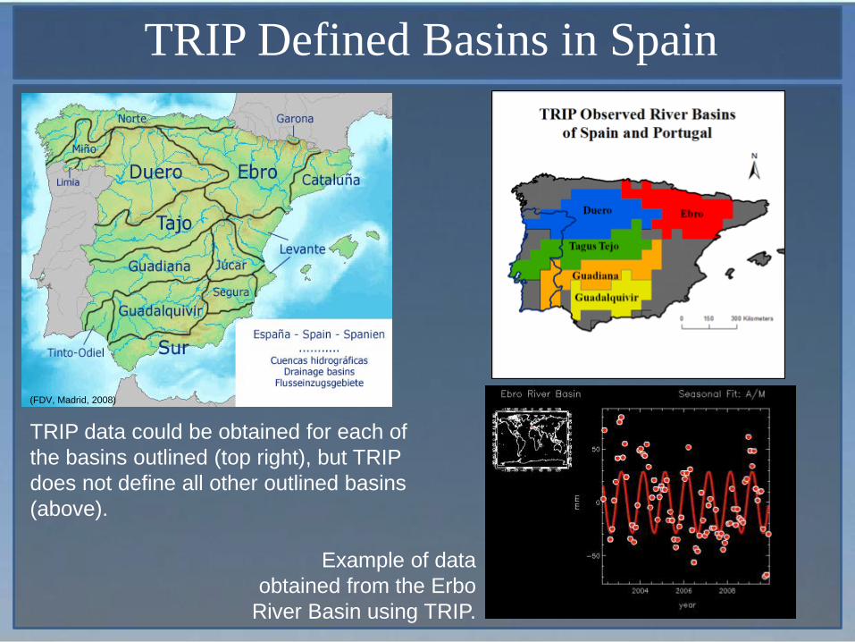
• TRIP could be used for Spain, but not for Saudi Arabia

• GRACE Tellus could be used for both, but involves significantly more processing

(FDV, Madrid, 2008)

TRIP Defined Basins in Spain

TRIP data could be obtained for each of the basins outlined (top right), but TRIP does not define all other outlined basins (above).

Example of data obtained from the Erbo

River Basin using TRIP.

GRACE Tellus Data in Saudi Arabia

GRACE Tellus Processing Requirements •The 1 degree pixels (shown here) needs to be smoothed to reduce the error •Additional processing must be performed

Required Data

Necessary:

• Total Water Storage (TWS) – Satellite • Reservoir Storage (SW) – Country Specific Data • Soil Moisture (SM) – Satellite • Snow Water Equivalent (SP) – Country Specific Data

Helpful to validate GRACE data : Δ TWS = P – (ET + Q)

• Precipitation (P) – Country Specific Data • Evapotranspiration (ET) – Satellite • River Discharge (Q) – Country Specific Data

Next Steps Obtain and process GRACE data

Obtain and process additional variables data

Compare data with existing hydrological models or well data from specific region

Any additional data that may be useful or aid in the development of future projects such as geologic characteristics, pumping and groundwater data for agriculture, industrial, or domestic usage.

Thank You! Thank you to our partner Thank you to everyone else

who helped with this project

CONCLUSION

Thank you to everyone who made this meeting possible.