Embed Size (px)
Citation preview
Satellite data assimilation at NCEPJohn C. Derber
Environmental Modeling CenterNCEP/NWS/NOAA
With contributions from:
P. Van DelstX. Li
M. Kazumori (JMA)K. Okamoto (JMA)
L. CucurullM. Pondeca
R. TreadonW.-S. Wu
D. KleistD. Parrish
Data Assimilation Context
• Data assimilation attempts to bring together all available information to make the best possible estimate of:– The atmospheric state– The initial conditions to a model which will
produce the best forecast.
Data Assimilation Context
• Information sources– Observations– Background (forecast)– Dynamics (e.g., balances between variables)– Physical constraints (e.g., q > 0)– Statistics– Climatology
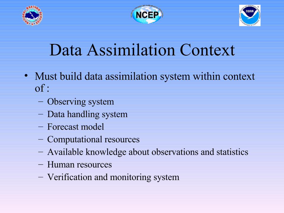
Data Assimilation Context• Must build data assimilation system within context
of :– Observing system– Data handling system– Forecast model– Computational resources– Available knowledge about observations and statistics– Human resources– Verification and monitoring system
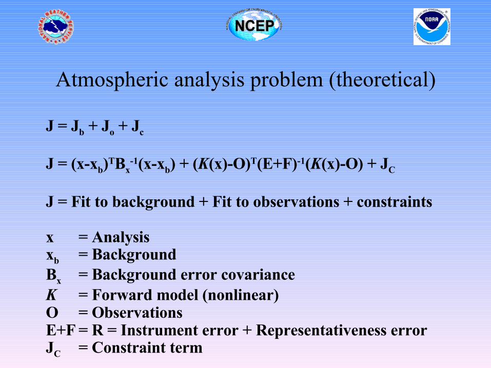
Atmospheric analysis problem (theoretical)
J = Jb + Jo + Jc
J = (x-xb)TBx-1(x-xb) + (K(x)-O)T(E+F)-1(K(x)-O) + JC
J = Fit to background + Fit to observations + constraints
x = Analysisxb = BackgroundBx = Background error covarianceK = Forward model (nonlinear)O = ObservationsE+F = R = Instrument error + Representativeness errorJC = Constraint term
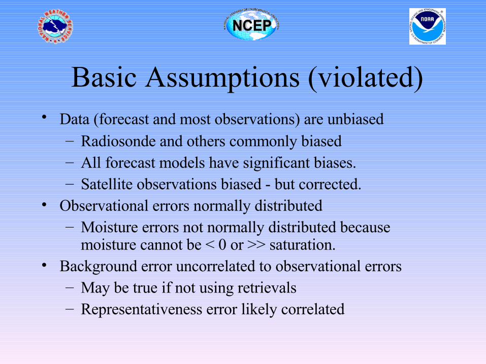
Basic Assumptions (violated)• Data (forecast and most observations) are unbiased
– Radiosonde and others commonly biased– All forecast models have significant biases.– Satellite observations biased - but corrected.
• Observational errors normally distributed– Moisture errors not normally distributed because
moisture cannot be < 0 or >> saturation.• Background error uncorrelated to observational errors
– May be true if not using retrievals– Representativeness error likely correlated
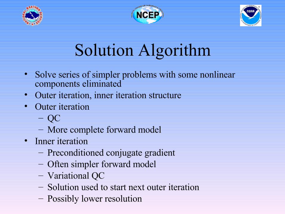
Solution Algorithm• Solve series of simpler problems with some nonlinear
components eliminated• Outer iteration, inner iteration structure• Outer iteration
– QC– More complete forward model
• Inner iteration– Preconditioned conjugate gradient– Often simpler forward model– Variational QC– Solution used to start next outer iteration– Possibly lower resolution
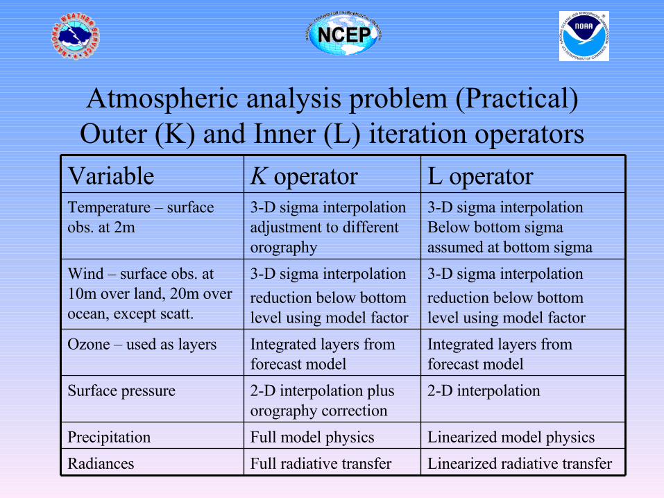
Atmospheric analysis problem (Practical)Outer (K) and Inner (L) iteration operators
Linearized radiative transferFull radiative transferRadiances
Linearized model physicsFull model physicsPrecipitation
2-D interpolation2-D interpolation plus orography correction
Surface pressure
Integrated layers from forecast model
Integrated layers from forecast model
Ozone – used as layers
3-D sigma interpolation
reduction below bottom level using model factor
3-D sigma interpolation
reduction below bottom level using model factor
Wind – surface obs. at 10m over land, 20m over ocean, except scatt.
3-D sigma interpolation Below bottom sigma assumed at bottom sigma
3-D sigma interpolation adjustment to different orography
Temperature – surface obs. at 2m
L operatorK operatorVariable
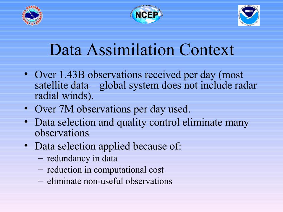
Data Assimilation Context• Over 1.43B observations received per day (most
satellite data – global system does not include radar radial winds).
• Over 7M observations per day used.• Data selection and quality control eliminate many
observations• Data selection applied because of:
– redundancy in data– reduction in computational cost– eliminate non-useful observations
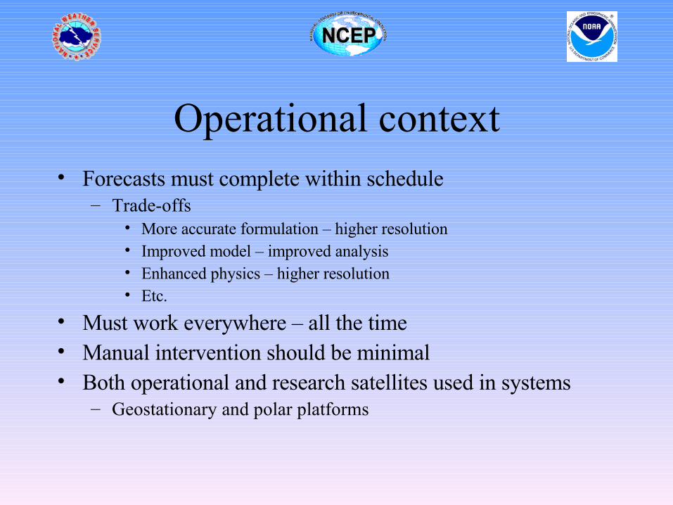
Operational context• Forecasts must complete within schedule
– Trade-offs• More accurate formulation – higher resolution• Improved model – improved analysis• Enhanced physics – higher resolution• Etc.
• Must work everywhere – all the time• Manual intervention should be minimal• Both operational and research satellites used in systems
– Geostationary and polar platforms
Satellite data
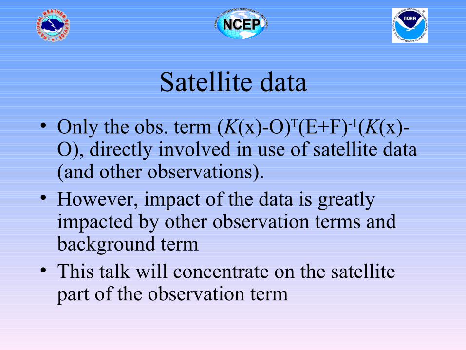
• Only the obs. term (K(x)-O)T(E+F)-1(K(x)-O), directly involved in use of satellite data (and other observations).
• However, impact of the data is greatly impacted by other observation terms and background term
• This talk will concentrate on the satellite part of the observation term
Satellite data context• One of the biggest data assimilation developments
in the last 15 years was allowing the observations to be different from the analysis variables – In variational schemes this is done through the K
operator– In OI, the same thing could be done – but was only
rarely done.– The development allows us to use the observations as
they were observed AND allows the use of analysis variables with nice properties.
Satellite data• Satellite data differ from many conventional data in
that the observations are often indirect observations of meteorological parameters– If x is the vector of meteorological parameters we are
interested in and – y is the observation,– then y = K(x,z),
• where z represents other parameters on which the observations is dependent
• K is the physical relationship between x, z and y
Satellite data
• Example – – y are radiance observations, – x are profiles of temperature, moisture and ozone. – K is the radiative transfer equation and – z are unknown parameters such as the surface emissivity
(dependent on soil type, soil moisture, etc.), CO2 profile, methane profile, etc.
• In general, K is not invertable – thus retrievals.– Physical retrievals – usually very similar to 1D
variational problems (with different background fields)– Statistical retrievals – given y predict x using regression
Satellite data context
• 3-4 D variational analysis can be thought of as a generalization of “physical retrieval” to include all types of data and spatial and temporal variability.
• To use data in 2 steps – retrieval and then analysis-- can be done consistently if K is linear and if one is very careful – but is generally suboptimal.
Satellite data context• Key to using data is to have good characterization
of K – forward model. • If unknowns in K(x,z) – either in formulation of K
or in unknown variables (z) are too large data cannot be reliably used and must be removed in quality control. – example, currently we do not use radiances containing
cloud signal
• Note that errors in formulation or unknown variables generally produce correlated errors. This is a significant source of difficulty.
Satellite data context
• Additional advantages of using observations directly in analysis system– easier definition of observation errors– improved quality control – less introduction of auxiliary information – improved data monitoring
Satellite data assimilation• Satellite observations currently used
– Atmospheric wind vectors• Geostationary• MODIS, TERRA
– SSM/I surface wind speeds– Scatterometers– GPS radio-occultation– SSM/I and TRMM precip. estimates– SBUV ozone profiles– Radiances
Satellite data assimilation
• Satellite observations– Radiances
• AMSU-A (N-15,16,18,METOP,EOS-AQUA)• AMSU-B/MHS(N-15,16,17,18,METOP)• HIRS(N-16,17,18,METOP)• AIRS(EOS-AQUA)• SSM/I – SSM/IS• GOES Sounder (1x1- 4 detectors, G-11, G-12)• Imagers (AVHRR,GOES, METEOSAT, etc.)
Satellite data requirements• Requirements for operational use of observations
– Available in real time in acceptable format– Data files need to contain all necessary information– Assurance of stable data source – Accurate forward model (and adjoint) available– Quality control procedures defined (conservative)– Observational errors defined (and bias removed if
necessary) – Integration into data monitoring– Evaluation and testing to ensure neutral/positive impact
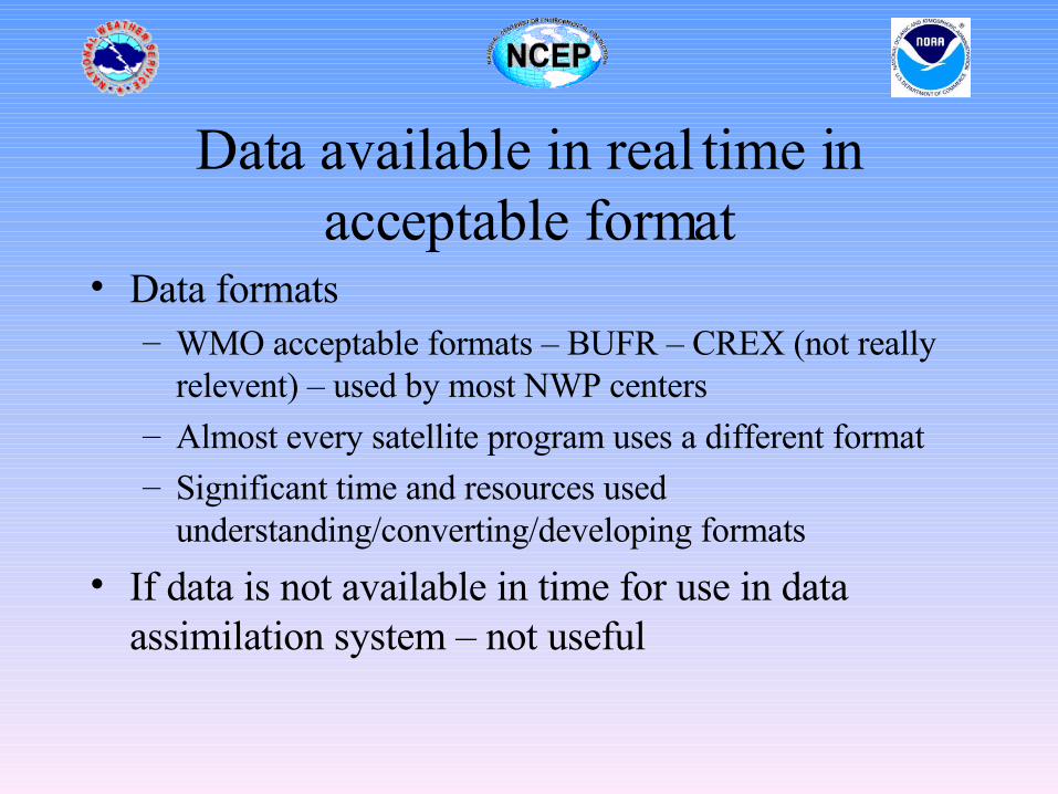
Data available in real time in acceptable format
• Data formats– WMO acceptable formats – BUFR – CREX (not really
relevent) – used by most NWP centers– Almost every satellite program uses a different format– Significant time and resources used
understanding/converting/developing formats
• If data is not available in time for use in data assimilation system – not useful
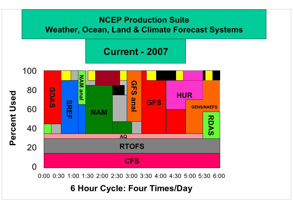
NCEP Production SuiteWeather, Ocean & Climate Forecast Systems
Version 3.0 April 9, 2004
0
20
40
60
80
100
0:00 0:30 1:00 1:30 2:00 2:30 3:00 3:30 4:00 4:30 5:00 5:30 6:00
6 Hour Cycle: Four Times/Day
Pe
rce
nt
Us
ed
RUCFIREWXWAVESHUR/HRWGFSfcstGFSanalGFSensETAfcstETAanalSREFAir QualityOCEANMonthlySeasonal
GD
AS
GF
S an
al
NA
M an
al
CFS
RTOFS
SR
EF NAM
AQ
GFSHUR
RD
AS
Current (2007)
GENS/NAEFS
Current - 2007
NCEP Production SuiteWeather, Ocean, Land & Climate Forecast Systems
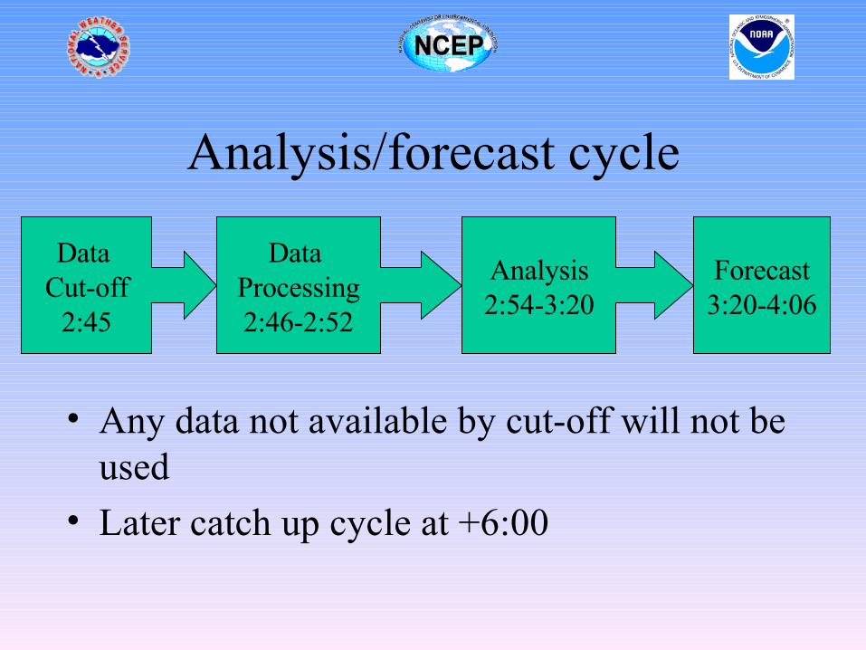
Analysis/forecast cycle
• Any data not available by cut-off will not be used
• Later catch up cycle at +6:00
Data Cut-off
2:45
Data Processing2:46-2:52
Analysis2:54-3:20
Forecast3:20-4:06
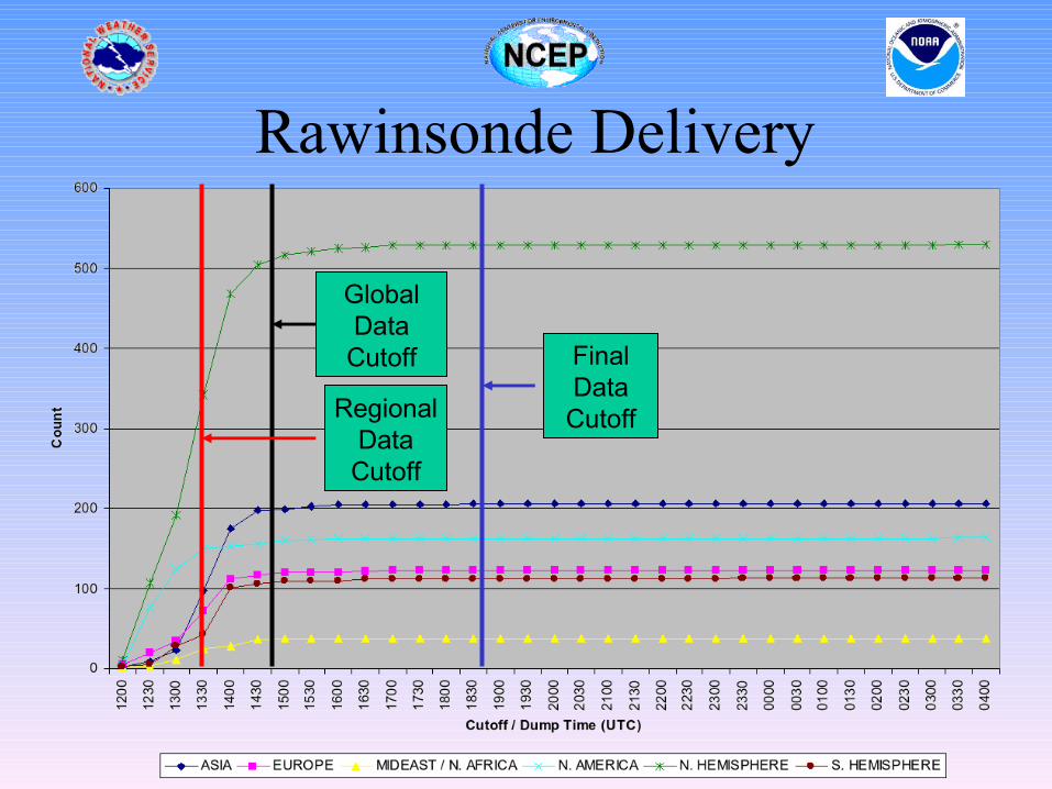
Rawinsonde Delivery
GlobalData
Cutoff
RegionalData
Cutoff
FinalData
Cutoff
POES Data Delivery00Z Average 1B Data Counts
0
0.5
1
1.5
2
0.00 1.00 2.00 3.00 4.00 5.00 6.00 7.00 8.00 9.00 10.00
(Mil
lion
s)
Dump Time - Cycle Time (Hours)
Ave
rag
e R
epo
rt C
ou
nt
HIRS-2 (1bhrs2) HIRS-3 (1bhrs3) AMSU-A (1bamua) AMSU-B (1bamub) MSU (1bmsu)
Loca
tions
Rec
eive
d (M
)
GlobalData
Cutoff
RegionalData
Cutoff
FinalData
Cutoff
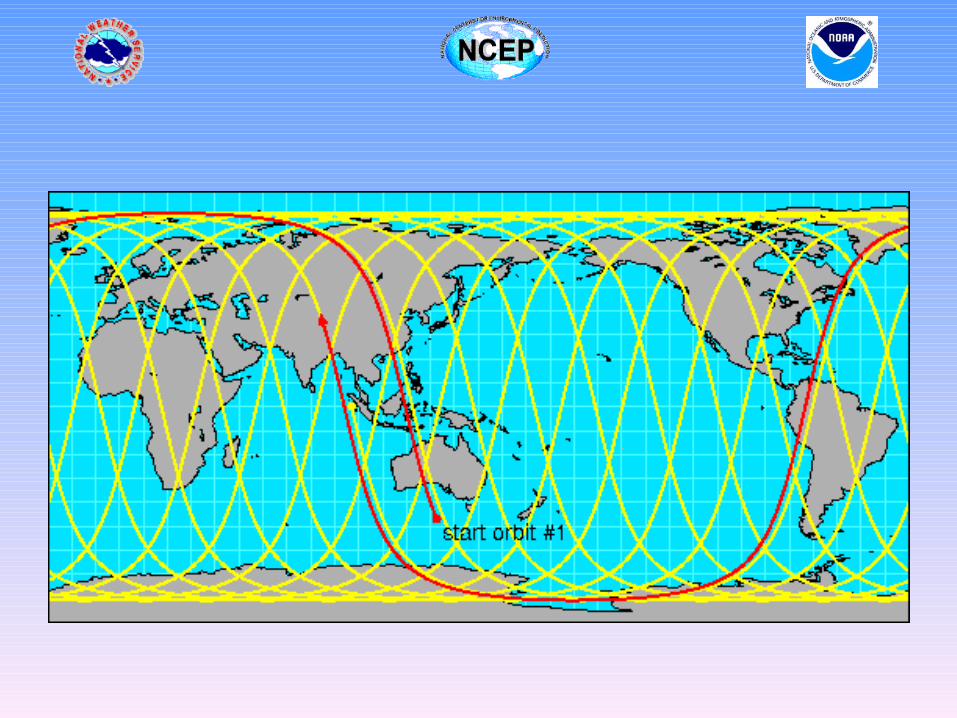
Satellite data delivery• Satellite data must wait until ground station within sight to
download• Conflicts between satellites• Blind orbits (reduced with METOP ground station)• Proposed NPOESS ground system (METOP currently left
out)– SafetyNet is a system of 15 globally distributed receptors
linked to the centrals via commercial fiber, it enables low data latency and high data availability
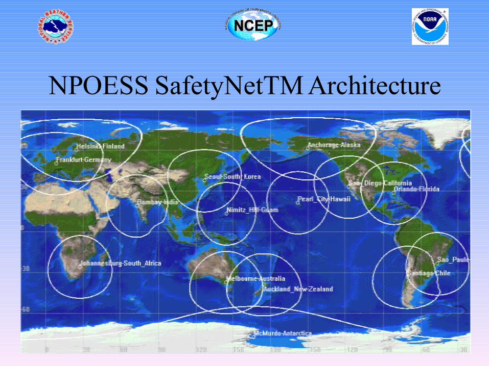
NPOESS SafetyNetTM Architecture
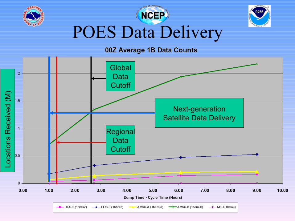
POES Data Delivery
Loca
tions
Rec
eive
d (M
)
GlobalData
Cutoff
RegionalData
Cutoff
Next-generationSatellite Data Delivery
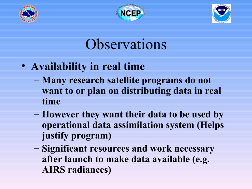
Observations• Availability in real time
– Many research satellite programs do not want to or plan on distributing data in real time
– However they want their data to be used by operational data assimilation system (Helps justify program)
– Significant resources and work necessary after launch to make data available (e.g. AIRS radiances)
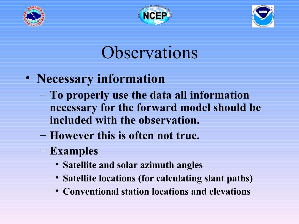
Observations• Necessary information
– To properly use the data all information necessary for the forward model should be included with the observation.
– However this is often not true. – Examples
• Satellite and solar azimuth angles• Satellite locations (for calculating slant paths)• Conventional station locations and elevations
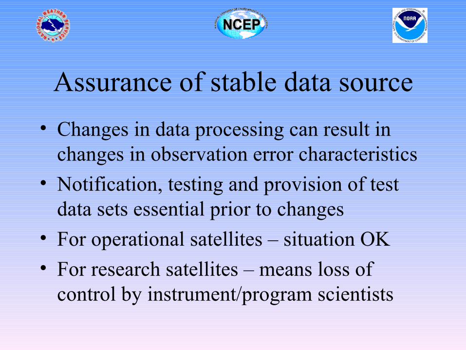
Assurance of stable data source
• Changes in data processing can result in changes in observation error characteristics
• Notification, testing and provision of test data sets essential prior to changes
• For operational satellites – situation OK
• For research satellites – means loss of control by instrument/program scientists
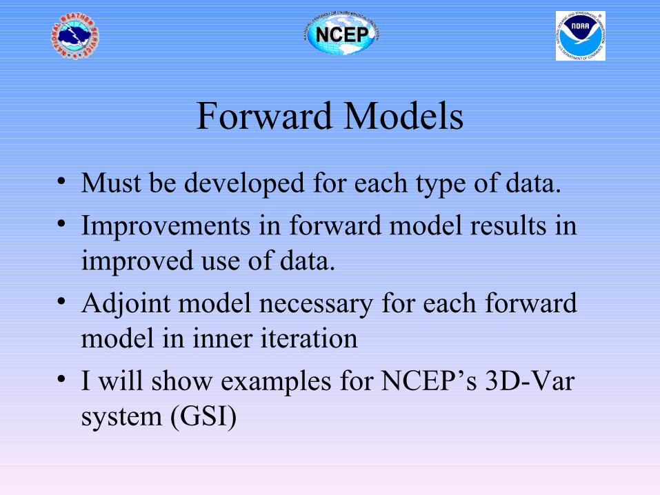
Forward Models
• Must be developed for each type of data.
• Improvements in forward model results in improved use of data.
• Adjoint model necessary for each forward model in inner iteration
• I will show examples for NCEP’s 3D-Var system (GSI)
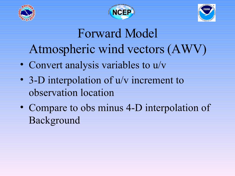
Forward ModelAtmospheric wind vectors (AWV)
• Convert analysis variables to u/v
• 3-D interpolation of u/v increment to observation location
• Compare to obs minus 4-D interpolation of Background
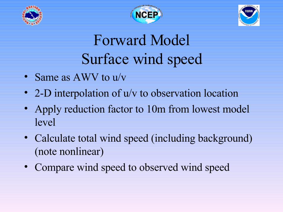
Forward ModelSurface wind speed
• Same as AWV to u/v• 2-D interpolation of u/v to observation location• Apply reduction factor to 10m from lowest model
level• Calculate total wind speed (including background)
(note nonlinear)• Compare wind speed to observed wind speed
Forward ModelScatterometer
• Same as AWV to u/v• 2-D interpolation of u/v to observation location • Apply reduction factor to 10m from lowest model
level• Compare u/v to observed u/v• Note forward model could/should be more complex
because of ambiguity in wind vectors – use backscatter directly? – difficulties in defining observational error

Forward ModelGPS radio-occultation
• Convert analysis variables to T, q, p• Interpolate T,q and p to profiles at observation
location• Calculate either refractivity or bending angle
– Tangent linear if inner iteration– Refractivity:– Bending Angle:
• Compare to observation
)/(1073.3)/(6.77 25 TPxTPN v+=
dxax
dxndaaa∫∞
−−=
2/122 )(
/ln2)(α
Forward ModelPrecipitation observations
• Convert analysis variables to T, q, Ps, u, v, cloud liquid water
• Interpolate T, q, u, and v profiles and Ps to observation location
• Calculate estimate of precipitation from model precipitation parameterization– Tangent linear of calculation – inner iteration– Need to upgrade to current version of model physics– Note when estimate of precip is negative must be set to zero
• Compare log observation to log of estimate
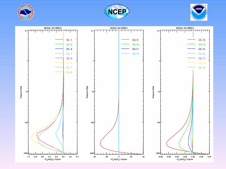
Forward ModelSBUV ozone profiles
• Convert analysis variables to ozone
• Interpolate ozone profile to observation location
• Integrate ozone profile over layers represented by observations
• Compare layer observations to simulated ozone observations
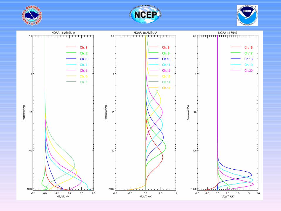
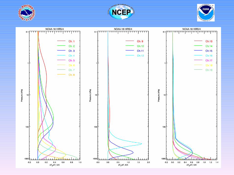
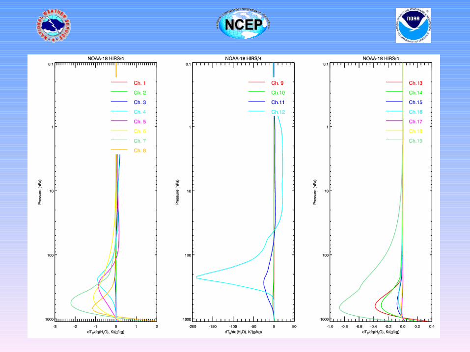
Forward ModelRadiances
• Convert analysis variables to T, q, Ps, u, v, ozone• Interpolate T profiles, q profiles, ozone profiles, u1,v1, Ps and
other surface quantities to observation location• Reduce u1 and v1 to 10m values
• Calculate estimate of radiance using radiative transfer model (and surface emissivity model)– Tangent linear of calculation – inner iteration– Currently simulation does not include clouds
• Apply bias correction• Compare observation to estimate

Radiative Transfer Model
• Community Radiative Transfer Model
• The CRTM is being developed as the basis for the use of satellite data at NCEP (and other locations).
• The radiative transfer problem is split into various components (e.g. gaseous absorption, scattering etc) to facilitate independent development.
• Want to minimise or eliminate potential software conflicts and redundancies.
• Components developed by different groups can “simply” be dropped into the framework.
• Faster implementation of new science/algorithms.
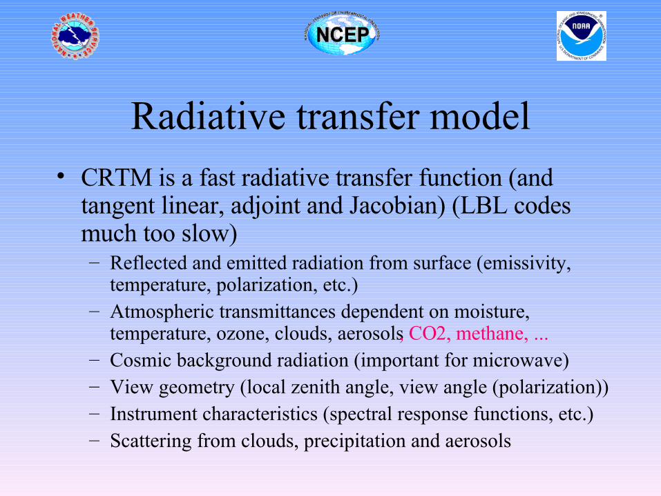
Radiative transfer model• CRTM is a fast radiative transfer function (and
tangent linear, adjoint and Jacobian) (LBL codes much too slow)– Reflected and emitted radiation from surface (emissivity,
temperature, polarization, etc.)– Atmospheric transmittances dependent on moisture,
temperature, ozone, clouds, aerosols, CO2, methane, ...– Cosmic background radiation (important for microwave)– View geometry (local zenith angle, view angle (polarization))– Instrument characteristics (spectral response functions, etc.)– Scattering from clouds, precipitation and aerosols
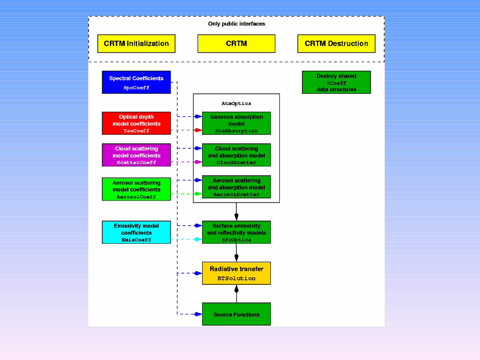
CRTM Schematic
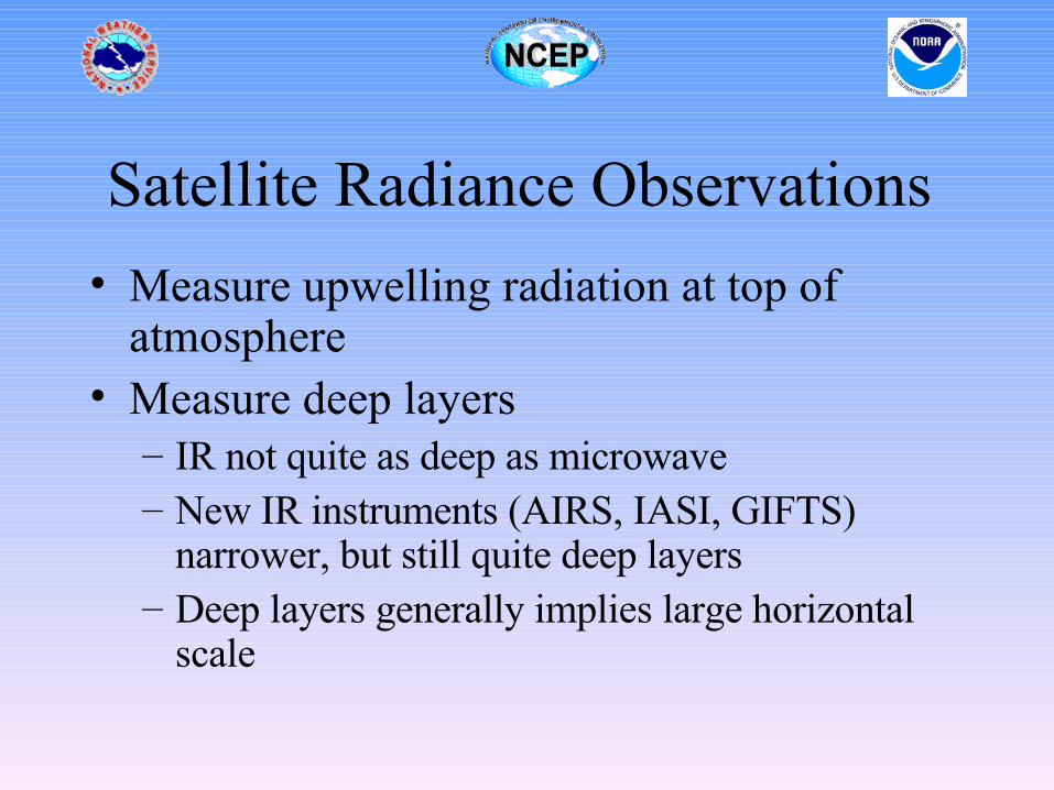
Satellite Radiance Observations
• Measure upwelling radiation at top of atmosphere
• Measure deep layers – IR not quite as deep as microwave– New IR instruments (AIRS, IASI, GIFTS)
narrower, but still quite deep layers– Deep layers generally implies large horizontal
scale
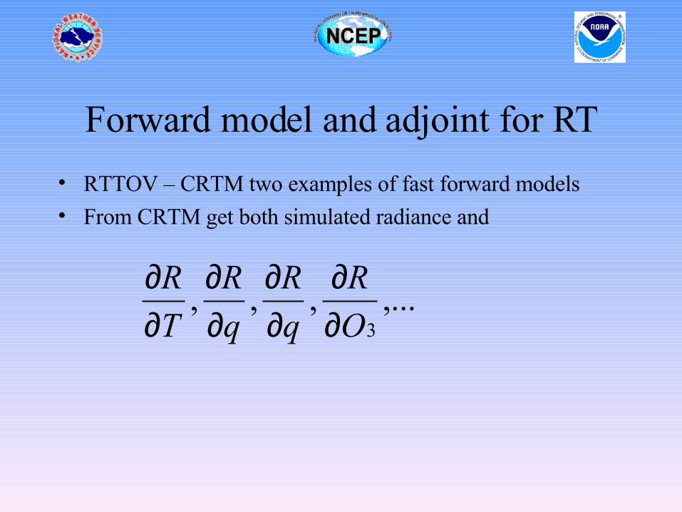
Forward model and adjoint for RT
• RTTOV – CRTM two examples of fast forward models• From CRTM get both simulated radiance and
,...,,,3O
R
q
R
q
R
T
R
∂∂
∂∂
∂∂
∂∂
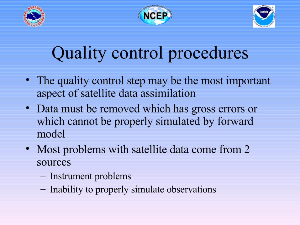
Quality control procedures• The quality control step may be the most important
aspect of satellite data assimilation• Data must be removed which has gross errors or
which cannot be properly simulated by forward model
• Most problems with satellite data come from 2 sources– Instrument problems– Inability to properly simulate observations
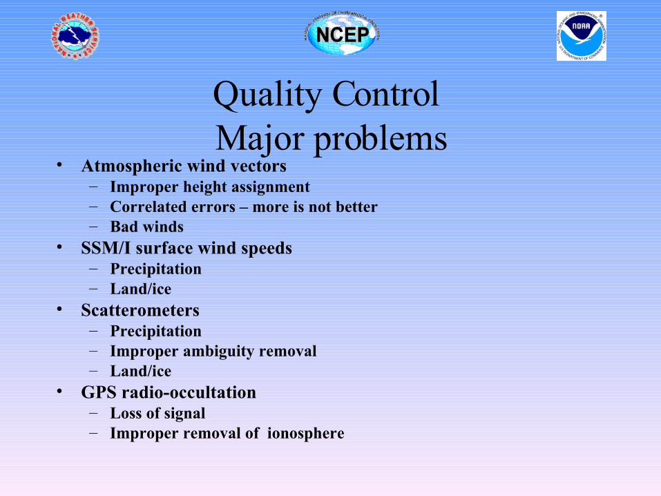
Quality Control Major problems
• Atmospheric wind vectors– Improper height assignment– Correlated errors – more is not better– Bad winds
• SSM/I surface wind speeds– Precipitation– Land/ice
• Scatterometers– Precipitation– Improper ambiguity removal– Land/ice
• GPS radio-occultation– Loss of signal– Improper removal of ionosphere
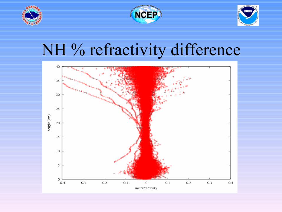
NH % refractivity difference
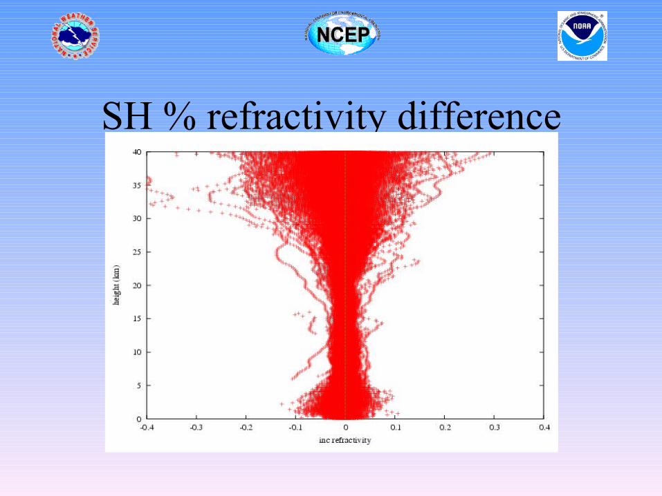
SH % refractivity difference
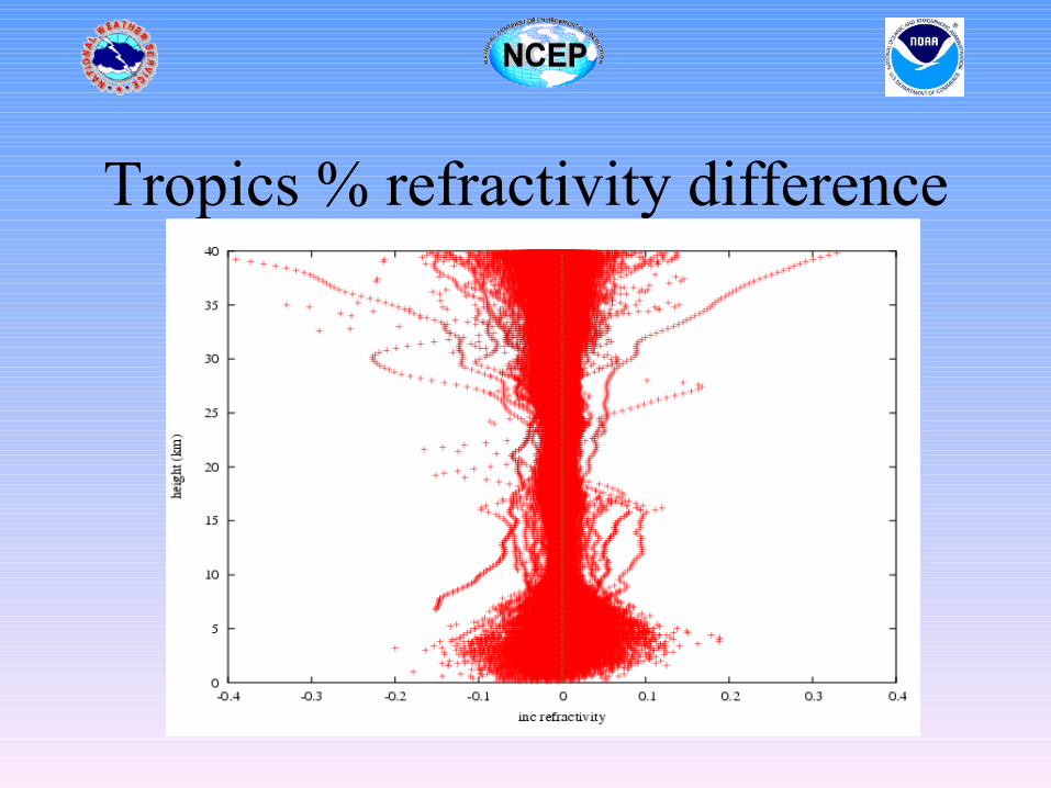
Tropics % refractivity difference
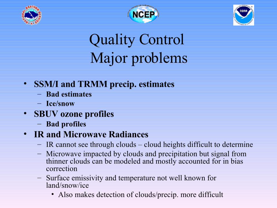
Quality Control Major problems
• SSM/I and TRMM precip. estimates– Bad estimates– Ice/snow
• SBUV ozone profiles– Bad profiles
• IR and Microwave Radiances– IR cannot see through clouds – cloud heights difficult to determine– Microwave impacted by clouds and precipitation but signal from
thinner clouds can be modeled and mostly accounted for in bias correction
– Surface emissivity and temperature not well known for land/snow/ice
• Also makes detection of clouds/precip. more difficult
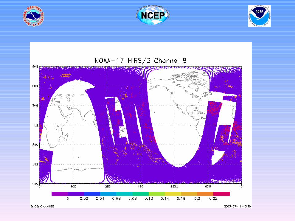
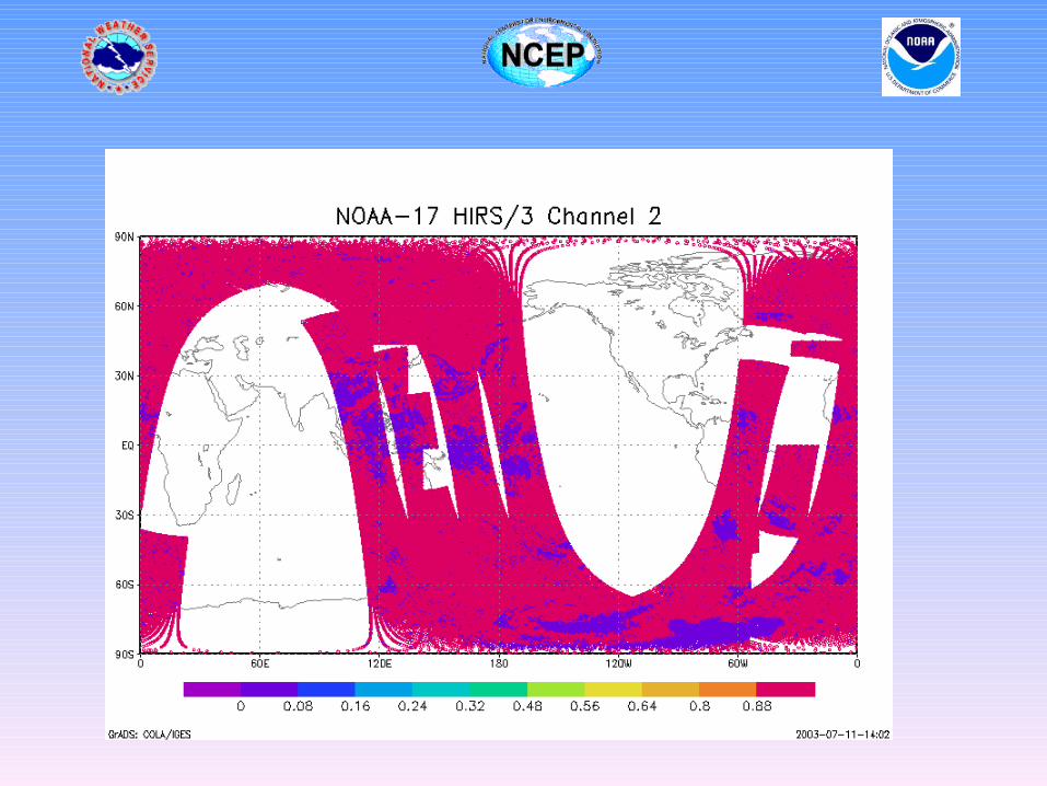
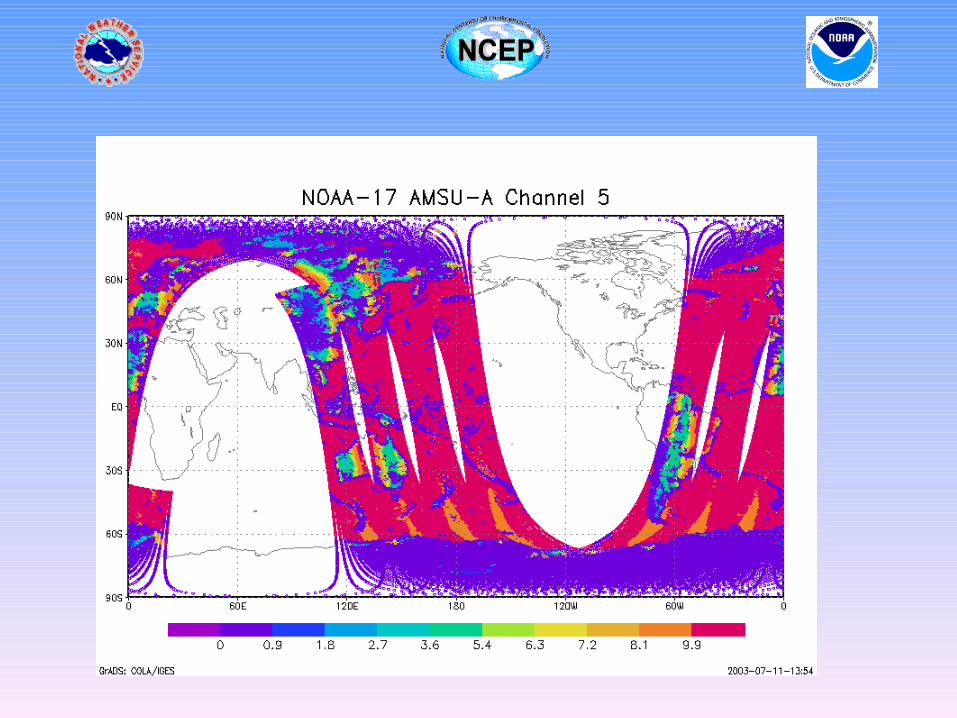
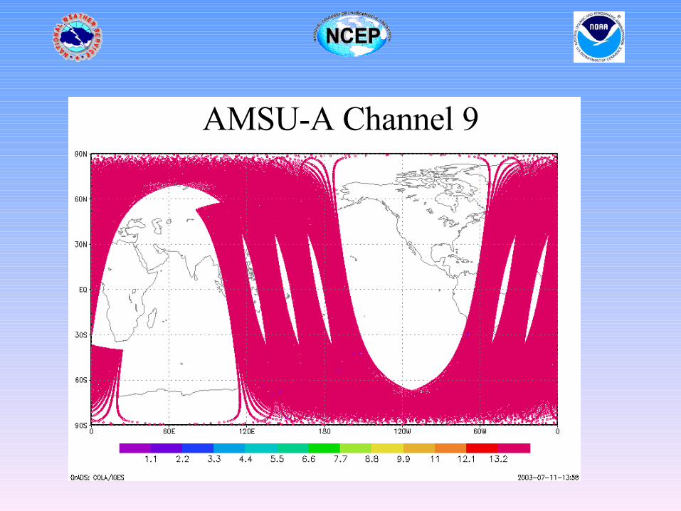
AMSU-A Channel 9
Quality control procedures(thinning)
• Some data is thinned prior to using• Three reasons
– Redundancy in data• Radiances
• AMWs
– Reduce correlated error• AMWs
– Computational expense• Radiances
Observational and Representativeness error
• Essentially specifies the weight given an observation.
• Current assumption – errors are uncorrelated– Some error specifications (e.g., radiances) increased
because of this.
• Includes instrument error, forward model error and representativeness error
Observational and Representativeness errors
• Specified somewhat empirically. – Errors quoted by instrument developers - lower bound– Fits to observations to simulated observations – upper bound– Specification of errors can be verified with some necessary
conditions in analysis system
• Generally for satellite data errors are specified a bit large since the correlated errors are not well known.
• Bias must be accounted for since it is often larger than signal
Satellite observations
• Different observation and error characteristics– Type of data (cloud track winds, radiances, etc.) – Version of instrument type (e.g., IR sounders
-AIRS, HIRS, IASI, GOES, GIFTS, etc.)– Different models of same instrument (e.g.,
NOAA-15 AMSU-A, NOAA-16 AMSU-A)
Bias Correction• The differences between simulated and observed
observations can show significant biases• The source of the bias can come from
– Biased observations– Inadequacies in the characterization of the instruments– Deficiencies in the forward models– Biases in the background
• Except when the bias is due to the background we would like to remove these biases
Bias Correction• Currently we are only bias correcting, the radiances and the
radiosonde data (radiation correction)• For radiances, biases can be much larger than signal.
Essential to bias correct the data• NCEP uses a 2 step process for radiances (others are
similar)– Angle correction (very slowly evolving – different correction for
each scan position)– Air Mass correction (slowly evolving based on predictors)
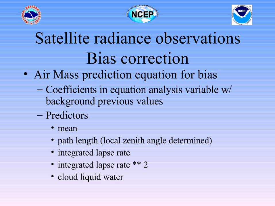
Satellite radiance observationsBias correction
• Air Mass prediction equation for bias– Coefficients in equation analysis variable w/
background previous values– Predictors
• mean• path length (local zenith angle determined)• integrated lapse rate• integrated lapse rate ** 2• cloud liquid water
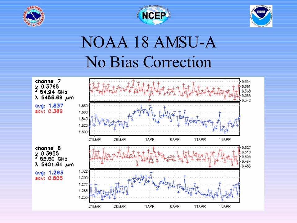
NOAA 18 AMSU-ANo Bias Correction
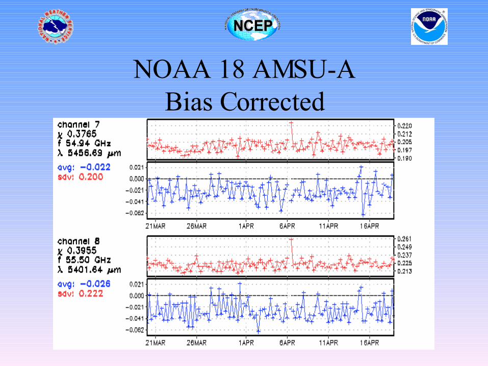
NOAA 18 AMSU-ABias Corrected
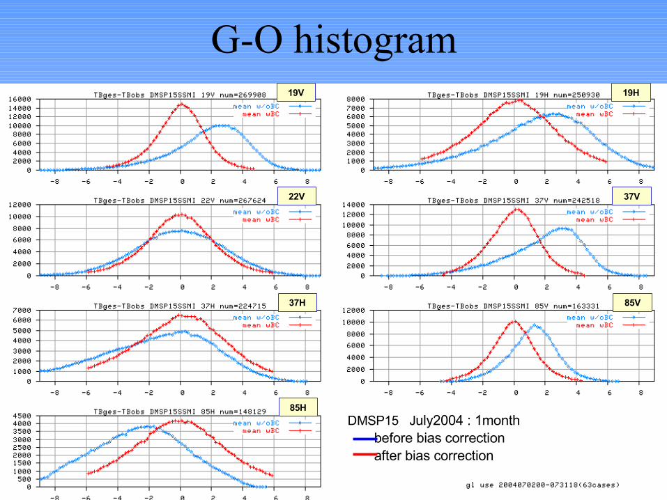
G-O histogram
DMSP15 July2004 : 1month before bias correction after bias correction
19V
22V
19H
37V
37H
85H
85V
Data Monitoring
• It is essential to have good data monitoring.
• Usually the NWP centres see problems with instruments prior to notification by provider (UKMO especially)
• The data monitoring can also show problems with the assimilation systems
• Needs to be ongoing/real time
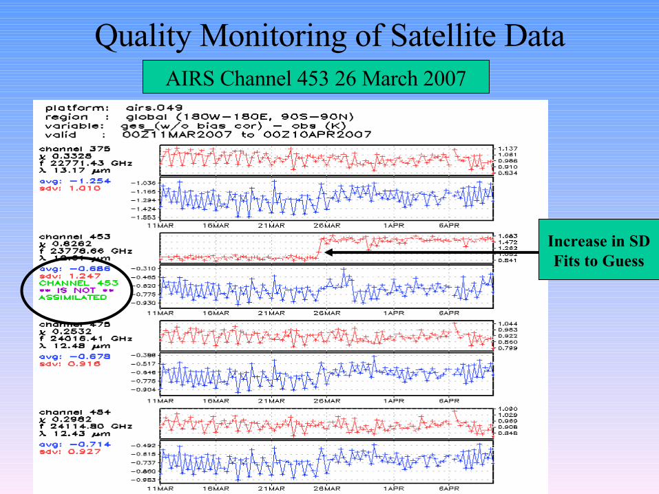
Quality Monitoring of Satellite DataAIRS Channel 453 26 March 2007
Increase in SDFits to Guess
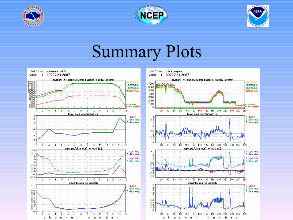
Summary Plots
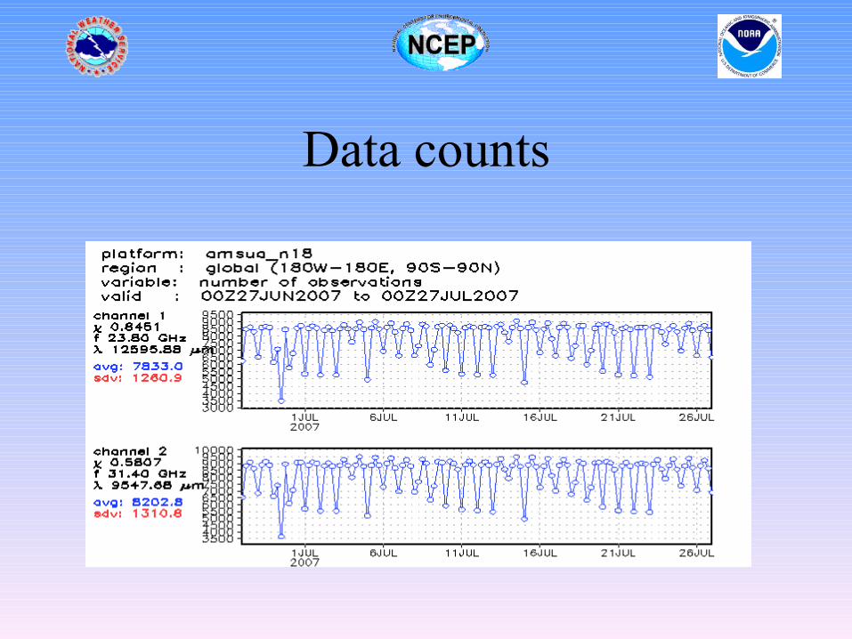
Data counts
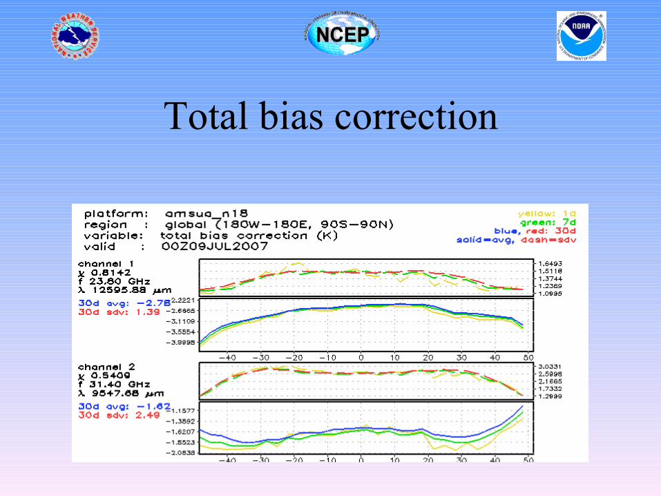
Total bias correction
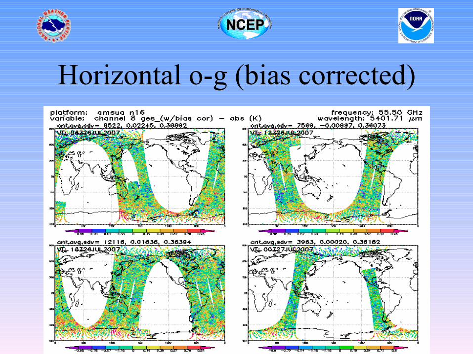
Horizontal o-g (bias corrected)
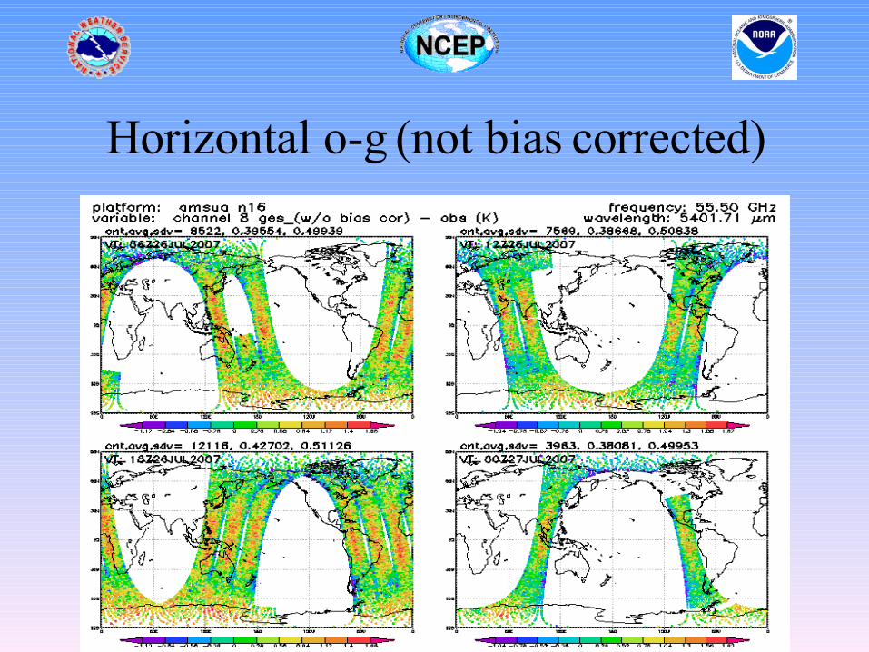
Horizontal o-g (not bias corrected)
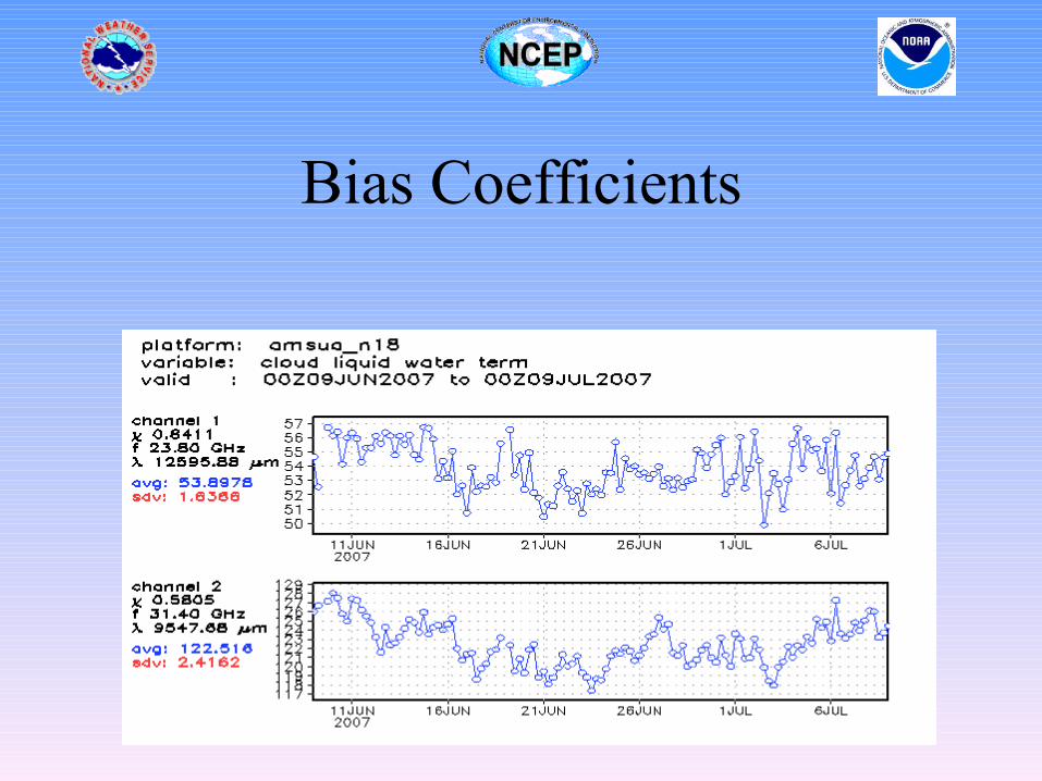
Bias Coefficients
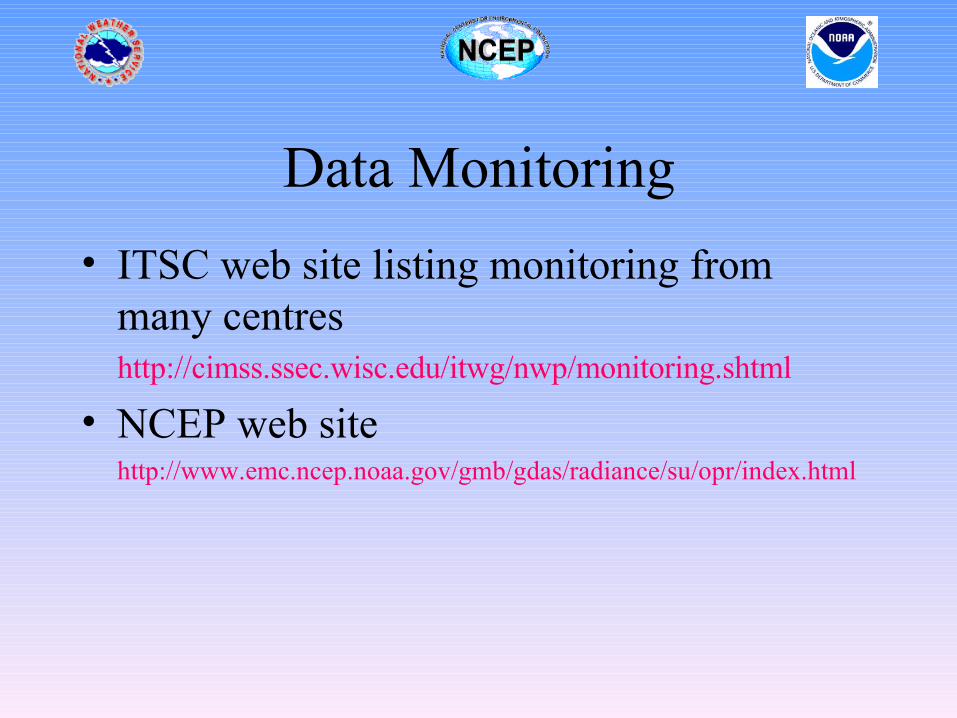
Data Monitoring
• ITSC web site listing monitoring from many centreshttp://cimss.ssec.wisc.edu/itwg/nwp/monitoring.shtml
• NCEP web site http://www.emc.ncep.noaa.gov/gmb/gdas/radiance/su/opr/index.html
Data impact
• Satellite data extremely important part of observation system.
• Much of the improvement in forecast skill can be attributed to the improved data and the improved use of the data
• Must be measured relative to rest of observing system – not as stand alone data sets
• Extremely important for planning ($$$$)
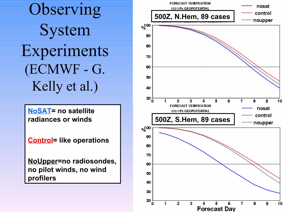
Observing System
Experiments(ECMWF - G.
Kelly et al.)
500Z, N.Hem, 89 cases
500Z, S.Hem, 89 casesNoSAT= no satellite radiances or winds
Control= like operations
NoUpper=no radiosondes, no pilot winds, no wind profilers
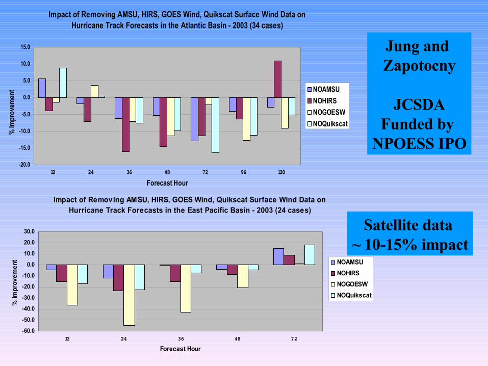
Jung and Zapotocny
JCSDAFunded by
NPOESS IPO
Satellite data ~ 10-15% impact
Impact of Removing AMSU, HIRS, GOES Wind, Quikscat Surface Wind Data on Hurricane Track Forecasts in the Atlantic Basin - 2003 (34 cases)
-20.0
-15.0
-10.0
-5.0
0.0
5.0
10.0
15.0
12 24 36 48 72 96 120
Forecast Hour
% Im
prov
emen
t NOAMSU
NOHIRS
NOGOESW
NOQuikscat
Impact of Removing AMSU, HIRS, GOES Wind, Quikscat Surface Wind Data on Hurricane Track Forecasts in the East Pacific Basin - 2003 (24 cases)
-60.0
-50.0
-40.0
-30.0
-20.0
-10.0
0.0
10.0
20.0
30.0
12 24 36 48 72
Forecast Hour
% Im
prov
emen
t NOAMSU
NOHIRS
NOGOESW
NOQuikscat
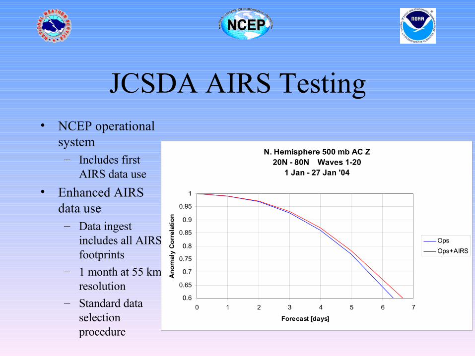
JCSDA AIRS Testing• NCEP operational
system– Includes first
AIRS data use
• Enhanced AIRS data use– Data ingest
includes all AIRS footprints
– 1 month at 55 km resolution
– Standard data selection procedure
N. Hemisphere 500 mb AC Z 20N - 80N Waves 1-20
1 Jan - 27 Jan '04
0.6
0.65
0.7
0.75
0.8
0.85
0.9
0.95
1
0 1 2 3 4 5 6 7
Forecast [days]
An
om
aly
Co
rrel
atio
n
Ops
Ops+AIRS
Summary• Operational data assimilation of satellite data
requires:– Data available in real time in acceptable format– Necessary information in data file– A stable data source– Quality control procedures to be defined– Bias correction and observational errors defined – An accurate forward model– Data monitoring– Evaluation and testing to ensure neutral/positive impact
Additional information
• International TOVS Working Group (ITWG) – just radiances but still very useful http://cimss.ssec.wisc.edu/itwg/nwp
• NOAA POES status http://www.oso.noaa.gov/poesstatus/
• NOAA GOES status http://www.oso.noaa.gov/goesstatus/
Future
• New satellite data types/uses– Imagery (especially 4D) replacing AMWs– Use of cloud information in imager/sounders– New quantities – aerosols, constituent gases,
surface parameters, etc.– Wind lidars– etc.
Future• Many new “enhanced” instruments
METOP/NPP/NPOESS• Impact experiments – must be done well
– All other observations used– Accuracy of:
• Forecast model• Observations• Simulations of observations• Statistical formulations for errors
– Computing Capability (Determines sophistication of assimilation techniques)
Metop-A (Metop-2)• Launched 19 October 2006• Instruments
– AMSU-A (Advanced Microwave Sounding Units)– MHS (Microwave Humidity Sounder)– HIRS-4 (High-resolution Infrared Radiation Sounding)– IASI (Infrared Atmospheric Sounding Interferometer)– GOME-2 (Global Ozone Monitoring Experiment)– GRAS (Global navigation satellite system reciever for
Atmospheric Sounding)– ASCAT (Advanced Scatterometer)– AVHRR (Advanced Very High Resolution Radiometer)
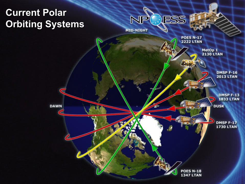
Current Polar Current Polar Orbiting SystemsOrbiting Systems

Metop-A (Metop-2)
• Heritage Instruments– AMSU-A– HIRS-4– AVHRR– MHS – Operationally using AMSU, HIRS, MHS
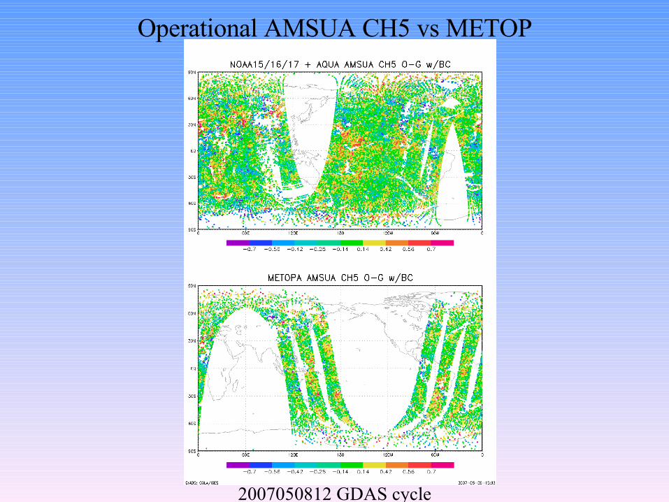
Operational AMSUA CH5 vs METOP
2007050812 GDAS cycle
Metop-A (Metop-2)
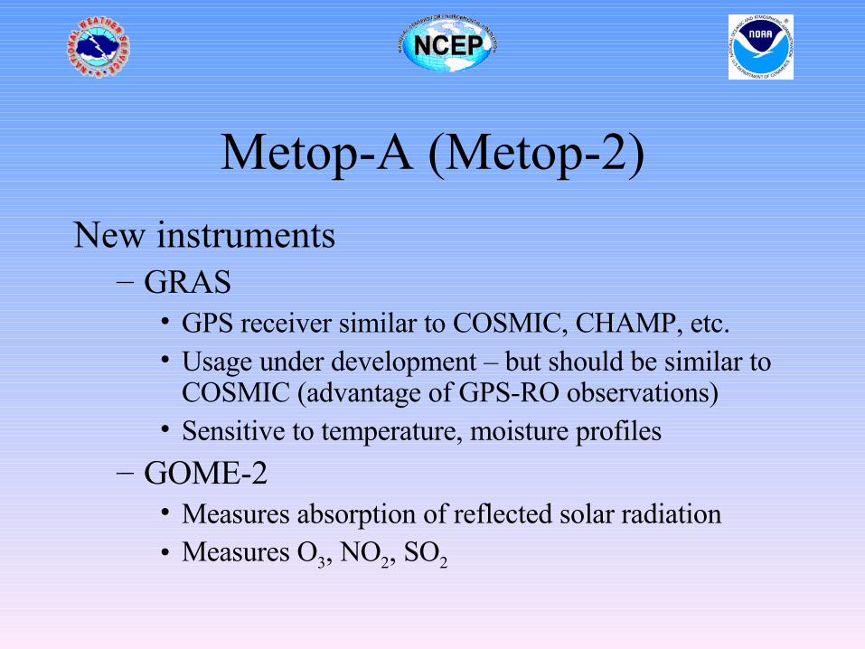
New instruments– GRAS
• GPS receiver similar to COSMIC, CHAMP, etc.• Usage under development – but should be similar to
COSMIC (advantage of GPS-RO observations)• Sensitive to temperature, moisture profiles
– GOME-2• Measures absorption of reflected solar radiation• Measures O3, NO2, SO2
Metop-A (Metop-2)
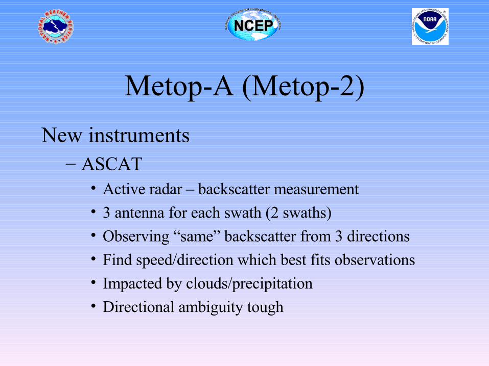
New instruments– ASCAT
• Active radar – backscatter measurement• 3 antenna for each swath (2 swaths)• Observing “same” backscatter from 3 directions• Find speed/direction which best fits observations• Impacted by clouds/precipitation• Directional ambiguity tough
Metop-A (Metop-2)
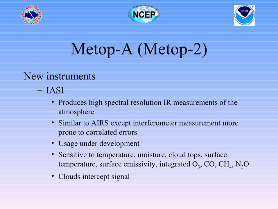
New instruments– IASI
• Produces high spectral resolution IR measurements of the atmosphere
• Similar to AIRS except interferometer measurement more prone to correlated errors
• Usage under development
• Sensitive to temperature, moisture, cloud tops, surface temperature, surface emissivity, integrated O3, CO, CH4, N2O
• Clouds intercept signal
NPOESS Preparatory Project (NPP)
• Transition mission between DMSP/NOAA and NPOESS
• Major instruments from NPOESS (without improved communication)
• Still changing
• Launch date “about 2009”
NPOESS Preparatory Project (NPP)
• Instruments– VIIRS (Visible/Infrared Imager/Radiometer
Suite)• Higher resolution/more bands version of AVHRR
– ATMS (Advanced Technology Microwave Sounder)
• Similar to AMSU-A/B – MHS (with 2 more channels)
NPOESS Preparatory Project (NPP)
• Instruments– CrIS (Cross-track Infrared Sounder)
• Interferometer based (more correlated errors?)• Clouds
– OMPS (Ozone Mapping and Profiler Suite )• Measures along-track limb scattered solar radiance • Scanning instrument provides profiles of ozone
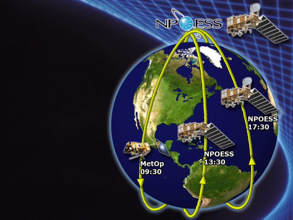
NPOESS
• National Polar-Orbiting Operational Environmental Satellite System ( NPOESS)
• Contains NPP instruments + – Perhaps a conical scanning microwave
instrument
• Troubled program – additional changes likely in my opinion
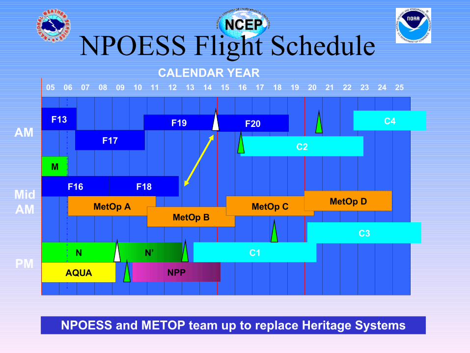
NPOESS Flight Schedule
F17
F19
F18
F20
F16
F13
M
N N’
NPP
MetOp AMetOp B
MetOp C
C1
C2
C3
AM
MidAM
PM
05 06 07 08 09 11 12 13 14 15 16 17 18 19 20 21 22 23 24 2510
AQUA
MetOp D
C4
CALENDAR YEAR
NPOESS and METOP team up to replace Heritage Systems
Future• Rational decision process for observing system
design – Politics and money are important for satellite data– How to determine relative importance for new
instruments?– OSSEs?
• Tremendous volume of satellite data coming in the future from a wide variety of instruments
• Development of the proper data handling systems and models to simulate this data will be necessary
Final Comments
• The presence of satellite has virtually eliminated data voids.• Satellite data must be used carefully because of biases or
correlated errors in the data or processing.• Still lots of work to be done
– Difficult to even keep up with current programs• At NCEP we currently have projects underway to use:
– METOP IASI– AVHRR– GOES imagery– AMSR-E– SSM/IS radiances
Final Comments(Opinion based on experience)
• For NWP, satellite radiances most important satellite observation – Microwave radiances more useful than IR radiances because of
clouds• More observations are not always better• Impact of new instruments never as large as predicted by
instrument advocates– Instruments justified based on NWP impacts
• Larger improvement usually occurs because of improvement to assimilation systems than the addition of new data
Final Comments(Opinion based on experience)
• Most applied research in atmospheric data assimilation done at operational centers (and GSFC DAO)
• Much of expertise and knowledge is undocumented or minimally documented – papers are not the priority at operational centers
• Many opportunities to use new observations and to improve forward models for DA.
• Data assimilation is where everything comes together– To use new observations properly requires one to become an
expert in that particular instrument– One must be knowledgeable on forecast model dynamics and
physics to understand background errors– Computational techniques are necessary to improve efficiency
Final Comments(Opinion based on experience)
• Very few satellite programs justified by their impact on data assimilation actually account for data assimilation in their program– Cost and time necessary to assimilate data– Necessary data communication and data formatting problems– Impact on computing resources– AIRS and COSMIC exceptions
• To properly provide data assimilation input to satellite programs is a huge time investment.– There are an infinite number of satellite meetings
Final Comments(Opinion based on experience)
• It is great to be involved in the operational side of data assimilation – it allows you to see the data used and have an impact!