Satellite Communications - LTAS-SDRG Communications ... Link budget Marc Van ... Main type s of satellite ! di erent types of information Astronomical satellites:

Signal processing elementsPropagation and radio communications

Engineering

Satellite Communications

Marc Van Droogenbroeck

Department of Electrical Engineering and Computer ScienceUniversity of Liège

Academic year 2016-2017

Marc Van Droogenbroeck Satellite Communications


Engineering

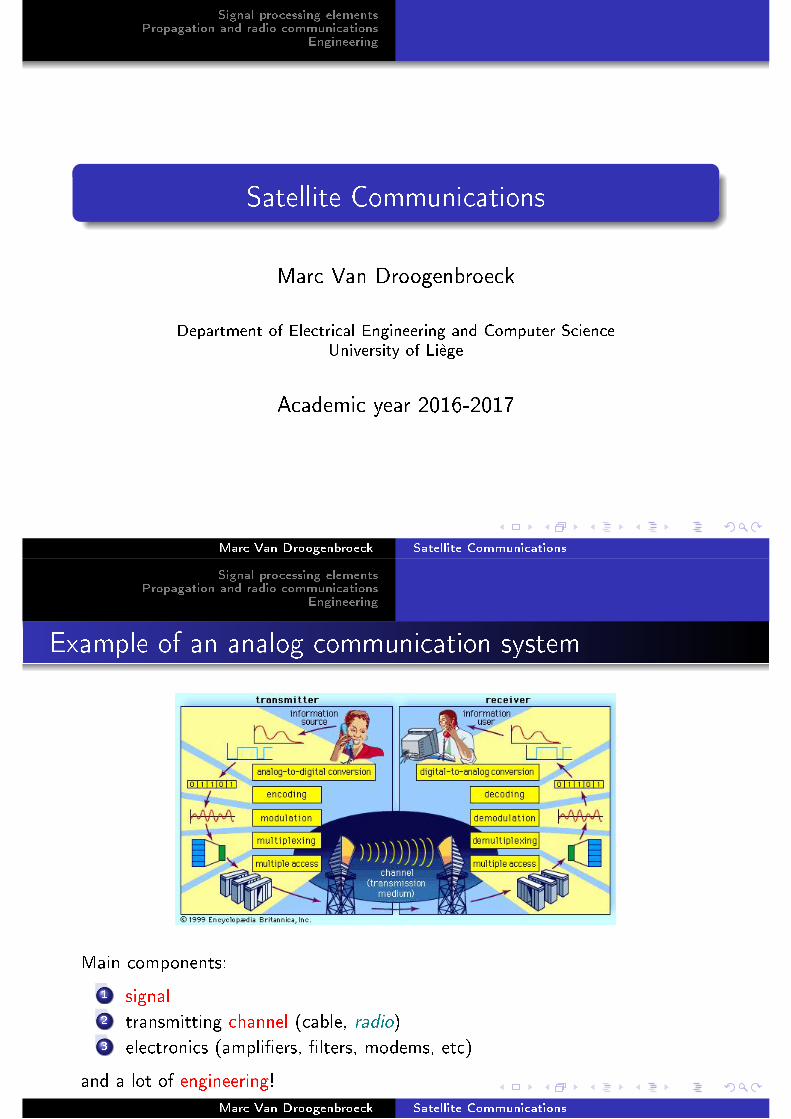
Example of an analog communication system

Main components:

1 signal2 transmitting channel (cable, radio)3 electronics (ampli�ers, �lters, modems, etc)

and a lot of engineering!



Engineering

Outline

1 Signal processing elements

Signal ≡ information!

Source coding (dealing with the information content)

Modulation

Multiplexing

2 Propagation and radio communications

Introduction to radio communications

Radiowave propagation

Examples of antennas

3 Engineering

Noise

Link budget



Engineering

Signal ≡ information!Source coding (dealing with the information content)ModulationMultiplexing

Outline




Modulation

Multiplexing





3 Engineering

Noise

Link budget



Engineering


Main types of satellite → di�erent types of information

Astronomical satellites: used for observation of distant planets,galaxies, and other outer space objects.

Navigational satellites [GPS, Galileo]: they use radio timesignals transmitted to enable mobile receivers on the ground todetermine their exact location (positioning).

Earth observation satellites: used for environmentalmonitoring, meteorology, map making.

Miniaturized satellites: satellites of unusually low masses andsmall sizes. For example, for educational purposes (OUFTI-1).

Communications satellites: stationed in space for the purposeof telecommunications. Modern communications satellitestypically use geosynchronous orbits, or Low Earth orbits (LEO).


Example: constellation of GPS satellites

6 planes with a 55° angle with the equator, spaced by 60° and with 4satellites per plane (24 satellites in total)

Located on high orbits (but sub-geostationary)/revolution in 12 hours

Transmitting power of 20 to 50 [W]

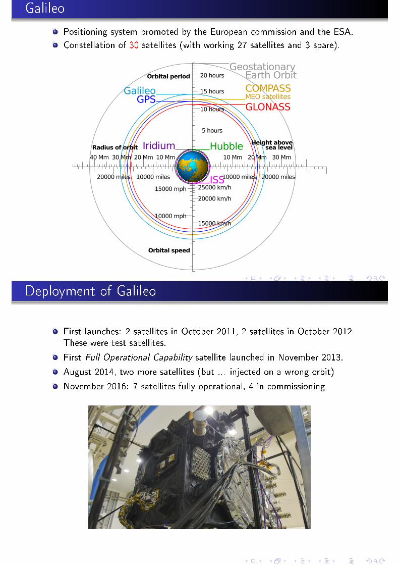
Galileo

Positioning system promoted by the European commission and the ESA.

Constellation of 30 satellites (with working 27 satellites and 3 spare).

GeostationaryEarth Orbit

GPSGLONASS

Galileo COMPASSMEO satellites

Iridium Hubble

ISS

Radius of orbit

10 Mm20 Mm30 Mm40 Mm

10000 miles20000 miles

Height abovesea level

10 Mm 20 Mm 30 Mm

10000 miles 20000 miles

Orbital period

5 hours

10 hours

15 hours

20 hours

Orbital speed

25000 km/h

20000 km/h

15000 km/h

15000 mph

10000 mph

Deployment of Galileo

First launches: 2 satellites in October 2011, 2 satellites in October 2012.These were test satellites.

First Full Operational Capability satellite launched in November 2013.

August 2014, two more satellites (but ... injected on a wrong orbit)

November 2016: 7 satellites fully operational, 4 in commissioning

Types of data streams

Types of data Characteristics

Control data Must be very reliable

Payload Unicast communication for mobile ground station

. Measurements Accurate signals with constant monitoring

. Remote sensing data High volume of downstream data

. Localization data Accurate time reference (synchronization)

. Broadcasting Digital television channels

. Digital data Voice + data (Internet) for remote areas

Because the purposes of data sent are di�erent, the mechanisms totransmit the data are designed according to the constraints.

Simpli�ed typography of data streams:

control data

payload (+ some unavoidable overhead)


Engineering


Main concerns related to signals

Signal source handling (preparation of the signal, at thesource, in the transmitter):

�ltering (remove what is useless for communications)analog ↔ digital (digitization)remove the redundancy in the signal: compression

Signal over the channel:

signal shaping to make it suitable for transmission (coding,modulation, multiplexing, etc)signal power versus the noise signal (protect the signal againstnoise e�ects)



Engineering


Digitization I



Engineering


Digitization II

Digitization = from analog to digital

analog digital

g(t) samples g [iT ], with

i = 0, 1, 2, . . . and T ,

a time period

signal over time sampling rate

set of samples

each sample is coded

with n bits

(quantization)

in the end, we have a

bitsream: 01110...



Engineering


Digitization III

Digitization in numbers:

1 fs : sampling frequency

Let W be the highest frequency of the signal to be convertedtheoretical lower bound: fs > 2Wpractical rule (Nyquist criterion): fs > 2.2W

2 n: number of bits par sample (quantization)3 bit rate = fs × n

signal band W fs n bit rate

units Hz Hz sample/s b/sa. b/s

audio

(telephone)

[300 Hz,

3400 Hz]

3400 Hz 8000 sa./s 8 64 kb/s

audio (CD) [0 Hz, 20 kHz] 20 kHz 44.1 ksa./s 16 705.6 kb/s



Engineering


Analog and digital signals: don't confuse information and itsrepresentation!

1 0 1 0 1 1

Analog information signal Digital information signal

Analog representation Analog representation

-1

-0.5

0

0.5

1

1.5

2

0 2 4 6 8 10

-2

-1.5

-1

-0.5

0

0.5

1

1.5

2

0 2 4 6 8 10-0.5

0

0.5

1

1.5

0 1 2 3 4 5 6-1.5

-1

-0.5

0

0.5

1

1.5

0 1 2 3 4 5 6


Characterization of signals over the channel

Analog signal Digital signal

bandwidth [Hz] bit rate [bit/s]

Signal to Noise Ratio (S/N or SNR) Bit Error Rate (BER)

bandwidth of the underlying channel [Hz]

Reasons for going digital:

possibility to regenerate a digital signal

better bandwidth usage

Example (better bandwidth usage: from analog to digital television)

analog PAL television channel: bandwidth of 8 [MHz]

digital television, PAL quality ∼ 5 [Mb/s]

With a 64-QAM modulation, whose spectral e�ciency is 6b/s perHz. A bandwidth of 8 [MHz] allows for 48 [Mb/s].Conclusion: thanks to digitization, there is room for 10 digitaltelevision channels instead of 1 analog television channel.

Software organization of a transmitter/receiver: the OSIreference model

Consequence: encapsulation ⇒ overhead

OSI reference model vs Internet model (+ somecorresponding Internet protocols)

Elements of a communication system I

Figure : Block diagram of a communication channel for a single signal.

Elements of a communication system II


Engineering


Outline




Modulation

Multiplexing





3 Engineering

Noise

Link budget



Engineering


Information theory and channel capacity: there is maximum

bit rate! I

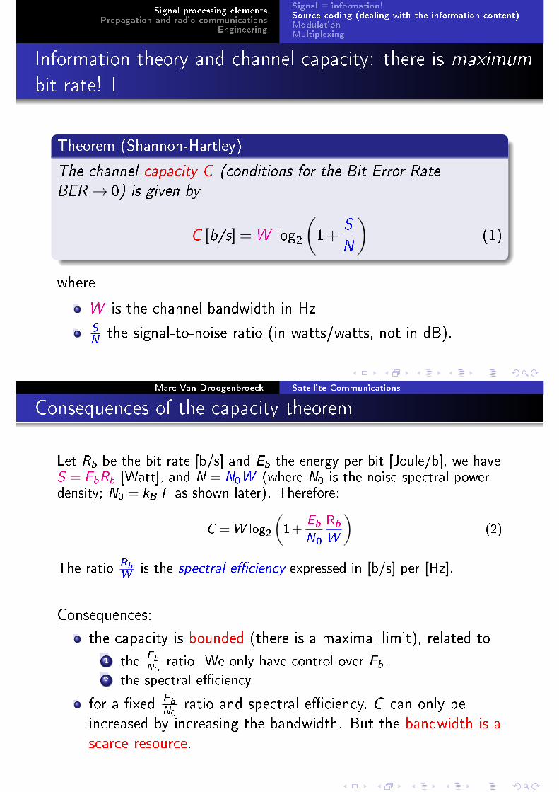
Theorem (Shannon-Hartley)

The channel capacity C (conditions for the Bit Error RateBER → 0) is given by

C [b/s] =W log2

(1+

S

N

)(1)

where

W is the channel bandwidth in HzSN

the signal-to-noise ratio (in watts/watts, not in dB).


Consequences of the capacity theorem

Let Rb be the bit rate [b/s] and Eb the energy per bit [Joule/b], we haveS = EbRb [Watt], and N = N0W (where N0 is the noise spectral powerdensity; N0 = kBT as shown later). Therefore:

C =W log2

(1+

EbN0

RbW

)(2)

The ratio Rb

Wis the spectral e�ciency expressed in [b/s] per [Hz].

Consequences:

the capacity is bounded (there is a maximal limit), related to

1 the Eb

N0ratio. We only have control over Eb.

2 the spectral e�ciency.

for a �xed EbN0

ratio and spectral e�ciency, C can only beincreased by increasing the bandwidth. But the bandwidth is ascarce resource.

Impact of errors on the transmission: bit/packet error rate

Assume a packet of size N and let Pe be the probability error on one bit(≡ Bit Error Rate, BER).

The probability for the packet to be correct is

(1−Pe)N . (3)

Therefore the packet error rate is

PP = 1− (1−Pe)N . (4)

For large packets and small Pe , this becomes

PP ' 1− (1−NPe) = N×Pe . (5)

Example

With N = 105 bits and a bit error rate of Pe = 10−7, PP ' 10−2.

We thus need to lower Pe ⇒ error detection/correction mechanisms

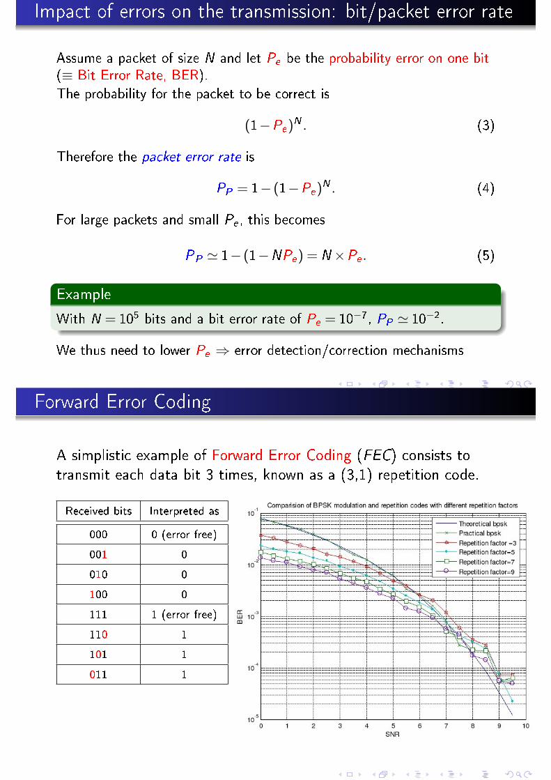
Forward Error Coding

A simplistic example of Forward Error Coding (FEC) consists totransmit each data bit 3 times, known as a (3,1) repetition code.

Received bits Interpreted as

000 0 (error free)

001 0

010 0

100 0

111 1 (error free)

110 1

101 1

011 1

Other forward error codes

Hamming code

Reed�Solomon code

Turbo code, ...


Engineering


Outline




Modulation

Multiplexing





3 Engineering

Noise

Link budget



Engineering


Modulation: principles

Principle

Modulation is all about using of a carrier cosine at frequency fc fortransmitting information. The carrier is Ac cos(2πfct)

Amplitude

s(t) = A(t)cos(2πf (t)t+φ (t))

Phase

Frequency modulation [FM]

Phase modulation [PM]Amplitude modulation [AM]


Consequences of modulation

frequency band is shifted towards the carrier frequency (⇒ fc)

bandwidth modi�cation, compared to that of the modulatingsignal m(t)

E�ects of Amplitude Modulation on the spectrum ( s(t) = Acm(t)cos(2πfc t) )

f

Ac2 δ (f + fc)

Ac2 δ (f − fc)

LSB

USB

LSBUSB

−W 0 +W

0

(b)

(a)

−fc +W−fc−fc −W fc +Wfcfc −Wf

‖M (f )‖

‖S (f )‖

Demodulation of an AM modulated signal: principles

Received signal: s(t) =m(t)cos(2πfct). Task: recover m(t).

Principles of a synchronous demodulation. At the receiver:

1 acquire a local, synchronous, copy of the carrier fc ⇒ build alocal copy of cos(2πfct)

2 multiply s(t) by cos(2πfct):[cosacosb = 1

2 cos(a−b)+ 12 cos(a+b)]

s(t)cos(2πfct) =m(t)cos2(2πfct) (6)

=m(t)[1

2+

1

2cos(2π(2fc)t)] (7)

=1

2m(t)+

1

2m(t)cos(2π(2fc)t)] (8)

3 �lter out the 2fc components → 12m(t)

Demodulation of an AM modulated signal: interpretation inthe spectral domain

fc fcff

f

f

−fc −fc

Ac/2 Ac/2 1/2 1/2

Ac/4 Ac/4

AM spectrum Spectrum of the carrier

2fc−fc fc

Ac/2

−2fc

Ac/2

Spectrum of the mixed signal

−W W

−W W

Mixer

Signal spectrum

Basic digital modulation (coding) techniques I

Basic digital modulation (coding) techniques II

Quadrature modulation

It is possible to use both a cosine and a sine:

s(t) =m1(t)cos(2πfct)−m2(t)sin(2πfct) (9)

−π2

cos(2πfc)t

sin(2πfc)t

m2(t)sin(2πfct)

m1(t)cos(2πfct)

+

−s(t)

m2(t)

m1(t)

Quadrature demodulation: principles

s(t) =m1(t)cos(2πfct)+m2(t)sin(2πfct) is the modulated signal.

We want to recover m1(t) and m2(t)

Step 1: multiply by cos(2πfct)[remember that cosa× cosb = 1

2 cos(a−b)+ 12 cos(a+b) and

that cosa× sina = 12 sin(2a)]

s(t)× cos(2πfc t) =m1(t)cos2 (2πfc t)+m2(t)sin(2πfc t)cos(2πfc t)

=1

2m1(t)+

1

2m1(t)cos(2π(2fc)t)+

1

2m2(t)sin(2π(2fc)t)

Step 2: �lter to keep the baseband signal

1

2m1(t)

Steps 3 and 4: multiply by sin(2πfct) and low-pass �lter to getm2(t)

Purposes of the quadrature modulation

There are 2 possible uses/advantages for a quadrature modulation:

1 [Bandwidth savings by a factor of 2]Send two signals in the same bandwidth

s(t) =m1(t)cos(2πfct)+m2(t)sin(2πfct) (10)

Both m1(t)cos(2πfct) and m2(t)sin(2πfct) have exactly the samebandwidth, that is [fc −W , fc +W ] where W denotes the originalbandwidth of m1(t) and m2(t).

2 [Easier demodulation]A coherent demodulation of m(t)cos(2πfct+φc) requires theperfect knowledge of fc and φc at the receiver. However, it issometimes di�cult to synchronize the receiver. Therefore,

s(t) =m(t)cos(2πfct+φc)+m(t)sin(2πfct+φc) (11)

is sometimes used.At the receiver, m(t), the signal of interest can be obtained by√m2(t)cos2(.)+m2(t)sin2(.) = |m(t)|.


Engineering


Outline




Modulation

Multiplexing





3 Engineering

Noise

Link budget



Engineering


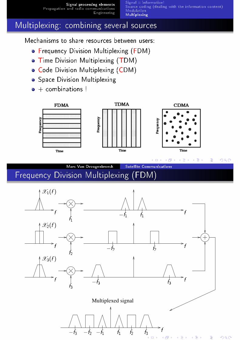
Multiplexing: combining several sources

Mechanisms to share resources between users:

Frequency Division Multiplexing (FDM)

Time Division Multiplexing (TDM)

Code Division Multiplexing (CDM)

Space Division Multiplexing

+ combinations !


Frequency Division Multiplexing (FDM)

f−f3 f3

f−f3 f3

−f2 f2

−f2 f2

−f1 f1

−f1 f1

f

f

f

X1(f )

X2(f )

X3(f )

f1

f2

f3

f

f

Multiplexed signal

Demultiplexing

f−f3 f3−f2 f2−f1 f1

Multiplexed signal

f

X3(f )

f

X2(f )

f

X1(f )

f2 f3f1

f1 f2 f3

Time Division Multiplexing (TDM)

Spread spectrum for Code Division Multiplexing

Principle of spread spectrum: multiply a digital signal with a fasterpseudo-random sequence (spreading step)

f

f

NB0t

t

t f(N+1)B0

Tb

Binary data waveform

Spreading sequence

Spread sequence

B−B 0

−NB

Tc

(one bit)

F

F

F

−(N+1)B

At the receiver, the same, synchronized, pseudo-random sequence isgenerated and used to despread the signal (despreading step)

Code Division Multiple Access

Each user is given its own code (multiple codes can be usedsimultaneously)

FrequencyTime

Code

Physical channel

User 1

User 2Free channel

Summary


Engineering

Introduction to radio communicationsRadiowave propagationExamples of antennas

Outline




Modulation

Multiplexing





3 Engineering

Noise

Link budget



Engineering


Satellite link de�nition


Frequency bands

But it is also common to designate the carrier frequency andbandwidth directly.

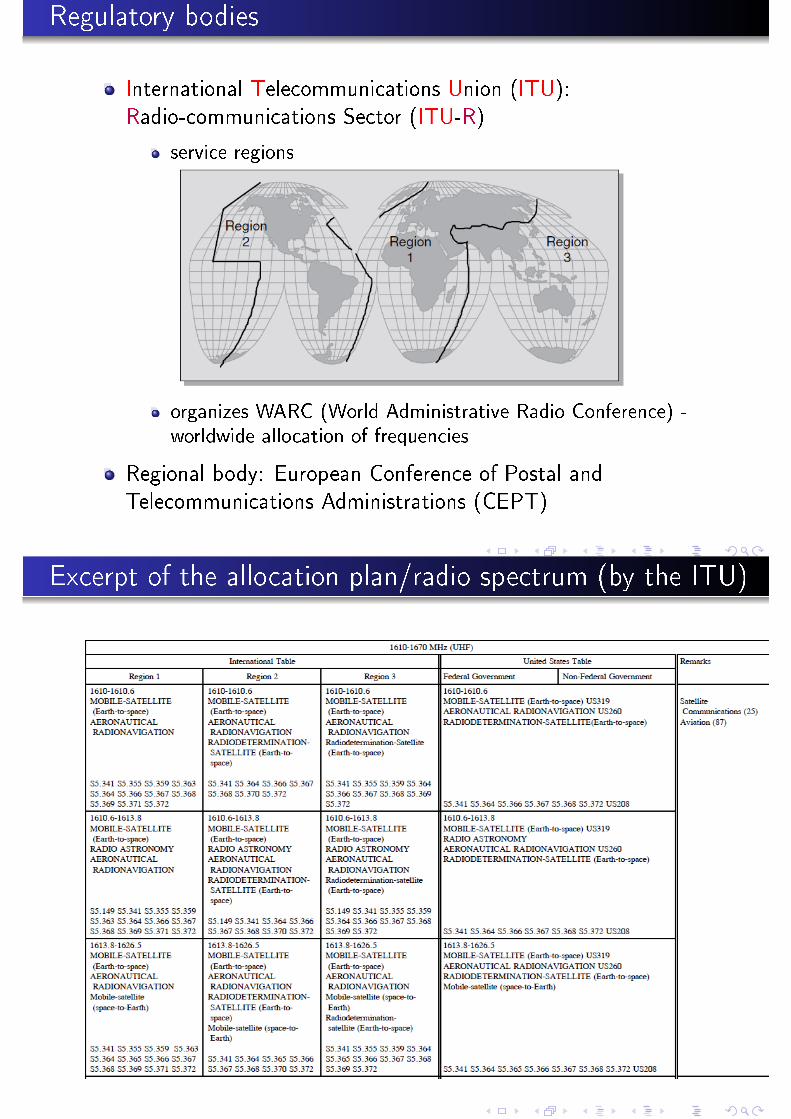
Regulatory bodies

International Telecommunications Union (ITU):Radio-communications Sector (ITU-R)

service regions

organizes WARC (World Administrative Radio Conference) -worldwide allocation of frequencies

Regional body: European Conference of Postal andTelecommunications Administrations (CEPT)

Excerpt of the allocation plan/radio spectrum (by the ITU)

Frequency allocations [2]

Radio-communications service Typical up/down link Terminology

Fixed satellite service (FSS) 6/4 [GHz] C band

8/7 [GHz] X band

14/12.1 [GHz] Ku band

30/20 [GHz] Ka band

50/40 [GHz] V band

Mobile satellite service (MSS) 1.6/1.5 [GHz] L band

30/20 [GHz] Ka band

Broadcasting satellite service (BSS) 2/2.2 [GHz] S band

12 [GHz] Ku band

2.6/2.5 [GHz] S band

Note that frequencies for down links are usually lower than for up links:this is because attenuation increases with the frequency.

The use of higher frequencies allows larger bandwidths, better trackingcapability and minimizes ionospheric e�ects. But it also requires greaterpointing accuracy

Frequency allocations [2]

Radio-communications service Typical up/down link Terminology

Fixed satellite service (FSS) 6/4 [GHz] C band

8/7 [GHz] X band

14/12.1 [GHz] Ku band

30/20 [GHz] Ka band

50/40 [GHz] V band

Mobile satellite service (MSS) 1.6/1.5 [GHz] L band

30/20 [GHz] Ka band

Broadcasting satellite service (BSS) 2/2.2 [GHz] S band

12 [GHz] Ku band

2.6/2.5 [GHz] S band

Note that frequencies for down links are usually lower than for up links:this is because attenuation increases with the frequency.

The use of higher frequencies allows larger bandwidths, better trackingcapability and minimizes ionospheric e�ects. But it also requires greaterpointing accuracy

Orbits

Engineering considerations:

distance between user and satellite.

delay (increases with the distance)attenuation of the signal (increases with the distance)

relative position of the user/satellite pair


Engineering


Outline




Modulation

Multiplexing





3 Engineering

Noise

Link budget



Engineering



dPR

PT

Important issues:

channel characteristics

attenuation (distance)atmospheric e�ects

wave polarizationrain mitigation

antenna design

power budget (related to the Signal to Noise ratio)


Inverse square law of radiation

The power �ux density (or power density) S , over the surface of asphere of radius ra from the point P , is given by (Poynting vector)

Sa =Pt4πr2a

[W

m2

](12)

E�ective Isotropic Radiated Power [EIRP]

De�nition (EIRP)

The E�ective Isotropic Radiated Power (EIRP) of a transmitter is thepower that the transmitter appears to have if the transmitter werean isotropic radiator (if the antenna radiated equally in alldirections).

From the receiver's point of view,

Pt = PTGT (13)

where:

Pt is the power of a imaginary isotropic antenna.

PT is the transmitter power and GT is its gain (in thatdirection).

If the cable losses can be neglected, then EIRP= PTGT .

E�ective area

De�nition (E�ective area)

The e�ective area of an antenna is the ratio of the available powerto the power �ux density (Poynting vector):

Ae� ,R =P

Se�(14)

Theorem

The e�ective area of an antenna is related to its gain by thefollowing formula

Ae� ,R = GRλ 2

4π(15)

Friis's relationship

We have

dPR

PT

PR = Se� ,RAe� ,R

=

(PTGT

4πd2

)Ae� ,R =

(PTGT

4πd2

)(λ 2

4π

)GR = PTGTGR

(λ

4πd

)2

Free space path loss Friis's relationship

LFS =(

λ4πd

)2ε = PT

PR=(4πd

λ)2 1

GTGR

Decibel as a common power unit

x ↔ 10 log10(x) [dB] (16)

P [dBm] = 10 log10P [mW]

1 [mW](17)

x [W] 10 log10(x) [dBW]

1 [W] 0 [dBW]

2 [W] 3 [dBW]

0,5 [W] −3 [dBW]

5 [W] 7 [dBW]

10n [W] 10×n [dBW]

Orders of magnitude in satellite communications:

transmitter power: 100 [W]≡ 20 [dB]

received power: 100 [pW] = 100×10−12[W]≡−100 [dB]

Free space losses

Are high frequencies less adequate?

In [dB], Friis's relationship becomes

ε = 32.5+20 log f[MHz]+20 logd[km]−GT [dB]−GR [dB]

The attenuation (loss) increases with f . So ?!

Remember that

Ae� = Gλ 2

4π(18)

So,

ε =

(4πd

λ

)2 1

GTGR=

(4πd

λ

)2 λ 2

4πAT

λ 2

4πAR(19)

=λ 2d2

ATAR=

c2d2

f 2ATAR(20)

It all depends on the antenna gains!

Are high frequencies less adequate?

In [dB], Friis's relationship becomes

ε = 32.5+20 log f[MHz]+20 logd[km]−GT [dB]−GR [dB]

The attenuation (loss) increases with f . So ?!

Remember that

Ae� = Gλ 2

4π(18)

So,

ε =

(4πd

λ

)2 1

GTGR=

(4πd

λ

)2 λ 2

4πAT

λ 2

4πAR(19)

=λ 2d2

ATAR=

c2d2

f 2ATAR(20)

It all depends on the antenna gains!

Practical case: VSAT in the Ku-band [1]

Antenna gains: 48.93 [dB]

The free space path loss is, in [dB],

LFS = 32.5+20 log f[MHz]+20 logd[km] = 205.1 [dB]

The received power is, in [dB],

PR = PT +GT +GR −LFS (21)

= 10+48.93+48.93−205.1=−97.24 [dB] (22)

In [W], the received power is

PR = 10−97.2410 = 1.89×10−10 [W] = 189 [pW] (23)


Engineering


Outline




Modulation

Multiplexing





3 Engineering

Noise

Link budget



Engineering


Terrestrial antennas


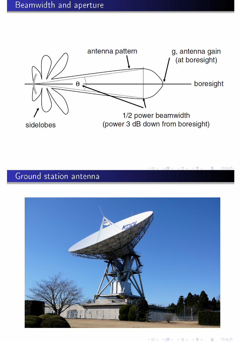
Beamwidth and aperture

Ground station antenna

Parabolic (dish) antenna

Radiation pattern

Deployable antenna

Horn antenna and waveguide feed

Yagi antenna

Patch array antenna

Phased array antenna

Radiowave propagation mechanisms

+ Doppler e�ect

Earth atmosphere absorption

Expressed in terms of the wavelength:λ [m] = cf= 3×108 [m/s]

f [Hz]

Attenuation due to atmospheric gases

Zenith attenuation due to atmospheric gases (source: ITU-R P.676-6)

[O2 and H20 are the main contributors]

Rain attenuation

Total path rain attenuation as a function of frequency and elevation angle.

Location: Washington, DC, Link Availability: 99%

Cloud attenuation

Cloud attenuation as a function of frequency, for elevation angles from 5 to 30°

Total attenuation

The ITU recommends that all tropospheric contributions to signalattenuation are combined as follows:

AT (p) = AG +

√(AR(p)+Ac(p))

2+As(p) (24)

where:

AT (p) is the total attenuation for a given probability

AG (p) is the attenuation due to water vapor and oxygen

AR(p) is the attenuation due to rain

Ac(p) is the attenuation due to clouds

As(p) is the attenuation due to scintillation (rapid �uctuationsattributed to irregularities in the tropospheric refractive index)

Service Level Agreement (SLA)

Customers ask for a guaranteed level of quality: this leads to aService Level Agreement (SLA) with the satellite operator.In engineering terms: introduction of power margins!


Engineering

NoiseLink budget

Outline




Modulation

Multiplexing





3 Engineering

Noise

Link budget



Engineering

NoiseLink budget

Noise

Theorem (Nyquist's formula for a one-port noise generator)

The available power from a thermal source in a bandwidth of W is

PN = kBT W (25)

where

kB = 1,38×10−23 [J/K ] is the constant of Boltzmann(=198 [dBm/K/Hz] ==228.6 [dBW/K/Hz]),

T is the equivalent noise temperature of the noise source

W is the bandwidth of the system

Thermal noise is one the main sources of noise in a satellite → putelectronics in the cold zone of a satellite


Noise in two-port circuits

De�nitions

Noise Factor (F): [provided by the manufacturer]

F=

(SN

)in(

SN

)out

> 1 (26)

Noise Figure (NF):NF=10 log10F (27)

E�ective noise temperature Te (T0 = 290 [K ]):

Te = T0(F −1) (28)

Noise factor of a two-port cascade

γaN1(f )

(F01−1)γaN1(f )

(F02−1)γaN1(f )

G1F01γaN1(f )

G2G1

F02F01

Figure : Cascading two-port elements.

For a two-port network with n stages,

F0 = F01+F02−1

G1+F03−1

G1G2+ · · ·= F01+

n

∑i=2

F0i −1

∏i−1j=1Gj

(29)

Likewise,

Te = Te1+Te2

G1+

Te3

G1G2+ · · ·= Te1+

n

∑i=2

Tei

∏i−1j=1Gj

(30)

Receiver front end I

Figure : Block diagram of a typical receiver.

Receiver front end II

Rule of thumb: highest gain (G1) and best noise �gure (F01) �rst.

Then

F0 = F01+F02−1

G1+F03−1

G1G2+ · · · ' F01+

F02−1

G 1(31)

Te = Te1+Te2

G1+

Te3

G1G2+ · · · ' Te1+

Te2

G1(32)

Example of the calculation of a noise budget [1]

Low Noise Ampli�er: TLA = 290× (10410 −1) = 438 [K ]

Line. For a passive two-part, the noise factor is theattenuation F0 = A.

TLine = 290× (10310 −1) = 289 [K ],

GLine =1

2

The e�ective noise temperature, including the antenna noise, is

Te = tA+Te1+Te2

G1+

Te3

G1G2+ · · · (33)

= 60+438︸︷︷︸498

+289

1000+

2610

1000× 12

+ · · ·= 509.3 [K ] (34)

Typical values for the increase in antenna temperature dueto rain [1]


Engineering

NoiseLink budget

Outline




Modulation

Multiplexing





3 Engineering

Noise

Link budget



Engineering

NoiseLink budget

Example of parameter values for a communicationsatellite [1]

Parameter uplink downlink

Frequency 14.1 [GHz] 12.1 [GHz]

Bandwidth 30 [MHz] 30 [MHz]

Transmitter power 100−1000 [W] 20−200 [W]

Transmitter antenna gain 54 [dBi ] 36.9 [dBi ]

Receiver antenna gain 37.9 [dBi ] 52.6 [dBi ]

Receiver noise �gure 8 [dB] 3 [dB]

Receiver antenna temperature 290 [K ] 50 [K ]

Free space path loss (30° elevation) 207.2 [dB] 205.8 [dB]


Clear sky down link performance [2]


Engineering

NoiseLink budget

For further reading

L. Ippolito.Satellite Communications Systems Engineering: AtmosphericE�ects, Satellite Link Design and System Performance. Wiley,2008.

G. Maral, M. Bousquet.Satellite Communications Systems: Systems, Techniques andTechnology. Wiley, 2002.

J. Gibsons.The Communications Handbook. CRC Press, 1997.

Wikipedia.http://wikipedia.org


Documents

Satellite Communications - LTAS-SDRG Communications ... Link budget Marc Van ... Main type s of satellite ! di erent types of information Astronomical satellites: