Embed Size (px)
Citation preview
NWP SAF Second Analysis of the NWP SAF AMV Monitoring
Doc ID : NWPSAF-MO-TR-020 Version : 1.3 Date : 13/12/05
1
NWP SAF
Satellite Application Facility for Numerical Weather Prediction Document NWPSAF-MO-TR-020
Version 1.3
13/12/05
Second Analysis of the data displayed on the NWP SAF AMV monitoring website
Mary Forsythe and Marie Doutriaux-Boucher Met Office, UK
NWP SAF Second Analysis of the NWP SAF AMV Monitoring
Doc ID : NWPSAF-MO-TR-020 Version : 1.3 Date : 13/12/05
2
Second Analysis of the data displayed on the NWP SAF AMV monitoring website
Mary Forsythe, Marie Doutriaux-Boucher
Met Office, UK This documentation was developed within the context of the EUMETSAT Satellite Application Facility on Numerical Weather Prediction (NWP SAF), under the Cooperation Agreement dated 16 December, 2003, between EUMETSAT and the Met Office, UK, by one or more partners within the NWP SAF. The partners in the NWP SAF are the Met Office, ECMWF, KNMI and Météo France. Copyright 2005, EUMETSAT, All Rights Reserved.
Change record Version Date Author / changed by Remarks
1.1 07/11/05 Mary Forsythe Almost first draft 1.2 25/11/05 Mary Forsythe First complete draft. Modified after comments from Bryan
Conway and Marie Doutriaux-Boucher 1.3 13/12/05 Mary Forsythe Modified after comments from Roger Saunders, John Eyre,
Jörgen Gustafsson, Jo Schmetz, Régis Borde, Sean Milton and Niels Bormann.
NWP SAF Second Analysis of the NWP SAF AMV Monitoring
Doc ID : NWPSAF-MO-TR-020 Version : 1.3 Date : 13/12/05
3
Contents Page
1. Introduction . . . . . . . . . . . . . . . . . . . . . . . . . . . . . . . . . . . . . . . . . . . . . . . . . . . . . . . . . . . . . . . . 5 2. Error Sources . . . . . . . . . . . . . . . . . . . . . . . . . . . . . . . . . . . . . . . . . . . . . . . . . . . . . . . . . . . . . . 5 2.1. NWP model error . . . . . . . . . . . . . . . . . . . . . . . . . . . . . . . . . . . . . . . . . . . . . . . . . . . . . . . . . . . 5 2.2. AMV error . . . . . . . . . . . . . . . . . . . . . . . . . . . . . . . . . . . . . . . . . . . . . . . . . . . . . . . . . . . . . . . . 6 2.2.1. Introduction . . . . . . . . . . . . . . . . . . . . . . . . . . . . . . . . . . . . . . . . . . . . . . . . . . . . . . . . . . . 6 2.2.2. AMV as a representative of the local wind field . . . . . . . . . . . . . . . . . . . . . . . . . . . . . . . . 6 2.2.3. Vector error . . . . . . . . . . . . . . . . . . . . . . . . . . . . . . . . . . . . . . . . . . . . . . . . . . . . . . . . . . . 7 2.2.4. Height error . . . . . . . . . . . . . . . . . . . . . . . . . . . . . . . . . . . . . . . . . . . . . . . . . . . . . . . . . . . 8 2.2.5. Post-processing . . . . . . . . . . . . . . . . . . . . . . . . . . . . . . . . . . . . . . . . . . . . . . . . . . . . . . . . 11 3. The NWP SAF AMV monitoring . . . . . . . . . . . . . . . . . . . . . . . . . . . . . . . . . . . . . . . . . . . . . . . . 12 3.1. Introduction . . . . . . . . . . . . . . . . . . . . . . . . . . . . . . . . . . . . . . . . . . . . . . . . . . . . . . . . . . . . . . . 12 3.2. Recent developments to the NWP SAF AMV monitoring . . . . . . . . . . . . . . . . . . . . . . . . . . . . . 12 3.3. Types of plots . . . . . . . . . . . . . . . . . . . . . . . . . . . . . . . . . . . . . . . . . . . . . . . . . . . . . . . . . . . . . . 13 4. Features observed in the O-B statistics plots . . . . . . . . . . . . . . . . . . . . . . . . . . . . . . . . . . . . 13 4.1. Interpreting the plots . . . . . . . . . . . . . . . . . . . . . . . . . . . . . . . . . . . . . . . . . . . . . . . . . . . . . . . . 13 4.2. General observations from the plots . . . . . . . . . . . . . . . . . . . . . . . . . . . . . . . . . . . . . . . . . . . . 13 4.3. Specific features of interest . . . . . . . . . . . . . . . . . . . . . . . . . . . . . . . . . . . . . . . . . . . . . . . . . . . 15 4.3.1. Introduction . . . . . . . . . . . . . . . . . . . . . . . . . . . . . . . . . . . . . . . . . . . . . . . . . . . . . . . . . . . . 15 4.3.2. Low level (below 700 hPa) . . . . . . . . . . . . . . . . . . . . . . . . . . . . . . . . . . . . . . . . . . . . . . . . 15 Feature 2.1. Fast bias at low wind speeds . . . . . . . . . . . . . . . . . . . . . . . . . . . . . . . . . . . . . 16 Feature 2.2. Indian Ocean . . . . . . . . . . . . . . . . . . . . . . . . . . . . . . . . . . . . . . . . . . . . . . . . . 16 Feature 2.3. Eastern USA winter low level slow speed bias . . . . . . . . . . . . . . . . . . . . . . . 18 Feature 2.4. Low level fast bias from 40S to 60S for Meteosat satellites . . . . . . . . . . . . . 19 Feature 2.5. Trade wind fast bias . . . . . . . . . . . . . . . . . . . . . . . . . . . . . . . . . . . . . . . . . . . 20 Feature 2.6. Fast bias over Sahara desert in summer . . . . . . . . . . . . . . . . . . . . . . . . . . . . 21 Feature 2.7. Fast bias at low level below high level jets . . . . . . . . . . . . . . . . . . . . . . . . . . 22 4.3.3. Mid level (400-700 hPa) . . . . . . . . . . . . . . . . . . . . . . . . . . . . . . . . . . . . . . . . . . . . . . . . . 23 Feature 2.8. Fast bias in the tropics . . . . . . . . . . . . . . . . . . . . . . . . . . . . . . . . . . . . . . . . . . 24 Feature 2.9. Slow bias in the extratropics . . . . . . . . . . . . . . . . . . . . . . . . . . . . . . . . . . . . . 26 4.3.4. High level (above 400 hPa) . . . . . . . . . . . . . . . . . . . . . . . . . . . . . . . . . . . . . . . . . . . . . . . 27 Feature 2.10. Jet region slow bias . . . . . . . . . . . . . . . . . . . . . . . . . . . . . . . . . . . . . . . . . . . 28 Feature 2.11. NESDIS over-correction of slow bias in jets . . . . . . . . . . . . . . . . . . . . . . . . 30 Feature 2.12. Indian Ocean fast bias . . . . . . . . . . . . . . . . . . . . . . . . . . . . . . . . . . . . . . . . . 31 Feature 2.13. Tropics fast bias . . . . . . . . . . . . . . . . . . . . . . . . . . . . . . . . . . . . . . . . . . . . . . 32 Feature 2.14. Very high level (above 180 hPa) fast bias . . . . . . . . . . . . . . . . . . . . . . . . . . 33 Feature 2.15. Differences between channels . . . . . . . . . . . . . . . . . . . . . . . . . . . . . . . . . . . 33 4.3.5. Polar winds . . . . . . . . . . . . . . . . . . . . . . . . . . . . . . . . . . . . . . . . . . . . . . . . . . . . . . . . . . . . 36 Feature 2.16. Number of MODIS IR winds . . . . . . . . . . . . . . . . . . . . . . . . . . . . . . . . . . . . . 36 Feature 2.17. CIMSS MODIS mid level fast winds . . . . . . . . . . . . . . . . . . . . . . . . . . . . . . . 36 Feature 2.18. CIMSS MODIS slow winds . . . . . . . . . . . . . . . . . . . . . . . . . . . . . . . . . . . . . 37 Feature 2.19. High level fast speed bias in edited MODIS data . . . . . . . . . . . . . . . . . . . . . 37 Feature 2.20. Low level slow speed bias in NESDIS MODIS IR data . . . . . . . . . . . . . . . . 38 5. Approach in NWP . . . . . . . . . . . . . . . . . . . . . . . . . . . . . . . . . . . . . . . . . . . . . . . . . . . . . . . . . . . 38 5.1. Blacklisting . . . . . . . . . . . . . . . . . . . . . . . . . . . . . . . . . . . . . . . . . . . . . . . . . . . . . . . . . . . . . . . 38 5.2. Quality Indicator thresholds . . . . . . . . . . . . . . . . . . . . . . . . . . . . . . . . . . . . . . . . . . . . . . . . . . . 38 5.3. Bias correction . . . . . . . . . . . . . . . . . . . . . . . . . . . . . . . . . . . . . . . . . . . . . . . . . . . . . . . . . . . . 40 5.4. Thinning . . . . . . . . . . . . . . . . . . . . . . . . . . . . . . . . . . . . . . . . . . . . . . . . . . . . . . . . . . . . . . . . . . 40 5.5. Observation error setting . . . . . . . . . . . . . . . . . . . . . . . . . . . . . . . . . . . . . . . . . . . . . . . . . . . . . 40 5.6. Background check . . . . . . . . . . . . . . . . . . . . . . . . . . . . . . . . . . . . . . . . . . . . . . . . . . . . . . . . . . 40 5.7. Observation operator . . . . . . . . . . . . . . . . . . . . . . . . . . . . . . . . . . . . . . . . . . . . . . . . . . . . . . . . 40
NWP SAF Second Analysis of the NWP SAF AMV Monitoring
Doc ID : NWPSAF-MO-TR-020 Version : 1.3 Date : 13/12/05
4
5.8. Variational quality control . . . . . . . . . . . . . . . . . . . . . . . . . . . . . . . . . . . . . . . . . . . . . . . . . . . . 40 6. Conclusions . . . . . . . . . . . . . . . . . . . . . . . . . . . . . . . . . . . . . . . . . . . . . . . . . . . . . . . . . . . . . . . 41 7. Revised action list . . . . . . . . . . . . . . . . . . . . . . . . . . . . . . . . . . . . . . . . . . . . . . . . . . . . . . . . . . 41 7.1. Discrepancies between contributors . . . . . . . . . . . . . . . . . . . . . . . . . . . . . . . . . . . . . . . . . . . . 42 7.2. Improvements to site design . . . . . . . . . . . . . . . . . . . . . . . . . . . . . . . . . . . . . . . . . . . . . . . . . . 42 7.3. Development of plots . . . . . . . . . . . . . . . . . . . . . . . . . . . . . . . . . . . . . . . . . . . . . . . . . . . . . . . 42 7.4. Analysis of results . . . . . . . . . . . . . . . . . . . . . . . . . . . . . . . . . . . . . . . . . . . . . . . . . . . . . . . . . . 42 7.5. Follow up investigations . . . . . . . . . . . . . . . . . . . . . . . . . . . . . . . . . . . . . . . . . . . . . . . . . . . . . . 43 8. Further recommendations . . . . . . . . . . . . . . . . . . . . . . . . . . . . . . . . . . . . . . . . . . . . . . . . . . . . . 43 8.1. Recommendations for producers . . . . . . . . . . . . . . . . . . . . . . . . . . . . . . . . . . . . . . . . . . . . . . . 43 8.2. Recommendations for users . . . . . . . . . . . . . . . . . . . . . . . . . . . . . . . . . . . . . . . . . . . . . . . . . . . 44 8. Acknowledgements . . . . . . . . . . . . . . . . . . . . . . . . . . . . . . . . . . . . . . . . . . . . . . . . . . . . . . . . . 45 9. References . . . . . . . . . . . . . . . . . . . . . . . . . . . . . . . . . . . . . . . . . . . . . . . . . . . . . . . . . . . . . . . . . 45
NWP SAF Second Analysis of the NWP SAF AMV Monitoring
Doc ID : NWPSAF-MO-TR-020 Version : 1.3 Date : 13/12/05
5
1. Introduction There is general agreement within the Atmospheric Motion Vector (AMV) community that we are not yet seeing full benefit from the AMV data in Numerical Weather Prediction (NWP). One of the difficulties is that the AMV errors are hard to characterise and are typically non-Gaussian and correlated. To gain more benefit in NWP it is essential to improve our understanding of the errors. This may highlight areas for potential improvement in the wind derivation and height assignment, but will also provide more guidance for quality control and observation errors in NWP. Why is this important for NWP? Currently AMVs are the only wind observation with good global coverage. They are the only source of wind information in the polar regions and over much of the global oceans. There are regions, in particular the tropics, where information on the wind field cannot be indirectly inferred from the mass field. It is in these regions where AMVs are seen to have most impact (e.g. Sarrazin & Zaitseza, 2004; von Bremen et al., 2004). In order to maximise the benefit from AMVs in NWP it is important that we can identify and remove or down weight bad observations. To be able to do this we need to understand the sources of error and have access to quality indicators that reflect these errors effectively. The NWP SAF AMV monitoring report is a useful resource for investigating AMV errors. Its purpose is to provide comparable AMV monitoring output from different NWP centres in order to help identify and partition error contributions from AMVs and the NWP models. The report is freely available at http://www.metoffice.gov.uk/research/interproj/nwpsaf/satwind_report/. The site provides more than three years of monthly observation-background statistics plots from ECMWF and the Met Office. Recently, several changes have been made to the site to allow easier plot comparison, to include new AMVs and to provide new types of statistical plots. Other information is also available from this site including links to summaries of AMV work and links to other AMV monitoring sites. The site is intended to stimulate thought and discussion and eventually to lead to improved production, as well as improvements in NWP models and assimilation procedures. The purpose of this paper is to identify and describe some of the discrepancies between AMVs and model backgrounds that are evident in the NWP SAF AMV statistics plots. Further investigations have been carried out to look at some of the features in more detail. The paper concludes with a list of recommendations for the contributors to the NWP SAF AMV monitoring, for the AMV producers and for other users. The actions include items to improve the usefulness of the site, ideas for future investigations and suggestions for improvements to the AMV product. Increased discussion within the AMV community is encouraged to pursue these issues further. 2. Error sources Errors exist in both the NWP model backgrounds and the AMV data; neither can be assumed to be the truth. Before, discussing the results of the analysis of the NWP SAF AMV plots, a summary is provided of some of the known sources of error in the NWP models and the AMVs, which may contribute to some of the differences seen in the observation-background (O-B) plots. 2.1. NWP model error The accuracy of the NWP model short-term forecasts is dependent on both the accuracy of the initial conditions (determined by the available observations and the assimilation scheme) and the accuracy of the forecast model. The accuracy of the initial conditions will depend on the distribution of observations (less well constrained in data poor areas), the accuracy of those observations and how the information from the observations are used to correct the state of the atmosphere. In the data assimilation scheme, the information in the observations is spread out horizontally and vertically, with no direct allowance for presence of sharp gradients at frontal boundaries etc (although 4D-Var does this implicitly to some extent). One effect of this is the tendency to produce smoother analyses, with less tightly constrained fronts and jets. Another limitation is the resolution of the analysis and forecast models. A general rule of thumb is that models can only simulate phenomena that have spatial scales of at least 4x the distance between grid points. For the Met Office global model, the data assimilation is run at N108 (equates to a grid spacing of 120 km at the latitude of the UK), so only features with scales of >~500 km will be represented. The forecast model is also affected by the limited horizontal and vertical resolution. A major constraint of forecast models is the influence of unresolved scales. Some smaller scale processes, such as convection and turbulence, cannot be captured directly and must be parameterized (necessarily an imperfect process). Similarly, model
NWP SAF Second Analysis of the NWP SAF AMV Monitoring
Doc ID : NWPSAF-MO-TR-020 Version : 1.3 Date : 13/12/05
6
resolution limits the representation of the lower boundary conditions (topography and coastlines), and thus models may fail to capture some topographic or coastline related effects e.g. sea breezes and valley fog. A thorough analysis of the NWP model short-term forecast error is a whole study in itself and only a short note is included here. As with observations, model forecasts can be verified by comparing to model analyses or observations. In comparisons to analyses, it is evident that some errors spin up quite quickly and can affect even the short-range forecasts (including the 6-hour forecasts used in the NWP SAF AMV monitoring), though the errors are normally much smaller than those seen at longer range. Seasonal root mean square difference plots for Met Office 24 hour forecasts compared with analyses show the biggest values in the jet regions and the differences are greatest in the winter hemisphere (up to 8 m/s). The mean wind u-component differences (systematic differences) are greatest in the lower latitudes (up to 4 m/s), primarily in the Pacific and Indian Oceans and over West Africa, and are associated with errors in the precipitation forecasts (Milton et al., 2003). An example for the summer months is the tendency to have too strong low level easterlies over Indonesia and the equatorial Indian Ocean and too strong high level westerlies along the equatorward side of the sub-tropical jet where it crosses the Indian Ocean. The wind errors are associated with a greater low level convergence – high level divergence in the Indian Ocean in the 24 hour forecasts compared to the verifying analyses. The errors are thought to be primarily linked to inaccuracies in the representation of the convection and possible topographic influence on the flow (for example over Indonesia and the Himalayas). 2.2. AMV error 2.2.1. Introduction Before discussing the sources of error in the AMV data, it is useful to summarise the main steps in the AMV derivation. There are some differences from producer to producer, but essentially all AMVs are generated by tracking clouds or areas of water vapour in consecutive satellite images. The derivation is composed of several steps:
1. Correct and rectify the raw data 2. Locate a suitable tracer within the image 3. Perform a cross-correlation to locate the same feature in an earlier or later image. 4. Calculate the vector from the displacement in tracer location 5. Assign a height to the vector 6. Perform some quality control
The final AMV is an average of two or three component vectors calculated from a sequence of three or four images. For further information on AMV derivation, see Schmetz et al. (1993) and Nieman et al. (1997). There are various sources of error in the AMV data that can be introduced in the tracking and height assignment. Sometimes all AMVs in a particular area will be affected by the same errors and similar errors can persist to the next derivation cycle. This tendency means that the AMV data has temporally and spatially correlated errors. This is not allowed for directly by the NWP assimilation and so precautions need to be taken (currently the data is thinned). In addition to the error in the AMV derivation, there is also the consideration of how well the final AMV represents the wind field at a specific location, height and time. As Schmetz & Nuret (1989) stated the AMVs could only give an unbiased estimate of the winds if clouds were conservative tracers randomly distributed within and floating with the airflow. This is clearly not the case; clouds are not randomly arranged, but associated with specific conditions (ascending air masses), some clouds do not move with the wind while others follow the wind at a level lower than the cloud top. Additionally the AMVs represent the movement of a layer of the atmosphere and are a spatial and temporal average. All these things should be understood and considered when deciding how to use them optimally in NWP. The following sections detail some of the sources of error in the AMV data. 2.2.2. AMV as a representative of the local wind field 1. Clouds do not always behave as passive tracers (e.g. Holmlund & Schmetz, 1990). They often change shape with time, for example, expanding outwards in regions of upper level tropical divergence. The
NWP SAF Second Analysis of the NWP SAF AMV Monitoring
Doc ID : NWPSAF-MO-TR-020 Version : 1.3 Date : 13/12/05
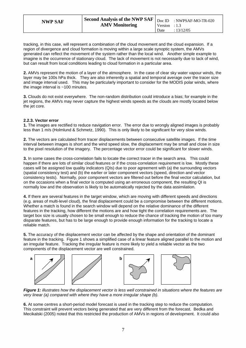
tracking, in this case, will represent a combination of the cloud movement and the cloud expansion. If a region of divergence and cloud formation is moving within a large scale synoptic system, the AMVs generated can reflect the movement of the system rather than the local wind. Another simple example to imagine is the occurrence of stationary cloud. The lack of movement is not necessarily due to lack of wind, but can result from local conditions leading to cloud formation in a particular area. 2. AMVs represent the motion of a layer of the atmosphere. In the case of clear sky water vapour winds, the layer may be 100s hPa thick. They are also inherently a spatial and temporal average over the tracer size and image interval used. This may be particularly important to consider for the MODIS polar winds, where the image interval is ~100 minutes. 3. Clouds do not exist everywhere. The non-random distribution could introduce a bias; for example in the jet regions, the AMVs may never capture the highest winds speeds as the clouds are mostly located below the jet core. 2.2.3. Vector error 1. The images are rectified to reduce navigation error. The error due to wrongly aligned images is probably less than 1 m/s (Holmlund & Schmetz, 1990). This is only likely to be significant for very slow winds. 2. The vectors are calculated from tracer displacements between consecutive satellite images. If the time interval between images is short and the wind speed slow, the displacement may be small and close in size to the pixel resolution of the imagery. The percentage vector error could be significant for slower winds. 3. In some cases the cross-correlation fails to locate the correct tracer in the search area. This could happen if there are lots of similar cloud features or if the cross-correlation requirement is low. Mostly these cases will be assigned low quality indicators (QIs) due to poor agreement with (a) the surrounding vectors (spatial consistency test) and (b) the earlier or later component vectors (speed, direction and vector consistency tests). Normally, poor component vectors are filtered out before the final vector calculation, but on the occasions when a final vector is computed using an erroneous component, the resulting QI is normally low and the observation is likely to be automatically rejected by the data assimilation. 4. If there are several features in the target window, which are moving with different speeds and directions (e.g. areas of multi-level cloud), the final displacement could be a compromise between the different motions. Whether a match is found in the search window will depend on the relative dominance of the different features in the tracking, how different the motions are and how tight the correlation requirements are. The target box size is usually chosen to be small enough to reduce the chance of tracking the motion of too many disparate features, but has to be large enough to provide enough information for the tracking to locate a reliable match. 5. The accuracy of the displacement vector can be affected by the shape and orientation of the dominant feature in the tracking. Figure 1 shows a simplified case of a linear feature aligned parallel to the motion and an irregular feature. Tracking the irregular feature is more likely to yield a reliable vector as the two components of the displacement vector are well constrained.
b
Figve 6. ThMe
a
7
ure 1: illustrates how the displacement vector is less well constrained in situations where the features are
ry linear (a) compared with where they have a more irregular shape (b).
At some centres a short-period model forecast is used in the tracking step to reduce the computation. is constraint will prevent vectors being generated that are very different from the forecast. Bedka and cikalski (2005) noted that this restricted the production of AMVs in regions of development. It could also
NWP SAF Second Analysis of the NWP SAF AMV Monitoring
Doc ID : NWPSAF-MO-TR-020 Version : 1.3 Date : 13/12/05
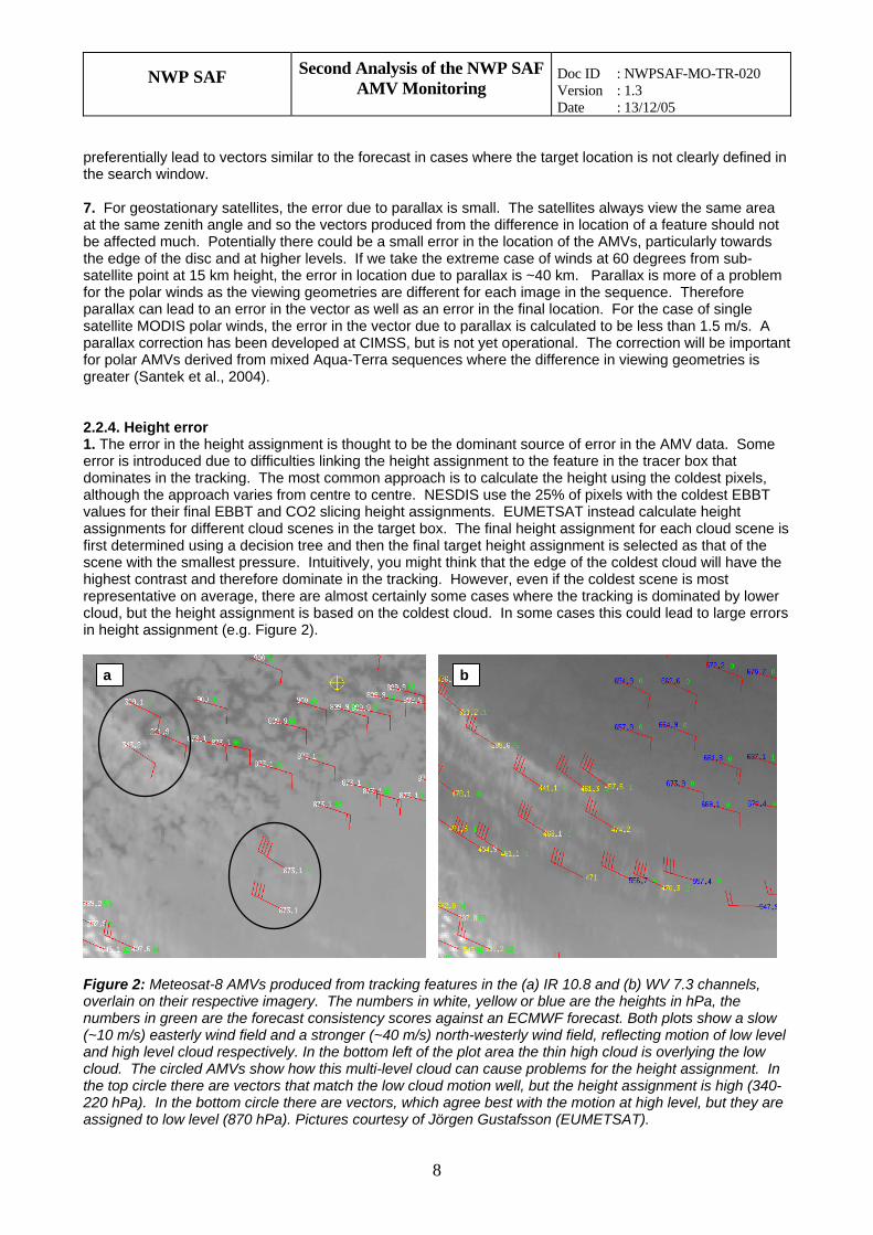
preferentially lead to vectors similar to the forecast in cases where the target location is not clearly defined in the search window. 7. For geostationary satellites, the error due to parallax is small. The satellites always view the same area at the same zenith angle and so the vectors produced from the difference in location of a feature should not be affected much. Potentially there could be a small error in the location of the AMVs, particularly towards the edge of the disc and at higher levels. If we take the extreme case of winds at 60 degrees from sub-satellite point at 15 km height, the error in location due to parallax is ~40 km. Parallax is more of a problem for the polar winds as the viewing geometries are different for each image in the sequence. Therefore parallax can lead to an error in the vector as well as an error in the final location. For the case of single satellite MODIS polar winds, the error in the vector due to parallax is calculated to be less than 1.5 m/s. A parallax correction has been developed at CIMSS, but is not yet operational. The correction will be important for polar AMVs derived from mixed Aqua-Terra sequences where the difference in viewing geometries is greater (Santek et al., 2004). 2.2.4. Height error 1. The error in the height assignment is thought to be the dominant source of error in the AMV data. Some error is introduced due to difficulties linking the height assignment to the feature in the tracer box that dominates in the tracking. The most common approach is to calculate the height using the coldest pixels, although the approach varies from centre to centre. NESDIS use the 25% of pixels with the coldest EBBT values for their final EBBT and CO2 slicing height assignments. EUMETSAT instead calculate height assignments for different cloud scenes in the target box. The final height assignment for each cloud scene is first determined using a decision tree and then the final target height assignment is selected as that of the scene with the smallest pressure. Intuitively, you might think that the edge of the coldest cloud will have the highest contrast and therefore dominate in the tracking. However, even if the coldest scene is most representative on average, there are almost certainly some cases where the tracking is dominated by lower cloud, but the height assignment is based on the coldest cloud. In some cases this could lead to large errors in height assignment (e.g. Figure 2).
Figovnu(~1anclothe22as
a
8
ure 2: Meteosat-8 AMVs produced from tracking featuerlain on their respective imagery. The numbers in whimbers in green are the forecast consistency scores aga0 m/s) easterly wind field and a stronger (~40 m/s) nor
d high level cloud respectively. In the bottom left of the ud. The circled AMVs show how this multi-level cloud top circle there are vectors that match the low cloud m
0 hPa). In the bottom circle there are vectors, which agsigned to low level (870 hPa). Pictures courtesy of Jörg
b
res in the (a) IR 10.8 and (b) WV 7.3 channels, te, yellow or blue are the heights in hPa, the inst an ECMWF forecast. Both plots show a slow th-westerly wind field, reflecting motion of low level plot area the thin high cloud is overlying the low can cause problems for the height assignment. In otion well, but the height assignment is high (340-ree best with the motion at high level, but they are en Gustafsson (EUMETSAT).
NWP SAF Second Analysis of the NWP SAF AMV Monitoring
Doc ID : NWPSAF-MO-TR-020 Version : 1.3 Date : 13/12/05
9
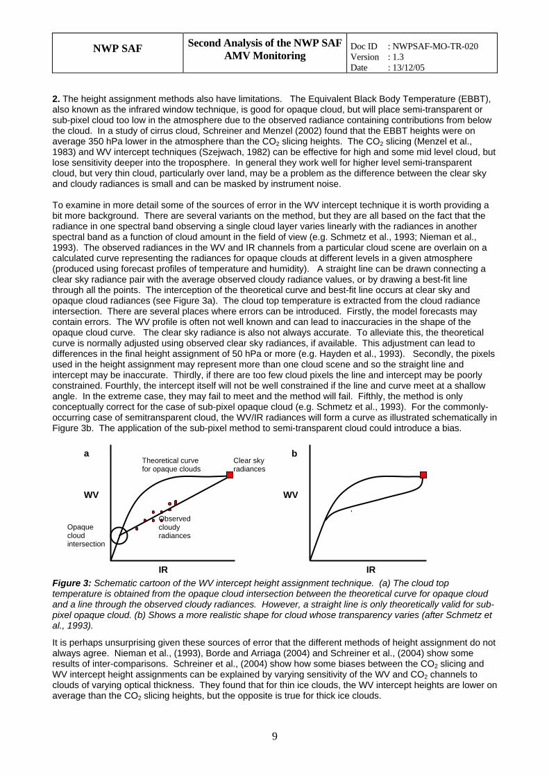
2. The height assignment methods also have limitations. The Equivalent Black Body Temperature (EBBT), also known as the infrared window technique, is good for opaque cloud, but will place semi-transparent or sub-pixel cloud too low in the atmosphere due to the observed radiance containing contributions from below the cloud. In a study of cirrus cloud, Schreiner and Menzel (2002) found that the EBBT heights were on average 350 hPa lower in the atmosphere than the CO2 slicing heights. The CO2 slicing (Menzel et al., 1983) and WV intercept techniques (Szejwach, 1982) can be effective for high and some mid level cloud, but lose sensitivity deeper into the troposphere. In general they work well for higher level semi-transparent cloud, but very thin cloud, particularly over land, may be a problem as the difference between the clear sky and cloudy radiances is small and can be masked by instrument noise. To examine in more detail some of the sources of error in the WV intercept technique it is worth providing a bit more background. There are several variants on the method, but they are all based on the fact that the radiance in one spectral band observing a single cloud layer varies linearly with the radiances in another spectral band as a function of cloud amount in the field of view (e.g. Schmetz et al., 1993; Nieman et al., 1993). The observed radiances in the WV and IR channels from a particular cloud scene are overlain on a calculated curve representing the radiances for opaque clouds at different levels in a given atmosphere (produced using forecast profiles of temperature and humidity). A straight line can be drawn connecting a clear sky radiance pair with the average observed cloudy radiance values, or by drawing a best-fit line through all the points. The interception of the theoretical curve and best-fit line occurs at clear sky and opaque cloud radiances (see Figure 3a). The cloud top temperature is extracted from the cloud radiance intersection. There are several places where errors can be introduced. Firstly, the model forecasts may contain errors. The WV profile is often not well known and can lead to inaccuracies in the shape of the opaque cloud curve. The clear sky radiance is also not always accurate. To alleviate this, the theoretical curve is normally adjusted using observed clear sky radiances, if available. This adjustment can lead to differences in the final height assignment of 50 hPa or more (e.g. Hayden et al., 1993). Secondly, the pixels used in the height assignment may represent more than one cloud scene and so the straight line and intercept may be inaccurate. Thirdly, if there are too few cloud pixels the line and intercept may be poorly constrained. Fourthly, the intercept itself will not be well constrained if the line and curve meet at a shallow angle. In the extreme case, they may fail to meet and the method will fail. Fifthly, the method is only conceptually correct for the case of sub-pixel opaque cloud (e.g. Schmetz et al., 1993). For the commonly-occurring case of semitransparent cloud, the WV/IR radiances will form a curve as illustrated schematically in Figure 3b. The application of the sub-pixel method to semi-transparent cloud could introduce a bias.
a b Theoretical curve for opaque clouds
Clear sky radiances
WV WV
Observed cloudy radiances
Opaque cloud intersection
IR IR Figure 3: Schematic cartoon of the WV intercept height assignment technique. (a) The cloud top temperature is obtained from the opaque cloud intersection between the theoretical curve for opaque cloud and a line through the observed cloudy radiances. However, a straight line is only theoretically valid for sub-pixel opaque cloud. (b) Shows a more realistic shape for cloud whose transparency varies (after Schmetz et al., 1993).
It is perhaps unsurprising given these sources of error that the different methods of height assignment do not always agree. Nieman et al., (1993), Borde and Arriaga (2004) and Schreiner et al., (2004) show some results of inter-comparisons. Schreiner et al., (2004) show how some biases between the CO2 slicing and WV intercept height assignments can be explained by varying sensitivity of the WV and CO2 channels to clouds of varying optical thickness. They found that for thin ice clouds, the WV intercept heights are lower on average than the CO2 slicing heights, but the opposite is true for thick ice clouds.
NWP SAF Second Analysis of the NWP SAF AMV Monitoring
Doc ID : NWPSAF-MO-TR-020 Version : 1.3 Date : 13/12/05
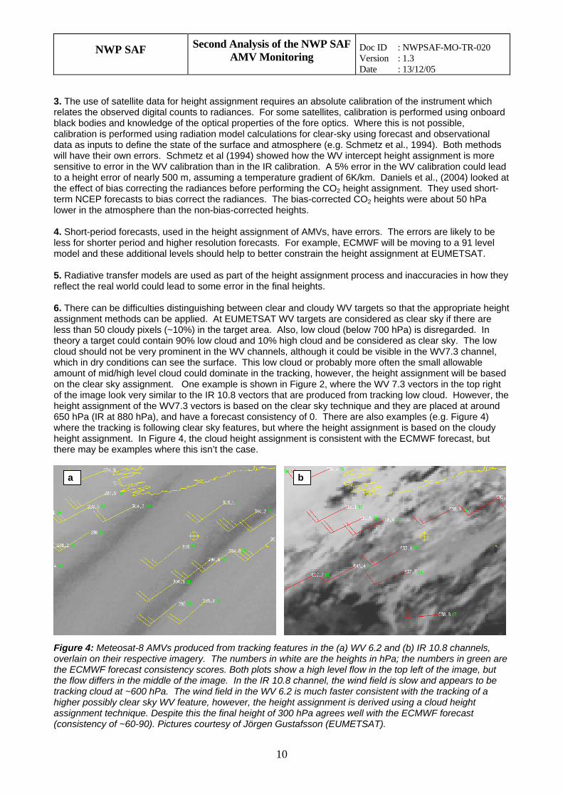
3. The use of satellite data for height assignment requires an absolute calibration of the instrument which relates the observed digital counts to radiances. For some satellites, calibration is performed using onboard black bodies and knowledge of the optical properties of the fore optics. Where this is not possible, calibration is performed using radiation model calculations for clear-sky using forecast and observational data as inputs to define the state of the surface and atmosphere (e.g. Schmetz et al., 1994). Both methods will have their own errors. Schmetz et al (1994) showed how the WV intercept height assignment is more sensitive to error in the WV calibration than in the IR calibration. A 5% error in the WV calibration could lead to a height error of nearly 500 m, assuming a temperature gradient of 6K/km. Daniels et al., (2004) looked at the effect of bias correcting the radiances before performing the CO2 height assignment. They used short-term NCEP forecasts to bias correct the radiances. The bias-corrected CO2 heights were about 50 hPa lower in the atmosphere than the non-bias-corrected heights. 4. Short-period forecasts, used in the height assignment of AMVs, have errors. The errors are likely to be less for shorter period and higher resolution forecasts. For example, ECMWF will be moving to a 91 level model and these additional levels should help to better constrain the height assignment at EUMETSAT. 5. Radiative transfer models are used as part of the height assignment process and inaccuracies in how they reflect the real world could lead to some error in the final heights. 6. There can be difficulties distinguishing between clear and cloudy WV targets so that the appropriate height assignment methods can be applied. At EUMETSAT WV targets are considered as clear sky if there are less than 50 cloudy pixels (~10%) in the target area. Also, low cloud (below 700 hPa) is disregarded. In theory a target could contain 90% low cloud and 10% high cloud and be considered as clear sky. The low cloud should not be very prominent in the WV channels, although it could be visible in the WV7.3 channel, which in dry conditions can see the surface. This low cloud or probably more often the small allowable amount of mid/high level cloud could dominate in the tracking, however, the height assignment will be based on the clear sky assignment. One example is shown in Figure 2, where the WV 7.3 vectors in the top right of the image look very similar to the IR 10.8 vectors that are produced from tracking low cloud. However, the height assignment of the WV7.3 vectors is based on the clear sky technique and they are placed at around 650 hPa (IR at 880 hPa), and have a forecast consistency of 0. There are also examples (e.g. Figure 4) where the tracking is following clear sky features, but where the height assignment is based on the cloudy height assignment. In Figure 4, the cloud height assignment is consistent with the ECMWF forecast, but there may be examples where this isn’t the case.
Figovethethetrahigass(co
a
10
ure 4: Meteosat-8 AMVs produced from tracking featurlain on their respective imagery. The numbers in whit ECMWF forecast consistency scores. Both plots show flow differs in the middle of the image. In the IR 10.8 ccking cloud at ~600 hPa. The wind field in the WV 6.2 iher possibly clear sky WV feature, however, the heightignment technique. Despite this the final height of 300 nsistency of ~60-90). Pictures courtesy of Jörgen Gust
b
res in the (a) WV 6.2 and (b) IR 10.8 channels, e are the heights in hPa; the numbers in green are a high level flow in the top left of the image, but hannel, the wind field is slow and appears to be s much faster consistent with the tracking of a assignment is derived using a cloud height hPa agrees well with the ECMWF forecast afsson (EUMETSAT).
NWP SAF Second Analysis of the NWP SAF AMV Monitoring
Doc ID : NWPSAF-MO-TR-020 Version : 1.3 Date : 13/12/05
11
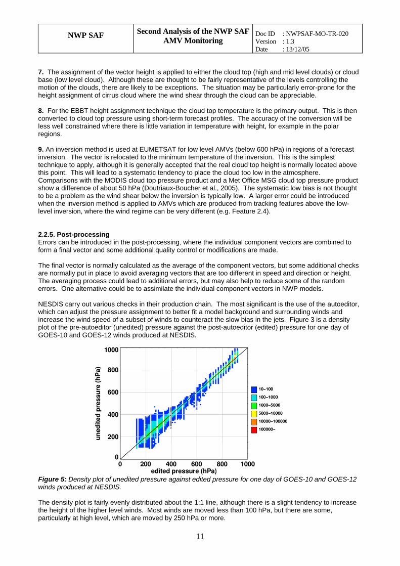
7. The assignment of the vector height is applied to either the cloud top (high and mid level clouds) or cloud base (low level cloud). Although these are thought to be fairly representative of the levels controlling the motion of the clouds, there are likely to be exceptions. The situation may be particularly error-prone for the height assignment of cirrus cloud where the wind shear through the cloud can be appreciable. 8. For the EBBT height assignment technique the cloud top temperature is the primary output. This is then converted to cloud top pressure using short-term forecast profiles. The accuracy of the conversion will be less well constrained where there is little variation in temperature with height, for example in the polar regions. 9. An inversion method is used at EUMETSAT for low level AMVs (below 600 hPa) in regions of a forecast inversion. The vector is relocated to the minimum temperature of the inversion. This is the simplest technique to apply, although it is generally accepted that the real cloud top height is normally located above this point. This will lead to a systematic tendency to place the cloud too low in the atmosphere. Comparisons with the MODIS cloud top pressure product and a Met Office MSG cloud top pressure product show a difference of about 50 hPa (Doutriaux-Boucher et al., 2005). The systematic low bias is not thought to be a problem as the wind shear below the inversion is typically low. A larger error could be introduced when the inversion method is applied to AMVs which are produced from tracking features above the low-level inversion, where the wind regime can be very different (e.g. Feature 2.4). 2.2.5. Post-processing Errors can be introduced in the post-processing, where the individual component vectors are combined to form a final vector and some additional quality control or modifications are made. The final vector is normally calculated as the average of the component vectors, but some additional checks are normally put in place to avoid averaging vectors that are too different in speed and direction or height. The averaging process could lead to additional errors, but may also help to reduce some of the random errors. One alternative could be to assimilate the individual component vectors in NWP models. NESDIS carry out various checks in their production chain. The most significant is the use of the autoeditor, which can adjust the pressure assignment to better fit a model background and surrounding winds and increase the wind speed of a subset of winds to counteract the slow bias in the jets. Figure 3 is a density plot of the pre-autoeditor (unedited) pressure against the post-autoeditor (edited) pressure for one day of GOES-10 and GOES-12 winds produced at NESDIS.
Figure 5: Density plot of unedited pressure against edited pressure for one day of GOES-10 and GOES-12 winds produced at NESDIS. The density plot is fairly evenly distributed about the 1:1 line, although there is a slight tendency to increase the height of the higher level winds. Most winds are moved less than 100 hPa, but there are some, particularly at high level, which are moved by 250 hPa or more.
NWP SAF Second Analysis of the NWP SAF AMV Monitoring
Doc ID : NWPSAF-MO-TR-020 Version : 1.3 Date : 13/12/05
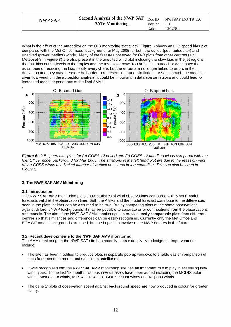
What is the effect of the autoeditor on the O-B monitoring statistics? Figure 6 shows an O-B speed bias plot compared with the Met Office model background for May 2005 for both the edited (post-autoeditor) and unedited (pre-autoeditor) winds. Many of the features observed for O-B plots from other centres (e.g. Meteosat-8 in Figure 8) are also present in the unedited wind plot including the slow bias in the jet regions, the fast bias at mid-levels in the tropics and the fast bias above 180 hPa. The autoeditor does have the advantage of reducing the bias nearly everywhere, but the errors are no longer linked to errors in the derivation and they may therefore be harder to represent in data assimilation. Also, although the model is given low weight in the autoeditor analysis, it could be important in data sparse regions and could lead to increased model dependence of the final AMVs. .
FMoF 3 3TfsaacE 3Ti •
•
•
a b
1
igure 6: O-B speed bias plots for (a) GOES-12 editeet Office model background for May 2005. The striaf the GOES winds to a limited number of vertical preigure 5.
. The NWP SAF AMV Monitoring
.1. Introduction he NWP SAF AMV monitoring plots show statistics o
orecasts valid at the observation time. Both the AMVseen in the plots; neither can be assumed to be true. gainst different NWP backgrounds, it may be possiblnd models. The aim of the NWP SAF AMV monitorinentres so that similarities and differences can be easCMWF model backgrounds are used, but the hope i
.2. Recent developments to the NWP SAF AMV mhe AMV monitoring on the NWP SAF site has recent
nclude:
The site has been modified to produce plots in sepplots from month to month and satellite to satellite
It was recognised that the NWP SAF AMV monitorwind types. In the last 18 months, various new dawinds, Meteosat-8 winds, MTSAT-1R winds, GOE
The density plots of observation speed against bacclarity.
2
d and (b) GOES-12 unedited winds compared with the tions in the left hand plot are due to the reassignment ssures in the autoeditor. This can also be seen in
f wind observations compared with 6 hour model and the model forecast contribute to the differences
But by comparing plots of the same observations e to separate error contributions from the observations g is to provide easily comparable plots from different ily recognised. Currently only the Met Office and s to involve more NWP centres in the future.
onitoring ly been extensively redesigned. Improvements
arate pop up windows to enable easier comparison of etc.
ing site has an important role to play in assessing new tasets have been added including the MODIS polar S 3.9µm winds and Kalpana winds.
kground speed are now produced in colour for greater
NWP SAF Second Analysis of the NWP SAF AMV Monitoring
Doc ID : NWPSAF-MO-TR-020 Version : 1.3 Date : 13/12/05
13
• The map statistics plots are produced individually for each satellite. Polar projections are used for the MODIS polar winds. The main advantage is greater clarity in the overlap regions between satellites.
• Map and zonal plots showing the number of winds in each geographical box are produced and a
modification made so that the statistics are only calculated for boxes containing 5 or more observations. Aside from highlighting the distribution of AMVs, they can also help to highlight discrepancies in the data displayed and have been useful for identifying missing data e.g. the lack of GOES 3.9um winds south of 20S in the Aug-Oct 2005 plots.
• Plots as a function of latitude and pressure have been added. These provide much greater information
on the vertical distribution of O-B statistics and complement the map plots. They may be particularly beneficial since height assignment is thought to be a large source of error in the AMV data.
There are several ideas for future developments, which are listed in the action list at the end of this document. 3.3. Types of plots Currently there are three types of statistical quality plot. The first is a density map of observation wind speed against background wind speed for different satellite, channel, pressure level and latitude band combinations (e.g. Figure 10). The plots show average wind speed bias, and areas of significant departure from the 1:1 line. The second type is a map of wind speed bias, mean vector difference (mvd), normalised root mean square vector difference (nrmsvd) and number plotted for different wind types (infrared, water vapour, visible) and satellites at different pressure levels (e.g. Figure 11). The third type is a zonal plot showing the same set of statistics as for the map plots but as a function of latitude and pressure (e.g. Figure 6). Together the map and zonal plots highlight geographical areas where there is significant mismatch between observations and model backgrounds. All plots of geostationary AMVs, unless stated otherwise, are produced using observations with quality indicator (QI) values greater than 80 for IR and WV winds and greater than 65 for visible winds (where the QI is the EUMETSAT-designed QI with first guess check). No QI thresholds are applied to the MODIS polar winds. Throughout this document NH is used to refer to the area north of 20N, SH is used to refer to the area south of 20S and the tropics is used to refer to the area between 20S and 20N. 4. Features observed in the O-B statistics plots 4.1. Interpreting the plots Where areas of mismatch are similar for both centres, the problems are either due to the observations not reflecting the real winds, or they are problems that are shared by the NWP models. Areas of mismatch between the two centres indicate regions where the models are treating the winds differently. This could be due to differences in the forecast models or data assimilation. There is another reason for possible differences between the Met Office and ECMWF plots and that is the choice of which winds to include in the plots. The main difference is in the WV plots where ECMWF include the clear sky and cloudy WV winds and the Met Office include only the cloudy water vapour winds. The plots showing the number of winds in each statistics box have been particularly useful at highlighting discrepancies between the two centres. Some examples are the map and zonal number plots for the GOES-9, 10 and 12 satellites, which are often different for the two centres. This is probably due to inconsistencies in the quality control applied before the statistics are calculated. To address this problem an action has been placed on the participating centres to work towards reducing these discrepancies. A note will also be attached to the NWP SAF AMV webpage detailing the recommended filtering and settings when producing the monitoring. 4.2. General observations from the plots Before identifying and discussing particular features observed in the NWP SAF AMV monitoring plots, it is worth drawing some general conclusions. Firstly, the majority of the features discussed in the following
NWP SAF Second Analysis of the NWP SAF AMV Monitoring
Doc ID : NWPSAF-MO-TR-020 Version : 1.3 Date : 13/12/05
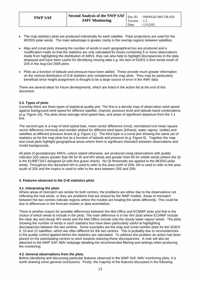
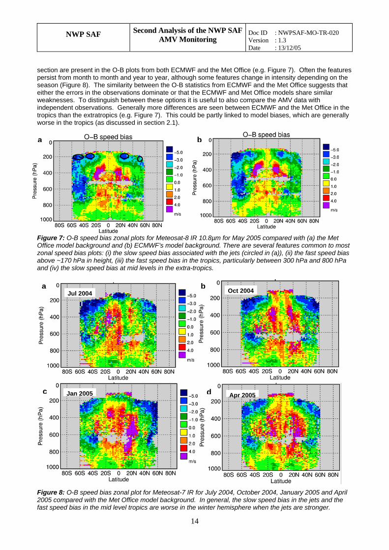
section are present in the O-B plots from both ECMWF and the Met Office (e.g. Figure 7). Often the features persist from month to month and year to year, although some features change in intensity depending on the season (Figure 8). The similarity between the O-B statistics from ECMWF and the Met Office suggests that either the errors in the observations dominate or that the ECMWF and Met Office models share similar weaknesses. To distinguish between these options it is useful to also compare the AMV data with independent observations. Generally more differences are seen between ECMWF and the Met Office in the tropics than the extratropics (e.g. Figure 7). This could be partly linked to model biases, which are generally worse in the tropics (as discussed in section 2.1).
b
aFigure 8: O-B speed bias zonal plot for Meteosat-7 IR2005 compared with the Met Office model backgrounfast speed bias in the mid level tropics are worse in th
Figure 7: O-B speed bias zonal plots for Meteosat-8 Office model background and (b) ECMWF’s model bazonal speed bias plots: (i) the slow speed bias associabove ~170 hPa in height, (iii) the fast speed bias in tand (iv) the slow speed bias at mid levels in the extra
aJul 2004
c Jan 2005
14
fd. e
IR 10.8µm for May 2005 compared with (a) the Met ckground. There are several features common to most ated with the jets (circled in (a)), (ii) the fast speed bias he tropics, particularly between 300 hPa and 800 hPa -tropics.
b
or July 2004, October 2004, January 2005 and April In general, the slow speed bias in the jets and the winter hemisphere when the jets are stronger.
Oct 2004
d Apr 2005
NWP SAF Second Analysis of the NWP SAF AMV Monitoring
Doc ID : NWPSAF-MO-TR-020 Version : 1.3 Date : 13/12/05
15
rn, this section is broken down into discussions of specific features; each ne is often evident in more than one channel and more than one type of plot. For ease of reading, these
w level (below 700 hPa), medium level (400-700 hPa) and high level (above 400 hPa)
is partly reflects the lower wind speeds in is area. There are, however, some features worth discussing further. Before doing so, it is worth
of the low level wind field. These are illustrated in Figure 9.
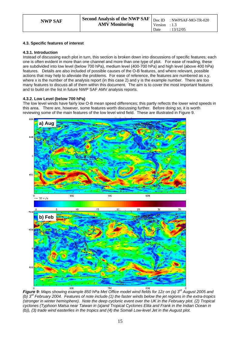
4.3. Specific features of interest 4.3.1. Introduction Instead of discussing each plot in tuoare subdivided into lofeatures. Details are also included of possible causes of the O-B features, and where relevant, possible actions that may help to alleviate the problems. For ease of reference, the features are numbered as x.y, where x is the number of the analysis report (in this case 2) and y is the example number. There are too many features to discuss all of them within this document. The aim is to cover the most important featuresand to build on the list in future NWP SAF AMV analysis reports. 4.3.2. Low Level (below 700 hPa) The low level winds have fairly low O-B mean speed differences; ththreviewing some of the main features
rdFigure 9: Maps showing example 850 hPa Met Office model wind fields for 12z on (a) 3 August 2005 and
(b) 3rd February 2004. Features of note include (1) the faster winds below the jet regions in the extra-tropics nger in winter hemisphere). Note the deep cyclonic event over the UK in the February plot. (2) Tropical (stro
b) Feb
a) Aug
cyclones (Typhoon Matsa near Taiwan in (a)and Tropical Cyclones Elita and Frank in the Indian Ocean in (b)), (3) trade wind easterlies in the tropics and (4) the Somali Low-level Jet in the August plot.
NWP SAF Second Analysis of the NWP SAF AMV Monitoring
Doc ID : NWPSAF-MO-TR-020 Version : 1.3 Date : 13/12/05
16
dicators or al dataset. One outcome of this is to introduce a fast bias at
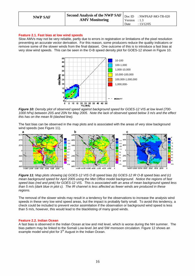
Feature 2.1. Fast bias at low wind speeds Slow AMVs may not be very reliable, partly due to errors in registration or limitations of the pixel resolution preventing an accurate vector derivation. For this reason, some producers reduce the quality inremove some of the slower winds from the finvery slow wind speeds. This can be seen in the O-B speed density plot for GOES-12 shown in Figure 10.
10-100
100-1,000
1,000-10,000
,000
10,000-100,000
100,000-1,000
1,000,000-
Figure 10: Density plot of observed speed against background speed for GOES-12 VIS at low level (700-1000 hPa) between 20S and 20N for May 2005. Note t d below 3 m/s and the effect
hed line).
a b c
he lack of observed speethis has on the mean fit (das The fast bias can be observed in the map plots and is associated with the areas of very slow background wind speeds (see Figure 11).
Figure 11: Map plots showing (a) GOES-12 VIS O-B speed bias (b) GOES-12 IR O-B speed bias and (c) mean background speed for April 2005 using the Met Office model background. Notice the regions of fast peed bias (red and pink) for GOES-12 VIS. This is associated with an area of mean background speed less
wind these very low wind speed areas, but the impact is probably fairly small. To avoid this tendency, a
heck could be included to prevent vector assimilation if the observation or background wind speed is less
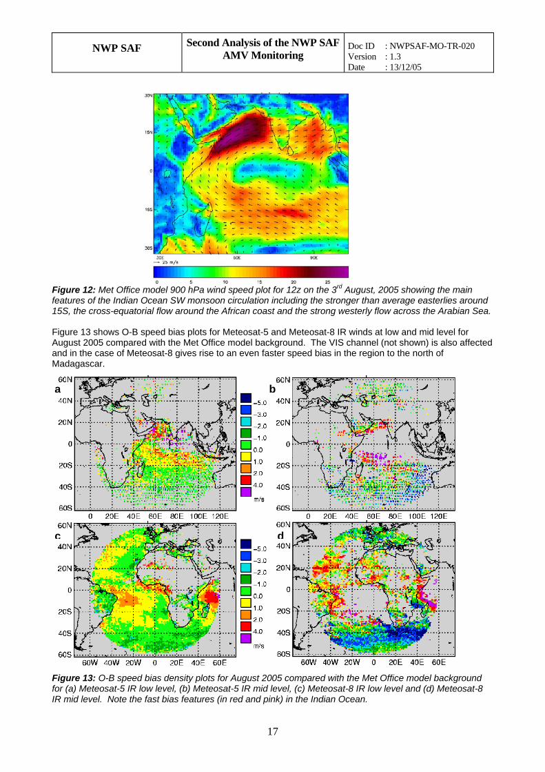
fast bias is observed in the Indian Ocean at low and mid level, which is worse during the NH summer. The ias pattern may be linked to the Somali Low-level Jet and SW monsoon circulation. Figure 12 shows an
3rd August in the Indian Ocean.
sthan 5 m/s (dark blue in plot c). The IR channel is less affected as fewer winds are produced in these regions. The removal of the slower winds may result in a tendency for the observations to increase the analysisspeeds incthan 5 m/s, however, this would lead to the blacklisting of many good winds. Feature 2.2. Indian Ocean Abexample model wind plot for
NWP SAF Second Analysis of the NWP SAF AMV Monitoring
Doc ID : NWPSAF-MO-TR-020 Version : 1.3 Date : 13/12/05
17
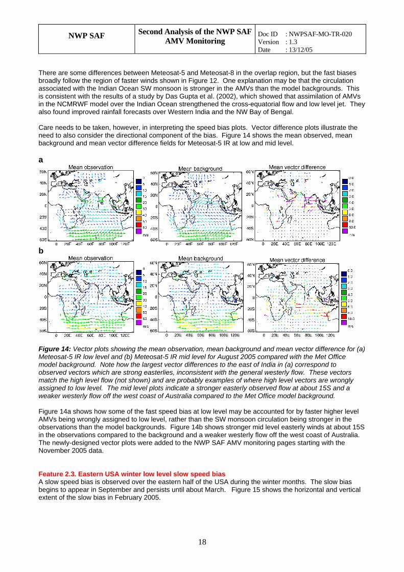
Figure 12: Met Office model 900 hPa wind speed plot for 12z on the 3rd August, 2005 showing the main features of the Indian Ocean SW monsoon circulation including the stronger than average easterlies around 15S, the cross-equatorial flow around the African coast and the strong westerly flow across the Arabian Sea. Figure 13 shows O-B speed bias plots for Meteosat-5 and Meteosat-8 IR winds at low and mid level for August 2005 compared with the Met Office model background. The VIS channel (not shown) is also affected and in the case of Meteosat-8 gives rise to an even faster speed bias in the region to the north of Madagascar.
a b
c d
Figure 13: O-B speed bias density plots for August 2005 compared with the Met Office model background for (a) Meteosat-5 IR low level, (b) Meteosat-5 IR mid level, (c) Meteosat-8 IR low level and (d) Meteosat-8 IR mid level. Note the fast bias features (in red and pink) in the Indian Ocean.
NWP SAF Second Analysis of the NWP SAF AMV Monitoring
Doc ID : NWPSAF-MO-TR-020 Version : 1.3 Date : 13/12/05
18
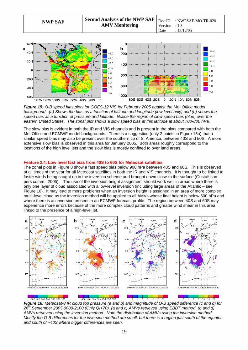
There are some differences between Meteosat-5 and Meteosat-8 in the overlap region, but the fast biases broadly follow the region of faster winds shown in Figure 12. One explanation may be that the circulation associated with the Indian Ocean SW monsoon is stronger in the AMVs than the model backgrounds. This is consistent with the results of a study by Das Gupta et al. (2002), which showed that assimilation of AMVs in the NCMRWF model over the Indian Ocean strengthened the cross-equatorial flow and low level jet. They also found improved rainfall forecasts over Western India and the NW Bay of Bengal. Care needs to be taken, however, in interpreting the speed bias plots. Vector difference plots illustrate the need to also consider the directional component of the bias. Figure 14 shows the mean observed, mean background and mean vector difference fields for Meteosat-5 IR at low and mid level. a
b
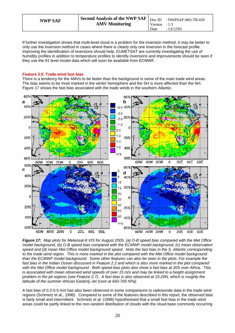
Figure 14: Vector plots showing the mean observation, mean background and mean vector difference for (a) Meteosat-5 IR low level and (b) Meteosat-5 IR mid level for August 2005 compared with the Met Office model background. Note how the largest vector differences to the east of India in (a) correspond to observed vectors which are strong easterlies, inconsistent with the general westerly flow. These vectors match the high level flow (not shown) and are probably examples of where high level vectors are wrongly assigned to low level. The mid level plots indicate a stronger easterly observed flow at about 15S and a weaker westerly flow off the west coast of Australia compared to the Met Office model background. Figure 14a shows how some of the fast speed bias at low level may be accounted for by faster higher level AMVs being wrongly assigned to low level, rather than the SW monsoon circulation being stronger in the observations than the model backgrounds. Figure 14b shows stronger mid level easterly winds at about 15S in the observations compared to the background and a weaker westerly flow off the west coast of Australia. The newly-designed vector plots were added to the NWP SAF AMV monitoring pages starting with the November 2005 data. Feature 2.3. Eastern USA winter low level slow speed bias A slow speed bias is observed over the eastern half of the USA during the winter months. The slow bias begins to appear in September and persists until about March. Figure 15 shows the horizontal and vertical extent of the slow bias in February 2005.
NWP SAF Second Analysis of the NWP SAF AMV Monitoring
Doc ID : NWPSAF-MO-TR-020 Version : 1.3 Date : 13/12/05
19
a b
Figure 15: O-B speed bias plots for GOES-12 VIS for February 2005 against the Met Office model background. (a) Shows the bias as a function of latitude and longitude (low level only) and (b) shows the speed bias as a function of pressure and latitude. Notice the region of slow speed bias (blue) over the eastern United States. The zonal plot shows a slow speed bias at this latitude at about 700-800 hPa.
The slow bias is evident in both the IR and VIS channels and is present in the plots compared with both the Met Office and ECMWF model backgrounds. There is a suggestion (only 2 points in Figure 15a) that a similar speed bias may also be present over the southern tip of S. America, between 40S and 50S. A more extensive slow bias is observed in this area for January 2005. Both areas roughly correspond to the locations of the high level jets and the slow bias is mostly confined to over land areas. Feature 2.4. Low level fast bias from 40S to 60S for Meteosat satellites The zonal plots in Figure 8 show a fast speed bias below 900 hPa between 40S and 60S. This is observed at all times of the year for all Meteosat satellites in both the IR and VIS channels. It is thought to be linked to faster winds being caught up in the inversion scheme and brought down close to the surface (Gustafsson pers comm., 2005). The use of the inversion height assignment should work well in areas where there is only one layer of cloud associated with a low-level inversion (including large areas of the Atlantic – see Figure 16). It may lead to more problems when an inversion height is assigned in an area of more complex multi-level cloud as the inversion method will be applied to all AMVs whose final height is below 600 hPa and where there is an inversion present in an ECMWF forecast profile. The region between 40S and 60S may experience more errors because of the more complex cloud patterns and greater wind shear in this area linked to the presence of a high-level jet.
a b c d
Figure 16: Meteosat-8 IR cloud top pressure (a and b) and magnitude of O-B speed difference (c and d) for 26th September 2005 0000-2100 (Only QI>70). (a and c) AMVs retrieved using EBBT method, (b and d) AMVs retrieved using the inversion method. Note the distribution of AMVs using the inversion method. Mostly the O-B differences for the inversion method are small, but there is a region just south of the equator and south of ~40S where bigger differences are seen.
NWP SAF Second Analysis of the NWP SAF AMV Monitoring
Doc ID : NWPSAF-MO-TR-020 Version : 1.3 Date : 13/12/05
20
If further investigation shows that multi-level cloud is a problem for the inversion method, it may be better to only use the inversion method in cases where there is clearly only one inversion in the forecast profile. Improving the identification of inversions should help. EUMETSAT are currently investigating the use of humidity profiles in addition to temperature profiles to identify inversions and improvements should be seen if they use the 91 level model data which will soon be available from ECMWF. Feature 2.5. Trade wind fast bias There is a tendency for the AMVs to be faster than the background in some of the main trade wind areas. The bias seems to be most marked in the winter hemisphere and the SH is more affected than the NH. Figure 17 shows the fast bias associated with the trade winds in the southern Atlantic.
a b
cd
Figure 17: Map plots for Meteosat-8 VIS for August 2005. (a) O-B speed bias compared with the Met Office model background, (b) O-B speed bias compared with the ECMWF model background, (c) mean observation speed and (d) mean Met Office model background speed. Note the fast bias in the S. Atlantic corresponding to the trade wind region. This is more marked in the plot compared with the Met Office model background than the ECMWF model background. Some other features can also be seen in the plots. For example the fast bias in the Indian Ocean discussed in Feature 2.2 and which is also more marked in the plot compared with the Met Office model background. Both speed bias plots also show a fast bias at 20S over Africa. This is associated with mean observed wind speeds of over 15 m/s and may be linked to a height assignment problem in the jet regions (see Feature 2.7). A fast bias is also observed at 15-20N, which is roughly the latitude of the summer African Easterly Jet (core at 650-700 hPa). A fast bias of 0.2-0.5 m/s has also been observed in some comparisons to radiosonde data in the trade wind regions (Schmetz et al., 1996). Compared to some of the features described in this report, the observed bias is fairly small and intermittent. Schmetz et al. (1996) hypothesised that a small fast bias in the trade wind areas could be partly linked to the non-random distribution of clouds with the cloud base commonly occurring
NWP SAF Second Analysis of the NWP SAF AMV Monitoring
Doc ID : NWPSAF-MO-TR-020 Version : 1.3 Date : 13/12/05
21
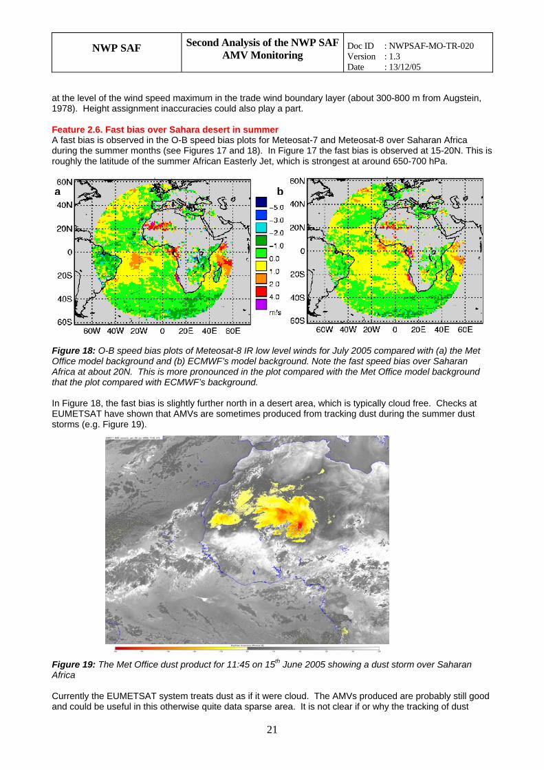
at the level of the wind speed maximum in the trade wind boundary layer (about 300-800 m from Augstein, 1978). Height assignment inaccuracies could also play a part. Feature 2.6. Fast bias over Sahara desert in summer A fast bias is observed in the O-B speed bias plots for Meteosat-7 and Meteosat-8 over Saharan Africa during the summer months (see Figures 17 and 18). In Figure 17 the fast bias is observed at 15-20N. This is roughly the latitude of the summer African Easterly Jet, which is strongest at around 650-700 hPa.
a b
Figure 18: O-B speed bias plots of Meteosat-8 IR low level winds for July 2005 compared with (a) the Met Office model background and (b) ECMWF’s model background. Note the fast speed bias over Saharan Africa at about 20N. This is more pronounced in the plot compared with the Met Office model background that the plot compared with ECMWF’s background. In Figure 18, the fast bias is slightly further north in a desert area, which is typically cloud free. Checks at EUMETSAT have shown that AMVs are sometimes produced from tracking dust during the summer dust storms (e.g. Figure 19).
Figure 19: The Met Office dust product for 11:45 on 15th June 2005 showing a dust storm over Saharan Africa Currently the EUMETSAT system treats dust as if it were cloud. The AMVs produced are probably still good and could be useful in this otherwise quite data sparse area. It is not clear if or why the tracking of dust
NWP SAF Second Analysis of the NWP SAF AMV Monitoring
Doc ID : NWPSAF-MO-TR-020 Version : 1.3 Date : 13/12/05
22
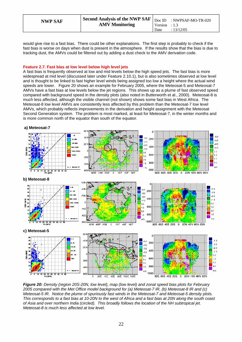
would give rise to a fast bias. There could be other explanations. The first step is probably to check if the fast bias is worse on days when dust is present in the atmosphere. If the results show that the bias is due to tracking dust, the AMVs could be filtered out by adding a dust check to the AMV derivation code. Feature 2.7. Fast bias at low level below high level jets A fast bias is frequently observed at low and mid levels below the high speed jets. The fast bias is more widespread at mid level (discussed later under Feature 2.10.1), but is also sometimes observed at low level and is thought to be linked to fast higher level winds being assigned too low a height where the actual wind speeds are lower. Figure 20 shows an example for February 2005, where the Meteosat-5 and Meteosat-7 AMVs have a fast bias at low levels below the jet regions. This shows up as a plume of fast observed speed compared with background speed in the density plots (also noted in Butterworth et al., 2000). Meteosat-8 is much less affected, although the visible channel (not shown) shows some fast bias in West Africa. The Meteosat-8 low level AMVs are consistently less affected by this problem than the Meteosat-7 low level AMVs, which probably reflects improvements in the derivation and height assignment with the Meteosat Second Generation system. The problem is most marked, at least for Meteosat-7, in the winter months and is more common north of the equator than south of the equator. a) Meteosat-7
b) Meteosat-8
c) Meteosat-5
Figure 20: Density (region 20S-20N, low level), map (low level) and zonal speed bias plots for February 2005 compared with the Met Office model background for (a) Meteosat-7 IR, (b) Meteosat-8 IR and (c) Meteosat-5 IR. Notice the plume of spuriously fast winds in the Meteosat-7 and Meteosat-5 density plots. This corresponds to a fast bias at 10-20N to the west of Africa and a fast bias at 20N along the south coast of Asia and over northern India (circled). This broadly follows the location of the NH subtropical jet. Meteosat-8 is much less affected at low level.
NWP SAF Second Analysis of the NWP SAF AMV Monitoring
Doc ID : NWPSAF-MO-TR-020 Version : 1.3 Date : 13/12/05
23
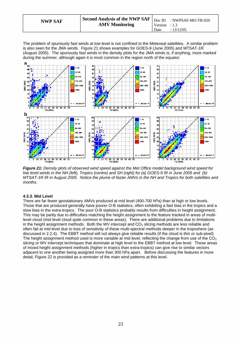
The problem of spuriously fast winds at low level is not confined to the Meteosat satellites. A similar problem is also seen for the JMA winds. Figure 21 shows examples for GOES-9 (June 2005) and MTSAT-1R (August 2005). The spuriously fast winds in the density plots for the JMA winds is, if anything, more marked during the summer, although again it is most common in the region north of the equator.
a
b
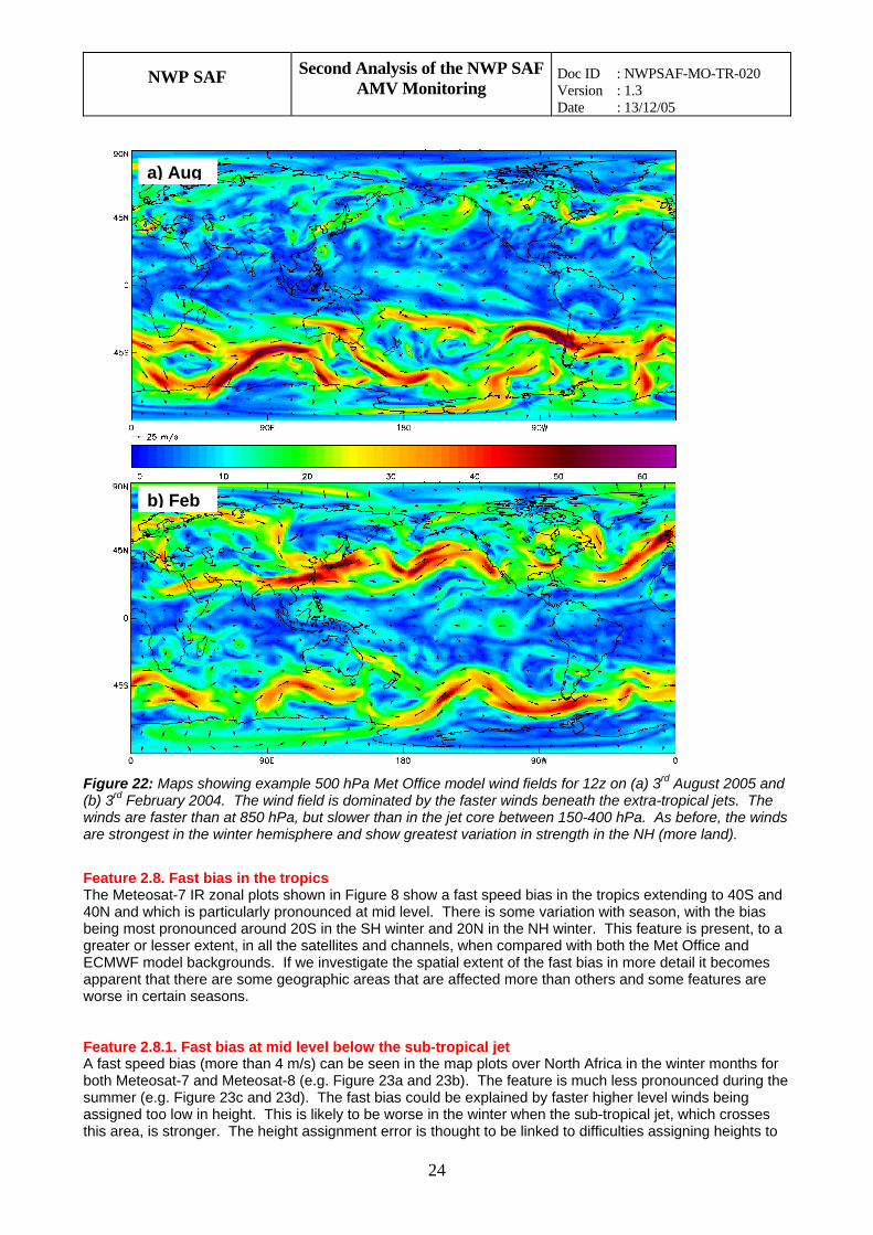
Figure 21: Density plots of observed wind speed against the Met Office model background wind speed for low level winds in the NH (left), Tropics (centre) and SH (right) for (a) GOES-9 IR in June 2005 and (b) MTSAT-1R IR in August 2005. Notice the plume of faster AMVs in the NH and Tropics for both satellites and months. 4.3.3. Mid Level There are far fewer geostationary AMVs produced at mid level (400-700 hPa) than at high or low levels. Those that are produced generally have poorer O-B statistics, often exhibiting a fast bias in the tropics and a slow bias in the extra-tropics. The poor O-B statistics probably results from difficulties in height assignment. This may be partly due to difficulties matching the height assignment to the feature tracked in areas of multi-level cloud (mid level cloud quite common in these areas). There are additional problems due to limitations in the height assignment methods. Both the WV intercept and CO2 slicing methods are less reliable and often fail at mid level due to loss of sensitivity of these multi-spectral methods deeper in the troposhere (as discussed in 2.2.4). The EBBT method will not always give reliable results (if the cloud is thin or sub-pixel). The height assignment method used is more variable at mid level, reflecting the change from use of the CO2 slicing or WV intercept techniques that dominate at high level to the EBBT method at low level. These areas of mixed height assignment methods (higher in tropics than extra-tropics) can give rise to similar vectors adjacent to one another being assigned more than 300 hPa apart. Before discussing the features in more detail, Figure 22 is provided as a reminder of the main wind patterns at this level.
NWP SAF Second Analysis of the NWP SAF AMV Monitoring
Doc ID : NWPSAF-MO-TR-020 Version : 1.3 Date : 13/12/05
24
a) Aug
b) Feb
Figure 22: Maps showing example 500 hPa Met Office model wind fields for 12z on (a) 3rd August 2005 and (b) 3rd February 2004. The wind field is dominated by the faster winds beneath the extra-tropical jets. The winds are faster than at 850 hPa, but slower than in the jet core between 150-400 hPa. As before, the winds are strongest in the winter hemisphere and show greatest variation in strength in the NH (more land).
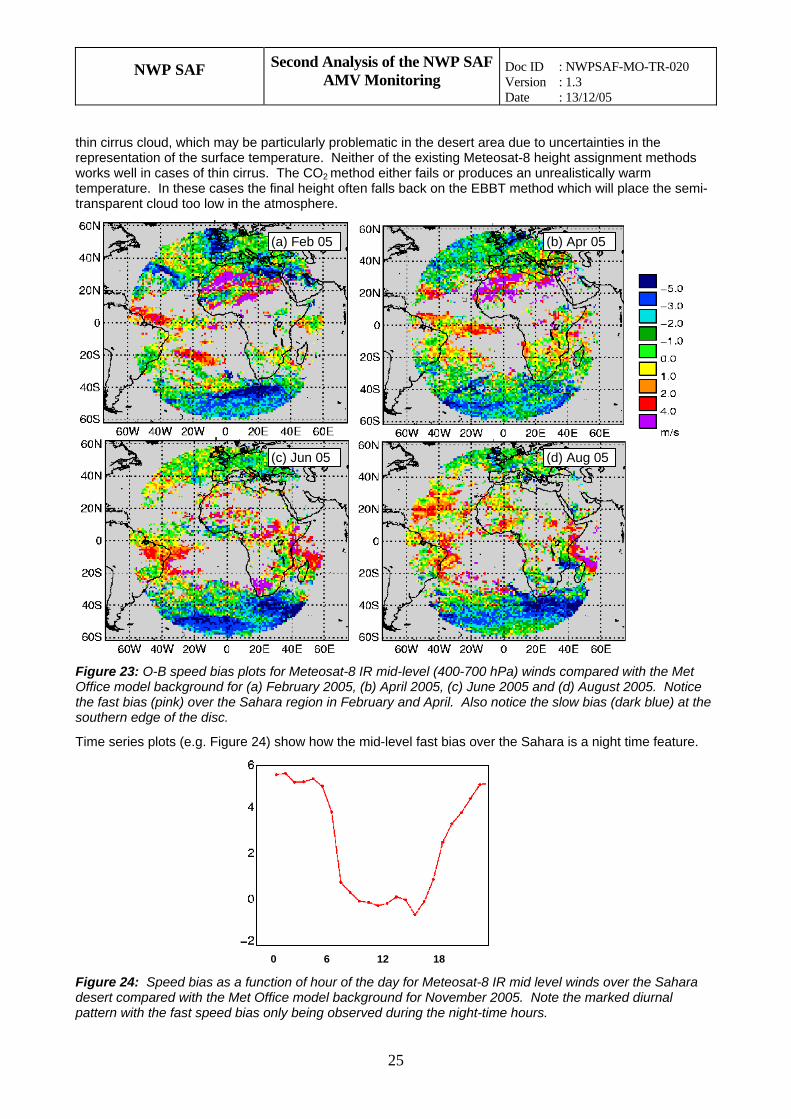
Feature 2.8. Fast bias in the tropics The Meteosat-7 IR zonal plots shown in Figure 8 show a fast speed bias in the tropics extending to 40S and 40N and which is particularly pronounced at mid level. There is some variation with season, with the bias being most pronounced around 20S in the SH winter and 20N in the NH winter. This feature is present, to a greater or lesser extent, in all the satellites and channels, when compared with both the Met Office and ECMWF model backgrounds. If we investigate the spatial extent of the fast bias in more detail it becomes apparent that there are some geographic areas that are affected more than others and some features are worse in certain seasons. Feature 2.8.1. Fast bias at mid level below the sub-tropical jet A fast speed bias (more than 4 m/s) can be seen in the map plots over North Africa in the winter months for both Meteosat-7 and Meteosat-8 (e.g. Figure 23a and 23b). The feature is much less pronounced during the summer (e.g. Figure 23c and 23d). The fast bias could be explained by faster higher level winds being assigned too low in height. This is likely to be worse in the winter when the sub-tropical jet, which crosses this area, is stronger. The height assignment error is thought to be linked to difficulties assigning heights to
NWP SAF Second Analysis of the NWP SAF AMV Monitoring
Doc ID : NWPSAF-MO-TR-020 Version : 1.3 Date : 13/12/05
25
thin cirrus cloud, which may be particularly problematic in the desert area due to uncertainties in the representation of the surface temperature. Neither of the existing Meteosat-8 height assignment methods works well in cases of thin cirrus. The CO2 method either fails or produces an unrealistically warm temperature. In these cases the final height often falls back on the EBBT method which will place the semi-transparent cloud too low in the atmosphere.
5
5 5
Figure 23: O-B speed bias plots for Meteosat-8 IR mid-level (400-700 hPa) windOffice model background for (a) February 2005, (b) April 2005, (c) June 2005 anthe fast bias (pink) over the Sahara region in February and April. Also notice thesouthern edge of the disc.
Time series plots (e.g. Figure 24) show how the mid-level fast bias over the Saha
0 6 12 18
Figure 24: Speed bias as a function of hour of the day for Meteosat-8 IR mid levdesert compared with the Met Office model background for November 2005. Nopattern with the fast speed bias only being observed during the night-time hours.
(d) Aug 0
(c) Jun 0(b) Apr 0
(a) Feb 05s compared with the Met d (d) August 2005. Notice slow bias (dark blue) at the
ra is a night time feature.
el winds over the Sahara te the marked diurnal
NWP SAF Second Analysis of the NWP SAF AMV Monitoring
Doc ID : NWPSAF-MO-TR-020 Version : 1.3 Date : 13/12/05
26
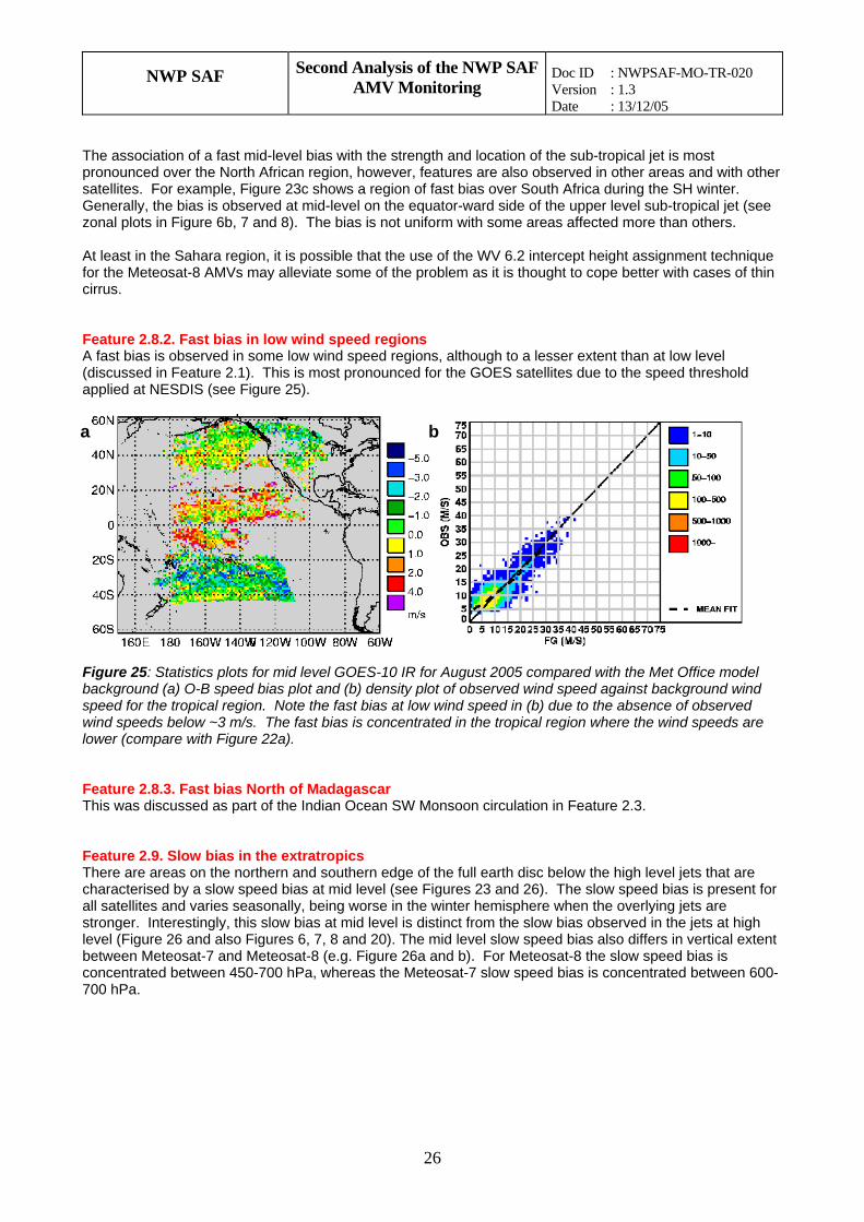
The association of a fast mid-level bias with the strength and location of the sub-tropical jet is most pronounced over the North African region, however, features are also observed in other areas and with other satellites. For example, Figure 23c shows a region of fast bias over South Africa during the SH winter. Generally, the bias is observed at mid-level on the equator-ward side of the upper level sub-tropical jet (see zonal plots in Figure 6b, 7 and 8). The bias is not uniform with some areas affected more than others. At least in the Sahara region, it is possible that the use of the WV 6.2 intercept height assignment technique for the Meteosat-8 AMVs may alleviate some of the problem as it is thought to cope better with cases of thin cirrus. Feature 2.8.2. Fast bias in low wind speed regions A fast bias is observed in some low wind speed regions, although to a lesser extent than at low level (discussed in Feature 2.1). This is most pronounced for the GOES satellites due to the speed threshold applied at NESDIS (see Figure 25).
a b
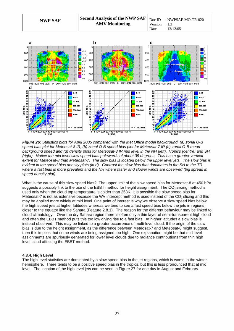
Figure 25: Statistics plots for mid level GOES-10 IR for August 2005 compared with the Met Office model background (a) O-B speed bias plot and (b) density plot of observed wind speed against background wind speed for the tropical region. Note the fast bias at low wind speed in (b) due to the absence of observed wind speeds below ~3 m/s. The fast bias is concentrated in the tropical region where the wind speeds are lower (compare with Figure 22a). Feature 2.8.3. Fast bias North of Madagascar This was discussed as part of the Indian Ocean SW Monsoon circulation in Feature 2.3. Feature 2.9. Slow bias in the extratropics There are areas on the northern and southern edge of the full earth disc below the high level jets that are characterised by a slow speed bias at mid level (see Figures 23 and 26). The slow speed bias is present for all satellites and varies seasonally, being worse in the winter hemisphere when the overlying jets are stronger. Interestingly, this slow bias at mid level is distinct from the slow bias observed in the jets at high level (Figure 26 and also Figures 6, 7, 8 and 20). The mid level slow speed bias also differs in vertical extent between Meteosat-7 and Meteosat-8 (e.g. Figure 26a and b). For Meteosat-8 the slow speed bias is concentrated between 450-700 hPa, whereas the Meteosat-7 slow speed bias is concentrated between 600-700 hPa.
NWP SAF Second Analysis of the NWP SAF AMV Monitoring
Doc ID : NWPSAF-MO-TR-020 Version : 1.3 Date : 13/12/05
27
a b c
d
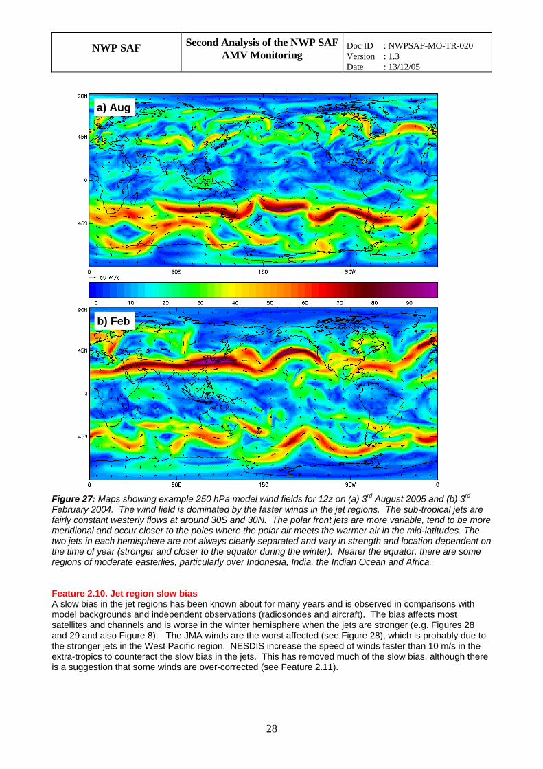
Figure 26: Statistics plots for April 2005 compared with the Met Office model background. (a) zonal O-B speed bias plot for Meteosat-8 IR, (b) zonal O-B speed bias plot for Meteosat-7 IR (c) zonal O-B mean background speed and (d) density plots for Meteosat-8 IR mid level in the NH (left), Tropics (centre) and SH (right). Notice the mid level slow speed bias polewards of about 35 degrees. This has a greater vertical extent for Meteosat-8 than Meteosat-7. The slow bias is located below the upper level jets. The slow bias is evident in the speed bias density plots (in d). Contrast the slow bias that dominates in the SH to the TR where a fast bias is more prevalent and the NH where faster and slower winds are observed (big spread in speed density plot). What is the cause of this slow speed bias? The upper limit of the slow speed bias for Meteosat-8 at 450 hPa suggests a possibly link to the use of the EBBT method for height assignment. The CO2 slicing method is used only when the cloud top temperature is colder than 253K. It is possible the slow speed bias for Meteosat-7 is not as extensive because the WV intercept method is used instead of the CO2 slicing and this may be applied more widely at mid level. One point of interest is why we observe a slow speed bias below the high speed jets at higher latitudes whereas we tend to see a fast speed bias below the jets in regions closer to the equator like the Sahara (Feature 2.8.1). The reason for the different behaviour may be linked to cloud climatology. Over the dry Sahara region there is often only a thin layer of semi-transparent high cloud and often the EBBT method puts this too low giving rise to a fast bias. At higher latitudes a slow bias is instead observed. This may be linked to a greater occurrence of multi-level cloud. If the origin of the slow bias is due to the height assignment, as the difference between Meteosat-7 and Meteosat-8 might suggest, then this implies that some winds are being assigned too high. One explanation might be that mid level assignments are spuriously generated for lower level clouds due to radiance contributions from thin high level cloud affecting the EBBT method. 4.3.4. High Level The high level statistics are dominated by a slow speed bias in the jet regions, which is worse in the winter hemisphere. There tends to be a positive speed bias in the tropics, but this is less pronounced that at mid level. The location of the high level jets can be seen in Figure 27 for one day in August and February.
NWP SAF Second Analysis of the NWP SAF AMV Monitoring
Doc ID : NWPSAF-MO-TR-020 Version : 1.3 Date : 13/12/05
28
a) Aug
b) Feb
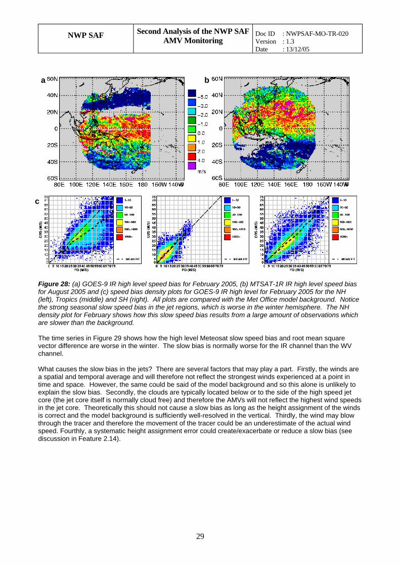
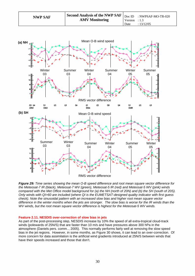
Figure 27: Maps showing example 250 hPa model wind fields for 12z on (a) 3rd August 2005 and (b) 3rd February 2004. The wind field is dominated by the faster winds in the jet regions. The sub-tropical jets are fairly constant westerly flows at around 30S and 30N. The polar front jets are more variable, tend to be more meridional and occur closer to the poles where the polar air meets the warmer air in the mid-latitudes. The two jets in each hemisphere are not always clearly separated and vary in strength and location dependent on the time of year (stronger and closer to the equator during the winter). Nearer the equator, there are some regions of moderate easterlies, particularly over Indonesia, India, the Indian Ocean and Africa. Feature 2.10. Jet region slow bias A slow bias in the jet regions has been known about for many years and is observed in comparisons with model backgrounds and independent observations (radiosondes and aircraft). The bias affects most satellites and channels and is worse in the winter hemisphere when the jets are stronger (e.g. Figures 28 and 29 and also Figure 8). The JMA winds are the worst affected (see Figure 28), which is probably due to the stronger jets in the West Pacific region. NESDIS increase the speed of winds faster than 10 m/s in the extra-tropics to counteract the slow bias in the jets. This has removed much of the slow bias, although there is a suggestion that some winds are over-corrected (see Feature 2.11).
NWP SAF Second Analysis of the NWP SAF AMV Monitoring
Doc ID : NWPSAF-MO-TR-020 Version : 1.3 Date : 13/12/05
29
a b
c
Figure 28: (a) GOES-9 IR high level speed bias for February 2005, (b) MTSAT-1R IR high level speed bias for August 2005 and (c) speed bias density plots for GOES-9 IR high level for February 2005 for the NH (left), Tropics (middle) and SH (right). All plots are compared with the Met Office model background. Notice the strong seasonal slow speed bias in the jet regions, which is worse in the winter hemisphere. The NH density plot for February shows how this slow speed bias results from a large amount of observations which are slower than the background. The time series in Figure 29 shows how the high level Meteosat slow speed bias and root mean square vector difference are worse in the winter. The slow bias is normally worse for the IR channel than the WV channel. What causes the slow bias in the jets? There are several factors that may play a part. Firstly, the winds are a spatial and temporal average and will therefore not reflect the strongest winds experienced at a point in time and space. However, the same could be said of the model background and so this alone is unlikely to explain the slow bias. Secondly, the clouds are typically located below or to the side of the high speed jet core (the jet core itself is normally cloud free) and therefore the AMVs will not reflect the highest wind speeds in the jet core. Theoretically this should not cause a slow bias as long as the height assignment of the winds is correct and the model background is sufficiently well-resolved in the vertical. Thirdly, the wind may blow through the tracer and therefore the movement of the tracer could be an underestimate of the actual wind speed. Fourthly, a systematic height assignment error could create/exacerbate or reduce a slow bias (see discussion in Feature 2.14).
NWP SAF Second Analysis of the NWP SAF AMV Monitoring
Doc ID : NWPSAF-MO-TR-020 Version : 1.3 Date : 13/12/05
30
(b) SH
Summer 05
Winter 05
Summer 05
Mean O-B wind speed
RMS vector difference
Winter 04
Summer 04
RMS vector difference
Winter 05
Mean O-B wind speed
Winter 04
Summer 04
Winter 03
Summer 03
Summer 03
Winter 03
(a) NH
Figure 29: Time series showing the mean O-B speed difference and root mean square vector difference for the Meteosat-7 IR (black), Meteosat-7 WV (green), Meteosat-5 IR (red) and Meteosat-5 WV (pink) winds compared with the Met Office model background for (a) the NH (north of 20N) and (b) the SH (south of 20S). Only winds with QI>60 are included (where QI is the EUMETSAT-designed quality indicator with first guess check). Note the sinusoidal pattern with an increased slow bias and higher root mean square vector difference in the winter months when the jets are stronger. The slow bias is worse for the IR winds than the WV winds, but the root mean square vector difference is highest for the Meteosat-5 WV winds. Feature 2.11. NESDIS over-correction of slow bias in jets As part of the post-processing step, NESDIS increase by 10% the speed of all extra-tropical cloud-track winds (polewards of 25N/S) that are faster than 10 m/s and have pressures above 300 hPa in the atmosphere (Daniels pers. comm.., 2005). This normally performs fairly well at removing the slow speed bias in the jet regions. However, in some months, as Figure 30 shows, it can lead to an over-correction. Of more concern for data assimilation is the artificial wind gradients introduced at 25N/S between winds that have their speeds increased and those that don’t.
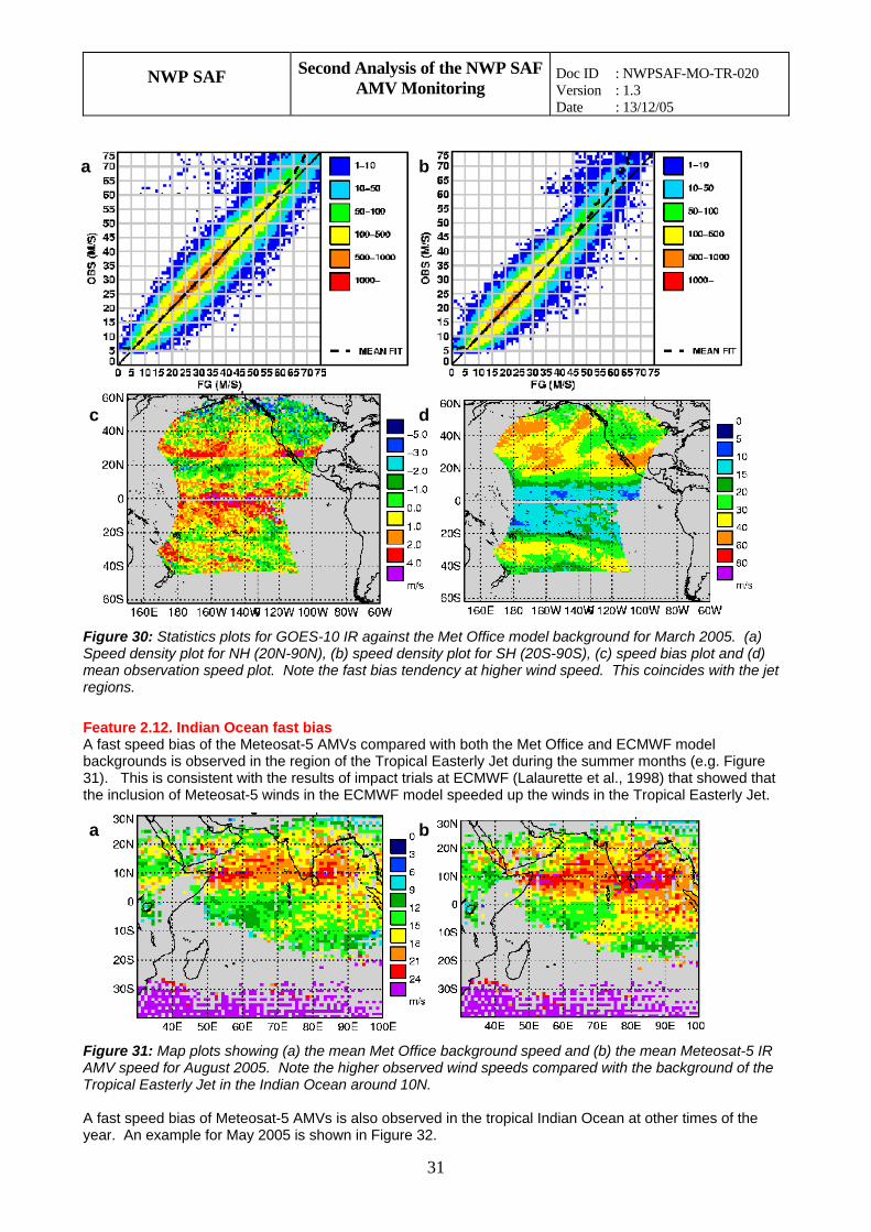
NWP SAF Second Analysis of the NWP SAF AMV Monitoring
Doc ID : NWPSAF-MO-TR-020 Version : 1.3 Date : 13/12/05
31
a b
c d
Figure 30: Statistics plots for GOES-10 IR against the Met Office model background for March 2005. (a) Speed density plot for NH (20N-90N), (b) speed density plot for SH (20S-90S), (c) speed bias plot and (d) mean observation speed plot. Note the fast bias tendency at higher wind speed. This coincides with the jet regions.
Feature 2.12. Indian Ocean fast bias A fast speed bias of the Meteosat-5 AMVs compared with both the Met Office and ECMWF model backgrounds is observed in the region of the Tropical Easterly Jet during the summer months (e.g. Figure 31). This is consistent with the results of impact trials at ECMWF (Lalaurette et al., 1998) that showed that the inclusion of Meteosat-5 winds in the ECMWF model speeded up the winds in the Tropical Easterly Jet.
a b
Figure 31: Map plots showing (a) the mean Met Office background speed and (b) the mean Meteosat-5 IR AMV speed for August 2005. Note the higher observed wind speeds compared with the background of the Tropical Easterly Jet in the Indian Ocean around 10N. A fast speed bias of Meteosat-5 AMVs is also observed in the tropical Indian Ocean at other times of the year. An example for May 2005 is shown in Figure 32.
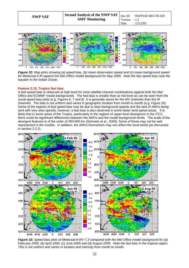
NWP SAF Second Analysis of the NWP SAF AMV Monitoring
Doc ID : NWPSAF-MO-TR-020 Version : 1.3 Date : 13/12/05
32
a b c
Figure 32: Map plots showing (a) speed bias, (b) mean observation speed and (c) mean background speed for Meteosat-5 IR against the Met Office model background for May 2005. Note the fast speed bias near the equator in the Indian Ocean.
Feature 2.13. Tropics fast bias A fast speed bias is observed at high level for most satellite-channel combinations against both the Met Office and ECMWF model backgrounds. The fast bias is smaller than at mid level as can be seen from the zonal speed bias plots (e.g. Figures 6, 7 and 8) It is generally worse for the WV channels than the IR channels. The bias is not uniform and varies in geographic location from month to month (e.g. Figure 33). Some of the regions of fast speed bias may be due to slow background speeds and the lack of AMVs being sent with very slow speeds, however, a fast bias is also observed in some faster wind speed areas. It is likely that in some areas of the Tropics, particularly in the regions of upper level divergence in the ITCZ, there could be significant differences between the AMVs and the model background winds. The scale of the divergent features is of the order of 300-500 km (Schmetz et al., 2004). Some of these may not be well represented in the models. In addition, the AMVs themselves may not reflect the local winds (as discussed in section 2.2.2).
a Feb 05 b Apr 05
c Jun 05 d Aug 05
Figure 33: Speed bias plots of Meteosat-8 WV 7.3 compared with the Met Office model background for (a) February 2005, (b) April 2005, (c) June 2005 and (d) August 2005. Note the fast bias in the tropical region. This is not uniform and varies in location and intensity from month to month.
NWP SAF Second Analysis of the NWP SAF AMV Monitoring
Doc ID : NWPSAF-MO-TR-020 Version : 1.3 Date : 13/12/05
33
Feature 2.14. Very high level (above 180 hPa) fast bias Many of the satellite-channel combinations display a fast bias at very high levels (above 180 hPa in height). This is most prevalent for the GOES unedited winds (e.g. Figure 6), but is also visible in many of the Meteosat zonal plots (e.g. Figures 7 and 8), although there is some variation from month to month in its latitudinal extent. It is not yet clear what causes this bias. If it is a model error then it is something that is shared by the ECMWF and Met Office models. Feature 2.15. Differences between channels There are some notable differences between the IR and WV statistics for some satellites. The biggest differences are seen for the AMVs produced by JMA (GOES-9 and MTSAT-1R). The zonal plots in Figure 34 show how the slow speed bias is worse for GOES-9 IR than the GOES-9 cloudy WV winds.
ba
Figure 34: O-B speed bias plots for (a) GOES-9 IR and (b) GOES-9 cloudy WV for May 2005 compared with the Met Office model background. Figure 35 shows how the NH O-B speed bias and root mean square vector difference varies with season. Again, notice the much greater slow speed bias and root mean square vector difference for the IR channel compared with the WV channel.
IR
WV
Summer 05
Winter 05
Summer 03
Winter 03
Summer 04
Winter 04
Mean O-B wind speed
RMS vector difference
Figure 35: Time series plot showing monthly O-B speed bias and root mean square vector difference for the JMA SATOB IR (green) and JMA SATOB WV (pink) winds compared with the Met Office model background for the NH. Note the marked increase in slow speed bias and root mean square vector difference in the winter months. This is much more marked for the IR than the WV and is worse following the change to automatic quality control in 2003.
NWP SAF Second Analysis of the NWP SAF AMV Monitoring
Doc ID : NWPSAF-MO-TR-020 Version : 1.3 Date : 13/12/05
34
One possible source of the different behaviour of the two channels could be the height assignment. To test this hypothesis, we plotted the GOES-9 WV heights against the GOES-9 IR heights for collocated pairs of winds (see Figure 36). The scatter plot shows that the cloudy WV winds are consistently located lower in the atmosphere by, on average, ~50 hPa. Because clouds are not evenly distributed, tending to be located below the high speed jet core (e.g. England & Ulbrecht, 1980), a systematic height assignment error could contribute to or counteract a slow speed bias. Notice also how the fast speed bias in the tropics is worse for the cloudy WV winds than the IR. In this case a systematic lowering of the height assignment would exacerbate an existing fast speed bias.
Figure 36: Scatter plot comparing the height assignment of collocated GOES-9 IR and GOES-9 cloudy WV winds. The cloudy WV winds are consistently located lower in the atmosphere, by on average, about 50 hPa. There are also some differences between the Meteosat-8 IR and WV channels. Figure 37 shows scatter plots of the u component, v component and height assignment of collocated Meteosat-8 WV winds and Meteosat-8 IR 10.8 winds. Some variation might be expected between the channels in areas of multi-level cloud as they are sensitive to different layers of the atmosphere. Despite this, the u and v components of the IR and WV 6.2 channels agree well, which may suggest that the channels are normally tracking the same feature. The height assignment, however, shows more variability. The IR and WV heights compare well at high levels (above ~230 hPa for WV 6.2 and above ~350 hPa for WV 7.3). Below this, the heights start to diverge with the WV winds located systematically higher in the atmosphere.
ba c
Figure 37: Scatter plots of collocated (a) Meteosat-8 WV 6.2 against Meteosat-8 IR u-component, (b) Meteosat-8 WV 6.2 against Meteosat-8 IR v-component and (c) Meteosat-8 WV 6.2 (green) and WV 7.3 (black) against Meteosat-8 IR height assignment for 10:30 on the 13th April 2005. Note the good agreement of the u and v components, but the tendency for the WV winds to be assigned higher in height particularly at lower levels.
There are two principal height assignment techniques at high and mid level for the Meteosat-8 winds. These are the EBBT and CO2 slicing techniques. The CO2 slicing technique will normally be applied when the cloud top temperature is less than 253K. The exception is the use of the EBBT method when the EBBT
NWP SAF Second Analysis of the NWP SAF AMV Monitoring
Doc ID : NWPSAF-MO-TR-020 Version : 1.3 Date : 13/12/05
35
cloud top temperature is colder than the CO2 slicing cloud top temperature. This only occurs 5-10% of the time for the IR 10.8 and WV 7.3 channels, but about half the time for the WV 6.2 channel (Doutriaux-Boucher et al., 2005). A higher percentage is not surprising for the WV 6.2 channel since it peaks higher in the atmosphere and therefore the WV 6.2 EBBT is less likely to put semi-transparent cloud too low compared with the WV 7.3 EBBT or IR 10.8 EBBT. However,~50% does seem high and may suggest a problem with the WV 6.2 EBBT height assignment method. The increasing divergence between the IR and WV heights at lower levels suggests that the WV EBBT cold bias becomes worse for vectors lower in the atmosphere. This could be partly affected by a bug which meant EUMETSAT were not allowing for atmospheric absorption above cloud top in the radiative transfer code for the Meteosat-8 winds before 1st December 2005, but other factors such as calibration error may also play a role. Not allowing for WV absorption above cloud top would be more marked for vectors lower down the weighting function and could explain the observed increase in height difference at lower levels. The WV 7.3 heights shows better agreement with the IR 10.8, but there is still a divergence at lower levels in the atmosphere, probably reflecting the different location of the weighting function (see Figure 38).
Figure 38: Standard mid-latitude summer nadir normalised weighting functions for different MSG channels. Of main interest are the WV 6.2 (in red), WV 7.3 (in green) and IR 10.8 (in magenta). Investigations at EUMETSAT into the differences have highlighted some areas where the IR and WV vectors are consistent, but the height assignments are different. The example in Figure 39 shows better forecast consistency for the IR AMVs, although it is not yet clear whether this is normally the case.
ba
Figure 39: Meteosat-8 AMVs producing from tracking features in (a) IR 10.8 and (b) WV 7.3 channels, overlain on their respective imagery. The numbers in white, yellow or blue are the heights in hPa, the numbers in green are the forecast consistency scores against an ECMWF forecast. Note the circled AMVs, where the IR and WV height assignments are very different (~620 hPa for IR and ~470 hPa for WV 7.3). The forecast consistency is better for the IR winds than the WV winds and might suggest the IR height assignment is closer to the truth. Pictures courtesy of Jörgen Gustafsson (EUMETSAT).
NWP SAF Second Analysis of the NWP SAF AMV Monitoring
Doc ID : NWPSAF-MO-TR-020 Version : 1.3 Date : 13/12/05
36
Given the tendency for WV winds to be located higher in the atmosphere it might be expected that they would exhibit a larger slow bias in the extra-tropics and a smaller fast bias in the tropics (i.e. the opposite of the pattern observed for the JMA winds). The biases for Meteosat-8, however, cannot be as easily explained. Contrary to the expected pattern, the fast bias in the tropics is worse for the WV AMVs (see Figure 40). a b c
Figure 40: O-B speed bias zonal plots for (a) Meteosat-8 IR 10.8, (b) Meteosat-8 WV 7.3 and (c) Meteosat-8 WV 6.2 for April 2005 compared with the Met Office model background. 4.3.5. Polar winds MODIS polar winds are produced at both CIMSS and NESDIS. It was agreed at the 7th International Winds Workshop that all new developments to the MODIS AMV product would be tested first at CIMSS and then migrated to the operational system at NESDIS. To help in the assessment of the changes, monitoring of both the CIMSS and NESDIS MODIS winds are included on the NWP SAF site. Before CIMSS implement any changes, they are trying to ensure the two products are very similar. Most of the NWP SAF plots for the MODIS winds from the two centres are alike, but some differences are highlighted below. It should be noted that the NWP SAF AMV monitoring only includes data that arrives in time for the model cut-offs. Feature 2.16. Number of MODIS IR winds It had been noted from the NWP SAF number plots that there were proportionately more IR MODIS winds in the NESDIS dataset than in the CIMSS dataset. To investigate further, the percentage of total winds from each channel from both centres was calculated. The results for May 2005 are shown in Table 1 and confirm that a greater proportion of the NESDIS MODIS dataset is IR AMVs compared with CIMSS (38% versus 16%). This was brought to the attention of CIMSS and NESDIS, who implemented a change on the 2nd August. The results for September 2005 are also shown in Table 1 and indicate that the number of IR winds is now more similar, but there are still some differences.
May 2005 Sep 2005
NESDIS CIMSS NESDIS CIMSS
IR 38% 16% 36% 30% Cloudy WV 23% 35% 25% 37%
Clear sky WV 39% 49% 39% 34% Table 1: Percentage of AMVs from each channel for the NESDIS and CIMSS MODIS datasets for May 2005 and September 2005. Note the greater percentage of IR winds from NESDIS in May. This is less marked in September, but some differences are still apparent. Feature 2.17. CIMSS MODIS mid level fast winds Another difference that is occasionally seen is in the speed bias density plots for mid level winds. Sometimes the CIMSS data density plots show a plume of spuriously fast winds (e.g. Figure 41). These are not observed in the equivalent NESDIS plots. A plume has been observed in all channels (IR, cloudy WV,
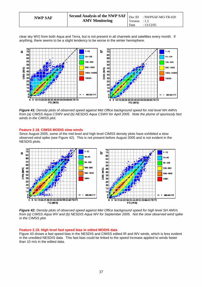
NWP SAF Second Analysis of the NWP SAF AMV Monitoring
Doc ID : NWPSAF-MO-TR-020 Version : 1.3 Date : 13/12/05
37
clear sky WV) from both Aqua and Terra, but is not present in all channels and satellites every month. If anything, there seems to be a slight tendency to be worse in the winter hemisphere.
ba
Figure 41: Density plots of observed speed against Met Office background speed for mid level NH AMVs from (a) CIMSS Aqua CSWV and (b) NESDIS Aqua CSWV for April 2005. Note the plume of spuriously fast winds in the CIMSS plot. Feature 2.18. CIMSS MODIS slow winds Since August 2005, some of the mid level and high level CIMSS density plots have exhibited a slow observed wind spike (see Figure 42). This is not present before August 2005 and is not evident in the NESDIS plots.
a b
Figure 42: Density plots of observed speed against Met Office background speed for high level SH AMVs from (a) CIMSS Aqua WV and (b) NESDIS Aqua WV for September 2005. Not the slow observed wind spike in the CIMSS plot. Feature 2.19. High level fast speed bias in edited MODIS data Figure 43 shows a fast speed bias in the NESDIS and CIMSS edited IR and WV winds, which is less evident in the unedited NESDIS data. This fast bias could be linked to the speed increase applied to winds faster than 10 m/s in the edited data.
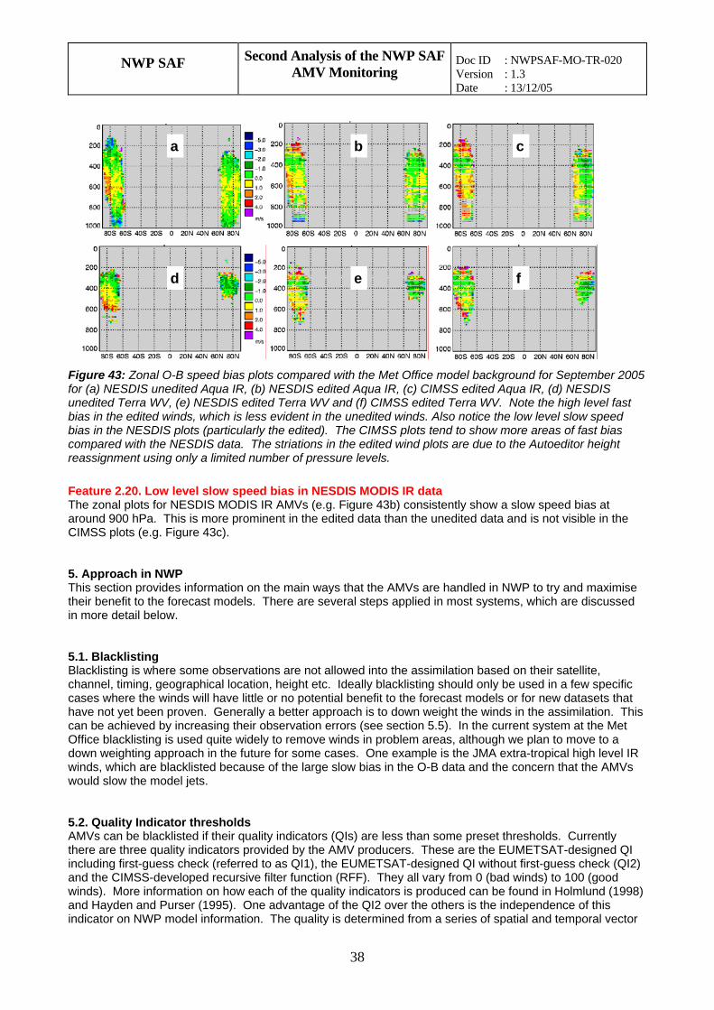
NWP SAF Second Analysis of the NWP SAF AMV Monitoring
Doc ID : NWPSAF-MO-TR-020 Version : 1.3 Date : 13/12/05
38
a b c
d e f
Figure 43: Zonal O-B speed bias plots compared with the Met Office model background for September 2005 for (a) NESDIS unedited Aqua IR, (b) NESDIS edited Aqua IR, (c) CIMSS edited Aqua IR, (d) NESDIS unedited Terra WV, (e) NESDIS edited Terra WV and (f) CIMSS edited Terra WV. Note the high level fast bias in the edited winds, which is less evident in the unedited winds. Also notice the low level slow speed bias in the NESDIS plots (particularly the edited). The CIMSS plots tend to show more areas of fast bias compared with the NESDIS data. The striations in the edited wind plots are due to the Autoeditor height reassignment using only a limited number of pressure levels.
Feature 2.20. Low level slow speed bias in NESDIS MODIS IR data The zonal plots for NESDIS MODIS IR AMVs (e.g. Figure 43b) consistently show a slow speed bias at around 900 hPa. This is more prominent in the edited data than the unedited data and is not visible in the CIMSS plots (e.g. Figure 43c). 5. Approach in NWP This section provides information on the main ways that the AMVs are handled in NWP to try and maximise their benefit to the forecast models. There are several steps applied in most systems, which are discussed in more detail below. 5.1. Blacklisting Blacklisting is where some observations are not allowed into the assimilation based on their satellite, channel, timing, geographical location, height etc. Ideally blacklisting should only be used in a few specific cases where the winds will have little or no potential benefit to the forecast models or for new datasets that have not yet been proven. Generally a better approach is to down weight the winds in the assimilation. This can be achieved by increasing their observation errors (see section 5.5). In the current system at the Met Office blacklisting is used quite widely to remove winds in problem areas, although we plan to move to a down weighting approach in the future for some cases. One example is the JMA extra-tropical high level IR winds, which are blacklisted because of the large slow bias in the O-B data and the concern that the AMVs would slow the model jets. 5.2. Quality Indicator thresholds AMVs can be blacklisted if their quality indicators (QIs) are less than some preset thresholds. Currently there are three quality indicators provided by the AMV producers. These are the EUMETSAT-designed QI including first-guess check (referred to as QI1), the EUMETSAT-designed QI without first-guess check (QI2) and the CIMSS-developed recursive filter function (RFF). They all vary from 0 (bad winds) to 100 (good winds). More information on how each of the quality indicators is produced can be found in Holmlund (1998) and Hayden and Purser (1995). One advantage of the QI2 over the others is the independence of this indicator on NWP model information. The quality is determined from a series of spatial and temporal vector
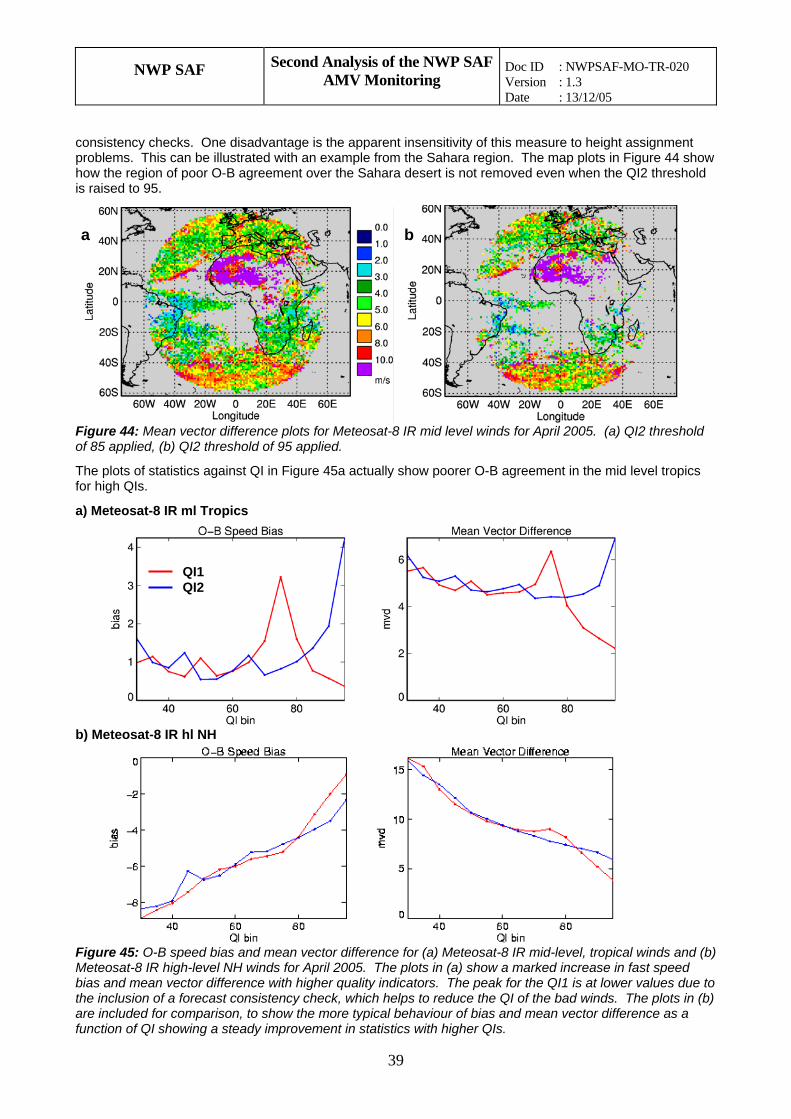
NWP SAF Second Analysis of the NWP SAF AMV Monitoring
Doc ID : NWPSAF-MO-TR-020 Version : 1.3 Date : 13/12/05
39
consistency checks. One disadvantage is the apparent insensitivity of this measure to height assignment problems. This can be illustrated with an example from the Sahara region. The map plots in Figure 44 show how the region of poor O-B agreement over the Sahara desert is not removed even when the QI2 threshold is raised to 95.
ba
Figure 44: Mean vector difference plots for Meteosat-8 IR mid level winds for April 2005. (a) QI2 threshold of 85 applied, (b) QI2 threshold of 95 applied.
The plots of statistics against QI in Figure 45a actually show poorer O-B agreement in the mid level tropics for high QIs.
a) Meteosat-8 IR ml Tropics
QI1 QI2
b) Meteosat-8 IR hl NH
Figure 45: O-B speed bias and mean vector difference for (a) Meteosat-8 IR mid-level, tropical winds and (b) Meteosat-8 IR high-level NH winds for April 2005. The plots in (a) show a marked increase in fast speed bias and mean vector difference with higher quality indicators. The peak for the QI1 is at lower values due to the inclusion of a forecast consistency check, which helps to reduce the QI of the bad winds. The plots in (b) are included for comparison, to show the more typical behaviour of bias and mean vector difference as a function of QI showing a steady improvement in statistics with higher QIs.
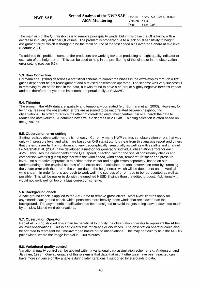
NWP SAF Second Analysis of the NWP SAF AMV Monitoring
Doc ID : NWPSAF-MO-TR-020 Version : 1.3 Date : 13/12/05
40
ck of QI sensitivity to height el
roblem, some of the producers are working towards producing a height quality indicator or stimate of the height error. This can be used to help in the pre-filtering of the winds or in the observation
.3. Bias Correction ormann et al. (2002) describes a statistical scheme to correct the biases in the extra-tropics through a first
ht reassignment and a revised observation operator. The scheme was very successful
.4. Thinning he errors in the AMV data are spatially and temporally correlated (e.g. Bormann et al., 2003). However, for
ns the observation errors are assumed to be uncorrelated between neighbouring
based on
.5. Observation error setting etting realistic observation errors is not easy. Currently many NWP centres set observation errors that vary
h are based on O-B statistics. It is clear from this analysis report and others
g rtical
.6. Background check background check is applied to the AMV data to remove gross errors. Most NWP centres apply an
heck, which penalises more heavily those winds that are slower than the much
.7. Observation Operator ao et al. (2002) showed how it can be beneficial to modify the observation operator to represent the AMVs
particularly true for clear sky WV winds. The observation operator could also
.8. Variational quality control ariational quality control can be applied within a variational data assimilation scheme (e.g. Andersson and
of this system is that data that might otherwise have been rejected can have more influence on the analysis during later iterations if supported by surrounding data.
The main aim of the QI thresholds is to remove poor quality winds, but in this case the QI is failing with a decrease in quality at higher QI values. The problem is probably due to a laassignment error, which is thought to be the main source of the fast speed bias over the Sahara at mid lev(Feature 2.8.1). To address this peerror setting (section 5.5). 5Bguess dependent heigin removing much of the bias in the data, but was found to have a neutral or slightly negative forecast impactand has therefore not yet been implemented operationally at ECMWF. 5Ttechnical reasoobservations. In order to reduce the effect of correlated error, most centres thin or superob the data to reduce the data volume. A common box size is 2 degrees or 200 km. Thinning selection is oftenthe QI values. 5Sonly with pressure level and whicthat the errors are far from uniform and vary geographically, seasonally as well as with satellite and channel. Le Marshall et al. (2004) have developed a method for generating individual observation errors for each AMV. This uses the components of the QI1 (speed, direction, vector and spatial consistency checks and comparison with first guess) together with the wind speed, wind shear, temperature shear and pressure level. An alternative approach is to estimate the vector and height errors separately, based on our understanding of the physical sources of the errors and to calculate the total observation error by summinthe vector error with the error in the vector due to the height error, which will be dependent on the vewind shear. In order for this approach to work well, the sources of error need to be represented as well as possible. This will be easier to do with the unedited NESDIS winds than the edited product. Additionally itwould not work well on top of a bias correction scheme. 5Aasymmetric background cbackground. The asymmetric modification has been designed to avoid the jets being slowed down tooby the slow-biased wind observations. 5Ras layer observations. This isbe adapted to represent the time-averaged nature of the observations. This may particularly help the MODISpolar winds, where the image interval is ~100 minutes. 5VJärvinen, 1998). One advantage
NWP SAF Second Analysis of the NWP SAF AMV Monitoring
Doc ID : NWPSAF-MO-TR-020 Version : 1.3 Date : 13/12/05
41
pted that we re not yet seeing full benefit from this data type, probably due to the complicated nature of the errors, which re often biased, non-Gaussian and correlated both with each other and with the forecast-background used
ction.
Met Office and ECMWF model backgrounds. Many of the features persist from onth to month and year to year, although some features change in intensity depending on the season.
omplicated. In some cases the height assignment is based on a different cloud level to that which s
e to inter
s,
to remove or down weight nly the data we think is more suspect. To do this, we need to have access to quality indicators that reflect
rvations. The information obtained from these investigations could be
sed to identify parts of the AMV derivation that can be improved, and to develop vector and height quality
P
f new datasets such as the MTSAT-1R and GOES .9µm winds. It can also be used to compare datasets such as the NESDIS MODIS winds with the CIMSS
the ld allow NWP centres
better exploit the information in NWP models.
ttp://www.metoffice.com/research/interproj/nwpsaf/satwind_report/action_list.html
6. Conclusions AMVs are an important source of wind information for use in NWP models. It is generally acceaain the wind produ The examples included in Section 4 of this paper demonstrate how the NWP SAF AMV monitoring can be used to improve our understanding of the errors in the AMV data. Generally the monthly plots are similar when compared with the mMany of the examples of speed biases can be explained by errors in the height assignment. Unsurprisingly the speed biases are often worse in the jet regions, where the wind speed changes rapidly with height. In these regions, an error in the height assignment could give rise to a large error in the vector wind speed. From the discussion of the sources of AMV error in section 2, it is expected that some situations may be more likely to give rise to larger AMV errors. One example is regions of multi-level cloud. The larger errorsin these regions can be understood as both the tracking and the height assignment are likely to be more cdominated in the tracking (e.g. Figure 2). Two examples of features that may be due to difficulties in regionof multi-level cloud are a fast bias at low level on the southern edge of the Meteosat area (Feature 2.4) and the slow speed bias at mid-level below the extra-tropical jets (Feature 2.9). Another region that gives risa larger speed bias is the desert. This is most apparent at mid level over the Sahara during the NH w(Feature 2.8.1). The fast speed bias is thought to be linked to difficulties assigning heights to thin cirrus cloud, possibly partly linked to poor representation of the surface temperatures. Of concern for NWP is that some of the most significant bias features are not reflected in the current qualityindicators as illustrated in Figures 44 and 45. Often in these situations we end up blacklisting whole regionin some cases removing perfectly good winds. A more sensible approach is to try othe errors in the data effectively. To continue improving our knowledge of the errors, it would be useful to undertake a thorough analysis of the limitations of the AMV derivation in combination with continuing statistical comparisons of the AMV data withmodel backgrounds and other obseuindicators that effectively reflect the errors in the data. The quality indicators can be used to improve the representation of the AMV errors in NWP. This should, in combination with other developments discussed in Section 5, lead to greater impact of AMV data in NWP. Although this paper has concentrated on what we can learn about the errors in the AMV data from the NWSAF monitoring, it should be emphasised that there are other uses of this facility. The NWP SAF AMV monitoring aims to provide early statistical comparisons o3MODIS winds or the Meteosat-8 winds with the Meteosat-7 winds. The AMV Monitoring Report also provides links to summaries of AMV work and links to other AMV monitoring sites. The site is intended to stimulate thought and discussion. It is hoped that the results and analyses together with further investigations by the wind producers and NWP centres will lead to improved knowledge oferrors, which should help to target areas of development in wind derivation, and shouto 7. Revised Action List The NWP SAF AMV action list can be viewed at: h . This will be updated
very 6 months or when a significant change is made and will be fully revised on the completion of each evised action list is included below and provides suggestions of possible
developments to the site and ideas for investigating some of the observation-background inconsistencies
eanalysis of results. The r

NWP SAF Second Analysis of the NWP SAF AMV Monitoring
Doc ID : NWPSAF-MO-TR-020 Version : 1.3 Date : 13/12/05
42
he action list represent ideas for future work as opposed to on
further. It is important to realise that the items in ta formal task list. The items will be addressed, when time allows, in priority order. We welcome feedbackany of the items in the action list, including any additional suggestions for follow-up work. 7.1. Discrepancies between contributors Ref Action Details Centre(s) 1.1 Ensure consistent WV
treatment. ECMWF WV plots show statistics for cloudy and clear sky WV winds. In future should
clude cloudy.
ECMWF
only in1.3 Ensure consistent treatment
re stats are Plots showing number of winds plotted for 2
show some unexpected differences.
g. Contributors to
MetO, ECMWF of winds befocalculated.
centres Suspect possible inconsistent use of pre-filtering. Guidance to be provided on recommended filterinfollow this guidance
1.4 of ensity plots e
e major problem. If
N/A Ensure consistent displayspeed bias d
ECMWF use a variable colour scale and box size. This was hard to replicate so thMet Office plots do not have identical format. As long as users are aware of thdifferences it is not athere is concern we could exchange data and produce all the plots at the Met Office. Currently no action recommended.
7.2. Improvements to site design Ref Action Centre(s) Details 2.5 Provide guidance for future
contributors Includes information on the recommended pre-filtering.
MetO
2.6 Include a log of old completed actions.
MetO
7.3. De f plots
Ref Details Centre(s)
velopment o
Action 3.6 Develop mean vector
difference plots Both centres produce a version of these for other purposes, but they could be usefully displayed on this site.
MetO, ECMWF
3.10 Develop time series plots Lower priority unless strong demand MetO, ECMWF 3.11 Develop plots comparing
tion riority unless strong demand WF
AMVs to other observatypes.
Lower p MetO, ECM
3.12 Inclusion of plots from other uidance. Other to
MetO and other centres.
Met Office to provide gcontributors to carry out work requiredgenerate the intermediate statistics
contributors
3.15 hannels
To allow fairer comparison. MetO, ECMWF Change to use QI>80 for visible c
7.4. Analysis of results
a o ac is of the results diUpdate ll be produced every 2 years to coincide with the International Winds Workshops or
hen significant new material is available.
This p per forms the conclusion ts to this report wi
tion 4.1 to produce an analys splayed so far.
w

NWP SAF Second Analysis of the NWP SAF AMV Monitoring
Doc ID : NWPSAF-MO-TR-020 Version : 1.3 Date : 13/12/05
43
Details Centre(s) Ref Action 4.2 Provide routine updates Update analysis every two years. Update
action list every 6 months or when signifi
MetO
cant changes take place. 7.5. Fo Ref Action Centre(s)
llow up investigations
Details 5.1 Investigate model-model
differences. Investigate particular areas where the plots differ between the Met Office and ECMWF.
MetO, ECMWF
5.3 Investigate NESDIS unedited winds
Now being monitored at the Met Office MetO, ECMWF
5.4 Investigate mid level biases ular, investigate whether the extra-
s discussed in Feature 2.9).
WF In partictropical slow bias is mostly in regions of multi-level cloud and the fast bias in regions of mostly thin high level cloud (hypothesi
MetO, ECM
5.5 Fast bias at low wind speed Investigate if there is evidence that this is speeding up NWP analyses in low wind speed areas. If so consider action.
MetO, ECMWF
5.6 Diurnal variation s.
MetO, ECMWF Investigate whether there is a diurnal effecton some of the O-B feature
5.7 General height assignment investigations s
l of
Continue investigations into differences between channels and satellites in regionof overlap and comparisons with levebest-fit in model wind profiles.
MetO, ECMWF
8. Furt dations This section does not form part of the as a summary of some of the ideas voiced over the last few yea erivation and assimilation. Those onsidered higher priority are shown in bold.
Centre(s)
her recommen
NWP SAF AMV action list, but is providedrs on how to improve the AMV d
c 8.1. Recommendations for producers Ref Action Details 6.1 Documentation of
methods AMV producers to provide a document comparing the main steps in the AMV
ivation and height assignment so differences can be easily identified. This
help in the interpretation of the
All producers
der
should O-B plots, particularly where the problems differ from producer to producer.
6.2 Comparison of methods All producers Production of AMVs from each other’s imagery to directly compare different derivation schemes.
6.3 Use of simulated imagery as a test of the AMV
d realistic simulated imagery.
ry lds as
system.
ECMWF and all producers
derivation
ECMWF can now produce fairly highresolution anAMVs derived from the simulated imagecan be compared to the NWP wind fiea test of the derivation
6.4 Develop vector and height QIs/errors
To consider each step in the derivaand assess the possible sources of error. What information can be used to develop vector and height QIs/errors?
tion All producers
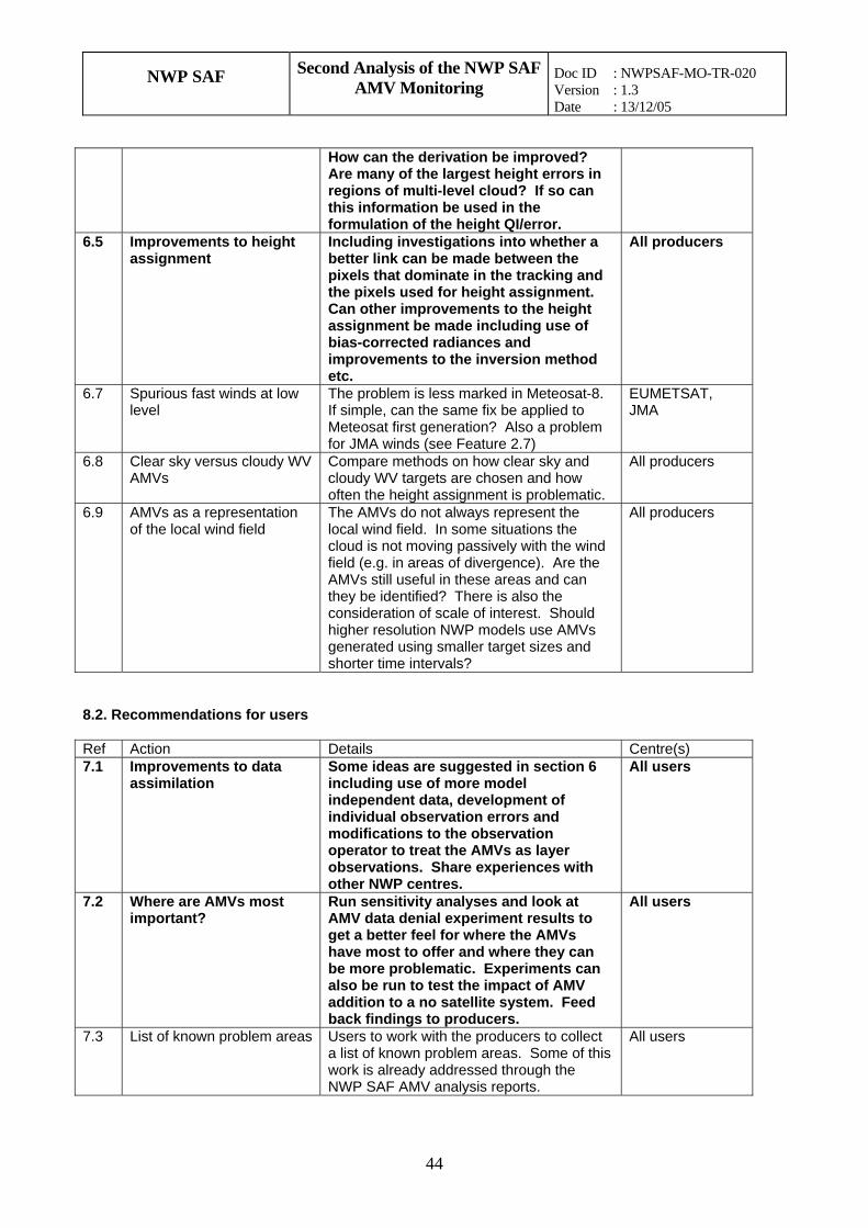
NWP SAF Second Analysis of the NWP SAF AMV Monitoring
Doc ID : NWPSAF-MO-TR-020 Version : 1.3 Date : 13/12/05
44
oved?
n
How can the derivation be imprAre many of the largest height errors in regions of multi-level cloud? If so cathis information be used in the formulation of the height QI/error.
6.5 Improvements to height assignment
ment.
All producers Including investigations into whether a better link can be made between the pixels that dominate in the tracking andthe pixels used for height assignCan other improvements to the height assignment be made including use of bias-corrected radiances and improvements to the inversion method etc.
6.7 Spurious fast winds at low level
.
a problem
EUMETSAT, JMA
The problem is less marked in Meteosat-8If simple, can the same fix be applied to Meteosat first generation? Also for JMA winds (see Feature 2.7)
6.8 Clear sky versus cloudy WV hods on how clear sky and All producers AMVs
Compare metcloudy WV targets are chosen and how often the height assignment is problematic.
6.9 AMVs as a representation of the local wind field s the
d e
d
All producers The AMVs do not always represent the local wind field. In some situationcloud is not moving passively with the winfield (e.g. in areas of divergence). Are thAMVs still useful in these areas and can they be identified? There is also the consideration of scale of interest. Shoulhigher resolution NWP models use AMVs generated using smaller target sizes and shorter time intervals?
8.2. Recommendations for users Ref Action Centre(s) Details 7.1 Improvements to data
assimilation Some ideas are suggested in section 6 including use of more model independent data, development of individual observation errors and
ations to the observation
ces with
All users
modificoperator to treat the AMVs as layer observations. Share experienother NWP centres.
7.2 Where are AMVs most important?
at ts to
Experiments can
All users Run sensitivity analyses and look AMV data denial experiment resulget a better feel for where the AMVs have most to offer and where they can be more problematic.also be run to test the impact of AMV addition to a no satellite system. Feed back findings to producers.
7.3 List of known problem areas
All users Users to work with the producers to collecta list of known problem areas. Some of thiswork is already addressed through the NWP SAF AMV analysis reports.
NWP SAF Second Analysis of the NWP SAF AMV Monitoring
Doc ID : NWPSAF-MO-TR-020 Version : 1.3 Date : 13/12/05
45
9. Acknowledgements The authors would like to thank Roge o Schmetz, Régis Borde, Jörgen Gustafsson and Niels Borman cument. They would also like to
ank Antonio Garcia-Mendez for providing the ECMWF monthly statistics and Sarah Watkin and Una ’Keefe for managing the NWP SAF website. Many of the ideas discussed in the report have been greatly
TSAT, CIMSS and ECMWF and in particular the input of Jörgen Gustafsson, Arthur
ugstein, E., 1978. The atmospheric boundary layer over the tropical oceans. In: Meteorology over the ropical Oceans. Edited by D. B. Shaw, Royal Meteorological Society, p73-103.
ing esoscale flows. Submitted to Journal of Applied Meteorology.
echniques with Meteosat-8. roceedings of the 7 International Winds Workshop, Helsinki.
nd correcting speed biases in atmospheric otion vectors within the ECMWF assimilation system. Proceedings of the 6th International Winds
ormann, N, S. Saarinen, G. Kelly and J-N Thépaut, 2003. The spatial structure of observation errors in
rette, B.J. Conway and A. Garcia-Mendez, 2000. The NWP SAF integrated satellite ind monitoring report. Proceedings of the 5th International Winds Workshop, Lorne, Australia.
V. Singh, 002. Impact of high density atmospheric motion vectors in NCMRWF global data assimilation forecast
aniels, J., C. Velden, W. Bresky and A. Irving, 2004. Status of the NOAA/NESDIS operational satellite wind e
outriaux-Boucher, M., M. Forsythe, R. Saunders and P. Francis, 2005. MSG wind height assignment
rologie, Transpress, VEB Verlag fuer Verkehrwesen, Berlin, p403.
going development of satellite-derived winds at ESDIS/CIMSS. Proceedings of the Developments in the use of satellite dat in NWP, ECMWF.
95. Recursive filter objective analysis of meteorological fields: applications NESDIS operational processing. Journal of Applied Meteorology, 34, 3-15.
vectors to erive quality indicators. Weather Forecasting, 13, 1093-1104.
f the wind field. Proceedings f the 8 Meteosat Scientific Uses Meeting, Sweden.
g SATOB products at ECMWF: availability , uality control and impact. Proceedings of the 4 International Winds Workshop, Switzerland.
r Saunders, Bryan Conway, John Eyre, Jn for suggestions to improve this do
thOhelped by visits to EUMEde Smet, Greg Dew and Jaime Daniels. 10. References Andersson, E. and H. Järvinen, 1998. Variational quality control. ECMWF Technical Memorandum 250. AT Bedka, K.M. and Mecikalski, 2005. Application of satellite-derived atmospheric motion vectors for estimatm Borde, R. and A. Arriaga, 2004. Atmospheric motion vectors height assignment t
thP Bormann, N., G. Kelly and J-N. Thépaut, 2002. Characterising amWorkshop, Wisconsin. Batmospheric motion vectors from geostationary satellite data. Monthly Weather Review, ?, ?. Butterworth, P., F. Lalauw Das Gupta, M., A.K. Mitra, S.C. Kar, V.S. Prasad, G.R., Iyengar, D. Rajan, R.K. Paliwal and S.2system. Proceedings of the 6th International Winds Workshop, Wisconsin. Dproduct system: recent improvements, new products, product quality and future plans. Proceedings of th7th International Winds Workshop, Helsinki. Dproblems. Met Office NWP Technical Report in draft. England, J. and H. Ulbricht, 1980. Flugmeteop Hayden, C.M., S.J. Nieman and T.J. Schmit. 1993. OnN Hayden, C.M. and R.J. Purser, 19to Holmlund, K., 1998. The utilization of statistical properties of satellite-derived atmospheric motiond Holmlund, K. and J. Schmetz, 1990. Cloud displacement as a representative o
tho Lalaurette, F., A. Garcia-Mendez and M. Rohn, 1998. Monitorin
thq
NWP SAF Second Analysis of the NWP SAF AMV Monitoring
Doc ID : NWPSAF-MO-TR-020 Version : 1.3 Date : 13/12/05
46
Dunn, 2004. Error characterisation of atmospheric otion vectors. Australian Meteorological Magazine, 53, 123-131
ude ssignment using VAS. Journal of Climate and Applied Meteorology, 22, 377-384.
opical performance. 1- Diagnosing errors the New Unified Model (cycle G27). Met Office NWP Technical Report 401.
J. Daniels, 1997. Fully utomated cloud drift winds in NESDIS operations. Bulletin of the American Meteorological Society, 78,
ieman, S.J., J. Schmetz and W.P. Menzel, 1993. A comparison of several techniques to assign heights to
S. Velden and S.A. Braun, 2002. The vertical error characteristics of GOES-derived winds: escription and experiments with Numerical Weather Prediction. Journal of Applied Meteorology, 41, 253-
antek, D., C.S. Velden and J.R. Key, 2004. Polar winds from MODIS: project status. Proceedings of the 7th
zin, R. and Y. Zaitseva, 2004. Modis polar winds assimilation impact study with CMC operational NWP ystem. Proceedings of the 7th International Winds Workshop, Helsinki.
omparison of cloud motion vector height assignment techniques sing the GOES-12 imager. Proceedings of the 6th International Winds Workshop, Wisconsin, USA.
. Comparison of cloud motion ector height assignment techniques using the GOES-12 imager. Proceedings of the 7th International Winds
chmetz, J., R. Borde, M. König and H-J Lutz, 2004. Upper tropospheric divergence fields in a tropical
chmetz, J., K. Holmlund, J. Hoffman, B. Stauss, B. Mason, V. Gaertner, A. Koch and L. Van der Berg, ,
chmetz, J., K. Holmlund and A. Ottenbacher, 1996. Low-level winds from high resolution visible imagery.
nd M. Nuret, 1989. Cloud motion wind estimates in Europe. ECMWF/EUMETSAT workshop, he use of satellite data in operational NWP.
e Meteosat IR and WV channels for loud studies and wind extraction. Proceedings of the 10 Meteosat Scientific Users Conference, Portugal.
nsparent cirrus cloud temperature from infrared radiances: pplications to Meteosat, Journal of Applied Meteorology, 21, 384-393.
pact studies at ECMWF. Proceedings of the 7 International Winds Workshop, Helsinki.
Le Marshall, J., A. Rea, L. Leslie, R. Seecamp and M. m Menzel, W.P., W.L. Smith and T.R. Stewart, 1983. Improved cloud motion wind vector and altita Milton, S., I. Culverwell, G. Greed and M. Willett, 2003. Improving trin Nieman, S.J., W.P. Menzel, C.M. Hayden, D. Gray, S.T. Wanzong, C.S. Velden anda1121-1133. Ncloud tracers. Journal of Applied Meteorology, 32, 1559-1568. Rao, P.A., C.d270. SInternational Winds Workshop, Helsinki. Sarras Schreiner, A.J. and W.P. Menzel, 2002. Cu Schreiner, A.J., W.P. Menzel, A. Heidinger, J. Davies and W. Feltz, 2004vWorkshop, Helsinki. Sconvective system observed with Meteosat-8. Proceedings of the 7th International Winds Workshop, Helsinki. S1993. Operational cloud-motion winds from Meteosat infrared images. Journal of Applied Meteorology, 321206-1225. SProceedings of the 3rd International Winds Workshop, Switzerland. Schmetz, J. aT Schmetz, J., L. van de Berg and V. Gaertner, 1994. Calibration of th
thc Szejwach, G., 1982. Determination of semi-traa von Bremen, L., J-N, Thépaut and G. Kelly, 2004. Assimilation of polar winds and recent satellite winds
thim