SATELLITE ALTIMETRY AND KEY OBSERVATIONS: WHAT WE’VE LEARNED,

AND WHAT’S POSSIBLE WITH NEW TECHNOLOGIES

Robert B. Scott (1)

, Mark Bourassa(2)

, Dudley Chelton(3)

, Paolo Cipollini(4)

, Raffaele Ferrari(5)

, Lee-Lueng Fu(6)

,

Boris Galperin(7)

, Sarah Gille(8)

, Huei-Ping Huang(9)

, Patrice Klein(10)

, Nikolai Maximenko(11)

, Rosemary

Morrow(12)

, Bo Qiu(13)

, Ernesto Rodriguez(6)

, Detlef Stammer(14)

, Remi Tailleux(15)

, Carl Wunsch(5)

(1) The University of Texas at Austin, 10100 Burnet Rd. Austin, TX 78758 USA, and the National Oceanography Centre,

Southampton, Waterfront Campus, European Way, Southampton SO14 3ZH, UK, Email: r.b.scott@soton.ac.uk (2)

COAPS (Center for Ocean-Atmospheric Prediction Studies), Florida State University, 236 R. M. Johnson Bldg.

32306-2840 Tallahassee USA, Email: bourassa@coaps.fsu.edu (3)

COAS (College of Oceanic and Atmospheric Sciences), Oregon State University, 104 Oceanography Admin. Bldg.,

Corvallis, OR 97331-5503 USA, Email: chelton@coas.oregonstate.edu (4)

National Oceanography Centre, Southampton, Waterfront Campus, European Way, Southampton SO14 3ZH,

United Kingdom, Email: cipo@noc.soton.ac.uk (5)

Dept. of Earth, Atmospheric, and Planetary Sciences, Massachusetts Institute of Technology, 77 Massachusetts Ave.

Cambridge, MA 02139, USA, Email: rferrari@mit.edu; cwunsch@mit.edu (6)

Jet Propulsion Laboratory, M/S 300-323, 4800 Oak Grove Drive, Pasadena, CA 91109 USA,

Email: llf@pacific.jpl.nasa.gov; ernesto.rodriguez@jpl.nasa.gov (7)

University of South Florida, College of Marine Science, 140 7th Avenue South, St. Petersburg, FL 33701, USA,

Email: bgalperin@marine.usf.edu (8)

Scripps Institution of Oceanography, University of California San Diego, 9500 Gilman Drive, San Diego, La Jolla,

CA 92093-0225, USA, Email: sgille@ucsd.edu (9)

Department of Mechanical and Aerospace Engineering, Arizona State University, PO Box 2260, Tempe,

AZ 85280-2260 USA, Email: hp.huang@asu.edu (10)

LPO, IFREMER (Laboratoire de Physique des Océans/French Institute for exploitation of the Sea/Institut Français

de Recherche pour l'Exploitation de la Mer), BP 70, 29280 Plouzané, France, Email: patrice.Klein@ifremer.fr (11)

IPRC/SOEST (International Pacific Research Center/School of Ocean and Earth Science and Technology),

University of Hawaii, 1680 East West Road, POST Bldg. #401, Honolulu, HI 96822, USA,

Email: maximenk@hawaii.edu (12)

LEGOS/OMP (Laboratoire d’Études en Géophysique et Océanographie Spatiales/L'Observatoire Midi Pyrénées),

14 Avenue Edouard Belin, 31400 Toulouse, France, Email: rosemary.morrow@cnes.fr (13)

SOEST (School of Ocean and Earth Science and Technology,) University of Hawaii at Manoa, 1000 Pope Road,

Honolulu, HI 96822, USA, Email: bo@soest.hawaii.edu (14)

Universität Hamburg, Zentrum für Marine und Atmosphärische Wissenschaften, Institut für Meereskunde,

Bundesstr. 53; 1. Stock; Raum 140, D-20146 Hamburg, Germany, Email: stammer@ifm.uni-hamburg.de (15)

Department of Meteorology, University of Reading, Earley Gate, PO Box 243, Reading, RG6 6BB, UK,

Email: r.g.j.tailleux@reading.ac.uk

INTRODUCTION

The advent of high accuracy satellite altimetry in the

1990‘s brought the first global view of ocean

dynamics, which together with a global network of

supporting observations brought a revolution in

understanding of how the ocean works [1]. At present a

constellation of flying satellite missions routinely

provides sea level anomaly, sea winds, sea surface

temperature (SST), ocean colour, etc. with mesoscale

resolution (50km to 100km, 20 to 150 days) on a near

global scale. Concurrently, in situ monitoring is carried

out by surface drifters, Argo floats, moorings, sea

gliders as well as ship-borne CTD (Conductivity-

Temperature-Depth) and XBT (Expendable

Bathythermograph) (to measure profiles of temperature

and salinity), and ADCP (Acoustic Doppler Current

Profiler) (to measure current velocity profiles).

This global observational system allowed observational

oceanography to develop into an essentially

quantitative science. This became possible because 1)

the accuracy and volume of observations exceeded

critical values, 2) numerous studies demonstrated good

agreement between independent datasets, and critically

3) the data resolution crossed the threshold of revealing

much of the mesoscale in two-dimensions, when

previously it was only revealed in one-dimension along

satellite ground tracks [2] with wide gaps in between.

Fortuitously computing power kept pace allowing

basin scale numerical ocean models to cross the

threshold of revealing the mesoscale around the turn of

the century [3]. The mesoscale is characterized by the

most energetic motions and strong nonlinear

interactions, issuing in a more complex range of

phenomena. Below in Sect. 1 we present some

highlights of this development. In Sect. 2, we describe

future prospects, and Sect. 3 provides a reminder of the

importance of maintaining continuity of high-quality

observations. We conclude in Sect. 4 with discussion

of integrating optimizing the observing system.

The benefits to society from development of

quantitative dynamical oceanography, as with most

scientific disciplines, while indirect, are no less real.

Ocean dynamics forms an important foundation for

climate dynamics and biological oceanography,

developments of which have direct impacts on

agriculture and fishing. A critical development in the

last decade has been global ocean forecasting, which

was non-existent before the Global Ocean Data

Assimilation Experiment (GODAE). Assimilation of

satellite altimeter data, SST data, and in situ Argo data

are all critical elements, without which GODAE could

not be possible.

This white paper comes at a critical juncture in ocean

observing. While the utility of the observing network is

firmly grounded in the success of the past, and

technological advances promise the possibility of

substantial gains, we still lack the commitment for

sustained funding of even the existing observing

network. We wish to express herein our sincere

concern for the future of ocean observing, and in

particular the satellite altimeter and supporting

observations (especially scatterometer and drifter data).

1. PROGRESS IN OCEANOGRAPHY FROM

SATELLITE ALTIMETRY AND SUPPORTING

OBSERVATIONS

1.1 Global View of Linear Rossby Waves

i) Theoretical understanding of complexity of linear

Rossby waves

Linear standard normal-mode theory (LST hereafter)

was, prior to satellite altimetry, the main framework for

oceanic Rossby waves. Some important features of the

standard Rossby wave modes are: 1) that they are all

stable and energetically decoupled; 2) that they have a

period that increases with latitude up to several years at

high-latitude, 3) that they are nearly nondispersive at

low wavenumbers (i.e. equal group and phase speeds at

long wavelengths), 4) that they are strongly dispersive

at high wavenumbers, with the zonal phase speed

approaching zero as the wavenumbers increase.

Nearly all these characteristics appear to be

inconsistent to various degrees with those of westward

propagating signals (WPS) observed in satellite

altimeter data collected over the past 17 years. Given

the gross simplifications of the LST, it is perhaps not

surprising that LST does not fit the observations well.

But interestingly [4] (CS96 hereafter) found observed

phase speeds, as measured by the Radon Transform

(RT hereafter), to be systematically faster by a factor of

up to two to three than the longwave phase speed

predicted by the LST for the first baroclinic mode at

mid- and high-latitudes. Furthermore, [5] suggest that

actual westward propagation is nearly nondispersive

throughout the whole wavenumber range. These results

prompted much theoretical work over the past decade.

The main results are that the background zonal mean

flow [6] and rough topography [7] are each, on their

own, able to bring theoretical phase speeds closer to

CS96's RT phase speed estimates in the long wave

limit, although room for improvement exists. The best

agreement is achieved by combining the effects of a

background mean flow and variable bottom topography

[8], [9], [10] and [11] but theoretical issues remain

open. With regard to dispersion, the background mean

flow can potentially make Rossby waves nondispersive

at high-wavenumbers [12]. Reference [13] suggests

that combined barotropic-baroclinic mode Rossby

waves might explain the non-dispersive variability

observed in the North Pacific. Reference [14] find

secondary peaks in the RT, which they interpreted as

evidence of higher-baroclinic modes, though another

possibility would be nonlinear eddies, see Sect. 1.2

below.

ii) Climatic importance of linear Rossby waves

The ocean impacts human society through marine

resources and Earth‘s climate. The tropical Pacific

phenomenon of El Nino-Southern Oscillation (ENSO)

provides a well-known example whose coupled

atmosphere-ocean nature and global impacts have been

appreciated since the 1980s. Below we describe

another important example, the Pacific Decadal

Oscillation (PDO), one of the largest climate signals in

the North Hemisphere [15]. Here too observationally

driven ocean science was essential for developing our

understanding of the coupled climate system.

It is now well established that the large-scale, wind-

induced sea surface height (SSH) variability is

controlled by baroclinic Rossby wave dynamics (e.g.

[16], [17], [18], [19], [20] and [21]). Specifically, the

large-scale SSH changes can be hindcast by integrating

the anomalous wind-stress curl forcing along the

Rossby wave characteristics along a latitude line from

the eastern boundary.

Figure 1a shows the altimeter-derived SSH anomaly

signals averaged in the latitudinal band of 32-34°N in

the North Pacific Ocean as a function of time and

longitude. Notice that the decadal SSH changes in the

eastern North Pacific can be qualitatively explained by

the wind stress curl variability associated with

the PDO, with centre of action around 160°W.

Specifically, when the PDO index is positive (see

Fig. 1c), the Aleutian Low intensifies and shifts

southward, and this works to generate negative SSH

anomalies near 160°W in the eastern North Pacific

through surface wind stress driven Ekman divergence.

The opposite is true when the PDO index is negative:

wind-induced Ekman convergence in this case results

in regional, positive SSH anomalies near 160°W. SSH

anomalies generated in the eastern North Pacific tend

to propagate westward at the speed of baroclinic

Rossby waves of ~ 3.8 cm/s, taking many years to

cross the basin to reach the Kuroshio Extension east of

Japan.

Figure 1b shows the time-longitude plot of the SSH

anomaly field in the same 32-34°N band modeled by

the linear Rossby wave model with the use of the

monthly wind stress curl data from the National

Centers for Environmental Prediction-National Center

for Atmospheric Research (NCEP-NCAR) reanalysis

[22]. As expected, the Rossby wave model captures

well all of the large-scale SSH anomaly signals that

change sign on decadal timescales. The linear

correlation coefficient between the observed and

modeled SSH anomaly fields is r = 0.45 and this

coefficient increases to 0.53 when only the interannual

SSH signals are retained in Fig. 1a. This quantitative

comparison confirms the notion that the decadal

Kuroshio Extension modulations detected by the

satellite altimeter data over the past 15 years are

initiated by the incoming SSH anomaly signals

generated by the PDO-related wind forcing in the

eastern North Pacific.

Figure 1: (a) SSH anomalies along the zonal band of 32-34°N from the satellite altimeter data. (b) Same as panel a) but

from the wind-forced baroclinic Rossby wave model. (c) PDO index from http://jisao.washington.edu/pdo/PDO.latest.

Figure from [20].

1.2 The Nonlinear Threshold

While the revolution in the 1990s came from the first

global monitoring of the ocean, the revolution of the

present decade has come from crossing the more subtle

but equally important barrier of increased

spatial/temporal resolution. The larger scale motions in

the ocean are mostly linear phenomena, albeit with

nonlinearity arising from coupling with atmospheric

phenomena, e.g. ENSO and the PDO. In contrast the

mesoscale motions (dozens to a few hundreds of

kilometers) are governed by nonlinear dynamics,

characterized by strong self-interaction of oceanic

eddies. Nonlinearity generically brings more

complexity [23]. Theoretical dynamical models since

the 1970s predict a rich phenomenology ([24], [25],

[26], [27], [28], [29] and [30] and many others) yet

with only local and scant observational support. Only

in the last few years has it been possible to observe the

nonlinear phenomena and quantify their interactions.

Traditional altimeters in exact-repeat missions measure

sea-surface height (SSH) along intersecting ground

tracks. The regions between tracks form diamond

patterns within which SSH is never sampled. Multiple

altimeters operating simultaneously significantly

improve the sampling. The degree to which this

improves the resolution of SSH fields depends on the

energy level of unresolved mesoscale variability, how

well coordinated the orbit parameters are (repeat

period, orbit inclination and measurement accuracy),

the amount of spatial and temporal smoothing applied

to the observations, and the subjectively chosen

tolerance for residual errors [31]. The residual errors

for a given amount of smoothing can vary

geographically and temporally in complicated ways,

especially for small amounts of smoothing.

For a single satellite like Jason-2, constructed SSH

fields have a resolution of about 6° in wavelength. The

resolution is approximately doubled to about 3° for

SSH fields constructed from observations from two

altimeters (Jason-2 and ENVISAT (Environmental

Satellite)), or even tripled to about 2° resolution with

well-coordinated missions like Jason-2 and Jason-1

[31]. For Gaussian eddies, these wavelength

resolutions of 6°, 3° and 2° correspond to e-folding

eddy scales of 80 km, 60 km and 40 km, respectively.

The above results apply to the smoothing procedure

applied by AVISO (Archiving, Validation and

Interpretation of Satellites Oceanographic data) [32] to

construct SSH fields from Jason-2 and ENVISAT and

their predecessor combinations of one altimeter in a

10-day repeat orbit (TOPEX (Ocean TOPography

Experiment)/Poseidon followed by Jason-1) and

another altimeter in a 35-day repeat orbit (ERS-1

followed by ERS-2 (European Remote Sensing

satellite)). The variability is attenuated for wavelengths

shorter than about 3°, see also [33].

i) Propagating features

The doubling of the spatial resolution of sea-surface

height (SSH) fields constructed by AVISO [32] from

the merged measurements by two simultaneously

operating altimeters (one in a 10-day repeat orbit and

the other in a 35-day repeat orbit) has dramatically

altered the earlier interpretation of westward

propagating variability based on TOPEX/Poseidon data

only. It is now evident that most of the extratropical

variability at wavelengths of O(100-500Km) that was

thought to be linear baroclinic Rossby waves modified

by the mean flow and bathymetry is actually westward

propagating nonlinear eddies that are nearly ubiquitous

in the World Ocean (upper panel of Fig. 2). The

variability due to Rossby waves remains significant at

wavelengths of O(1000 Km) and longer.

An automated eddy tracking procedure identifies

nearly 30,000 features with lifetimes of 16 weeks and

longer. These observed features propagate nearly due

west with small poleward and equatorward deflections

of cyclonic and anticyclonic features, respectively, at

approximately the speed of nondispersive baroclinic

Rossby waves [34]. These propagation characteristics

are consistent with theories for large, nonlinear eddies

[26]. Additionally, zonal wavenumber-frequency

spectra reveal little evidence of dispersion, again

consistent with nondispersive eddy propagation

although [12] find nondispersion at high wavenumber

due to mean flow effects).

The most telltale evidence that most of the observed

features are nonlinear eddies is the predominance of

large nonlinearity parameter U/c, where U is the

maximum particle velocity within each feature and c is

its translation speed. Features with U/c>1 contained

trapped fluid. The average nonlinearity parameter

exceeds 1 everywhere outside of the tropical band 20°S

to 20°N (middle panel of Fig. 2). Moreover, U/c>1 for

more than 98% of the extratropical eddies for both

cyclones and anticyclones (bottom panels of Fig. 2).

Even within the tropical band, more than 88% of the

features are nonlinear. These results are broadly

consistent with the findings of [35].

Figure 2: The characteristics of features tracked for 16 weeks and longer over a 15-year data record of merged

measurements from two simultaneously operating altimeters [32]. Upper: The number of eddy centres per 1° square

over the 15-year data record. Middle: The average nonlinearity parameter U/c in each 1° square. Bottom: The

distributions (in percent) of the nonlinearity parameter U/c for the observed features in three different latitude bands.

(Adapted from [34].)

The nonlinear character of the westward propagating

features has important implications for ocean and

climate dynamics. Unlike linear Rossby waves,

nonlinear eddies can transport water properties over

considerable distances. They also play a vital role in

the energetics of ocean currents [36].

ii) Jets and zonal/meridional asymmetry

On scales O(100km) and O(1week), a combination of

altimetry, drifter trajectories, and winds within a

simplified momentum equation [33] and [37] provides

an accurate description of mesoscale currents in the

near-surface ocean. In this description, drifter data

provide the absolute reference to the altimetry dataset,

and altimetry corrects biases caused by the highly

heterogeneous distribution of drifters. Thus-derived

mean dynamic ocean topography [38] revealed

complex frontal systems in the Antarctic Circumpolar

Current, Gulf Stream, and Kuroshio Extension. In

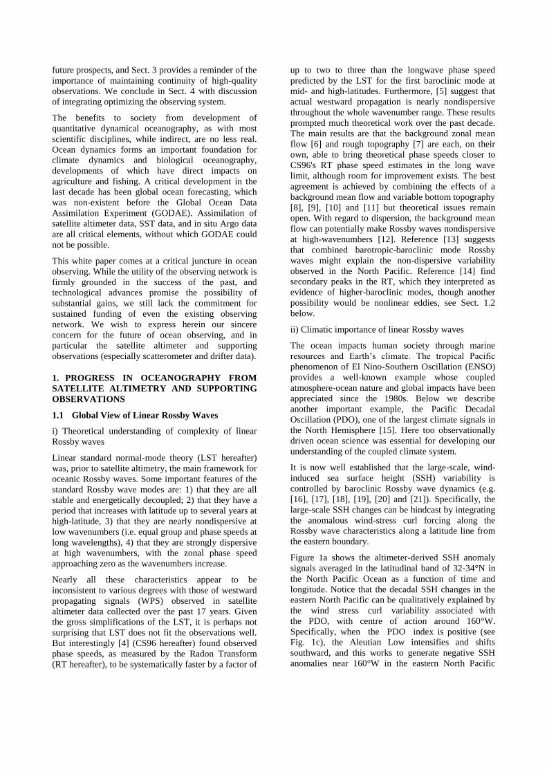
addition, a 'striped' global pattern of new jet-like

features ('striations') was unveiled and validated using

hydrographic data [39] (Fig. 3, below). While the

nature and significance of these striations is not

understood yet, the east-west tilt of the striations

suggests stationary waves. Striations are also found in

the altimetric sea level anomaly [40] which interact

with eddies as strongly as the 'mean' striations. Eddies

generated and moving along preferred paths may be

involved [41] and [42] but this remains controversial

[43].

Reference [41] studied the anisotropy of the most

energetic length scales, that are partially resolved by

the high resolution sea surface height anomaly data

from the constellation of at least three simultaneous

satellite altimeters monitoring most of the ocean from

year 2000 through 2005. They found mesoscale

structure in the difference between the eastward and

northward velocity variance throughout the

extratropical World Ocean, qualitatively consistent

with earlier results in the Southern Ocean [44]. The

velocity variance structures are within the range of

highly nonlinear eddy-eddy interactions. Contrary to

the standard nonlinear model of the ocean mesocale as

homogenous quasigeostrophic turbulence (e.g. [45])

the structures persist for years, i.e. much longer than

the inherent timescales of quasigeostrophic turbulence.

The pattern in velocity variance structures suggests an

organizing mechanism yet the patterns are not simply

related to bathymetry. The most important implications

are likely to be the spatially variable and strongly

anisotropic dispersion of traces. Climate models may

have to resolve the mesoscale explicitly since

dispersion parameterization is likely a more formidable

challenge than previously appreciated.

iii) Quantifying nonlinear interactions

In the mesoscale, the flow becomes nonlinear and more

complex, and theoretical models only make predictions

for statistical flow properties. One of the most

fundamental predictions is the so-called inverse energy

cascade, in which the large-scale flow gains energy

from smaller scales via quasi-2D nonlinear interaction

(e.g. [46]). The rate of this inverse cascade, called the

spectral kinetic energy flux, was diagnosed as a

function of length scale using multisatellite altimeter

data, revealing a universal shape over the South Pacific

that shifted to larger length scales closer to the Equator

[36]. Later analysis confirmed this universal shape

throughout the World Ocean, see Fig. 4 below. The

spectral flux divergence near the deformation radius

suggested baroclinic instability near the deformation

radius. This interpretation was later confirmed by

comparing the regions of horizontal 2D wavenumber

space that are baroclinically unstable, as computed

with climatological temperature and salinity data, and

with spectral flux measurements computed with

altimeter data [47]. These analyses provide the first

observational evidence of the importance of beta

(resulting from Earth‘s rotation and curvature) in

redirecting the inverse cascade, as anticipated by [25]

and clarified by [48] and [49].

While the spectral flux measurements were inspired by

classical quasi-2D turbulence theory, their observations

required some theoretical developments for consistent

interpretation. Classical theory predicts an inverse

cascade for the barotropic (depth averaged) flow only,

yet analysis of over 100 deep-water, long term, moored

current meters spanning the water column suggests that

most of the surface flow represents first mode

baroclinic motions (vertically sheared flows with

strongest signals in the upper ocean) [50]. Thus the

inverse cascade seen in altimeter data must imply an

inverse cascade of baroclinic KE, a novel idea

confirmed with idealized model simulations [51].

Figure 3: (a) 1993-2002 mean zonal surface geostrophic velocity calculated from the MDOT [37] high-pass filtered

with a two-dimensional Hanning filter of 4° half-width. (b) Ensemble-mean zonal velocity calculated from the data of

AOML. Rectangles in (a) outline two study domains where striations are validated by historical XBT data. Units are

cm/s. (Figure from [39].)

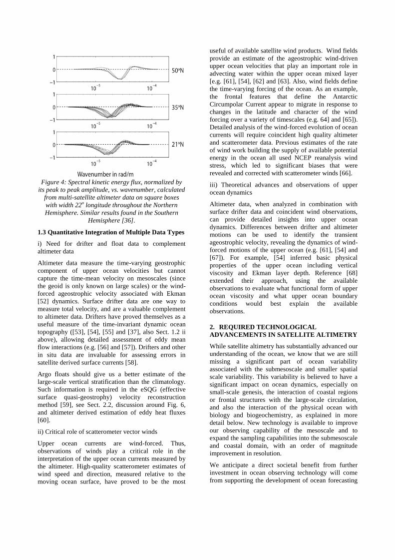
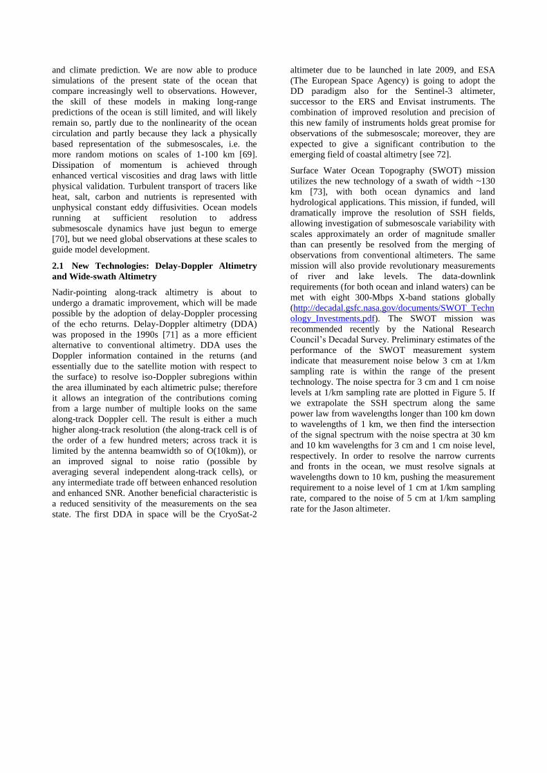
Figure 4: Spectral kinetic energy flux, normalized by

its peak to peak amplitude, vs. wavenumber, calculated

from multi-satellite altimeter data on square boxes

with width 22o longitude throughout the Northern

Hemisphere. Similar results found in the Southern

Hemisphere [36].

1.3 Quantitative Integration of Multiple Data Types

i) Need for drifter and float data to complement

altimeter data

Altimeter data measure the time-varying geostrophic

component of upper ocean velocities but cannot

capture the time-mean velocity on mesoscales (since

the geoid is only known on large scales) or the wind-

forced ageostrophic velocity associated with Ekman

[52] dynamics. Surface drifter data are one way to

measure total velocity, and are a valuable complement

to altimeter data. Drifters have proved themselves as a

useful measure of the time-invariant dynamic ocean

topography ([53], [54], [55] and [37], also Sect. 1.2 ii

above), allowing detailed assessment of eddy mean

flow interactions (e.g. [56] and [57]). Drifters and other

in situ data are invaluable for assessing errors in

satellite derived surface currents [58].

Argo floats should give us a better estimate of the

large-scale vertical stratification than the climatology.

Such information is required in the eSQG (effective

surface quasi-geostrophy) velocity reconstruction

method [59], see Sect. 2.2, discussion around Fig. 6,

and altimeter derived estimation of eddy heat fluxes

[60].

ii) Critical role of scatterometer vector winds

Upper ocean currents are wind-forced. Thus,

observations of winds play a critical role in the

interpretation of the upper ocean currents measured by

the altimeter. High-quality scatterometer estimates of

wind speed and direction, measured relative to the

moving ocean surface, have proved to be the most

useful of available satellite wind products. Wind fields

provide an estimate of the ageostrophic wind-driven

upper ocean velocities that play an important role in

advecting water within the upper ocean mixed layer

[e.g. [61], [54], [62] and [63]. Also, wind fields define

the time-varying forcing of the ocean. As an example,

the frontal features that define the Antarctic

Circumpolar Current appear to migrate in response to

changes in the latitude and character of the wind

forcing over a variety of timescales (e.g. 64] and [65]).

Detailed analysis of the wind-forced evolution of ocean

currents will require coincident high quality altimeter

and scatterometer data. Previous estimates of the rate

of wind work building the supply of available potential

energy in the ocean all used NCEP reanalysis wind

stress, which led to significant biases that were

revealed and corrected with scatterometer winds [66].

iii) Theoretical advances and observations of upper

ocean dynamics

Altimeter data, when analyzed in combination with

surface drifter data and coincident wind observations,

can provide detailed insights into upper ocean

dynamics. Differences between drifter and altimeter

motions can be used to identify the transient

ageostrophic velocity, revealing the dynamics of wind-

forced motions of the upper ocean (e.g. [61], [54] and

[67]). For example, [54] inferred basic physical

properties of the upper ocean including vertical

viscosity and Ekman layer depth. Reference [68]

extended their approach, using the available

observations to evaluate what functional form of upper

ocean viscosity and what upper ocean boundary

conditions would best explain the available

observations.

2. REQUIRED TECHNOLOGICAL

ADVANCEMENTS IN SATELLITE ALTIMETRY

While satellite altimetry has substantially advanced our

understanding of the ocean, we know that we are still

missing a significant part of ocean variability

associated with the submesoscale and smaller spatial

scale variability. This variability is believed to have a

significant impact on ocean dynamics, especially on

small-scale genesis, the interaction of coastal regions

or frontal structures with the large-scale circulation,

and also the interaction of the physical ocean with

biology and biogeochemistry, as explained in more

detail below. New technology is available to improve

our observing capability of the mesoscale and to

expand the sampling capabilities into the submesoscale

and coastal domain, with an order of magnitude

improvement in resolution.

We anticipate a direct societal benefit from further

investment in ocean observing technology will come

from supporting the development of ocean forecasting

and climate prediction. We are now able to produce

simulations of the present state of the ocean that

compare increasingly well to observations. However,

the skill of these models in making long-range

predictions of the ocean is still limited, and will likely

remain so, partly due to the nonlinearity of the ocean

circulation and partly because they lack a physically

based representation of the submesoscales, i.e. the

more random motions on scales of 1-100 km [69].

Dissipation of momentum is achieved through

enhanced vertical viscosities and drag laws with little

physical validation. Turbulent transport of tracers like

heat, salt, carbon and nutrients is represented with

unphysical constant eddy diffusivities. Ocean models

running at sufficient resolution to address

submesoscale dynamics have just begun to emerge

[70], but we need global observations at these scales to

guide model development.

2.1 New Technologies: Delay-Doppler Altimetry

and Wide-swath Altimetry

Nadir-pointing along-track altimetry is about to

undergo a dramatic improvement, which will be made

possible by the adoption of delay-Doppler processing

of the echo returns. Delay-Doppler altimetry (DDA)

was proposed in the 1990s [71] as a more efficient

alternative to conventional altimetry. DDA uses the

Doppler information contained in the returns (and

essentially due to the satellite motion with respect to

the surface) to resolve iso-Doppler subregions within

the area illuminated by each altimetric pulse; therefore

it allows an integration of the contributions coming

from a large number of multiple looks on the same

along-track Doppler cell. The result is either a much

higher along-track resolution (the along-track cell is of

the order of a few hundred meters; across track it is

limited by the antenna beamwidth so of O(10km)), or

an improved signal to noise ratio (possible by

averaging several independent along-track cells), or

any intermediate trade off between enhanced resolution

and enhanced SNR. Another beneficial characteristic is

a reduced sensitivity of the measurements on the sea

state. The first DDA in space will be the CryoSat-2

altimeter due to be launched in late 2009, and ESA

(The European Space Agency) is going to adopt the

DD paradigm also for the Sentinel-3 altimeter,

successor to the ERS and Envisat instruments. The

combination of improved resolution and precision of

this new family of instruments holds great promise for

observations of the submesoscale; moreover, they are

expected to give a significant contribution to the

emerging field of coastal altimetry [see 72].

Surface Water Ocean Topography (SWOT) mission

utilizes the new technology of a swath of width ~130

km [73], with both ocean dynamics and land

hydrological applications. This mission, if funded, will

dramatically improve the resolution of SSH fields,

allowing investigation of submesoscale variability with

scales approximately an order of magnitude smaller

than can presently be resolved from the merging of

observations from conventional altimeters. The same

mission will also provide revolutionary measurements

of river and lake levels. The data-downlink

requirements (for both ocean and inland waters) can be

met with eight 300-Mbps X-band stations globally

(http://decadal.gsfc.nasa.gov/documents/SWOT_Techn

ology_Investments.pdf). The SWOT mission was

recommended recently by the National Research

Council‘s Decadal Survey. Preliminary estimates of the

performance of the SWOT measurement system

indicate that measurement noise below 3 cm at 1/km

sampling rate is within the range of the present

technology. The noise spectra for 3 cm and 1 cm noise

levels at 1/km sampling rate are plotted in Figure 5. If

we extrapolate the SSH spectrum along the same

power law from wavelengths longer than 100 km down

to wavelengths of 1 km, we then find the intersection

of the signal spectrum with the noise spectra at 30 km

and 10 km wavelengths for 3 cm and 1 cm noise level,

respectively. In order to resolve the narrow currents

and fronts in the ocean, we must resolve signals at

wavelengths down to 10 km, pushing the measurement

requirement to a noise level of 1 cm at 1/km sampling

rate, compared to the noise of 5 cm at 1/km sampling

rate for the Jason altimeter.

Figure 5: Wavenumber spectrum of sea surface height anomaly from 147 repeat measurements along Jason pass 132

(solid line). The two slanted dashed lines represent two spectral power laws with k denote wavenumber. The two

horizontal dashed lines represent two levels of measurement noise at 1/km sampling rate: 3 cm and 1 cm. The slanting

solid straight line represents a linear fit of the spectrum in the range between 0.002 and 0.01 cycles/km. It intersects

with the two noise level lines at 30 km and 10 km wavelengths.

This performance in SSH measurement translates to a

geostrophic velocity error of 3 cm/sec at 10 km

wavelength at 45° latitude. The two dimensional SSH

map from SWOT will observe these features and will

thereby allow the study of the submesoscale ocean

eddies, fronts, narrow currents, and even the vertical

velocity at these scales. However, to capture related

temporal variability one would still need more than one

SWOT mission.

Despite the promise of the SWOT mission, we

speculate

that grappling with the following issues

could maximize the benefit of the mission:

Error statistics confronting effective use of SAR

altimetry will change across the swath due to the

change in resolving capability of an interferometer.

Are error statistics also isotropic in such data?

How relevant are assumptions about constant e-m

bias etc. with coherent altimeter systems?

Data assimilation of 2d interferometrically-derived

heights will have to be accompanied by some kind

We thank an anonymous reviewer for suggesting

these areas.

of 2d height error covariance functions in order to

assimilate the data, which is not a trivial issue.

2.2 Potential breakthroughs in ocean dynamics

and biogeochemistry

Global observations of the oceanic submesoscale are

essential to quantifying the ocean uptake of climate

relevant tracers such as heat and carbon. Traditional

altimeters revealed the fundamental role of mesoscale

eddies in the horizontal transport of tracers. Recent

theoretical work suggests that submesoscale motions

play a leading role in the vertical transport [74], [75],

[70] and [76]. Vertical velocities in the ocean require

higher spatial resolution because they result from

convergences and divergences in the horizontal

velocity field. Submesoscale motions at the ocean

surface are a superposition of Ekman velocities driven

by the wind, geostrophic velocities modified by finite

Rossby number dynamics. Scatterometers provide

detailed measurements of the wind stress field and

allow estimates of the wind-driven vertical velocities.

First attempts [77] and [78] to reconstruct the 3D

circulation in the upper 300m from climatological data

and high-resolution SST are quite promising. However

the high resolution SSH of wide-swath interferometry

is necessary to bring the approach to full fruition and

provide global maps of the vertical velocities

associated with geostrophic motions. Our

understanding of the ocean and its role in climate

would be radically advanced should such maps become

available. One first step in that direction will be the

availability of high-resolution (1-D) delay-Doppler

altimetry together with 2-D SST and ocean colour

fields made possible by Sentinel-3.

Attempts to further diagnose the oceanic circulation in

a realistic situation involving a mesoscale eddy field

with large Rossby numbers and an active mixed-layer

forced by high frequency winds have been recently

achieved [59]. Results (see Fig. 6) reveal that, despite

the presence of energetic near-inertial motions, a

snapshot of high resolution SSH allows reconstruction

of low frequency motions, including the vertical

velocities, for scales between 400km and 20km and

depths between the mixed-layer base and 500m. As

such these results highlight the potential of high-

resolution SSH to assess in the upper ocean the low

frequency horizontal and vertical fluxes of momentum

and tracers driven by mesoscale and submesoscale

dynamics. Some work still to be done to improve this

simple diagnosis method including its testing in a

broader range of mesoscale eddy and mixed-layer

regimes and its improvement to diagnose the specific

mixed-layer dynamics.

Figure 6: a) Observed low-frequency vertical velocity (in colors) and relative vorticity (contours) at 200 m. b) eSQG

reconstructed vertical velocities(in colors) and relative vorticity (contours) at 200 m. c) Correlation between observed

and eSQG reconstructed vertical velocities (blue line) and relative vorticity (red line). d) Vertical velocities RMS (Root-

Mean-Square) (blue) and relative vorticity RMS (red) observed in the PE simulation (solid line) and reconstructed

using eSQG (dashed line). Figure from [59].

The uptake of heat and carbon by the ocean is complete

only after these properties are transported away from the

surface turbulent boundary layer into the ocean interior.

Vertical velocities associated with divergences and

convergences of geostrophically balanced velocities on

10 km scale penetrate down to a few hundred meters

below the ocean surface [74]. Hence, the resolution of

delay-Doppler altimeters and SWOT will allow one to

compute the exchange of properties between the ocean

surface boundary layers and the interior. Furthermore,

these measurements will be fundamental to improving

the skills of coupled climate models that are very

sensitive to the exchange of properties between the

ocean and the atmosphere.

Other applications of the 1-D and 2-D SSH

measurements at the submesoscale are for estimates of

biological productivity. Ocean colour is very often

characterized by a web of filaments of enhanced

biological activity. It is impossible from a surface

picture to determine whether these filaments are

associated with lateral stirring of biomass or with new

productivity resulting from vertical advection of new

nutrients into the filaments. The distinction is crucial for

the global carbon cycle; the latter case implies an

enhancement of the biological carbon pump. Therefore,

delay-Doppler and wide-swath missions could

contribute essential new information to further our

understanding of the submesoscale physics and biology

of the upper ocean.

3. INTEGRATING EMERGING

TECHNOLOGIES WHILE MAINTAINING

EXISTING TECHNOLOGIES

Most climate records have been obtained as the by-

product of measurements made for a different purpose,

especially weather observations, and commonly it is

asserted that simply sustaining these networks is the

surest way to determining changes in climate. This

approach often generates some very great and

intractable difficulties. By some arguments, the

sustenance of high quality, sometimes demanding, but

nonetheless routine, measurements are the most difficult

of all to obtain and for many reasons. Each

oceanographic data type is in need of constant

supervision by technically qualified scientists who can

determine if standards are being followed, that

calibration protocols have been adhered to, and is in a

position to influence a decision to change a data type.

Because the intellectual payoff of many records might

be decades in the future, incentives have to be provided

for scientists to invest their time and energies into

efforts with little personal gratification other than a

sense of doing a service to the community.

Many examples of difficult decisions about technology

change abound. Therefore, given those experiences, we

should continue TOPEX-Jason class altimeters even

though the next generation of altimeters will have swath

capabilities. (Note that there remain calibration

discrepancies between radar altimeters.) Only if we can

assume the indefinite existence of high-quality

altimeters, the tide gauge network could be thinned. On

the other hand, in situ data are essential for calibrating

data from individual altimeter missions. In addition, sea

level has proven to vary on small coastal scale and to

monitor sea level changes we might even need to

expand the existing tide gauge network. Argo floats

should be redesigned to reach the sea floor.

Investigations should be carried out to determine

whether the surface observing system could be reduced ,

but at this point no indication exists that the ocean is

oversampled – just the opposite. In the same vein, we

need to investigate whether scatterometers should

completely replace the surface anemometer network

apart from a few very high quality calibration positions.

These questions will need to be answered before we can

decide what kind of investment should be made in

meteorological buoys. These are difficult problems that

cannot be relegated to uninterested committees for

solution. To answer them requires a serious and

quantitative design study of the observing system,

which addresses also uncertainties in the observations,

the models and the estimates that we obtain by bringing

observations and models together. An ocean observing

system that is intended to truly address climate change

must have a scientific supporting infrastructure that is in

constant control of the system.

4. INTEGRATING AND OPTIMIZING THE

GLOBAL OBSERVING SYSTEM: THE GREAT

CHALLENGE FOR COMING DECADES

Ocean data assimilation provides an objective way of

combining observational data on multiple variables in a

dynamically consistent framework, and forms the

backbone of ocean state estimation and ocean weather

forecasting. The most direct societal benefits from

ocean observations will come from the forecasting of

the ocean state, which impacts ship routing, weather

forecasting, the marine resources industry, etc. A great

challenge for the coming decade is the coordination of

ocean observations to optimize ocean state estimation

and forecasting through data assimilation. The altimeter

community in particular will need to coordinate with the

ocean modeling community to devise experiments to

determine what combination of satellites in which

orbits, carrying what combination of sensors

(conventional, delayed Doppler, swath) will have the

greatest impact on ocean state estimation and

forecasting. These are complex questions. Experience

from preliminary studies underway suggests that

ultimate decisions may involve subjective choices of

goals (e.g. large scale or mesoscale? surface or

barotropic? currents or transports?) and metrics to

decide which forecast is best.

While the needs of data assimilation provide a unique

method to guide resource development, we emphasize

that better forecasts are not the only consideration. The

dynamics of the ocean and its interaction with marine

biology and Earth‘s climate remain basic research areas,

and the immediate benefits are less clear, but the long-

term rewards may be most revolutionary. Basic research

may call for resources distinct from operational

oceanography. For example the highly nonlinear

submesoscale SSH field from SWOT might not benefit

data assimilation in present generation OGCMs (Ocean

General Circulation Models), but might provide crucial

information for understanding mixed layer biological

interactions.

The optimized system will likely include the

constellation of satellites that optimize operational

oceanography for some compromise set of criteria, and

some exploratory missions that push the frontiers of

basic science. We anticipate that SWOT and delayed

Doppler altimeters will form key components of a

constellation of altimeters.

5. REFERENCES

1. Fu, L.-L., and A. Cazenave, editors, (2001): Satellite

Altimetry and Earth Sciences: A Handbook of

Techniques and Applications, Academic Press, San

Diego, 463 pp.

2. Stammer, (1997): Global characteristics of ocean

variability estimated from regional TOPEX/POSEIDON

altimeter measurements, J. Phys. Oceanogr., 27, 1743–

1769.

3. Smith, R.D., Maltrud, M.E., Bryan, F.O., and Hecht,

M.W., (2000): Numerical simulation of the North

Atlantic ocean at 1/10°. J. Phys. Oceanogr., 30, 7,

1532–1561.

4. Chelton DB and Schlax MG, (1996): Global observations

of oceanic Rossby waves, Science, Volume: 272 Issue:

5259, Pages: 234-238.

5. Fu LL and Chelton DB (2001): Large-scale Ocean

circulation. In ``Satellite altimetry and Earth Sciences'',

Fu and Cazenave editors, International Geophysics

Series. Volume 69. Pages: 133-165

6. Killworth PD, Chelton DB, de Szoeke RA, (1997): The

speed of observed and theoretical long extratropical

planetary waves. J. Phys. Oceanogr. Volume: 27, Issue:

9, Pages: 1946-1966.

7. Tailleux R and McWilliams, JC, (2001): The effect of

bottom pressure decoupling on the speed of

extratropical, baroclinic Rossby waves. J. Phys.

Oceanogr. Volume: 31, Issue: 6, Pages: 1461-1476

8. Killworth PD and Blundell JR, (2003a): Long

extratropical planetary wave propagation in the presence

of slowly varying mean flow and bottom topography.

Part I: The local problem. J. Phys. Oceanogr. Volume:

33, Issue: 4, Pages: 784-801.

9. Killworth PD and Blundell JR, (2003b): Long

extratropical planetary wave propagation in the presence

of slowly varying mean flow and bottom topography.

Part II: Ray propagation and comparison with

observations. J. Phys. Oceanogr. Volume: 33, Issue: 4,

Pages: 802-821.

10. Killworth PD and Blundell JR, (2004): The dispersion

relation for planetary waves in the presence of mean

flow and topography. Part I: Analytical theory and one-

dimensional examples. J. Phys. Oceanogr. Volume: 34,

Issue: 12, Pages: 2692-2711.

11. Killworth PD and Blundell JR, (2005): The dispersion

relation for planetary waves in the presence of mean

flow and topography. Part II: Two-dimensional

examples and global results. J. Phys. Oceanogr.

Volume: 35, Issue: 11, Pages: 2110-2133.

12. Tailleux R and Maharaj AM, (2009): On the zonal

wavenumber/frequency spectrum of westward

propagation. Part I: Theory. To be submitted.

13. Wunsch, C. (2009): The Oceanic Variability Spectrum and

Transport Trends, Atmosphere-Ocean, 47(4), 281-291,

doi:10.3137/OC310.2009.

14. Maharaj AM, Holbrook NJ, and Cipollini, P (2009): An

assessment of multiple westward propagating signals in

sea level anomalies. Submitted to J. Geophys. Res. -

Oceans, 114, (C12016) pp. 1-14.

doi:10.1029/2008JC004799

15. Mantua, N. J., S. R. Hare, Y. Zhang, J. M. Wallace and R.

C. Francis (1997): A Pacific interdecadal climate

oscillation with impacts on salmon production. Bull.

Amer. Meteor. Soc., 78, 1069–1079.

16. Miller, A. J., D. R. Cayan, and W. B. White, (1998): A

westward intensified decadal change in the North Pacific

thermocline and gyre-scale circulation. J. Clim., 11,

3112–3127.

17. Deser, Clara, Michael A. Alexander And Michael S.

Timlin, (1999): Evidence for a Wind-Driven

Intensification of the Kuroshio Current Extension from

the 1970s to the 1980s , J. Clim., Vol. 12, pp. 1697—

1706.

18. Seager, R., Y. Kushnir, N. H. Naik, M. A. Cane, and J.

Miller, (2001): Wind-driven shifts in the latitude of the

Kuroshio–Oyashio extension and generation of SST

anomalies on decadal timescales. J. Clim., 14, 4249–

4265.

19. Schneider, N., A. J. Miller, and D. W. Pierce, (2002):

Anatomy of North Pacific decadal variability. J. Clim.,

586–605.

20. Qiu, B. and S. Chen (2005b): Variability of the Kuroshio

Extension Jet, Recirculation Gyre, and Mesoscale

Eddies on Decadal Time Scales, J. Phys. Oceanogr.,

Vol. 35, pp. 2090—2103.

21. Taguchi et al. Decadal Variability of the Kuroshio

Extension, (2007): Observations and an Eddy-Resolving

Model Hindcast, J. Clim. Vol. 20, pp. 2357—2377.

22. Kistler, R. E., Kalnay, E. M. W. Collins, S. Saha, G.

White, J. Woollen, M. Chelliah, W. Ebisuzaki, M.

Canamitsu, V. Kousky, H. van den Dool, R. Jenne and

M. Fiorinio, (2001): The NCEP/NCAR 50-year

reanalysis: Monthly means CD-ROM and

documentation, Bull. Amer. Met. Soc, Vol. 82, pp. 247—

267.

23. Lorenz, E. (1963): Deterministic nonperiodic flow, J.

Atmos. Sci., Vol. 20, pp. 130—141.

24. Charney, J.G. (1971): Geostrophic Turbulence, J. Atmos.

Sci. Vol. 28, pp. 1087—1095.

25. Rhines, P. (1975): Waves and turbulence on a beta-plane,

J. Fluid Mech., Vol. 69, pp. 417—443.

26. McWilliams, J. C., and G. R. Flierl (1979): On the

evolution of isolated, nonlinear vortices, J. Phys.

Oceanogr., 9, 1155-1182.

27. Salmon, R. (1980): Baroclinic Instability And Geostrophic

Turbulence, Geophys. Astrophys. Fluid Dyn., Vol. 15,

pp. 167—211.

28. Hua, B.L. and Haidvogel, D. (1986): Numerical

simulations of the vertical structure of quasi-geostrophic

turbulence, J. Atmos. Sci., Vol. 43, pp. 2923—2936.

29. Treguier, A. and L. Panetta, (1994): Multiple Zonal Jets in

a Quasigeostrophic Model of the Antarctic Circumpolar

Current, J. Phys. Oceanogr., Vol. 24, pp. 2263—2277.

30. Jiang, S., F. Jin and M. Ghil, (1995): Multiple equilibria,

Periodic and Aperiodic solutions in a wind-driven,

double-gyre, shallow-water model, J. Phys. Oceanogr.,

Vol. 25, pp. 764—786.

31. Chelton, D.B. and Schlax, M.G. (2003): The accuracies of

smoothed sea surface height fields constructed from

tandem satellite altimeter datasets, J. Atmos. Oceanic

Technol., Vol. 20, pp. 1276—1302.

32. Ducet, N., P.-Y. Le Traon, and G. Reverdin, (2000):

Global high resolution mapping of ocean circulation

from TOPEX/POSEIDON and ERS-1/2. J. Geophys.

Res., 105, 19,477-19,498.

33. Pascual, A., Faugere, Y., G. Larnicol, P.Y. Le Traon,

(2006): Improved description of the ocean mesoscale

variability by combining four satellite altimeters.

Geophys. Res. Letters, 33 (2): Art. No. L02611.

34. Chelton, D. B., M. G. Schlax, R. M. Samelson, and R. A.

de Szoeke, (2007): Global observations of large oceanic

eddies. Geophys. Res. Lett., 34, L15606,

doi:10.1029/2007GL030812.

35. Tulloch, R. and J. Marshall and K. S. Smith: (2009):

Interpretation of the propagation of surface altimetric

observations in terms of planetary waves and

geostrophic turbulence, J. Geophys. Res. Oceans, Vol.

114, doi:10.1029/2008JC005055.

36. Scott, R.B. and F. Wang (2005): Direct evidence of an

oceanic inverse kinetic energy cascade from satellite

altimetry, J. Phys. Oceanogr, Vol. 35, pp. 1650—166.

37. Maximenko, N.A., and P.P. Niiler, (2005): Hybrid decade-

mean global sea level with mesoscale resolution. In N.

Saxena (Ed.) Recent Advances in Marine Science and

Technology, (2004), pp. 55-59. Honolulu: PACON

International.

38. Maximenko, N., P. Niiler, M.-H. Rio, O. Melnichenko, L.

Centurioni, D. Chambers, V. Zlotnicki, and B. Galperin,

(2009): Mean dynamic topography of the ocean derived

from satellite and drifting buoy data using three different

techniques. (2009): J. Atmos. Oceanic Technol., Vol. 26,

pp. 1910--1919.

39. Maximenko, N.A., O. V. Melnichenko, P. P. Niiler, and H.

Sasaki, (2008): Stationary mesoscale jet-like features in

the ocean. (2008): Geophys. Res. Lett., 35, L08603,

doi:10.1029/2008GL033267.

40. Maximenko, N.A., B. Bang, and H. Sasaki, (2005):

Observational evidence of alternating zonal jets in the

World Ocean. Geophys. Res. Lett., 32, L12607,

doi:10.1029/2005GL022728.

41. Scott, R.B., Arbic, B.K., Holland, C.L., Sen, A., and Qiu,

B. (2008): Zonal versus meridional velocity variance in

satellite observations and realistic and idealized ocean

circulation models, Ocean Modelling, Vol. 23, pp.

102—112.

42. Schlax, Michael G. and Dudley B. Chelton, (2008): The

influence of mesoscale eddies on the detection of quasi-

zonal jets in the ocean, Geophys. Res. Lett., VOL. 35,

L24602, doi:10.1029/2008GL035998.

43. Maximenko, N. A., O. V. Melnichenko, and H.-P. Huang,

(2009): Are oceanic striations an artefact of moving

eddies? In prep.

44. Morrow, R.A., R. Coleman, J.A Church, and D.B.

Chelton, (1994): Surface eddy momentum flux and

velocity variances in the Southern Ocean from Geosat

altimetry. J. Phys. Oceanogr., 24, 2050-2071.

45. Arbic, B.K. and Flierl, G.R. (2004): Effects of mean flow

direction on energy, isotropy, and coherence of

baroclinically unstable beta-plane geostrophic

turbulence, J. Phys. Oceanogr., Vol. 34, pp. 77—93.

46. Charney, J.G. (1971): Geostrophic Turbulence, J. Atmos.

Sci. Vol. 28, pp. 1087—1095.

47. Qiu, B., R.B. Scott, and S. Chen, (2008): Length-scales of

generation and nonlinear evolution of the seaonally-

modulated South Pacific Subtropic Countercurrent, J.

Phys. Oceanogr., Vol. 38, pp. 1515—1528.

48. Vallis, G.K. and M. Maltrud, (1993): Generation of mean

flows and jets on a beta plane and over topography, J.

Phys. Oceanogr., Vol. 23, pp. 1346—1362.

49. Sukoriansky, S., N. Dikovskaya, and B. Galperin, (2007):

On the ‗arrest‘ of the inverse energy cascade and the

Rhines scale, J. Atmos. Sci., 64, 3312–3327.

50. Wunsch, C. (1997): The vertical partition of oceanic

horizontal kinetic energy and the spectrum of global

variability, J. Phys. Oceanogr., Vol.27, pp. 1770—1794.

51. Scott, R.B. and B.K. Arbic (2007): Spectral energy fluxes

in geostrophic turbulence: implications for ocean

energetic, J. Phys. Oceanogr, Vol. 37, pp. 673—688.

52. Ekman, V.W. (1905): On the influence of the earth's

rotation on ocean currents. Ark. Mat. Astron. Fys. 2 (11):

1-52.

53. Niiler, P. P. and N. A. Maximenko and J. C. McWilliams,

(2003): Dynamically balanced absolute sea level of the

global ocean derived from near-surface velocity

observations, Geophys. Res. Lett., 30:22, 2164,

doi:10.1029/2003GL018628.

54. Rio, M.-H. and F. Hernandez, (2003): High frequency

response of wind-driven currents measured by drifting

buoys and altimetry over the world ocean, J. Geophys.

Res., 108(C8), 3283, doi:10.1029/2002JC001655.

55. Rio, M. H. and F. Hernandez, (2004): A mean dynamic

topography computed over the world ocean from

altimetry, in situ measurements, and a geoid model, J.

Geophys. Res., 109, C12032,

doi:10.1029/2003JC002226.

56. Hughes, C. W. and Ash E. R., (2001): Eddy forcing of the

mean flow in the Southern Ocean, J. Phys. Oceanogr.,

31(10), pp.2871-2885.

57. Hughes, C. W., (2005): Nonlinear vorticity balance of the

Antarctic Circumpolar Current, J. Geophys. Res., 110,

C11008, doi:10.1029/2004JC002753.

58. Johnson, E.S., F. Bonjean, G.S.E. Lagerloef, J.T. Gunn,

and G. T. Mitchum, (2007): Validation and Error

Analysis of OSCAR Sea-surface Currents, J. of Atmos.

Oceanic Technol., 24(4), 688-701.

59. Klein P., J. Isern-Fontanet, G. Lapeyre, G. Roullet, E.

Danioux, B. Chapron, S. LeGentil and H. Sasaki,

(2009): Diagnosis of vertical velocities in the upper

ocean from high resolution Sea Surface Height.

Geophys. Res. Lett., 36, L12603,

doi:10.1029/2009GL038359.

60. Qiu, B. and S. Chen (2005a): Eddy-Induced Heat

Transport in the Subtropical North Pacific from Argo,

TMI, and Altimetry Measurements, J. Phys. Oceanogr.,

Vol. 35, pp. 458—473.

61. Ralph, E. A. and P. P. Niiler, (1999): Wind-driven

currents in the tropical Pacific, J. Phys. Oceanogr., 29,

pp. 2121--2129.

62. Dong, S., S. T. Gille, J. Sprintall, (2007): An assessment

of the Southern Ocean mixed-layer heat budget, J. Clim.,

20, 4425-4442.

63. Bonjean, F., and G.S.E. Lagerloef, (2002): Diagnostic

model and analysis of the surface currents in the tropical

Pacific Ocean, J. Phys. Oceanogr., 32, 2938-2954.

64. Dong, S., J. Sprintall, and S. T. Gille, (2006): Location of

the Polar Front from AMSR-E satellite sea surface

temperature measurements, J. Phys. Oceanogr., 36,

2075-2089.

65. Sallée, J.-B., K. Speer, and R. Morrow, (2008): Southern

Ocean fronts and their variability to climate modes, J.

Clim., 21(12), 3020-3039.

66. Scott, R.B. and Xu, Y. (2009): An update on the wind

power input to the surface geostrophic flow of the World

Ocean, Deep Sea Research I, Vol. 56, pp. 295—304.

67. Elipot, S. and S. T. Gille, (2009a): Estimates of wind

energy input to the Ekman layer in the Southern Ocean

from surface drifter data, J. Geophys. Res., Vol. 114,

doi:10.1029/2008JC005170.

68. Elipot, S. and S. T. Gille, S. T., (2009b): Ekman layers in

the Southern Ocean: spectral models and observations,

vertical viscosity and boundary layer depth, submitted

Ocean Sci. Discuss., 6, 277-341.

69. Nature, editorial (2008): ―The next big climate challenge‖.

Nature, Vol. 453, Issue no. 7193, p. 257.

70. Capet, X., J.C. McWilliams, M.J. Molemaker, and A.F.

Shchepetkin, (2008): Mesoscale to submesoscale

transition in the California Current System. Part I: Flow

structure, eddy flux, and observational tests. J. Phys.

Oceanogr., Vol. 38, 29-43.

71. Raney, R. K., (1998): The delay Doppler radar altimeter,

IEEE Transactions on Geoscience and Remote Sensing,

vol. 36, pp. 1578-1588.

72. Cipollini, P. & Co-Authors (2010). "The Role of Altimetry

in Coastal Observing Systems" in these proceedings

(Vol. 2), doi:10.5270/OceanObs09.cwp.16.

73. Fu, L.-L., and R. Rodriguez, (2004): High-resolution

measurement of ocean surface topography by radar

interferometry for oceanographic and geophysical

applications, AGU Geophysical Monograph 150, IUGG

Vol. 19: "State of the Planet: Frontiers and Challenges",

R.S.J. Sparks and C.J. Hawkesworth, editors, 209-224.

74. Lapeyre, G., P. Klein, and B. L. Hua, (2006): Oceanic

restratification forced by surface frontogenesis. J. Phys.

Oceanogr., 36, 1577-1590.

75. Boccaletti G., R. Ferrari, and B. Fox-Kemper, (2007):

Mixed Layer Instabilities and Restratification, J. Phys.

Oceanogr., 37, 2228-2250.

76. Klein, P., Hua B.L., G. Lapeyre, X. Capet, S. LeGentil and

H. Sasaki., (2008): Upper Ocean Dynamics from High

3-D Resolution Simulations. J. Phys. Oceanogr., 38, pp.

1748–1763.

77. Lapeyre, G., and P. Klein, (2006): Dynamics of upper

oceanic layers in terms of surface quasigeostrophic

theory. J. Phys. Oceanogr., 36, 165-176.

78. LaCasce, J. H. and A. Mahedavan, (2006): Estimating

sub-surface horizontal and vertical velocity from sea

surface temperature. J. Mar. Res., 64, 695-721.