Improved Estimators of Mean of Sensitive

Variables using Optional RRT Models

Sat Gupta

Department of Mathematics and Statistics

University of North Carolina – Greensboro

sngupta@uncg.edu

University of South Florida

March 9, 2016

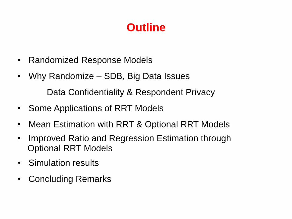
Outline

• Randomized Response Models

• Why Randomize – SDB, Big Data Issues

Data Confidentiality & Respondent Privacy

• Some Applications of RRT Models

• Mean Estimation with RRT & Optional RRT Models

• Improved Ratio and Regression Estimation through Optional RRT Models

• Simulation results

• Concluding Remarks

Detour

Math & Stats at

UNC Greensboro

Department of Mathematics and Statistics

Computational Mathematics Ph.D. Program

Areas of research include: • Combinatorics • Differential Equations • Functional Analysis • Group Theory • Statistics • Mathematical Biology • Number Theory • Numerical Analysis • Topology

MA in Mathematics Concentrations in • Mathematics • Applied Statistics • Actuarial Mathematics* • College Teaching* • Data Analytics* * From Spring 2016 (anticipated)

uncg.edu/mat

Our Graduate Assistants usually receive: $18,000 + tuition waivers for the Ph.D. Program in Computational Mathematics $10,800 + tuition waivers for the M.A. in Mathematics (Pure Mathematics, Applied Mathematics, Applied Statistics specialties) For more information, go to www.uncg.edu/mat or contact our Graduate Director, Dr. Gregory Bell at gcbell@uncg.edu.

Our Graduate students are usually funded via graduate assistantships. Their duties include one or a combination of the following: teaching lower level Mathematics or Statistics courses, tutoring in the Math Help Center, or monitoring the Math Emporium Lab. Additional summer funding is also available.

International Biennial Conference on Advances in Interdisciplinary

Statistics and Combinatorics

Student Activities

Pi Mu Epsilon Math Club

Graduate Tea

Student Publications Some of the Journals that feature student publications.

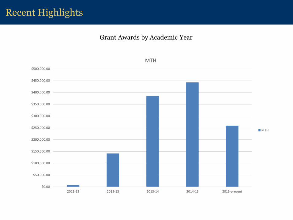
Recent Highlights

Grant Awards by Academic Year

$0.00

$50,000.00

$100,000.00

$150,000.00

$200,000.00

$250,000.00

$300,000.00

$350,000.00

$400,000.00

$450,000.00

$500,000.00

2011-12 2012-13 2013-14 2014-15 2015-present

MTH

MTH

Journals Associated with the Department

Dr. Sat Gupta serves as Editor-in-Chief

Dr. Jerry Vaughan serves as one of two Editors-in-Chief

Dr. Jan Rychtar and Sebastian Pauli serve as

Editors-in-Chief http://www.tandfonline.com/loi/UJSP20

http://www.journals.elsevier.com/topology-and-its-applications/

http://ncjms.uncg.edu/

Back to Business

Randomized Response Techniques –

RRT Models

• Introduced by Warner (1965) to decrease Social Desirability Bias.

• The respondents ‘randomize’ or ‘scramble’ the response to a sensitive or threatening question.

• Unscrambling can be done only at the group level, not at the individual level.

• Many Other Models – Greenberg Unrelated Question Model etc.

SDB – Social Desirability Response Bias

• Tendency in humans to look good in the face of

incriminating questions

• Sensitivity may result in refusal to answer, or

intentional false answers.

Getting Around SDB

• SDB Scale

• Bogus Pipeline

• RRT Models – But Privacy Protection is an Important

Issue

Types of RRT Models

• Binary vs. Multi-category vs. Quantitative

• Full RRT vs. Partial RRT Vs. Optional RRT

• Additive vs. Multiplicative vs. Generalized

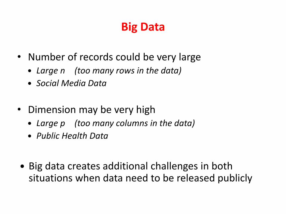
Big Data

• Number of records could be very large Large n (too many rows in the data)

Social Media Data

• Dimension may be very high Large p (too many columns in the data)

Public Health Data

Big data creates additional challenges in both

situations when data need to be released publicly

Why Release Data Publicly

• Advancement of science

• Student training

• Public interest

• Funding agencies may insist

Data Confidentiality – Back-End Problem

• Maintain confidentiality of record level data. Less worry at aggregate level

• Ethical/Legal Issues

• It is not enough to delete names/ subject ID’s

• Respondent safety and protection

Respondent Privacy – Front-End Problem

• SDB Related Issues

• Respondent Cooperation

Data Confidentiality & Respondent Privacy

• Too much scrambling (masking) or too little scrambling

• Think of two data scrambling models for variable X

Y= 𝑋 + 𝑆 Y= 𝑋 + θ 𝑆 S is a scrambling variable, θ is a constant

• Confidentiality is higher when θ is larger

• Data quality is better when θ is smaller

• Same dilemma as in confidence intervals

Some RRT Applications

Ostapczuk, Martin, Jochen Musch, and Morten Moshagen (2009):

A randomized-response investigation of the education effect in attitudes towards foreigners, European Journal of Social Psychology, 39 (6)

Spears- Gill, Tracy., Tuck, Anna., Gupta, Sat., Crowe, Mary., Jennifer Figuerova (2013):

A Field Test of Optional Unrelated Question Randomized Response Models – Estimates of Risky Sexual Behaviors, Springer Proceedings in Mathematics and Statistics, Vol. 64, 135-146

Education Effect in Attitudes Towards

Foreigners in Germany

• Under direct questioning conditions, 75% of the highly educated expressed xenophile attitudes, as opposed to only 55% of the less educated.

• Under randomized-response conditions, 53% xenophiles among the highly educated, and 24% among the less educated

Spears-Gill et al. (2013) - Field Test: Estimates of Risky Sexual Behaviors

Use of Greenberg Unrelated Question RRT Model Sensitive question Have you ever been told by a healthcare professional that you have a sexually transmitted disease(STD)?

Unrelated question Were you born between January 1st and October 31st?

Estimate of STD Prevalence

Method

95% CI

Optional RRT 0.0367 （0.0159, 0.0576）

Check Box Method

0.0900 （0.0438， 0.1362）

Face-to-face Interview

0.0200 (-0.0042， 0.0442)

Mean Estimators of Sensitive Variables

Eichhorn and Hayre (1983): Multiplicative Model

JSPI

• Y: Sensitive quantitative variable of interest with unknown

mean and an unknown variance of .

• S: Scrambling variable independent of Y with known mean of

and a known variance of .

The reported response Z is given by

This suggests estimating by where

Y2

Y

S

2

S

YSZ

Y Y

ZY

Gupta et al. (2002): Optional RRT Model JSPI

• Multiplicative optional RRT is used to scramble the response :

• The respondents provides a multiplicatively scrambled response for Y if they consider the question sensitive, and a true response otherwise.

• The response is given by:

where T is a Bernoulli random variable with parameter W and

S is a scrambling variable with unit mean and known variance, independent of Y

YSZ T

Mean Estimation

• An unbiased estimator of the population mean is given by

• Note that W is not involved in the unbiased estimation of .

• The relative efficiency of Gupta et al. (2002) estimator with respect

to the estimator of Eichhorn and Hayre (1983) is greater than or

equal to 1.

n

i

iY Zn 1

1

Y

Y

Sensitivity Estimation

• Taking Log and then expected values on both sides of

leads to an estimator of W given by

YSZ T

SE

Zn

Zn

W

n

i

n

i

ii

log

1loglog

1

ˆ 1 1

• Asymptotics a challenge with multiplicative

scrambling

• Split sample approach is an option

• Loss of anonymity

• Additive scrambling works better

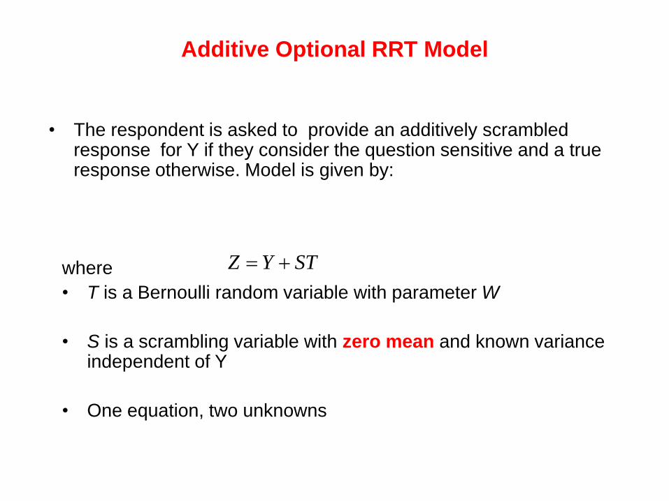
Additive Optional RRT Model

• The respondent is asked to provide an additively scrambled response for Y if they consider the question sensitive and a true response otherwise. Model is given by:

where

• T is a Bernoulli random variable with parameter W

• S is a scrambling variable with zero mean and known variance independent of Y

• One equation, two unknowns

STYZ

Estimation of the Mean

• An unbiased estimator of population mean is the sample mean of

the reported responses

• Note that is not involved in the unbiased estimation

of

n

i

iYW zn 1

1

W

YW

Additive Optional RRT Model Using Split Sample Approach

• Total sample size n is split into two independent sub-samples of

sizes and

• The mean and variance respectively for are and .

• The mean and variance respectively for are and .

• We assume that , and are mutually independent.

1n 2n

iS 2,1i i2

iS

Y

Y2

YY

2,1iS i

Estimation of Mean and Sensitivity Level

• The reported response in the sub- sample is given by

We note where .

It follows

and

iZthi

2,11

i

WyprobabilitwithSY

WyprobabilitwithYZ

i

i

WZE iYi 2,1 iSE ii

,

12

2112

ZEZEY

12

12

ZEZEW

Gupta et al. (2010): Unbiased Estimators of

Mean and Sensitivity Level - JSPI

• , ,

where respectively are the sample mean of reported responses

in the two sub-samples.

• The mean square error of is given by

where

12

2112ˆ

zzY 21

12

12ˆ

zzW

21

2

2

22

1

2

1

12

22

12

21

111ˆ

ZZYn

f

n

fMSE

N

nf 1

1 N

nf 2

2 21 ffN

nf

N

i

ZZ iZ

N 1

2

2

2

1

12

21 , zz

Y

Improvement through

Ratio and Regression Estimation

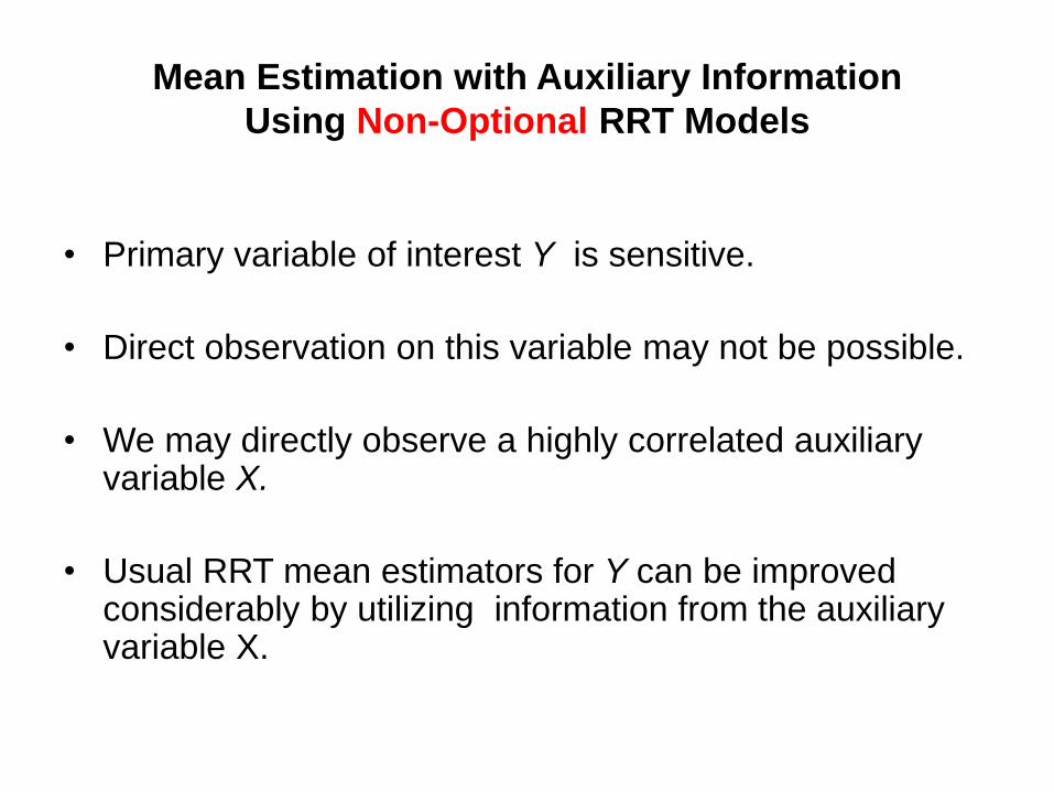
Mean Estimation with Auxiliary Information

Using Non-Optional RRT Models

• Primary variable of interest Y is sensitive.

• Direct observation on this variable may not be possible.

• We may directly observe a highly correlated auxiliary variable X.

• Usual RRT mean estimators for Y can be improved considerably by utilizing information from the auxiliary variable X.

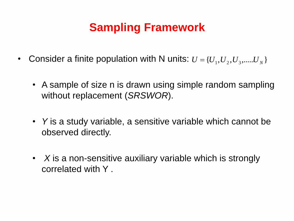
Sampling Framework

• Consider a finite population with N units:

• A sample of size n is drawn using simple random sampling

without replacement (SRSWOR).

• Y is a study variable, a sensitive variable which cannot be

observed directly.

• X is a non-sensitive auxiliary variable which is strongly

correlated with Y .

},.....,,{ 321 NUUUUU

Sousa et al. (2010): Improved Mean Estimators with Auxiliary Information - JSTP

Ratio Estimation Using Non-optional RRT Model

Sousa et al. (2010) proposed a non-optional ratio estimator for the

mean of sensitive variable Y utilizing information from a non- sensitive

auxiliary variable X. Their estimator is given by

In the above expression is the sample mean of reported responses

obtained from a non- optional additive RRT model.

xz X

AR

z

Gupta et al. (2012): Regression Estimator Using Non-Optional RRT Model - CIS-TM

• Gupta et al. (2012) proposed a non-optional regression estimator

for the mean of sensitive variable utilizing information from a non-

sensitive auxiliary variable .Their estimator is given by

• is the sample mean of reported responses obtained from a non

optional additive RRT model

• is the sample regression coefficient between and X.

xXz zxg ˆˆRe

X

Y

z

zx Z

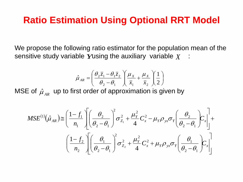
Ratio Estimation Using Optional RRT Model

We propose the following ratio estimator for the population mean of the

sensitive study variable using the auxiliary variable :

MSE of up to first order of approximation is given by

X

2

1ˆ

2112

2112

xx

zz XXAR

xYyxYxY

Z

xYyxYxY

ZAR

CCn

f

CCn

fMSE

12

122

2

2

12

1

2

2

12

222

2

2

12

2

1

11

4

1

4

1ˆ

2

1

AR

Y

Efficiency Comparison

• if with

where

YAR MSEMSE ˆˆ

4yx

2

2

1

1 11

n

f

n

f

12

1

2

2

12

2

1

1 11

n

f

n

f

yx CC

• Equal sub-sample sizes: ,

and hence .

In this case if

• Unequal sub-sample sizes:

We can choose scrambling variables and sample sizes in such a

way that and hence again

if

221 nnn

2

2

1

1 11

n

f

n

f

2

1

4

YAR MSEMSE ˆˆ 2

1yx

21 nn

2

1

4

YAR MSEMSE ˆˆ 2

1yx

• Note that under the following parameter choices which are

always possible :

• If both the scrambling variable means are strictly positive, then we associate the smaller mean with the smaller sub-sample

• If both the scrambling variable means are strictly negative, then we associate the smaller mean with the larger sub-sample.

• If the scrambling variable means are with opposite signs then we associate the one with the larger absolute value to the larger sub-sample.

• If one of the scrambling variable means is zero then we associate the smaller sub-sample size to the variable with mean zero.

2

1

4

• The ratio estimator is always more efficient than the

ordinary additive optional mean estimator if

.

and

• We see if .

YAR MSEMSE ˆˆ 5.0yx

5.0yx yx CC

AR

Y

Simulations

• We show the above conclusion with the following bivariate normal

population:

1000 iterations.

1,2,3,2,6,4,500021 SSYXYXN

500,5.05 12 n

Table 1: Estimates with Theoretical (bold) and

Empirical MSE’s ( )

0.3 0.35 5.8640 5.8688

0.0582 0.0400 0.35 5.8608 5.8695

0.0584 0.0623

0.0583 0.0580 0.0388 0.0585

0.5 0.55 5.8003 5.7979 0.0606 0.0425

0.55 5.790 5.7963 0.0609 0.0648

0.0694 0.0650 0.0474 0.0716

0.7 0.65 5.8923 5.8981 0.0629 0.0448

0.66 5.8983 5.901 0.0632 0.0671

0.0525 0.0366 0.0551 0.0603

0.8 0.81 5.8332 5.8340 0.0640 0.0458

0.80 5.8437 5.8502 0.0643 0.0681

0.0616 0.0435 0.0591 0.0617

0.9 0.92 5.8211 5.8264 0.0650 0.0468

0.92 5.8451 5.8461 0.0653 0.0691

0.0618 0.0445 0.0644 0.0660

200,300 12 nn

500,6 nY

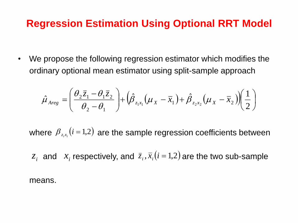
Regression Estimation Using Optional RRT Model

• We propose the following regression estimator which modifies the

ordinary optional mean estimator using split-sample approach

where are the sample regression coefficients between

and respectively, and are the two sub-sample

means.

2

1ˆˆˆ21

12

2112

2211xx

zzXxzXxzAreg

2,1iii xz

iz ix 2,1, ixz ii

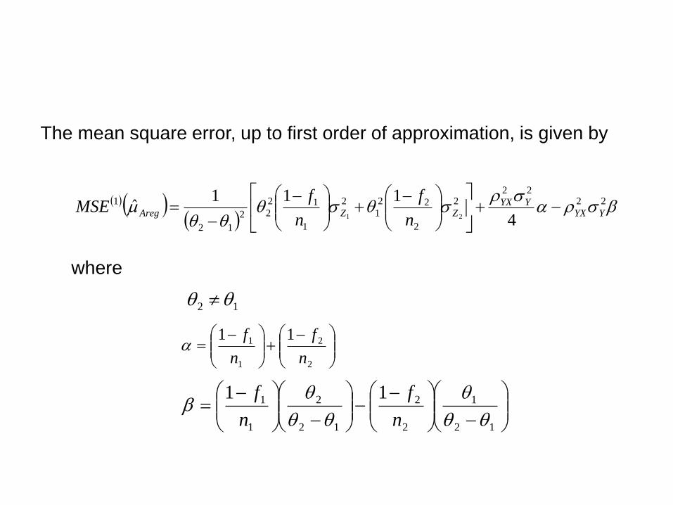
The mean square error, up to first order of approximation, is given by

where

2222

2

2

22

1

2

1

12

22

12

1

4

111ˆ

21 YYXYYX

ZZAregn

f

n

fMSE

12

2

2

1

1 11

n

f

n

f

12

1

2

2

12

2

1

1 11

n

f

n

f

Efficiency Comparison

We note

• if

• if

The above conditions can be achieved with proper choices

of sub-sample sizes and scrambling variables.

YAreg MSEMSE ˆˆ 14

ARAreg MSEMSE ˆˆ

4YX

xy CC

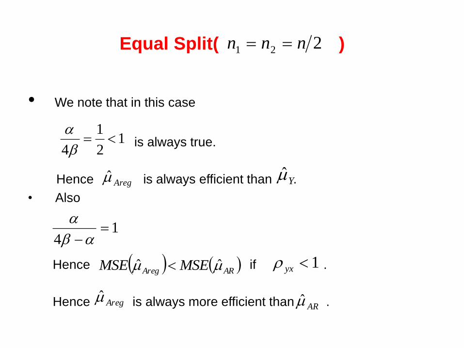
Equal Split( )

• We note that in this case

is always true.

Hence is always efficient than .

• Also

Hence if .

Hence is always more efficient than .

221 nnn

12

1

4

14

Areg

AR

Y

ARAreg MSEMSE ˆˆ 1yx

Areg

Simulations

• Consider a bivariate normal population with the following

characteristics:

1000 iterations

.1,2,3,2,6,4,500021 SSYXYXN

5.0,5 21

Table 2: Estimate with Theoretical(bold) and

Empirical MSE’s ( )

200 300 0.3 0.35 5.9061 5.9084 5.9046 0.0250 0.0190 0.0174

0.0231 0.0163 0.0178

200 300 0.5 0.53 5.8576 5.8590 5.8558 0.0256 0.0196 0.0180

0.0257 0.0196 0.0189

200 300 0.7 0.65 5.8638 5.8679 5.8642 0.0261 0.0201 0.0185

0.0253 0.0205 0.0189

200 300 0.8 0.77 5.8479 5.8549 5.8505 0.0262 0.0203 0.0187

0.0277 0.0212 0.0201

200 300 0.9 0.90 5.8418 5.8435 5.8400 0.0264 0.0204 0.0188

0.0292 0.0234 0.0223

6,8.0,500 Yyxn

Table 3: Estimate with theoretical(bold) and

Empirical MSE’s( )

200 300 0.3 0.3454 5.9164 5.9178 5.9155 0.0251 0.0336 0.0240

0.0230 0.0333 0.0227

200 300 0.5 0.5438 5.8582 5.8618 5.8580 0.0257 0.0342 0.0246

0.0276 0.0272 0.0366

200 300 0.7 0.6519 5.8746 5.8876 5.8773 0.0262 0.0347 0.0251

0.0251 0.0333 0.0242

200 300 0.8 0.7718 5.8611 5.8605 5.8597 0.0264 0.0349 0.0252

0.0349 0.0268 0.0261

200 300 0.9 0.9024 5.8455 5.8455 5.8442 0.0265 0.0350 0.0254

0.0291 0.0365 0.0282

6,3.0,500 Yyxn

Conclusions

• Even for small correlation between the study variable

and the auxiliary variable, the proposed regression

estimator is always more efficient than both the ratio

estimator and the ordinary RRT mean estimator.

• As seen in Table 2 , for the optional RRT mean

estimator is more efficient than the ratio estimator.

However, the proposed regression estimator is always

more efficient than both the additive ratio estimator and

the ordinary optional RRT mean estimator.

5.0yx

Conclusions

• As the sensitivity W increases, the

increase, highlighting the usefulness of an optional

RRT model since W is highest (equal to 1) for non-

optional model.

• Similar improvements possible In stratified sampling

also

sMSE '

THANK YOU