Embed Size (px)
Citation preview
SAS ODS Graphics and StatisticalGraphics Procedures
Mervyn Marasinghe
ODS graphics or template-based graphics
• ODS Graphicsd is currently the default for producing graphs in most SASstatistical procedures
• Thus ODS Graphics produced by various procedures appear automatically inthe output
• In SAS 9.2 under the SAS Windowing environment, ODS GRAPHICS ONstatement was required to enable ODS Graphics
• With ODS Graphics, styles and templates control the appearance of tables andgraphics
• SAS 9.3 uses the default style called HTMLBlue available for the HTML des-tination
• When statements that produce graphics are included in a proc step ODSGraphics produced will beoutput in HTML by default
• For e.g., the HISTOGRAM statement used in a proc univariate step will pro-duce ODS Graphics output in HTML
• As usual, graphical and other output (such as tables produced by the proce-dure) may be sent to a destination such as a pdf or an rtf file
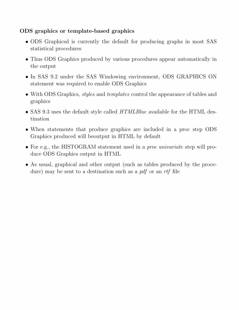
SAS Example C4
libname libc "U:\Documents\Stat479\";
data new;
set libc.biology;
BMI=703*Weight/Height**2;
run;
proc ttest data=new cochran ci=equal;
class Sex;
var BMI;
title "Biology class: Two Sample T-test";
run;
Figure 1: SAS Example C4: Output from PROC TTEST (Part 1)
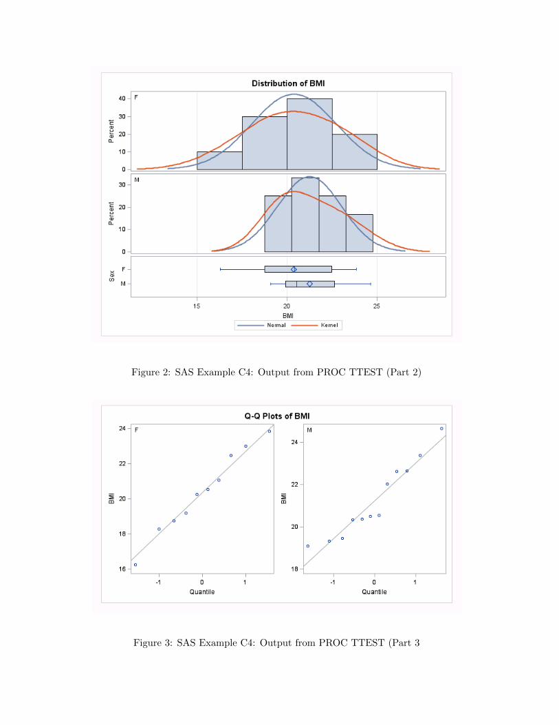
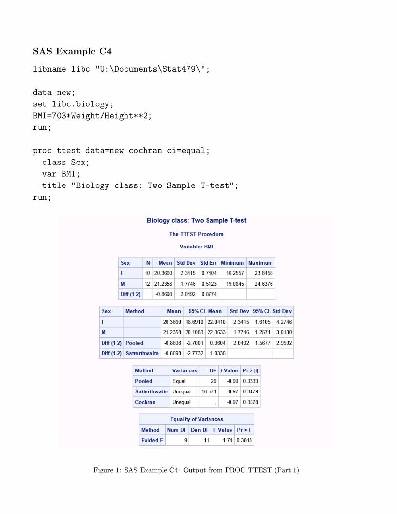
Figure 2: SAS Example C4: Output from PROC TTEST (Part 2)
Figure 3: SAS Example C4: Output from PROC TTEST (Part 3
What are SAS ODS Procedures?
• Base SAS now includes several procedures for creating plots requiredfor statistical analysis
• These create single-cell or multi-cell plots or panels of plots usingsimple syntax
• Several of these procedures will be illustrated in this section viaexamples
• A subset of the statements and options required for each procedureare presented
• The three main procs are SGPLOT, SGPANEL, and SGSCATTER
PROC SGPLOT < option(s)> ;
DENSITY response-variable </option(s)>;
DOT category-variable </option(s)>;
ELLIPSE X= numeric-variable Y= numeric-variable </option(s)>;
HBAR category-variable < /option(s) >
HBOX response-variable </option(s)>;
HISTOGRAM response-variable < /option(s)>
HLINE category-variable < /option(s)>
INSET "text-string-1" <... "text-string-n"> | (label-list);
KEYLEGEND <"name-1" ... "name-n"> </option(s)>;
LOESS X= numeric-variable Y= numeric-variable </option(s)>;
REFLINE value(s) </option(s)>;
REG X= numeric-variable Y= numeric-variable </option(s)>;
SCATTER X= variable Y= variable </option(s)>;
SERIES X= variable Y= variable </option(s)>;
STEP X= variable Y= variable </option(s)>;
VBAR category-variable < /option(s)>
VBOX response-variable </option(s)>;
VLINE category-variable < /option(s)>
XAXIS <option(s)>;
YAXIS <option(s)>;
The SGPLOT Procedure
• A few statements available in proc sgplot are illustrated via exam-ples
• The first statement discussed is the scatter statement
• The user specifies an X variable and a Y variable to be plotted onthe horizontal and the vertical axes, respectively
• This statement produces scatter plots, ordered pairs (x, y) plottedas points
• A scatter plot visually displays the relationship between the twovariables by such as trends in the data or the occurence of clustersof points
• Other than simple interpretations such as whether the relationship islinear or not, scatter plots can be used for examining more complexstatistical properties
• They can be used check whether the spread of the data values of aresponse variable change as the X values change indicating increasingvariance
Some SCATTER Statement Options
datalabel uses the Y values to label the points.
datalabel= uses the values of a variable to label the points.
group= specifies a variable that is used to group the data.
name= specifies a name for the plot.
markerattrs= specifies appearance of markers in the plot (as a style-element orusing suboptions color=,size=,symbol=.
markerchar= specifies a variable whose values replace the marker symbols inthe plot.
markercharattrs= specifies the appearance of markers in the plot when themarkerchar= option is used
Some ELLIPSE Statement Options
alpha= specifies specifies the confidence level for the ellipse.
clip the ellipse will be clipped because the axes are determined without the ellipse.
legendlabel=“text-string” specifies a label that identifies the ellipse in thelegend.
lineattrs= specifies appearance of plotted lines (as a style-element or using sub-options color=,pattern=,thickness=.
name= specifies a name for the plot.
outline|nooutline specifies whether the outlines for the bars are displayed.
type= mean | predicted specifies the type of ellipse. mean specifies a confi-dence ellipse for the population mean. predicted specifies a prediction ellipsefor a new observation. Default is predicted.
The Ellipse statement
• The ellipse statement may be used along with the scatter statementto create bivariate confidence or prediction regions for a specifiedlevel 100(1− α)%.
• These are calculated under the assumption that pairs of data values(x, y) have a bivariate normal distribution.
• A 95% prediction ellipse is generated by default. This implies thatthe probability of a point falling within the region is 0.95.
• On the other hand, one would have 95% confidence that the bivariatemean of the distribution lies within a 95% confidence ellipse.
• It is possible to draw multiple ellipses by including more than oneellipse statement specifying different types or alpha levels.
• Default legends for each ellipse, such as “95% Prediction Ellipse”are automatically generated
• The user may specify a legend label using the legendlabel= option.
• The line attributes for the outline of the region may be specifiedusing a style-element or by using suboptions

Table 1: List of Marker Symbols
Unit Description
cm centimetersin inchesmm millimeterspct or % percentagept point size, calculated at 100 dpipx pixels
Table 2: Units of Measurement
Table 3: Line Patterns
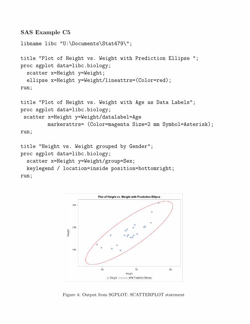
SAS Example C5
libname libc "U:\Documents\Stat479\";
title "Plot of Height vs. Weight with Prediction Ellipse ";
proc sgplot data=libc.biology;
scatter x=Height y=Weight;
ellipse x=Height y=Weight/lineattrs=(Color=red);
run;
title "Plot of Height vs. Weight with Age as Data Labels";
proc sgplot data=libc.biology;
scatter x=Height y=Weight/datalabel=Age
markerattrs= (Color=magenta Size=2 mm Symbol=Asterisk);
run;
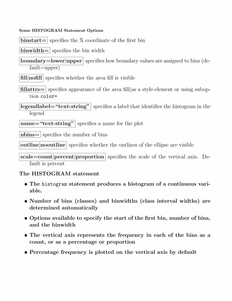
title "Height vs. Weight grouped by Gender";
proc sgplot data=libc.biology;
scatter x=Height y=Weight/group=Sex;
keylegend / location=inside position=bottomright;
run;
Figure 4: Output from SGPLOT: SCATTERPLOT statement
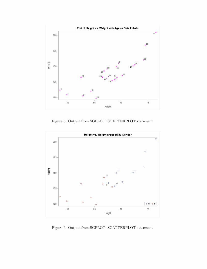
Figure 5: Output from SGPLOT: SCATTERPLOT statement
Figure 6: Output from SGPLOT: SCATTERPLOT statement
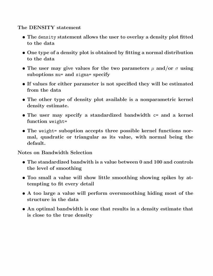
Some HISTOGRAM Statement Options
binstart= specifies the X coordinate of the first bin
binwidth= specifies the bin width
boundary=lower|upper specifies how boundary values are assigned to bins (de-fault=upper)
fill|nofill specifies whether the area fill is visible
fillattrs= specifies appearance of the area fill(as a style-element or using subop-tion color=
legendlabel=“text-string” specifies a label that identifies the histogram in thelegend
name=“text-string” specifies a name for the plot
nbins= specifies the number of bins
outline|nooutline specifies whether the outlines of the ellipse are visible
scale=count|percent|proportion specifies the scale of the vertical axis. De-fault is percent
The HISTOGRAM statement
• The histogram statement produces a histogram of a continuous vari-able.
• Number of bins (classes) and binwidths (class interval widths) aredetermined automatically
• Options available to specify the start of the first bin, number of bins,and the binwidth
• The vertical axis represents the frequency in each of the bins as acount, or as a percentage or proportion
• Percentage frequency is plotted on the vertical axis by default
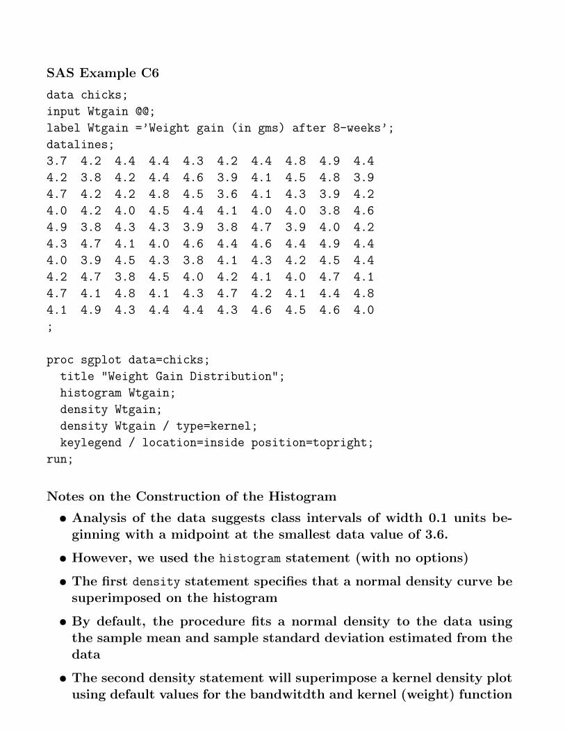
The DENSITY statement
• The density statement allows the user to overlay a density plot fittedto the data
• One type of a density plot is obtained by fitting a normal distributionto the data
• The user may give values for the two parameters µ and/or σ usingsuboptions mu= and sigma= specify
• If values for either parameter is not specified they will be estimatedfrom the data
• The other type of density plot available is a nonparametric kerneldensity estimate.
• The user may specify a standardized bandwidth c= and a kernelfunction weight=
• The weight= suboption accepts three possible kernel functions nor-mal, quadratic or triangular as its value, with normal being thedefault.
Notes on Bandwidth Selection
• The standardized bandwith is a value between 0 and 100 and controlsthe level of smoothing
• Too small a value will show little smoothing showing spikes by at-tempting to fit every detail
• A too large a value will perform oversmoothing hiding most of thestructure in the data
• An optimal bandwidth is one that results in a density estimate thatis close to the true density
SAS Example C6
data chicks;
input Wtgain @@;
label Wtgain =’Weight gain (in gms) after 8-weeks’;
datalines;
3.7 4.2 4.4 4.4 4.3 4.2 4.4 4.8 4.9 4.4
4.2 3.8 4.2 4.4 4.6 3.9 4.1 4.5 4.8 3.9
4.7 4.2 4.2 4.8 4.5 3.6 4.1 4.3 3.9 4.2
4.0 4.2 4.0 4.5 4.4 4.1 4.0 4.0 3.8 4.6
4.9 3.8 4.3 4.3 3.9 3.8 4.7 3.9 4.0 4.2
4.3 4.7 4.1 4.0 4.6 4.4 4.6 4.4 4.9 4.4
4.0 3.9 4.5 4.3 3.8 4.1 4.3 4.2 4.5 4.4
4.2 4.7 3.8 4.5 4.0 4.2 4.1 4.0 4.7 4.1
4.7 4.1 4.8 4.1 4.3 4.7 4.2 4.1 4.4 4.8
4.1 4.9 4.3 4.4 4.4 4.3 4.6 4.5 4.6 4.0
;
proc sgplot data=chicks;
title "Weight Gain Distribution";
histogram Wtgain;
density Wtgain;
density Wtgain / type=kernel;
keylegend / location=inside position=topright;
run;
Notes on the Construction of the Histogram
• Analysis of the data suggests class intervals of width 0.1 units be-ginning with a midpoint at the smallest data value of 3.6.
• However, we used the histogram statement (with no options)
• The first density statement specifies that a normal density curve besuperimposed on the histogram
• By default, the procedure fits a normal density to the data usingthe sample mean and sample standard deviation estimated from thedata
• The second density statement will superimpose a kernel density plotusing default values for the bandwitdth and kernel (weight) function
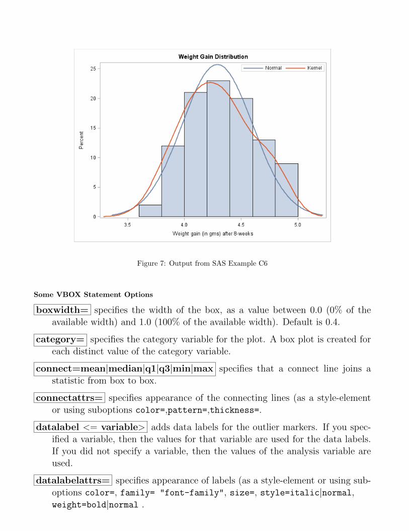
Figure 7: Output from SAS Example C6
Some VBOX Statement Options
boxwidth= specifies the width of the box, as a value between 0.0 (0% of theavailable width) and 1.0 (100% of the available width). Default is 0.4.
category= specifies the category variable for the plot. A box plot is created foreach distinct value of the category variable.
connect=mean|median|q1|q3|min|max specifies that a connect line joins astatistic from box to box.
connectattrs= specifies appearance of the connecting lines (as a style-elementor using suboptions color=,pattern=,thickness=.
datalabel <= variable> adds data labels for the outlier markers. If you spec-ified a variable, then the values for that variable are used for the data labels.If you did not specify a variable, then the values of the analysis variable areused.
datalabelattrs= specifies appearance of labels (as a style-element or using sub-options color=, family= "font-family", size=, style=italic|normal,weight=bold|normal .
fill|nofill specifies whether the boxes are filled with color.
fillattrs= specifies appearance of the fill of the boxes (as a style-element or usingsuboption color=.
group= specifies a variable that is used to group the data.
legendlabel=“text-string” specifies a label that identifies the ellipse in thelegend.
lineattrs= specifies appearance of the box outlines (as a style-element or usingsuboptions color=,pattern=,thickness=.
meanattrs= specifies appearance of the box outlines (as a style-element or usingsuboptions color=,pattern=,thickness=.
medianattrs= specifies appearance of the box outlines (as a style-element orusing suboptions color=,pattern=,thickness=.
outlierattrs= specifies appearance of the box outlines (as a style-element orusing suboptions color=,pattern=,thickness=.
percentile=1|2|3|4|5 specifies a method for computing the percentiles for theplot.
whiskerattrs= specifies appearance of the box outlines (as a style-element orusing suboptions color=,pattern=,thickness=.
name= specifies a name for the plot.
outline|nooutline specifies whether the outlines for the bars are displayed.
type= mean | predicted specifies the type of ellipse. mean specifies a confi-dence ellipse for the population mean. predicted specifies a prediction ellipsefor a new observation. Default is predicted.
SAS Example C7
data emissions;
input period @;
hc=1;
do until (hc<0);
input hc @;
if (hc<0) then return;
output;
end;
label period = ’Year of Manufacture’
hc = ’Hydrocarbon Emissions (ppm)’;
datalines;
1 2351 1293 541 1058 411 570 800 630 905 347 -1
2 620 940 350 700 1150 2000 823 1058 423 270 900 405 780 -1
3 1088 388 111 558 294 211 460 470 353 71 241 2999 199 188 353 117 -1
4 141 359 247 940 882 494 306 200 100 300 190 140 880 200 223 188 435 940 241 223 -1
5 140 160 20 20 223 60 20 95 360 70 220 400 217 58 235 1880 200 175 85 -1
;
proc format;
value pp 1=’Pre-1963’
2=’1963-1967’
3=’1968-1969’
4=’1970-1971’
5=’1972-1974’;
run;
proc sgplot data=emissions;
title "Hydrocarbon Emissions Distribution by Period";
vbox hc / category=period datalabel;
format period pp.;
run;
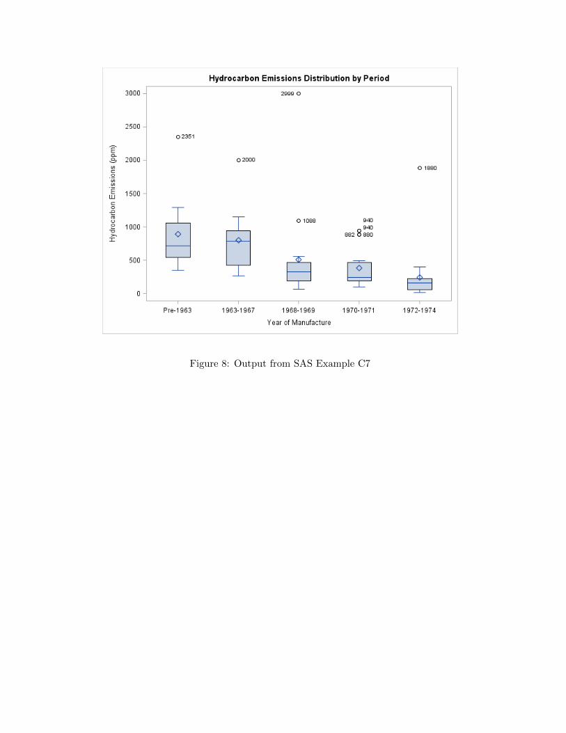
Figure 8: Output from SAS Example C7
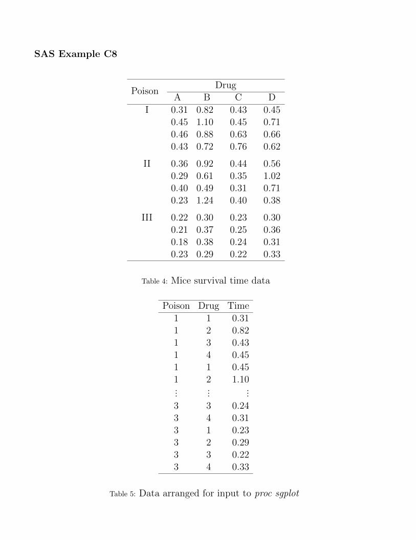
SAS Example C8
DrugPoison
A B C D
I 0.31 0.82 0.43 0.450.45 1.10 0.45 0.710.46 0.88 0.63 0.660.43 0.72 0.76 0.62
II 0.36 0.92 0.44 0.560.29 0.61 0.35 1.020.40 0.49 0.31 0.710.23 1.24 0.40 0.38
III 0.22 0.30 0.23 0.300.21 0.37 0.25 0.360.18 0.38 0.24 0.310.23 0.29 0.22 0.33
Table 4: Mice survival time data
Poison Drug Time
1 1 0.311 2 0.821 3 0.431 4 0.451 1 0.451 2 1.10...
......
3 3 0.243 4 0.313 1 0.233 2 0.293 3 0.223 4 0.33
Table 5: Data arranged for input to proc sgplot
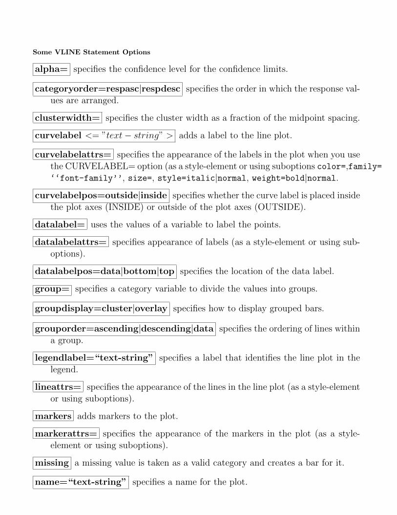
Some VLINE Statement Options
alpha= specifies the confidence level for the confidence limits.
categoryorder=respasc|respdesc specifies the order in which the response val-ues are arranged.
clusterwidth= specifies the cluster width as a fraction of the midpoint spacing.
curvelabel <= ”text− string” > adds a label to the line plot.
curvelabelattrs= specifies the appearance of the labels in the plot when you usethe CURVELABEL= option (as a style-element or using suboptions color=,family=‘‘font-family’’, size=, style=italic|normal, weight=bold|normal.
curvelabelpos=outside|inside specifies whether the curve label is placed insidethe plot axes (INSIDE) or outside of the plot axes (OUTSIDE).
datalabel= uses the values of a variable to label the points.
datalabelattrs= specifies appearance of labels (as a style-element or using sub-options).
datalabelpos=data|bottom|top specifies the location of the data label.
group= specifies a category variable to divide the values into groups.
groupdisplay=cluster|overlay specifies how to display grouped bars.
grouporder=ascending|descending|data specifies the ordering of lines withina group.
legendlabel=“text-string” specifies a label that identifies the line plot in thelegend.
lineattrs= specifies the appearance of the lines in the line plot (as a style-elementor using suboptions).
markers adds markers to the plot.
markerattrs= specifies the appearance of the markers in the plot (as a style-element or using suboptions).
missing a missing value is taken as a valid category and creates a bar for it.
name=“text-string” specifies a name for the plot.
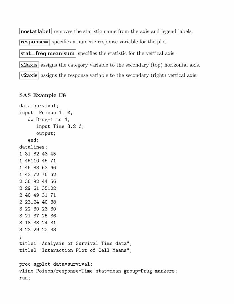
nostatlabel removes the statistic name from the axis and legend labels.
response= specifies a numeric response variable for the plot.
stat=freq|mean|sum specifies the statistic for the vertical axis.
x2axis assigns the category variable to the secondary (top) horizontal axis.
y2axis assigns the response variable to the secondary (right) vertical axis.
SAS Example C8
data survival;
input Poison 1. @;
do Drug=1 to 4;
input Time 3.2 @;
output;
end;
datalines;
1 31 82 43 45
1 45110 45 71
1 46 88 63 66
1 43 72 76 62
2 36 92 44 56
2 29 61 35102
2 40 49 31 71
2 23124 40 38
3 22 30 23 30
3 21 37 25 36
3 18 38 24 31
3 23 29 22 33
;
title1 "Analysis of Survival Time data";
title2 "Interaction Plot of Cell Means";
proc sgplot data=survival;
vline Poison/response=Time stat=mean group=Drug markers;
run;
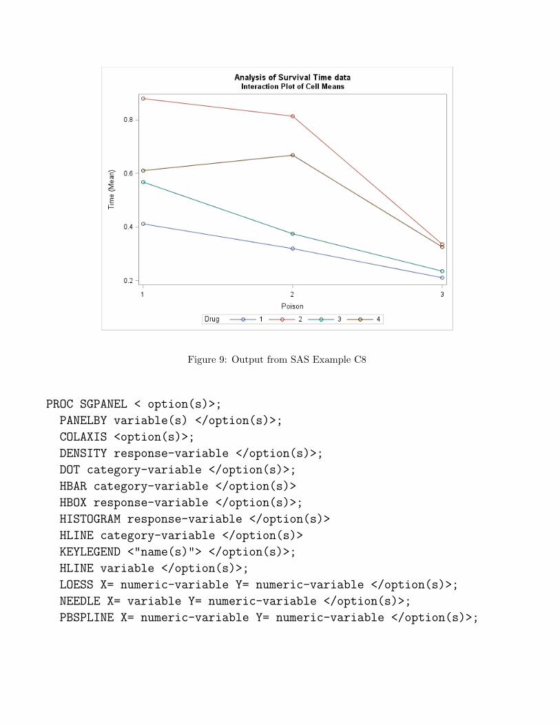
Figure 9: Output from SAS Example C8
PROC SGPANEL < option(s)>;
PANELBY variable(s) </option(s)>;
COLAXIS <option(s)>;
DENSITY response-variable </option(s)>;
DOT category-variable </option(s)>;
HBAR category-variable </option(s)>
HBOX response-variable </option(s)>;
HISTOGRAM response-variable </option(s)>
HLINE category-variable </option(s)>
KEYLEGEND <"name(s)"> </option(s)>;
HLINE variable </option(s)>;
LOESS X= numeric-variable Y= numeric-variable </option(s)>;
NEEDLE X= variable Y= numeric-variable </option(s)>;
PBSPLINE X= numeric-variable Y= numeric-variable </option(s)>;
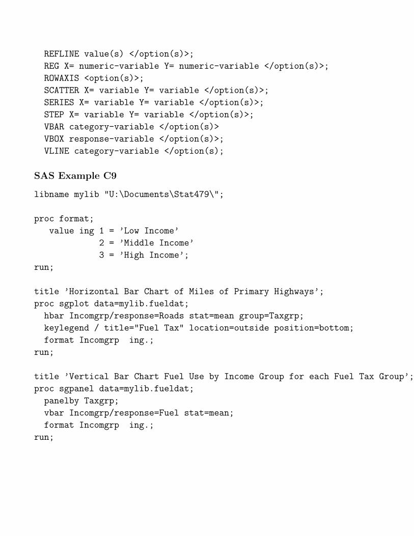
REFLINE value(s) </option(s)>;
REG X= numeric-variable Y= numeric-variable </option(s)>;
ROWAXIS <option(s)>;
SCATTER X= variable Y= variable </option(s)>;
SERIES X= variable Y= variable </option(s)>;
STEP X= variable Y= variable </option(s)>;
VBAR category-variable </option(s)>
VBOX response-variable </option(s)>;
VLINE category-variable </option(s);
SAS Example C9
libname mylib "U:\Documents\Stat479\";
proc format;
value ing 1 = ’Low Income’
2 = ’Middle Income’
3 = ’High Income’;
run;
title ’Horizontal Bar Chart of Miles of Primary Highways’;
proc sgplot data=mylib.fueldat;
hbar Incomgrp/response=Roads stat=mean group=Taxgrp;
keylegend / title="Fuel Tax" location=outside position=bottom;
format Incomgrp ing.;
run;
title ’Vertical Bar Chart Fuel Use by Income Group for each Fuel Tax Group’;
proc sgpanel data=mylib.fueldat;
panelby Taxgrp;
vbar Incomgrp/response=Fuel stat=mean;
format Incomgrp ing.;
run;
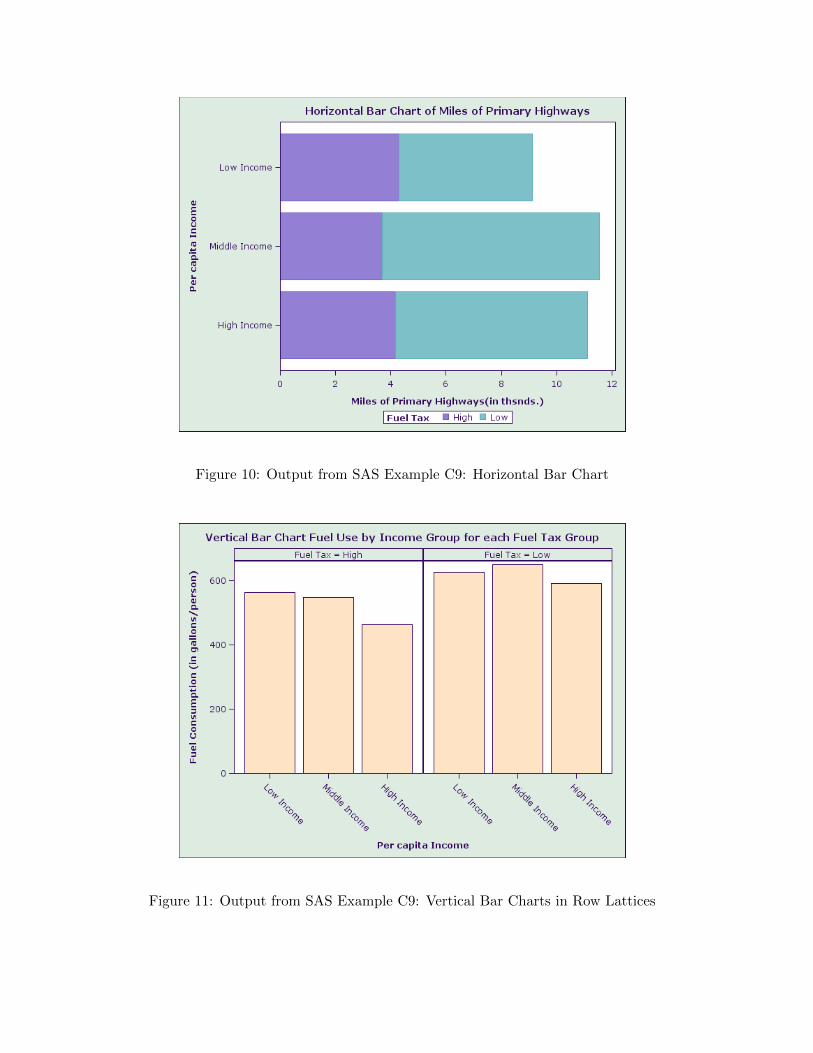
Figure 10: Output from SAS Example C9: Horizontal Bar Chart
Figure 11: Output from SAS Example C9: Vertical Bar Charts in Row Lattices
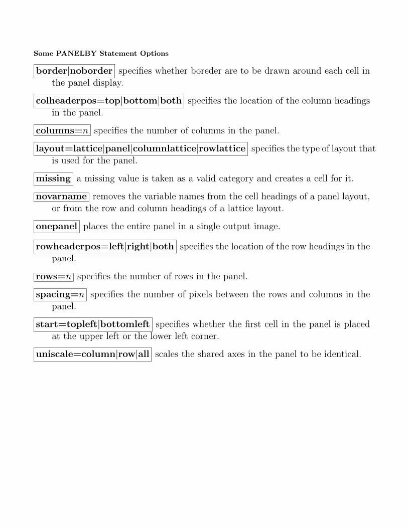
Some PANELBY Statement Options
border|noborder specifies whether boreder are to be drawn around each cell inthe panel display.
colheaderpos=top|bottom|both specifies the location of the column headingsin the panel.
columns=n specifies the number of columns in the panel.
layout=lattice|panel|columnlattice|rowlattice specifies the type of layout thatis used for the panel.
missing a missing value is taken as a valid category and creates a cell for it.
novarname removes the variable names from the cell headings of a panel layout,or from the row and column headings of a lattice layout.
onepanel places the entire panel in a single output image.
rowheaderpos=left|right|both specifies the location of the row headings in thepanel.
rows=n specifies the number of rows in the panel.
spacing=n specifies the number of pixels between the rows and columns in thepanel.
start=topleft|bottomleft specifies whether the first cell in the panel is placedat the upper left or the lower left corner.
uniscale=column|row|all scales the shared axes in the panel to be identical.
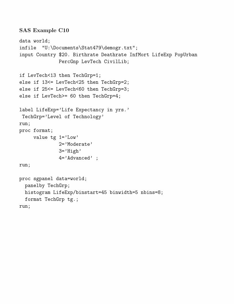
SAS Example C10
data world;
infile "U:\Documents\Stat479\demogr.txt";
input Country $20. Birthrate Deathrate InfMort LifeExp PopUrban
PercGnp LevTech CivilLib;
if LevTech<13 then TechGrp=1;
else if 13<= LevTech<25 then TechGrp=2;
else if 25<= LevTech<60 then TechGrp=3;
else if LevTech>= 60 then TechGrp=4;
label LifeExp=’Life Expectancy in yrs.’
TechGrp=’Level of Technology’
run;
proc format;
value tg 1=’Low’
2=’Moderate’
3=’High’
4=’Advanced’ ;
run;
proc sgpanel data=world;
panelby TechGrp;
histogram LifeExp/binstart=45 binwidth=5 nbins=8;
format TechGrp tg.;
run;
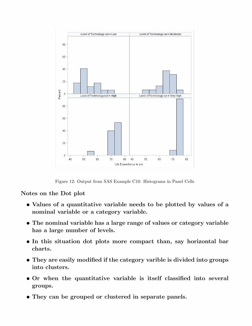
Figure 12: Output from SAS Example C10: Histograms in Panel Cells
Notes on the Dot plot
• Values of a quantitative variable needs to be plotted by values of anominal variable or a category variable.
• The nominal variable has a large range of values or category variablehas a large number of levels.
• In this situation dot plots more compact than, say horizontal barcharts.
• They are easily modified if the category varible is divided into groupsinto clusters.
• Or when the quantitative variable is itself classified into severalgroups.
• They can be grouped or clustered in separate panels.
SAS Example C11
libname mylib "U:\Documents\Stat479\";
proc sgpanel data=mylib.fueldat;
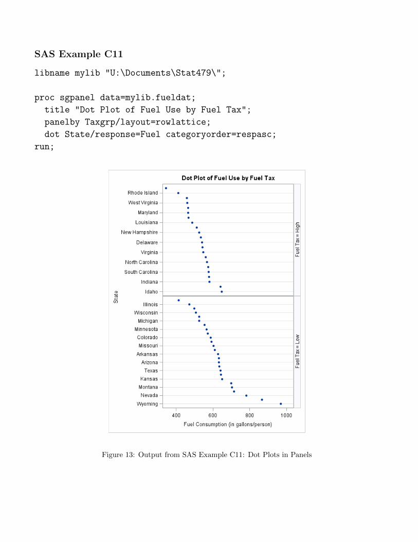
title "Dot Plot of Fuel Use by Fuel Tax";
panelby Taxgrp/layout=rowlattice;
dot State/response=Fuel categoryorder=respasc;
run;
Figure 13: Output from SAS Example C11: Dot Plots in Panels
SAS Example C12
data world;
infile "U:\Documents\Stat479\demogr.txt";
input Country $20. Birthrate Deathrate InfMort LifeExp PopUrban
PercGnp LevTech CivilLib;
label Birthrate=’Crude Birth Rate’
Deathrate=’Crude Death Rate’
InfMort=’Infant Mortality Rate’
LifeExp=’Life Expectancy in yrs.’
PopUrban=’Percent of Urban Population’
PercGnp=’Per capita GNP in U.S. dollars’
LevTech=’Level of Technology’
CivilLib=’Degree of Denial of Civil Liberties’;
if LevTech<13 then TechGrp=1;
else if 13<= LevTech<25 then TechGrp=2;
else if 25<= LevTech<60 then TechGrp=3;
else if LevTech>= 60 then TechGrp=4;
label TechGrp=’Level of Technology’;
run;
proc format;
value tg 1=’Low’
2=’Moderate’
3=’High’
4=’Very High’ ;
run;
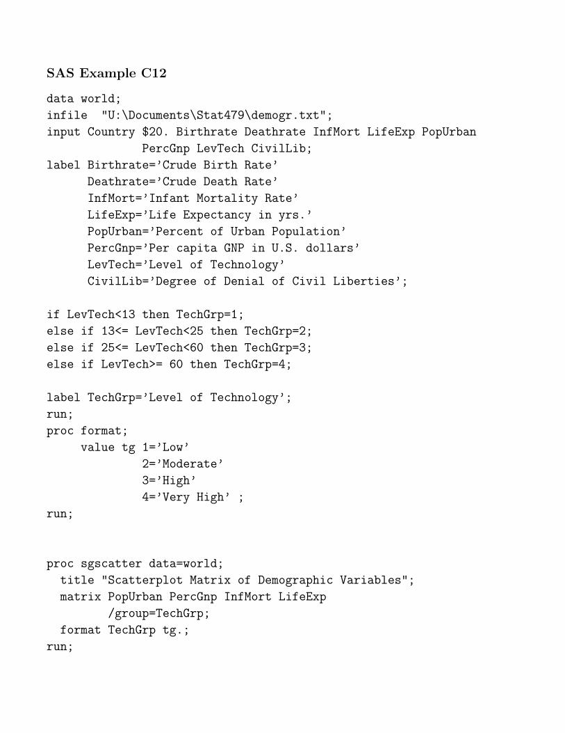
proc sgscatter data=world;
title "Scatterplot Matrix of Demographic Variables";
matrix PopUrban PercGnp InfMort LifeExp
/group=TechGrp;
format TechGrp tg.;
run;

Figure 14: Output from SAS Example C12: Scatter Plot Matrix of world demographic data