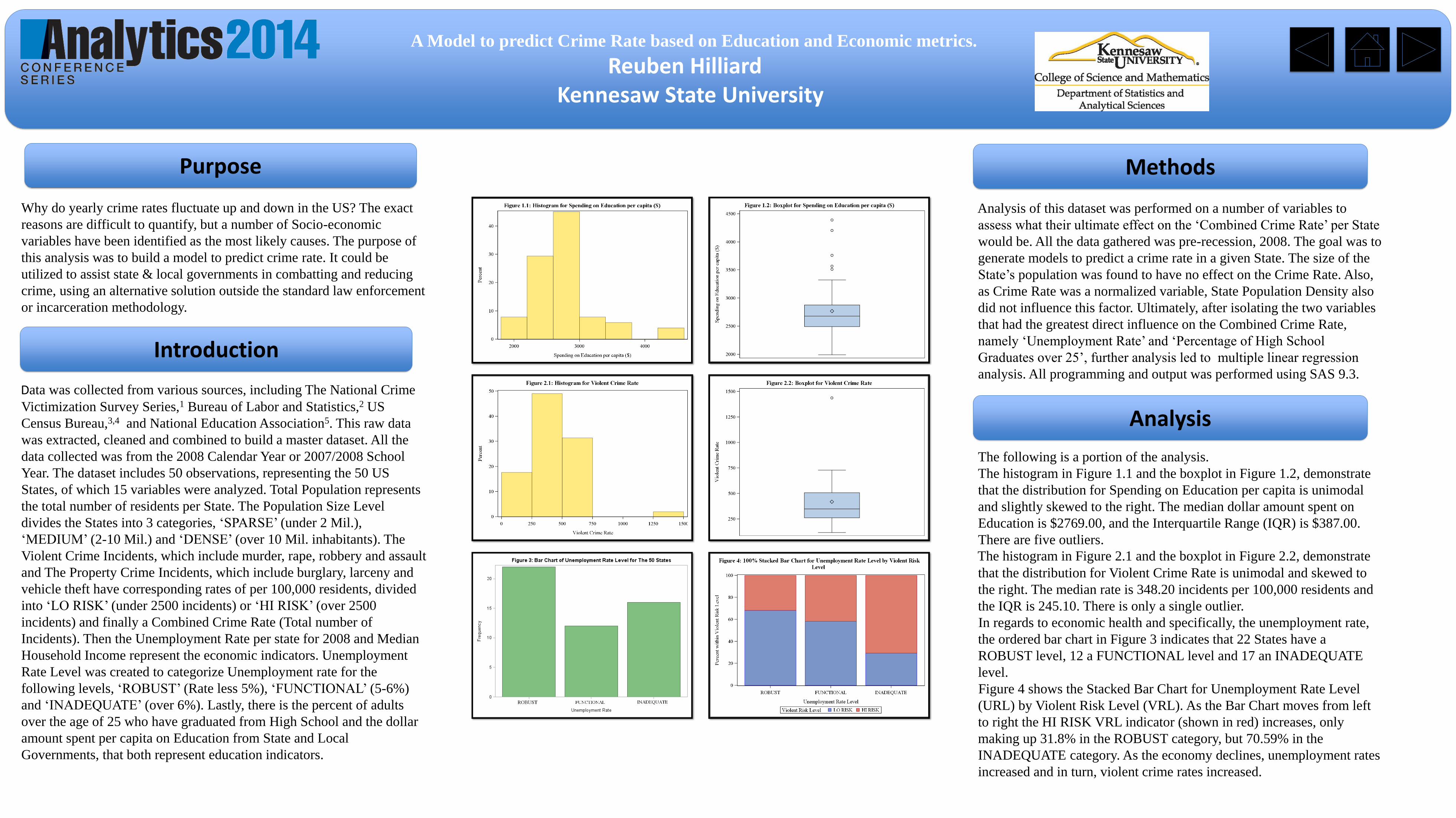
A Model to predict Crime Rate based on Education and Economic metrics.

Reuben HilliardKennesaw State University

Purpose Methods

Why do yearly crime rates fluctuate up and down in the US? The exact

reasons are difficult to quantify, but a number of Socio-economic

variables have been identified as the most likely causes. The purpose of

this analysis was to build a model to predict crime rate. It could be

utilized to assist state & local governments in combatting and reducing

crime, using an alternative solution outside the standard law enforcement

or incarceration methodology.

Data was collected from various sources, including The National Crime

Victimization Survey Series,1 Bureau of Labor and Statistics,2 US

Census Bureau,3,4 and National Education Association5. This raw data

was extracted, cleaned and combined to build a master dataset. All the

data collected was from the 2008 Calendar Year or 2007/2008 School

Year. The dataset includes 50 observations, representing the 50 US

States, of which 15 variables were analyzed. Total Population represents

the total number of residents per State. The Population Size Level

divides the States into 3 categories, ‘SPARSE’ (under 2 Mil.),

‘MEDIUM’ (2-10 Mil.) and ‘DENSE’ (over 10 Mil. inhabitants). The

Violent Crime Incidents, which include murder, rape, robbery and assault

and The Property Crime Incidents, which include burglary, larceny and

vehicle theft have corresponding rates of per 100,000 residents, divided

into ‘LO RISK’ (under 2500 incidents) or ‘HI RISK’ (over 2500

incidents) and finally a Combined Crime Rate (Total number of

Incidents). Then the Unemployment Rate per state for 2008 and Median

Household Income represent the economic indicators. Unemployment

Rate Level was created to categorize Unemployment rate for the

following levels, ‘ROBUST’ (Rate less 5%), ‘FUNCTIONAL’ (5-6%)

and ‘INADEQUATE’ (over 6%). Lastly, there is the percent of adults

over the age of 25 who have graduated from High School and the dollar

amount spent per capita on Education from State and Local

Governments, that both represent education indicators.

Analysis of this dataset was performed on a number of variables to

assess what their ultimate effect on the ‘Combined Crime Rate’ per State

would be. All the data gathered was pre-recession, 2008. The goal was to

generate models to predict a crime rate in a given State. The size of the

State’s population was found to have no effect on the Crime Rate. Also,

as Crime Rate was a normalized variable, State Population Density also

did not influence this factor. Ultimately, after isolating the two variables

that had the greatest direct influence on the Combined Crime Rate,

namely ‘Unemployment Rate’ and ‘Percentage of High School

Graduates over 25’, further analysis led to multiple linear regression

analysis. All programming and output was performed using SAS 9.3.

The following is a portion of the analysis.

The histogram in Figure 1.1 and the boxplot in Figure 1.2, demonstrate

that the distribution for Spending on Education per capita is unimodal

and slightly skewed to the right. The median dollar amount spent on

Education is $2769.00, and the Interquartile Range (IQR) is $387.00.

There are five outliers.

The histogram in Figure 2.1 and the boxplot in Figure 2.2, demonstrate

that the distribution for Violent Crime Rate is unimodal and skewed to

the right. The median rate is 348.20 incidents per 100,000 residents and

the IQR is 245.10. There is only a single outlier.

In regards to economic health and specifically, the unemployment rate,

the ordered bar chart in Figure 3 indicates that 22 States have a

ROBUST level, 12 a FUNCTIONAL level and 17 an INADEQUATE

level.

Figure 4 shows the Stacked Bar Chart for Unemployment Rate Level

(URL) by Violent Risk Level (VRL). As the Bar Chart moves from left

to right the HI RISK VRL indicator (shown in red) increases, only

making up 31.8% in the ROBUST category, but 70.59% in the

INADEQUATE category. As the economy declines, unemployment rates

increased and in turn, violent crime rates increased.

Introduction

Analysis

A Model to predict Crime Rate based on Education and Economic metrics.

Reuben HilliardKennesaw State University

Conclusion

References

1. The National Crime Victimization Survey, 2008. Web retrieved 4/12/2014.

https://explore.data.gov/Law-Enforcement-Courts-and-Prisons/National-

Crime-Victimization-Survey-2008-Record-Ty/rfme-ynch

2. Unemployment Rate, 2008. Web retrieved 4/12/2014.

http://www.bls.gov/lau/lastrk08.htm

3. Median Family Income, Wage Census 2008. Web retrieved 4/12/2014.

http://www.census.gov/hhes/www/income/data/statemedian/

4. State Education Levels, 2008. Web retrieved 4/12/2014.

http://www.census.gov/compendia/statab/2011/tables/11s0229.pdf

5. Per Capita Spending on Education, 2007/2008. Web retrieved 4/12/2014.

http://www.nea.org/assets/docs/HE/NEA_Rankings_and_Estimates010711.pdf

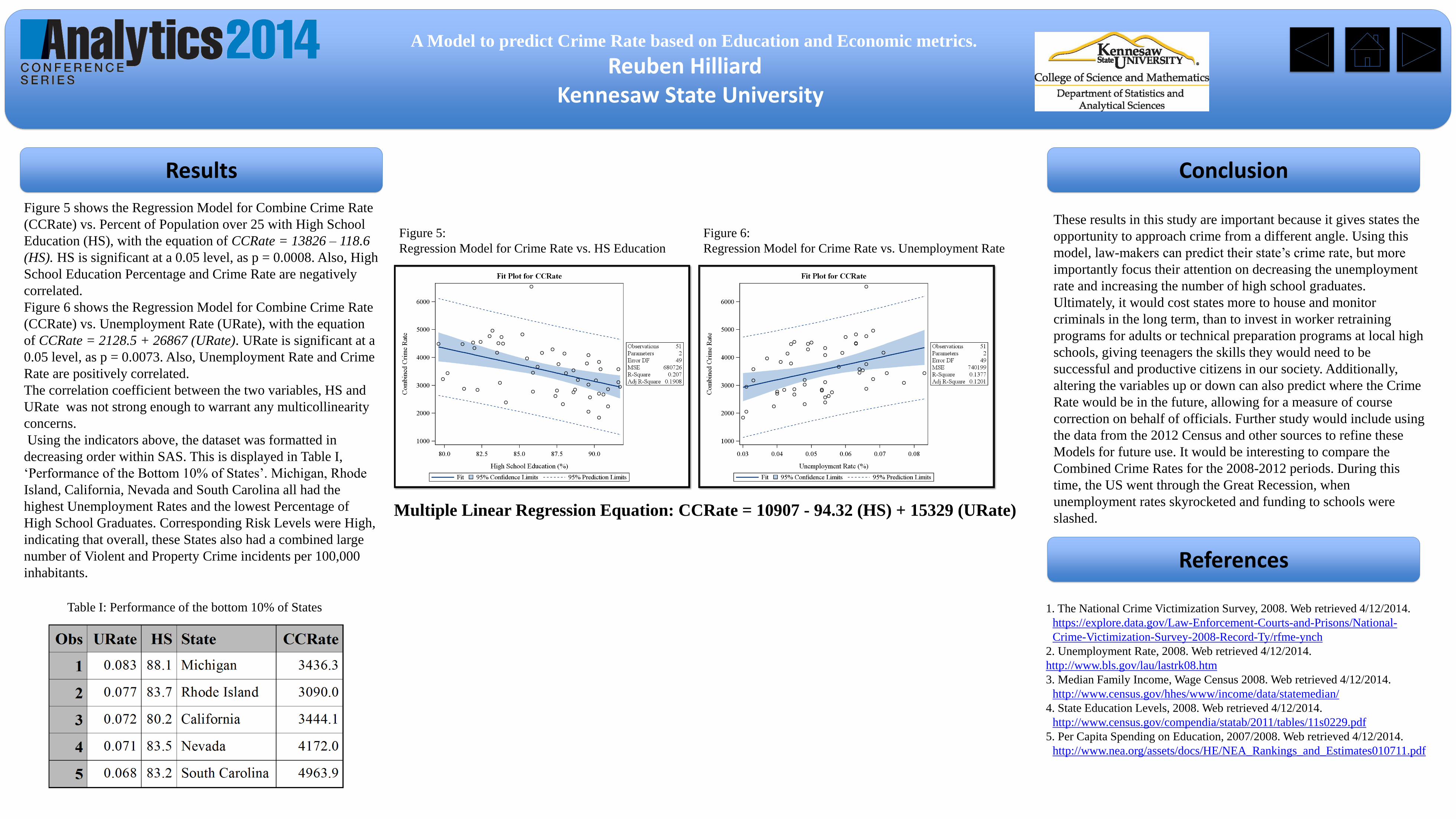
These results in this study are important because it gives states the

opportunity to approach crime from a different angle. Using this

model, law-makers can predict their state’s crime rate, but more

importantly focus their attention on decreasing the unemployment

rate and increasing the number of high school graduates.

Ultimately, it would cost states more to house and monitor

criminals in the long term, than to invest in worker retraining

programs for adults or technical preparation programs at local high

schools, giving teenagers the skills they would need to be

successful and productive citizens in our society. Additionally,

altering the variables up or down can also predict where the Crime

Rate would be in the future, allowing for a measure of course

correction on behalf of officials. Further study would include using

the data from the 2012 Census and other sources to refine these

Models for future use. It would be interesting to compare the

Combined Crime Rates for the 2008-2012 periods. During this

time, the US went through the Great Recession, when

unemployment rates skyrocketed and funding to schools were

slashed. Multiple Linear Regression Equation: CCRate = 10907 - 94.32 (HS) + 15329 (URate)

Figure 5:

Regression Model for Crime Rate vs. HS Education

Figure 6:

Regression Model for Crime Rate vs. Unemployment Rate

Table I: Performance of the bottom 10% of States

Results

Figure 5 shows the Regression Model for Combine Crime Rate

(CCRate) vs. Percent of Population over 25 with High School

Education (HS), with the equation of CCRate = 13826 – 118.6

(HS). HS is significant at a 0.05 level, as p = 0.0008. Also, High

School Education Percentage and Crime Rate are negatively

correlated.

Figure 6 shows the Regression Model for Combine Crime Rate

(CCRate) vs. Unemployment Rate (URate), with the equation

of CCRate = 2128.5 + 26867 (URate). URate is significant at a

0.05 level, as p = 0.0073. Also, Unemployment Rate and Crime

Rate are positively correlated.

The correlation coefficient between the two variables, HS and

URate was not strong enough to warrant any multicollinearity

concerns.

Using the indicators above, the dataset was formatted in

decreasing order within SAS. This is displayed in Table I,

‘Performance of the Bottom 10% of States’. Michigan, Rhode

Island, California, Nevada and South Carolina all had the

highest Unemployment Rates and the lowest Percentage of

High School Graduates. Corresponding Risk Levels were High,

indicating that overall, these States also had a combined large

number of Violent and Property Crime incidents per 100,000

inhabitants.

A Model to predict Crime Rate based on Education and Economic metrics.

Reuben HilliardKennesaw State University

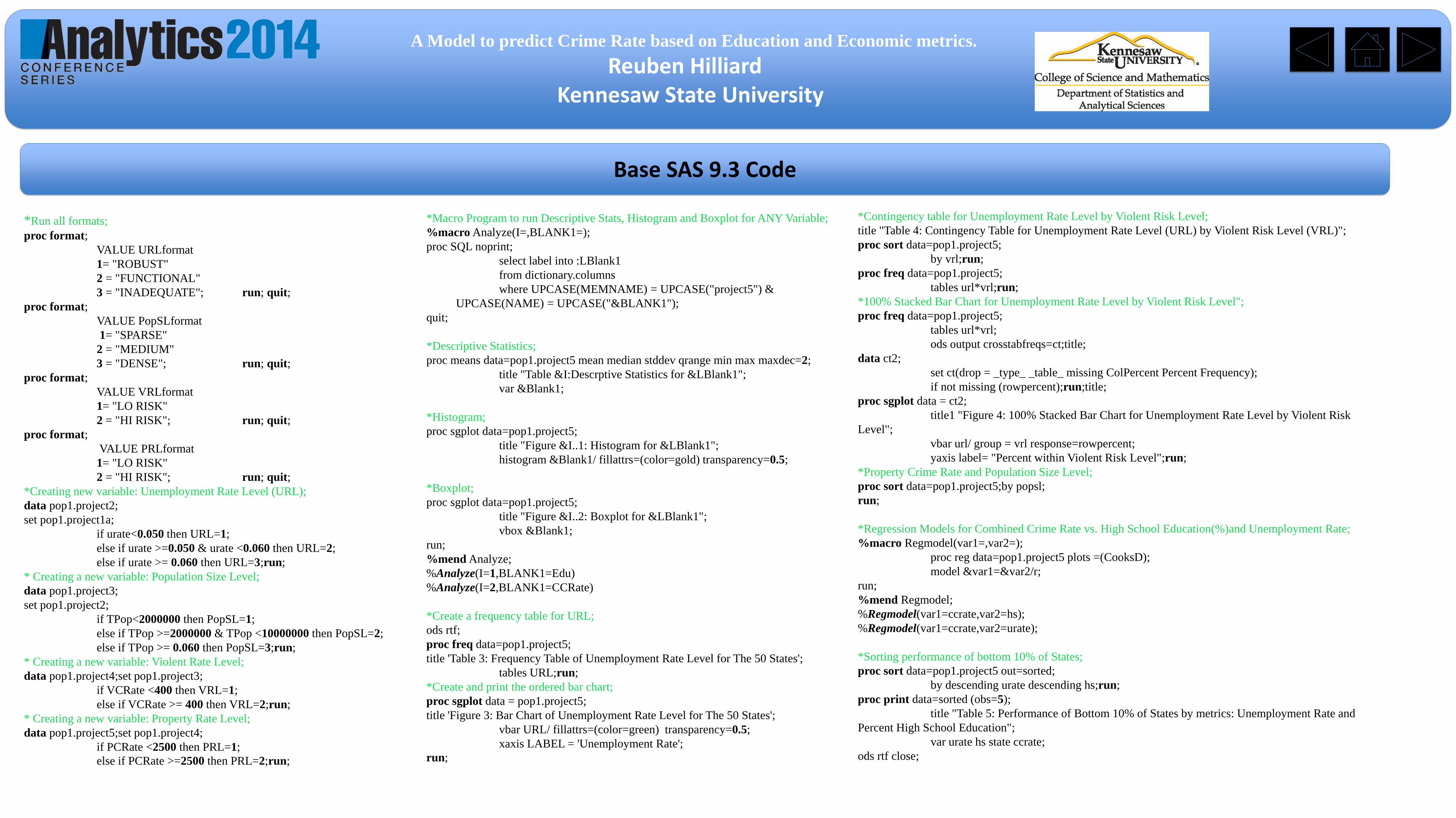
Base SAS 9.3 Code

*Contingency table for Unemployment Rate Level by Violent Risk Level;

title "Table 4: Contingency Table for Unemployment Rate Level (URL) by Violent Risk Level (VRL)";

proc sort data=pop1.project5;

by vrl;run;

proc freq data=pop1.project5;

tables url*vrl;run;

*100% Stacked Bar Chart for Unemployment Rate Level by Violent Risk Level";

proc freq data=pop1.project5;

tables url*vrl;

ods output crosstabfreqs=ct;title;

data ct2;

set ct(drop = _type_ _table_ missing ColPercent Percent Frequency);

if not missing (rowpercent);run;title;

proc sgplot data = ct2;

title1 "Figure 4: 100% Stacked Bar Chart for Unemployment Rate Level by Violent Risk

Level";

vbar url/ group = vrl response=rowpercent;

yaxis label= "Percent within Violent Risk Level";run;

*Property Crime Rate and Population Size Level;

proc sort data=pop1.project5;by popsl;

run;

*Regression Models for Combined Crime Rate vs. High School Education(%)and Unemployment Rate;

%macro Regmodel(var1=,var2=);

proc reg data=pop1.project5 plots =(CooksD);

model &var1=&var2/r;

run;

%mend Regmodel;

%Regmodel(var1=ccrate,var2=hs);

%Regmodel(var1=ccrate,var2=urate);

*Sorting performance of bottom 10% of States;

proc sort data=pop1.project5 out=sorted;

by descending urate descending hs;run;

proc print data=sorted (obs=5);

title "Table 5: Performance of Bottom 10% of States by metrics: Unemployment Rate and

Percent High School Education";

var urate hs state ccrate;

ods rtf close;

*Run all formats;

proc format;

VALUE URLformat

1= "ROBUST"

2 = "FUNCTIONAL"

3 = "INADEQUATE"; run; quit;

proc format;

VALUE PopSLformat

1= "SPARSE"

2 = "MEDIUM"

3 = "DENSE"; run; quit;

proc format;

VALUE VRLformat

1= "LO RISK"

2 = "HI RISK"; run; quit;

proc format;

VALUE PRLformat

1= "LO RISK"

2 = "HI RISK"; run; quit;

*Creating new variable: Unemployment Rate Level (URL);

data pop1.project2;

set pop1.project1a;

if urate<0.050 then URL=1;

else if urate >=0.050 & urate <0.060 then URL=2;

else if urate >= 0.060 then URL=3;run;

* Creating a new variable: Population Size Level;

data pop1.project3;

set pop1.project2;

if TPop<2000000 then PopSL=1;

else if TPop >=2000000 & TPop <10000000 then PopSL=2;

else if TPop >= 0.060 then PopSL=3;run;

* Creating a new variable: Violent Rate Level;

data pop1.project4;set pop1.project3;

if VCRate <400 then VRL=1;

else if VCRate >= 400 then VRL=2;run;

* Creating a new variable: Property Rate Level;

data pop1.project5;set pop1.project4;

if PCRate <2500 then PRL=1;

else if PCRate >=2500 then PRL=2;run;

*Macro Program to run Descriptive Stats, Histogram and Boxplot for ANY Variable;

%macro Analyze(I=,BLANK1=);

proc SQL noprint;

select label into :LBlank1

from dictionary.columns

where UPCASE(MEMNAME) = UPCASE("project5") &

UPCASE(NAME) = UPCASE("&BLANK1");

quit;

*Descriptive Statistics;

proc means data=pop1.project5 mean median stddev qrange min max maxdec=2;

title "Table &I:Descrptive Statistics for &LBlank1";

var &Blank1;

*Histogram;

proc sgplot data=pop1.project5;

title "Figure &I..1: Histogram for &LBlank1";

histogram &Blank1/ fillattrs=(color=gold) transparency=0.5;

*Boxplot;

proc sgplot data=pop1.project5;

title "Figure &I..2: Boxplot for &LBlank1";

vbox &Blank1;

run;

%mend Analyze;

%Analyze(I=1,BLANK1=Edu)

%Analyze(I=2,BLANK1=CCRate)

*Create a frequency table for URL;

ods rtf;

proc freq data=pop1.project5;

title 'Table 3: Frequency Table of Unemployment Rate Level for The 50 States';

tables URL;run;

*Create and print the ordered bar chart;

proc sgplot data = pop1.project5;

title 'Figure 3: Bar Chart of Unemployment Rate Level for The 50 States';

vbar URL/ fillattrs=(color=green) transparency=0.5;

xaxis LABEL = 'Unemployment Rate';

run;