Embed Size (px)
Citation preview
SAS® 9.3ODS Graphics EditorUser’s Guide
SAS® Documentation

The correct bibliographic citation for this manual is as follows: SAS Institute Inc. 2011. SAS® 9.3 ODS Graphics Editor: User's Guide. Cary, NC: .
SAS® 9.3: ODS Graphics Editor User's Guide
Copyright © 2011, SAS Institute Inc., Cary, NC, USA
All rights reserved. Produced in the United States of America.
For a hardcopy book: No part of this publication may be reproduced, stored in a retrieval system, or transmitted, in any form or by any means,electronic, mechanical, photocopying, or otherwise, without the prior written permission of the publisher, SAS Institute Inc.
For a Web download or e-book:Your use of this publication shall be governed by the terms established by the vendor at the time you acquire thispublication.
The scanning, uploading, and distribution of this book via the Internet or any other means without the permission of the publisher is illegal andpunishable by law. Please purchase only authorized electronic editions and do not participate in or encourage electronic piracy of copyrightedmaterials. Your support of others' rights is appreciated.
U.S. Government Restricted Rights Notice: Use, duplication, or disclosure of this software and related documentation by the U.S. government issubject to the Agreement with SAS Institute and the restrictions set forth in FAR 52.227–19 Commercial Computer Software-Restricted Rights(June 1987).
SAS Institute Inc., SAS Campus Drive, Cary, North Carolina.
1st printing, July 2011
SAS® Publishing provides a complete selection of books and electronic products to help customers use SAS software to its fullest potential. Formore information about our e-books, e-learning products, CDs, and hard-copy books, visit the SAS Publishing Web site atsupport.sas.com/publishing or call 1-800-727-3228.
SAS® and all other SAS Institute Inc. product or service names are registered trademarks or trademarks of SAS Institute Inc. in the USA and othercountries. ® indicates USA registration.
Other brand and product names are registered trademarks or trademarks of their respective companies.
Contents
What's New in the SAS 9.3 ODS Graphics Editor . . . . . . . . . . . . . . . . . . . . . . . . . . . . . vii
PART 1 Introduction to the ODS Graphics Editor 1
Chapter 1 • Overview of the ODS Graphics Editor . . . . . . . . . . . . . . . . . . . . . . . . . . . . . . . . . . . . . 3What Is the SAS ODS Graphics Editor? . . . . . . . . . . . . . . . . . . . . . . . . . . . . . . . . . . . . . 3Why Use the ODS Graphics Editor? . . . . . . . . . . . . . . . . . . . . . . . . . . . . . . . . . . . . . . . . 3Key Features of the ODS Graphics Editor . . . . . . . . . . . . . . . . . . . . . . . . . . . . . . . . . . . . 4Types of Files That Can Be Edited . . . . . . . . . . . . . . . . . . . . . . . . . . . . . . . . . . . . . . . . . . 4Components of a Graph . . . . . . . . . . . . . . . . . . . . . . . . . . . . . . . . . . . . . . . . . . . . . . . . . . 5General Editing and Annotation Concepts . . . . . . . . . . . . . . . . . . . . . . . . . . . . . . . . . . . . 6Use of Locale . . . . . . . . . . . . . . . . . . . . . . . . . . . . . . . . . . . . . . . . . . . . . . . . . . . . . . . . . . 6
Chapter 2 • Getting Started with the ODS Graphics Editor . . . . . . . . . . . . . . . . . . . . . . . . . . . . . . 7Using a Stand-Alone ODS Graphics Editor . . . . . . . . . . . . . . . . . . . . . . . . . . . . . . . . . . . 7Creating Editable Graphics . . . . . . . . . . . . . . . . . . . . . . . . . . . . . . . . . . . . . . . . . . . . . . . . 8Open an ODS Graph for Editing . . . . . . . . . . . . . . . . . . . . . . . . . . . . . . . . . . . . . . . . . . . 9About SGE Files Generated on z/OS Systems . . . . . . . . . . . . . . . . . . . . . . . . . . . . . . . . . 9About the Graph Toolbar . . . . . . . . . . . . . . . . . . . . . . . . . . . . . . . . . . . . . . . . . . . . . . . . 10Save Graph Output . . . . . . . . . . . . . . . . . . . . . . . . . . . . . . . . . . . . . . . . . . . . . . . . . . . . . 11Print Graph Output . . . . . . . . . . . . . . . . . . . . . . . . . . . . . . . . . . . . . . . . . . . . . . . . . . . . . 11Copy and Paste a Graph . . . . . . . . . . . . . . . . . . . . . . . . . . . . . . . . . . . . . . . . . . . . . . . . . 12Create a New Blank Window . . . . . . . . . . . . . . . . . . . . . . . . . . . . . . . . . . . . . . . . . . . . . 12
PART 2 Editing Graphs 13
Chapter 3 • Modifying General Graph Properties . . . . . . . . . . . . . . . . . . . . . . . . . . . . . . . . . . . . . 15Specify a Style for a Graph . . . . . . . . . . . . . . . . . . . . . . . . . . . . . . . . . . . . . . . . . . . . . . . 15Resize a Graph . . . . . . . . . . . . . . . . . . . . . . . . . . . . . . . . . . . . . . . . . . . . . . . . . . . . . . . . 16Change the Background Color of a Graph . . . . . . . . . . . . . . . . . . . . . . . . . . . . . . . . . . . 17
Chapter 4 • Working with Titles and Footnotes . . . . . . . . . . . . . . . . . . . . . . . . . . . . . . . . . . . . . . . 19About Titles and Footnotes . . . . . . . . . . . . . . . . . . . . . . . . . . . . . . . . . . . . . . . . . . . . . . . 19Add a Title or Footnote to a Graph . . . . . . . . . . . . . . . . . . . . . . . . . . . . . . . . . . . . . . . . . 19Edit or Format a Title or Footnote . . . . . . . . . . . . . . . . . . . . . . . . . . . . . . . . . . . . . . . . . 20Using the Formatting Toolbar . . . . . . . . . . . . . . . . . . . . . . . . . . . . . . . . . . . . . . . . . . . . 21Using the Color List Box . . . . . . . . . . . . . . . . . . . . . . . . . . . . . . . . . . . . . . . . . . . . . . . . 22Aligning a Title or Footnote in a Graph . . . . . . . . . . . . . . . . . . . . . . . . . . . . . . . . . . . . . 23Move a Title or Footnote in a Graph . . . . . . . . . . . . . . . . . . . . . . . . . . . . . . . . . . . . . . . 24Delete a Title or Footnote from a Graph . . . . . . . . . . . . . . . . . . . . . . . . . . . . . . . . . . . . 25Use of Alternate Short Text in Graph Elements . . . . . . . . . . . . . . . . . . . . . . . . . . . . . . . 25
Chapter 5 • Working with Legends . . . . . . . . . . . . . . . . . . . . . . . . . . . . . . . . . . . . . . . . . . . . . . . . . 27Add or Edit a Legend Title . . . . . . . . . . . . . . . . . . . . . . . . . . . . . . . . . . . . . . . . . . . . . . . 27Change the Outline and Background Color of a Legend . . . . . . . . . . . . . . . . . . . . . . . . 27
Move a Legend Inside or Outside a Plot . . . . . . . . . . . . . . . . . . . . . . . . . . . . . . . . . . . . 28
Chapter 6 • Modifying Plot and Axis Properties . . . . . . . . . . . . . . . . . . . . . . . . . . . . . . . . . . . . . . 31Working with Plot Properties . . . . . . . . . . . . . . . . . . . . . . . . . . . . . . . . . . . . . . . . . . . . . 31Working with Axis Properties . . . . . . . . . . . . . . . . . . . . . . . . . . . . . . . . . . . . . . . . . . . . 36Working with Axis Labels . . . . . . . . . . . . . . . . . . . . . . . . . . . . . . . . . . . . . . . . . . . . . . . 36Edit an Existing Axis Label . . . . . . . . . . . . . . . . . . . . . . . . . . . . . . . . . . . . . . . . . . . . . . 37Add an Axis Label . . . . . . . . . . . . . . . . . . . . . . . . . . . . . . . . . . . . . . . . . . . . . . . . . . . . . 37Show or Hide an Axis Label . . . . . . . . . . . . . . . . . . . . . . . . . . . . . . . . . . . . . . . . . . . . . . 37Delete an Axis Label . . . . . . . . . . . . . . . . . . . . . . . . . . . . . . . . . . . . . . . . . . . . . . . . . . . 38
Chapter 7 • Working with Data Labels and Multi-Cell Graphs . . . . . . . . . . . . . . . . . . . . . . . . . . . 39Display or Hide Data Labels . . . . . . . . . . . . . . . . . . . . . . . . . . . . . . . . . . . . . . . . . . . . . . 39Working with Multi-Cell Graphs . . . . . . . . . . . . . . . . . . . . . . . . . . . . . . . . . . . . . . . . . . 40
PART 3 Annotating Graphs 43
Chapter 8 • Annotation Overview . . . . . . . . . . . . . . . . . . . . . . . . . . . . . . . . . . . . . . . . . . . . . . . . . . 45About Annotation Objects . . . . . . . . . . . . . . . . . . . . . . . . . . . . . . . . . . . . . . . . . . . . . . . 45Understanding Annotation Objects and Data . . . . . . . . . . . . . . . . . . . . . . . . . . . . . . . . . 45Data Attachment Examples for Annotations . . . . . . . . . . . . . . . . . . . . . . . . . . . . . . . . . 47Change the Data Attachment Properties of an Annotation . . . . . . . . . . . . . . . . . . . . . . . 57
Chapter 9 • Using Annotations in a Graph . . . . . . . . . . . . . . . . . . . . . . . . . . . . . . . . . . . . . . . . . . . 61About Text Annotations . . . . . . . . . . . . . . . . . . . . . . . . . . . . . . . . . . . . . . . . . . . . . . . . . 61Add a Text Annotation to a Graph . . . . . . . . . . . . . . . . . . . . . . . . . . . . . . . . . . . . . . . . . 62Edit a Text Annotation . . . . . . . . . . . . . . . . . . . . . . . . . . . . . . . . . . . . . . . . . . . . . . . . . . 62About Lines and Arrows . . . . . . . . . . . . . . . . . . . . . . . . . . . . . . . . . . . . . . . . . . . . . . . . . 62Add a Line to a Graph . . . . . . . . . . . . . . . . . . . . . . . . . . . . . . . . . . . . . . . . . . . . . . . . . . 63Add an Arrow to a Graph . . . . . . . . . . . . . . . . . . . . . . . . . . . . . . . . . . . . . . . . . . . . . . . . 63About Ovals and Rectangles . . . . . . . . . . . . . . . . . . . . . . . . . . . . . . . . . . . . . . . . . . . . . . 64Add an Oval to a Graph . . . . . . . . . . . . . . . . . . . . . . . . . . . . . . . . . . . . . . . . . . . . . . . . . 65Add a Rectangle to a Graph . . . . . . . . . . . . . . . . . . . . . . . . . . . . . . . . . . . . . . . . . . . . . . 65About Markers . . . . . . . . . . . . . . . . . . . . . . . . . . . . . . . . . . . . . . . . . . . . . . . . . . . . . . . . 65Add a Marker to a Graph . . . . . . . . . . . . . . . . . . . . . . . . . . . . . . . . . . . . . . . . . . . . . . . . 66About Images . . . . . . . . . . . . . . . . . . . . . . . . . . . . . . . . . . . . . . . . . . . . . . . . . . . . . . . . . 66Add and Position an Image in a Graph . . . . . . . . . . . . . . . . . . . . . . . . . . . . . . . . . . . . . . 67
Chapter 10 • Changing the Visual Properties of Annotations . . . . . . . . . . . . . . . . . . . . . . . . . . . 69Format a Text Annotation . . . . . . . . . . . . . . . . . . . . . . . . . . . . . . . . . . . . . . . . . . . . . . . . 69Change the Color, Pattern, and Thickness of a Line or Arrow . . . . . . . . . . . . . . . . . . . . 69Change the Color, Transparency, and Outline Properties of an Oval or Rectangle . . . . 70Change the Color, Symbol, and Size of a Marker . . . . . . . . . . . . . . . . . . . . . . . . . . . . . 71Format an Outline Around an Image . . . . . . . . . . . . . . . . . . . . . . . . . . . . . . . . . . . . . . . 72
Chapter 11 • Adding Text to Annotations . . . . . . . . . . . . . . . . . . . . . . . . . . . . . . . . . . . . . . . . . . . 75Overview of Adding Text to Annotations . . . . . . . . . . . . . . . . . . . . . . . . . . . . . . . . . . . 75Add Text to an Annotation . . . . . . . . . . . . . . . . . . . . . . . . . . . . . . . . . . . . . . . . . . . . . . . 75Edit Text That Has Been Added to an Annotation . . . . . . . . . . . . . . . . . . . . . . . . . . . . . 76Format Text That Has Been Added to an Annotation . . . . . . . . . . . . . . . . . . . . . . . . . . 76Move Text That Has Been Added to an Annotation . . . . . . . . . . . . . . . . . . . . . . . . . . . 77
Chapter 12 • Modifying Annotations . . . . . . . . . . . . . . . . . . . . . . . . . . . . . . . . . . . . . . . . . . . . . . . . 79Resize an Annotation . . . . . . . . . . . . . . . . . . . . . . . . . . . . . . . . . . . . . . . . . . . . . . . . . . . 79
iv Contents
Rotate an Annotation . . . . . . . . . . . . . . . . . . . . . . . . . . . . . . . . . . . . . . . . . . . . . . . . . . . 81Move an Annotation . . . . . . . . . . . . . . . . . . . . . . . . . . . . . . . . . . . . . . . . . . . . . . . . . . . . 83Copy and Paste an Annotation Object . . . . . . . . . . . . . . . . . . . . . . . . . . . . . . . . . . . . . . 83Delete an Annotation . . . . . . . . . . . . . . . . . . . . . . . . . . . . . . . . . . . . . . . . . . . . . . . . . . . 84Working with Groups of Annotation Objects . . . . . . . . . . . . . . . . . . . . . . . . . . . . . . . . . 84Change the Order of Annotation Objects . . . . . . . . . . . . . . . . . . . . . . . . . . . . . . . . . . . . 84Align Multiple Annotation Objects . . . . . . . . . . . . . . . . . . . . . . . . . . . . . . . . . . . . . . . . 85
PART 4 Examples 87
Chapter 13 • Editing and Annotating a Simple Graph by Example . . . . . . . . . . . . . . . . . . . . . . . 89About the Simple Graph . . . . . . . . . . . . . . . . . . . . . . . . . . . . . . . . . . . . . . . . . . . . . . . . . 89Code for the Simple Graph Example . . . . . . . . . . . . . . . . . . . . . . . . . . . . . . . . . . . . . . . 90Editing the Graph . . . . . . . . . . . . . . . . . . . . . . . . . . . . . . . . . . . . . . . . . . . . . . . . . . . . . . 90Annotating the Graph . . . . . . . . . . . . . . . . . . . . . . . . . . . . . . . . . . . . . . . . . . . . . . . . . . . 93
Chapter 14 • Showing and Hiding Labels By Example . . . . . . . . . . . . . . . . . . . . . . . . . . . . . . . . . 97About the Linear Regression for Sports Cars Example . . . . . . . . . . . . . . . . . . . . . . . . . 97Code for the Linear Regression Example . . . . . . . . . . . . . . . . . . . . . . . . . . . . . . . . . . . . 98Show and Hide Labels . . . . . . . . . . . . . . . . . . . . . . . . . . . . . . . . . . . . . . . . . . . . . . . . . . 99
Chapter 15 • Modifying a Multi-Cell Graph By Example . . . . . . . . . . . . . . . . . . . . . . . . . . . . . . . 101Modifying a Multi-Cell Graph That Uses a Single Data Set . . . . . . . . . . . . . . . . . . . . 101Modifying Individual Plots in a Diagnostic Panel . . . . . . . . . . . . . . . . . . . . . . . . . . . . 104
Chapter 16 • Editing and Annotating a SAS/STAT Graph By Example . . . . . . . . . . . . . . . . . . . 109About the Economy Growth Example . . . . . . . . . . . . . . . . . . . . . . . . . . . . . . . . . . . . . 109Code for the Economy Example . . . . . . . . . . . . . . . . . . . . . . . . . . . . . . . . . . . . . . . . . . 110Editing the Graph . . . . . . . . . . . . . . . . . . . . . . . . . . . . . . . . . . . . . . . . . . . . . . . . . . . . . 112Adding Annotations to Highlight Outlier Data . . . . . . . . . . . . . . . . . . . . . . . . . . . . . . 114Preparing The Graph for Presentation . . . . . . . . . . . . . . . . . . . . . . . . . . . . . . . . . . . . . 115Viewing and Saving the Results of Your Changes . . . . . . . . . . . . . . . . . . . . . . . . . . . . 116
Glossary . . . . . . . . . . . . . . . . . . . . . . . . . . . . . . . . . . . . . . . . . . . . . . . . . . . . . 119Index . . . . . . . . . . . . . . . . . . . . . . . . . . . . . . . . . . . . . . . . . . . . . . . . . . . . . . . . 121
Contents v

vi Contents
What's New in the SAS 9.3 ODSGraphics Editor
Overview
The ODS Graphics Editor has the following changes and enhancements:
• inclusion with Base SAS
• stand-alone editor is no longer required
• ODS enhancements
• enhancements for editing a graph
• additional rendering option for SGE files
Editor Is Included with Base SAS
The ODS Graphics Editor is now available with Base SAS software. SAS/GRAPHsoftware is not required in order to use the editor. The documentation has also moved tothe Base SAS node in SAS Help and Documentation.
Stand-Alone Editor Is No Longer Required
In previous releases on Windows and Linux operating systems, you had to install thestand-alone editor even when you invoked the editor from SAS. You could not openODS Graphics Editor SGE files without the stand-alone editor.
Starting with the 9.3 release, the stand-alone editor is no longer required to open SGEfiles from SAS. However, the stand-alone editor is still available. You would install thestand-alone editor when you need to open SGE files but do not have SAS installed onthe system.
ODS Changes and Enhancements
The editor supports a new ODS style: HTMLBlueCML (Color, Marker, Line).
vii
In Windows and UNIX operating environments, when editable graphs are created in theSAS Windowing environment, the default ODS behavior has changed as follows:
• HTML is the default ODS destination. If you close the HTML destination and do notopen another destination, then no destinations are open.
• HTMLBlue is the default style for the ODS HTML destination. ODS GraphicsEditor (SGE) files that were created with the HTML destination appear differentfrom those that were created with the previous release of SAS.
The editor does not support the HTMLBlue style, but instead supports the similarHTMLBlueCML style. To produce the same output as HTMLBlue in the editor,specify the HTMLBlueCML style, and then change the line style or markers asappropriate.
• SAS procedures that support ODS produce ODS Graphics output by default. You donot need to add the ods graphics on statement to your code. See “ProceduresThat Support ODS Graphics” in SAS/STAT 9.3 User’s Guide.
Enhancements for Editing a Graph
The following enhancements apply to editing a graph:
• You can edit any GTL annotations (DRAW statements) that are part of the graph aswell as annotations that were created with the ODS Graphics procedures.
• As with single-cell graphs, the editor supports edits to secondary axes for graphswith a layout of DATALATTICE, DATAPANEL, and LATTICE. The secondaryaxes are now independent from the primary axes for these multi-cell graphs.
• You can select File ð New to create a blank page. You can then add annotations tothe page.
Additional Rendering Option for SGE Files
SGE files can be rendered to any ODS destination using the SGRENDER procedure.This enables you to render your edited and annotated graphs in a vector graphics format.You can render graphs on platforms, such as z/OS, that do not support running theeditor. For more information, see SAS ODS Graphics: Procedures Guide.
viii ODS Graphics Editor
Part 1
Introduction to the ODS GraphicsEditor
Chapter 1Overview of the ODS Graphics Editor . . . . . . . . . . . . . . . . . . . . . . . . . . . . . 3
Chapter 2Getting Started with the ODS Graphics Editor . . . . . . . . . . . . . . . . . . . . . 7
1

2
Chapter 1
Overview of the ODS GraphicsEditor
What Is the SAS ODS Graphics Editor? . . . . . . . . . . . . . . . . . . . . . . . . . . . . . . . . . . . 3
Why Use the ODS Graphics Editor? . . . . . . . . . . . . . . . . . . . . . . . . . . . . . . . . . . . . . . 3
Key Features of the ODS Graphics Editor . . . . . . . . . . . . . . . . . . . . . . . . . . . . . . . . . . 4
Types of Files That Can Be Edited . . . . . . . . . . . . . . . . . . . . . . . . . . . . . . . . . . . . . . . . 4
Components of a Graph . . . . . . . . . . . . . . . . . . . . . . . . . . . . . . . . . . . . . . . . . . . . . . . . . 5
General Editing and Annotation Concepts . . . . . . . . . . . . . . . . . . . . . . . . . . . . . . . . . 6
Use of Locale . . . . . . . . . . . . . . . . . . . . . . . . . . . . . . . . . . . . . . . . . . . . . . . . . . . . . . . . . . 6
What Is the SAS ODS Graphics Editor?The SAS ODS Graphics Editor is a complementary tool in the ODS graphics system. Itis an interactive graphical application used to edit and annotate ODS graphics that arecreated by a wide variety of SAS procedures. You can save the results as an image forinclusion in a report or as an SGE file that you can edit in the future.
Note: SGE files can be rendered to any ODS destination on any platform using theSGRENDER procedure. For more information, see SAS ODS Graphics: ProceduresGuide.
You can launch the editor from a SAS session. When you edit a graph from the Resultswindow in SAS, changes that you make do not affect the original graph in the Resultswindow.
On Windows and Linux operating systems, you can also download a stand-alone versionof the ODS Graphics Editor that runs apart from SAS.
Why Use the ODS Graphics Editor?Many SAS analytical procedures now produce graphical output automatically using theODS Graphics system. These graphics are produced using predefined templates that areshipped with SAS. The templates define the structure of the graph, including the plots,titles, footnotes, legends, and other attributes of the graph. You can customize the outputgraphs by editing the predefined template. However, such customization requires
3
detailed knowledge of the Template procedure and the Graph Template Language(GTL).
You might want to make small changes to a graph without having to work withtemplates and GTL. For example, you might want to add, edit, or remove a title or afootnote. Or, you might want to change the size, shape, and color of graphical elementssuch as the markers and lines. The ODS Graphics Editor provides a graphical userinterface for making these changes easily without knowing the details of templates andGTL.
The ODS Graphics Editor enables you to edit the various elements in the output graphwhile keeping the underlying data unchanged. In addition, you can annotate a graph byinserting text, lines, arrows, images, and other items in a layer above the graph. You cansave the results of your customization as an ODS Graphics Editor (SGE) file and makeincremental changes to the file. You can also save the results as a Portable NetworkGraphics (PNG) image file for inclusion in other documents.
Key Features of the ODS Graphics EditorHere are some of the tasks that you can perform with the ODS Graphics Editor:
• add, delete, or modify title and footnotes. You can add special symbols, superscripts,and subscripts to titles and footnotes.
• change the visual appearance of the entire graph by changing the applied style.
• edit axis labels and legend titles.
• resize the graph.
• change the appearance of individual plot elements such as markers and lines.
• show or hide data labels for selected data points in order to reduce clutter.
• add annotation such as text, lines, circles, images, and markers.
• copy the resulting graph to the system clipboard.
Types of Files That Can Be Edited
You can edit the following types of files:
• ODS Graphics Editor (SGE) files. You can edit SGE files from the SAS Resultswindow or by opening the SGE file in the editor.
In this file format, all of the graphical elements (titles, footnotes, and so on) areavailable for individual editing. You can edit any GTL annotations (DRAWstatements) that are part of the graph as well as annotations that were created withthe ODS Graphics procedures. Finally, you can add annotations on top of the graph.
• Image files in PNG format.
In this file format, all of the graph elements, including annotations, are flattened intoan image and cannot be edited. However, you can add new annotations on top of theimage.
4 Chapter 1 • Overview of the ODS Graphics Editor
See Also• “Open an ODS Graph for Editing” on page 9
• “Creating Editable Graphics ” on page 8
• “About SGE Files Generated on z/OS Systems” on page 9
Components of a Graph
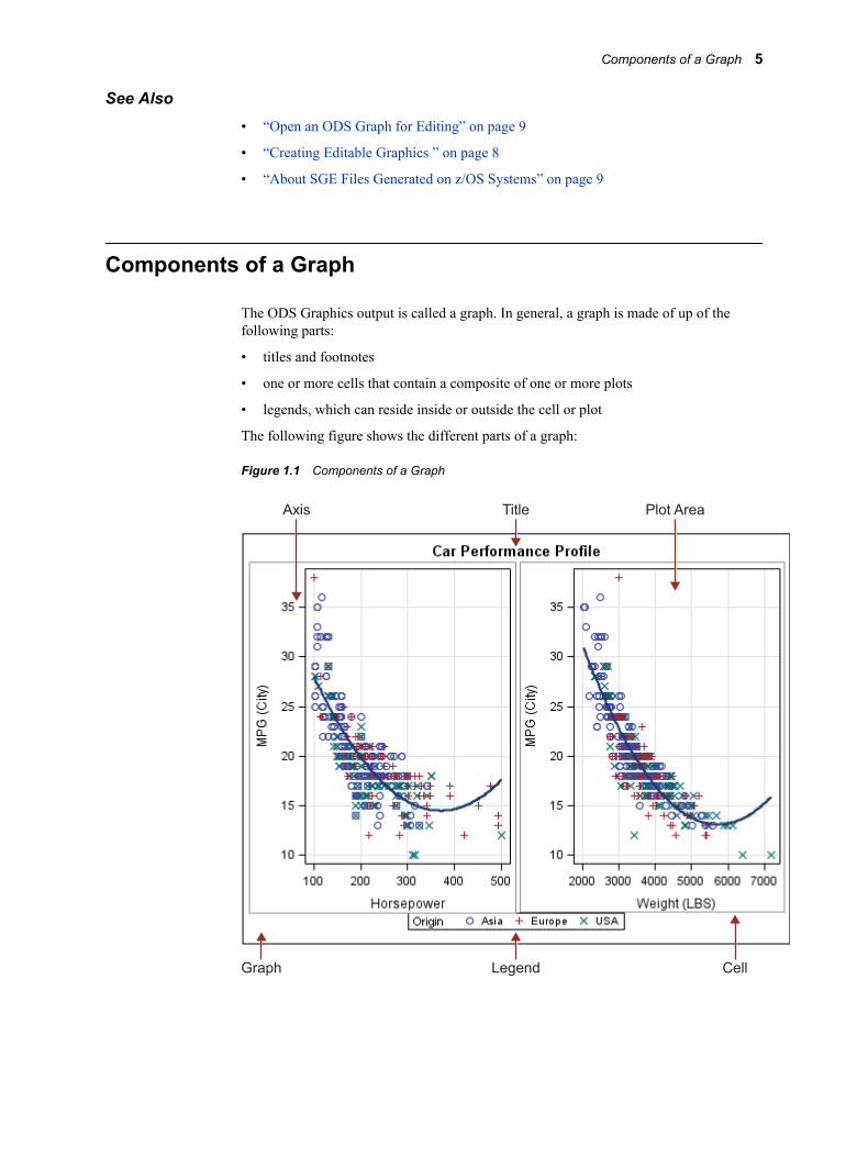
The ODS Graphics output is called a graph. In general, a graph is made of up of thefollowing parts:
• titles and footnotes
• one or more cells that contain a composite of one or more plots
• legends, which can reside inside or outside the cell or plot
The following figure shows the different parts of a graph:
Figure 1.1 Components of a Graph
Axis
Graph Legend Cell
Title Plot Area
Components of a Graph 5
General Editing and Annotation Concepts
You can edit and annotate graphs. Editing and annotating tasks differ from each other inthe following ways:
• When you edit a graph, you edit elements of the graph such as the title, footnote, orlegend.
You can also change the visual characteristics of the plots, such as the colors ofmarkers and lines. You can change the style applied to a graph, and you can resizethe graph.
Some of these edits can cause the layout of the graph to change.
• When you annotate a graph, you add objects on top of the original graph. You canadd text, lines, arrows, ovals, rectangles, images, and markers. Annotation objectsare rendered in a separate layer on top of the graphical elements and do not causeany changes to the layout of the graph.
Annotation objects can be attached to graph data so that, if the graph is resized, theannotations move with the data. For more information, “Understanding AnnotationObjects and Data” on page 45.
• You can edit Graph Template Language (GTL) annotations (DRAW statements) thatare part of the original graph, as well as annotations that were created with the ODSGraphics procedures. These edits do not cause any changes to the layout of thegraph.
Use of LocaleThe ODS Graphics Editor uses the system locale, but the graph itself uses the SASlocale. For example, if the axis label is present, the label is shown in the language thatSAS uses.
6 Chapter 1 • Overview of the ODS Graphics Editor
Chapter 2
Getting Started with the ODSGraphics Editor
Using a Stand-Alone ODS Graphics Editor . . . . . . . . . . . . . . . . . . . . . . . . . . . . . . . . . 7Download and Install the Stand-Alone ODS Graphics Editor . . . . . . . . . . . . . . . . . . 7Start the Stand-Alone ODS Graphics Editor . . . . . . . . . . . . . . . . . . . . . . . . . . . . . . . 8
Creating Editable Graphics . . . . . . . . . . . . . . . . . . . . . . . . . . . . . . . . . . . . . . . . . . . . . . 8
Open an ODS Graph for Editing . . . . . . . . . . . . . . . . . . . . . . . . . . . . . . . . . . . . . . . . . 9
About SGE Files Generated on z/OS Systems . . . . . . . . . . . . . . . . . . . . . . . . . . . . . . . 9
About the Graph Toolbar . . . . . . . . . . . . . . . . . . . . . . . . . . . . . . . . . . . . . . . . . . . . . . 10
Save Graph Output . . . . . . . . . . . . . . . . . . . . . . . . . . . . . . . . . . . . . . . . . . . . . . . . . . . . 11
Print Graph Output . . . . . . . . . . . . . . . . . . . . . . . . . . . . . . . . . . . . . . . . . . . . . . . . . . . 11
Copy and Paste a Graph . . . . . . . . . . . . . . . . . . . . . . . . . . . . . . . . . . . . . . . . . . . . . . . 12
Create a New Blank Window . . . . . . . . . . . . . . . . . . . . . . . . . . . . . . . . . . . . . . . . . . . . 12
Using a Stand-Alone ODS Graphics Editor
Download and Install the Stand-Alone ODS Graphics Editor
On Windows and Linux operating systems, you can run the ODS Graphics Editor as astand-alone product without invoking SAS. You can download the stand-alone editor forfree from SAS.
To download the stand-alone ODS Graphics Editor:
1. Go to the Base SAS download site:
http://www.sas.com/apps/demosdownloads/setupcat.jsp?cat=Base+SAS+Software
2. Click the ODS Graphics Editor from the list. The ODS Graphics Editor DownloadPackages page appears.
3. View the README file for the appropriate platform. You might print the file so thatyou can refer to it later.
Note: Verify that you have the correct Java Runtime Environment installed, asspecified in the README file.
4. Select Request Download.
7
5. Read the license agreement and then click I Accept. The Download page appears.
6. Click the Download button next to the file that you want to download. Thecompressed file is downloaded to your system.
7. Follow the instructions in the README file to unpack the files, start the SASDeployment Wizard, and install the editor.
Start the Stand-Alone ODS Graphics Editor
On a Windows system, start the editor from the Windows Start menu.
To start the editor on Linux systems, follow the instructions in the editor's READMEfile.
After you start the editor, you can select File ð Open from the main menu and select anSGE file that you want to edit.
Creating Editable Graphics
You must create editable graph output before you can use the ODS Graphics Editor toedit the graph output. You can create editable graph output with a wide variety of SASprocedures.
To enable the creation of an editable graph, do the following in your SAS program:
• Make sure either the LISTING or the HTML ODS destination is open. If both areclosed, no editable graph can be produced. Both can be open. Other destinations canbe open as well.
• Add the SGE=ON option to the ODS destination statement.
Here is the general form of the SGE option:
sge = on|off|yes|no
Here is an example of its usage in an ODS LISTING statement:
ods listing sge = on;
• If needed, activate the ODS Graphics environment with the ODS GRAPHICS ONstatement. This is not required for the SAS ODS Graphics procedures (SGDESIGN,SGPLOT, SGPANEL, SGSCATTER, or SGRENDER). In addition, SAS proceduresthat support ODS produce ODS Graphics output by default when they are executedin the SAS Windowing Environment.
For more information, see “Procedures That Support ODS Graphics” in SAS/STAT9.3 User’s Guide.
When you execute the SAS program, SAS creates an ODS Graphics Editor (SGE) filealong with the graph image file. You can then open the SGE file from the Resultswindow. For details, see “Open an ODS Graph for Editing” on page 9.
Note: You cannot open an SGE file on z/OS systems. For more information, see “AboutSGE Files Generated on z/OS Systems” on page 9.
If you later change and rerun the SAS program, SAS creates a new SGE file. Theoriginal SGE file remains in the SAS Results window.
8 Chapter 2 • Getting Started with the ODS Graphics Editor
You can create editable graphs for multiple ODS destinations. Each editable graph has aunique name based on the name of the corresponding PNG file. For example, if youspecify SGE=ON for the LISTING, PDF, and HTML destinations, your editable graphswould have names such as SGPlot.sge, SGPlot_PDF.sge, and SGPlot_HTML.sge.
To disable the creation of editable graphs, add the SGE=OFF option to the ODSdestination. For example, you might submit the following code in your program:
ods listing sge = off;
Alternatively, you can close and then reopen the ODS destination.
Open an ODS Graph for EditingFrom the SAS Results window, you can open an editable graph that has been createdfrom a SAS program. For more information about editable graphs, see “CreatingEditable Graphics ” on page 8.
Note: You cannot edit an ODS graph on z/OS systems.
To open an editable graph from the SAS Results window:
1. Click the expansion icon in the SAS Results window to expand the list of graphs thatyou created.
2. Double-click the SGE file, which is identified by the icon.
The ODS Graphics Editor opens and displays the graph for editing. You can nowedit the graph using the various interactive tools.
Once the ODS Graphics Editor is open, you can open an editable graph by selecting Fileð Open from the main menu.
You can open and edit any SGE graph file. See “Types of Files That Can Be Edited” onpage 4. This includes SGE files that were created on z/OS systems, which do not supportrunning the ODS Graphics Editor. For more information, see “About SGE FilesGenerated on z/OS Systems” on page 9.
You can also select File ð New to create a blank window. You can then add annotationsto the window.
About SGE Files Generated on z/OS SystemsThe ODS Graphics Editor is a graphical application and, therefore, does not run on z/OSsystems. You cannot edit graphs on z/OS, either from the SAS Results window or in thestand-alone editor. However, you can generate SGE files on z/OS, and then move thefiles to another system on which you can run the editor (Windows, Linux, or UNIX).Then you can start the editor and edit the SGE files that you moved. For moreinformation about generating SGE files, see “Creating Editable Graphics ” on page 8.
When you generate SGE files on z/OS, SAS always writes the SGE files to the UNIXfile system (UFS). The z/OS FILESYSTEM= setting is ignored for writing SGE files.You must be authorized to create UFS files in your environment in order to generate theSGE files.
About SGE Files Generated on z/OS Systems 9
Note: SGE files can be rendered on z/OS systems using the SGRENDER procedure. Formore information, see SAS ODS Graphics: Procedures Guide.
About the Graph Toolbar
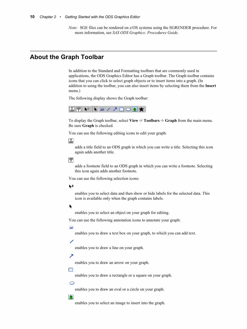
In addition to the Standard and Formatting toolbars that are commonly used inapplications, the ODS Graphics Editor has a Graph toolbar. The Graph toolbar containsicons that you can click to select graph objects or to insert items into a graph. (Inaddition to using the toolbar, you can also insert items by selecting them from the Insertmenu.)
The following display shows the Graph toolbar:
To display the Graph toolbar, select View ð Toolbars ð Graph from the main menu.Be sure Graph is checked.
You can use the following editing icons to edit your graph:
adds a title field to an ODS graph in which you can write a title. Selecting this iconagain adds another title.
adds a footnote field to an ODS graph in which you can write a footnote. Selectingthis icon again adds another footnote.
You can use the following selection icons:
enables you to select data and then show or hide labels for the selected data. Thisicon is available only when the graph contains labels.
enables you to select an object on your graph for editing.
You can use the following annotation icons to annotate your graph:
enables you to draw a text box on your graph, to which you can add text.
enables you to draw a line on your graph.
enables you to draw an arrow on your graph.
enables you to draw a rectangle or a square on your graph.
enables you to draw an oval or a circle on your graph.
enables you to select an image to insert into the graph.
10 Chapter 2 • Getting Started with the ODS Graphics Editor
places a marker at a place that you select on your graph. As shown here, the currentmarker setting displays as a star. The icon in your operating environment might bedifferent.
Save Graph Output
To save graph output:
1. Select File ð Save As from the menu.
2. Select the directory where you want the graph to be saved. The default location is thecurrent directory for the SAS program that generated the SGE file.
3. Select the type of file to save.
• If you save the file in SGE format, then you can later reopen and edit the file.
• If you save the file in PNG format, then the graph is saved as a flat image. Thegraph in this format cannot be edited, though it can be annotated.
You can change the resolution by modifying the dots per inches (DPI). Changingthe DPI affects only the image. The actual graph continues to display with 100DPI.
If you specify a DPI larger than 100, the graph image is resized. Any annotationthat is not attached to the data retains its original position after the layoutchanges. For an example that illustrates this behavior, see “Example: AnnotationPositioned Over a Legend in a Graph That Is Resized” on page 55. (For moreinformation about attachment to data, see “Understanding Annotation Objectsand Data” on page 45.)
The maximum value that you can specify is 300 DPI. If you want to obtain ahigher resolution, you can render the SGE file using the SGRENDER procedureand specify a DPI value in an ODS statement. For more information about theSGRENDER procedure, see SAS ODS Graphics: Procedures Guide.
4. Enter the name of the graph in the File name field.
5. Click Save.
The Save operation does not affect the graph output in the Results window in SAS.
Print Graph Output
You can print SGE and PNG files from the ODS Graphics Editor. You can also include aPNG file in a PDF document and then print the PDF document.
To print a graph from the ODS Graphics Editor:
1. Select File ð Print from the menu.
2. Select print options from the Print window.
3. Click OK.
Print Graph Output 11
You can select File ð Print Preview to preview your graph before you print it.
Copy and Paste a Graph
Graph output can be copied to the system clipboard to use in another document.
To copy and paste a graph:
1. Open the graph that you want to copy.
2. Select Edit ð Copy View from the main menu.
You can paste the graph into the target application using that application's pastecommand.
Create a New Blank WindowYou can select File ð New to create a blank window. You can then add annotations tothe window.
12 Chapter 2 • Getting Started with the ODS Graphics Editor
Part 2
Editing Graphs
Chapter 3Modifying General Graph Properties . . . . . . . . . . . . . . . . . . . . . . . . . . . . . 15
Chapter 4Working with Titles and Footnotes . . . . . . . . . . . . . . . . . . . . . . . . . . . . . . . 19
Chapter 5Working with Legends . . . . . . . . . . . . . . . . . . . . . . . . . . . . . . . . . . . . . . . . . . . 27
Chapter 6Modifying Plot and Axis Properties . . . . . . . . . . . . . . . . . . . . . . . . . . . . . . . 31
Chapter 7Working with Data Labels and Multi-Cell Graphs . . . . . . . . . . . . . . . . . 39
13

14
Chapter 3
Modifying General GraphProperties
Specify a Style for a Graph . . . . . . . . . . . . . . . . . . . . . . . . . . . . . . . . . . . . . . . . . . . . . 15
Resize a Graph . . . . . . . . . . . . . . . . . . . . . . . . . . . . . . . . . . . . . . . . . . . . . . . . . . . . . . . 16
Change the Background Color of a Graph . . . . . . . . . . . . . . . . . . . . . . . . . . . . . . . . 17
Specify a Style for a Graph
Styles control the overall visual appearance of graphs. Styles specify colors, fonts, linestyles, and other attributes of graph elements. You can change the appearance of yourgraph by selecting one of the styles that are provided. For example, you can change thestyle of a graph from the Default style to the Journal style if the graph is intended forgray-scale publications.
By default, graph SGE files use the active ODS destination style that is specified in theSAS program. For example, you can specify the Analysis style using the followingstatement in the program:
ods listing sge=on style=Analysis;
To select a style:
1. With your graph displayed, select Format ð Style from the main menu.
2. From the cascading menu, select a graph style.
You can select one of the following styles:
Analysisis a color style recommended for output in Web pages or for color print media. Thisstyle might not display well in gray-scale output.
Defaultis a color style intended for general-purpose work. This style is designed todiscriminate among groups in both color and gray-scale output.
HTMLBlueCMLis a color style recommended for output in Web pages or for color print media. Thisstyle has a white background and has been optimized for HTML output.
Journalis a gray-scale style recommended for journal articles and other publications that areprinted in gray scale.
15
Listingis similar to Default but has a white background. This style is used by SAS for listingoutput.
Statisticalis a color style recommended for output in Web pages or for color print media. Thisstyle might not display well on devices that produce gray-scale output.
StatGraphSchemeis the default style for all SGE files. This style inherits attributes from the style thatwas used when the graph was created.
Various elements of the graph derive their visual attributes, such as color, from specificstyle elements. Individual property settings override the style elements. For example, ifyou have assigned an overriding color to an object in the graph, then selecting a differentstyle retains the overriding value that has been assigned.
Resize a Graph
When you resize a graph, you can then print or save the graph in its new size.
If you resize a graph and there is not enough space to display entire titles, footnotes, oraxis labels, then an alternate short label is displayed. For details, see “Use of AlternateShort Text in Graph Elements ” on page 25 .
To resize a graph:
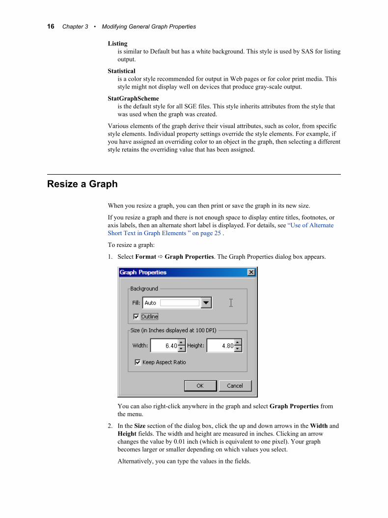
1. Select Format ð Graph Properties. The Graph Properties dialog box appears.
You can also right-click anywhere in the graph and select Graph Properties fromthe menu.
2. In the Size section of the dialog box, click the up and down arrows in the Width andHeight fields. The width and height are measured in inches. Clicking an arrowchanges the value by 0.01 inch (which is equivalent to one pixel). Your graphbecomes larger or smaller depending on which values you select.
Alternatively, you can type the values in the fields.
16 Chapter 3 • Modifying General Graph Properties
Note: To resize the graph proportionally, make sure the Keep Aspect Ratio checkbox is checked. If you want to specify the width and height independentlywithout retaining the current aspect ratio, then clear the check box.
3. Click OK.
Note: You can also enlarge or reduce the view of a graph by using the Zoom tool. TheZoom tool does not resize the graph. To zoom in or out, select View ð Zoom fromthe menu, and then select the zoom value that you want.
Change the Background Color of a Graph
To change the background color of a graph:
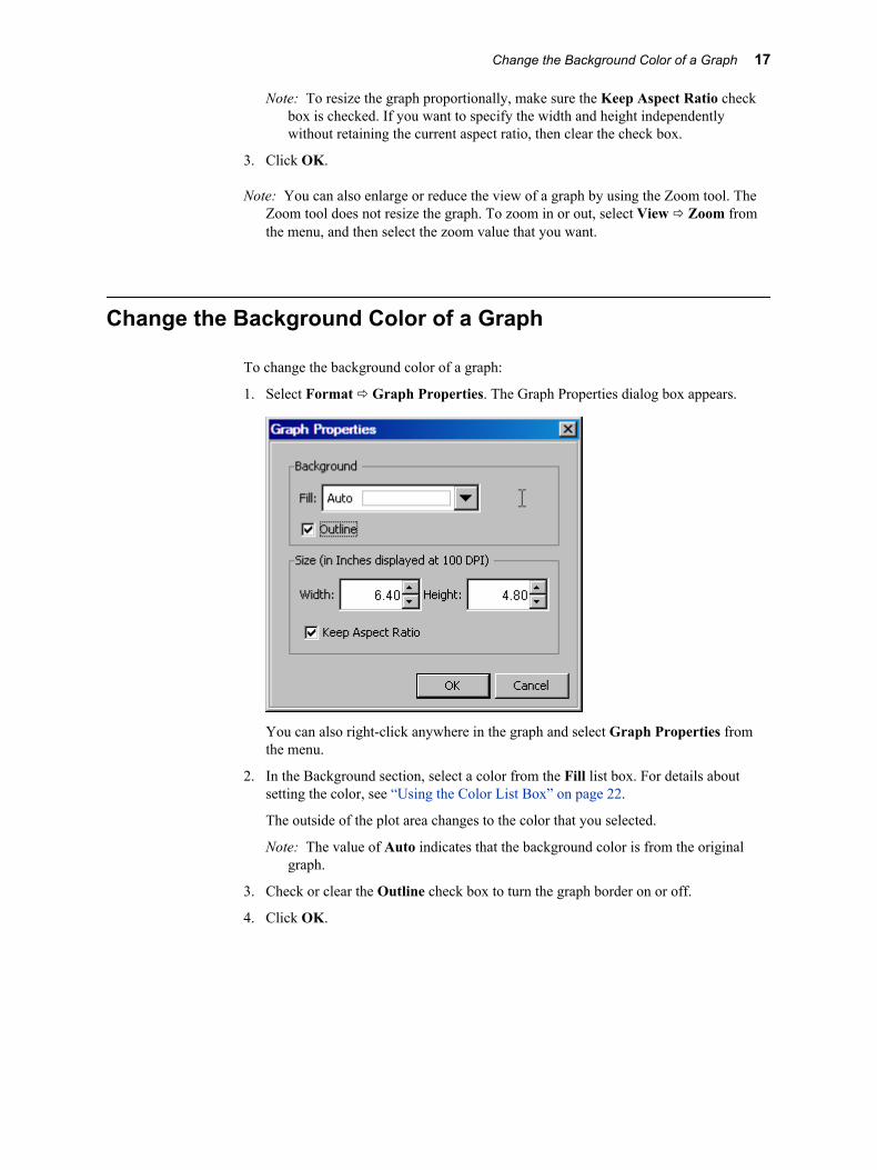
1. Select Format ð Graph Properties. The Graph Properties dialog box appears.
You can also right-click anywhere in the graph and select Graph Properties fromthe menu.
2. In the Background section, select a color from the Fill list box. For details aboutsetting the color, see “Using the Color List Box” on page 22.
The outside of the plot area changes to the color that you selected.
Note: The value of Auto indicates that the background color is from the originalgraph.
3. Check or clear the Outline check box to turn the graph border on or off.
4. Click OK.
Change the Background Color of a Graph 17

18 Chapter 3 • Modifying General Graph Properties
Chapter 4
Working with Titles and Footnotes
About Titles and Footnotes . . . . . . . . . . . . . . . . . . . . . . . . . . . . . . . . . . . . . . . . . . . . . 19
Add a Title or Footnote to a Graph . . . . . . . . . . . . . . . . . . . . . . . . . . . . . . . . . . . . . . 19
Edit or Format a Title or Footnote . . . . . . . . . . . . . . . . . . . . . . . . . . . . . . . . . . . . . . . 20
Using the Formatting Toolbar . . . . . . . . . . . . . . . . . . . . . . . . . . . . . . . . . . . . . . . . . . . 21
Using the Color List Box . . . . . . . . . . . . . . . . . . . . . . . . . . . . . . . . . . . . . . . . . . . . . . . 22
Aligning a Title or Footnote in a Graph . . . . . . . . . . . . . . . . . . . . . . . . . . . . . . . . . . . 23Alignment of Titles and Footnotes . . . . . . . . . . . . . . . . . . . . . . . . . . . . . . . . . . . . . . 23Align a Title or Footnote . . . . . . . . . . . . . . . . . . . . . . . . . . . . . . . . . . . . . . . . . . . . . 24
Move a Title or Footnote in a Graph . . . . . . . . . . . . . . . . . . . . . . . . . . . . . . . . . . . . . 24
Delete a Title or Footnote from a Graph . . . . . . . . . . . . . . . . . . . . . . . . . . . . . . . . . . 25
Use of Alternate Short Text in Graph Elements . . . . . . . . . . . . . . . . . . . . . . . . . . . . 25
About Titles and Footnotes
You can add multiple titles and footnotes to a graph. The limit to the number of titles orfootnotes that you can add depends on the size of your graph. As you add more titles orfootnotes, the Y axis of the graph shrinks proportionally to the point where the graph isno longer visible.
When you add a long title or footnote to a graph, the text automatically wraps to the nextline. If you move a title or footnote to a different location in the graph, all of the lines ofa single title or footnote move as one unit.
Both titles and footnotes support rich text editing.
Note: In addition to titles and footnotes, some graphs might have been created withother text entries. You can edit any text entry that was defined as editable in thegraph.
Add a Title or Footnote to a GraphTo add a title or footnote to a graph:
19
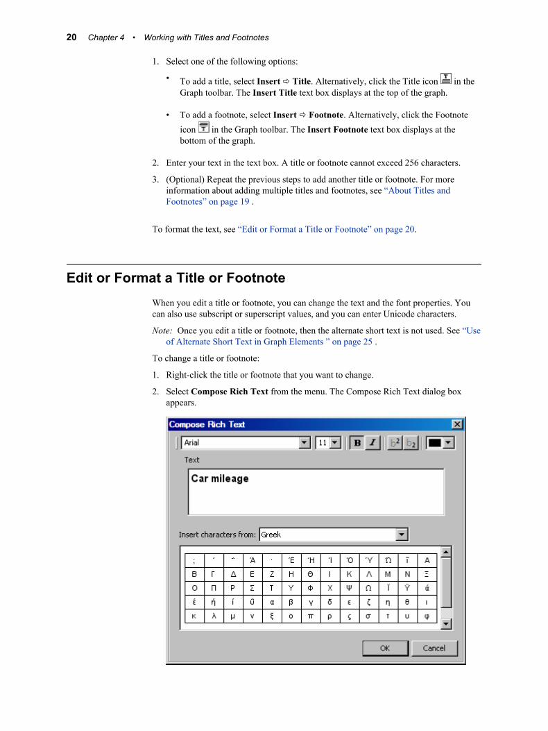
1. Select one of the following options:
• To add a title, select Insert ð Title. Alternatively, click the Title icon in theGraph toolbar. The Insert Title text box displays at the top of the graph.
• To add a footnote, select Insert ð Footnote. Alternatively, click the Footnoteicon in the Graph toolbar. The Insert Footnote text box displays at thebottom of the graph.
2. Enter your text in the text box. A title or footnote cannot exceed 256 characters.
3. (Optional) Repeat the previous steps to add another title or footnote. For moreinformation about adding multiple titles and footnotes, see “About Titles andFootnotes” on page 19 .
To format the text, see “Edit or Format a Title or Footnote” on page 20.
Edit or Format a Title or FootnoteWhen you edit a title or footnote, you can change the text and the font properties. Youcan also use subscript or superscript values, and you can enter Unicode characters.
Note: Once you edit a title or footnote, then the alternate short text is not used. See “Useof Alternate Short Text in Graph Elements ” on page 25 .
To change a title or footnote:
1. Right-click the title or footnote that you want to change.
2. Select Compose Rich Text from the menu. The Compose Rich Text dialog boxappears.
20 Chapter 4 • Working with Titles and Footnotes
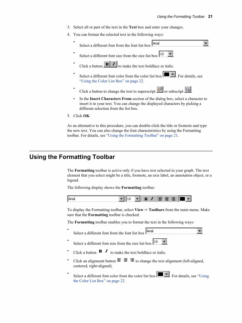
3. Select all or part of the text in the Text box and enter your changes.
4. You can format the selected text in the following ways:
•Select a different font from the font list box .
•Select a different font size from the size list box .
•Click a button to make the text boldface or italic.
•Select a different font color from the color list box . For details, see“Using the Color List Box” on page 22.
•Click a button to change the text to superscript or subscript .
• In the Insert Characters From section of the dialog box, select a character toinsert it in your text. You can change the displayed characters by picking adifferent selection from the list box.
5. Click OK.
As an alternative to this procedure, you can double-click the title or footnote and typethe new text. You can also change the font characteristics by using the Formattingtoolbar. For details, see “Using the Formatting Toolbar” on page 21.
Using the Formatting Toolbar
The Formatting toolbar is active only if you have text selected in your graph. The textelement that you select might be a title, footnote, an axis label, an annotation object, or alegend.
The following display shows the Formatting toolbar:
To display the Formatting toolbar, select View ð Toolbars from the main menu. Makesure that the Formatting toolbar is checked.
The Formatting toolbar enables you to format the text in the following ways:
•Select a different font from the font list box .
•Select a different font size from the size list box .
• Click a button to make the text boldface or italic.
• Click an alignment button to change the text alignment (left-aligned,centered, right-aligned).
•Select a different font color from the color list box . For details, see “Usingthe Color List Box” on page 22.
Using the Formatting Toolbar 21
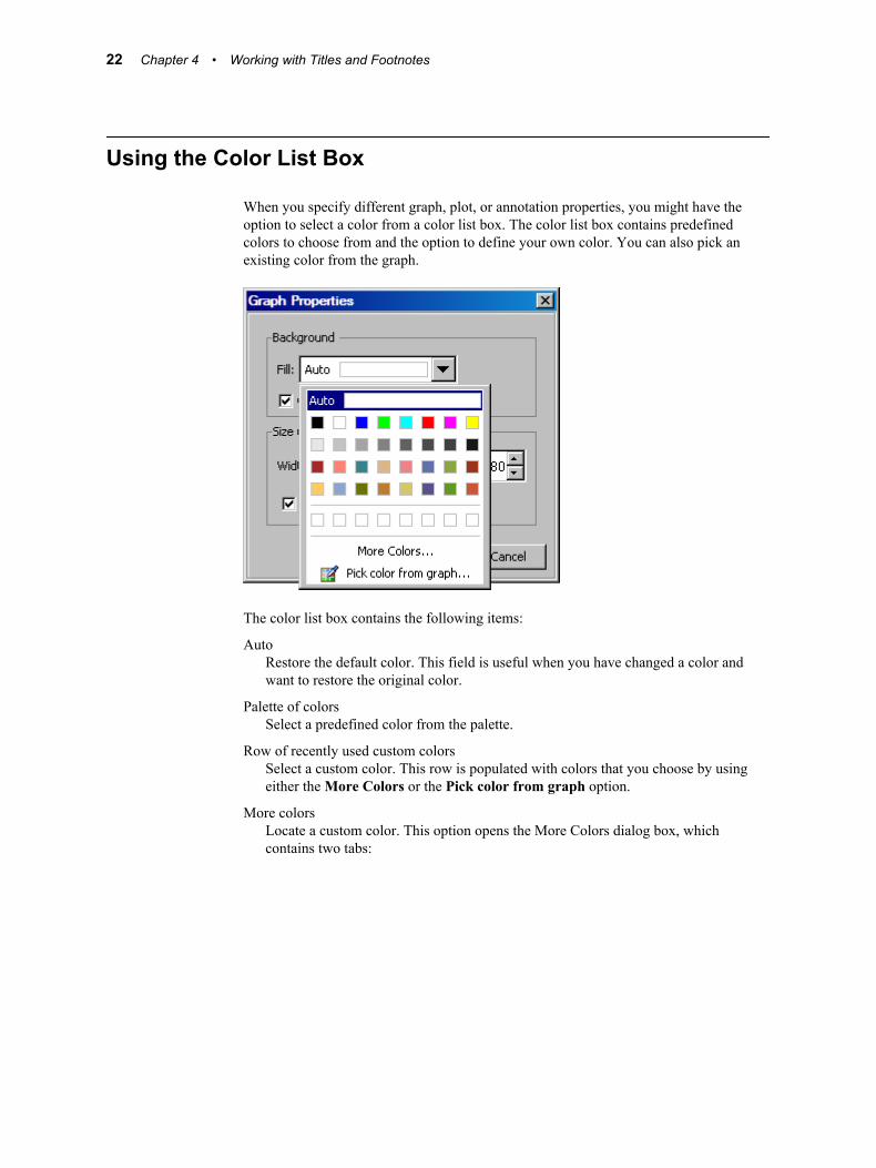
Using the Color List Box
When you specify different graph, plot, or annotation properties, you might have theoption to select a color from a color list box. The color list box contains predefinedcolors to choose from and the option to define your own color. You can also pick anexisting color from the graph.
The color list box contains the following items:
AutoRestore the default color. This field is useful when you have changed a color andwant to restore the original color.
Palette of colorsSelect a predefined color from the palette.
Row of recently used custom colorsSelect a custom color. This row is populated with colors that you choose by usingeither the More Colors or the Pick color from graph option.
More colorsLocate a custom color. This option opens the More Colors dialog box, whichcontains two tabs:
22 Chapter 4 • Working with Titles and Footnotes
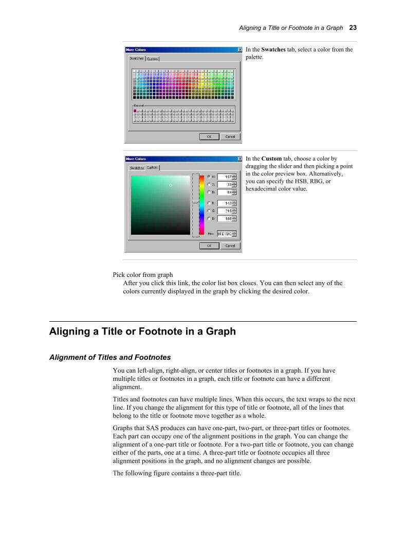
In the Swatches tab, select a color from thepalette.
In the Custom tab, choose a color bydragging the slider and then picking a pointin the color preview box. Alternatively,you can specify the HSB, RBG, orhexadecimal color value.
Pick color from graphAfter you click this link, the color list box closes. You can then select any of thecolors currently displayed in the graph by clicking the desired color.
Aligning a Title or Footnote in a Graph
Alignment of Titles and FootnotesYou can left-align, right-align, or center titles or footnotes in a graph. If you havemultiple titles or footnotes in a graph, each title or footnote can have a differentalignment.
Titles and footnotes can have multiple lines. When this occurs, the text wraps to the nextline. If you change the alignment for this type of title or footnote, all of the lines thatbelong to the title or footnote move together as a whole.
Graphs that SAS produces can have one-part, two-part, or three-part titles or footnotes.Each part can occupy one of the alignment positions in the graph. You can change thealignment of a one-part title or footnote. For a two-part title or footnote, you can changeeither of the parts, one at a time. A three-part title or footnote occupies all threealignment positions in the graph, and no alignment changes are possible.
The following figure contains a three-part title.
Aligning a Title or Footnote in a Graph 23
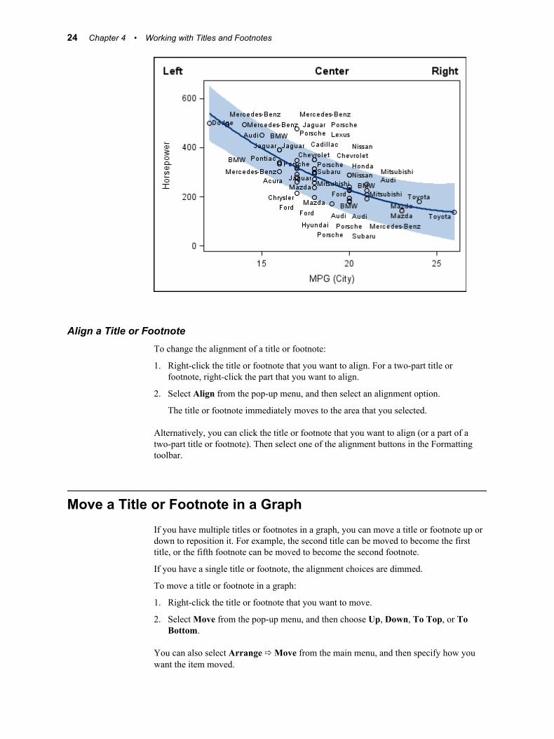
Align a Title or FootnoteTo change the alignment of a title or footnote:
1. Right-click the title or footnote that you want to align. For a two-part title orfootnote, right-click the part that you want to align.
2. Select Align from the pop-up menu, and then select an alignment option.
The title or footnote immediately moves to the area that you selected.
Alternatively, you can click the title or footnote that you want to align (or a part of atwo-part title or footnote). Then select one of the alignment buttons in the Formattingtoolbar.
Move a Title or Footnote in a GraphIf you have multiple titles or footnotes in a graph, you can move a title or footnote up ordown to reposition it. For example, the second title can be moved to become the firsttitle, or the fifth footnote can be moved to become the second footnote.
If you have a single title or footnote, the alignment choices are dimmed.
To move a title or footnote in a graph:
1. Right-click the title or footnote that you want to move.
2. Select Move from the pop-up menu, and then choose Up, Down, To Top, or ToBottom.
You can also select Arrange ð Move from the main menu, and then specify how youwant the item moved.
24 Chapter 4 • Working with Titles and Footnotes
Titles and footnotes can have up to three parts, one for each alignment position (left,center, right). You cannot move the individual part of multi-part title or footnote. Thewhole title or footnote moves together. (For more information about alignment, see “Aligning a Title or Footnote in a Graph” on page 23 .)
Delete a Title or Footnote from a GraphTo delete a title or footnote in a graph:
1. Right-click the title or footnote that you want to delete.
2. Select Delete from the pop-up menu.
Note: To undo the change, select Edit ð Undo from the menu.
For multi-part titles and footnotes, you can delete one part at a time.
Use of Alternate Short Text in Graph ElementsIn addition to the standard text that is displayed, titles, footnotes, and axis labels havealternate short text. This short text is specified as a GTL option in the SAS program thatdefines the graph.
If there is not enough space to display the standard text, then the short text is displayed.For example, if you resize a graph and there is not enough space to display the wholeaxis label, then the short axis label is displayed. If you later enlarge the graph so thatenough space is made available, then the long label is displayed.
You can override the short text by changing the text of the title, footnote, or axis label.Once you change the text, then only the new modified text is displayed regardless of thesize of the graph.
Use of Alternate Short Text in Graph Elements 25

26 Chapter 4 • Working with Titles and Footnotes
Chapter 5
Working with Legends
Add or Edit a Legend Title . . . . . . . . . . . . . . . . . . . . . . . . . . . . . . . . . . . . . . . . . . . . . 27
Change the Outline and Background Color of a Legend . . . . . . . . . . . . . . . . . . . . . 27
Move a Legend Inside or Outside a Plot . . . . . . . . . . . . . . . . . . . . . . . . . . . . . . . . . . . 28
Add or Edit a Legend TitleYou cannot add or delete a legend. You also cannot edit the labels in the legend. Youcan, however, add or edit the title of the legend.
To add or edit a legend title:
1. Right-click the legend and select Add (Edit) Title from the pop-up menu. A Legendtext box appears next to the legend.
2. In the text box, enter the text that you want for the title. The title cannot exceed 256characters.
3. To change the font characteristics, select the title text and use the Formatting toolbar.For details, see “Using the Formatting Toolbar” on page 21.
Change the Outline and Background Color of aLegend
To change the outline and fill color of a legend:
1. Right-click the legend and select Legend Properties from the pop-up menu. TheLegend Properties dialog box appears.
27
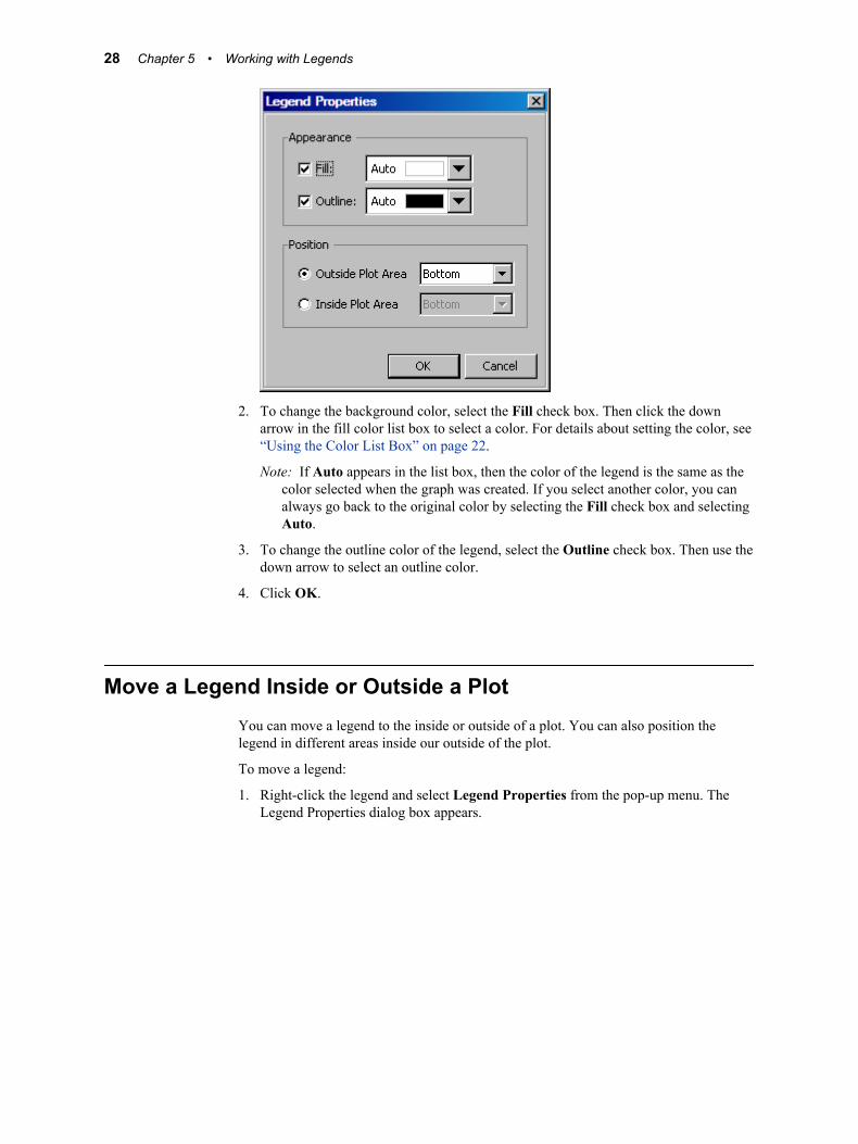
2. To change the background color, select the Fill check box. Then click the downarrow in the fill color list box to select a color. For details about setting the color, see“Using the Color List Box” on page 22.
Note: If Auto appears in the list box, then the color of the legend is the same as thecolor selected when the graph was created. If you select another color, you canalways go back to the original color by selecting the Fill check box and selectingAuto.
3. To change the outline color of the legend, select the Outline check box. Then use thedown arrow to select an outline color.
4. Click OK.
Move a Legend Inside or Outside a PlotYou can move a legend to the inside or outside of a plot. You can also position thelegend in different areas inside our outside of the plot.
To move a legend:
1. Right-click the legend and select Legend Properties from the pop-up menu. TheLegend Properties dialog box appears.
28 Chapter 5 • Working with Legends
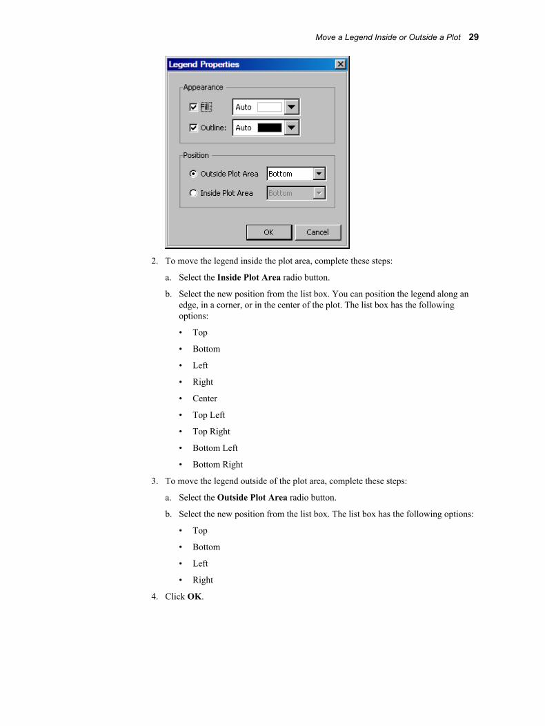
2. To move the legend inside the plot area, complete these steps:
a. Select the Inside Plot Area radio button.
b. Select the new position from the list box. You can position the legend along anedge, in a corner, or in the center of the plot. The list box has the followingoptions:
• Top
• Bottom
• Left
• Right
• Center
• Top Left
• Top Right
• Bottom Left
• Bottom Right
3. To move the legend outside of the plot area, complete these steps:
a. Select the Outside Plot Area radio button.
b. Select the new position from the list box. The list box has the following options:
• Top
• Bottom
• Left
• Right
4. Click OK.
Move a Legend Inside or Outside a Plot 29

30 Chapter 5 • Working with Legends
Chapter 6
Modifying Plot and Axis Properties
Working with Plot Properties . . . . . . . . . . . . . . . . . . . . . . . . . . . . . . . . . . . . . . . . . . . 31The Plot Properties Dialog Box . . . . . . . . . . . . . . . . . . . . . . . . . . . . . . . . . . . . . . . . 31General Properties . . . . . . . . . . . . . . . . . . . . . . . . . . . . . . . . . . . . . . . . . . . . . . . . . . 32Plot Properties . . . . . . . . . . . . . . . . . . . . . . . . . . . . . . . . . . . . . . . . . . . . . . . . . . . . . . 32Axis Properties . . . . . . . . . . . . . . . . . . . . . . . . . . . . . . . . . . . . . . . . . . . . . . . . . . . . . 35
Working with Axis Properties . . . . . . . . . . . . . . . . . . . . . . . . . . . . . . . . . . . . . . . . . . . 36
Working with Axis Labels . . . . . . . . . . . . . . . . . . . . . . . . . . . . . . . . . . . . . . . . . . . . . . 36
Edit an Existing Axis Label . . . . . . . . . . . . . . . . . . . . . . . . . . . . . . . . . . . . . . . . . . . . . 37
Add an Axis Label . . . . . . . . . . . . . . . . . . . . . . . . . . . . . . . . . . . . . . . . . . . . . . . . . . . . 37
Show or Hide an Axis Label . . . . . . . . . . . . . . . . . . . . . . . . . . . . . . . . . . . . . . . . . . . . 37
Delete an Axis Label . . . . . . . . . . . . . . . . . . . . . . . . . . . . . . . . . . . . . . . . . . . . . . . . . . . 38
Working with Plot Properties
The Plot Properties Dialog Box
You can modify all of the properties of the plots and axes that are in a cell by using thePlot Properties dialog box.
31
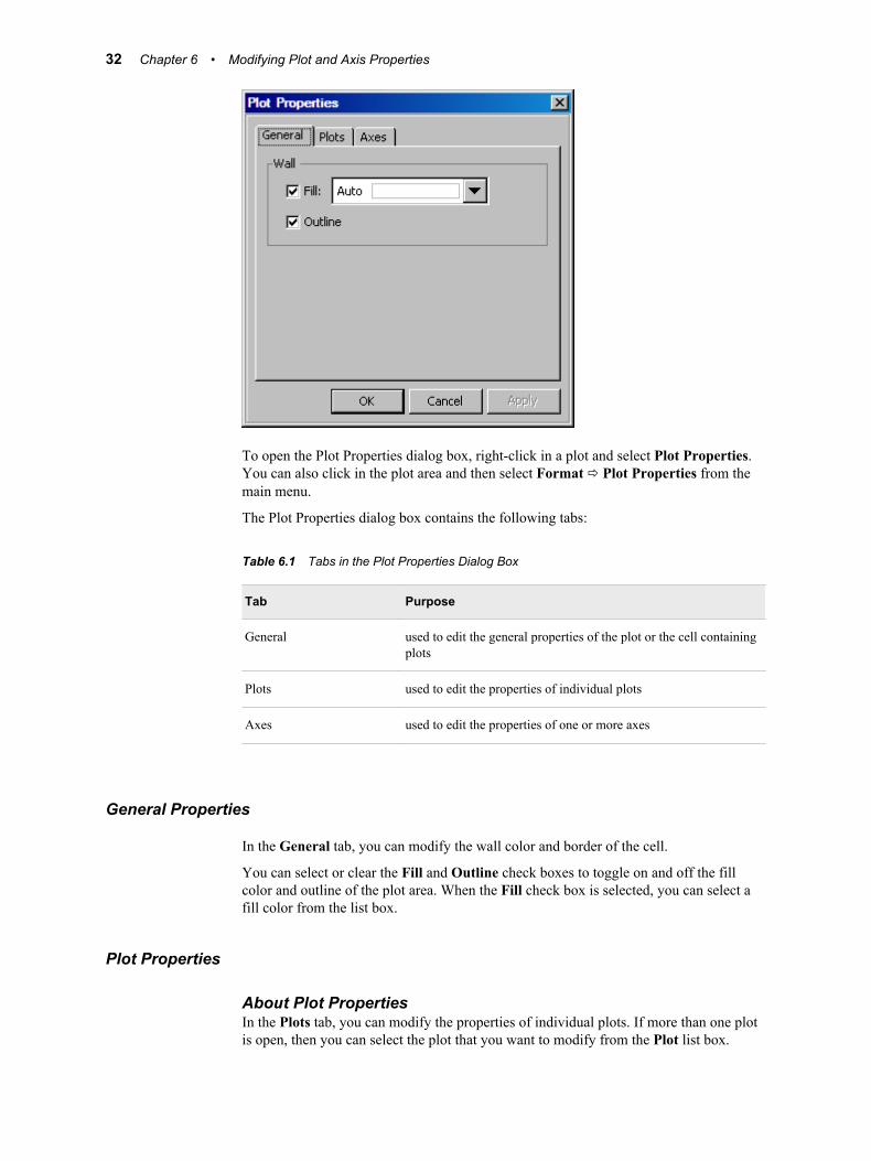
To open the Plot Properties dialog box, right-click in a plot and select Plot Properties.You can also click in the plot area and then select Format ð Plot Properties from themain menu.
The Plot Properties dialog box contains the following tabs:
Table 6.1 Tabs in the Plot Properties Dialog Box
Tab Purpose
General used to edit the general properties of the plot or the cell containingplots
Plots used to edit the properties of individual plots
Axes used to edit the properties of one or more axes
General Properties
In the General tab, you can modify the wall color and border of the cell.
You can select or clear the Fill and Outline check boxes to toggle on and off the fillcolor and outline of the plot area. When the Fill check box is selected, you can select afill color from the list box.
Plot Properties
About Plot PropertiesIn the Plots tab, you can modify the properties of individual plots. If more than one plotis open, then you can select the plot that you want to modify from the Plot list box.
32 Chapter 6 • Modifying Plot and Axis Properties
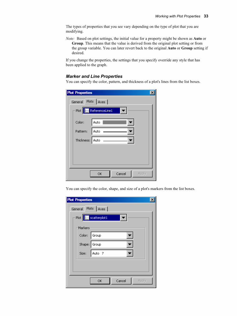
The types of properties that you see vary depending on the type of plot that you aremodifying.
Note: Based on plot settings, the initial value for a property might be shown as Auto orGroup. This means that the value is derived from the original plot setting or fromthe group variable. You can later revert back to the original Auto or Group setting ifdesired.
If you change the properties, the settings that you specify override any style that hasbeen applied to the graph.
Marker and Line PropertiesYou can specify the color, pattern, and thickness of a plot's lines from the list boxes.
You can specify the color, shape, and size of a plot's markers from the list boxes.
Working with Plot Properties 33
For markers, in addition to Auto or Group value, the initial value for any of theproperties might be as follows:
• If the MarkerColorGradient variable is defined, then Gradient is displayed as thecurrent color value. The color list is dimmed, and you cannot change the color.
• If the MarkerCharacter variable is defined, then Character is displayed as thecurrent shape. The shape and size are dimmed, and you cannot change them.
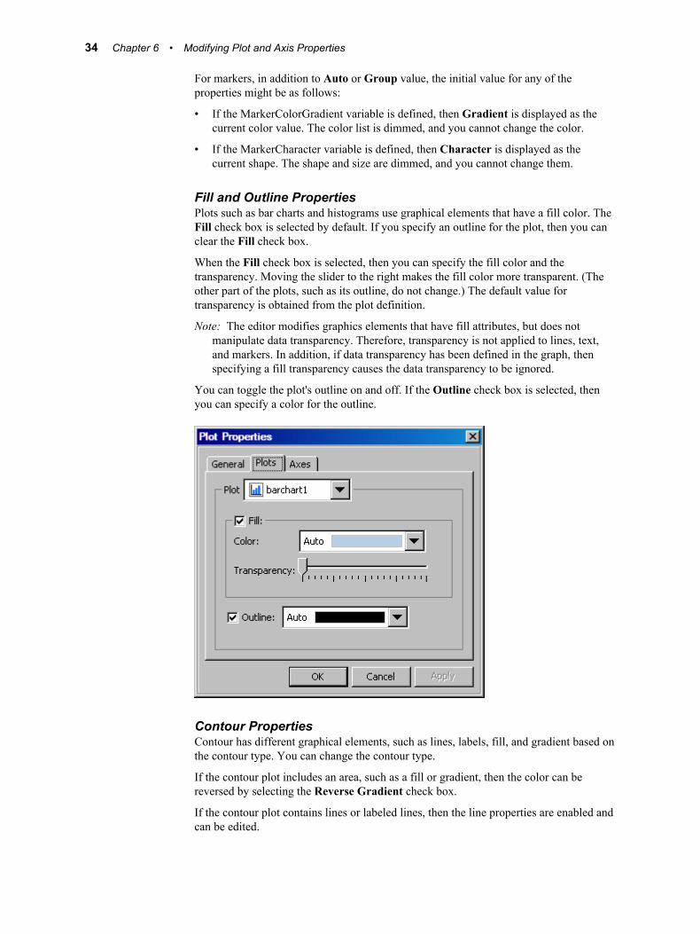
Fill and Outline PropertiesPlots such as bar charts and histograms use graphical elements that have a fill color. TheFill check box is selected by default. If you specify an outline for the plot, then you canclear the Fill check box.
When the Fill check box is selected, then you can specify the fill color and thetransparency. Moving the slider to the right makes the fill color more transparent. (Theother part of the plots, such as its outline, do not change.) The default value fortransparency is obtained from the plot definition.
Note: The editor modifies graphics elements that have fill attributes, but does notmanipulate data transparency. Therefore, transparency is not applied to lines, text,and markers. In addition, if data transparency has been defined in the graph, thenspecifying a fill transparency causes the data transparency to be ignored.
You can toggle the plot's outline on and off. If the Outline check box is selected, thenyou can specify a color for the outline.
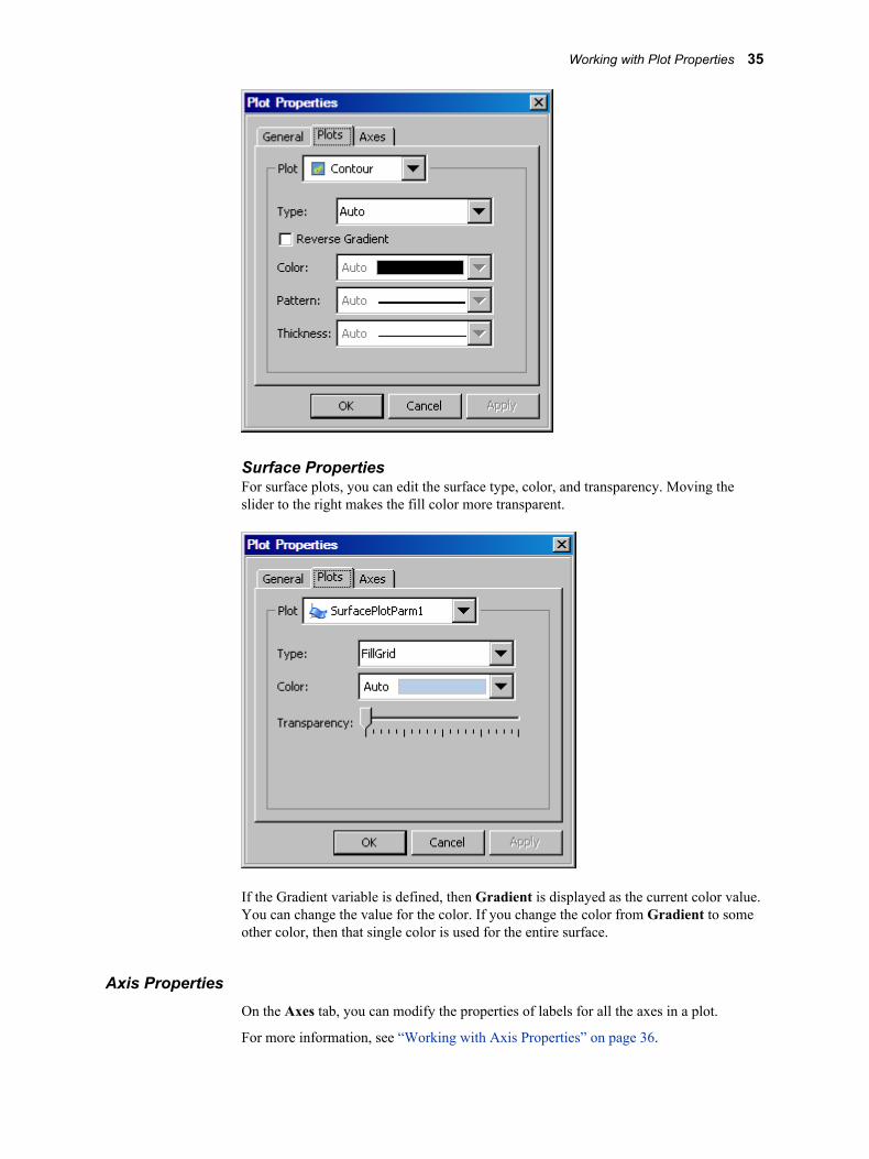
Contour PropertiesContour has different graphical elements, such as lines, labels, fill, and gradient based onthe contour type. You can change the contour type.
If the contour plot includes an area, such as a fill or gradient, then the color can bereversed by selecting the Reverse Gradient check box.
If the contour plot contains lines or labeled lines, then the line properties are enabled andcan be edited.
34 Chapter 6 • Modifying Plot and Axis Properties
Surface PropertiesFor surface plots, you can edit the surface type, color, and transparency. Moving theslider to the right makes the fill color more transparent.
If the Gradient variable is defined, then Gradient is displayed as the current color value.You can change the value for the color. If you change the color from Gradient to someother color, then that single color is used for the entire surface.
Axis PropertiesOn the Axes tab, you can modify the properties of labels for all the axes in a plot.
For more information, see “Working with Axis Properties” on page 36.
Working with Plot Properties 35
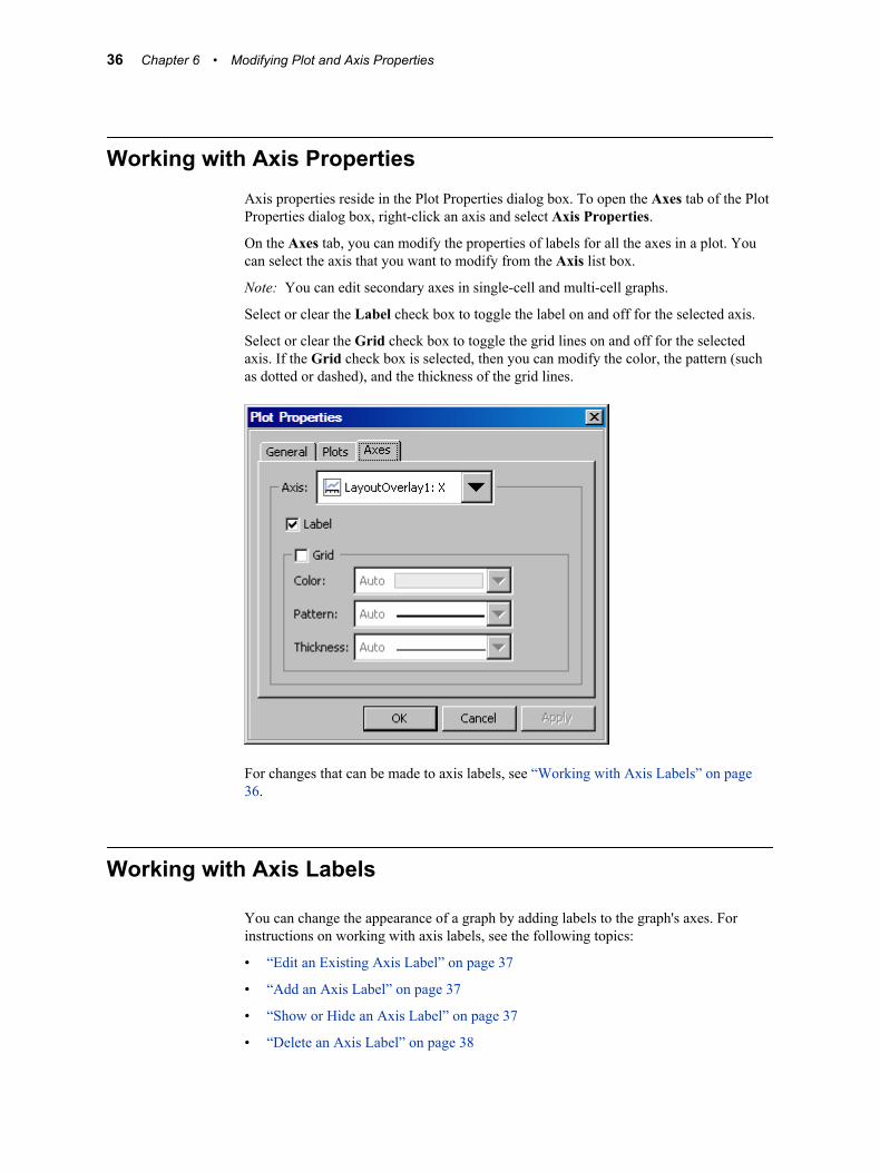
Working with Axis PropertiesAxis properties reside in the Plot Properties dialog box. To open the Axes tab of the PlotProperties dialog box, right-click an axis and select Axis Properties.
On the Axes tab, you can modify the properties of labels for all the axes in a plot. Youcan select the axis that you want to modify from the Axis list box.
Note: You can edit secondary axes in single-cell and multi-cell graphs.
Select or clear the Label check box to toggle the label on and off for the selected axis.
Select or clear the Grid check box to toggle the grid lines on and off for the selectedaxis. If the Grid check box is selected, then you can modify the color, the pattern (suchas dotted or dashed), and the thickness of the grid lines.
For changes that can be made to axis labels, see “Working with Axis Labels” on page36.
Working with Axis Labels
You can change the appearance of a graph by adding labels to the graph's axes. Forinstructions on working with axis labels, see the following topics:
• “Edit an Existing Axis Label” on page 37
• “Add an Axis Label” on page 37
• “Show or Hide an Axis Label” on page 37
• “Delete an Axis Label” on page 38
36 Chapter 6 • Modifying Plot and Axis Properties
You can also show grid lines for an axis and specify the visual properties of the gridlines. For more information, see “Axis Properties ” on page 35.
Edit an Existing Axis LabelYou can edit an existing X or Y axis label (or X,Y, and Z labels for three-dimensionalgraphs). If the same axis is displayed on both sides of the graph (right and left or top andbottom), then your edits apply to both of the axis labels.
Note: Once you edit a label, then the alternate short text is no longer used for the label.For more information, see “Use of Alternate Short Text in Graph Elements ” on page25.
To edit an axis label:
1. Double-click the axis label that you want to edit.
2. Enter or delete text in the axis label.
3. To change the font characteristics, select the label text and then use the Formattingtoolbar to make your changes. For details, see “Using the Formatting Toolbar” onpage 21.
Add an Axis LabelTo add a label to an axis:
1. Right-click along the axis where you want to add a label.
2. Select Add ('Edit') Label from the pop-up menu. A text box appears.
3. Enter the label for your axis in the text box. The label cannot exceed 256 characters.
4. To change the font characteristics, select the text and then use the Formatting toolbarto make your changes. For details, see “Using the Formatting Toolbar” on page 21.
Show or Hide an Axis LabelTo show or hide an axis label:
1. Right-click the axis label and select Axis Properties. The Plot Properties dialog boxappears with the Axes tab displayed.
Show or Hide an Axis Label 37
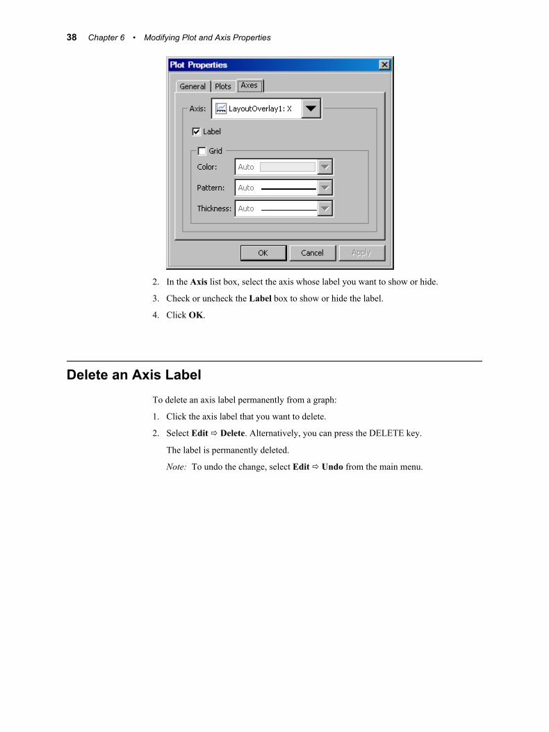
2. In the Axis list box, select the axis whose label you want to show or hide.
3. Check or uncheck the Label box to show or hide the label.
4. Click OK.
Delete an Axis LabelTo delete an axis label permanently from a graph:
1. Click the axis label that you want to delete.
2. Select Edit ð Delete. Alternatively, you can press the DELETE key.
The label is permanently deleted.
Note: To undo the change, select Edit ð Undo from the main menu.
38 Chapter 6 • Modifying Plot and Axis Properties

Chapter 7
Working with Data Labels andMulti-Cell Graphs
Display or Hide Data Labels . . . . . . . . . . . . . . . . . . . . . . . . . . . . . . . . . . . . . . . . . . . . 39
Working with Multi-Cell Graphs . . . . . . . . . . . . . . . . . . . . . . . . . . . . . . . . . . . . . . . . 40
Display or Hide Data Labels
Some plots might display data labels for each observation in the plot. If there are a lot ofobservations, then the plot can become cluttered. You can limit the display to those datalabels that are important to the analysis.
To display or hide data labels:
1. Click the data label icon in the Graph toolbar.
2. Select the observations for data label management in any of the following ways:
• Click an observation to select it. If you press CTRL and click an observation, youcan toggle the observation on and off. Pressing CTRL also enables you to selectmultiple observations.
• Click on the data label of an observation to select it.
• Click and drag to select an area within the plot. All the observations in this areaare selected. You can add more items to the selection list by pressing CTRLwhile you click and drag to select another area containing additionalobservations.
3. Right-click and select one of the following label options:
• Show Only Selected shows labels only for those data points that are currentlyselected. This option first turns off all the data labels and then displays the labelsonly for the selected data points.
• Show Selected shows labels for the data points that are selected. This optionleaves unchanged the data labels for all other data points that are not currentlyselected. For example, if you previously selected data points and set them toshow, with this option, they remain selected.
• Hide Selected hides labels for those data points that are selected.
• Show All shows labels for all the data points.
• Hide All hides labels for all the data points.
39
All items in the selection list are displayed with the selection color. If the selected item isin a scatter overlay and a marker is selected, then the marker displays with the selectioncolor. For a line overlay, if the marker is not turned on, then a temporary circle is createdand displayed with the selection color.
The layout of a plot refreshes when labels are turned off or on. If some labels are locatedaway from their data points, the labels move closer to the data points if space is madeavailable by hiding other labels.
Working with Multi-Cell Graphs
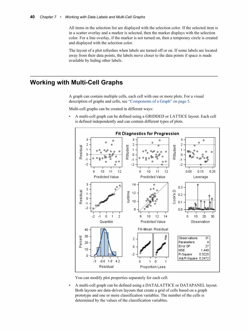
A graph can contain multiple cells, each cell with one or more plots. For a visualdescription of graphs and cells, see “Components of a Graph” on page 5.
Multi-cell graphs can be created in different ways:
• A multi-cell graph can be defined using a GRIDDED or LATTICE layout. Each cellis defined independently and can contain different types of plots.
You can modify plot properties separately for each cell.
• A multi-cell graph can be defined using a DATALATTICE or DATAPANEL layout.Both layouts are data-driven layouts that create a grid of cells based on a graphprototype and one or more classification variables. The number of the cells isdetermined by the values of the classification variables.
40 Chapter 7 • Working with Data Labels and Multi-Cell Graphs
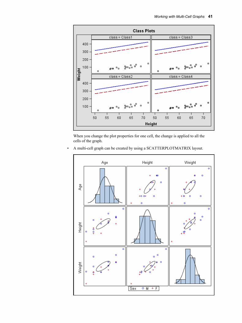
When you change the plot properties for one cell, the change is applied to all thecells of the graph.
• A multi-cell graph can be created by using a SCATTERPLOTMATRIX layout.
Working with Multi-Cell Graphs 41

Each non-diagonal cell contains the same plot types, but for a different crossing ofthe variables. When you change the plot properties for one of these cells, the changeis applied to all non-diagonal cells. (The wall and outline properties apply to allcells.)
You cannot change the properties of the following:
• the diagonal cells
• the axes
42 Chapter 7 • Working with Data Labels and Multi-Cell Graphs
Part 3
Annotating Graphs
Chapter 8Annotation Overview . . . . . . . . . . . . . . . . . . . . . . . . . . . . . . . . . . . . . . . . . . . . 45
Chapter 9Using Annotations in a Graph . . . . . . . . . . . . . . . . . . . . . . . . . . . . . . . . . . . . 61
Chapter 10Changing the Visual Properties of Annotations . . . . . . . . . . . . . . . . . . . 69
Chapter 11Adding Text to Annotations . . . . . . . . . . . . . . . . . . . . . . . . . . . . . . . . . . . . . . 75
Chapter 12Modifying Annotations . . . . . . . . . . . . . . . . . . . . . . . . . . . . . . . . . . . . . . . . . . . 79
43

44
Chapter 8
Annotation Overview
About Annotation Objects . . . . . . . . . . . . . . . . . . . . . . . . . . . . . . . . . . . . . . . . . . . . . . 45
Understanding Annotation Objects and Data . . . . . . . . . . . . . . . . . . . . . . . . . . . . . . 45
Data Attachment Examples for Annotations . . . . . . . . . . . . . . . . . . . . . . . . . . . . . . . 47Example: Text Annotation . . . . . . . . . . . . . . . . . . . . . . . . . . . . . . . . . . . . . . . . . . . . 47Example: Oval Annotation Around a Data Point . . . . . . . . . . . . . . . . . . . . . . . . . . . 48Example: Arrow Annotation Partially Attached to Data . . . . . . . . . . . . . . . . . . . . . 51Example: Marker Annotation with Text That Is Cropped . . . . . . . . . . . . . . . . . . . . 52Example: Annotation Positioned Over a Legend in a Graph That Is Resized . . . . . 55
Change the Data Attachment Properties of an Annotation . . . . . . . . . . . . . . . . . . . 57
About Annotation Objects
You can use ODS Graphics Editor to add the following annotation objects to a graph:
• text annotations
• lines and arrows
• ovals (and circles)
• rectangles (and squares)
• markers
• images
The annotation objects are rendered on top of the graph. Unlike titles and footnotes,annotation objects do not cause a graph to be resized or rearranged.
Annotation objects can be attached to a graph data points. If the graph is resized, theannotations move with the data point. For more information, see “UnderstandingAnnotation Objects and Data” on page 45.
Understanding Annotation Objects and Data
You can add free-form annotations (such as text, lines, circles, images, and markers) to agraph. The annotation objects are rendered on top of the graph. Unlike titles and
45
footnotes, annotation objects do not cause a graph to rearrange. However, annotationobjects can be attached to data points in the plot area. If the graph is resized, theannotations move with the data points.
Whether an annotation is attached to the data depends on where the annotation wascreated in the graph, as described in the following table:
Table 8.1 Location Determines Default Data Attachment
Annotation Location Behaviors
Created totally within in theplot area
By default, the annotation object is attached to the datamarkers, lines, and so on, in the plot area. For example,suppose that you create a rectangle in the plot area next to adata marker. Suppose also that the graph changes due to theaddition or removal of titles or footnotes. The location of therectangle changes along with the location of the data markereven though the plot area might change in size. In other words,the rectangle location remains synchronized with the datalocation.
There are three exceptions:
• Plots with a DATALATTICE or DATAPANEL layout donot support this data synchronization feature. Annotationsthat are added to these plots cannot be attached to datapoints.
• Three-dimensional plots, such as surface plots, also do notsupport the data synchronization feature.
• Image annotations cannot be attached to data points. Theyalways behave as if they were created outside the plot area.
By default, if you move an annotation object that was createdin the plot area beyond the plot area border, the annotation iscropped at the plot area boundary.
For most annotation objects, you can specify that annotationscreated inside the plot area act like annotations created outsidethe plot area (that is, they lose their data synchronization). Fordetails, see “Change the Data Attachment Properties of anAnnotation” on page 57.
Created totally outside plotarea
By default, annotation objects created outside the plot area arepositioned relative to the overall size of the graph. Theseannotation objects are not attached to the data in the plot area.
If the graph is resized, the annotation object maintains itsposition relative to the entire graph. For example, suppose youadd a marker annotation to the bottom center of a graph(outside the plot area). If you resize the graph, the markerstays in the bottom center.
Annotation objects that are created outside the plot area andthen moved inside the plot area do not become attached to thedata.
46 Chapter 8 • Annotation Overview
Annotation Location Behaviors
Created both inside andoutside the plot area
You can create a line or arrow that has one end inside the plotarea and the other end outside the plot area. Only the end thatwas created within the plot area is attached to the data. If thegraph is resized, the attached end stays with the data point.
Moving either end does not change the original datasynchronization behavior. If you want the entire line to besynchronized with the data, you must create a new line that isentirely within the plot area.
All non-line annotation objects are attached to the data only ifthe starting position is in the data area. Unlike lines andarrows, the other annotation objects are either entirely attachedto the data or not attached to the data.
Data Attachment Examples for Annotations
Example: Text AnnotationThis example shows how text annotations behave when the plot area is resized. Thebehavior varies depending on whether the annotation is attached to the data.
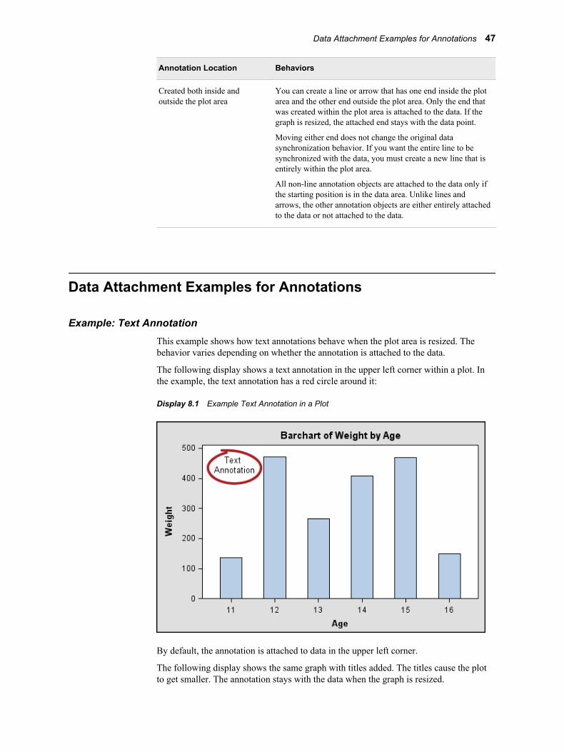
The following display shows a text annotation in the upper left corner within a plot. Inthe example, the text annotation has a red circle around it:
Display 8.1 Example Text Annotation in a Plot
By default, the annotation is attached to data in the upper left corner.
The following display shows the same graph with titles added. The titles cause the plotto get smaller. The annotation stays with the data when the graph is resized.
Data Attachment Examples for Annotations 47
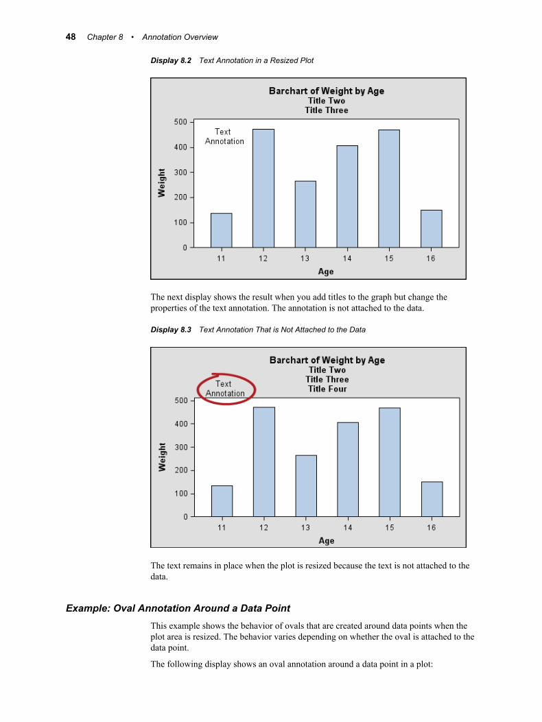
Display 8.2 Text Annotation in a Resized Plot
The next display shows the result when you add titles to the graph but change theproperties of the text annotation. The annotation is not attached to the data.
Display 8.3 Text Annotation That is Not Attached to the Data
The text remains in place when the plot is resized because the text is not attached to thedata.
Example: Oval Annotation Around a Data PointThis example shows the behavior of ovals that are created around data points when theplot area is resized. The behavior varies depending on whether the oval is attached to thedata point.
The following display shows an oval annotation around a data point in a plot:
48 Chapter 8 • Annotation Overview
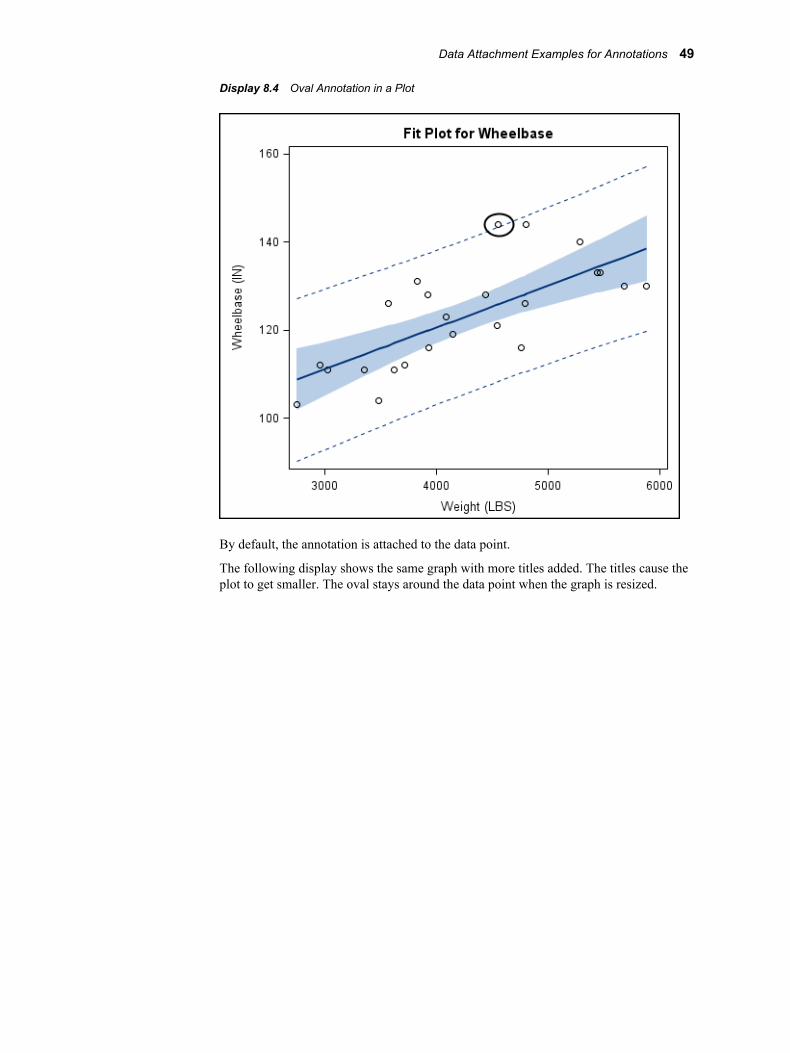
Display 8.4 Oval Annotation in a Plot
By default, the annotation is attached to the data point.
The following display shows the same graph with more titles added. The titles cause theplot to get smaller. The oval stays around the data point when the graph is resized.
Data Attachment Examples for Annotations 49
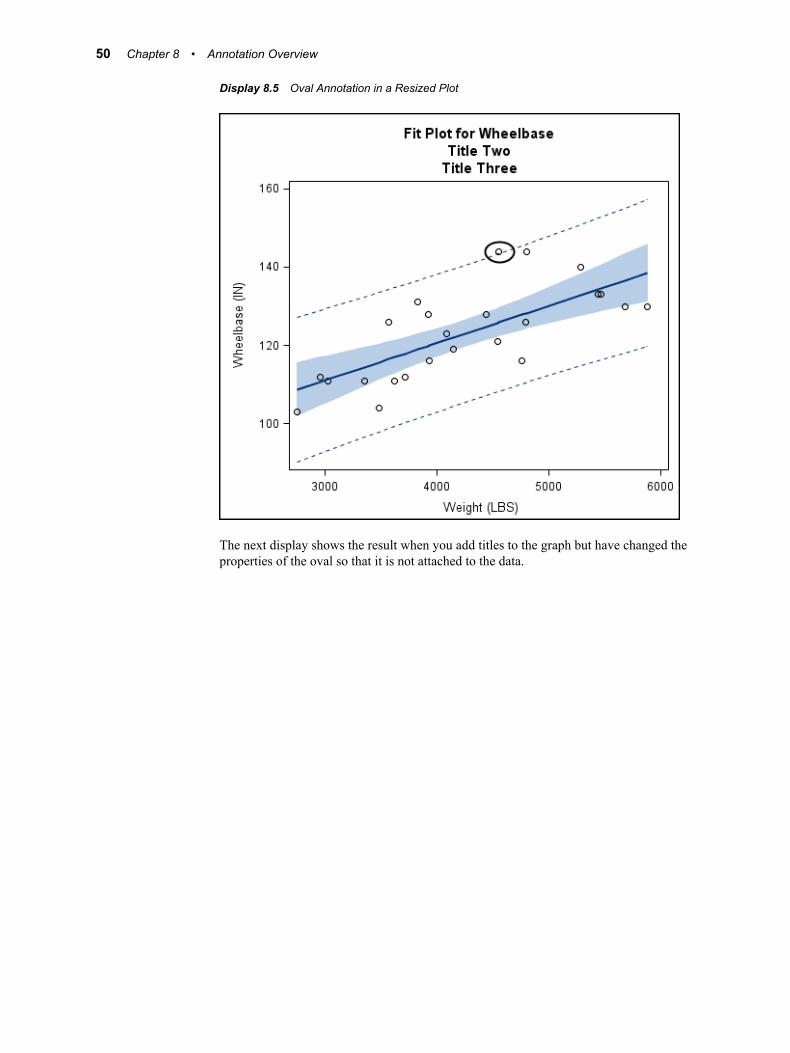
Display 8.5 Oval Annotation in a Resized Plot
The next display shows the result when you add titles to the graph but have changed theproperties of the oval so that it is not attached to the data.
50 Chapter 8 • Annotation Overview
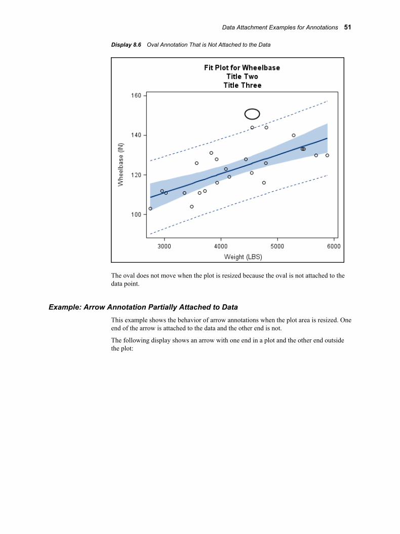
Display 8.6 Oval Annotation That is Not Attached to the Data
The oval does not move when the plot is resized because the oval is not attached to thedata point.
Example: Arrow Annotation Partially Attached to DataThis example shows the behavior of arrow annotations when the plot area is resized. Oneend of the arrow is attached to the data and the other end is not.
The following display shows an arrow with one end in a plot and the other end outsidethe plot:
Data Attachment Examples for Annotations 51
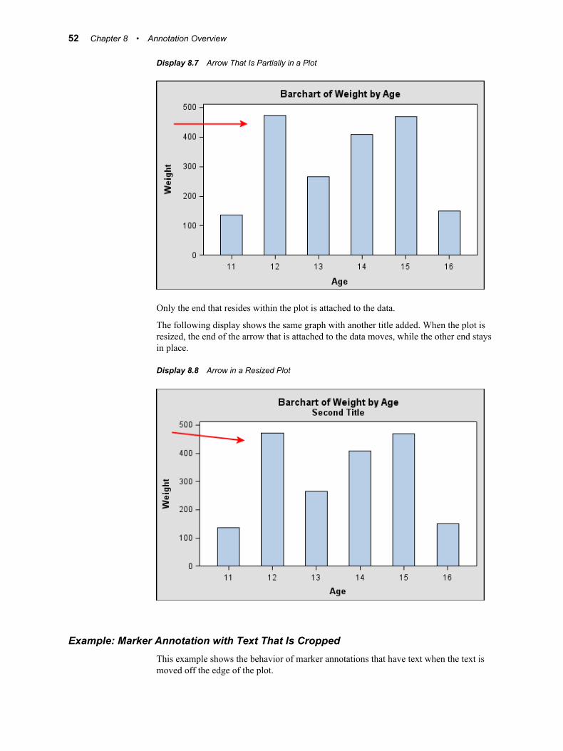
Display 8.7 Arrow That Is Partially in a Plot
Only the end that resides within the plot is attached to the data.
The following display shows the same graph with another title added. When the plot isresized, the end of the arrow that is attached to the data moves, while the other end staysin place.
Display 8.8 Arrow in a Resized Plot
Example: Marker Annotation with Text That Is CroppedThis example shows the behavior of marker annotations that have text when the text ismoved off the edge of the plot.
52 Chapter 8 • Annotation Overview
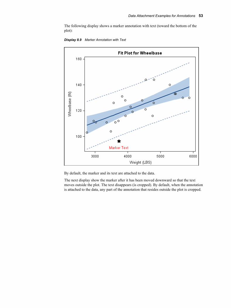
The following display shows a marker annotation with text (toward the bottom of theplot):
Display 8.9 Marker Annotation with Text
By default, the marker and its text are attached to the data.
The next display show the marker after it has been moved downward so that the textmoves outside the plot. The text disappears (is cropped). By default, when the annotationis attached to the data, any part of the annotation that resides outside the plot is cropped.
Data Attachment Examples for Annotations 53
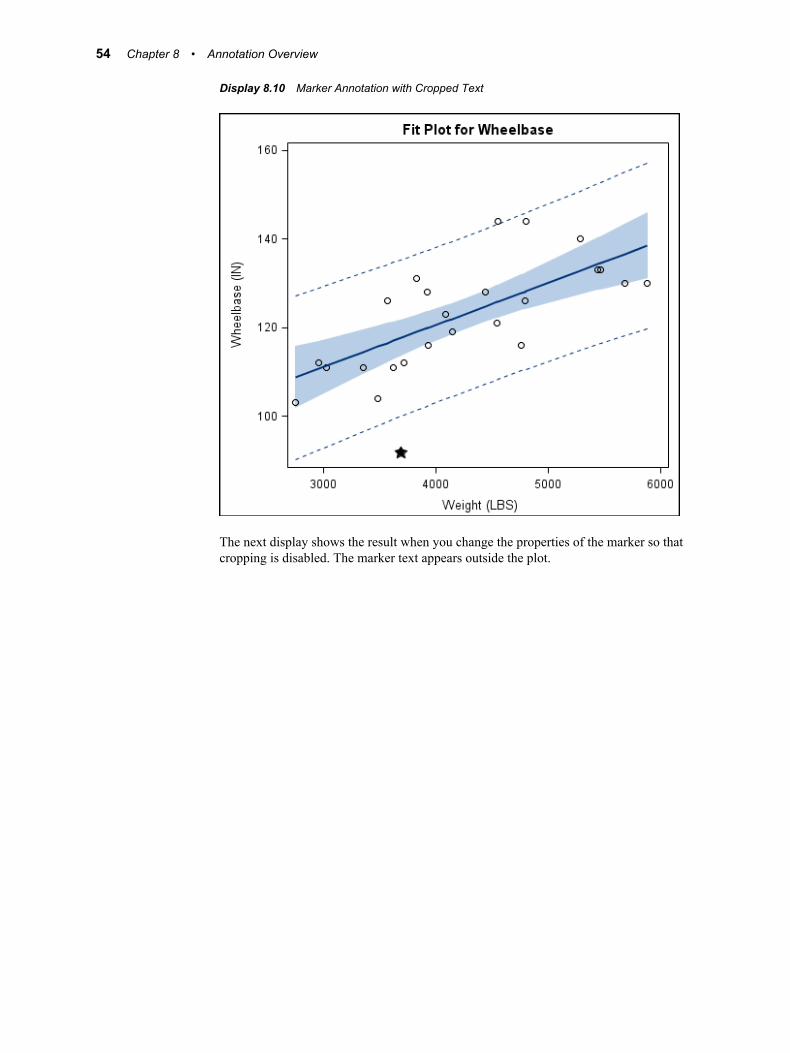
Display 8.10 Marker Annotation with Cropped Text
The next display shows the result when you change the properties of the marker so thatcropping is disabled. The marker text appears outside the plot.
54 Chapter 8 • Annotation Overview
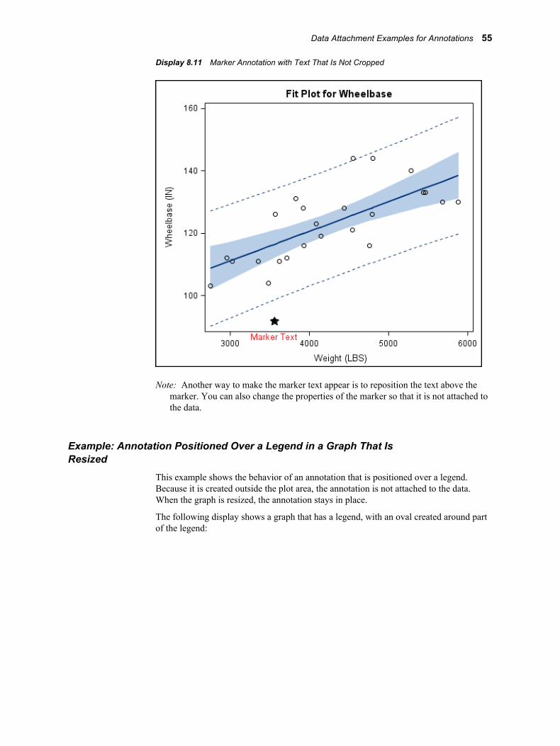
Display 8.11 Marker Annotation with Text That Is Not Cropped
Note: Another way to make the marker text appear is to reposition the text above themarker. You can also change the properties of the marker so that it is not attached tothe data.
Example: Annotation Positioned Over a Legend in a Graph That IsResized
This example shows the behavior of an annotation that is positioned over a legend.Because it is created outside the plot area, the annotation is not attached to the data.When the graph is resized, the annotation stays in place.
The following display shows a graph that has a legend, with an oval created around partof the legend:
Data Attachment Examples for Annotations 55
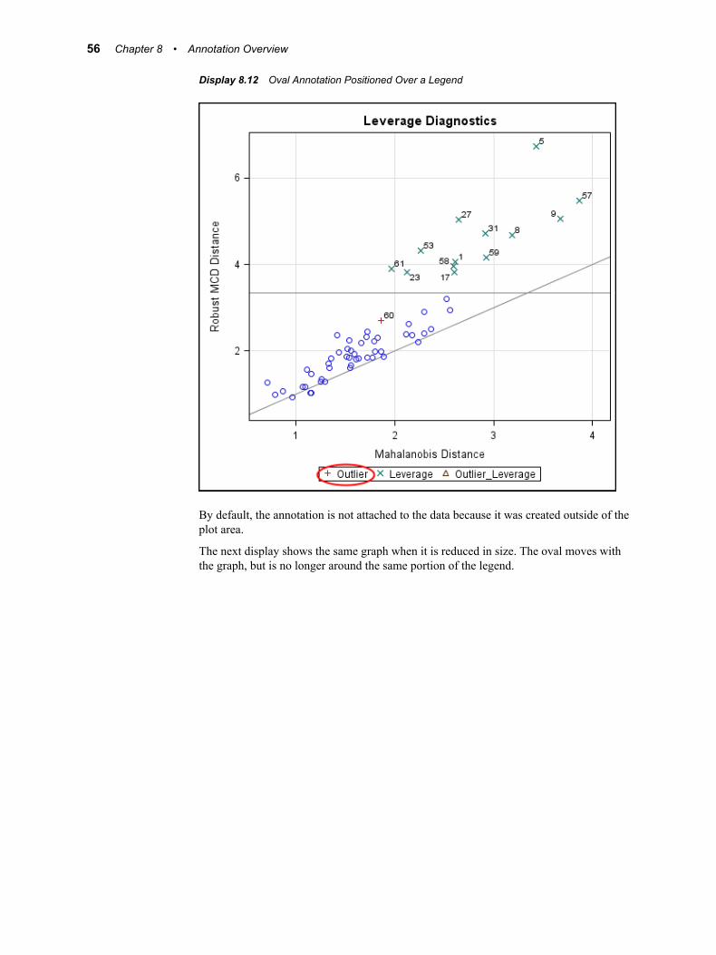
Display 8.12 Oval Annotation Positioned Over a Legend
By default, the annotation is not attached to the data because it was created outside of theplot area.
The next display shows the same graph when it is reduced in size. The oval moves withthe graph, but is no longer around the same portion of the legend.
56 Chapter 8 • Annotation Overview
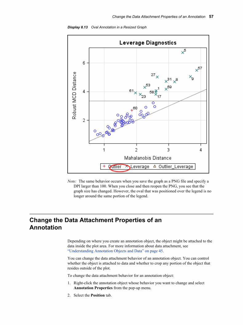
Display 8.13 Oval Annotation in a Resized Graph
Note: The same behavior occurs when you save the graph as a PNG file and specify aDPI larger than 100. When you close and then reopen the PNG, you see that thegraph size has changed. However, the oval that was positioned over the legend is nolonger around the same portion of the legend.
Change the Data Attachment Properties of anAnnotation
Depending on where you create an annotation object, the object might be attached to thedata inside the plot area. For more information about data attachment, see“Understanding Annotation Objects and Data” on page 45.
You can change the data attachment behavior of an annotation object. You can controlwhether the object is attached to data and whether to crop any portion of the object thatresides outside of the plot.
To change the data attachment behavior for an annotation object:
1. Right-click the annotation object whose behavior you want to change and selectAnnotation Properties from the pop-up menu.
2. Select the Position tab.
Change the Data Attachment Properties of an Annotation 57
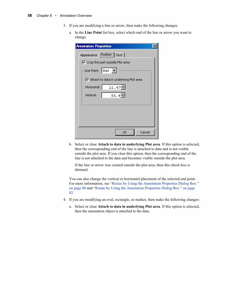
3. If you are modifying a line or arrow, then make the following changes:
a. In the Line Point list box, select which end of the line or arrow you want tochange.
b. Select or clear Attach to data in underlying Plot area. If this option is selected,then the corresponding end of the line is attached to data and is not visibleoutside the plot area. If you clear this option, then the corresponding end of theline is not attached to the data and becomes visible outside the plot area.
If the line or arrow was created outside the plot area, then this check box isdimmed.
You can also change the vertical or horizontal placement of the selected end point.For more information, see “Resize by Using the Annotation Properties Dialog Box ”on page 80 and “Rotate by Using the Annotation Properties Dialog Box ” on page82.
4. If you are modifying an oval, rectangle, or marker, then make the following changes:
a. Select or clear Attach to data in underlying Plot area. If this option is selected,then the annotation object is attached to the data.
58 Chapter 8 • Annotation Overview
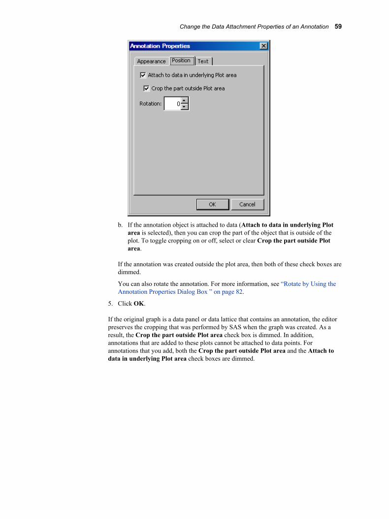
b. If the annotation object is attached to data (Attach to data in underlying Plotarea is selected), then you can crop the part of the object that is outside of theplot. To toggle cropping on or off, select or clear Crop the part outside Plotarea.
If the annotation was created outside the plot area, then both of these check boxes aredimmed.
You can also rotate the annotation. For more information, see “Rotate by Using theAnnotation Properties Dialog Box ” on page 82.
5. Click OK.
If the original graph is a data panel or data lattice that contains an annotation, the editorpreserves the cropping that was performed by SAS when the graph was created. As aresult, the Crop the part outside Plot area check box is dimmed. In addition,annotations that are added to these plots cannot be attached to data points. Forannotations that you add, both the Crop the part outside Plot area and the Attach todata in underlying Plot area check boxes are dimmed.
Change the Data Attachment Properties of an Annotation 59

60 Chapter 8 • Annotation Overview
Chapter 9
Using Annotations in a Graph
About Text Annotations . . . . . . . . . . . . . . . . . . . . . . . . . . . . . . . . . . . . . . . . . . . . . . . . 61
Add a Text Annotation to a Graph . . . . . . . . . . . . . . . . . . . . . . . . . . . . . . . . . . . . . . . 62
Edit a Text Annotation . . . . . . . . . . . . . . . . . . . . . . . . . . . . . . . . . . . . . . . . . . . . . . . . . 62
About Lines and Arrows . . . . . . . . . . . . . . . . . . . . . . . . . . . . . . . . . . . . . . . . . . . . . . . 62
Add a Line to a Graph . . . . . . . . . . . . . . . . . . . . . . . . . . . . . . . . . . . . . . . . . . . . . . . . . 63
Add an Arrow to a Graph . . . . . . . . . . . . . . . . . . . . . . . . . . . . . . . . . . . . . . . . . . . . . . 63
About Ovals and Rectangles . . . . . . . . . . . . . . . . . . . . . . . . . . . . . . . . . . . . . . . . . . . . 64
Add an Oval to a Graph . . . . . . . . . . . . . . . . . . . . . . . . . . . . . . . . . . . . . . . . . . . . . . . . 65
Add a Rectangle to a Graph . . . . . . . . . . . . . . . . . . . . . . . . . . . . . . . . . . . . . . . . . . . . 65
About Markers . . . . . . . . . . . . . . . . . . . . . . . . . . . . . . . . . . . . . . . . . . . . . . . . . . . . . . . 65
Add a Marker to a Graph . . . . . . . . . . . . . . . . . . . . . . . . . . . . . . . . . . . . . . . . . . . . . . 66
About Images . . . . . . . . . . . . . . . . . . . . . . . . . . . . . . . . . . . . . . . . . . . . . . . . . . . . . . . . 66
Add and Position an Image in a Graph . . . . . . . . . . . . . . . . . . . . . . . . . . . . . . . . . . . 67
About Text Annotations
You can change the appearance of a graph by adding text annotations. For instructionson working with text annotations, see the following topics:
• “Add a Text Annotation to a Graph” on page 62
• “Edit a Text Annotation” on page 62
• “Format a Text Annotation” on page 69
You can also make the following changes:
• Change the size of a text annotation. For instructions, see “Resize an Annotation” onpage 79.
• Rotate a text annotation. For instructions, see “Rotate an Annotation” on page 81.
• Move a text annotation. For instructions, see “Move an Annotation” on page 83.
• Change the data attachment properties of a text annotation. For instructions, see“Change the Data Attachment Properties of an Annotation” on page 57.
61
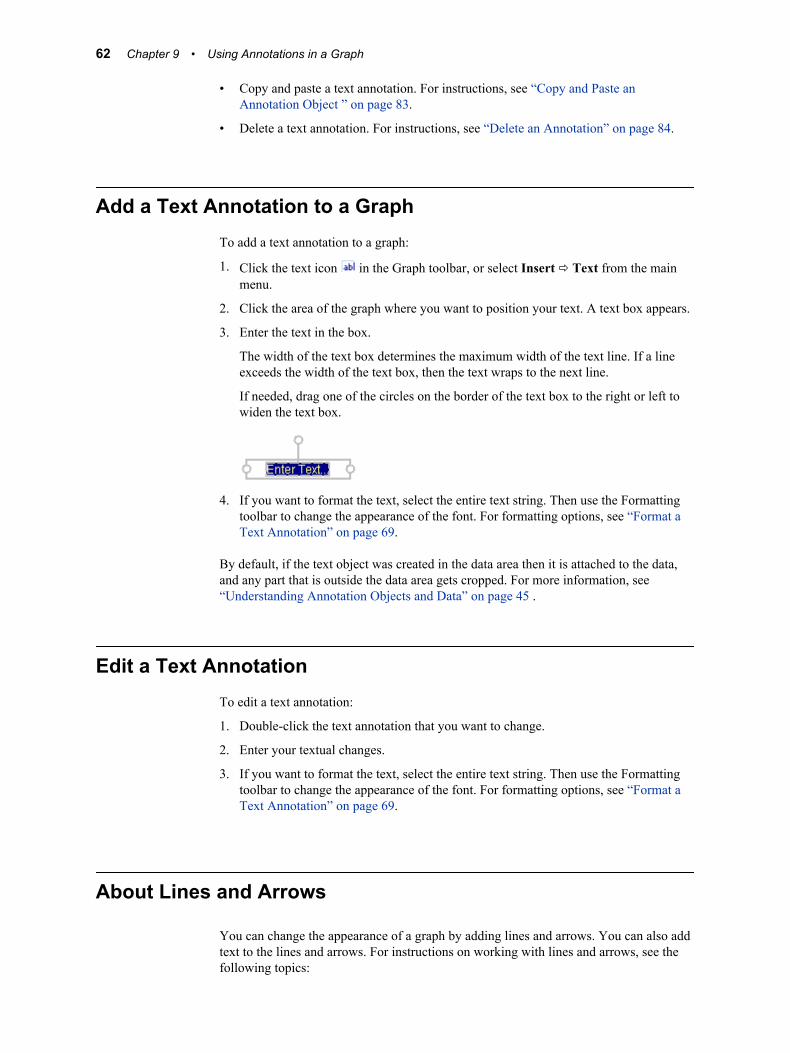
• Copy and paste a text annotation. For instructions, see “Copy and Paste anAnnotation Object ” on page 83.
• Delete a text annotation. For instructions, see “Delete an Annotation” on page 84.
Add a Text Annotation to a GraphTo add a text annotation to a graph:
1. Click the text icon in the Graph toolbar, or select Insert ð Text from the mainmenu.
2. Click the area of the graph where you want to position your text. A text box appears.
3. Enter the text in the box.
The width of the text box determines the maximum width of the text line. If a lineexceeds the width of the text box, then the text wraps to the next line.
If needed, drag one of the circles on the border of the text box to the right or left towiden the text box.
4. If you want to format the text, select the entire text string. Then use the Formattingtoolbar to change the appearance of the font. For formatting options, see “Format aText Annotation” on page 69.
By default, if the text object was created in the data area then it is attached to the data,and any part that is outside the data area gets cropped. For more information, see “Understanding Annotation Objects and Data” on page 45 .
Edit a Text AnnotationTo edit a text annotation:
1. Double-click the text annotation that you want to change.
2. Enter your textual changes.
3. If you want to format the text, select the entire text string. Then use the Formattingtoolbar to change the appearance of the font. For formatting options, see “Format aText Annotation” on page 69.
About Lines and Arrows
You can change the appearance of a graph by adding lines and arrows. You can also addtext to the lines and arrows. For instructions on working with lines and arrows, see thefollowing topics:
62 Chapter 9 • Using Annotations in a Graph
• “Add a Line to a Graph” on page 63
• “Add an Arrow to a Graph” on page 63
• “Change the Color, Pattern, and Thickness of a Line or Arrow” on page 69
You can also make the following changes:
• Add text to a line or arrow. For instructions, see “Add Text to an Annotation” onpage 75.
• Change the length of a line or arrow. For instructions, see “Resize an Annotation” onpage 79.
• Rotate a line or arrow. For instructions, see “Rotate an Annotation” on page 81.
• Move a line or arrow. For instructions, see “Move an Annotation” on page 83.
• Change the data attachment properties of a line or arrow. For instructions, see“Change the Data Attachment Properties of an Annotation” on page 57.
• Copy and paste a line or arrow. For instructions, see “Copy and Paste an AnnotationObject ” on page 83.
• Delete a line or arrow. For instructions, see “Delete an Annotation” on page 84.
Add a Line to a GraphTo add a line to a graph:
1. Click the line icon in the Graph toolbar, or select Insert ð Line from the mainmenu.
2. Position your cursor at a starting position in the graph.
3. Click and drag to create the line in the graph.
You can control the line as follows:
• If you press the CTRL key and then click and drag, the line is created from thecenter and moves outward.
• If you press SHIFT and then click and drag, then the line's orientation stays inmultiples of 15 degrees. You can create a perfect horizontal or vertical line thisway. You can also rotate the line in 15 degree increments to create a diagonalline.
• If you press CTRL+SHIFT and then click and drag, the line is created from thecenter, moves outward, and can be rotated in 15 degree increments.
You can add text to the line. For instructions, see “Add Text to an Annotation” on page75.
Add an Arrow to a GraphYou can add an arrow to a graph to point out specific information. To add an arrow to agraph:
Add an Arrow to a Graph 63
1. Click the arrow icon in the Graph toolbar, or select Insert ð Arrow from themain menu.
2. Position your cursor at a starting position in the graph.
3. Click and drag to create the arrow. By default, the arrow is drawn from the tail to thehead.
You can control the arrow as follows:
• If you press the CTRL key and then click and drag, the arrow is created from thehead to the tail.
• If you press SHIFT and then click and drag, then the arrow's orientation stays inmultiples of 15 degrees. You can create a perfect horizontal or vertical arrow thisway. You can also rotate the arrow in 15 degree increments to create a diagonalarrow.
• If you press CTRL+SHIFT and then click and drag, the arrow is created from thehead to the tail, and can be positioned in 15 degree increments.
After you create the arrow, you can add text to the tail end of the arrow. For instructions,see “Add Text to an Annotation” on page 75.
About Ovals and Rectangles
You can change the appearance of a graph by adding ovals (or circles) and rectangles (orsquares). You can also add text to the ovals and rectangles. For instructions on workingwith ovals and rectangles, see the following topics:
• “Add an Oval to a Graph” on page 65
• “Add a Rectangle to a Graph” on page 65
• “Change the Color, Transparency, and Outline Properties of an Oval or Rectangle”on page 70
You can also make the following changes:
• Add text to an oval or rectangle. For instructions, see “Add Text to an Annotation”on page 75.
• Change the size of an oval or rectangle. For instructions, see “Resize an Annotation”on page 79.
• Rotate an oval or rectangle. For instructions, see “Rotate an Annotation” on page81.
• Move an oval or rectangle. For instructions, see “Move an Annotation” on page 83.
• Change the data attachment properties of an oval or rectangle. For instructions, see“Change the Data Attachment Properties of an Annotation” on page 57.
• Copy and paste an oval or rectangle. For instructions, see “Copy and Paste anAnnotation Object ” on page 83.
• Delete an oval or rectangle. For instructions, see “Delete an Annotation” on page84.
64 Chapter 9 • Using Annotations in a Graph
Add an Oval to a Graph
To add an oval (or a circle) to a graph:
1. Click the oval icon in the Graph toolbar, or select Insert ð Oval from the menu.
2. Place your cursor at the top left position in the graph where you want your oval tobegin.
3. Click and drag your cursor to the right to create an oval.
You can control the oval as follows:
• If you press the CTRL key and then click and drag, the oval expands from thecenter.
• If you press the SHIFT key and then click and drag, you can draw a perfectcircle.
• If you press SHIFT + CTRL and then click and drag, you draw a circle thatexpands from the center.
You can add text to the oval. For instructions, see “Add Text to an Annotation” on page75.
Add a Rectangle to a GraphTo add a rectangle (or a square) to a graph:
1. Click the rectangle icon in the Graph toolbar, or select Insert ð Rectangle fromthe menu.
2. Place your cursor at the top left position in the graph where you want your rectangleto begin.
3. Click and drag your cursor to the right to create a rectangle.
You can control the rectangle as follows:
• If you press the CTRL key and then click and drag, the rectangle expands fromthe center.
• If you press the SHIFT key and then click and drag, you can draw a perfectsquare.
• If you press SHIFT + CTRL and then click and drag, you draw a square thatexpands from the center.
You can add text to the rectangle or square. For instructions, see “Add Text to anAnnotation” on page 75.
About Markers
About Markers 65
You can change the appearance of a graph by adding markers to the graph. Forinstructions on working with markers, see the following topics:
• “Add a Marker to a Graph” on page 66
• “Change the Color, Symbol, and Size of a Marker” on page 71
You can also make the following changes:
• Add text to a marker. For instructions, see “Add Text to an Annotation” on page75.
• Rotate a marker. For instructions, see “Rotate an Annotation” on page 81.
• Move a marker. For instructions, see “Move an Annotation” on page 83.
• Change the data attachment properties of a marker. For instructions, see “Change theData Attachment Properties of an Annotation” on page 57.
• Copy and paste a marker. For instructions, see “Copy and Paste an AnnotationObject ” on page 83.
• Delete a marker. For instructions, see “Delete an Annotation” on page 84.
Add a Marker to a GraphYou can use a marker to identify or accentuate key data elements in a graph, such as datapoints that are outliers.
To add a marker to a graph:
1.Click the marker icon in the Graph toolbar, or select Insert ð Marker from themain menu.
Note: As shown here, the marker icon is a star. The icon in your operatingenvironment might be different. In addition, you can change the symbol that isused for the icon. For instructions, see “Change the Color, Symbol, and Size of aMarker” on page 71.
2. Click the area of the graph where you want to place the marker.
You can add text to the marker. For instructions, see “Add Text to an Annotation” onpage 75.
About Images
You can add images to a graph. For instructions on working with images, see thefollowing topics:
• “Add and Position an Image in a Graph” on page 67
• “Format an Outline Around an Image” on page 72
You can also make the following changes:
• Add text to an image. For instructions, see “Add Text to an Annotation” on page75.
66 Chapter 9 • Using Annotations in a Graph
• Change the size of an image. For instructions, see “Resize an Annotation” on page79.
• Rotate an image. For instructions, see “Rotate an Annotation” on page 81.
• Move an image. For instructions, see “Move an Annotation” on page 83.
• Copy and paste an image. For instructions, see “Copy and Paste an AnnotationObject ” on page 83.
• Delete an image from a graph. For instructions, see “Delete an Annotation” on page84.
Add and Position an Image in a GraphYou can add an image, such as a logo, to a graph. When you add an image to a graph,the image appears in the center of the graph. You can reposition and resize the image ifnecessary.
To add, resize, and reposition an image:
1. Click from the Graph toolbar, or select Insert ð Image from the main menu.
2. From the Image dialog box that displays, select and open the image that you want toinsert.
The image appears in the center of the graph.
3. To resize the image, select the image and drag one of the circles that appear aroundthe image. You can maintain the ratio of width to length. Position your cursor on acorner circle, press SHIFT, and drag the corner circle.
4. To move the image to a different position, click and drag the image to anotherposition in the graph.
Note: Images are not attached to the data. For more information about data attachment,see “Understanding Annotation Objects and Data” on page 45.
Add and Position an Image in a Graph 67

68 Chapter 9 • Using Annotations in a Graph
Chapter 10
Changing the Visual Properties ofAnnotations
Format a Text Annotation . . . . . . . . . . . . . . . . . . . . . . . . . . . . . . . . . . . . . . . . . . . . . . 69
Change the Color, Pattern, and Thickness of a Line or Arrow . . . . . . . . . . . . . . . . 69
Change the Color, Transparency, and Outline Properties ofan Oval or Rectangle . . . . . . . . . . . . . . . . . . . . . . . . . . . . . . . . . . . . . . . . . . . . . . . . . . 70
Change the Color, Symbol, and Size of a Marker . . . . . . . . . . . . . . . . . . . . . . . . . . . 71
Format an Outline Around an Image . . . . . . . . . . . . . . . . . . . . . . . . . . . . . . . . . . . . . 72
Format a Text AnnotationYou can change the font, size, style (for example, bold or italicized), alignment, or colorof the text in a text annotation.
To format a text annotation:
1. Click the text annotation.
2. Use the Formatting toolbar to make your changes. For details, see “Using theFormatting Toolbar” on page 21.
Text format changes that you make here remain in effect for new annotations that youadd.
As an alternative to this procedure, you can right-click the text annotation, selectAnnotation Properties, and make your changes in the Text tab. You can change thefont, size, style, and color.
Change the Color, Pattern, and Thickness of aLine or Arrow
To change the color, pattern (such as dotted or dashed), or thickness of a line or arrow:
1. Right-click the line or arrow and select Annotation Properties from the menu. TheAnnotation Properties dialog box appears.
69
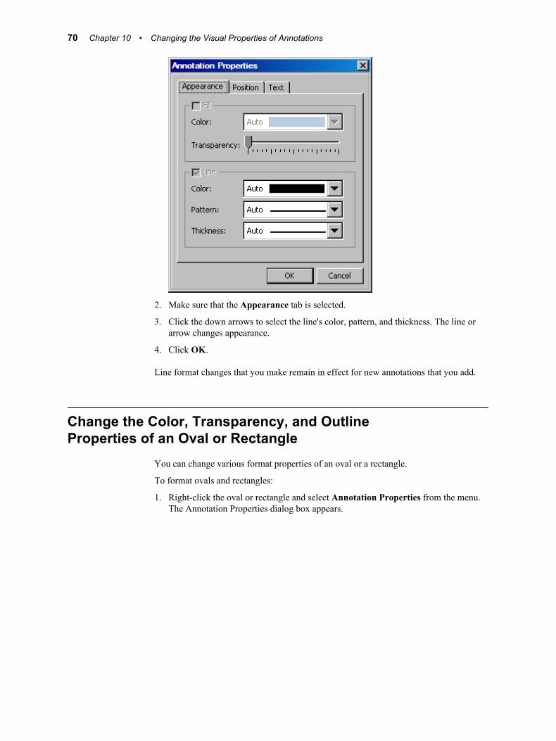
2. Make sure that the Appearance tab is selected.
3. Click the down arrows to select the line's color, pattern, and thickness. The line orarrow changes appearance.
4. Click OK.
Line format changes that you make remain in effect for new annotations that you add.
Change the Color, Transparency, and OutlineProperties of an Oval or Rectangle
You can change various format properties of an oval or a rectangle.
To format ovals and rectangles:
1. Right-click the oval or rectangle and select Annotation Properties from the menu.The Annotation Properties dialog box appears.
70 Chapter 10 • Changing the Visual Properties of Annotations
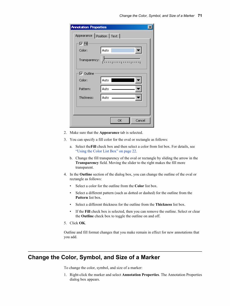
2. Make sure that the Appearance tab is selected.
3. You can specify a fill color for the oval or rectangle as follows:
a. Select theFill check box and then select a color from list box. For details, see“Using the Color List Box” on page 22.
b. Change the fill transparency of the oval or rectangle by sliding the arrow in theTransparency field. Moving the slider to the right makes the fill moretransparent.
4. In the Outline section of the dialog box, you can change the outline of the oval orrectangle as follows:
• Select a color for the outline from the Color list box.
• Select a different pattern (such as dotted or dashed) for the outline from thePattern list box.
• Select a different thickness for the outline from the Thickness list box.
• If the Fill check box is selected, then you can remove the outline. Select or clearthe Outline check box to toggle the outline on and off.
5. Click OK.
Outline and fill format changes that you make remain in effect for new annotations thatyou add.
Change the Color, Symbol, and Size of a MarkerTo change the color, symbol, and size of a marker:
1. Right-click the marker and select Annotation Properties. The Annotation Propertiesdialog box appears.
Change the Color, Symbol, and Size of a Marker 71
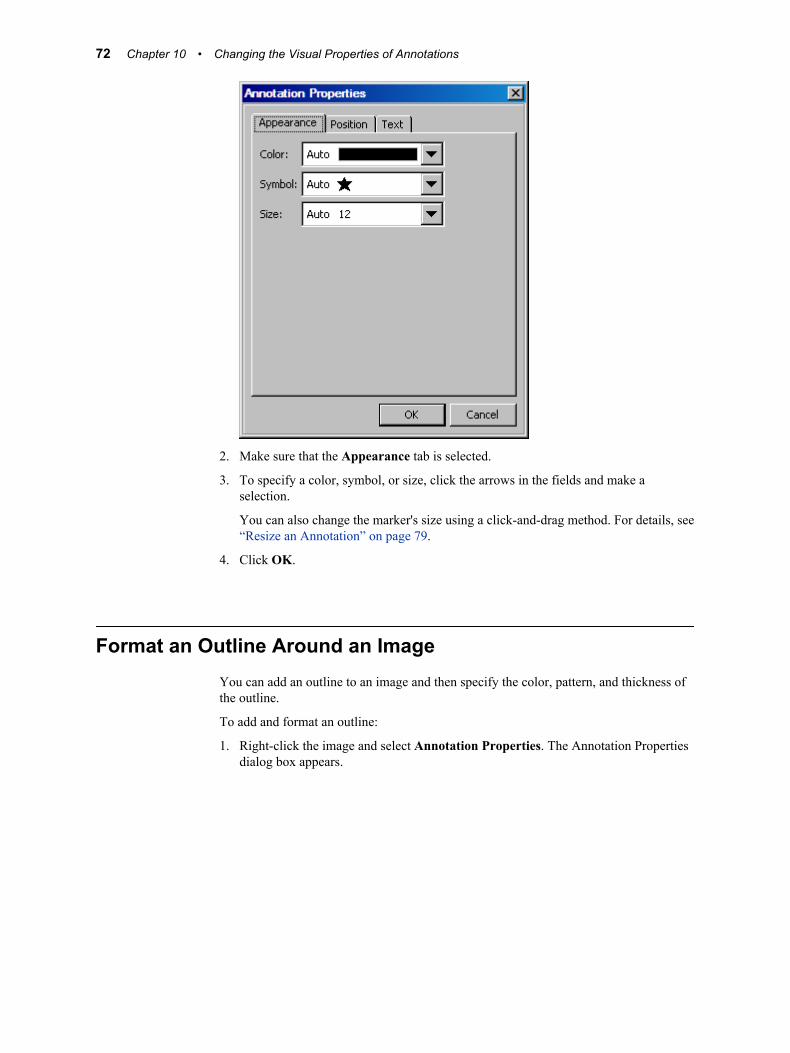
2. Make sure that the Appearance tab is selected.
3. To specify a color, symbol, or size, click the arrows in the fields and make aselection.
You can also change the marker's size using a click-and-drag method. For details, see“Resize an Annotation” on page 79.
4. Click OK.
Format an Outline Around an ImageYou can add an outline to an image and then specify the color, pattern, and thickness ofthe outline.
To add and format an outline:
1. Right-click the image and select Annotation Properties. The Annotation Propertiesdialog box appears.
72 Chapter 10 • Changing the Visual Properties of Annotations
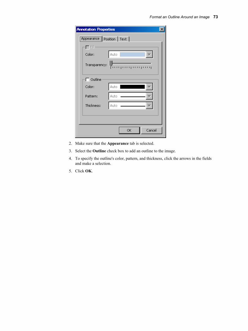
2. Make sure that the Appearance tab is selected.
3. Select the Outline check box to add an outline to the image.
4. To specify the outline's color, pattern, and thickness, click the arrows in the fieldsand make a selection.
5. Click OK.
Format an Outline Around an Image 73

74 Chapter 10 • Changing the Visual Properties of Annotations
Chapter 11
Adding Text to Annotations
Overview of Adding Text to Annotations . . . . . . . . . . . . . . . . . . . . . . . . . . . . . . . . . . 75
Add Text to an Annotation . . . . . . . . . . . . . . . . . . . . . . . . . . . . . . . . . . . . . . . . . . . . . 75
Edit Text That Has Been Added to an Annotation . . . . . . . . . . . . . . . . . . . . . . . . . . 76
Format Text That Has Been Added to an Annotation . . . . . . . . . . . . . . . . . . . . . . . 76
Move Text That Has Been Added to an Annotation . . . . . . . . . . . . . . . . . . . . . . . . . 77
Overview of Adding Text to Annotations
In addition to adding text annotations to a graph, you can add text to lines, arrows, ovals,rectangles, images, and markers.
Note: When you create an arrow in your graph, a text box appears. The text boxdisappears if you click outside the arrow without entering text. You can later add textto the arrow.
For instructions on working with annotations and text, see the following topics:
• “Add Text to an Annotation” on page 75
• “Edit Text That Has Been Added to an Annotation” on page 76
• “Format Text That Has Been Added to an Annotation” on page 76
• “Move Text That Has Been Added to an Annotation” on page 77
Add Text to an AnnotationTo add text to an annotation:
1. Right-click the annotation object and select Add ('Edit') Text from the pop-upmenu.
A text box appears. The location of the text box depends on the type of annotation.
• For ovals and rectangles, the text box appears inside the oval or rectangle.
75
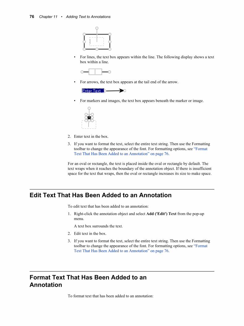
• For lines, the text box appears within the line. The following display shows a textbox within a line.
• For arrows, the text box appears at the tail end of the arrow.
• For markers and images, the text box appears beneath the marker or image.
2. Enter text in the box.
3. If you want to format the text, select the entire text string. Then use the Formattingtoolbar to change the appearance of the font. For formatting options, see “FormatText That Has Been Added to an Annotation” on page 76.
For an oval or rectangle, the text is placed inside the oval or rectangle by default. Thetext wraps when it reaches the boundary of the annotation object. If there is insufficientspace for the text that wraps, then the oval or rectangle increases its size to make space.
Edit Text That Has Been Added to an AnnotationTo edit text that has been added to an annotation:
1. Right-click the annotation object and select Add ('Edit') Text from the pop-upmenu.
A text box surrounds the text.
2. Edit text in the box.
3. If you want to format the text, select the entire text string. Then use the Formattingtoolbar to change the appearance of the font. For formatting options, see “FormatText That Has Been Added to an Annotation” on page 76.
Format Text That Has Been Added to anAnnotation
To format text that has been added to an annotation:
76 Chapter 11 • Adding Text to Annotations
1. Right-click the annotation object and select Add ('Edit') Text from the pop-upmenu.
A text box surrounds the text.
2. Select the entire text string. Then use the Formatting toolbar to change theappearance of the font. For details, see “Using the Formatting Toolbar” on page 21.
Changes that you make remain in effect for any new annotations that you add.
As an alternative to this procedure, you can right-click the text annotation, selectAnnotation Properties, and make your changes in the Text tab. You can change thefont, size, style (for example, bold or italicized), and color.
Move Text That Has Been Added to an AnnotationTo move text that has been added to an annotation:
1. Right-click the annotation object and select Annotation Properties from the pop-upmenu.
2. Select the Text tab.
3. Select the desired position for the text as follows:
• For lines and arrows, select the Through, Above, Below, Start, or End radiobutton to position the text with respect to the line or arrow.
• For all other annotation objects, select the Inside, Above, or Below radio buttonto position the text with respect to the object.
4. Click OK.
For all annotations other than images, if your selection places the text outside of the plot,then the text might be cropped. For more information, see “Understanding AnnotationObjects and Data” on page 45. To turn cropping off, see “Change the Data AttachmentProperties of an Annotation” on page 57.
Move Text That Has Been Added to an Annotation 77

78 Chapter 11 • Adding Text to Annotations
Chapter 12
Modifying Annotations
Resize an Annotation . . . . . . . . . . . . . . . . . . . . . . . . . . . . . . . . . . . . . . . . . . . . . . . . . . 79Resize by Dragging . . . . . . . . . . . . . . . . . . . . . . . . . . . . . . . . . . . . . . . . . . . . . . . . . . 79Resize by Using the Annotation Properties Dialog Box . . . . . . . . . . . . . . . . . . . . . 80
Rotate an Annotation . . . . . . . . . . . . . . . . . . . . . . . . . . . . . . . . . . . . . . . . . . . . . . . . . . 81Rotate by Dragging the Annotation . . . . . . . . . . . . . . . . . . . . . . . . . . . . . . . . . . . . . 81Rotate by Using the Annotation Properties Dialog Box . . . . . . . . . . . . . . . . . . . . . . 82
Move an Annotation . . . . . . . . . . . . . . . . . . . . . . . . . . . . . . . . . . . . . . . . . . . . . . . . . . . 83
Copy and Paste an Annotation Object . . . . . . . . . . . . . . . . . . . . . . . . . . . . . . . . . . . . 83
Delete an Annotation . . . . . . . . . . . . . . . . . . . . . . . . . . . . . . . . . . . . . . . . . . . . . . . . . . 84
Working with Groups of Annotation Objects . . . . . . . . . . . . . . . . . . . . . . . . . . . . . . 84
Change the Order of Annotation Objects . . . . . . . . . . . . . . . . . . . . . . . . . . . . . . . . . 84
Align Multiple Annotation Objects . . . . . . . . . . . . . . . . . . . . . . . . . . . . . . . . . . . . . . . 85
Resize an Annotation
Resize by DraggingTo change the size of an annotation:
1. Click the annotation object that you want to resize.
Small circles surround the object. If you click a line or arrow, a circle appears at eachend of the line or arrow.
2. Click and drag a circle to change the size of the annotation as follows:
• To change the length of a line or arrow, drag an end circle backward or forward.
Press SHIFT and drag to keep the line or arrow perfectly horizontal, vertical, ordiagonal in 15 degree increments.
• To resize all other annotations, drag one of the circles to expand or reduce theannotation. To change the width and length of the annotation simultaneously,position the cursor in a circle at one of the corners.
79
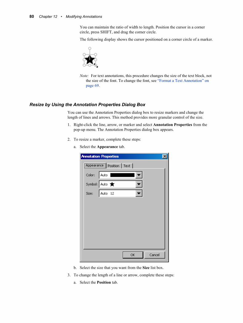
You can maintain the ratio of width to length. Position the cursor in a cornercircle, press SHIFT, and drag the corner circle.
The following display shows the cursor positioned on a corner circle of a marker.
Note: For text annotations, this procedure changes the size of the text block, notthe size of the font. To change the font, see “Format a Text Annotation” onpage 69.
Resize by Using the Annotation Properties Dialog BoxYou can use the Annotation Properties dialog box to resize markers and change thelength of lines and arrows. This method provides more granular control of the size.
1. Right-click the line, arrow, or marker and select Annotation Properties from thepop-up menu. The Annotation Properties dialog box appears.
2. To resize a marker, complete these steps:
a. Select the Appearance tab.
b. Select the size that you want from the Size list box.
3. To change the length of a line or arrow, complete these steps:
a. Select the Position tab.
80 Chapter 12 • Modifying Annotations
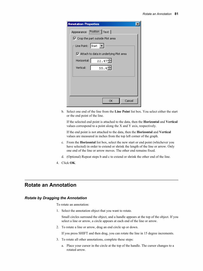
b. Select one end of the line from the Line Point list box. You select either the startor the end point of the line.
If the selected end point is attached to the data, then the Horizontal and Verticalvalues correspond to a point along the X and Y axis, respectively.
If the end point is not attached to the data, then the Horizontal and Verticalvalues are measured in inches from the top left corner of the graph.
c. From the Horizontal list box, select the new start or end point (whichever youhave selected) in order to extend or shrink the length of the line or arrow. Onlyone end of the line or arrow moves. The other end remains fixed.
d. (Optional) Repeat steps b and c to extend or shrink the other end of the line.
4. Click OK.
Rotate an Annotation
Rotate by Dragging the AnnotationTo rotate an annotation:
1. Select the annotation object that you want to rotate.
Small circles surround the object, and a handle appears at the top of the object. If youselect a line or arrow, a circle appears at each end of the line or arrow.
2. To rotate a line or arrow, drag an end circle up or down.
If you press SHIFT and then drag, you can rotate the line in 15 degree increments.
3. To rotate all other annotations, complete these steps:
a. Place your cursor in the circle at the top of the handle. The cursor changes to arotated arrow.
Rotate an Annotation 81
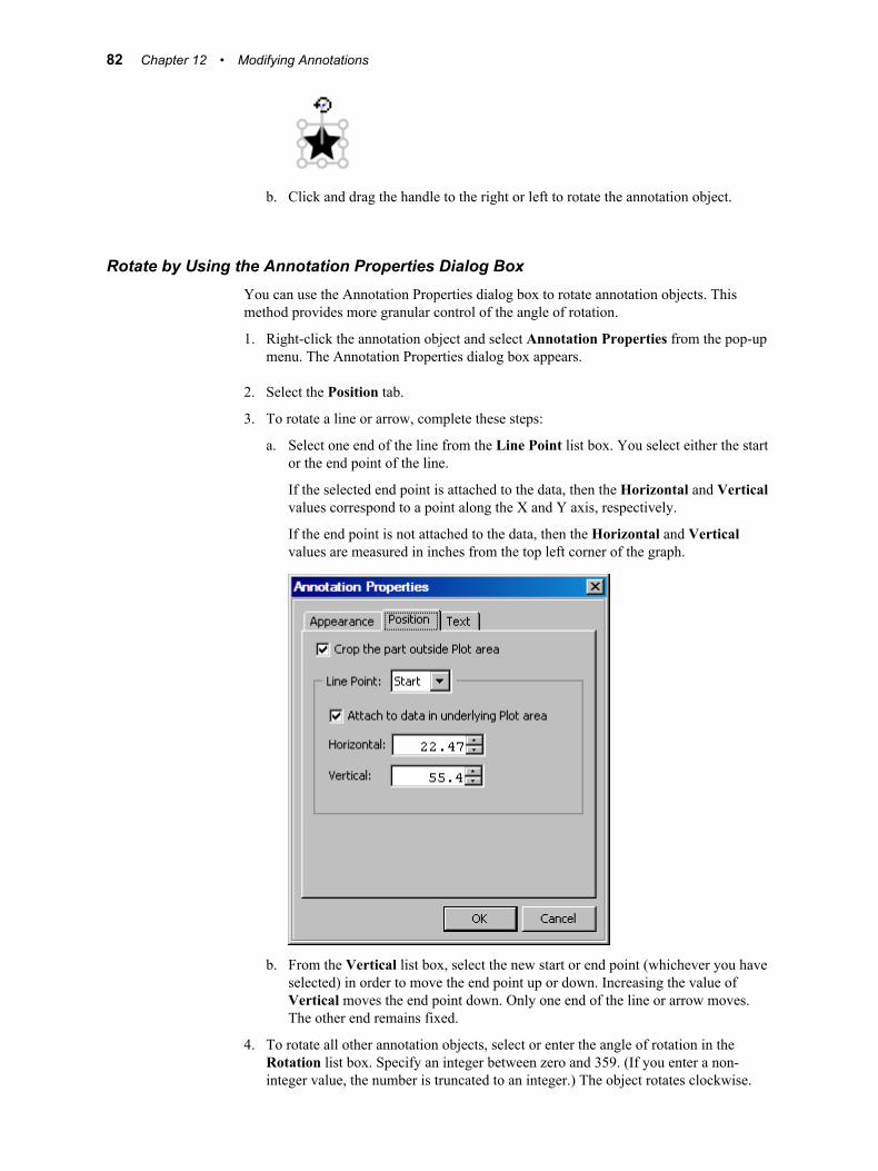
b. Click and drag the handle to the right or left to rotate the annotation object.
Rotate by Using the Annotation Properties Dialog BoxYou can use the Annotation Properties dialog box to rotate annotation objects. Thismethod provides more granular control of the angle of rotation.
1. Right-click the annotation object and select Annotation Properties from the pop-upmenu. The Annotation Properties dialog box appears.
2. Select the Position tab.
3. To rotate a line or arrow, complete these steps:
a. Select one end of the line from the Line Point list box. You select either the startor the end point of the line.
If the selected end point is attached to the data, then the Horizontal and Verticalvalues correspond to a point along the X and Y axis, respectively.
If the end point is not attached to the data, then the Horizontal and Verticalvalues are measured in inches from the top left corner of the graph.
b. From the Vertical list box, select the new start or end point (whichever you haveselected) in order to move the end point up or down. Increasing the value ofVertical moves the end point down. Only one end of the line or arrow moves.The other end remains fixed.
4. To rotate all other annotation objects, select or enter the angle of rotation in theRotation list box. Specify an integer between zero and 359. (If you enter a non-integer value, the number is truncated to an integer.) The object rotates clockwise.
82 Chapter 12 • Modifying Annotations
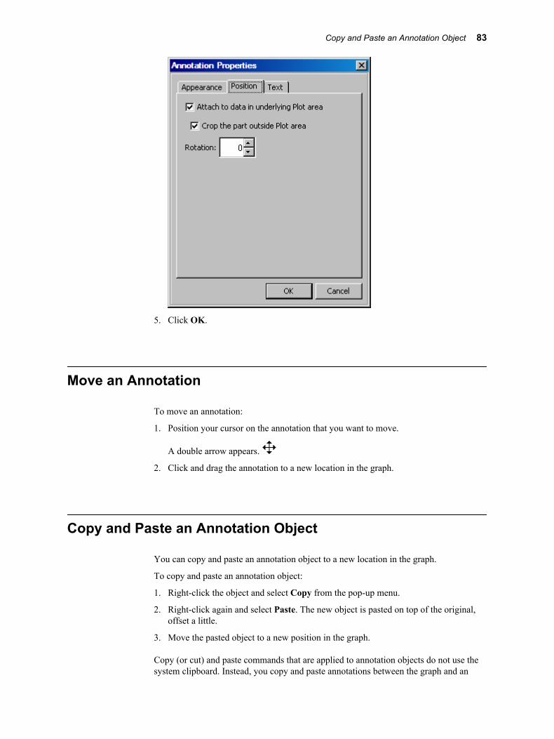
5. Click OK.
Move an Annotation
To move an annotation:
1. Position your cursor on the annotation that you want to move.
A double arrow appears.
2. Click and drag the annotation to a new location in the graph.
Copy and Paste an Annotation Object
You can copy and paste an annotation object to a new location in the graph.
To copy and paste an annotation object:
1. Right-click the object and select Copy from the pop-up menu.
2. Right-click again and select Paste. The new object is pasted on top of the original,offset a little.
3. Move the pasted object to a new position in the graph.
Copy (or cut) and paste commands that are applied to annotation objects do not use thesystem clipboard. Instead, you copy and paste annotations between the graph and an
Copy and Paste an Annotation Object 83
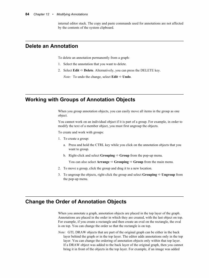
internal editor stack. The copy and paste commands used for annotations are not affectedby the contents of the system clipboard.
Delete an Annotation
To delete an annotation permanently from a graph:
1. Select the annotation that you want to delete.
2. Select Edit ð Delete. Alternatively, you can press the DELETE key.
Note: To undo the change, select Edit ð Undo.
Working with Groups of Annotation Objects
When you group annotation objects, you can easily move all items in the group as oneobject.
You cannot work on an individual object if it is part of a group. For example, in order tomodify the text of a member object, you must first ungroup the objects.
To create and work with groups:
1. To create a group:
a. Press and hold the CTRL key while you click on the annotation objects that youwant to group.
b. Right-click and select Grouping ð Group from the pop-up menu.
You can also select Arrange ð Grouping ð Group from the main menu.
2. To move a group, click the group and drag it to a new location.
3. To ungroup the objects, right-click the group and select Grouping ð Ungroup fromthe pop-up menu.
Change the Order of Annotation Objects
When you annotate a graph, annotation objects are placed in the top layer of the graph.Annotations are placed in the order in which they are created, with the last object on top.For example, if you create a rectangle and then create an oval on the rectangle, the ovalis on top. You can change the order so that the rectangle is on top.
Note: GTL DRAW objects that are part of the original graph can be either in the backlayer behind the graph or in the top layer. The editor adds annotations only in the toplayer. You can change the ordering of annotation objects only within that top layer.If a DRAW object was added to the back layer of the original graph, then you cannotbring it in front of the objects in the top layer. For example, if an image was added
84 Chapter 12 • Modifying Annotations
using DrawImage(layer=back), then the image cannot be moved in front of objects inthe top layer.
To change the order of an annotation object:
1. Right-click the object and select Order from the pop-up menu.
You can also select Arrange ð Order from the main menu.
2. From the cascading menu, select one of the following options:
• Bring to Front moves the selected object forward to the top of the stack.
• Bring Forward moves the selected object forward one layer in the stack.
• Send to Back moves the selected object to the bottom of the stack.
• Send Backward moves the selected object back one layer in the stack.
Align Multiple Annotation Objects
You can specify that a group of annotations be left-aligned, centered, right-aligned, andso on.
To align multiple annotation objects:
1. Press and hold the CTRL Key while you click on the objects to be aligned. The firstobject clicked is used as a reference object. The reference object stays in its place,and the other objects are moved to align with it.
2. From the main menu, select Arrange ð Align.
You can also select Arrange ð Align from the main menu.
3. From the cascading menu, select your alignment:
• Top aligns all selected objects with the top edge of the reference object.
• Bottom aligns all selected objects with the bottom edge of the reference object.
• Left aligns all selected objects with the left edge of the reference object.
• Right aligns all selected objects with the right edge of the reference object.
• Center aligns all selected objects around the center of the reference object.
Align Multiple Annotation Objects 85

86 Chapter 12 • Modifying Annotations
Part 4
Examples
Chapter 13Editing and Annotating a Simple Graph by Example . . . . . . . . . . . . . . 89
Chapter 14Showing and Hiding Labels By Example . . . . . . . . . . . . . . . . . . . . . . . . . 97
Chapter 15Modifying a Multi-Cell Graph By Example . . . . . . . . . . . . . . . . . . . . . . . 101
Chapter 16Editing and Annotating a SAS/STAT Graph By Example . . . . . . . . . 109
87

88
Chapter 13
Editing and Annotating a SimpleGraph by Example
About the Simple Graph . . . . . . . . . . . . . . . . . . . . . . . . . . . . . . . . . . . . . . . . . . . . . . . 89
Code for the Simple Graph Example . . . . . . . . . . . . . . . . . . . . . . . . . . . . . . . . . . . . . 90
Editing the Graph . . . . . . . . . . . . . . . . . . . . . . . . . . . . . . . . . . . . . . . . . . . . . . . . . . . . . 90Add a Title to the Graph . . . . . . . . . . . . . . . . . . . . . . . . . . . . . . . . . . . . . . . . . . . . . . 90Change the Axis Labels for the Graph . . . . . . . . . . . . . . . . . . . . . . . . . . . . . . . . . . . 90Change the Marker Symbol and Size . . . . . . . . . . . . . . . . . . . . . . . . . . . . . . . . . . . . 91Change the Graph Style . . . . . . . . . . . . . . . . . . . . . . . . . . . . . . . . . . . . . . . . . . . . . . 91Change the Size of the Graph . . . . . . . . . . . . . . . . . . . . . . . . . . . . . . . . . . . . . . . . . . 91View Your Changes . . . . . . . . . . . . . . . . . . . . . . . . . . . . . . . . . . . . . . . . . . . . . . . . . 92
Annotating the Graph . . . . . . . . . . . . . . . . . . . . . . . . . . . . . . . . . . . . . . . . . . . . . . . . . 93Add a Line Annotation to the Graph . . . . . . . . . . . . . . . . . . . . . . . . . . . . . . . . . . . . 93Add Text to the Graph . . . . . . . . . . . . . . . . . . . . . . . . . . . . . . . . . . . . . . . . . . . . . . . 94View Your Annotation Changes . . . . . . . . . . . . . . . . . . . . . . . . . . . . . . . . . . . . . . . . 94
About the Simple GraphThis example uses the Class data set in the SAS Help library. The example provides theheight and weight of individual students in a class and uses the SGPLOT procedure toproduce a scatter plot.
In this example, you edit the graph by adding a title and changing the axis labels. Youalso change the scatter plot markers, the graph style, and the graph size.
89
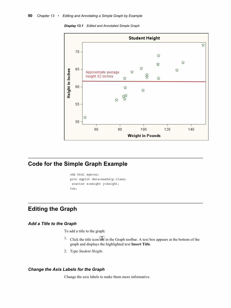
Display 13.1 Edited and Annotated Simple Graph
Code for the Simple Graph Exampleods html sge=on;proc sgplot data=sashelp.class; scatter x=weight y=height;run;
Editing the Graph
Add a Title to the GraphTo add a title to the graph:
1. Click the title icon in the Graph toolbar. A text box appears at the bottom of thegraph and displays the highlighted text Insert Title.
2. Type Student Height.
Change the Axis Labels for the GraphChange the axis labels to make them more informative.
90 Chapter 13 • Editing and Annotating a Simple Graph by Example
To change the axis labels:
1. Double-click the Y axis label (Height) and change the text to Height in Inches.
2. Double-click the X axis label (Weight) and change the text to Weight in Pounds.
Change the Marker Symbol and SizeWhen you change the marker for the data points, you modify plot properties.
To change the markers:
1. Right-click inside the plot and select Plot Properties. The Plot Properties dialog boxappears.
2. On the Plots tab, select the unfilled star marker ( ) from the Symbol list box.
3. Select 9 from the Size list box.
4. Click OK.
Change the Graph StyleThe default style for the graph is StatGraphScheme, which inherits attributes from thestyle that was used when the graph was created (in this example, HTMLBlue). In thisstep, you change the style to Analysis.
1. Select Format ð Style from the main menu.
2. From the cascading menu, select Analysis.
Notice that the color of the markers has changed, but the marker symbol and size remainthe same as they were. The reason is that you explicitly changed the marker symbol andsize. The marker attributes that you specified override the settings that are associatedwith the new style.
Change the Size of the GraphIn this example, you want the graph to be five inches by approximately three inches inorder to fit in a color presentation.
To change the size:
1. Right-click the graph and select Graph Properties. The Graph Properties dialog boxappears.
Editing the Graph 91
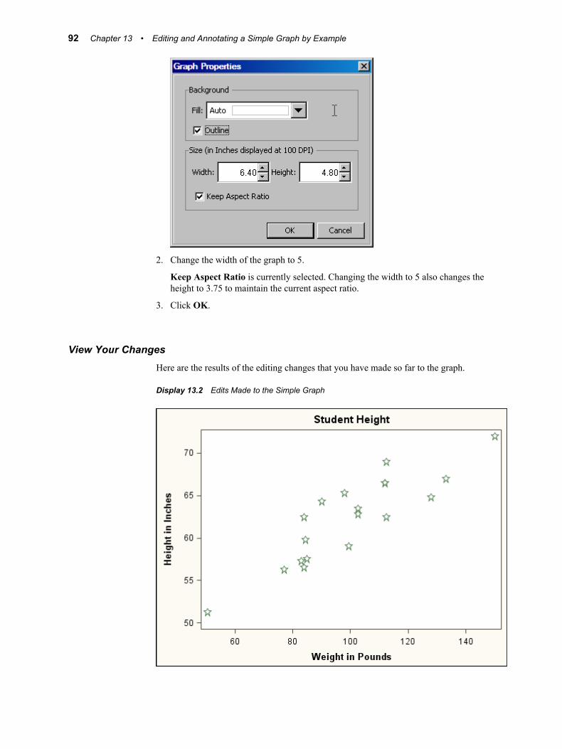
2. Change the width of the graph to 5.
Keep Aspect Ratio is currently selected. Changing the width to 5 also changes theheight to 3.75 to maintain the current aspect ratio.
3. Click OK.
View Your ChangesHere are the results of the editing changes that you have made so far to the graph.
Display 13.2 Edits Made to the Simple Graph
92 Chapter 13 • Editing and Annotating a Simple Graph by Example
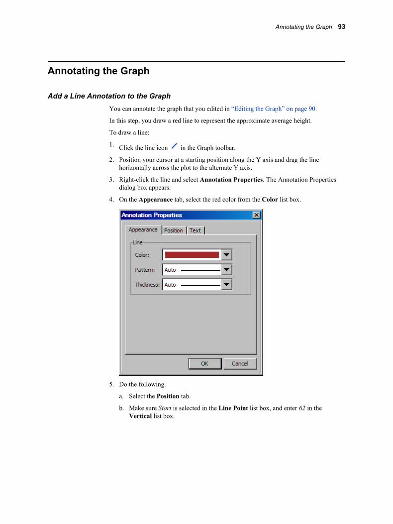
Annotating the Graph
Add a Line Annotation to the GraphYou can annotate the graph that you edited in “Editing the Graph” on page 90.
In this step, you draw a red line to represent the approximate average height.
To draw a line:
1. Click the line icon in the Graph toolbar.
2. Position your cursor at a starting position along the Y axis and drag the linehorizontally across the plot to the alternate Y axis.
3. Right-click the line and select Annotation Properties. The Annotation Propertiesdialog box appears.
4. On the Appearance tab, select the red color from the Color list box.
5. Do the following.
a. Select the Position tab.
b. Make sure Start is selected in the Line Point list box, and enter 62 in theVertical list box.
Annotating the Graph 93
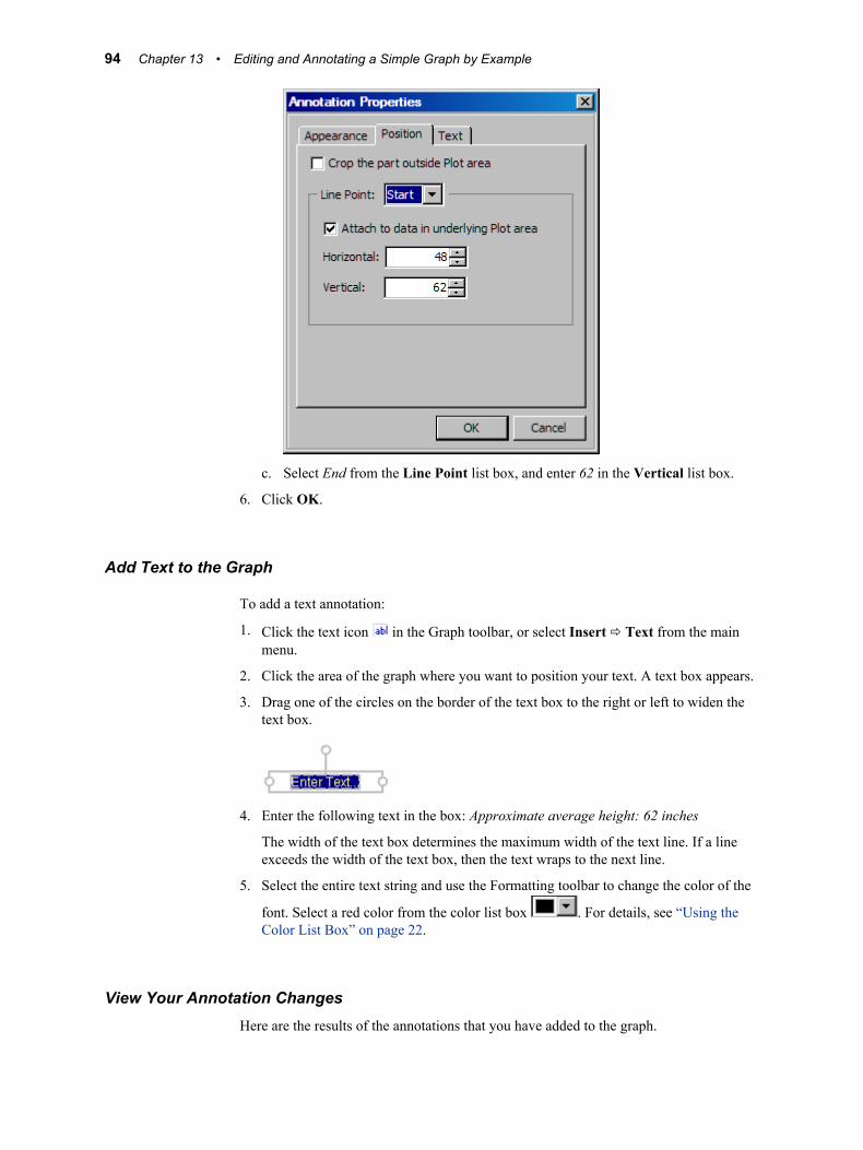
c. Select End from the Line Point list box, and enter 62 in the Vertical list box.
6. Click OK.
Add Text to the Graph
To add a text annotation:
1. Click the text icon in the Graph toolbar, or select Insert ð Text from the mainmenu.
2. Click the area of the graph where you want to position your text. A text box appears.
3. Drag one of the circles on the border of the text box to the right or left to widen thetext box.
4. Enter the following text in the box: Approximate average height: 62 inches
The width of the text box determines the maximum width of the text line. If a lineexceeds the width of the text box, then the text wraps to the next line.
5. Select the entire text string and use the Formatting toolbar to change the color of the
font. Select a red color from the color list box . For details, see “Using theColor List Box” on page 22.
View Your Annotation ChangesHere are the results of the annotations that you have added to the graph.
94 Chapter 13 • Editing and Annotating a Simple Graph by Example
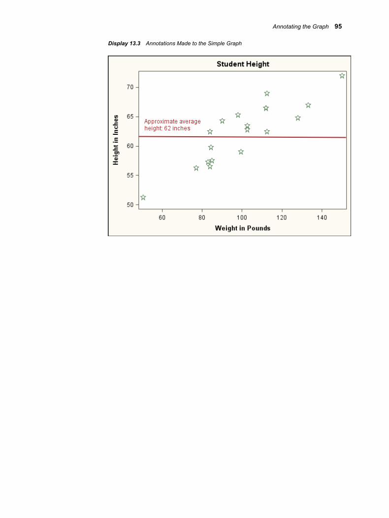
Display 13.3 Annotations Made to the Simple Graph
Annotating the Graph 95

96 Chapter 13 • Editing and Annotating a Simple Graph by Example
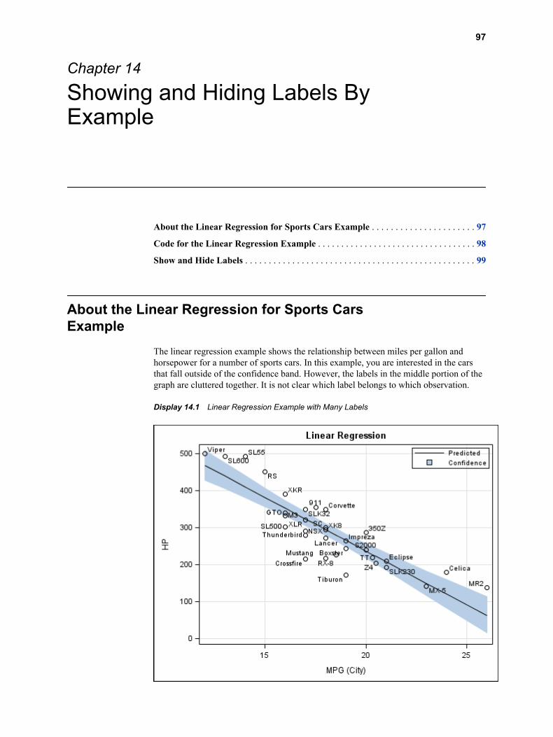
Chapter 14
Showing and Hiding Labels ByExample
About the Linear Regression for Sports Cars Example . . . . . . . . . . . . . . . . . . . . . . 97
Code for the Linear Regression Example . . . . . . . . . . . . . . . . . . . . . . . . . . . . . . . . . . 98
Show and Hide Labels . . . . . . . . . . . . . . . . . . . . . . . . . . . . . . . . . . . . . . . . . . . . . . . . . 99
About the Linear Regression for Sports CarsExample
The linear regression example shows the relationship between miles per gallon andhorsepower for a number of sports cars. In this example, you are interested in the carsthat fall outside of the confidence band. However, the labels in the middle portion of thegraph are cluttered together. It is not clear which label belongs to which observation.
Display 14.1 Linear Regression Example with Many Labels
97
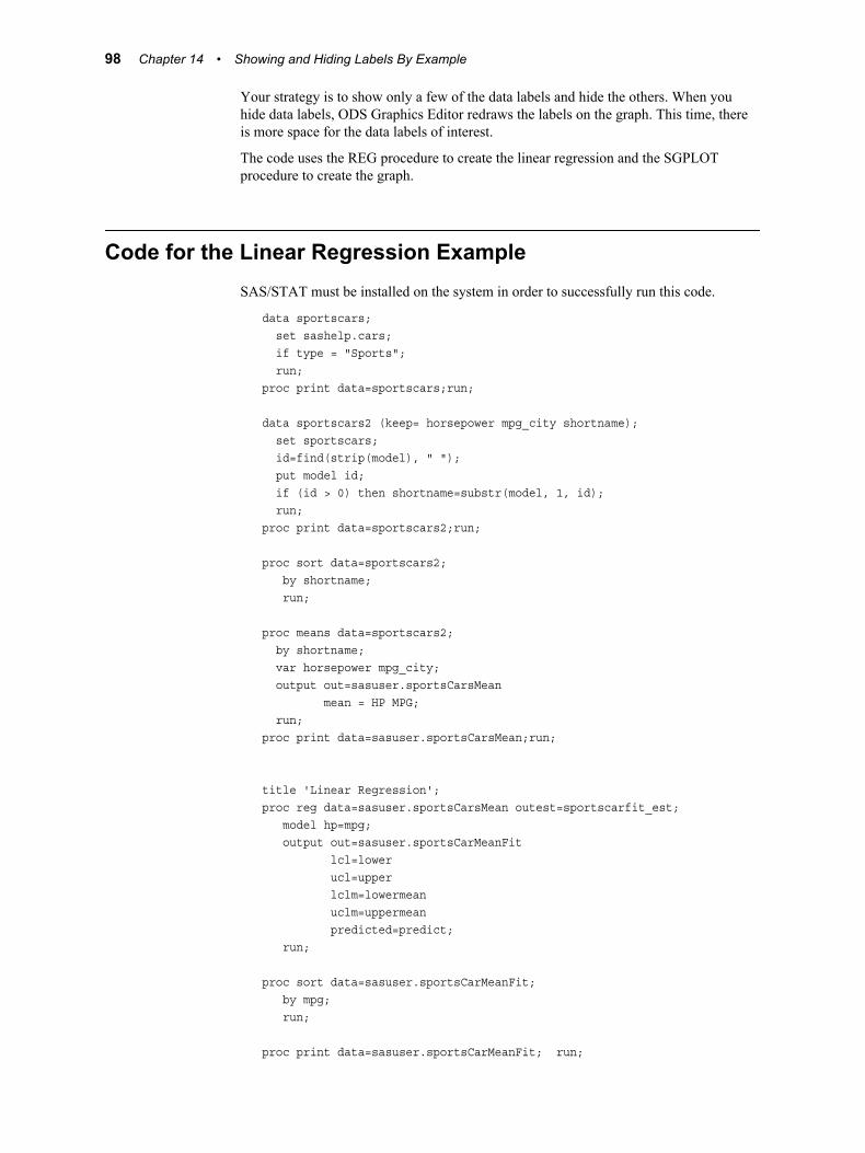
Your strategy is to show only a few of the data labels and hide the others. When youhide data labels, ODS Graphics Editor redraws the labels on the graph. This time, thereis more space for the data labels of interest.
The code uses the REG procedure to create the linear regression and the SGPLOTprocedure to create the graph.
Code for the Linear Regression ExampleSAS/STAT must be installed on the system in order to successfully run this code.
data sportscars; set sashelp.cars; if type = "Sports"; run;proc print data=sportscars;run;
data sportscars2 (keep= horsepower mpg_city shortname); set sportscars; id=find(strip(model), " "); put model id; if (id > 0) then shortname=substr(model, 1, id); run;proc print data=sportscars2;run;
proc sort data=sportscars2; by shortname; run;
proc means data=sportscars2; by shortname; var horsepower mpg_city; output out=sasuser.sportsCarsMean mean = HP MPG; run;proc print data=sasuser.sportsCarsMean;run;
title 'Linear Regression';proc reg data=sasuser.sportsCarsMean outest=sportscarfit_est; model hp=mpg; output out=sasuser.sportsCarMeanFit lcl=lower ucl=upper lclm=lowermean uclm=uppermean predicted=predict; run;
proc sort data=sasuser.sportsCarMeanFit; by mpg; run;
proc print data=sasuser.sportsCarMeanFit; run;
98 Chapter 14 • Showing and Hiding Labels By Example
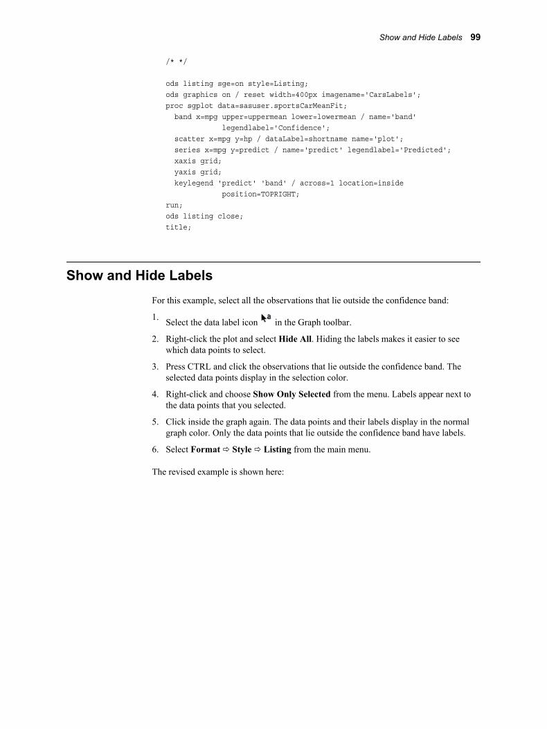
/* */
ods listing sge=on style=Listing;ods graphics on / reset width=400px imagename='CarsLabels';proc sgplot data=sasuser.sportsCarMeanFit; band x=mpg upper=uppermean lower=lowermean / name='band' legendlabel='Confidence'; scatter x=mpg y=hp / dataLabel=shortname name='plot'; series x=mpg y=predict / name='predict' legendlabel='Predicted'; xaxis grid; yaxis grid; keylegend 'predict' 'band' / across=1 location=inside position=TOPRIGHT;run; ods listing close;title;
Show and Hide LabelsFor this example, select all the observations that lie outside the confidence band:
1. Select the data label icon in the Graph toolbar.
2. Right-click the plot and select Hide All. Hiding the labels makes it easier to seewhich data points to select.
3. Press CTRL and click the observations that lie outside the confidence band. Theselected data points display in the selection color.
4. Right-click and choose Show Only Selected from the menu. Labels appear next tothe data points that you selected.
5. Click inside the graph again. The data points and their labels display in the normalgraph color. Only the data points that lie outside the confidence band have labels.
6. Select Format ð Style ð Listing from the main menu.
The revised example is shown here:
Show and Hide Labels 99
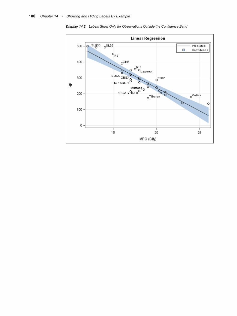
Display 14.2 Labels Show Only for Observations Outside the Confidence Band
100 Chapter 14 • Showing and Hiding Labels By Example
Chapter 15
Modifying a Multi-Cell Graph ByExample
Modifying a Multi-Cell Graph That Uses a Single Data Set . . . . . . . . . . . . . . . . . 101About the Classification Panel Example . . . . . . . . . . . . . . . . . . . . . . . . . . . . . . . . 101Code for the Classification Panel Example . . . . . . . . . . . . . . . . . . . . . . . . . . . . . . 102Modify the Classification Panel Example . . . . . . . . . . . . . . . . . . . . . . . . . . . . . . . 102
Modifying Individual Plots in a Diagnostic Panel . . . . . . . . . . . . . . . . . . . . . . . . . . 104About the Fitness Example . . . . . . . . . . . . . . . . . . . . . . . . . . . . . . . . . . . . . . . . . . . 104Code for the Fitness Example . . . . . . . . . . . . . . . . . . . . . . . . . . . . . . . . . . . . . . . . . 105Modify the Fitness Example . . . . . . . . . . . . . . . . . . . . . . . . . . . . . . . . . . . . . . . . . . 106
Modifying a Multi-Cell Graph That Uses a SingleData Set
About the Classification Panel ExampleThis example uses the Heart data set in the SAS Help library. The example provides thecholesterol distribution for a group of men and women. The code uses the SGPANELprocedure to create a classification panel with two cells. Both cells are driven by thesame data set.
101
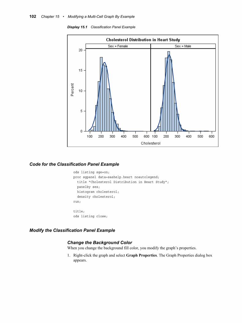
Display 15.1 Classification Panel Example
Code for the Classification Panel Exampleods listing sge=on;proc sgpanel data=sashelp.heart noautolegend; title "Cholesterol Distribution in Heart Study"; panelby sex; histogram cholesterol; density cholesterol;run;
title;ods listing close;
Modify the Classification Panel Example
Change the Background ColorWhen you change the background fill color, you modify the graph’s properties.
1. Right-click the graph and select Graph Properties. The Graph Properties dialog boxappears.
102 Chapter 15 • Modifying a Multi-Cell Graph By Example
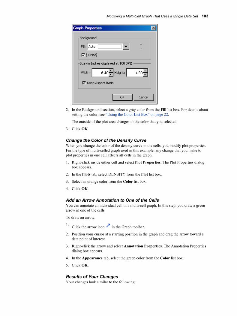
2. In the Background section, select a gray color from the Fill list box. For details aboutsetting the color, see “Using the Color List Box” on page 22.
The outside of the plot area changes to the color that you selected.
3. Click OK.
Change the Color of the Density CurveWhen you change the color of the density curve in the cells, you modify plot properties.For the type of multi-celled graph used in this example, any change that you make toplot properties in one cell affects all cells in the graph.
1. Right-click inside either cell and select Plot Properties. The Plot Properties dialogbox appears.
2. In the Plots tab, select DENSITY from the Plot list box.
3. Select an orange color from the Color list box.
4. Click OK.
Add an Arrow Annotation to One of the CellsYou can annotate an individual cell in a multi-cell graph. In this step, you draw a greenarrow in one of the cells.
To draw an arrow:
1. Click the arrow icon in the Graph toolbar.
2. Position your cursor at a starting position in the graph and drag the arrow toward adata point of interest.
3. Right-click the arrow and select Annotation Properties. The Annotation Propertiesdialog box appears.
4. In the Appearance tab, select the green color from the Color list box.
5. Click OK.
Results of Your ChangesYour changes look similar to the following:
Modifying a Multi-Cell Graph That Uses a Single Data Set 103
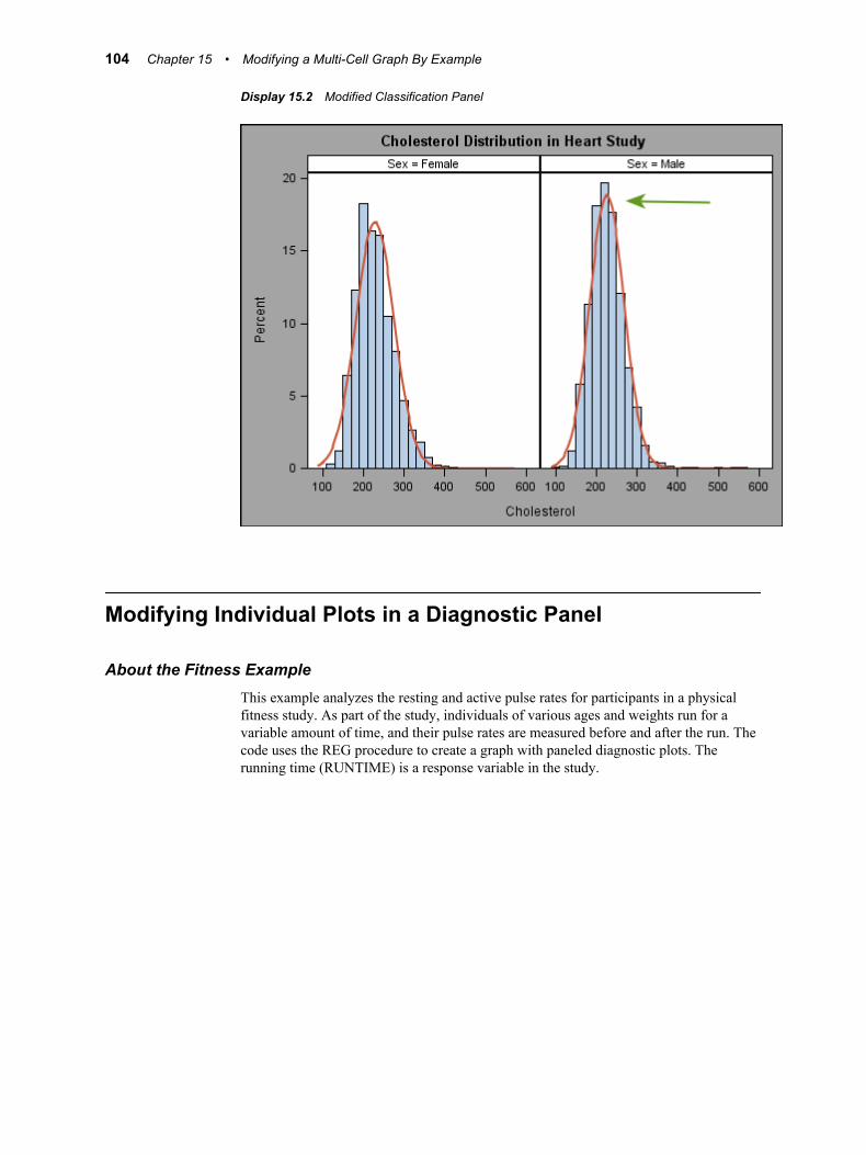
Display 15.2 Modified Classification Panel
Modifying Individual Plots in a Diagnostic Panel
About the Fitness ExampleThis example analyzes the resting and active pulse rates for participants in a physicalfitness study. As part of the study, individuals of various ages and weights run for avariable amount of time, and their pulse rates are measured before and after the run. Thecode uses the REG procedure to create a graph with paneled diagnostic plots. Therunning time (RUNTIME) is a response variable in the study.
104 Chapter 15 • Modifying a Multi-Cell Graph By Example
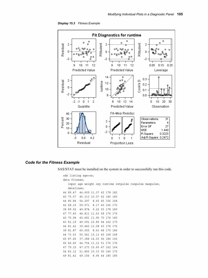
Display 15.3 Fitness Example
Code for the Fitness ExampleSAS/STAT must be installed on the system in order to successfully run this code.
ods listing sge=on;data fitness; input age weight oxy runtime rstpulse runpulse maxpulse; datalines;44 89.47 44.609 11.37 62 178 18240 75.07 45.313 10.07 62 185 18544 85.84 54.297 8.65 45 156 16842 68.15 59.571 8.17 40 166 17238 89.02 49.874 9.22 55 178 18047 77.45 44.811 11.63 58 176 17640 75.98 45.681 11.95 70 176 18043 81.19 49.091 10.85 64 162 17044 81.42 39.442 13.08 63 174 17638 81.87 60.055 8.63 48 170 18644 73.03 50.541 10.13 45 168 16845 87.66 37.388 14.03 56 186 19245 66.45 44.754 11.12 51 176 17647 79.15 47.273 10.60 47 162 16454 83.12 51.855 10.33 50 166 17049 81.42 49.156 8.95 44 180 185
Modifying Individual Plots in a Diagnostic Panel 105
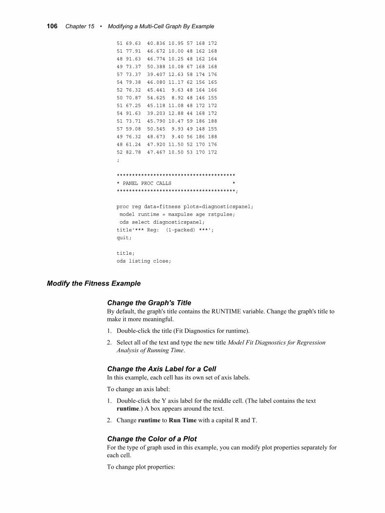
51 69.63 40.836 10.95 57 168 17251 77.91 46.672 10.00 48 162 16848 91.63 46.774 10.25 48 162 16449 73.37 50.388 10.08 67 168 16857 73.37 39.407 12.63 58 174 17654 79.38 46.080 11.17 62 156 16552 76.32 45.441 9.63 48 164 16650 70.87 54.625 8.92 48 146 15551 67.25 45.118 11.08 48 172 17254 91.63 39.203 12.88 44 168 17251 73.71 45.790 10.47 59 186 18857 59.08 50.545 9.93 49 148 15549 76.32 48.673 9.40 56 186 18848 61.24 47.920 11.50 52 170 17652 82.78 47.467 10.50 53 170 172;
**************************************** PANEL PROC CALLS ****************************************;
proc reg data=fitness plots=diagnosticspanel; model runtime = maxpulse age rstpulse; ods select diagnosticspanel;title'*** Reg: (1-packed) ***';quit;
title;ods listing close;
Modify the Fitness Example
Change the Graph's TitleBy default, the graph's title contains the RUNTIME variable. Change the graph's title tomake it more meaningful.
1. Double-click the title (Fit Diagnostics for runtime).
2. Select all of the text and type the new title Model Fit Diagnostics for RegressionAnalysis of Running Time.
Change the Axis Label for a CellIn this example, each cell has its own set of axis labels.
To change an axis label:
1. Double-click the Y axis label for the middle cell. (The label contains the textruntime.) A box appears around the text.
2. Change runtime to Run Time with a capital R and T.
Change the Color of a PlotFor the type of graph used in this example, you can modify plot properties separately foreach cell.
To change plot properties:
106 Chapter 15 • Modifying a Multi-Cell Graph By Example
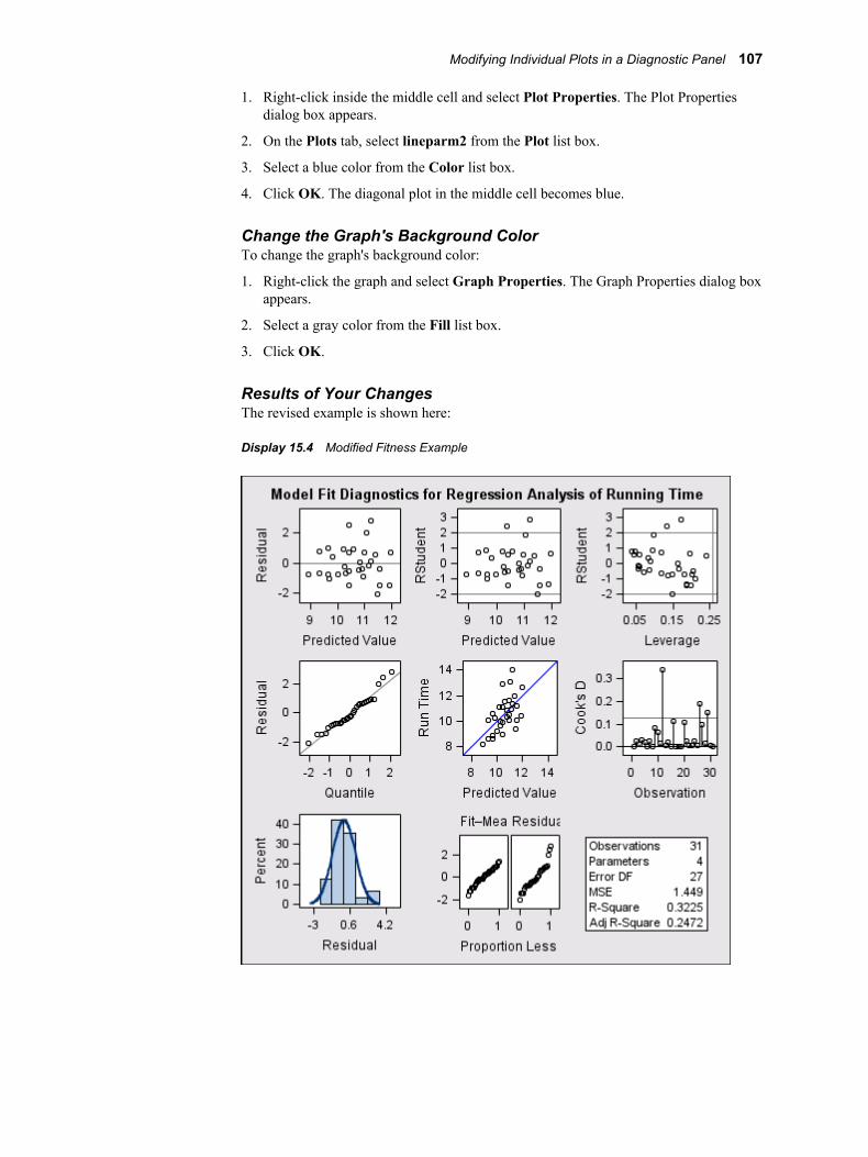
1. Right-click inside the middle cell and select Plot Properties. The Plot Propertiesdialog box appears.
2. On the Plots tab, select lineparm2 from the Plot list box.
3. Select a blue color from the Color list box.
4. Click OK. The diagonal plot in the middle cell becomes blue.
Change the Graph's Background ColorTo change the graph's background color:
1. Right-click the graph and select Graph Properties. The Graph Properties dialog boxappears.
2. Select a gray color from the Fill list box.
3. Click OK.
Results of Your ChangesThe revised example is shown here:
Display 15.4 Modified Fitness Example
Modifying Individual Plots in a Diagnostic Panel 107

108 Chapter 15 • Modifying a Multi-Cell Graph By Example
Chapter 16
Editing and Annotating aSAS/STAT Graph By Example
About the Economy Growth Example . . . . . . . . . . . . . . . . . . . . . . . . . . . . . . . . . . . 109
Code for the Economy Example . . . . . . . . . . . . . . . . . . . . . . . . . . . . . . . . . . . . . . . . 110
Editing the Graph . . . . . . . . . . . . . . . . . . . . . . . . . . . . . . . . . . . . . . . . . . . . . . . . . . . . 112Change the Graph's Title . . . . . . . . . . . . . . . . . . . . . . . . . . . . . . . . . . . . . . . . . . . . 112Add a Footnote to the Graph . . . . . . . . . . . . . . . . . . . . . . . . . . . . . . . . . . . . . . . . . 112Move the Legend . . . . . . . . . . . . . . . . . . . . . . . . . . . . . . . . . . . . . . . . . . . . . . . . . . 112Change the Line Pattern . . . . . . . . . . . . . . . . . . . . . . . . . . . . . . . . . . . . . . . . . . . . . 113
Adding Annotations to Highlight Outlier Data . . . . . . . . . . . . . . . . . . . . . . . . . . . . 114Add an Oval to the Outlier . . . . . . . . . . . . . . . . . . . . . . . . . . . . . . . . . . . . . . . . . . . 114Change the Color of the Oval . . . . . . . . . . . . . . . . . . . . . . . . . . . . . . . . . . . . . . . . . 114Draw an Arrow That Points to the Outlier . . . . . . . . . . . . . . . . . . . . . . . . . . . . . . . 115Add Text to the Arrow . . . . . . . . . . . . . . . . . . . . . . . . . . . . . . . . . . . . . . . . . . . . . . 115
Preparing The Graph for Presentation . . . . . . . . . . . . . . . . . . . . . . . . . . . . . . . . . . 115Change the Graph's Style . . . . . . . . . . . . . . . . . . . . . . . . . . . . . . . . . . . . . . . . . . . . 115Change the Size of the Graph . . . . . . . . . . . . . . . . . . . . . . . . . . . . . . . . . . . . . . . . . 115
Viewing and Saving the Results of Your Changes . . . . . . . . . . . . . . . . . . . . . . . . . . 116Results of Your Changes to the Graph . . . . . . . . . . . . . . . . . . . . . . . . . . . . . . . . . . 116Save Your Changes . . . . . . . . . . . . . . . . . . . . . . . . . . . . . . . . . . . . . . . . . . . . . . . . . 117
About the Economy Growth ExampleThe Economy Growth example uses the Distance by Distance graph, which is generatedusing the ROBUSTREG procedure. The main purpose of robust regression is to detectoutliers and leverage points and to provide stable results in the presence of suchinfluential points.
109
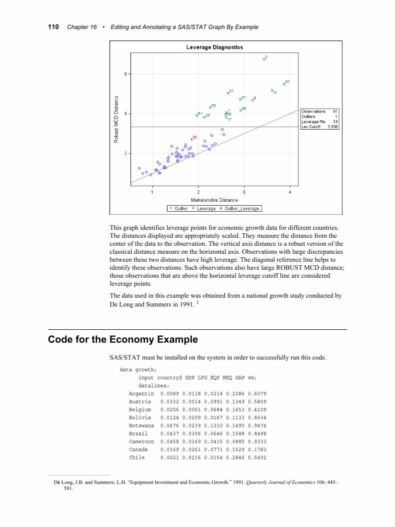
This graph identifies leverage points for economic growth data for different countries.The distances displayed are appropriately scaled. They measure the distance from thecenter of the data to the observation. The vertical axis distance is a robust version of theclassical distance measure on the horizontal axis. Observations with large discrepanciesbetween these two distances have high leverage. The diagonal reference line helps toidentify these observations. Such observations also have large ROBUST MCD distance;those observations that are above the horizontal leverage cutoff line are consideredleverage points.
The data used in this example was obtained from a national growth study conducted byDe Long and Summers in 1991. 1
Code for the Economy ExampleSAS/STAT must be installed on the system in order to successfully run this code.
data growth; input country$ GDP LFG EQP NEQ GAP @@; datalines; Argentin 0.0089 0.0118 0.0214 0.2286 0.6079 Austria 0.0332 0.0014 0.0991 0.1349 0.5809 Belgium 0.0256 0.0061 0.0684 0.1653 0.4109 Bolivia 0.0124 0.0209 0.0167 0.1133 0.8634 Botswana 0.0676 0.0239 0.1310 0.1490 0.9474 Brazil 0.0437 0.0306 0.0646 0.1588 0.8498 Cameroon 0.0458 0.0169 0.0415 0.0885 0.9333 Canada 0.0169 0.0261 0.0771 0.1529 0.1783 Chile 0.0021 0.0216 0.0154 0.2846 0.5402
1De Long, J.B. and Summers, L.H. “Equipment Investment and Economic Growth.” 1991. Quarterly Journal of Economics 106: 445–501.
110 Chapter 16 • Editing and Annotating a SAS/STAT Graph By Example
Colombia 0.0239 0.0266 0.0229 0.1553 0.7695 CostaRic 0.0121 0.0354 0.0433 0.1067 0.7043 Denmark 0.0187 0.0115 0.0688 0.1834 0.4079 Dominica 0.0199 0.0280 0.0321 0.1379 0.8293 Ecuador 0.0283 0.0274 0.0303 0.2097 0.8205 ElSalvad 0.0046 0.0316 0.0223 0.0577 0.8414 Ethiopia 0.0094 0.0206 0.0212 0.0288 0.9805 Finland 0.0301 0.0083 0.1206 0.2494 0.5589 France 0.0292 0.0089 0.0879 0.1767 0.4708 Germany 0.0259 0.0047 0.0890 0.1885 0.4585 Greece 0.0446 0.0044 0.0655 0.2245 0.7924 Guatemal 0.0149 0.0242 0.0384 0.0516 0.7885 Honduras 0.0148 0.0303 0.0446 0.0954 0.8850 HongKong 0.0484 0.0359 0.0767 0.1233 0.7471 India 0.0115 0.0170 0.0278 0.1448 0.9356 Indonesi 0.0345 0.0213 0.0221 0.1179 0.9243 Ireland 0.0288 0.0081 0.0814 0.1879 0.6457 Israel 0.0452 0.0305 0.1112 0.1788 0.6816 Italy 0.0362 0.0038 0.0683 0.1790 0.5441 IvoryCoa 0.0278 0.0274 0.0243 0.0957 0.9207 Jamaica 0.0055 0.0201 0.0609 0.1455 0.8229 Japan 0.0535 0.0117 0.1223 0.2464 0.7484 Kenya 0.0146 0.0346 0.0462 0.1268 0.9415 Korea 0.0479 0.0282 0.0557 0.1842 0.8807 Luxembou 0.0236 0.0064 0.0711 0.1944 0.2863 Madagasc -0.0102 0.0203 0.0219 0.0481 0.9217 Malawi 0.0153 0.0226 0.0361 0.0935 0.9628 Malaysia 0.0332 0.0316 0.0446 0.1878 0.7853 Mali 0.0044 0.0184 0.0433 0.0267 0.9478 Mexico 0.0198 0.0349 0.0273 0.1687 0.5921 Morocco 0.0243 0.0281 0.0260 0.0540 0.8405 Netherla 0.0231 0.0146 0.0778 0.1781 0.3605 Nigeria -0.0047 0.0283 0.0358 0.0842 0.8579 Norway 0.0260 0.0150 0.0701 0.2199 0.3755 Pakistan 0.0295 0.0258 0.0263 0.0880 0.9180 Panama 0.0295 0.0279 0.0388 0.2212 0.8015 Paraguay 0.0261 0.0299 0.0189 0.1011 0.8458 Peru 0.0107 0.0271 0.0267 0.0933 0.7406 Philippi 0.0179 0.0253 0.0445 0.0974 0.8747 Portugal 0.0318 0.0118 0.0729 0.1571 0.8033 Senegal -0.0011 0.0274 0.0193 0.0807 0.8884 Spain 0.0373 0.0069 0.0397 0.1305 0.6613 SriLanka 0.0137 0.0207 0.0138 0.1352 0.8555 Tanzania 0.0184 0.0276 0.0860 0.0940 0.9762 Thailand 0.0341 0.0278 0.0395 0.1412 0.9174 Tunisia 0.0279 0.0256 0.0428 0.0972 0.7838 U.K. 0.0189 0.0048 0.0694 0.1132 0.4307 U.S. 0.0133 0.0189 0.0762 0.1356 0.0000 Uruguay 0.0041 0.0052 0.0155 0.1154 0.5782 Venezuel 0.0120 0.0378 0.0340 0.0760 0.4974 Zambia -0.0110 0.0275 0.0702 0.2012 0.8695 Zimbabwe 0.0110 0.0309 0.0843 0.1257 0.8875 ;
ods listing sge=on;
Code for the Economy Example 111
ods select "Distance by Distance";
proc robustreg data=growth plot=all method=lts; model GDP = LFG GAP EQP NEQ / diagnostics(all); run;
ods listing close;title;
Editing the Graph
Change the Graph's TitleChange the graph's title to make it more meaningful to your target audience.
1. Double-click the title (Leverage Diagnostics).
2. Select all of the text and type the new title Analysis of Economy Growth.
Add a Footnote to the GraphAdd a footnote that shows the respective year for the data.
1. Click the footnote icon in the Graph toolbar. A text box appears at the bottom ofthe graph and displays the highlighted text Insert Footnote.
2. Type Data source: De Long and Summers (1991).
Move the LegendOnce the footnote has been added, the bottom of the graph looks crowded. Because thereis ample space available inside the plot area, move the legend into the plot in the lowerright corner.
1. Right-click the legend and select Legend Properties from the pop-up menu. TheLegend Properties dialog box appears.
112 Chapter 16 • Editing and Annotating a SAS/STAT Graph By Example
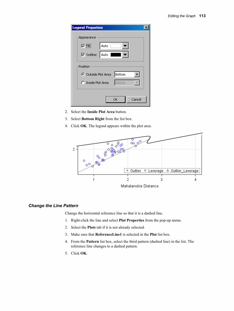
2. Select the Inside Plot Area button.
3. Select Bottom Right from the list box.
4. Click OK. The legend appears within the plot area.
Change the Line PatternChange the horizontal reference line so that it is a dashed line.
1. Right-click the line and select Plot Properties from the pop-up menu.
2. Select the Plots tab if it is not already selected.
3. Make sure that ReferenceLine1 is selected in the Plot list box.
4. From the Pattern list box, select the third pattern (dashed line) in the list. Thereference line changes to a dashed pattern.
5. Click OK.
Editing the Graph 113
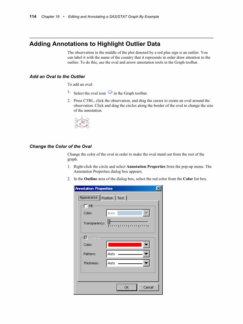
Adding Annotations to Highlight Outlier DataThe observation in the middle of the plot denoted by a red plus sign is an outlier. Youcan label it with the name of the country that it represents in order draw attention to theoutlier. To do this, use the oval and arrow annotation tools in the Graph toolbar.
Add an Oval to the OutlierTo add an oval:
1. Select the oval icon in the Graph toolbar.
2. Press CTRL, click the observation, and drag the cursor to create an oval around theobservation. Click and drag the circles along the border of the oval to change the sizeof the annotation.
Change the Color of the OvalChange the color of the oval in order to make the oval stand out from the rest of thegraph.
1. Right-click the circle and select Annotation Properties from the pop-up menu. TheAnnotation Properties dialog box appears.
2. In the Outline area of the dialog box, select the red color from the Color list box.
114 Chapter 16 • Editing and Annotating a SAS/STAT Graph By Example
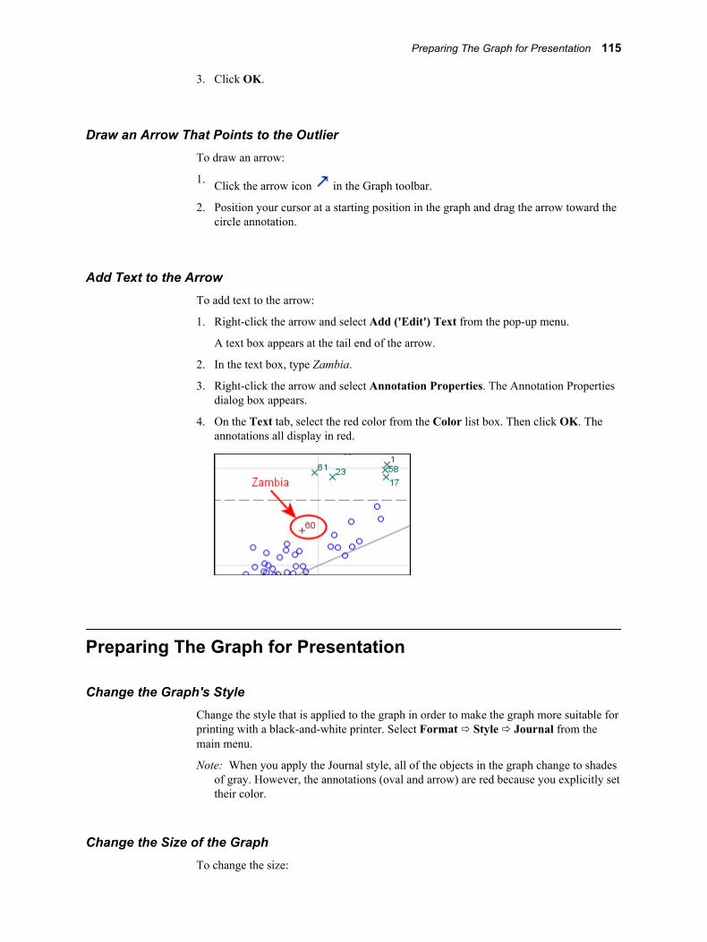
3. Click OK.
Draw an Arrow That Points to the OutlierTo draw an arrow:
1. Click the arrow icon in the Graph toolbar.
2. Position your cursor at a starting position in the graph and drag the arrow toward thecircle annotation.
Add Text to the ArrowTo add text to the arrow:
1. Right-click the arrow and select Add ('Edit') Text from the pop-up menu.
A text box appears at the tail end of the arrow.
2. In the text box, type Zambia.
3. Right-click the arrow and select Annotation Properties. The Annotation Propertiesdialog box appears.
4. On the Text tab, select the red color from the Color list box. Then click OK. Theannotations all display in red.
Preparing The Graph for Presentation
Change the Graph's StyleChange the style that is applied to the graph in order to make the graph more suitable forprinting with a black-and-white printer. Select Format ð Style ð Journal from themain menu.
Note: When you apply the Journal style, all of the objects in the graph change to shadesof gray. However, the annotations (oval and arrow) are red because you explicitly settheir color.
Change the Size of the GraphTo change the size:
Preparing The Graph for Presentation 115
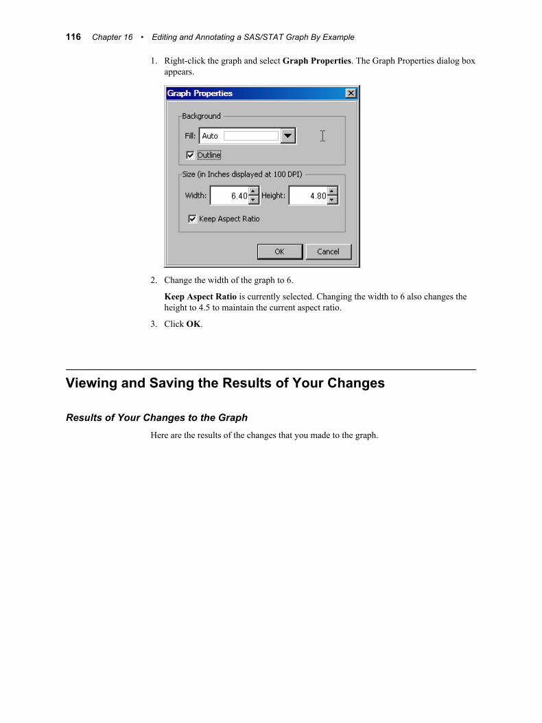
1. Right-click the graph and select Graph Properties. The Graph Properties dialog boxappears.
2. Change the width of the graph to 6.
Keep Aspect Ratio is currently selected. Changing the width to 6 also changes theheight to 4.5 to maintain the current aspect ratio.
3. Click OK.
Viewing and Saving the Results of Your Changes
Results of Your Changes to the GraphHere are the results of the changes that you made to the graph.
116 Chapter 16 • Editing and Annotating a SAS/STAT Graph By Example
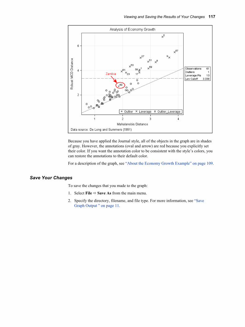
Because you have applied the Journal style, all of the objects in the graph are in shadesof gray. However, the annotations (oval and arrow) are red because you explicitly settheir color. If you want the annotation color to be consistent with the style’s colors, youcan restore the annotations to their default color.
For a description of the graph, see “About the Economy Growth Example” on page 109.
Save Your ChangesTo save the changes that you made to the graph:
1. Select File ð Save As from the main menu.
2. Specify the directory, filename, and file type. For more information, see “SaveGraph Output ” on page 11.
Viewing and Saving the Results of Your Changes 117

118 Chapter 16 • Editing and Annotating a SAS/STAT Graph By Example
Glossary
annotationa label, marker, or note that is not obtained from the data but is placed on a graphindependently. Such annotations might or might not be linked to data values in theplot.
cellin ODS graphics, a distinct rectangular subregion of a graph that can contain plots,text, or legends.
classification panela multi-cell graph in which the cell data is driven by the values of one or moreclassification variables. The number of the cells is determined by the unique valuesof the classification variables. Each cell of the panel has the same types of plots.
classification variablea variable whose values are used to group (or classify) the observations in a data setinto different groups that are meaningful for analysis. A classification variable canhave either character or numeric values. Classification variables include group,subgroup, category, and BY variables.
Graph Template Languagean extension to the Output Delivery System (ODS) that enables users to createsophisticated analytical graphs. Short form: GTL.
GTLSee Graph Template Language.
localea setting that reflects the language, local conventions, and culture for a geographicregion. Local conventions can include specific formatting rules for paper sizes, dates,times, and numbers, and a currency symbol for the country or region. Someexamples of locale values are French_Canada,Portuguese_Brazil, andChinese_Singapore.
markera symbol such as a diamond, a circle, or a triangle that is used to indicate the locationof, or annotate, a data point in a plot or graph.
ODSSee Output Delivery System.
119
ODS Graphicsan extension to ODS that is used to create analytical graphs using the GraphTemplate Language.
ODS stylea template that specifies instructions for the presentation aspects (color, font face,font size, and so on) of your SAS output. This template determines the overallappearance of the documents that use it. Each style definition consists of styleelements.
ODS templatea description of how output should appear when it is formatted. ODS templates arestored as compiled entries in a template store (item store). Common template typesinclude STATGRAPH, STYLE, CROSSTABS, TAGSET, and TABLE.
outliera data point that differs from the general trend of the data by more than is expectedby chance alone. An outlier might be an erroneous data point or one that is not fromthe same sampling model as the rest of the data.
Output Delivery Systema component of SAS software that can produce output in a variety of formats such asmarkup languages (HTML, XML), PDF, listing, RTF, PostScript, other formats, andSAS data sets.
panela graph with multiple cells.
plota visual representation of data such as a scatter plot, a series line, or a histogram.Multiple plots can be overlaid in a cell to create a graph.
scatter plot matrixa grid of scatter plots showing pairwise combinations of multiple numeric variables.
SGE filea file created in the ODS Graphics environment that contains an editable graph. Suchfiles have a .SGE file extension and can be edited only with the ODS GraphicsEditor. You can edit SGE files from the SAS Results window or by opening the SGEfile from within the ODS Graphics Editor.
120 Glossary
Index
Aabout ODS Graphics Editor 3aligning annotations 85alternate short text 25annotating graphs
add text to objects 75align objects 85annotation concepts 45change data attachment properties 57copy and paste objects 83delete objects 84group objects 84GTL annotations 6images 66lines and arrows 62markers 65move objects 83order objects in layers 84ovals (and circles) 64rectangles (and squares) 64resize objects 79rotate objects 81text annotations 61
annotation concepts 45annotation objects 45arrows 62axis labels 36
grid lines 36turn on and off 36
Ccell 5circles
See ovalscolor, changing
data 32graph background 17plot background 32
colors, specifying 22components of a graph 5
conceptsannotation 45editing 6
copy and pasteannotation object 83graph 12
Ddata attachment
change properties 57concepts 45
data labels, show or hide 39delete an annotation 84
Eedit a graph 9editable graphs 8editing concepts 6editing graphs
change background color 17plot properties 31resize a graph 16show or hide data labels 39specify a style 15working with axis labels 36working with footnotes 19working with titles 19
Ffeatures of the editor 4file types that can be edited 4footnotes 19Formatting toolbar 21
Ggraph components 5Graph Template Language (GTL) 3
121
Graph toolbar 10graphics
See imagesgrid lines 36grouping annotations 84
Iimages 66
Llabels on data points
show or hide 39lines 62locale setting 6
Mmarkers 65move an annotation 83multi-cell graphs 40
Oopen a graph 9order of annotations 84ovals 64
Pplot area 5plot properties 31PNG files 4print a graph 11
properties of a plot 31
Rrectangles 64resize
annotation 79graph 16
rotate an annotation 81
Ssave a graph 11SGE files 4SGRENDER procedure 11short text 25size
resize a graph 16resize an annotation 79
size of an annotation 79squares
See rectanglesstand-alone editor
downloading 7using 8
style of a graph 15
Ttext, add to annotations 75text annotations 61titles 19toolbar, Formatting 21toolbar, Graph 10
122 Index