1

SARscape’s Basic module Tutorial

Version 1.0

May 2016

2

Index

Introduction ............................................................................................................................................ 3

Data download and preparation ............................................................................................................... 4

Data Download .................................................................................................................................... 4

Setting Preferences .............................................................................................................................. 6

Data Import ........................................................................................................................................ 8

Sample Selection ............................................................................................................................... 12

Single Panels processing ........................................................................................................................ 18

Coregistration .................................................................................................................................... 18

Filtering............................................................................................................................................. 20

Geocoding ......................................................................................................................................... 24

Feature Extraction – Multi Temporal features....................................................................................... 28

RGB result ..................................................................................................................................... 30

Multitemporal features .................................................................................................................... 31

Workflow .............................................................................................................................................. 35

Intensity time series workflow ............................................................................................................ 35

Coherence ILU-RGB Workflow ............................................................................................................ 39

3

Introduction

This document walks the reader through an example application of SARscape’s Basic module . The reference

software version used throughout the tutorial is SARscape version 5.3.0, running under ENVI 5.3.1 with a

standard (GIS-like) interface, installed on Windows 7, 64bit. Sentinel-1A data are used as an example in the

following, although the same steps apply to products from other sensors.

SARscape’s Basic module contains basic SAR amplitude processing tools to extrapolate thematic information

and perform temporal analysis of the evolution of the observed features.

In this tutorial, SARscape basic tools are explored with the help of examples. The goal is to extract features

from a stack of geocoded filtered Sentinel-1 images starting from data download and going through all the

required steps. In particular, this tutorial will go through all the main tools using data over Eastern Greece,

affected by a flooding event in early 2015. In addition, two data types will be handled in this tutorial. The

user can choose to use SLC or Ground Range data simply by reading the paragraphs that are color-coded

(green for SLC and blue for Ground Range). Text in black is valid for both products. This processing can be

done using the single panels as described in the first part of this tutorial or using the dedicated workflow as

described in the second part.

Note: Before starting with this tutorial, please read the “SARscape Quick Start” chapter of the “Getting

Started” tutorial, which can be found here: http://sarmap.ch/tutorials/tutorials.html.

Paragraphs like this one, showing a hand on the left side, indicate a practical step

that the user should perform in order to proceed with the tutorial.

This tutorial will use Sentinel data. How to download these data from Internet will be described. If this is not

possible please use the data contained in the “Basic” folder on our FTP (ftp.sarmap.ch) and choose SLC or

GR data. Please contact us at support@sarmap.ch to get login credentials.

This tutorial contains Copernicus Sentinel data [2015] and modified Copernicus Sentinel data [2015]. The

Sentinel satellites are owned by the European Union, there are part of the Copernicus program. They have

been developed and are operated by ESA (100% of the operations funding comes from the EU).

4

Data download and preparation

Data Download

Sentinel-1 data can be downloaded using the tool presented in the Getting Started tutorial that can be

downloaded from: http://sarmap.ch/tutorials/tutorials.html. Please expand the time interval in order to get

more images.

Note: If you are unable to download the files or you do not have an internet access when performing

of this tutorial, please download the data in advance from our FTP site where you will find the

acquisition used in this tutorial. Please contact us at support@sarmap.ch to get login

credentials.

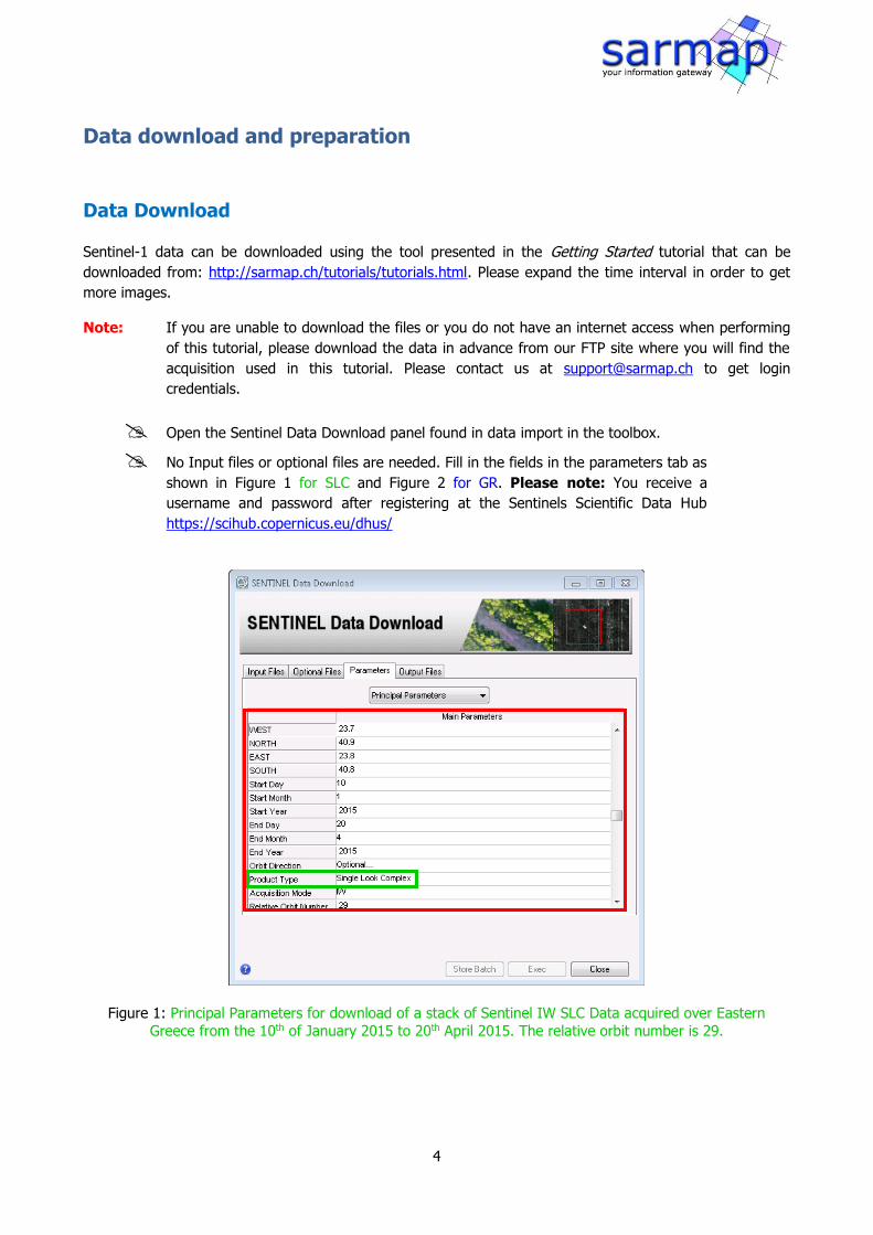
Open the Sentinel Data Download panel found in data import in the toolbox.

No Input files or optional files are needed. Fill in the fields in the parameters tab as

shown in Figure 1 for SLC and Figure 2 for GR. Please note: You receive a

username and password after registering at the Sentinels Scientific Data Hub

https://scihub.copernicus.eu/dhus/

Figure 1: Principal Parameters for download of a stack of Sentinel IW SLC Data acquired over Eastern

Greece from the 10th of January 2015 to 20th April 2015. The relative orbit number is 29.

5

Figure 2: Principal Parameters for download of a stack of Sentinel IW GR Data acquired over Eastern Greece

from the 10th of January 2015 to 20th April 2015. The relative orbit number is 29.

Choose a convenient output directory for the progress file. The downloaded data

will be saved in the same directory. Please note: make sure you have enough

available free disk space in this folder. SLC dataset needs 65 GB, GR dataset needs

14 GB of space. Space needed for zip extraction and processing is not taken into

account.

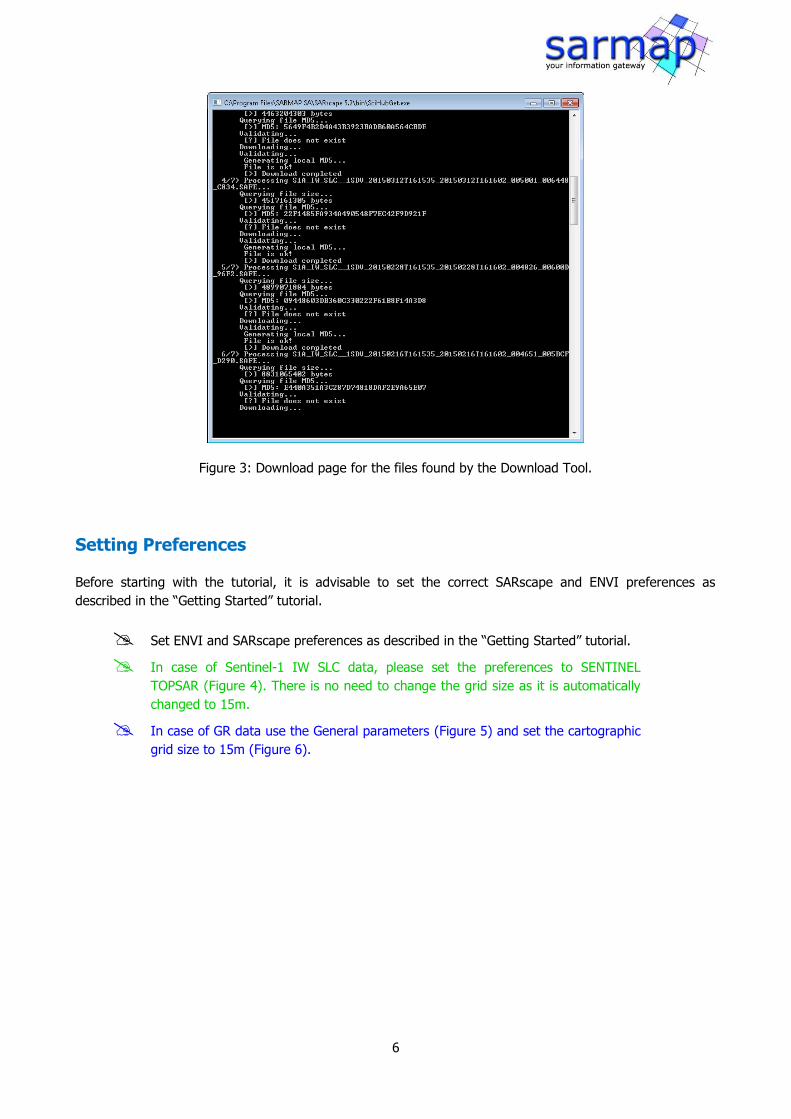
Click Exec. The following window should appear (Figure 3). Please wait for the

download to complete before continuing with the tutorial. During this time it is

possible to use ENVI or SARscape and it is even possible to close ENVI. The

window of Figure 3 will remain open.

6

Figure 3: Download page for the files found by the Download Tool.

Setting Preferences

Before starting with the tutorial, it is advisable to set the correct SARscape and ENVI preferences as

described in the “Getting Started” tutorial.

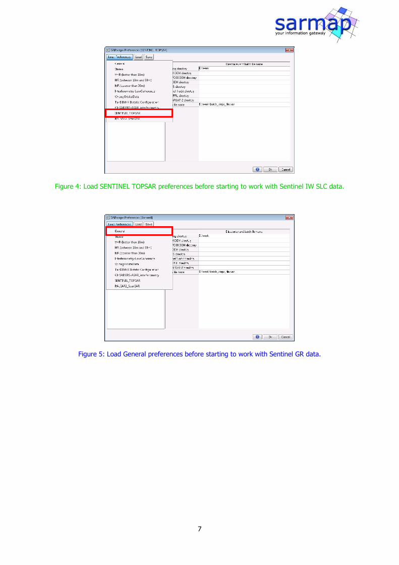
Set ENVI and SARscape preferences as described in the “Getting Started” tutorial.

In case of Sentinel-1 IW SLC data, please set the preferences to SENTINEL

TOPSAR (Figure 4). There is no need to change the grid size as it is automatically

changed to 15m.

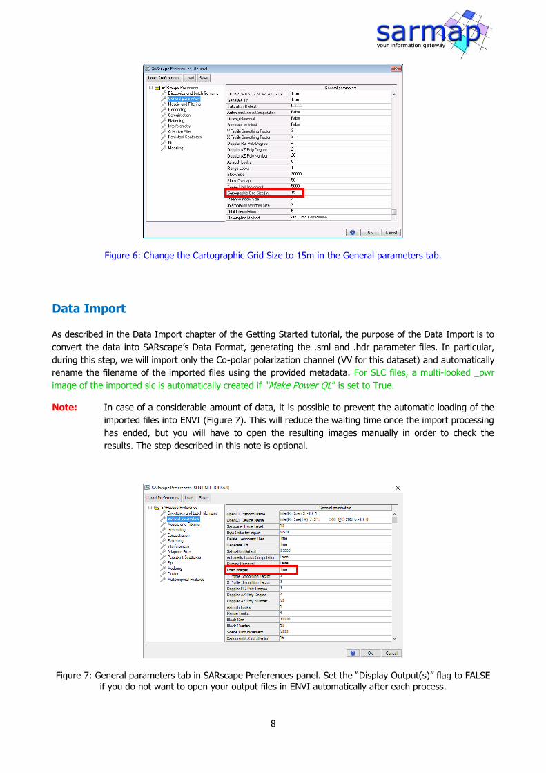
In case of GR data use the General parameters (Figure 5) and set the cartographic

grid size to 15m (Figure 6).

7

Figure 4: Load SENTINEL TOPSAR preferences before starting to work with Sentinel IW SLC data.

Figure 5: Load General preferences before starting to work with Sentinel GR data.

8

Figure 6: Change the Cartographic Grid Size to 15m in the General parameters tab.

Data Import

As described in the Data Import chapter of the Getting Started tutorial, the purpose of the Data Import is to

convert the data into SARscape’s Data Format, generating the .sml and .hdr parameter files. In particular,

during this step, we will import only the Co-polar polarization channel (VV for this dataset) and automatically

rename the filename of the imported files using the provided metadata. For SLC files, a multi-looked _pwr

image of the imported slc is automatically created if “Make Power QL” is set to True.

Note: In case of a considerable amount of data, it is possible to prevent the automatic loading of the

imported files into ENVI (Figure 7). This will reduce the waiting time once the import processing

has ended, but you will have to open the resulting images manually in order to check the

results. The step described in this note is optional.

Figure 7: General parameters tab in SARscape Preferences panel. Set the “Display Output(s)” flag to FALSE

if you do not want to open your output files in ENVI automatically after each process.

9

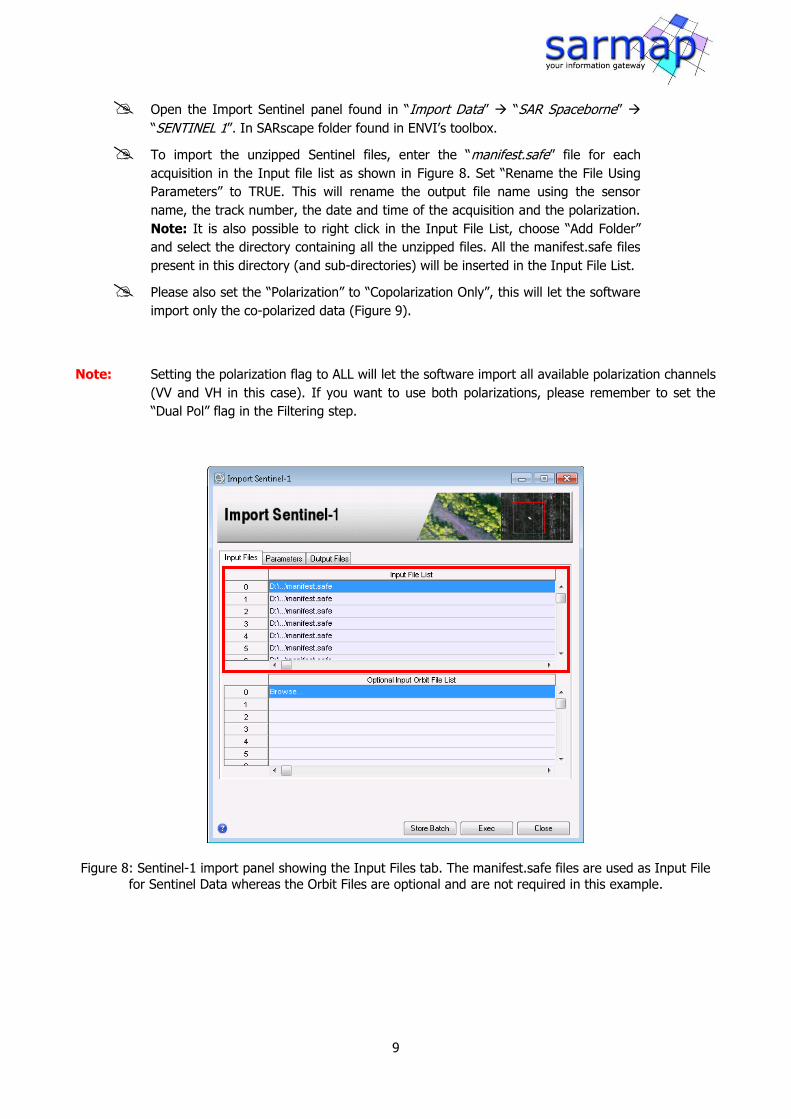
Open the Import Sentinel panel found in “Import Data” “SAR Spaceborne”

“SENTINEL 1”. In SARscape folder found in ENVI’s toolbox.

To import the unzipped Sentinel files, enter the “manifest.safe” file for each

acquisition in the Input file list as shown in Figure 8. Set “Rename the File Using

Parameters” to TRUE. This will rename the output file name using the sensor

name, the track number, the date and time of the acquisition and the polarization.

Note: It is also possible to right click in the Input File List, choose “Add Folder”

and select the directory containing all the unzipped files. All the manifest.safe files

present in this directory (and sub-directories) will be inserted in the Input File List.

Please also set the “Polarization” to “Copolarization Only”, this will let the software

import only the co-polarized data (Figure 9).

Note: Setting the polarization flag to ALL will let the software import all available polarization channels

(VV and VH in this case). If you want to use both polarizations, please remember to set the

“Dual Pol” flag in the Filtering step.

Figure 8: Sentinel-1 import panel showing the Input Files tab. The manifest.safe files are used as Input File

for Sentinel Data whereas the Orbit Files are optional and are not required in this example.

10

Figure 9: Principal parameters Tab of the Import Sentinel-1 panel. “Polarization” has to be set to

“Copolarization only” in order to import only copolarization data (VV for this dataset).

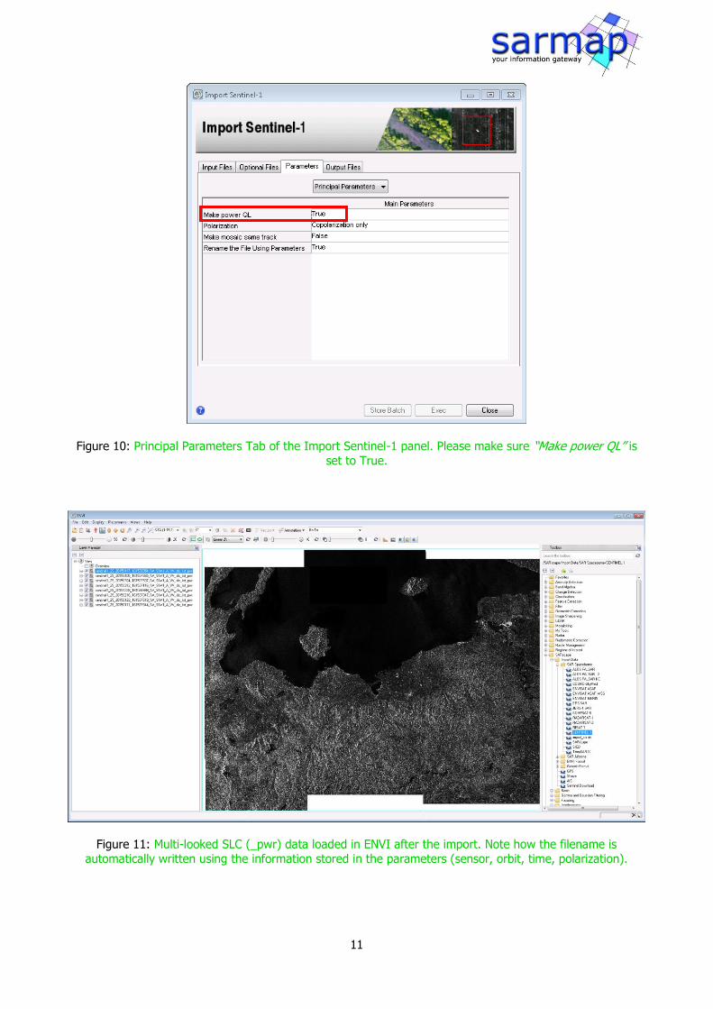
Make sure that in the Other Parameters “Make Power QL” is set to True (Figure

10). This will automatically create a multi-looked power image (_pwr) of the

imported slc. Right click on the Output File List and change the output directory to

a convenient one.

Click Exec. Once the import has ended, in the output folder you will find 8 _slc_list

files, 8 _pwr images and 8 folders, containing the _slc burst. The 8 _pwr are

automatically loaded in ENVI’s view (Figure 11).

Click Exec. Once the import has ended, in the output folder you will find 8 _gr file

(each one with his .hdr and .sml files), these files are automatically loaded in

ENVI’s view (Figure 12).

11

Figure 10: Principal Parameters Tab of the Import Sentinel-1 panel. Please make sure “Make power QL” is set to True.

Figure 11: Multi-looked SLC (_pwr) data loaded in ENVI after the import. Note how the filename is

automatically written using the information stored in the parameters (sensor, orbit, time, polarization).

12

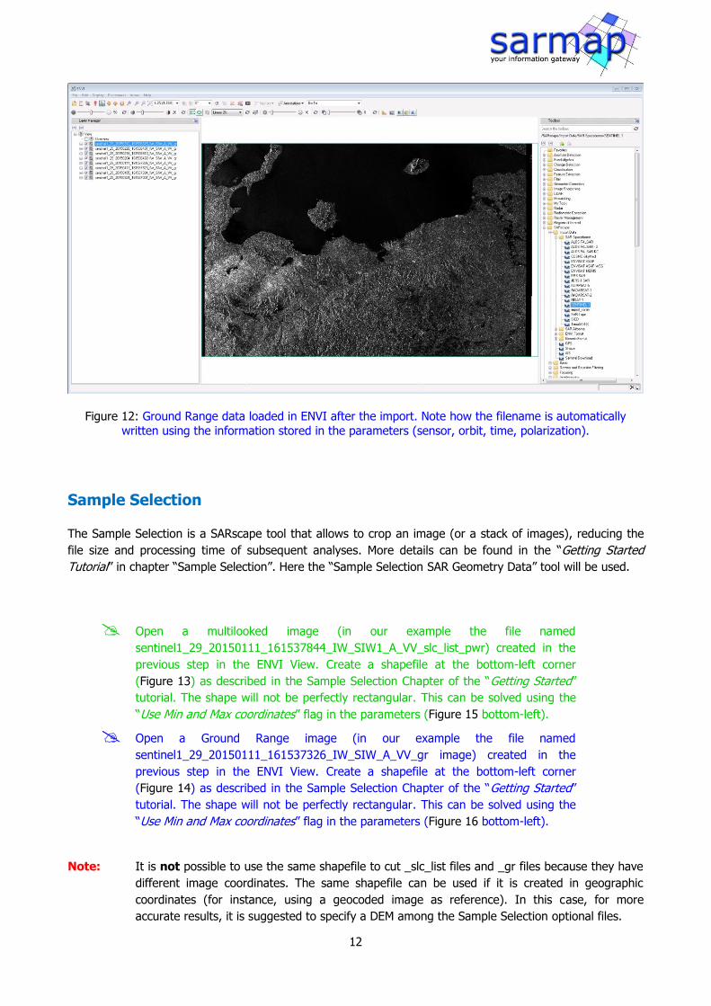
Figure 12: Ground Range data loaded in ENVI after the import. Note how the filename is automatically

written using the information stored in the parameters (sensor, orbit, time, polarization).

Sample Selection

The Sample Selection is a SARscape tool that allows to crop an image (or a stack of images), reducing the

file size and processing time of subsequent analyses. More details can be found in the “Getting Started

Tutorial” in chapter “Sample Selection”. Here the “Sample Selection SAR Geometry Data” tool will be used.

Open a multilooked image (in our example the file named

sentinel1_29_20150111_161537844_IW_SIW1_A_VV_slc_list_pwr) created in the

previous step in the ENVI View. Create a shapefile at the bottom-left corner

(Figure 13) as described in the Sample Selection Chapter of the “Getting Started”

tutorial. The shape will not be perfectly rectangular. This can be solved using the

“Use Min and Max coordinates” flag in the parameters (Figure 15 bottom-left).

Open a Ground Range image (in our example the file named

sentinel1_29_20150111_161537326_IW_SIW_A_VV_gr image) created in the

previous step in the ENVI View. Create a shapefile at the bottom-left corner

(Figure 14) as described in the Sample Selection Chapter of the “Getting Started”

tutorial. The shape will not be perfectly rectangular. This can be solved using the

“Use Min and Max coordinates” flag in the parameters (Figure 16 bottom-left).

Note: It is not possible to use the same shapefile to cut _slc_list files and _gr files because they have

different image coordinates. The same shapefile can be used if it is created in geographic

coordinates (for instance, using a geocoded image as reference). In this case, for more

accurate results, it is suggested to specify a DEM among the Sample Selection optional files.

13

Tip: Setting “Make coregistration” to TRUE, will reduce the risk of wrongly located cuts, which can

appear in case of shifted acquisition frames. This is however only a rough coregistration and

does not replace the coregistration step described in the dedicated chapter.

Figure 13: Polygon draw on sentinel1_29_20150111_161537844_IW_SIW1_A_VV_slc_list_pwr image. This is

the area of interest that will be used to cut SLC images.

14

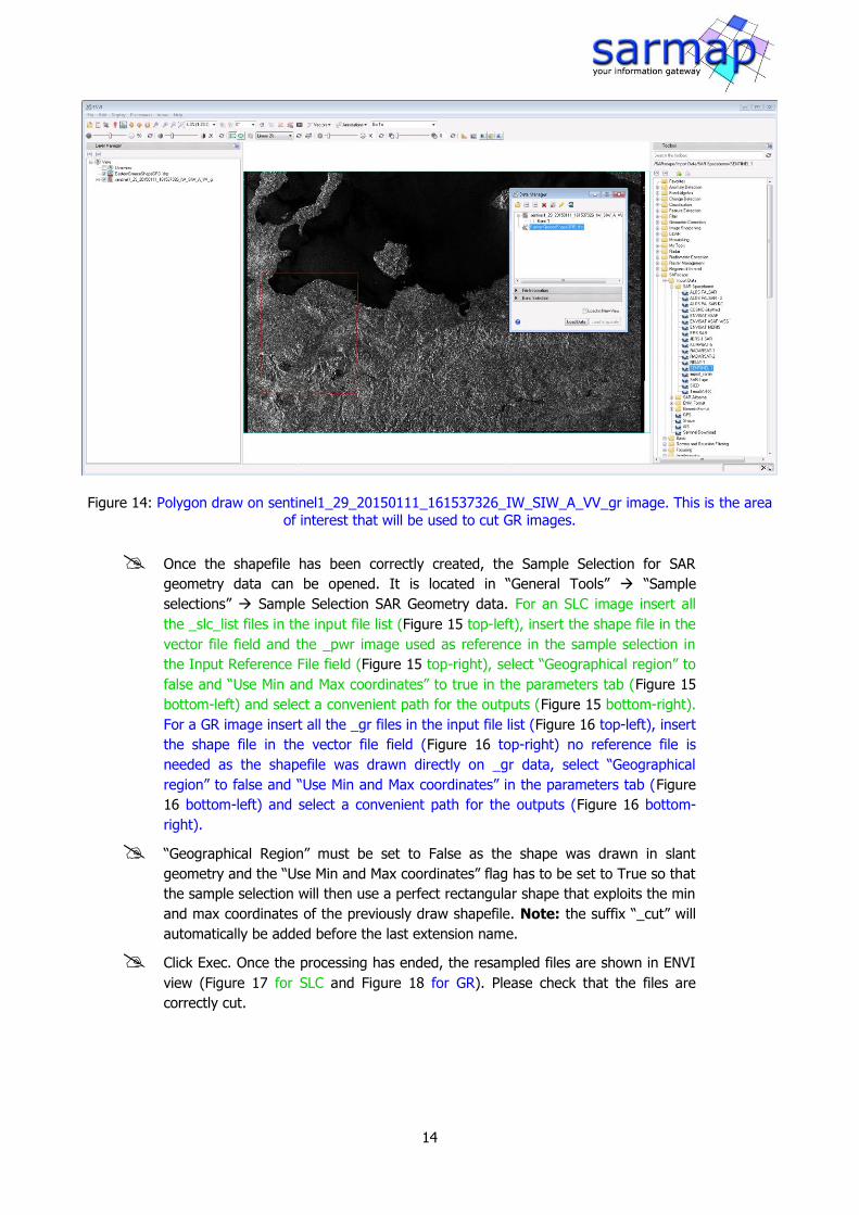
Figure 14: Polygon draw on sentinel1_29_20150111_161537326_IW_SIW_A_VV_gr image. This is the area

of interest that will be used to cut GR images.

Once the shapefile has been correctly created, the Sample Selection for SAR

geometry data can be opened. It is located in “General Tools” “Sample

selections” Sample Selection SAR Geometry data. For an SLC image insert all

the _slc_list files in the input file list (Figure 15 top-left), insert the shape file in the

vector file field and the _pwr image used as reference in the sample selection in

the Input Reference File field (Figure 15 top-right), select “Geographical region” to

false and “Use Min and Max coordinates” to true in the parameters tab (Figure 15

bottom-left) and select a convenient path for the outputs (Figure 15 bottom-right).

For a GR image insert all the _gr files in the input file list (Figure 16 top-left), insert

the shape file in the vector file field (Figure 16 top-right) no reference file is

needed as the shapefile was drawn directly on _gr data, select “Geographical

region” to false and “Use Min and Max coordinates” in the parameters tab (Figure

16 bottom-left) and select a convenient path for the outputs (Figure 16 bottom-

right).

“Geographical Region” must be set to False as the shape was drawn in slant

geometry and the “Use Min and Max coordinates” flag has to be set to True so that

the sample selection will then use a perfect rectangular shape that exploits the min

and max coordinates of the previously draw shapefile. Note: the suffix “_cut” will

automatically be added before the last extension name.

Click Exec. Once the processing has ended, the resampled files are shown in ENVI

view (Figure 17 for SLC and Figure 18 for GR). Please check that the files are

correctly cut.

15

Figure 15: Sample Selection SAR geometry Data panel. Top left: Input file list, insert here all the _slc_list files (not the _pwr). Top right: optional files tab, here the previously created shape file has to be entered as

well as the _pwr image used as a reference for drawing the shapefile. Bottom left: Parameters tab, set “Geographical region to False” (as the shapefile was drawn on an image in SAR geometry) and set “Use Min

and Max Coordinates” to True. Bottom right, output file list.

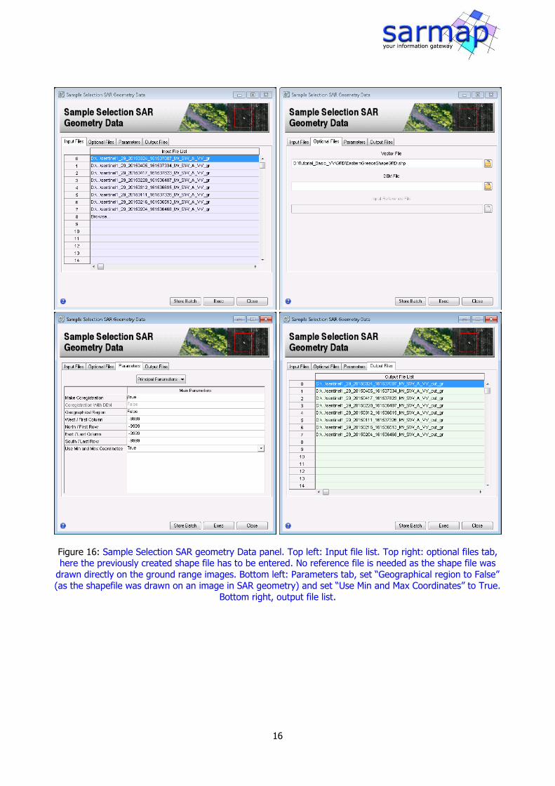
16

Figure 16: Sample Selection SAR geometry Data panel. Top left: Input file list. Top right: optional files tab, here the previously created shape file has to be entered. No reference file is needed as the shape file was

drawn directly on the ground range images. Bottom left: Parameters tab, set “Geographical region to False” (as the shapefile was drawn on an image in SAR geometry) and set “Use Min and Max Coordinates” to True.

Bottom right, output file list.

17

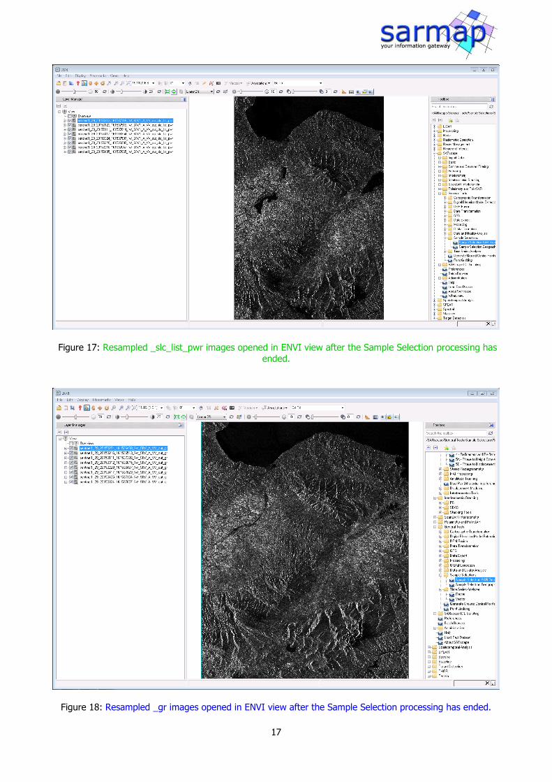
Figure 17: Resampled _slc_list_pwr images opened in ENVI view after the Sample Selection processing has

ended.

Figure 18: Resampled _gr images opened in ENVI view after the Sample Selection processing has ended.

18

Single Panels processing

This chapter shows the main tools of the SARscape Basic module performed step by step using the panels

present in the toolbox.

Coregistration

Coregistration is required when multiple images cover the same region and a time-series of pixel values

needs to be analyzed (e.g. for multi-temporal speckle filtering) or two images need to be compared, e.g.

through, image ratio or similar operations. Coregistration is simply the process of resampling an image in

slant- or ground-range coordinates to a reference acquisition geometry, also in slant- or ground-range

coordinates. This process must not to be confused with geocoding, which is the process of resampling each

pixel from slant- or ground-range coordinates to a cartographic reference system.

Note: If no DEM is inserted in the optional files, the coregistration with DEM will be discarded.

Open the Coregistration panel, found in “Basic” “Intensity Processing”

“Coregistration” and insert the _cut_pwr of the previously cut _slc_list (Figure 19

left) or the previously cut _cut_gr (Figure 20 left) in the “Input File List”. Insert the

first one as Reference File. The remaining images will be coregistered to (i.e.

resampled to the geometry of) the first one.

Choose a convenient output folder for the output files and click Exec (Figure 19

and Figure 20 right). There is no need to add optional files or to change the

parameters.

Figure 19: Coregistration Panel. Use the first image as a reference, the others will be coregistered to this

reference image.

19

Figure 20: Coregistration Panel. Use the first image as a reference, the others will be coregistered to this

reference image.

20

Filtering

Images obtained from coherent sensors such as SAR (or Laser) systems are characterized by speckle. This is

a spatially random multiplicative noise due to coherent superposition of multiple backscatter sources within a

SAR resolution element. In other words, speckle is a statistical fluctuation associated with the radar

reflectivity of each pixel in a scene. A first step to reduce the speckle - at the expense of spatial resolution -

is the so called multi-looking step, where range and/or azimuth resolution cells are averaged.

In our example, the De Grandi Spatio Temporal filtering will be used. It has to be pointed out that this multi-

temporal filtering is based on the assumption that the same resolution element on the ground is illuminated

by the radar beam in the same way, and corresponds to the same co-ordinates in the image plane in all

images of the time series. The reflectivity can of course change from one time to the next due to a change

in the dielectric and geometrical properties of the elementary scatters, but should not change due to a

different position of the resolution element with respect to the radar. Therefore it is mandatory to co-register

the SAR images in the time series to a common reference acquisition, before performing this kind of filtering.

Input data must be in radar geometry; geocoded (_geo) data are not admitted.

The filter works in a combined time-space domain. Each element in homogeneous areas with developed

speckle is averaged with corresponding uncorrelated elements in the time-series. The mean values of the

probability distribution function of each instance in the averaged series is adjusted to keep track of changes

in reflectivity. The adjustment is performed in space by estimation in a diagonal wavelet basis of the local

mean backscatter values in each data set. Since the wavelet based estimator preserves structures in the

image (such as edges and point targets), these structures (and changes thereof) are also preserved (and

denoised) by the time domain averaging (Figure 24).

In the DualPol case, the number of channels used in the LMMSE filtering will be doubled with respect to the

Single Pol version since both polarizations for each date will be used.

Note: It is suggested to always work with only one polarization type at once. It is however still

possible to perform DualPol De Grandi filtering: the order of the files should be “co-pol”

followed by “cross-pol” and the Data Type has to be set to “Dual pol”.

Figure 21: Unfiltered intensity image (left) and filtered intensity image (right) using the De Grandi filter. Note

how the filtered image is less noisy but preserves (and enhance) the linear features

21

Open the De Grandi Spatio Temporal Filtering panel, found in “Basic” “Intensity

Processing” “Filtering” “De Grandi Spatio Temporal Filtering” and insert the

previously coregistered _rsp data (_cut_pwr_rsp or _cut_gr_rsp) in the “Input File

List”. (Figure 22 for data coming from SLC and Figure 24 for data coming from

GR). Note: Use only VV polarized data.

Leave all the preferences as default. Check the datatype is set to “Single Pol” in

the Principal Parameters, choose a convenient output folder and click Exec. The

filtered results will be loaded automatically when the process ends (Figure 24 or

Figure 25).

Figure 22: Input files for De Grandi Spatio-Temporal Filter for data coming from IW SLC data. Note: data

type has to be set to “Single pol” as only VV files are involved in this tutorial.

22

Figure 23: Input files for De Grandi Spatio-Temporal Filter. Note: data type has to be set to “Single pol” as

only VV files are involved in this tutorial.

23

Figure 24: Filtered pwr images opened after the De Grandi filtering Process.

Figure 25: Filtered gr images opened after the De Grandi filtering Process.

24

Geocoding

SAR systems measure the ratio between the power of the pulse transmitted and that of the echo received.

This ratio (so-called backscatter) is projected into the slant range geometry. Geometric and radiometric

calibration of the backscatter values are necessary for inter-comparison of radar images acquired with

different sensors, or even of images obtained by the same sensor if acquired in different modes or

processed with different processors. Further information can be found in the Geocoding chapter of the

“Getting started” tutorial.

Open the Geocoding panel, found in “Basic” “Intensity Processing”

“Geocoding” “Geocoding and Radiometric Calibration” and insert the previously

filtered _pwr_rsp_fil or _gr_rsp_fil data in the “Input File List” (Figure 26 or Figure

27 top-left corner).

In the DEM/Cartographic System tab (Figure 26 or Figure 27 top-right corner) you

can either insert the DEM extracted for the “Getting Started Tutorial” or use the

binocular button to call the DEM extractor tool (Figure 28). When the DEM is

downloaded, the DEM extractor tool will automatically close and the path of the

DEM will appear in the correct field in the Geocoding Panel.

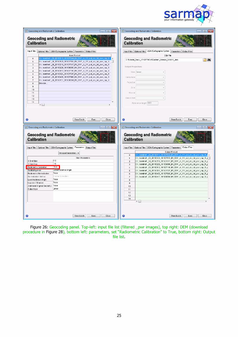
Check that the X and Y Gridsize is set to 15m and the Radiometric Calibration to

True in the preferences (Figure 26 or Figure 27 bottom-left corner) and set the

output file list to a convenient directory (Figure 26 or Figure 27 bottom-right

corner). Note: the suffix “_geo” will automatically be added after the last

extension name.

Click Exec. The geocoded images will be loaded at the end of the processing.

25

Figure 26: Geocoding panel. Top-left: input file list (filtered _pwr images), top right: DEM (download procedure in Figure 28), bottom left: parameters, set “Radiometric Calibration” to True, bottom right: Output

file list.

26

Figure 27: Geocoding panel. Top-left: input file list (filtered _gr images), top right: DEM (download procedure in Figure 28), bottom left: parameters, set “Radiometric Calibration” to True, bottom right: Output

file list.

27

Figure 28: Geocoding and Radiometric Calibration, DEM/Cartographic System tab. Use the binocular button

to call automatically the DEM extractor tool.

28

Feature Extraction – Multi Temporal features

Single-date and multi-temporal features, based on first order statistics, can be derived from SAR intensity

data. Depending on the targeted product, These features enable to detect and extract structures or

temporal changes, which can be additionally used for segmentation and/or classification purposes. A

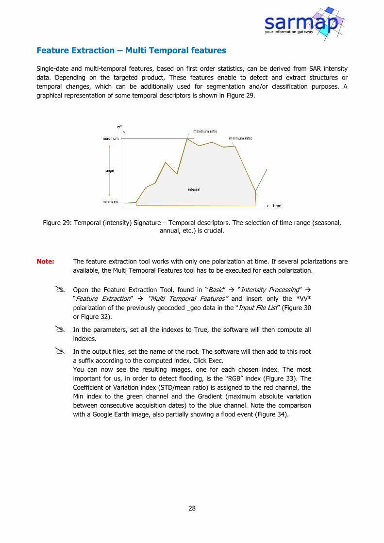
graphical representation of some temporal descriptors is shown in Figure 29.

Figure 29: Temporal (intensity) Signature – Temporal descriptors. The selection of time range (seasonal,

annual, etc.) is crucial.

Note: The feature extraction tool works with only one polarization at time. If several polarizations are

available, the Multi Temporal Features tool has to be executed for each polarization.

Open the Feature Extraction Tool, found in “Basic” “Intensity Processing”

“Feature Extraction” “Multi Temporal Features” and insert only the *VV*

polarization of the previously geocoded _geo data in the “Input File List” (Figure 30

or Figure 32).

In the parameters, set all the indexes to True, the software will then compute all

indexes.

In the output files, set the name of the root. The software will then add to this root

a suffix according to the computed index. Click Exec.

You can now see the resulting images, one for each chosen index. The most

important for us, in order to detect flooding, is the “RGB” index (Figure 33). The

Coefficient of Variation index (STD/mean ratio) is assigned to the red channel, the

Min index to the green channel and the Gradient (maximum absolute variation

between consecutive acquisition dates) to the blue channel. Note the comparison

with a Google Earth image, also partially showing a flood event (Figure 34).

29

Figure 30: Multi Temporal Features panel for filtered multilooked SLC data in VV polarization.

Figure 31: Multi Temporal Features panel, parameters Tab. Set all the features to True.

30

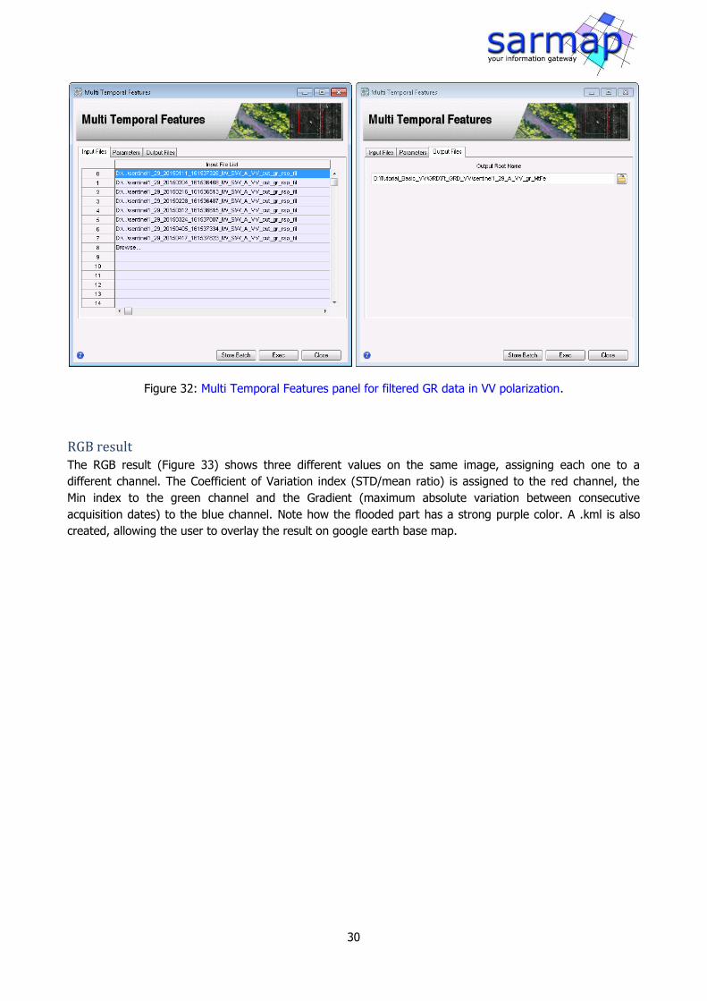
Figure 32: Multi Temporal Features panel for filtered GR data in VV polarization.

RGB result The RGB result (Figure 33) shows three different values on the same image, assigning each one to a

different channel. The Coefficient of Variation index (STD/mean ratio) is assigned to the red channel, the

Min index to the green channel and the Gradient (maximum absolute variation between consecutive

acquisition dates) to the blue channel. Note how the flooded part has a strong purple color. A .kml is also

created, allowing the user to overlay the result on google earth base map.

31

Figure 33: “RGB” result of the “Feature extraction tool. Note in the selected area the dark zone that refers to

a low backscatter zone, caused by an overflowed river that flooded the floodplain.

Figure 34: Comparison of the floodplain on the “RGB” result and google earth image. Left part of the Google

Earth image was acquired on the 10th of April 2015 and the right part on the 18th of March 2014. Note how

the flooded image in google earth matches the dark area in the “Min” result.

Multitemporal features The other multitemporal features are located in the same output folder. In addition, a _meta file is created.

This file contains all temporal descriptors selected in Figure 31 as well as all filtered geocoded images. This

will show up in the ENVI Data manager as follows (Figure 35).

10.04.2015 18.03.2014

32

This particular file type allows the user to create RGB images “on the fly” by simply clicking on the white

square at the left side of the image name to assign the band and the “load data” button at the bottom as

described in Figure 35. This can be done using the single filtered geocoded images as in Figure 36 as well as

using the temporal descriptors (Figure 37).

Figure 35: ENVI Data manager containing the _meta created in the Multi Temporal Features step. It shows

all filtered geocoded acquisitions in the upper part and the temporal descriptors in the lower part.

33

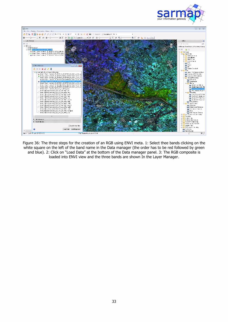
Figure 36: The three steps for the creation of an RGB using ENVI meta. 1: Select thee bands clicking on the

white square on the left of the band name in the Data manager (the order has to be red followed by green

and blue). 2: Click on “Load Data” at the bottom of the Data manager panel. 3: The RGB composite is

loaded into ENVI view and the three bands are shown In the Layer Manager.

34

Figure 37: Another example of the three steps for the creation of an RGB using ENVI meta as in Figure 36 but using the temporal descriptors instead of the single acquisitions. This example uses the Minimum in the

red channel, the Minimum ratio in the green channel and the Span Ratio in the blue channel.

Otherwise, if more complex RGB image have to be created, it is possible to use the SARscape tool found in

“SARscape > General Tools > Data Export > Generate Color Composite”. This tool allows to perform several

different types of RGB operations and to adapt the scale, exponent and other parameters for each channel.

Please refer to the Help for more information.

35

Workflow

This chapter will show how to use SARscape workflows in the Basic module. The first sub-chapter will

concentrate on replicating the process performed in the Single Panels chapter using the Intensity Time

Series Workflow and using the “next” buttons (which will cause a pause after each step). The second sub-

section will show a usage example of the Coherence RGB workflow. In this case, the “Next >>>” button is

used, which allows to perform all the steps with only one click. The operation of a SARscape workflow is

explained in the Getting Started tutorial that can be downloaded from here:

http://sarmap.ch/tutorials/tutorials.html.

Note: During the execution of workflows, it is not allowed to close the window or launch other

processes.

Intensity time series workflow

For this tutorial, Sentinel-1 data will be used. The data can be downloaded using the tool presented in the

Data Download section at page 4 of this tutorial. In this example, we will use only the resampled SLC files

(_cut_slc_list) in VV polarization. This workflow can be performed with ground range too.

This workflow is found in SARscape>Basic>Intensity Time Series Workflow.

Tip: Use the resampled data as input in order to perform the workflow only on the area of interest

defined in the Sample Selection chapter.

Note: With the workflow, it is not possible to ingest dual-pol data, as they have to be used separately

for the multi temporal features analysis.

Open the Intensity Time Series Workflow found in “Basic” and fill in the

_cut_slc_list files in VV polarization (they have to be previously imported and

resampled in SARscape as described in the relative section in the Data download

and preparation chapter) as shown in Figure 38. Set up the DEM/Cartographic

System tab as described in Figure 39 in order to automatically download an

SRTM3v4 DEM and then set the gridsize to 15m (Figure 40).

Click “Next >” This button allows to start downloading the DEM and then jump to

the next step. Note: You will be asked to confirm the look-factor once the

workflow has finished with the DEM download.

36

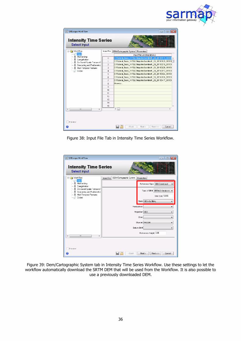
Figure 38: Input File Tab in Intensity Time Series Workflow.

Figure 39: Dem/Cartographic System tab in Intensity Time Series Workflow. Use these settings to let the

workflow automatically download the SRTM DEM that will be used from the Workflow. It is also possible to

use a previously downloaded DEM.

37

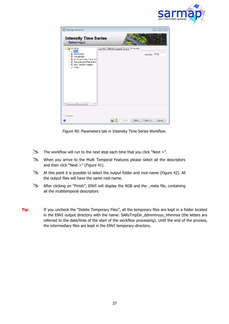
Figure 40: Parameters tab in Intensity Time Series Workflow.

The workflow will run to the next step each time that you click “Next >”.

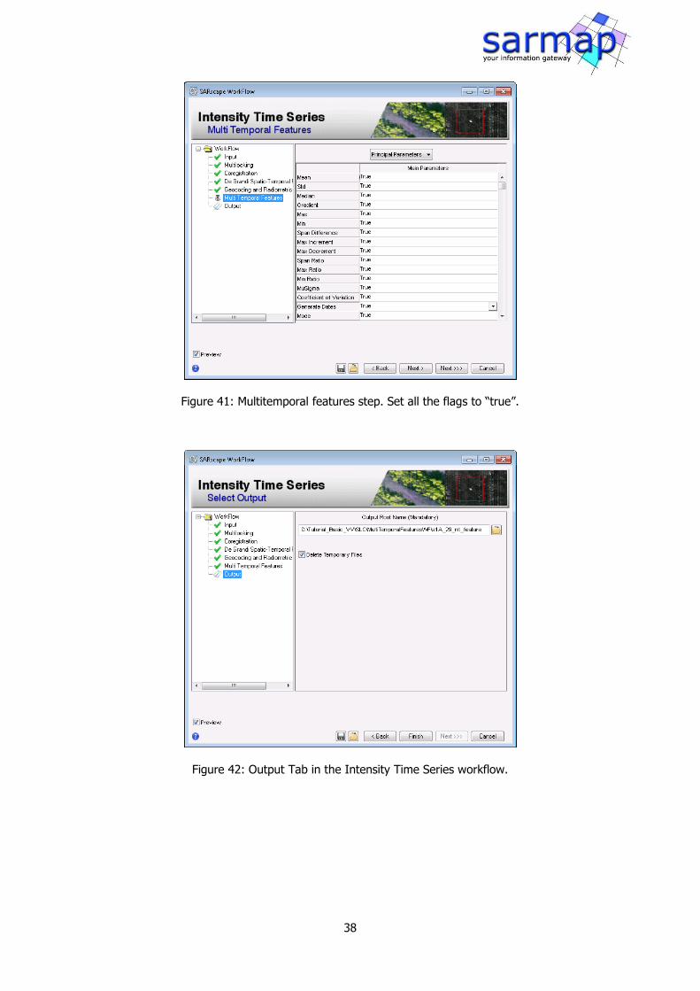
When you arrive to the Multi Temporal Features please select all the descriptors

and then click “Next >” (Figure 41).

At this point it is possible to select the output folder and root-name (Figure 42). All

the output files will have the same root-name.

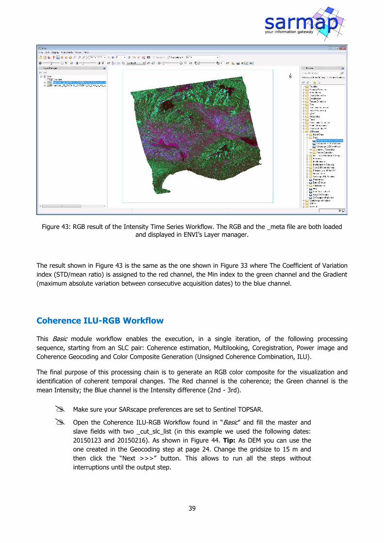
After clicking on “Finish”, ENVI will display the RGB and the _meta file, containing

all the multitemporal descriptors

Tip: If you uncheck the “Delete Temporary Files”, all the temporary files are kept in a folder located

in the ENVI output directory with the name: SARsTmpDir_ddmmmyyy_hhmmss (the letters are

referred to the date/time of the start of the workflow processing). Until the end of the process,

the intermediary files are kept in the ENVI temporary directory.

38

Figure 41: Multitemporal features step. Set all the flags to “true”.

Figure 42: Output Tab in the Intensity Time Series workflow.

39

Figure 43: RGB result of the Intensity Time Series Workflow. The RGB and the _meta file are both loaded

and displayed in ENVI’s Layer manager.

The result shown in Figure 43 is the same as the one shown in Figure 33 where The Coefficient of Variation

index (STD/mean ratio) is assigned to the red channel, the Min index to the green channel and the Gradient

(maximum absolute variation between consecutive acquisition dates) to the blue channel.

Coherence ILU-RGB Workflow

This Basic module workflow enables the execution, in a single iteration, of the following processing

sequence, starting from an SLC pair: Coherence estimation, Multilooking, Coregistration, Power image and

Coherence Geocoding and Color Composite Generation (Unsigned Coherence Combination, ILU).

The final purpose of this processing chain is to generate an RGB color composite for the visualization and

identification of coherent temporal changes. The Red channel is the coherence; the Green channel is the

mean Intensity; the Blue channel is the Intensity difference (2nd - 3rd).

Make sure your SARscape preferences are set to Sentinel TOPSAR.

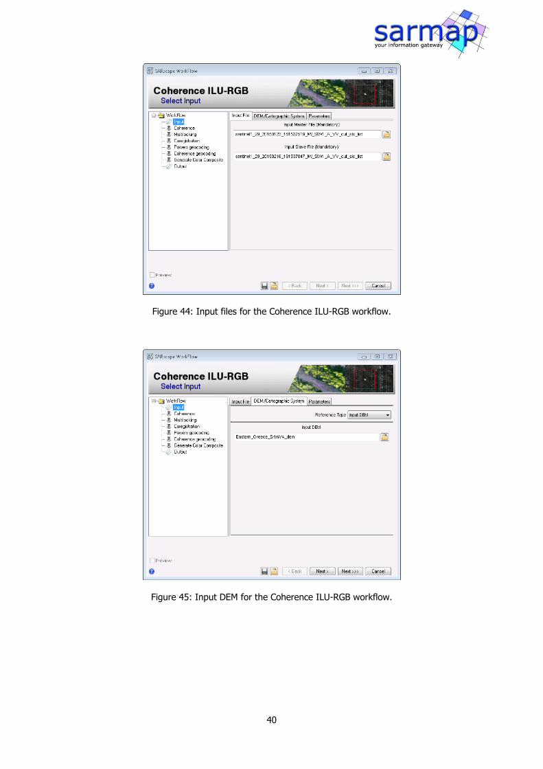
Open the Coherence ILU-RGB Workflow found in “Basic” and fill the master and

slave fields with two _cut_slc_list (in this example we used the following dates:

20150123 and 20150216). As shown in Figure 44. Tip: As DEM you can use the

one created in the Geocoding step at page 24. Change the gridsize to 15 m and

then click the “Next >>>” button. This allows to run all the steps without

interruptions until the output step.

40

Figure 44: Input files for the Coherence ILU-RGB workflow.

Figure 45: Input DEM for the Coherence ILU-RGB workflow.

41

Figure 46: Parameters Tab. Check that the Grid Size is set to 15 m.

The software will then start to process all the steps one after another without interruptions until the output

tab appears (Figure 47). As a result, an Unsigned Coherence Combination RGB color composite is shown in

ENVI (Figure 48) as well as the geocoded multilooked master and slave acquisition and the geocoded

coherence.

Figure 47: All the steps of the workflow are performed in a row when the “Next >>>” button is used.

42

Figure 48: ILU RGB tiff result shown in ENVI. The Red channel is the coherence; the Green channel is the

mean Intensity; the Blue channel is the Intensity difference (2nd - 3rd).