Embed Size (px)
Citation preview

SAP2000®
IntegratedFinite Element Analysis
andDesign of Structures
ANALYSIS REFERENCE
COMPUTERS &
STRUCTURES
INC.
Computers and Structures, Inc.Berkeley, California, USA
Version 7.0Revised October 1998
1

COPYRIGHT
The computer program SAP2000 and all associated documentation areproprietary and copyrighted products. Worldwide rights of ownershiprest with Computers and Structures, Inc. Unlicensed use of the programor reproduction of the documentation in any form, without prior writtenauthorization from Computers and Structures, Inc., is explicitly prohib-ited.
Further information and copies of this documentation may be obtainedfrom:
Computers and Structures, Inc.1995 University Avenue
Berkeley, California 94704 USA
tel: (510) 845-2177fax: (510) 845-4096
e-mail: [email protected]:www.csiberkeley.com
© Copyright Computers and Structures, Inc., 1978–1998.The CSI Logo is a registered trademark of Computers and Structures, Inc.SAP2000 is a registered trademark of Computers and Structures, Inc.Windows is a registered trademark of Microsoft Corporation.
2

DISCLAIMER
CONSIDERABLE TIME, EFFORT AND EXPENSE HAVE GONEINTO THE DEVELOPMENT AND DOCUMENTATION OFSAP2000. THE PROGRAM HAS BEEN THOROUGHLY TESTEDAND USED. IN USING THE PROGRAM, HOWEVER, THE USERACCEPTS AND UNDERSTANDS THAT NO WARRANTY IS EX-PRESSED OR IMPLIED BY THE DEVELOPERS OR THE DIS-TRIBUTORS ON THE ACCURACY OR THE RELIABILITY OFTHE PROGRAM.
THE USER MUST EXPLICITLY UNDERSTAND THE ASSUMP-TIONS OF THE PROGRAM AND MUST INDEPENDENTLY VER-IFY THE RESULTS.
3

ACKNOWLEDGMENT
Thanks are due to all of the numerous structural engineers, who over theyears have given valuable feedback that has contributed toward the en-hancement of this product to its current state.
Special recognition is due Dr. Edward L. Wilson, Professor Emeritus,University of California at Berkeley, who was responsible for the con-ception and development of the original SAP series of programs andwhose continued originality has produced many unique concepts thathave been implemented in this version.
4

Table of Contents
Chapter I Introduction 1
SAP2000 Analysis Features . . . . . . . . . . . . . . . . . . . . . . . 1
Structural Analysis and Design . . . . . . . . . . . . . . . . . . . . . . 2
About This Manual . . . . . . . . . . . . . . . . . . . . . . . . . . . . 3
Topics . . . . . . . . . . . . . . . . . . . . . . . . . . . . . . . . . . . 3
Typographical Conventions. . . . . . . . . . . . . . . . . . . . . . . . 4
Bold for Definitions . . . . . . . . . . . . . . . . . . . . . . . . . 4Bold for Variable Data . . . . . . . . . . . . . . . . . . . . . . . . 4Italics for Mathematical Variables . . . . . . . . . . . . . . . . . . 4Italics for Emphasis . . . . . . . . . . . . . . . . . . . . . . . . . 4All Capitals for Literal Data . . . . . . . . . . . . . . . . . . . . . 5Capitalized Names . . . . . . . . . . . . . . . . . . . . . . . . . . 5
Bibliographic References . . . . . . . . . . . . . . . . . . . . . . . . . 5
Chapter II Labels, Arrays, and Generation 7
Overview . . . . . . . . . . . . . . . . . . . . . . . . . . . . . . . . . 8
Labels . . . . . . . . . . . . . . . . . . . . . . . . . . . . . . . . . . . 8
Label Increments . . . . . . . . . . . . . . . . . . . . . . . . . . . . . 9
Regular Arrays. . . . . . . . . . . . . . . . . . . . . . . . . . . . . . 10
Single Label. . . . . . . . . . . . . . . . . . . . . . . . . . . . . 11One-dimensional Regular Arrays . . . . . . . . . . . . . . . . . . 11Two-dimensional Regular Arrays . . . . . . . . . . . . . . . . . 12Three-dimensional Regular Arrays . . . . . . . . . . . . . . . . . 13
Generation . . . . . . . . . . . . . . . . . . . . . . . . . . . . . . . . 14
Joints . . . . . . . . . . . . . . . . . . . . . . . . . . . . . . . . 14Elements, Constraints, and Welds . . . . . . . . . . . . . . . . . 15
i
5

Deletion . . . . . . . . . . . . . . . . . . . . . . . . . . . . . . . . . 18
Assignment . . . . . . . . . . . . . . . . . . . . . . . . . . . . . . . 19
Chapter III Coordinate Systems 21
Overview. . . . . . . . . . . . . . . . . . . . . . . . . . . . . . . . . 22
Global Coordinate System. . . . . . . . . . . . . . . . . . . . . . . . 22
Upward and Horizontal Directions . . . . . . . . . . . . . . . . . . . 23
Defining Coordinate Systems . . . . . . . . . . . . . . . . . . . . . . 23
Vector Cross Product . . . . . . . . . . . . . . . . . . . . . . . . 23Defining the Three Axes Using Two Vectors . . . . . . . . . . . 24
Local Coordinate Systems . . . . . . . . . . . . . . . . . . . . . . . . 24
Alternate Coordinate Systems . . . . . . . . . . . . . . . . . . . . . . 26
Cylindrical and Spherical Coordinates . . . . . . . . . . . . . . . . . 28
Chapter IV Joint Coordinates 31
Overview. . . . . . . . . . . . . . . . . . . . . . . . . . . . . . . . . 32
Joint Definition . . . . . . . . . . . . . . . . . . . . . . . . . . . . . 32
One-dimensional Joint Generation . . . . . . . . . . . . . . . . . . . 33
One-dimensional Joint Array Specification . . . . . . . . . . . . 33One-dimensional Joint Definition . . . . . . . . . . . . . . . . . 33One-dimensional Linear Generation . . . . . . . . . . . . . . . . 34One-dimensional Cylindrical Generation. . . . . . . . . . . . . . 34
Two-dimensional Joint Generation . . . . . . . . . . . . . . . . . . . 36
Two-dimensional Joint Array Specification . . . . . . . . . . . . 37Two-dimensional Joint Definition . . . . . . . . . . . . . . . . . 37Two-dimensional Linear Generation . . . . . . . . . . . . . . . . 38Two-dimensional Frontal Generation. . . . . . . . . . . . . . . . 38Two-dimensional Edge Generation. . . . . . . . . . . . . . . . . 40
Three-dimensional Joint Generation. . . . . . . . . . . . . . . . . . . 43
Three-dimensional Joint Array Specification. . . . . . . . . . . . 43Three-dimensional Joint Definition. . . . . . . . . . . . . . . . . 44Three-dimensional Linear Generation . . . . . . . . . . . . . . . 45Three-dimensional Frontal Generation . . . . . . . . . . . . . . . 46Three-dimensional Edge Generation . . . . . . . . . . . . . . . . 46
Variable Joint Spacing. . . . . . . . . . . . . . . . . . . . . . . . . . 47
One Dimension . . . . . . . . . . . . . . . . . . . . . . . . . . . 48Two Dimensions . . . . . . . . . . . . . . . . . . . . . . . . . . 48Three Dimensions. . . . . . . . . . . . . . . . . . . . . . . . . . 49
Joint Definition in Polar Coordinates . . . . . . . . . . . . . . . . . . 50
Cylindrical Coordinates. . . . . . . . . . . . . . . . . . . . . . . 50
ii
SAP2000 Analysis Reference
6

Spherical Coordinates. . . . . . . . . . . . . . . . . . . . . . . . 52Variable Joint Spacing in Polar Coordinates . . . . . . . . . . . . 53
Joint Definition in Alternate Coordinate Systems. . . . . . . . . . . . 54
Chapter V Joint Patterns 57
Overview. . . . . . . . . . . . . . . . . . . . . . . . . . . . . . . . . 58
Pattern Definition . . . . . . . . . . . . . . . . . . . . . . . . . . . . 59
Gradient or Hydrostatic Specification . . . . . . . . . . . . . . . . . . 59
One-dimensional Pattern-value Generation . . . . . . . . . . . . . . . 60
Joint Array Specification . . . . . . . . . . . . . . . . . . . . . . 61One-dimensional Addition . . . . . . . . . . . . . . . . . . . . . 62One-dimensional Gradient Addition . . . . . . . . . . . . . . . . 62One-dimensional Linear Mapping . . . . . . . . . . . . . . . . . 63
Two-dimensional Pattern-value Generation . . . . . . . . . . . . . . . 63
Joint Array Specification . . . . . . . . . . . . . . . . . . . . . . 64Two-dimensional Addition . . . . . . . . . . . . . . . . . . . . . 64Two-dimensional Gradient Addition . . . . . . . . . . . . . . . . 65Two-dimensional Linear Mapping . . . . . . . . . . . . . . . . . 65Two-dimensional Frontal Mapping. . . . . . . . . . . . . . . . . 66Two-dimensional Edge Mapping . . . . . . . . . . . . . . . . . . 66
Three-dimensional Pattern-value Generation . . . . . . . . . . . . . . 67
Joint Array Specification . . . . . . . . . . . . . . . . . . . . . . 67Three-dimensional Addition . . . . . . . . . . . . . . . . . . . . 68Three-dimensional Gradient Addition . . . . . . . . . . . . . . . 69Three-dimensional Linear Mapping . . . . . . . . . . . . . . . . 69Three-dimensional Frontal Mapping . . . . . . . . . . . . . . . . 70Three-dimensional Edge Mapping . . . . . . . . . . . . . . . . . 71
Variable Pattern-value Increments . . . . . . . . . . . . . . . . . . . 72
One Dimension . . . . . . . . . . . . . . . . . . . . . . . . . . . 73Two Dimensions . . . . . . . . . . . . . . . . . . . . . . . . . . 73Three Dimensions. . . . . . . . . . . . . . . . . . . . . . . . . . 74
Chapter VI Joints and Degrees of Freedom 75
Overview. . . . . . . . . . . . . . . . . . . . . . . . . . . . . . . . . 76
Modeling Considerations . . . . . . . . . . . . . . . . . . . . . . . . 77
Local Coordinate System . . . . . . . . . . . . . . . . . . . . . . . . 78
Advanced Local Coordinate System . . . . . . . . . . . . . . . . . . 79
Reference Vectors . . . . . . . . . . . . . . . . . . . . . . . . . 79Defining the Axis Reference Vector . . . . . . . . . . . . . . . . 80Defining the Plane Reference Vector . . . . . . . . . . . . . . . . 80Determining the Local Axes from the Reference Vectors . . . . . 81
iii
Table of Contents
7

Joint Coordinate Angles . . . . . . . . . . . . . . . . . . . . . . 82
Degrees of Freedom . . . . . . . . . . . . . . . . . . . . . . . . . . . 83
Available and Unavailable Degrees of Freedom . . . . . . . . . . 85Restrained Degrees of Freedom . . . . . . . . . . . . . . . . . . 86Constrained Degrees of Freedom . . . . . . . . . . . . . . . . . . 86Active Degrees of Freedom. . . . . . . . . . . . . . . . . . . . . 86Null Degrees of Freedom . . . . . . . . . . . . . . . . . . . . . . 88
Restraints and Reactions. . . . . . . . . . . . . . . . . . . . . . . . . 88
Springs . . . . . . . . . . . . . . . . . . . . . . . . . . . . . . . . . . 89
Masses . . . . . . . . . . . . . . . . . . . . . . . . . . . . . . . . . . 91
Force Load. . . . . . . . . . . . . . . . . . . . . . . . . . . . . . . . 93
Restraint Displacement Load . . . . . . . . . . . . . . . . . . . . . . 93
Spring Displacement Load . . . . . . . . . . . . . . . . . . . . . . . 95
Degree of Freedom Output . . . . . . . . . . . . . . . . . . . . . . . 97
Joint Mass Output . . . . . . . . . . . . . . . . . . . . . . . . . . . . 98
Displacement and Acceleration Output . . . . . . . . . . . . . . . . 100
Force Output . . . . . . . . . . . . . . . . . . . . . . . . . . . . . . 102
Applied Loads . . . . . . . . . . . . . . . . . . . . . . . . . . . 103Inertial Loads . . . . . . . . . . . . . . . . . . . . . . . . . . . 104Stiffness Forces . . . . . . . . . . . . . . . . . . . . . . . . . . 106Spring Forces . . . . . . . . . . . . . . . . . . . . . . . . . . . 106Nllink Forces . . . . . . . . . . . . . . . . . . . . . . . . . . . 106Restraint Forces (Reactions). . . . . . . . . . . . . . . . . . . . 106Constraint Forces . . . . . . . . . . . . . . . . . . . . . . . . . 107P-Delta Moments . . . . . . . . . . . . . . . . . . . . . . . . . 107
Global Force Balance Output . . . . . . . . . . . . . . . . . . . . . 107
Chapter VII Constraints and Welds 113
Overview . . . . . . . . . . . . . . . . . . . . . . . . . . . . . . . . 114
Body Constraint . . . . . . . . . . . . . . . . . . . . . . . . . . . . 115
Joint Connectivity . . . . . . . . . . . . . . . . . . . . . . . . . 115Local Coordinate System . . . . . . . . . . . . . . . . . . . . . 115Constraint Equations . . . . . . . . . . . . . . . . . . . . . . . 115
Plane Definition . . . . . . . . . . . . . . . . . . . . . . . . . . . . 116
Diaphragm Constraint . . . . . . . . . . . . . . . . . . . . . . . . . 117
Joint Connectivity . . . . . . . . . . . . . . . . . . . . . . . . . 117Local Coordinate System . . . . . . . . . . . . . . . . . . . . . 117Constraint Equations . . . . . . . . . . . . . . . . . . . . . . . 118
Plate Constraint. . . . . . . . . . . . . . . . . . . . . . . . . . . . . 119
Joint Connectivity . . . . . . . . . . . . . . . . . . . . . . . . . 119Local Coordinate System . . . . . . . . . . . . . . . . . . . . . 119
iv
SAP2000 Analysis Reference
8

Constraint Equations . . . . . . . . . . . . . . . . . . . . . . . 119
Axis Definition . . . . . . . . . . . . . . . . . . . . . . . . . . . . . 120
Rod Constraint . . . . . . . . . . . . . . . . . . . . . . . . . . . . . 120
Joint Connectivity . . . . . . . . . . . . . . . . . . . . . . . . . 121Local Coordinate System . . . . . . . . . . . . . . . . . . . . . 122Constraint Equations . . . . . . . . . . . . . . . . . . . . . . . 122
Beam Constraint . . . . . . . . . . . . . . . . . . . . . . . . . . . . 122
Joint Connectivity . . . . . . . . . . . . . . . . . . . . . . . . . 123Local Coordinate System . . . . . . . . . . . . . . . . . . . . . 123Constraint Equations . . . . . . . . . . . . . . . . . . . . . . . 123
Equal Constraint . . . . . . . . . . . . . . . . . . . . . . . . . . . . 124
Joint Connectivity . . . . . . . . . . . . . . . . . . . . . . . . . 124Local Coordinate System . . . . . . . . . . . . . . . . . . . . . 125Selected Degrees of Freedom . . . . . . . . . . . . . . . . . . . 125Constraint Equations . . . . . . . . . . . . . . . . . . . . . . . 125
Local Constraint . . . . . . . . . . . . . . . . . . . . . . . . . . . . 127
Joint Connectivity . . . . . . . . . . . . . . . . . . . . . . . . . 127No Local Coordinate System . . . . . . . . . . . . . . . . . . . 128Selected Degrees of Freedom . . . . . . . . . . . . . . . . . . . 128Constraint Equations . . . . . . . . . . . . . . . . . . . . . . . 128
Welds . . . . . . . . . . . . . . . . . . . . . . . . . . . . . . . . . . 131
Automatic Master Joints . . . . . . . . . . . . . . . . . . . . . . . . 132
Stiffness, Mass, and Loads . . . . . . . . . . . . . . . . . . . . 132Local Coordinate Systems. . . . . . . . . . . . . . . . . . . . . 133
Constraint Output. . . . . . . . . . . . . . . . . . . . . . . . . . . . 133
Chapter VIII Material Properties 135
Overview . . . . . . . . . . . . . . . . . . . . . . . . . . . . . . . . 136
Local Coordinate System. . . . . . . . . . . . . . . . . . . . . . . . 136
Stresses and Strains. . . . . . . . . . . . . . . . . . . . . . . . . . . 137
Isotropic Materials . . . . . . . . . . . . . . . . . . . . . . . . . . . 138
Orthotropic Materials. . . . . . . . . . . . . . . . . . . . . . . . . . 139
Anisotropic Materials . . . . . . . . . . . . . . . . . . . . . . . . . 140
Temperature-Dependent Properties . . . . . . . . . . . . . . . . . . 141
Element Material Temperature . . . . . . . . . . . . . . . . . . . . . 142
Mass Density . . . . . . . . . . . . . . . . . . . . . . . . . . . . . . 142
Weight Density . . . . . . . . . . . . . . . . . . . . . . . . . . . . . 143
Design-Type Indicator . . . . . . . . . . . . . . . . . . . . . . . . . 143
v
Table of Contents
9

Chapter IX The Frame Element 145
Overview . . . . . . . . . . . . . . . . . . . . . . . . . . . . . . . . 146
Joint Connectivity . . . . . . . . . . . . . . . . . . . . . . . . . . . 147
Degrees of Freedom . . . . . . . . . . . . . . . . . . . . . . . . . . 147
Local Coordinate System. . . . . . . . . . . . . . . . . . . . . . . . 148
Longitudinal Axis 1 . . . . . . . . . . . . . . . . . . . . . . . . 148Default Orientation . . . . . . . . . . . . . . . . . . . . . . . . 148Coordinate Angle . . . . . . . . . . . . . . . . . . . . . . . . . 149
Advanced Local Coordinate System . . . . . . . . . . . . . . . . . . 149
Reference Vector . . . . . . . . . . . . . . . . . . . . . . . . . 150Determining Transverse Axes 2 and 3 . . . . . . . . . . . . . . 153
Section Properties . . . . . . . . . . . . . . . . . . . . . . . . . . . 153
Local Coordinate System . . . . . . . . . . . . . . . . . . . . . 154Material Properties . . . . . . . . . . . . . . . . . . . . . . . . 154Geometric Properties and Section Stiffnesses. . . . . . . . . . . 154Shape Type . . . . . . . . . . . . . . . . . . . . . . . . . . . . 155Automatic Section Property Calculation . . . . . . . . . . . . . 157Section Property Database Files. . . . . . . . . . . . . . . . . . 157Additional Mass and Weight . . . . . . . . . . . . . . . . . . . 159Non-prismatic Sections . . . . . . . . . . . . . . . . . . . . . . 159
End Offsets . . . . . . . . . . . . . . . . . . . . . . . . . . . . . . . 162
Clear Length . . . . . . . . . . . . . . . . . . . . . . . . . . . . 163Rigid-end Factor. . . . . . . . . . . . . . . . . . . . . . . . . . 164Effect upon Non-prismatic Elements . . . . . . . . . . . . . . . 164Effect upon Internal Force Output. . . . . . . . . . . . . . . . . 165Effect upon End Releases . . . . . . . . . . . . . . . . . . . . . 165
End Releases . . . . . . . . . . . . . . . . . . . . . . . . . . . . . . 165
Unstable End Releases . . . . . . . . . . . . . . . . . . . . . . 165Effect of End Offsets . . . . . . . . . . . . . . . . . . . . . . . 166Effect upon Prestress Load . . . . . . . . . . . . . . . . . . . . 167
Mass . . . . . . . . . . . . . . . . . . . . . . . . . . . . . . . . . . 167
Self-Weight Load. . . . . . . . . . . . . . . . . . . . . . . . . . . . 168
Gravity Load . . . . . . . . . . . . . . . . . . . . . . . . . . . . . . 168
Concentrated Span Load . . . . . . . . . . . . . . . . . . . . . . . . 169
Distributed Span Load . . . . . . . . . . . . . . . . . . . . . . . . . 169
Loaded Length. . . . . . . . . . . . . . . . . . . . . . . . . . . 169Load Intensity . . . . . . . . . . . . . . . . . . . . . . . . . . . 170Projected Loads . . . . . . . . . . . . . . . . . . . . . . . . . . 173
Temperature Load . . . . . . . . . . . . . . . . . . . . . . . . . . . 173
Prestress Load . . . . . . . . . . . . . . . . . . . . . . . . . . . . . 174
Prestressing Cables . . . . . . . . . . . . . . . . . . . . . . . . 174
vi
SAP2000 Analysis Reference
10

Prestress Load . . . . . . . . . . . . . . . . . . . . . . . . . . . 174Effect upon P-Delta Analysis . . . . . . . . . . . . . . . . . . . 175
Internal Force Output. . . . . . . . . . . . . . . . . . . . . . . . . . 176
Effect of End Offsets . . . . . . . . . . . . . . . . . . . . . . . 177Internal Forces in the Output File . . . . . . . . . . . . . . . . . 179
Joint Force Output . . . . . . . . . . . . . . . . . . . . . . . . . . . 179
Chapter X The Shell Element 181
Overview . . . . . . . . . . . . . . . . . . . . . . . . . . . . . . . . 182
Joint Connectivity . . . . . . . . . . . . . . . . . . . . . . . . . . . 183
Degrees of Freedom . . . . . . . . . . . . . . . . . . . . . . . . . . 185
Local Coordinate System. . . . . . . . . . . . . . . . . . . . . . . . 186
Normal Axis 3 . . . . . . . . . . . . . . . . . . . . . . . . . . . 186Default Orientation . . . . . . . . . . . . . . . . . . . . . . . . 187Element Coordinate Angle . . . . . . . . . . . . . . . . . . . . 187
Advanced Local Coordinate System . . . . . . . . . . . . . . . . . . 187
Reference Vector . . . . . . . . . . . . . . . . . . . . . . . . . 189Determining Tangential Axes 1 and 2. . . . . . . . . . . . . . . 190
Section Properties . . . . . . . . . . . . . . . . . . . . . . . . . . . 191
Section Type. . . . . . . . . . . . . . . . . . . . . . . . . . . . 191Thickness Formulation . . . . . . . . . . . . . . . . . . . . . . 191Material Properties . . . . . . . . . . . . . . . . . . . . . . . . 192Material Angle. . . . . . . . . . . . . . . . . . . . . . . . . . . 193Thickness . . . . . . . . . . . . . . . . . . . . . . . . . . . . . 194
Mass . . . . . . . . . . . . . . . . . . . . . . . . . . . . . . . . . . 194
Self-Weight Load. . . . . . . . . . . . . . . . . . . . . . . . . . . . 195
Gravity Load . . . . . . . . . . . . . . . . . . . . . . . . . . . . . . 195
Uniform Load . . . . . . . . . . . . . . . . . . . . . . . . . . . . . 195
Surface Pressure Load . . . . . . . . . . . . . . . . . . . . . . . . . 196
Temperature Load . . . . . . . . . . . . . . . . . . . . . . . . . . . 197
Internal Force and Stress Output . . . . . . . . . . . . . . . . . . . . 198
Joint Force Output . . . . . . . . . . . . . . . . . . . . . . . . . . . 203
Chapter XI The Plane Element 205
Overview . . . . . . . . . . . . . . . . . . . . . . . . . . . . . . . . 206
Joint Connectivity . . . . . . . . . . . . . . . . . . . . . . . . . . . 206
Degrees of Freedom . . . . . . . . . . . . . . . . . . . . . . . . . . 208
Local Coordinate System. . . . . . . . . . . . . . . . . . . . . . . . 210
Stresses and Strains. . . . . . . . . . . . . . . . . . . . . . . . . . . 211
Material Properties . . . . . . . . . . . . . . . . . . . . . . . . . . . 211
vii
Table of Contents
11

Material Angle . . . . . . . . . . . . . . . . . . . . . . . . . . . . . 212
Thickness . . . . . . . . . . . . . . . . . . . . . . . . . . . . . . . . 212
Mass . . . . . . . . . . . . . . . . . . . . . . . . . . . . . . . . . . 213
Self-Weight Load. . . . . . . . . . . . . . . . . . . . . . . . . . . . 213
Gravity Load . . . . . . . . . . . . . . . . . . . . . . . . . . . . . . 214
Surface Pressure Load . . . . . . . . . . . . . . . . . . . . . . . . . 214
Pore Pressure Load . . . . . . . . . . . . . . . . . . . . . . . . . . . 214
Temperature Load . . . . . . . . . . . . . . . . . . . . . . . . . . . 215
Stress Output . . . . . . . . . . . . . . . . . . . . . . . . . . . . . . 215
Joint Force Output . . . . . . . . . . . . . . . . . . . . . . . . . . . 216
Chapter XII The Asolid Element 219
Overview . . . . . . . . . . . . . . . . . . . . . . . . . . . . . . . . 220
Joint Connectivity . . . . . . . . . . . . . . . . . . . . . . . . . . . 221
Degrees of Freedom . . . . . . . . . . . . . . . . . . . . . . . . . . 224
Local Coordinate System. . . . . . . . . . . . . . . . . . . . . . . . 224
Stresses and Strains. . . . . . . . . . . . . . . . . . . . . . . . . . . 224
Material Properties . . . . . . . . . . . . . . . . . . . . . . . . . . . 225
Material Angle . . . . . . . . . . . . . . . . . . . . . . . . . . . . . 226
Arc and Thickness . . . . . . . . . . . . . . . . . . . . . . . . . . . 227
Mass . . . . . . . . . . . . . . . . . . . . . . . . . . . . . . . . . . 227
Self-Weight Load. . . . . . . . . . . . . . . . . . . . . . . . . . . . 228
Gravity Load . . . . . . . . . . . . . . . . . . . . . . . . . . . . . . 228
Surface Pressure Load . . . . . . . . . . . . . . . . . . . . . . . . . 229
Pore Pressure Load . . . . . . . . . . . . . . . . . . . . . . . . . . . 229
Temperature Load . . . . . . . . . . . . . . . . . . . . . . . . . . . 229
Rotate Load. . . . . . . . . . . . . . . . . . . . . . . . . . . . . . . 230
Stress Output . . . . . . . . . . . . . . . . . . . . . . . . . . . . . . 230
Joint Force Output . . . . . . . . . . . . . . . . . . . . . . . . . . . 231
Chapter XIII The Solid Element 233
Overview . . . . . . . . . . . . . . . . . . . . . . . . . . . . . . . . 234
Joint Connectivity . . . . . . . . . . . . . . . . . . . . . . . . . . . 234
Degrees of Freedom . . . . . . . . . . . . . . . . . . . . . . . . . . 236
Local Coordinate System. . . . . . . . . . . . . . . . . . . . . . . . 236
Stresses and Strains. . . . . . . . . . . . . . . . . . . . . . . . . . . 236
Material Properties . . . . . . . . . . . . . . . . . . . . . . . . . . . 236
Material Angles . . . . . . . . . . . . . . . . . . . . . . . . . . . . 237
viii
SAP2000 Analysis Reference
12

Incompatible Bending Modes . . . . . . . . . . . . . . . . . . . . . 237
Mass . . . . . . . . . . . . . . . . . . . . . . . . . . . . . . . . . . 238
Self-Weight Load. . . . . . . . . . . . . . . . . . . . . . . . . . . . 239
Gravity Load . . . . . . . . . . . . . . . . . . . . . . . . . . . . . . 239
Surface Pressure Load . . . . . . . . . . . . . . . . . . . . . . . . . 239
Pore Pressure Load . . . . . . . . . . . . . . . . . . . . . . . . . . . 240
Temperature Load . . . . . . . . . . . . . . . . . . . . . . . . . . . 240
Stress Output . . . . . . . . . . . . . . . . . . . . . . . . . . . . . . 240
Joint Force Output . . . . . . . . . . . . . . . . . . . . . . . . . . . 241
Chapter XIV The Nllink Element 243
Overview . . . . . . . . . . . . . . . . . . . . . . . . . . . . . . . . 244
Joint Connectivity . . . . . . . . . . . . . . . . . . . . . . . . . . . 245
Zero-Length Elements . . . . . . . . . . . . . . . . . . . . . . . . . 245
Degrees of Freedom . . . . . . . . . . . . . . . . . . . . . . . . . . 246
Local Coordinate System. . . . . . . . . . . . . . . . . . . . . . . . 246
Longitudinal Axis 1 . . . . . . . . . . . . . . . . . . . . . . . . 247Default Orientation . . . . . . . . . . . . . . . . . . . . . . . . 247Coordinate Angle . . . . . . . . . . . . . . . . . . . . . . . . . 247
Advanced Local Coordinate System . . . . . . . . . . . . . . . . . . 249
Axis Reference Vector . . . . . . . . . . . . . . . . . . . . . . 249Plane Reference Vector . . . . . . . . . . . . . . . . . . . . . . 250Determining Transverse Axes 2 and 3 . . . . . . . . . . . . . . 251
Internal Deformations . . . . . . . . . . . . . . . . . . . . . . . . . 253
Nlprop Properties. . . . . . . . . . . . . . . . . . . . . . . . . . . . 254
Local Coordinate System . . . . . . . . . . . . . . . . . . . . . 255Internal Nonlinear Springs . . . . . . . . . . . . . . . . . . . . 255Spring Force-Deformation Relationships . . . . . . . . . . . . . 256Element Internal Forces . . . . . . . . . . . . . . . . . . . . . . 257Linear Force-Deformation Relationships . . . . . . . . . . . . . 258Linear Effective Stiffness . . . . . . . . . . . . . . . . . . . . . 259Linear Effective Damping . . . . . . . . . . . . . . . . . . . . . 261Nonlinear Properties. . . . . . . . . . . . . . . . . . . . . . . . 262
Nonlinear Deformation Loads . . . . . . . . . . . . . . . . . . . . . 271
Mass . . . . . . . . . . . . . . . . . . . . . . . . . . . . . . . . . . 272
Self-Weight Load. . . . . . . . . . . . . . . . . . . . . . . . . . . . 274
Gravity Load . . . . . . . . . . . . . . . . . . . . . . . . . . . . . . 274
Internal Force and Deformation Output . . . . . . . . . . . . . . . . 275
Joint Force Output . . . . . . . . . . . . . . . . . . . . . . . . . . . 277
ix
Table of Contents
13

Chapter XV Load Cases 279
Overview . . . . . . . . . . . . . . . . . . . . . . . . . . . . . . . . 280
Load Cases for Analysis . . . . . . . . . . . . . . . . . . . . . . . . 281
Defining Load Cases . . . . . . . . . . . . . . . . . . . . . . . . . . 281
Coordinate Systems and Load Components . . . . . . . . . . . . . . 282
Force Load . . . . . . . . . . . . . . . . . . . . . . . . . . . . . . . 282
Restraint Displacement Load. . . . . . . . . . . . . . . . . . . . . . 283
Spring Displacement Load . . . . . . . . . . . . . . . . . . . . . . . 283
Self-Weight Load. . . . . . . . . . . . . . . . . . . . . . . . . . . . 283
Gravity Load . . . . . . . . . . . . . . . . . . . . . . . . . . . . . . 284
Concentrated Span Load . . . . . . . . . . . . . . . . . . . . . . . . 284
Distributed Span Load . . . . . . . . . . . . . . . . . . . . . . . . . 285
Prestress Load . . . . . . . . . . . . . . . . . . . . . . . . . . . . . 285
Uniform Load . . . . . . . . . . . . . . . . . . . . . . . . . . . . . 285
Surface Pressure Load . . . . . . . . . . . . . . . . . . . . . . . . . 286
Pore Pressure Load . . . . . . . . . . . . . . . . . . . . . . . . . . . 286
Temperature Load . . . . . . . . . . . . . . . . . . . . . . . . . . . 287
Reference Temperature. . . . . . . . . . . . . . . . . . . . . . . . . 288
Rotate Load. . . . . . . . . . . . . . . . . . . . . . . . . . . . . . . 289
Chapter XVI Static and Dynamic Analysis 291
Overview . . . . . . . . . . . . . . . . . . . . . . . . . . . . . . . . 292
Analysis Cases . . . . . . . . . . . . . . . . . . . . . . . . . . . . . 292
Static Analysis . . . . . . . . . . . . . . . . . . . . . . . . . . . . . 293
Harmonic Steady-State Analysis . . . . . . . . . . . . . . . . . . . . 294
Acceleration Loads . . . . . . . . . . . . . . . . . . . . . . . . . . . 295
Eigenvector Analysis . . . . . . . . . . . . . . . . . . . . . . . . . . 296
Number of Modes . . . . . . . . . . . . . . . . . . . . . . . . . 297Frequency Range . . . . . . . . . . . . . . . . . . . . . . . . . 297Convergence Tolerance . . . . . . . . . . . . . . . . . . . . . . 298
Ritz-vector Analysis . . . . . . . . . . . . . . . . . . . . . . . . . . 299
Number of Modes . . . . . . . . . . . . . . . . . . . . . . . . . 300Starting Load Vectors . . . . . . . . . . . . . . . . . . . . . . . 301Number of Generation Cycles . . . . . . . . . . . . . . . . . . . 302
Modal Analysis Output. . . . . . . . . . . . . . . . . . . . . . . . . 303
Periods and Frequencies . . . . . . . . . . . . . . . . . . . . . . 303Participation Factors. . . . . . . . . . . . . . . . . . . . . . . . 304Participating Mass Ratios . . . . . . . . . . . . . . . . . . . . . 304Static and Dynamic Load Participation Ratios . . . . . . . . . . 306
x
SAP2000 Analysis Reference
14

Functions . . . . . . . . . . . . . . . . . . . . . . . . . . . . . . . . 309
Response-Spectrum Analysis . . . . . . . . . . . . . . . . . . . . . 310
Local Coordinate System . . . . . . . . . . . . . . . . . . . . . 311Response-Spectrum Curve . . . . . . . . . . . . . . . . . . . . 311Modal Combination . . . . . . . . . . . . . . . . . . . . . . . . 313Directional Combination . . . . . . . . . . . . . . . . . . . . . 315
Response-Spectrum Analysis Output . . . . . . . . . . . . . . . . . 317
Damping and Accelerations . . . . . . . . . . . . . . . . . . . . 317Modal Amplitudes . . . . . . . . . . . . . . . . . . . . . . . . . 317Modal Correlation Factors. . . . . . . . . . . . . . . . . . . . . 319Base Reactions. . . . . . . . . . . . . . . . . . . . . . . . . . . 319
Time-History Analysis . . . . . . . . . . . . . . . . . . . . . . . . . 319
Loading . . . . . . . . . . . . . . . . . . . . . . . . . . . . . . 320Mode Superposition . . . . . . . . . . . . . . . . . . . . . . . . 323Modal Damping . . . . . . . . . . . . . . . . . . . . . . . . . . 324Time Steps . . . . . . . . . . . . . . . . . . . . . . . . . . . . . 325Initial Conditions . . . . . . . . . . . . . . . . . . . . . . . . . 325Analysis Results . . . . . . . . . . . . . . . . . . . . . . . . . . 327
Nonlinear Time-History Analysis . . . . . . . . . . . . . . . . . . . 328
Nllink Effective Stiffness . . . . . . . . . . . . . . . . . . . . . 328Mode Superposition . . . . . . . . . . . . . . . . . . . . . . . . 329Modal Damping . . . . . . . . . . . . . . . . . . . . . . . . . . 330Iterative Solution . . . . . . . . . . . . . . . . . . . . . . . . . 330Static Period . . . . . . . . . . . . . . . . . . . . . . . . . . . . 333
Combos. . . . . . . . . . . . . . . . . . . . . . . . . . . . . . . . . 333
Chapter XVII P-Delta Analysis 337
Overview . . . . . . . . . . . . . . . . . . . . . . . . . . . . . . . . 338
Geometric Nonlinearity . . . . . . . . . . . . . . . . . . . . . . . . 339
The P-Delta Effect . . . . . . . . . . . . . . . . . . . . . . . . . . . 340
Equilibrium Equations . . . . . . . . . . . . . . . . . . . . . . . . . 343
P-Delta Axial Forces . . . . . . . . . . . . . . . . . . . . . . . . . . 343
Directly Specified Axial Forces . . . . . . . . . . . . . . . . . . 344P-Delta Load Combination . . . . . . . . . . . . . . . . . . . . 345
Iterative Analysis . . . . . . . . . . . . . . . . . . . . . . . . . . . . 345
Convergence Criterion. . . . . . . . . . . . . . . . . . . . . . . 346Maximum Number of Iterations. . . . . . . . . . . . . . . . . . 346Convergence Failure. . . . . . . . . . . . . . . . . . . . . . . . 347
Frame Element . . . . . . . . . . . . . . . . . . . . . . . . . . . . . 347
Small Deflections . . . . . . . . . . . . . . . . . . . . . . . . . 347Cubic Deflected Shape . . . . . . . . . . . . . . . . . . . . . . 347
xi
Table of Contents
15

Computed P-Delta Axial Forces. . . . . . . . . . . . . . . . . . 348Prestress . . . . . . . . . . . . . . . . . . . . . . . . . . . . . . 349
Effect upon Other Analyses . . . . . . . . . . . . . . . . . . . . . . 349
Dynamic Analyses. . . . . . . . . . . . . . . . . . . . . . . . . 349Harmonic Steady-State Analysis . . . . . . . . . . . . . . . . . 350Bridge Moving-Load Analysis . . . . . . . . . . . . . . . . . . 350
Buckling . . . . . . . . . . . . . . . . . . . . . . . . . . . . . . . . 350
Detection of Buckling . . . . . . . . . . . . . . . . . . . . . . . 351Estimating the Buckling Load. . . . . . . . . . . . . . . . . . . 351Local Buckling . . . . . . . . . . . . . . . . . . . . . . . . . . 351
Practical Application . . . . . . . . . . . . . . . . . . . . . . . . . . 352
Preliminary Linear Analysis. . . . . . . . . . . . . . . . . . . . 352Building Structures . . . . . . . . . . . . . . . . . . . . . . . . 352Cable Structures . . . . . . . . . . . . . . . . . . . . . . . . . . 353Guyed Towers . . . . . . . . . . . . . . . . . . . . . . . . . . . 355
Chapter XVIII Bridge Analysis 357
Overview . . . . . . . . . . . . . . . . . . . . . . . . . . . . . . . . 358
Modeling the Bridge Structure . . . . . . . . . . . . . . . . . . . . . 359
Frame Elements . . . . . . . . . . . . . . . . . . . . . . . . . . 359Supports . . . . . . . . . . . . . . . . . . . . . . . . . . . . . . 360Bearings and Expansion Joints . . . . . . . . . . . . . . . . . . 361Other Element Types . . . . . . . . . . . . . . . . . . . . . . . 361
Roadways and Lanes . . . . . . . . . . . . . . . . . . . . . . . . . . 363
Roadways . . . . . . . . . . . . . . . . . . . . . . . . . . . . . 363Lanes. . . . . . . . . . . . . . . . . . . . . . . . . . . . . . . . 363Eccentricities . . . . . . . . . . . . . . . . . . . . . . . . . . . 364Modeling Guidelines . . . . . . . . . . . . . . . . . . . . . . . 364Examples . . . . . . . . . . . . . . . . . . . . . . . . . . . . . 365
Spatial Resolution . . . . . . . . . . . . . . . . . . . . . . . . . . . 367
Load and Output Points . . . . . . . . . . . . . . . . . . . . . . 367Resolution . . . . . . . . . . . . . . . . . . . . . . . . . . . . . 369Modeling Guidelines . . . . . . . . . . . . . . . . . . . . . . . 369
Influence Lines . . . . . . . . . . . . . . . . . . . . . . . . . . . . . 370
Vehicles . . . . . . . . . . . . . . . . . . . . . . . . . . . . . . . . 372
Direction of Loads. . . . . . . . . . . . . . . . . . . . . . . . . 372Application of Loads . . . . . . . . . . . . . . . . . . . . . . . 372General Vehicle . . . . . . . . . . . . . . . . . . . . . . . . . . 373Standard Vehicles . . . . . . . . . . . . . . . . . . . . . . . . . 377
Vehicle Classes. . . . . . . . . . . . . . . . . . . . . . . . . . . . . 383
Moving Load Cases . . . . . . . . . . . . . . . . . . . . . . . . . . 383
xii
SAP2000 Analysis Reference
16

Example 1 — AASHTO HS Loading . . . . . . . . . . . . . . . 384Example 2 — AASHTO HL Loading . . . . . . . . . . . . . . . 386Example 3 — Caltrans Permit Loading . . . . . . . . . . . . . . 387Example 4 — Restricted Caltrans Permit Loading . . . . . . . . 389
Influence Line Tolerance. . . . . . . . . . . . . . . . . . . . . . . . 391
Exact and Quick Response Calculation . . . . . . . . . . . . . . . . 391
Moving Load Response Control . . . . . . . . . . . . . . . . . . . . 392
Correspondence . . . . . . . . . . . . . . . . . . . . . . . . . . . . 392
Computational Considerations . . . . . . . . . . . . . . . . . . . . . 393
Chapter XIX The Output Files 395
Overview . . . . . . . . . . . . . . . . . . . . . . . . . . . . . . . . 396
The Input Echo (.EKO) File . . . . . . . . . . . . . . . . . . . . . . 396
The Analysis Log (.LOG) File . . . . . . . . . . . . . . . . . . . . . 397
The Results Output (.OUT) File . . . . . . . . . . . . . . . . . . . . 399
Element Joint Force Output . . . . . . . . . . . . . . . . . . . . . . 402
Joint and Element Output Control . . . . . . . . . . . . . . . . . . . 405
Joints. . . . . . . . . . . . . . . . . . . . . . . . . . . . . . . . 412Frame and Nllink Elements . . . . . . . . . . . . . . . . . . . . 412Shell Elements . . . . . . . . . . . . . . . . . . . . . . . . . . . 413Plane, Asolid, and Solid Elements . . . . . . . . . . . . . . . . 413
Pagination Control . . . . . . . . . . . . . . . . . . . . . . . . . . . 414
Pagination by Lines . . . . . . . . . . . . . . . . . . . . . . . . 414Pagination by Sections . . . . . . . . . . . . . . . . . . . . . . 414
Chapter XX References 415
xiii
Table of Contents
17

.
18

C h a p t e r I
Introduction
SAP2000 is the latest and most powerful version of the well-known SAP series ofstructural analysis programs.
Basic Topics for All Users
• SAP2000 Analysis Features
• Structural Analysis and Design
• About This Manual
• Topics
• Typographical Conventions
• Bibliographic References
SAP2000 Analysis FeaturesThe SAP2000 structural analysis program offers the following features:
• Static and dynamic analysis
• Linear and nonlinear analysis
• Dynamic seismic analysis and static pushover analysis
SAP2000 Analysis Features 1
19

• Vehicle live-load analysis for bridges
• P-Delta analysis
• Frame and shell structural elements, including beam-column, truss, membrane,and plate behavior
• Two- and three-dimensional and axisymmetric solid elements
• Nonlinear link and spring elements
• Multiple coordinate systems
• Many types of constraints
• A wide variety of loading options
• Alpha-numeric labels
• Large capacity
• Highly efficient and stable solution algorithms
These features, and many more, make SAP2000 the state-of-the-art in structuralanalysis programs.
Structural Analysis and DesignThe following general steps are required to analyze and design a structure usingSAP2000:
1. Create or modify a model that numerically defines the geometry, properties,loading, and analysis parameters for the structure
2. Perform an analysis of the model
3. Review the results of the analysis
4. Check the design of the structure
This is usually an iterative process that may involve many cycles of the above se-quence of steps. All of these steps can be performed seamlessly using the SAP2000graphical user interface.
A few advanced analysis options are not yet available through the SAP2000 graphi-cal user interface. To access these features, you must edit an input data text file.This file can then be brought into the graphical user interface for analysis, display,and design. However, most users will find the SAP2000 graphical user interfacesufficient for their needs.
2 Structural Analysis and Design
SAP2000 Analysis Reference
20

About This ManualThis manual describes the theoretical concepts behind the modeling and analysisfeatures offered by the SAP2000 structural analysis program. The focus of thismanual is on the analysis portion of the program. It is imperative that you read thismanual and understand the assumptions and procedures used by the program beforeattempting to use the analysis features.
The graphical user interface and the design modules are described in separatemanuals. Static Pushover Analysis capabilities are descibed in theSAP2000 De-tailed Tutorial including Pushover Analysisand in the on-line help feature of thegraphical user interface.
See theSAP2000 Getting Startedmanual for a listing of all the manuals suppliedwith the program.
TopicsEach chapter of this manual is divided into topics and subtopics. All chapters beginwith a list of topics covered. These are divided into two groups:
• Basic topics — recommended reading for all users
• Advanced topics — for users with specialized needs, and for all users as theybecome more familiar with the program.
Following the list of topics is an Overview which provides a summary of the chap-ter. Reading the Overview for every chapter will acquaint you with the full scope ofthe program.
TheSAP2000 Basic Analysis Referenceis a condensation of the basic topics cov-ered in the present manual.
About This Manual 3
Chapter I Introduction
21

Typographical ConventionsThroughout this manual the following typographic conventions are used.
Bold for Definitions
Bold roman type (e.g.,example) is used whenever a new term or concept is de-fined. For example:
Theglobal coordinate systemis a three-dimensional, right-handed, rectangu-lar coordinate system.
This sentence begins the definition of the global coordinate system.
Bold for Variable Data
Bold roman type (e.g.,example) is used to represent variable data items for whichyou must specify values when defining a structural model and its analysis. For ex-ample:
The Frame element coordinate angle,ang, is used to define element orienta-tions that are different from the default orientation.
Thus you will need to supply a numeric value for the variableang if it is differentfrom its default value of zero.
Italics for Mathematical Variables
Normal italic type (e.g.,example) is used for scalar mathematical variables, andbold italic type (e.g.,example) is used for vectors and matrices. If a variable dataitem is used in an equation, bold roman type is used as discussed above. For exam-ple:
0 ≤ da < db ≤ L
Hereda anddb are variables that you specify, andL is a length calculated by theprogram.
Italics for Emphasis
Normal italic type (e.g.,example) is used to emphasize an important point, or forthe title of a book, manual, or journal.
4 Typographical Conventions
SAP2000 Analysis Reference
22

All Capitals for Literal Data
All capital type (e.g., EXAMPLE) is used to represent data that you type at the key-board exactly as it is shown, except that you may actually type lower-case if youprefer. For example:
SAP2000
indicates that you type “SAP2000” or “sap2000” at the keyboard.
Capitalized Names
Capitalized names (e.g., Example) are used for certain parts of the model and itsanalysis which have special meaning to SAP2000. Some examples:
Frame element
Diaphragm Constraint
Frame Section
Load Case
Common entities, such as “joint” or “element” are not capitalized.
Bibliographic ReferencesReferences are indicated throughout this manual by giving the name of theauthor(s) and the date of publication, using parentheses. For example:
See Wilson and Tetsuji (1983).
It has been demonstrated (Wilson, Yuan, and Dickens, 1982) that ...
All bibliographic references are listed in alphabetical order in Chapter “Refer-ences” (page 415).
Bibliographic References 5
Chapter I Introduction
23

SAP2000 Analysis Reference
24
C h a p t e r II
Labels, Arrays, and Generation
Labels are names that you assign to the various entities — such as joints, elements,materials, and loads — that define a structural model and its analysis. A regular ar-ray is group of labels that increment (differ from each other) in a regular fashion.Generation allows you to define large numbers of joints, elements, constraints, orwelds using arrays and simple data specifications.
Basic Topics for All Users
• Overview
• Labels
• Label Increments
• Regular Arrays
• Generation
• Deletion
• Assignment
7
25

OverviewEvery item that you define as part of the structural model or its analysis has analpha-numeric label.
Certain types of entities, which are typically defined in large quantities, may begenerated using simple data specifications. The generatable entities are:
• Joints
• Elements
• Constraints
• Welds
The remaining types of labeled entities used by the program must each be explicitlydefined and cannot be generated:
• Alternate Coordinate Systems
• Patterns
• Materials, Frame Sections, Shell Sections, and Nlprops
• Loads
• Functions
• Specs and Histories
• Lanes, Vehicles, Classes, and Moving Loads
• Combos
A group of generatable entities may be referred to using a regular array, which isspecified by giving the first and last label and the label increment for each of one,two, or three dimensions. Arrays may be used to generate and delete joints, ele-ments, Constraints, and Welds; and to assign loads and properties to these entities.
LabelsLabels are names that you assign to the various entities that make up a structuralmodel and its analysis. Such entities include joints, elements, Constraints, Materi-als, Loads, and analyses. A few entities, such as the Modes, are numbered automati-cally by the program.
Labels are alpha-numeric according to the following rules:
8 Overview
SAP2000 Analysis Reference
26

• They may contain from one to seven letters and/or numbers
• No spaces or other characters are permitted
• Uppercase and lowercase letters are treated the same, e.g., “A3” and “a3” arethe same
• A label may not contain all zeroes
• Leading zeroes are ignored, e.g., “0A3” is the same as “A3”
Some examples of valid labels are:
12
A0333B
123x567Corner
STEEL
Some examples of invalid labels are:
0000
A_0333%
123+567-5001
ABC 123
The same label may be used for different types of entities without any conflict. Forexample, you may have a joint, a Frame element, a Material, and a Load Case, eachwith the label “1”.
Label IncrementsFor the purpose of generation, it is convenient to define a group of entities havinglabels that increment in a regular fashion. Some examples are:
1, 2, 3, 4 ...A00, A05, A10, A15 ...8TH, 9TH, 10TH, 11TH ...1X1, 2X2, 3X3, 4X4 ...9000, 8000, 7000, 6000 ...
Label Increments 9
Chapter II Labels, Arrays, and Generation
27

Thelabel increment is the constant difference between successive labels in such aseries. The following rules apply to label increments:
• Only the numeric parts of a label may increment; the alphabetic parts of the la-bels must be unchanged
• Leading blanks are considered to be numeric and may increment
• The increment is always specified as a number, with zeroes at each positionwhere a letter appears
• Increments may be negative
Thus the increments for the above examples are:
15
100101
-1000
A series may continue to increment until one of the following occurs:
• A numeric part carries over into an alphabetic part
• A zero or negative number is generated
• Seven characters is exceeded
Thus the limiting labels for the above examples are:
9999999A95
99999TH9X9
1000
Regular ArraysThe Regular Arrays described in this topic are used only in the input data text file.Skip this topic if you are preparing your model using the SAP2000 graphical userinterface.
A regular array , or simply anarray , is set of labels that increment in a regularfashion. The labels in an array must correspond to entities of the same type, such asjoints or Frame elements. Regular arrays are used to refer to large numbers of itemsfor the purposes of generation, deletion, and assignment.
10 Regular Arrays
SAP2000 Analysis Reference
28
The labels in a regular array may increment separately in one, two, or three dimen-sions. Thedimensionof an array refers to the number of fixed increment valuesthat are used to describe the set of labels.
The main advantage of regular arrays is that they are easily described with just afew parameters. SAP2000 uses a simple, standardized format for specifying arraysthat makes use of the following parameters:
• A starting label
• For each dimension, an ending label and a label increment
These concepts will be made clearer in the following subtopics.
Single Label
For the sake of generality, a single label may be considered to be a zero-dimensional regular array. It has a starting label, but no ending labels or increments.
One-dimensional Regular Arrays
A one-dimensional regular array is a set of labels that differ, one from the next, by asingle increment value. For example, consider the following set of labels:
1 3 5 7 9 11 13
This set of labels can be specified by giving the starting label, “1”, the ending label“13”, and a label increment, “2”.
In general, the following information is required to specify a one-dimensional regu-lar array:
• The label,a0, at the start of the array
• The label,a1, at the end of the array
• The label increment,ai1, between any pair of successive labels
To say it in words, the array “goes froma0 to a1by ai1.”
The number of labels,n1, in the array is given by:
n1
1= − +a1 a0
ai1
Regular Arrays 11
Chapter II Labels, Arrays, and Generation
29

You must choose the starting and ending labels and the label increment such thatn1
is a whole, positive number. For example, an array that goes from 1 to 12 by 5 is notvalid.
If the ending label is less than the starting label, the increment must be negative.
Two-dimensional Regular Arrays
A two-dimensional regular array is a set of labels that differ, one from the next, bytwo different increment values in two different directions. For example, considerthe following set of labels:
101 103 105 107 109201 203 205 207 209301 303 305 307 309
This set of labels increments by “2” in the horizontal direction and by “100” in thevertical direction. It can be specified by giving the starting label “101” in one cor-ner, the ending labels “109” and “301” at the two adjacent corners, and the two in-crements.
In general, the following information is required to specify a two-dimensional regu-lar array:
• The label,a0, at the starting corner of the array
• The label,a1, at one ending corner of the array
• The label,a2, at the other ending corner of the array
• The label increment,ai1, between any pair of successive labels along sidea0-a1
• The label increment,ai2, between any pair of successive labels along sidea0-a2
You may choose any corner to be the starting corner. The two ending corners mustbe adjacent to the starting corner. Two corners are adjacent if they are the two endsof one side of the array.
To say it in words, the array “goes froma0 to a1by ai1 and toa2by ai2.”
The number of labels,n1 andn2, along the two dimensions of the array are given by:
n1
1= − +a1 a0
ai1and n
21= − +a2 a0
ai2
12 Regular Arrays
SAP2000 Analysis Reference
30

You must choose the starting and ending labels and the label increments such thatn1
andn2 are a whole, positive numbers. The total number of labels in the array is givenby n1 n2.
The physical locations of the labeled items (joints, elements, etc.) do not have tocorrespond in any way to the layout of the array of the labels. For example, supposesix joints labeled “JOINT1” to “JOINT6” physically lie along a straight line. Theymay be identified by the following one-dimensional array from JOINT1 to JOINT6by 1:
JOINT1 JOINT2 JOINT3 JOINT4 JOINT5 JOINT6
or by the following two-dimensional array from JOINT1 to JOINT3 by 1 and toJOINT4 by 3:
JOINT1 JOINT2 JOINT3JOINT4 JOINT5 JOINT6
Three-dimensional Regular Arrays
A three-dimensional regular array is a set of labels that differ, one from the next, bythree different increment values in three different directions. For example, considerthe following set of labels:
111 112121 122 211 212131 132 221 222 311 312
231 232 321 322 411 412331 332 421 422
431 432
This set of labels increments by “1” in the horizontal direction, by “10” in the verti-cal direction, and by “100” in the third “out-of-plane” direction. It can be specifiedby giving the starting label “111” in one corner, the ending labels “112”, “131”, and“411” at the three adjacent corners, and the three increments.
In general, the following information is required to specify a three-dimensionalregular array:
• The label,a0, at the starting corner of the array
• The label,a1, at one ending corner of the array
• The label,a2, at another ending corner of the array
• The label,a3, at the third ending corner of the array
Regular Arrays 13
Chapter II Labels, Arrays, and Generation
31
• The label increment,ai1, between any pair of successive labels along sidea0-a1
• The label increment,ai2, between any pair of successive labels along sidea0-a2
• The label increment,ai3, between any pair of successive labels along sidea0-a3
You may choose any corner to be the starting corner. The three ending corners mustbe adjacent to the starting corner. Two corners are said to be adjacent if they are onthe same side (edge) of the array.
To say it in words, the array “goes froma0 to a1by ai1, to a2by ai2, and toa3byai3.”
The number of labels,n1, n2, andn3, along the three dimensions of the array aregiven by:
n1
1= − +a1 a0
ai1, n
21= − +a2 a0
ai2, and n
31= − +a3 a0
ai3
You must choose the starting and ending labels and the label increments such thatn1, n2, andn3 are a whole, positive numbers. The total number of labels in the array isgiven byn1 n2 n3.
GenerationGeneration as described in this topic is used only in the input data text file. Skip thistopic if you are preparing your model using the SAP2000 graphical user interface.
Generation is used to define a regular array of joints, elements, Constraints, orWelds.
Joints
Two distinct methods are available for generating joints:
• All joints in an array are simultaneously defined from specified data
• Joints at the corners or along the edges of an array are first defined; the remain-ing joints are generated with respect to these previously-defined joints
14 Generation
SAP2000 Analysis Reference
32

Complete details about joint generation are given in Chapter “Joint Coordinates”(page 31).
Elements, Constraints, and Welds
Elements, Constraints, and Welds are identical for the purposes of generation. Eachelement, Constraint, or Weld is defined by:
• A label
• A set of connected joints
• Various other properties and parameters
Elements, Constraints, and Welds will all be referred to as “elements” for the re-mainder of this discussion.
Generation defines a regular array of elements based on the definition of the start-ing element. The starting element is the element having the starting label in the ar-ray.
The starting element must have been previously defined or generated, and is un-changed by the generation. All other elements in the array are created if they do notexist, or are redefined if they already exist.
Each generated element has the same properties and parameters as the starting ele-ment. Only the element label and the connected joints differ.
The joint labels differ by joint increments that you specify. There is one joint incre-ment for each dimension of the element array, except for the Frame and Nllink ele-ments which permit two joint increments for each dimension of the array. This isdescribed in more detail in the following.
One-dimensional Generation
The following information is required to specify one-dimensional element genera-tion:
• The starting element label:e0
• The ending element label:e1
• The element label increment:ei1
• The joint label increment:ji1
• For the Frame and Nllink elements, the joint label increment:ii1
Generation 15
Chapter II Labels, Arrays, and Generation
33

Elemente0must already be defined. Suppose it is connected to jointsj1, j2, j3, ...,jn . Then generated elemente0+ei1 will be connected to jointsj1+ji1 , j2+ji1 ,j3+ji1 , ..., jn+ji1 , and so on for the rest of the generated elements. Thus all joint la-bels for a generated element differ from those of the starting element by the sameamount.
For a Frame or Nllink element, suppose that elemente0is connected to jointsi andj . Then generated elemente0+ei1will be connected to jointsi1+ii1 andj+ji1 , andso on for the rest of the generated elements.
The default for the joint label incrementji1 is the element label incrementei1. Thedefault for the joint label incrementii1 is the joint label incrementji1 . Thus it is of-ten convenient to assign element labels that are consistent with the joint labels.
Two-dimensional Generation
The following information is required to specify two-dimensional element genera-tion:
• The starting element label:e0
• The ending element labels:e1ande2
• The element label increments:ei1andei2
• The joint label increments:ji1 andji2
• For the Frame and Nllink elements, the joint label increments:ii1 andii2
Elemente0must already be defined. Suppose it is connected to jointsj1, j2, j3, ...,jn . Then generated elemente0+ei1 will be connected to jointsj1+ji1 , j2+ji1 ,j3+ji1 , ..., jn+ji1 , generated elemente0+ei2 will be connected to jointsj1+ji2 ,j2+ji2 , j3+ji2 , ..., jn+ji2 , and so on for the rest of the generated elements. Thus alljoint labels for a generated element differ from those of the starting element by thesame amount. See Figure 1 (page 17) and Figure 2 (page 17) for examples.
For a Frame or Nllink element, suppose that elemente0is connected to jointsi andj . Then generated elemente0+ei1will be connected to jointsi1+ii1 andj+ji1 , gen-erated elemente0+ei2will be connected to jointsi1+ii2 andj+ji2 , and so on for therest of the generated elements.
The default for the joint label incrementsji1 and ji2 are the element label incre-mentsei1andei2, respectively. The default for the joint label incrementsii1 andii2are the joint label incrementsji1 andji2 , respectively. Thus it is often convenient toassign element labels that are consistent with the joint labels.
16 Generation
SAP2000 Analysis Reference
34

Generation 17
Chapter II Labels, Arrays, and Generation
Figure 1Two-dimensional Generation of Shell elements
Figure 2Two-dimensional Generation of Plane or Asolid Elements
35
Three-dimensional Generation
The following information is required to specify three-dimensional element gen-eration:
• The starting element label:e0
• The ending element labels:e1, e2, ande3
• The element label increments:ei1, ei2, andei3
• The joint label increments:ji1 , ji2 , andji3
• For the Frame and Nllink elements, the joint label increments:ii1, ii2, andii3
Elemente0must already be defined. Suppose it is connected to jointsj1, j2, j3, ...,jn . Then generated elemente0+ei1 will be connected to jointsj1+ji1 , j2+ji1 ,j3+ji1 , ..., jn+ji1 , generated elemente0+ei2 will be connected to jointsj1+ji2 ,j2+ji2 , j3+ji2 , ..., jn+ji2 , generated elemente0+ei3 will be connected to jointsj1+ji3 , j2+ji3 , j3+ji3 , ..., jn+ji3 , and so on for the rest of the generated elements.Thus all joint labels for a generated element differ from those of the starting ele-ment by the same amount. See Figure 3 (page 19) for an example.
For a Frame or Nllink element, suppose that elemente0is connected to jointsi andj . Then generated elemente0+ei1will be connected to jointsi1+ii1 andj+ji1 , gen-erated elemente0+ei2 will be connected to jointsi1+ii2 andj+ji2 , generated ele-mente0+ei3will be connected to jointsi1+ii3 andj+ji3 , and so on for the rest of thegenerated elements.
The default for the joint label incrementsji1 , ji2 , andji3 are the element label incre-mentsei1, ei2, andei3, respectively. The default for the joint label incrementsii1,ii2, andii3 are the joint label incrementsji1 , ji2 , andji3 , respectively. Thus it is of-ten convenient to assign element labels that are consistent with the joint labels.
DeletionDeletion as described in this topic is used only in the input data text file. Skip thistopic if you are preparing your model using the SAP2000 graphical user interface.
Deletion is used to eliminate a regular array of previously-defined elements, Con-straints, or Welds from the model. You can use a combination of generation and de-letion to efficiently model a structure that has gaps or holes.
18 Deletion
SAP2000 Analysis Reference
36

Joints cannot be deleted once they have been defined. However, the program willautomatically ignore any unloaded joint that is not connected to an element or Con-straint.
AssignmentAssignment as described in this topic is used only in the .S2K input data text file.Skip this topic if you are preparing your model using the SAP2000 graphical userinterface.
Assignment is used to define loads and properties for regular arrays of joints or ele-ments. The joints or elements must have been previously defined.
Three types of assignment may be available, depending upon the load or propertybeing assigned:
• Addition: The specified load or property values are added to the current valuesfor each joint or element in the array
Assignment 19
Chapter II Labels, Arrays, and Generation
Figure 3Three-dimensional Generation of Solid Elements
37

• Replacement: The specified load or property values replace the current valuesfor each joint or element in the array
• Removal: The specified type of load or property is removed from (set to zerofor) each joint or element in the array
Loads are applied to all joints and elements by assignment.
All joint properties are defined by assignment. A few element properties are de-fined by assignment, but most properties are given when the elements are explicitlydefined or generated.
20 Assignment
SAP2000 Analysis Reference
38

C h a p t e r III
Coordinate Systems
Each structure may use many different coordinate systems to describe the locationof points and the directions of loads, displacement, internal forces, and stresses.Understanding these different coordinate systems is crucial to being able to prop-erly define the model and interpret the results.
Basic Topics for All Users
• Overview
• Global Coordinate System
• Upward and Horizontal Directions
• Defining Coordinate Systems
• Local Coordinate Systems
Advanced Topics
• Alternate Coordinate Systems
• Cylindrical and Spherical Coordinates
21
39

OverviewCoordinate systems are used to locate different parts of the structural model and todefine the directions of loads, displacements, internal forces, and stresses.
All coordinate systems in the model are defined with respect to a single global coor-dinate system. Each part of the model (joint, element, or constraint) has its own lo-cal coordinate system. In addition, you may create alternate coordinate systems thatare used to define locations and directions.
All coordinate systems are three-dimensional, right-handed, rectangular (Carte-sian) systems. Vector cross products are used to define the local and alternate coor-dinate systems with respect to the global system.
SAP2000 always assumes that Z is the vertical axis, with +Z being upward. The up-ward direction is used to help define local coordinate systems, although local coor-dinate systems themselves do not have an upward direction.
The locations of points in a coordinate system may be specified using rectangular,cylindrical, or spherical coordinates. Likewise, directions in a coordinate systemmay be specified using rectangular, cylindrical, or spherical coordinate directionsat a point.
Global Coordinate SystemThe global coordinate systemis a three-dimensional, right-handed, rectangularcoordinate system. The three axes, denoted X, Y, and Z, are mutually perpendicularand satisfy the right-hand rule.
The location and orientation of the global system are arbitrary. The Z direction isnormally upward, but this is not required.
Locations in the global coordinate system can be specified using the variablesx, y,andz. A vector in the global coordinate system can be specified by giving the loca-tions of two points, a pair of angles, or by specifying a coordinate direction. Coordi-nate directions are indicated using the values±X, ±Y, and±Z. For example, +X de-fines a vector parallel to and directed along the positive X axis. The sign is required.
All other coordinate systems in the model are ultimately defined with respect to theglobal coordinate system, either directly or indirectly. Likewise, all joint coordi-nates are ultimately converted to global X, Y, and Z coordinates, regardless of howthey were specified.
22 Overview
SAP2000 Analysis Reference
40

Upward and Horizontal DirectionsSAP2000 always assumes that Z is the vertical axis, with +Z being upward. Localcoordinate systems for joints, elements, and ground-acceleration loading are de-fined with respect to this upward direction. Self-weight loading always acts down-ward, in the –Z direction.
The X-Y plane is horizontal. The primary horizontal direction is +X. Angles in thehorizontal plane are measured from the positive half of the X axis, with positive an-gles appearing counterclockwise when you are looking down at the X-Y plane.
The upward and horizontal directions apply to the global coordinate system and allalternate coordinate systems.
Defining Coordinate SystemsEach coordinate system to be defined must have an origin and a set of three,mutually-perpendicular axes that satisfy the right-hand rule.
The origin is defined by simply specifying three coordinates in the global coordi-nate system.
The axes are defined as vectors using the concepts of vector algebra. A fundamentalknowledge of thevector cross productoperation is very helpful in clearly under-standing how coordinate system axes are defined.
Vector Cross Product
A vector may be defined by two points. It has length, direction, and location inspace. For the purposes of defining coordinate axes, only the direction is important.Hence any two vectors that are parallel and have the same sense (i.e., pointing thesame way) may be considered to be the same vector.
Any two vectors,Vi andVj, that are not parallel to each other define a plane that isparallel to them both. The location of this plane is not important here, only its orien-tation. The cross product ofVi andVj defines a third vector,Vk, that is perpendicularto them both, and hence normal to the plane. The cross product is written as:
Vk = Vi × Vj
Upward and Horizontal Directions 23
Chapter III Coordinate Systems
41

The length ofVk is not important here. The side of theVi-Vj plane to whichVk pointsis determined by the right-hand rule: The vectorVk points toward you if the acuteangle (less than 180°) fromVi to Vj appears counterclockwise.
Thus the sign of the cross product depends upon the order of the operands:
Vj × Vi = – Vi × Vj
Defining the Three Axes Using Two Vectors
A right-handed coordinate system R-S-T can be represented by the three mutually-perpendicular vectorsVr, Vs, andVt, respectively, that satisfy the relationship:
Vt = Vr × Vs
This coordinate system can be defined by specifying two non-parallel vectors:
• An axis reference vector,Va, that is parallel to axis R
• A plane reference vector,Vp, that is parallel to plane R-S, and points toward thepositive-S side of the R axis
The axes are then defined as:
Vr = Va
Vt = Vr × Vp
Vs = Vt × Vr
Note thatVp can be any convenient vector parallel to the R-S plane; it does not haveto be parallel to the S axis. This is illustrated in Figure 4 (page 25).
Local Coordinate SystemsEach part (joint, element, or constraint) of the structural model has its own local co-ordinate system used to define the properties, loads, and response for that part. Theaxes of the local coordinate systems are denoted 1, 2, and 3. In general, the local co-ordinate systems may vary from joint to joint, element to element, and constraint toconstraint.
There is no preferred upward direction for a local coordinate system. However, theupward +Z direction is used to define the default joint and element local coordinatesystems with respect to the global or any alternate coordinate system.
24 Local Coordinate Systems
SAP2000 Analysis Reference
42

The joint local 1-2-3 coordinate system is normally the same as the global X-Y-Zcoordinate system. However, you may define any arbitrary orientation for a jointlocal coordinate system by specifying two reference vectors and/or three angles ofrotation.
For the Frame, Shell, and Nllink elements, one of the element local axes is deter-mined by the geometry of the individual element. You may define the orientation ofthe remaining two axes by specifying a single reference vector and/or a single angleof rotation.
The element local coordinate systems for the Plane and Asolid elements are alwaysaligned with the global coordinate axes. The definition varies according to whichglobal plane is parallel to the element.
The Solid element local 1-2-3 coordinate system is always the same as the globalX-Y-Z coordinate system.
The local coordinate system for a Body, Diaphragm, Plate, Beam, or Rod Con-straint is normally determined automatically from the geometry or mass distribu-tion of the constraint. Optionally, you may specify one local axis for any Dia-
Local Coordinate Systems 25
Chapter III Coordinate Systems
Figure 4Determining an R-S-T Coordinate System from Reference VectorsVa andVp
43

phragm, Plate, Beam, or Rod Constraint (but not for the Body Constraint); the re-maining two axes are determined automatically.
The local coordinate system for an Equal Constraint may be arbitrarily specified;by default it is the global coordinate system. The Local Constraint does not have itsown local coordinate system.
For more information:
• See Topic “Local Coordinate System” (page 78) in Chapter “Joints and De-grees of Freedom.”
• See Topic “Local Coordinate System” (page 148) in Chapter “The Frame Ele-ment.”
• See Topic “Local Coordinate System” (page 186) in Chapter “The Shell Ele-ment.”
• See Topic “Local Coordinate System” (page 210) in Chapter “The Plane Ele-ment.”
• See Topic “Local Coordinate System” (page 224) in Chapter “The Asolid Ele-ment.”
• See Topic “Local Coordinate System” (page 236) in Chapter “The Solid Ele-ment.”
• See Topic “Local Coordinate System” (page 245) in Chapter “The Nllink Ele-ment.”
• See Chapter “Constraints and Welds (page 113).”
Alternate Coordinate SystemsYou may definealternate coordinate systemsthat can be used for locating thejoints; for defining local coordinate systems for joints, elements, and constraints;and as a reference for defining other properties and loads. The axes of the alternatecoordinate systems are denoted X, Y, and Z.
The global coordinate system and all alternate systems are calledfixed coordinatesystems, since they apply to the whole structural model, not just to individual partsas do the local coordinate systems. Each fixed coordinate system may be used inrectangular, cylindrical or spherical form.
The definition of the upward and horizontal directions for each alternate coordinatesystem is the same as for the global coordinate system.
26 Alternate Coordinate Systems
SAP2000 Analysis Reference
44

Each alternate coordinate system is defined by specifying the location of threepoints in the global coordinate system:
• PointP0 at the origin of the new system
• PointP3 anywhere on the +Z half of the new Z axis
• PointP1 anywhere on the +X half of the new Z-X plane
An axis reference vector,Va, is defined from pointP0 to pointP3, and a plane refer-ence vectorVp is defined from pointP0 to pointP1. The new, positive X, Y and Zaxes then have the directions ofV1, V2, andV3, respectively, defined as:
V3 = Va
V2 = V3 × Vp
V1 = V2 × V3
This is illustrated in Figure 5 (page 27).
Alternate Coordinate Systems 27
Chapter III Coordinate Systems
Figure 5Definition of Alternate Coordinate System Using Three Points
45

Cylindrical and Spherical CoordinatesThe location of points in the global or an alternate coordinate system may be speci-fied using polar coordinates instead of rectangular X-Y-Z coordinates. Polar coor-dinates include cylindrical CR-CA-CZ coordinates and spherical SB-SA-SR coor-dinates. See Figure 6 (page 29) for the definition of the polar coordinate systems.Polar coordinate systems are always defined with respect to a rectangular X-Y-Zsystem.
The coordinates CR, CZ, and SR are lineal and are specified in length units. The co-ordinates CA, SB, and SA are angular and are specified in degrees.
Locations are specified incylindricalcoordinates using the variablescr, ca, andcz.These are related to the rectangular coordinates as:
cr x y= +2 2
cay
x= tan
-1
cz z=
Locations are specified insphericalcoordinates using the variablessb, sa, andsr.These are related to the rectangular coordinates as:
sbx y
z= tan
+-1
2 2
say
x= tan
-1
sr x y z= + +2 2 2
A vector in a fixed coordinate system can be specified by giving the locations oftwo points or by specifying a coordinate direction at a single pointP. Coordinate di-rections are tangential to the coordinate curves at pointP. A positive coordinate di-rection indicates the direction of increasing coordinate value at that point.
Cylindrical coordinate directions are indicated using the values±CR, ±CA, and±CZ. Spherical coordinate directions are indicated using the values±SB,±SA, and±SR. The sign is required. See Figure 6 (page 29).
28 Cylindrical and Spherical Coordinates
SAP2000 Analysis Reference
46

Cylindrical and Spherical Coordinates 29
Chapter III Coordinate Systems
Figure 6Cylindrical and Spherical Coordinates and Coordinate Directions
47

The cylindrical and spherical coordinate directions are not constant but vary withangular position. The coordinate directions do not change with the lineal coordi-nates. For example, +SR defines a vector directed from the origin to pointP.
Note that the coordinates Z and CZ are identical, as are the corresponding coordi-nate directions. Similarly, the coordinates CA and SA and their corresponding co-ordinate directions are identical.
30 Cylindrical and Spherical Coordinates
SAP2000 Analysis Reference
48

C h a p t e r IV
Joint Coordinates
This chapter describes the definition of the joints and their use in defining the ge-ometry of the structure. This chapter is only of interest if you are preparing yourmodel using the input data text file. See Chapter “Joints and Degrees of Freedom”(page 75) for more general information about the joints.
Basic Topics for All Users
• Overview
Advanced Topics
• Joint Definition
• One-dimensional Joint Generation
• Two-dimensional Joint Generation
• Three-dimensional Joint Generation
• Variable Joint Spacing
• Joint Definition in Polar Coordinates
• Joint Definition in Alternate Coordinate Systems
31
49

OverviewJoints, also known asnodal pointsornodes, are a fundamental part of every struc-tural model. Joints perform a variety of functions, which are discussed in Chapter“Joints and Degrees of Freedom” (page 75).
The method used to define the structural model affects how joints are created:
• Using the SAP2000 graphical interface — joints are automatically created atthe ends of each Frame or Nllink element and at the corners of each Shell ele-ment; additional joints may also be defined independently of any element
• Using the input data text file — joint locations must be explicitly defined in or-der to describe the geometry of the structure; these joints are then connected byelements to build the structure
The use of joints to define the geometry of the structure is discussed in this chapter.If you are using the SAP2000 graphical user interface, you may skip the rest of thischapter.
A variety of methods are available in the input data text file to define the layout ofthe joints, and hence the geometry of the structure. Joints may be located in arbi-trary coordinate systems using rectangular, cylindrical, or spherical coordinates.Large arrays of joints may be generated in one, two, and three dimensions after de-fining a smaller number of joints at the corners or along the edges of the region.
Joint DefinitionJoint definition as described in this topic is used only in the input data text file. Youmay skip this topic if you are preparing your model using the SAP2000 graphicaluser interface.
A joint is defined by specifying its label,j , and three spatial coordinates,x, y, z, thatlocate the joint in space. You may define a joint individually, or use a generationoperation that defines many joints on a line (or curve), a surface, or throughout athree-dimensional region.
You may define extraneous joints in the system, for geometric reference, that do notattach to any elements. The program will automatically restrain them.
32 Overview
SAP2000 Analysis Reference
50

One-dimensional Joint GenerationJoint generation as described in this topic is used only in the input data text file. Youmay skip this topic if you are preparing your model using the SAP2000 graphicaluser interface.
It is often useful to define a large number of equally-spaced joints along a straightline or curve. This is easily done with the generation options in SAP2000 if the la-bels of the joints increment in a uniform fashion along the line or curve. Such a setof joints is called a one-dimensional joint array.
Each generation option requires the specification of the labels for the joint array.This is described in Subtopic “One-dimensional Joint Array Specification” below.The additional information that is required to define the location of the joints is de-scribed in the subtopics that follow.
See Subtopic “One-dimensional Regular Arrays” (page 11) in Chapter “Labels, Ar-rays, and Generation” for more information.
One-dimensional Joint Array Specification
The following information is required to specify a one-dimensional array of joints:
• The label,j0, of the joint at the start of the array
• The label,j1, of the joint at the end of the array
• The label increment (constant difference),ji1 , between any pair of successivejoints along the line
The number of spaces,n1, between the joints along the line is then given by:
n1
= −j1 j0
ji1
The labels and label increment must be chosen such thatn1 is a whole, positivenumber. The total number of joints in the array, including the ends, isn1+1.
One-dimensional Joint Definition
A set of equally-spaced joints along a straight line can be directly defined by speci-fying:
One-dimensional Joint Generation 33
Chapter IV Joint Coordinates
51

• The information in Subtopic “One-dimensional Joint Array Specification”above
• The three spatial coordinates, (x0, y0, z0), for joint j0
• The three spatial coordinates, (x1, y1, z1), for joint j1
The spatial coordinates of the intermediate joints are determined by linear interpo-lation such that the constant coordinate differences,∆x
1, ∆y
1, and∆z
1, between any
pair of successive joints are given by:
∆ ∆ ∆xn
yn
zn
1
1
1
1
1
1
1
= − = − = −x1 x0 y1 y0 z z0, , and
See Figure 7 (page 35) for an example of one-dimensional joint definition.
One-dimensional Linear Generation
One-dimensional linear generation is the same as one-dimensional joint array defi-nition, except that the joints at the two ends must have previously been defined:
1. Joint j0. The spatial coordinates, (x0, y0, z0), for this joint are known
2. Joint j1. The spatial coordinates, (x1, y1, z1), for this joint are known
It is then only necessary to provide the information in Subtopic “One-dimensionalJoint Array Specification” above.
The spatial coordinates of the intermediate joints are determined by linear interpo-lation such that the constant coordinate differences,∆x
1, ∆y
1, and∆z
1, between any
pair of successive joints are given by:
∆ ∆ ∆xn
yn
zn
1
1
1
1
1
1
= − = − = −x1 x0 y1 y0 z1 z0, , and
One-dimensional Cylindrical Generation
One-dimensional cylindrical generation can be used to generate joints along circu-lar, helical, and spiral curves. Before using cylindrical generation, the starting jointj0 must have been previously defined; the spatial coordinates, (x0, y0, z0), for thisjoint are known. The following additional information must be specified:
1. The information in Subtopic “One-dimensional Joint Array Specification”above.
34 One-dimensional Joint Generation
SAP2000 Analysis Reference
52

One-dimensional Joint Generation 35
Chapter IV Joint Coordinates
Figure 7One-dimensional Joint Array Definition
53

2. A pair of previously-defined joints,axvecaandaxvecb, that define the axisabout which the generation is performed. The positive direction of this axis isfrom axvecato axvecb. Jointj0 must not lie on this axis.
3. The angle increment,da, between successive joints in the array. The positivedirection ofda is given by the right-hand rule with respect to the axis of genera-tion.
4. For spiral generation, the radius increment,dr , between successive joints in thearray. The positive direction ofdr is away from the axis of generation.
5. For helical generation, the axial increment,dz, between successive joints in thearray. The positive direction ofdz is along the positive direction of the axis ofgeneration.
The spatial coordinates of each generated joint are obtained from the previous jointin the array by moving a distancedzparallel to the axis of generation, moving a dis-tancedr away from the axis, and moving through an angleda about the axis.
A circular arc is defined ifdr anddz are both zero. A spiral is defined ifdr is non-zero anddz is zero. A helix is defined ifdz is nonzero; it is a cylindrical helix ifdr iszero, and a conical helix otherwise. Ifda is zero, a straight line is defined.
Two-dimensional Joint GenerationJoint generation as described in this topic is used only in the input data text file. Youmay skip this topic if you are preparing your model using the SAP2000 graphicaluser interface.
Two-dimensional joint generation can be used to define large numbers of jointsover four-sided regions on flat or curved surfaces. All that is required is that the la-bels of the joints increment in a uniform fashion in two separate directions. Such aset of joints is called a two-dimensional joint array.
A variety of generation options is available, differing primarily in the amount of in-formation that must be specified and therefore the complexity of the shapes that canbe described. Each generation option requires the specification of the labels for thejoint array. This is described in Subtopic “Two-dimensional Joint Array Specifica-tion” below. The additional information that is required to define the location of thejoints is described in the subtopics that follow.
36 Two-dimensional Joint Generation
SAP2000 Analysis Reference
54

See Subtopic “Two-dimensional Regular Arrays” (page 12) in Chapter “Labels,Arrays, and Generation” for more information.
Two-dimensional Joint Array Specification
The following information is required to specify a two-dimensional array of joints:
• The label,j0, of the joint at one corner
• The label,j1, of the joint at the end of one side that contains jointj0
• The label,j2, of the joint at the end of the other side that contains jointj0
• The label increment (constant difference),ji1 , between any pair of successivejoints along sidej0-j1
• The label increment (constant difference),ji2 , between any pair of successivejoints along sidej0-j2
The numbers of spaces,n1 andn2, between the joints along directions “parallel” tosidesj0-j1 andj0-j2, respectively, are then given by:
n n1 2
= − = −j1 j0
ji1
j2 j0
ji2and
The labels and label increments must be chosen such thatn1 andn2 are whole, posi-tive numbers. The total number of joints in the array is( ) ( )n n
1 21 1+ + .
Two-dimensional Joint Definition
A set of equally-spaced joints on a rectangular or parallelogram-shaped region of aflat surface can be defined by specifying:
• The information in Subtopic “Two-dimensional Joint Array Specification”above
• The three spatial coordinates, (x0, y0, z0), for joint j0
• The three spatial coordinates, (x1, y1, z1), for joint j1
• The three spatial coordinates, (x2, y2, z2), for joint j2
The spatial coordinates of the remaining joints are determined by linear interpola-tion and extrapolation. The constant coordinate differences,∆x
1, ∆y
1, and∆z
1, be-
tween any pair of joints whose labels differ byji1 are given by:
Two-dimensional Joint Generation 37
Chapter IV Joint Coordinates
55

∆ ∆ ∆xn
yn
zn
1
1
1
1
1
1
= − = − = −x1 x0 y1 y0 z1 z0, , and
Similarly, the constant coordinate differences,∆x2, ∆y
2, and∆z
2, between any
pair of joints whose labels differ byji2 are given by:
∆ ∆ ∆xn
yn
zn
2
2
2
2
2
2
= − = − = −x2 x0 y2 y0 z2 z0, , and
Two-dimensional Linear Generation
Two-dimensional linear generation creates a set of joints on a straight-sided quadri-lateral surface determined by four previously-defined joints at the corners. If thefour corner joints do not lie in a plane, the surface is called a hyperbolic-paraboloid,commonly known as a “hypar” (Timoshenko and Woinowsky-Krieger, 1959). Thegenerated joints are equally spaced along each of the four sides of the surface.
Before using two-dimensional linear generation, the four corner joints must havealready been defined:
1. Joint j0
2. Joint j1
3. Joint j2
4. Joint j1+j2–j0 at the corner opposite jointj0
It is then only necessary to provide the information in Subtopic “Two-dimensionalJoint Array Specification” above.
The spatial coordinates of the remaining joints are determined by standard bilinearinterpolation (Cook, Malkus, and Plesha, 1989). Any subset of the generated jointshaving labels that increment uniformly byji1 or ji2 will lie on a straight line andwill be equally spaced.
See Figure 8 (page 39) for an example.
Two-dimensional Frontal Generation
Two-dimensional frontal generation creates a set of joints on a four-sided surfacedetermined by previously-defined joints along two adjacent sides. These
38 Two-dimensional Joint Generation
SAP2000 Analysis Reference
56

Two-dimensional Joint Generation 39
Chapter IV Joint Coordinates
Figure 8Two-dimensional Linear Generation
57

previously-defined sides may have any shape, and the joint spacing may be uniformor nonuniform.
The generated joints lie along lines or curves that are parallel to the two definingsides. The spacing between the lines or curves is determined by the joints on the twosides.
Before using two-dimensional frontal generation, all joints on the two adjacentsides must have already been defined:
1. Jointsj0 to j1 by incrementji1
2. Jointsj0 to j2 by incrementji2
It is then only necessary to provide the information in Subtopic “Two-dimensionalJoint Array Specification” above.
See Figure 9 (page 41) for an example of frontal generation used for a planar build-ing frame.
Two-dimensional Edge Generation
Two-dimensional edge generation creates a set of joints over a complex, four-sidedsurface determined by previously-defined joints along all four sides. Thepreviously-defined sides may have any shape, and the joint spacing may be uniformor nonuniform.
The joints in the interior of the surface are generated using serendipity polynomialinterpolation (Cook, Malkus, and Plesha, 1989).
Before using two-dimensional edge generation, all joints on the four sides musthave already been defined:
1. Jointsj0 to j1 by incrementji1
2. Jointsj0 to j2 by incrementji2
3. Jointsj2 to j1+j2–j0 by incrementji1
4. Jointsj1 to j1+j2–j0 by incrementji2
It is then only necessary to provide the information in Subtopic “Two-dimensionalJoint Array Specification” above.
See Figure 10 (page 42) for an example of two-dimensional edge generation.
40 Two-dimensional Joint Generation
SAP2000 Analysis Reference
58

Two-dimensional Joint Generation 41
Chapter IV Joint Coordinates
Figure 9Two-dimensional Frontal Generation
59

42 Two-dimensional Joint Generation
SAP2000 Analysis Reference
Figure 10Two-dimensional Edge Generation
60

Three-dimensional Joint GenerationJoint generation as described in this topic is used only in the input data text file. Youmay skip this topic if you are preparing your model using the SAP2000 graphicaluser interface.
Three-dimensional joint generation can be used to define large numbers of jointsover three-dimensional regions enclosed by hexahedra, i.e., having six faces. Allthat is required is that the labels of the joints increment in a uniform fashion in threeseparate directions. Such a set of joints is called a three-dimensional joint array.
A variety of generation options is available, differing primarily in the amount of in-formation that must be specified and therefore the complexity of the shapes that canbe described. Each generation option requires the specification of the labels for thejoint array. This is described in Subtopic “Three-dimensional Joint Array Specifi-cation” below. The additional information that is required to define the location ofthe joints is described in the subtopics that follow.
Three-dimensional joint generation is a generalization of two-dimensional jointgeneration.
For more information:
• See Topic “Two-dimensional Joint Generation” (page 36) in this chapter.
• See Subtopic “Three-dimensional Regular Arrays” (page 13) in Chapter “La-bels, Arrays, and Generation.”
Three-dimensional Joint Array Specification
The following information is required to specify a three-dimensional array ofjoints:
• The label,j0, of the joint at one corner
• The label,j1, of the joint at the end of one side that contains jointj0
• The label,j2, of the joint at the end of another side that contains jointj0
• The label,j3, of the joint at the end of the third side that contains jointj0
• The label increment (constant difference),ji1 , between any pair of successivejoints along sidej0-j1
• The label increment (constant difference),ji2 , between any pair of successivejoints along sidej0-j2
Three-dimensional Joint Generation 43
Chapter IV Joint Coordinates
61

• The label increment (constant difference),ji3 , between any pair of successivejoints along sidej0-j3
The numbers of spaces,n1, n2, andn3, between the joints along directions “parallel”to sidesj0-j1, j0-j2, andj0-j3, respectively, are then given by:
n n n1 2 3
= − = − = −j1 j0
ji1
j2 j0
ji2
j3 j0
ji3, , and
The labels and label increments must be chosen such thatn1, n2, andn3 are whole,positive numbers. The total number of joints in the array is( ) ( ) ( )n n n
1 2 31 1 1+ + + .
Three-dimensional Joint Definition
A set of equally-spaced joints within a parallelepiped (the six faces are parallelo-grams) can be defined by specifying:
• The information in Subtopic “Three-dimensional Joint Array Specification”above
• The three spatial coordinates, (x0, y0, z0), for joint j0
• The three spatial coordinates, (x1, y1, z1), for joint j1
• The three spatial coordinates, (x2, y2, z2), for joint j2
• The three spatial coordinates, (x3, y3, z3), for joint j3
The spatial coordinates of the remaining joints are determined by linear interpola-tion and extrapolation. The constant coordinate differences,∆x
1, ∆y
1, and∆z
1, be-
tween any pair of joints whose labels differ byji1 are given by:
∆ ∆ ∆xn
yn
zn
1
1
1
1
1
1
= − = − = −x1 x0 y1 y0 z1 z0, , and
Similarly, the constant coordinate differences,∆x2, ∆y
2, and∆z
2, between any
pair of joints whose labels differ byji2 are given by:
∆ ∆ ∆xn
yn
zn
2
2
2
2
2
2
= − = − = −x2 x0 y2 y0 z2 z0, , and
Finally, the constant coordinate differences,∆x3, ∆y
3, and∆z
3, between any pair
of joints whose labels differ byji3 are given by:
44 Three-dimensional Joint Generation
SAP2000 Analysis Reference
62

∆ ∆ ∆xn
yn
zn
3
3
3
3
3
3
= − = − = −x3 x0 y3 y0 z3 z0, , and
Three-dimensional Linear Generation
Three-dimensional linear generation creates a set of joints over a three-dimensionalregion enclosed by six quadrilateral faces. Each of the twelve edges is a straightline. The shape of the region is determined by eight previously-defined joints at thecorners.
If the four corner joints of a face do not lie in a plane, the face is a surface called ahyperbolic-paraboloid, commonly known as a “hypar” (Timoshenko andWoinowsky-Krieger, 1959). The generated joints are equally spaced along each ofthe twelve edges of the region.
Before using three-dimensional linear generation, the eight corner joints must havealready been defined:
1. Joint j0
2. Joint j1
3. Joint j2
4. Joint j3
5. Joint j1+j2–j0 at the corner opposite jointj3
6. Joint j1+j3–j0 at the corner opposite jointj2
7. Joint j2+j3–j0 at the corner opposite jointj1
8. Joint j1+j2+j3–j0–j0 at the corner opposite jointj0
It is then only necessary to provide the information in Subtopic “Three-dimensionalJoint Array Specification” above.
The spatial coordinates of the remaining joints are determined by standard trilinearinterpolation (Cook, Malkus, and Plesha, 1989). Any subset of the generated jointshaving labels that increment uniformly byji1 , ji2 , or ji3 will lie on a straight lineand will be equally spaced.
Three-dimensional Joint Generation 45
Chapter IV Joint Coordinates
63

Three-dimensional Frontal Generation
Three-dimensional frontal generation creates a set of joints over a three-dimensional region determined by previously-defined joints along three adjacentsides. These previously-defined sides may have any shape, and the joint spacingmay be uniform or nonuniform.
The generated joints lie along lines or curves that are parallel to the three definingsides. The spacing between the lines or curves is determined by the joints on thethree sides.
Before using three-dimensional frontal generation, all joints on the three adjacentsides must have already been defined:
1. Jointsj0 to j1 by incrementji1
2. Jointsj0 to j2 by incrementji2
3. Jointsj0 to j3 by incrementji3
It is then only necessary to provide the information in Subtopic “Three-dimensionalJoint Array Specification” above.
Three-dimensional Edge Generation
Three-dimensional edge generation creates a set of joints over a complex, six-facedvolume determined by previously-defined joints along all twelve edges. Thepreviously-defined edges may have any shape, and the joint spacing may be uni-form or nonuniform.
The joints in the interior of the volume and the faces are generated using serendipitypolynomial interpolation (Zienkiewicz and Taylor, 1989).
Before using three-dimensional frontal generation, all joints on the twelve edgesmust have already been defined:
1. Jointsj0 to j1 by incrementji1
2. Jointsj0 to j2 by incrementji2
3. Jointsj0 to j3 by incrementji3
4. Jointsj1 to j1+j2–j0 by incrementji2
5. Jointsj1 to j1+j3–j0 by incrementji3
46 Three-dimensional Joint Generation
SAP2000 Analysis Reference
64

6. Jointsj2 to j1+j2–j0 by incrementji1
7. Jointsj2 to j2+j3–j0 by incrementji3
8. Jointsj3 to j1+j3–j0 by incrementji1
9. Jointsj3 to j2+j3–j0 by incrementji2
10. Jointsj1+j2–j0 to j1+j2+j3–j0–j0 by incrementji3
11. Jointsj1+j3–j0 to j1+j2+j3–j0–j0 by incrementji2
12. Jointsj2+j3–j0 to j1+j2+j3–j0–j0 by incrementji1
It is then only necessary to provide the information in Subtopic “Two-dimensionalJoint Array Specification” above.
Variable Joint SpacingVariable joint spacing as described in this topic is used only in the input data textfile. You may skip this topic if you are preparing your model using the SAP2000graphical user interface.
Joints created by array definition or linear generation normally have uniform spac-ing along any straight line, provided that the joint labels differ by one of the speci-fied label increments.
Sometimes, however, it is desirable to have the spacing between the joints varygradually along these straight lines. This is often the case in finite element mesheswhere smaller elements are needed near a region of interest, such as at a stress con-centration, and larger elements are to be used farther away for computational effi-ciency. Such a mesh is called a graded mesh.
An option is available to specify how the joint spacing is to vary along each genera-tion dimension. The joint spacing changes by arithmetic progression so that thedif-ferencebetween successive joint spacings is constant.
This option is only available for array definition and linear generation. For frontalgeneration and edge generation, joint spacing is determined by the locations of thejoints on the previously-defined edges.
This option may also be used for array definition in polar coordinates. In this case, itis the polar-coordinate differences, rather than the absolute joint spacing, that var-ies along the generation dimensions.
Variable Joint Spacing 47
Chapter IV Joint Coordinates
65
For more information:
• See Subtopic “One-dimensional Joint Definition” (page 33) in this chapter.
• See Subtopic “One-dimensional Linear Generation” (page 34) in this chapter.
• See Subtopic “Two-dimensional Joint Definition” (page 37) in this chapter.
• See Subtopic “Two-dimensional Linear Generation” (page 38) in this chapter.
• See Subtopic “Three-dimensional Joint Definition” (page 44) in this chapter.
• See Subtopic “Three-dimensional Linear Generation” (page 45) in this chapter.
• See Topic “Joint Definition in Polar Coordinates” (page 50) in this chapter.
One Dimension
The parameterratio1 can be used to specify how the joint spacing varies along theline of generation. It gives the ratio of the last spacing,d1n , between jointsj1–ji1
andj1, and the first spacing,d11 , between jointsj0 andj0+ji1 :
ratio1 =d
d
1n
11
If the value ofratio1 is greater than unity, then the distance between joints in-creases along the length. Connected elements would be smaller at the start of theline, and larger at the end of the line. If the value ofratio1 is less than unity, then thereverse would be true. The default value of unity indicates uniform joint spacing.
See Figure 7 (page 35) for an example.
Two Dimensions
The two parametersratio1 andratio2 can be used to specify how the joint spacingvaries along two generation dimensions. Parameterratio1 is defined above. Pa-rameterratio2 is defined similarly: it gives the ratio of the last spacing,d2n
, be-
tween jointsj2–ji2 andj2, and the first spacing,d21, between jointsj0 andj0+ji2 :
ratio2 =d
d
2n
21
If the value ofratio1 is greater than unity, then the distance between joints in-creases along any straight line where the joint labels increment byji1 . Connected
48 Variable Joint Spacing
SAP2000 Analysis Reference
66

elements would be smaller toward sidej0-j2. If the value ofratio1 is less thanunity, then the reverse would be true. The default value of unity indicates uniformjoint spacing.
Similarly, if the value ofratio2 is greater than unity, then the distance betweenjoints increases along any straight line where the joint labels increment byji2 . Con-nected elements would be smaller toward sidej0-j1. If the value ofratio2 is lessthan unity, then the reverse would be true. The default value of unity indicates uni-form joint spacing.
Three Dimensions
The three parametersratio1, ratio2 andratio3 can be used to specify how the jointspacing varies along three generation dimensions. Parametersratio1 andratio2 aredefined above. Parameterratio3 is defined similarly: it gives the ratio of the lastspacing,d3n , between jointsj3–ji3 andj3, and the first spacing,d31 , between joints
j0 andj0+ji3 :
ratio3 =d
d
3n
31
If the value ofratio1 is greater than unity, then the distance between joints in-creases along any straight line where the joint labels increment byji1 . Connectedelements would be smaller toward facej0-j2-j3. If the value ofratio1 is less thanunity, then the reverse would be true. The default value of unity indicates uniformjoint spacing.
Similarly, if the value ofratio2 is greater than unity, then the distance betweenjoints increases along any straight line where the joint labels increment byji2 . Con-nected elements would be smaller toward facej0-j1-j3. If the value ofratio2 is lessthan unity, then the reverse would be true. The default value of unity indicates uni-form joint spacing.
Finally, if the value ofratio3 is greater than unity, then the distance between jointsincreases along any straight line where the joint labels increment byji3 . Connectedelements would be smaller toward facej0-j1-j2. If the value ofratio3 is less thanunity, then the reverse would be true. The default value of unity indicates uniformjoint spacing.
Variable Joint Spacing 49
Chapter IV Joint Coordinates
67

Joint Definition in Polar CoordinatesJoint definition in polar coordinates as described in this topic is used only in the in-put data text file. Cylindrical coordinates are available in the SAP2000 graphicaluser interface through the use of cylindrical grids. You may skip this topic if you arepreparing your model using the SAP2000 graphical user interface.
The location of the joints may be specified using polar coordinates instead of rec-tangular X-Y-Z coordinates. Polar coordinates include cylindrical CR-CA-CZ co-ordinates and spherical SB-SA-SR coordinates. See Figure 11 (page 51) for thedefinition of the polar coordinate systems. Polar coordinate systems are always de-fined with respect to a rectangular X-Y-Z system.
Polar coordinates may be used for the definition of a single joint or for the defini-tion of joint arrays in one, two, or three dimensions. When defining a joint array, allspecified coordinates must be of the same type: rectangular, cylindrical, or spheri-cal.
Linear generation, frontal generation, and edge generation are always performed inrectangular coordinates, even if polar coordinates were used to locate thepreviously-defined joints.
The location of each joint is converted to rectangular coordinates in the global coor-dinate system for printing in the .EKO output file.
For more information:
• See Chapter “Coordinate Systems” (page 21).
• See Topic “Joint Definition” (page 32) in this chapter.
• See Subtopic “One-dimensional Joint Definition” (page 33) in this chapter.
• See Subtopic “Two-dimensional Joint Definition” (page 37) in this chapter.
• See Subtopic “Three-dimensional Joint Definition” (page 44) in this chapter.
• See Topic “Joint Definition in Alternate Coordinate Systems” (page 54) in thischapter.
Cylindrical Coordinates
The following coordinate values must be specified when defining joints in cylindri-cal coordinates:
• For a single joint,j , the coordinates (cr, ca, cz)
50 Joint Definition in Polar Coordinates
SAP2000 Analysis Reference
68

Joint Definition in Polar Coordinates 51
Chapter IV Joint Coordinates
Figure 11Locating a Joint Using Cylindrical or Spherical Coordinates
69

• For one-, two-, or three-dimensional joint definition, the coordinates (cr0, ca0,cz0) of joint j0 and coordinates (cr1, ca1, cz1) of joint j1
• For two- or three-dimensional joint definition, the coordinates (cr2, ca2, cz2)of joint j2
• For three-dimensional joint definition, the coordinates (cr3, ca3, cz3) of jointj3
The spatial coordinates of the remaining joints are determined by linear interpola-tion and extrapolation of the cylindrical coordinate values. The constant coordinatedifferences,∆cr
1, ∆ca
1, and∆cz
1, between any pair of joints whose labels differ by
ji1 are given by:
∆ ∆ ∆crn
can
czn
1
1
1
1
1
1
= − = − = −cr1 cr0 ca1 ca0 cz1 cz0, , and
Similar relationships exist for the constant coordinate differences between pairs ofjoints whose labels differ byji2 or ji3 for two- and three-dimensional joint arrays.
See Figure 12 (page 53) for an example of one-dimensional joint array definition.
Spherical Coordinates
The following coordinate values must be specified when defining joints in spheri-cal coordinates:
• For a single joint,j , the coordinates (sb, sa, sr)
• For one-, two-, or three-dimensional joint definition, the coordinates (sb0, sa0,sr0) of joint j0 and coordinates (sb1, sa1, sr1) of joint j1
• For two- or three-dimensional joint definition, the coordinates (sb2, sa2, sr2)of joint j2
• For three-dimensional joint definition, the coordinates (sb3, sa3, sr3) of jointj3
The spatial coordinates of the remaining joints are determined by linear interpola-tion and extrapolation of the spherical coordinate values. The constant coordinatedifferences,∆sb
1, ∆sa
1, and∆sr
1, between any pair of joints whose labels differ by
ji1 are given by:
∆ ∆ ∆sbn
san
srn
1
1
1
1
1
1
= − = − = −sb1 sb0 sa1 sa0 sr1 sr0, , and
52 Joint Definition in Polar Coordinates
SAP2000 Analysis Reference
70
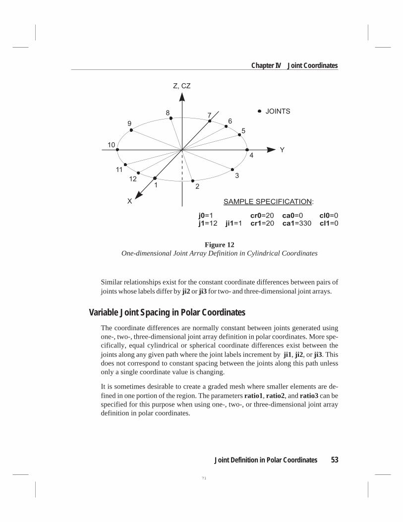
Similar relationships exist for the constant coordinate differences between pairs ofjoints whose labels differ byji2 or ji3 for two- and three-dimensional joint arrays.
Variable Joint Spacing in Polar Coordinates
The coordinate differences are normally constant between joints generated usingone-, two-, three-dimensional joint array definition in polar coordinates. More spe-cifically, equal cylindrical or spherical coordinate differences exist between thejoints along any given path where the joint labels increment byji1 , ji2 , or ji3 . Thisdoes not correspond to constant spacing between the joints along this path unlessonly a single coordinate value is changing.
It is sometimes desirable to create a graded mesh where smaller elements are de-fined in one portion of the region. The parametersratio1, ratio2, andratio3 can bespecified for this purpose when using one-, two-, or three-dimensional joint arraydefinition in polar coordinates.
Joint Definition in Polar Coordinates 53
Chapter IV Joint Coordinates
Figure 12One-dimensional Joint Array Definition in Cylindrical Coordinates
71

In cylindrical coordinates, parameterratio1 gives the ratio of the coordinate differ-ences,∆cr1n , ∆ca1n , and∆cz1n , between jointsj1–ji1 and j1, and the coordinate
differences,∆cr11 , ∆ca11 , and∆cz11 , between jointsj0 andj0+ji1 :
ratio1 = = =∆
∆
∆
∆
∆
∆
cr
cr
ca
ca
cz
cz
1n
11
1n
11
1n
11
In spherical coordinates the coordinate differences are∆sb1n , ∆sa1n , and∆sr1n and∆sb11 , ∆sa11 , and∆sr11 , respectively, and:
ratio1 = = =∆
∆
∆
∆
∆
∆
sb
sb
sa
sa
sr
sr
1n
11
1n
11
1n
11
Similar definitions apply forratio2 andratio3 for joints whose labels increment byji2 andji3 , respectively, in two- and three-dimensional joint arrays.
The coordinate differences in each case change by arithmetic progression so thatthedifferencebetween successive coordinate differences is constant.
See Topic “Variable Joint Spacing” (page 47) in this chapter for more information.
Joint Definition in Alternate Coordinate SystemsJoint coordinates are normally given in the global coordinate system. However, it issometimes convenient to define different parts of a structure in separate coordinatesystems. Each coordinate system has its own origin and orientation of the axes. Forexample, you might use a separate coordinate system for each wing of a building oreach bent of a bridge.
The parametercsysis used to specify which coordinate system is being used to de-fine joint coordinates:
• If csys=0, the global coordinate system is used; this is the default
• Otherwise,csysis the label of an Alternate Coordinate System
A different value ofcsysmay be used for each joint or set of joints. The coordinatesof a joint may be specified in rectangular, cylindrical, or spherical coordinates withrespect to coordinate systemcsys.
The choice of the coordinate system affects only the definition of individual jointsand joint arrays in one, two, or three dimensions. Linear generation, frontal genera-
54 Joint Definition in Alternate Coordinate Systems
SAP2000 Analysis Reference
72
tion, and edge generation are always performed in rectangular coordinates in theglobal coordinate system.
The location of each joint is converted to rectangular coordinates in the global coor-dinate system for printing in the .EKO output file.
It is important to understand that the use of an Alternate Coordinate System to lo-cate a joint has no effect upon the local coordinate system defined for that joint.
For more information:
• See Chapter “Coordinate Systems” (page 21).
• See Topic “Joint Definition” (page 32) in this chapter.
• See Subtopic “One-dimensional Joint Definition” (page 33) in this chapter.
• See Subtopic “Two-dimensional Joint Definition” (page 37) in this chapter.
• See Subtopic “Three-dimensional Joint Definition” (page 44) in this chapter.
• See Topic “Joint Definition in Polar Coordinates” (page 50) in this chapter.
Joint Definition in Alternate Coordinate Systems 55
Chapter IV Joint Coordinates
73

56 Joint Definition in Alternate Coordinate Systems
SAP2000 Analysis Reference
74

C h a p t e r V
Joint Patterns
Joint Patterns can be used to describe complicated spatial distributions of loadsand properties over the structure. Patterns are optional and are not required for sim-ple problems.
This chapter describes the definition of the joint Patterns. Their use is described inChapter “Joints and Degrees of Freedom” (page 75) and Chapter “Load Cases”(page 279).
Advanced Topics
• Overview
• Pattern Definition
• Gradient or Hydrostatic Specification
• One-dimensional Pattern-value Generation
• Two-dimensional Pattern-value Generation
• Three-dimensional Pattern-value Generation
• Variable Pattern-value Increments
57
75

OverviewA joint Pattern consists of a set of scalar numeric values, one value for each joint ofthe structure. A Pattern can be used to describe how certain loads and propertiesvary over the structure:
• Joint spring and mass properties
• Joint force and displacement loads
• Pressure-type loads
• Temperature-type loads
Patterns are most effective for describing complicated spatial distributions of nu-meric values. Their use is optional and is not required for simple problems.
Joint Patterns do not affect the location of the joints, or have any other effect uponthe structure except as utilized in the specification of loads and properties.
Pattern values are assigned to previously-defined joints. The specification of Pat-tern values is very similar to the definition of the joint coordinates, except that onlya single value,v, is assigned to a joint in a Pattern, whereas three coordinate values,(x, y, z), are assigned during joint definition. You may define as many Patterns asyou need, each having a single value at every joint.
The generation options available for specifying joint Pattern values correspond ex-actly to the generation options for joint coordinates. If the given Pattern values for ageneration specification are proportional to thex, y, or z coordinates of the joints,then all generated values will also be proportional tox, y, orz, respectively. This isguaranteed by the properties of isoparametric interpolation (Cook, Malkus, andPlesha, 1989).
Pattern values may also be specified that vary linearly in a given gradient directionfrom zero at a given datum point. An option is available to permit only positive oronly negative values to be defined. This is useful for defining hydrostatic pressuredistributions.
Since Pattern values are scalar quantities, they are independent of any coordinatesystem.
For more information:
• See Chapter “Joints and Degrees of Freedom” (page 75).
• See Chapter “Load Cases” (page 279).
58 Overview
SAP2000 Analysis Reference
76

Pattern DefinitionFor each Pattern to be defined, you must assign a label that will be referenced when-ever you later use the Pattern to describe the variation of a load or property.
Each Pattern starts with a numeric value of zero at every joint. You then define thenumeric values at the joints using a combination of addition, resetting, and mappingspecifications as needed:
• Eachaddition specificationadds numeric values to one or more joints. The as-signed values arealgebraically addedto the values that are already present atthe joints.
• Eachresetting specificationresets the numeric values to zero at one or morejoints.
• Eachmapping specificationinterpolates or extrapolates numeric values fromcertain joints in an array to the remaining joints in the array. Mapping isnot ad-ditive, but overwrites previous numeric values at the joints.
These specifications are applied separately to each Pattern being defined.
Addition and resetting specifications may be applied to individual joints or to ar-rays of joints. Mapping specifications apply only to joint arrays. The application ofthese specifications to arrays of one, two, and three dimensions is described in theremainder of this chapter.
Gradient or Hydrostatic SpecificationYou may define Pattern values for a given array of joints that vary linearly along aspecified gradient direction from zero value at a specified datum point. You havethe option of allowing only negative values, only positive values, or both to be gen-erated this way. For example, only positive values would be desired when defininga Pattern for hydrostatic pressure.
Any Pattern values defined by a gradient specification are algebraically additive tothe values already present at the joints of the given array.
The following parameters are needed for a gradient specification:
• A fixed coordinate system,csys(the default is zero, indicating the global coor-dinate system)
• The components of the gradient,vx, vy, andvz, in coordinate systemcsys
Pattern Definition 59
Chapter V Joint Patterns
77

• The coordinates of the zero datum point,x, y, andz, in coordinate systemcsys
• The parametersetzerowhich can take on values:
– NEG, indicating to set negative values to zero
– POS, indicating to set positive values to zero
– NO, indicating to set no values to zero (this is the default)
The componentvx indicates, for example, how much the Pattern value changes perunit of distance parallel to the X axis in coordinate systemcsys.
The Pattern value,vj, defined for a jointj that has coordinates (xj, yj, zj) is given by:
(Eqn. 1)vj = vx (xj – x) + vy (yj – y) + vz (zj – z)
if vj < 0 andsetzero= NEG, thenvj = 0
if vj > 0 andsetzero= POS, thenvj = 0
In most cases, the gradient will be parallel to one of the coordinate axes, and onlyone term in the above equation is needed.
For example, consider a hydrostatic pressure distribution caused by water im-pounded behind a dam as shown in Figure 13 (page 61). The Z direction is up in theglobal coordinate system. The pressure gradient is simply given by the fluid weightdensity acting in the downward direction. Therefore,vx = 0,vy = 0 , andvz = –62.4lb/ft3 or –9810 N/m3. The zero-pressure datum can be any point on the free surfaceof the water. Thusz should be set to the elevation of the free surface in feet or me-ters, as appropriate. For hydrostatic pressure, the parametersetzeroshould bespecified as NEG so that any joints above the free surface will be assigned a zerovalue for pressure.
One-dimensional Pattern-value GenerationPattern-value generation as described in this topic is used only in the input datatext file. You may skip this topic if you are preparing your model using the SAP2000graphical user interface.
Pattern values can be generated for a one-dimensional array of joints, i.e., a set ofjoints whose labels increment uniformly along a line or curve. The generation op-tions include addition, resetting, and linear mapping.
60 One-dimensional Pattern-value Generation
SAP2000 Analysis Reference
78

Each generation option requires the specification of a joint array for which the Pat-tern values are to be generated, as described below. No other information is re-quired for a resetting specification: the Pattern values for all joints in the array areset to zero. The additional information that is required for addition and linear-mapping specifications is described in the subtopics below.
See Subtopic “One-dimensional Regular Arrays” (page 11) in Chapter “Labels, Ar-rays, and Generation” for more information.
Joint Array Specification
Every one-dimensional generation specification requires the following informationto describe the array of joints to which Pattern values are being assigned:
• The label,j0, of the joint at the start of the line or curve
• The label,j1, of the joint at the end of the line or curve
• The label increment (constant difference),ji1 , between any pair of successivejoints along the line or curve
The number of spaces,n1, between the joints along the line or curve is then givenby:
One-dimensional Pattern-value Generation 61
Chapter V Joint Patterns
Figure 13Example of a Hydrostatic Pressure Pattern
79

n1
= −j1 j0
ji1
The labels and label increment must be chosen such thatn1 is a whole, positivenumber. The total number of joints in the array, including the ends, isn1+1.
One-dimensional Addition
A set of uniformly incrementing Pattern values can be added to the joints along aline or curve by specifying:
• The information in Subtopic “Joint Array Specification” above
• The Pattern value,v0, to be added to jointj0 at the start of the line or curve
• The Pattern value,v1, to be added to jointj1 at the end of the line or curve
The Pattern values added to the intermediate joints are determined by linear inter-polation from these values such that the constant difference,∆v
1, between the val-
ues added to any pair of successive joints is given by:
∆vn
1
1
= −v1 v0
The computed values arealgebraically addedto the values that are already presentat the joints.
One-dimensional Gradient Addition
A set of Pattern values determined from a constant gradient can be added to thejoints along a line or curve by specifying:
• The information in Subtopic “Joint Array Specification” above
• The information in Topic “Gradient or Hydrostatic Specification”
The Pattern values added to the joints are determined by Equation 1 in Topic “Gra-dient or Hydrostatic Specification” (page 59) in this chapter.
The computed values arealgebraically addedto the values that are already presentat the joints.
62 One-dimensional Pattern-value Generation
SAP2000 Analysis Reference
80

One-dimensional Linear Mapping
One-dimensional linear mapping interpolates (maps) Pattern values from existingvalues at the ends of a line or curve. Before using this option, the Pattern values atthe following joints must have already been defined (or allowed to default to zero):
1. Joint j0 at the start of the line or curve
2. Joint j1 at the end of the line or curve
It is then only necessary to provide the information in Subtopic “Joint Array Speci-fication” above.
The Pattern values assigned to the intermediate joints are determined by linear in-terpolation such that the constant value difference,∆v
1, between any pair of succes-
sive joints is given by:
∆vn
1
1
= −v1 v0
The assigned values arenot additive, but instead they replace (overwrite) the valuespresent at the joints.
Two-dimensional Pattern-value GenerationPattern-value generation as described in this topic is used only in the input datatext file. You may skip this topic if you are preparing your model using the SAP2000graphical user interface.
Pattern values can be generated for a two-dimensional array of joints, i.e., a set ofjoints whose labels increment in a uniform fashion in two separate directions. Thiswill typically correspond to a four-sided region on a flat or curved surface. The gen-eration options include addition, resetting, and several types of mapping.
Each generation option requires the specification of a joint array for which the Pat-tern values are to be generated. This is described in Subtopic “Joint Array Specifi-cation” below. No other information is required for a resetting specification: thePattern values for all joints in the array are set to zero. The additional informationthat is required for addition and mapping specifications is described in the remain-ing subtopics below.
See Subtopic “Two-dimensional Regular Arrays” (page 12) in Chapter “Labels,Arrays, and Generation” for more information.
Two-dimensional Pattern-value Generation 63
Chapter V Joint Patterns
81
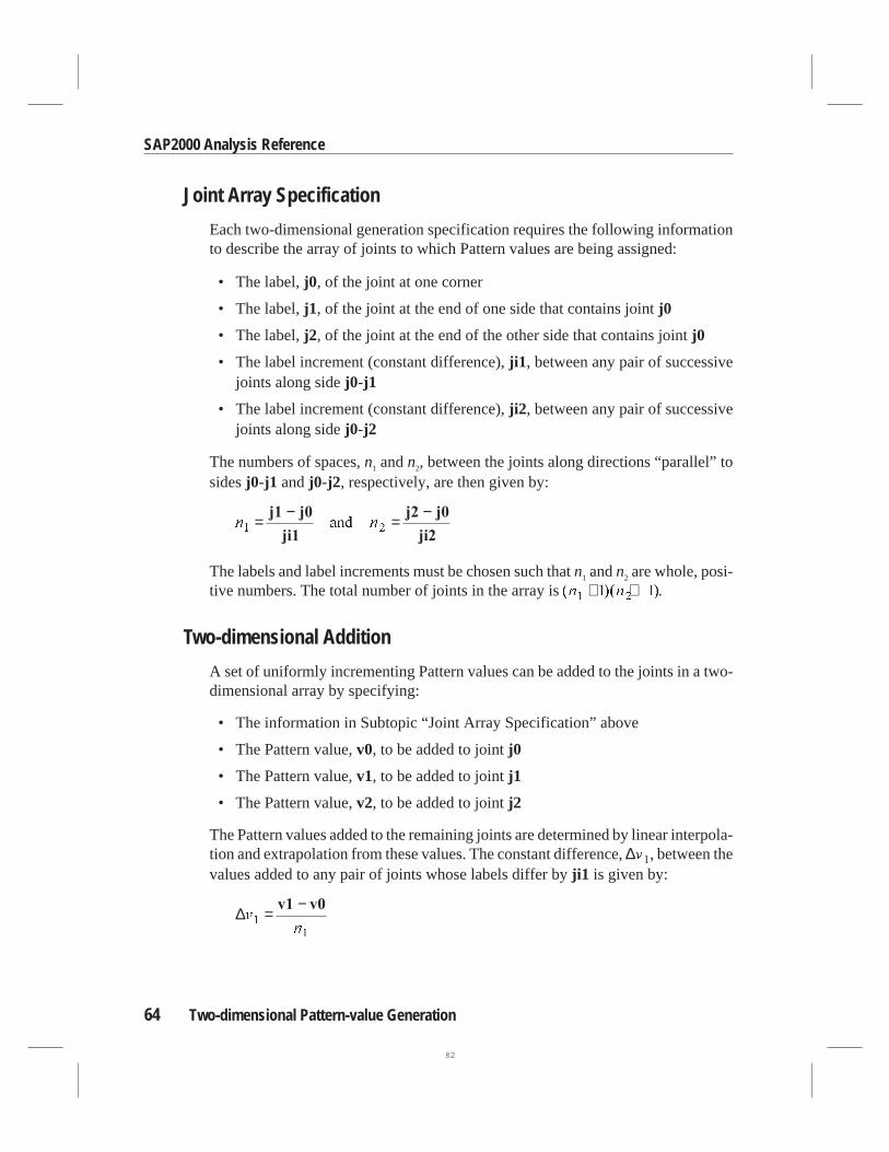
Joint Array Specification
Each two-dimensional generation specification requires the following informationto describe the array of joints to which Pattern values are being assigned:
• The label,j0, of the joint at one corner
• The label,j1, of the joint at the end of one side that contains jointj0
• The label,j2, of the joint at the end of the other side that contains jointj0
• The label increment (constant difference),ji1 , between any pair of successivejoints along sidej0-j1
• The label increment (constant difference),ji2 , between any pair of successivejoints along sidej0-j2
The numbers of spaces,n1 andn2, between the joints along directions “parallel” tosidesj0-j1 andj0-j2, respectively, are then given by:
n n1 2
= − = −j1 j0
ji1
j2 j0
ji2and
The labels and label increments must be chosen such thatn1 andn2 are whole, posi-tive numbers. The total number of joints in the array is( )( )n n
1 21 1+ + .
Two-dimensional Addition
A set of uniformly incrementing Pattern values can be added to the joints in a two-dimensional array by specifying:
• The information in Subtopic “Joint Array Specification” above
• The Pattern value,v0, to be added to jointj0
• The Pattern value,v1, to be added to jointj1
• The Pattern value,v2, to be added to jointj2
The Pattern values added to the remaining joints are determined by linear interpola-tion and extrapolation from these values. The constant difference,∆v
1, between the
values added to any pair of joints whose labels differ byji1 is given by:
∆vn
1
1
= −v1 v0
64 Two-dimensional Pattern-value Generation
SAP2000 Analysis Reference
82

Similarly, the constant difference,∆v2, between the values added to any pair of
joints whose labels differ byji2 is given by:
∆vn
2
2
= −v2 v0
The computed values arealgebraically addedto the values that are already presentat the joints.
Two-dimensional Gradient Addition
A set of Pattern values determined from a constant gradient can be added to thejoints in a two-dimensional array by specifying:
• The information in Subtopic “Joint Array Specification” above
• The information in Topic “Gradient or Hydrostatic Specification”
The Pattern values added to the joints are determined by Equation 1 in Topic “Gra-dient or Hydrostatic Specification” (page 59) in this chapter.
The computed values arealgebraically addedto the values that are already presentat the joints.
Two-dimensional Linear Mapping
Two-dimensional linear mapping interpolates (maps) a set of Pattern values over afour-sided region from existing values at the four corners. Before using this option,the Pattern values at the corner joints must have already been defined (or allowed todefault to zero):
1. Joint j0
2. Joint j1
3. Joint j2
4. Joint j1+j2–j0 at the corner opposite jointj0
It is then only necessary to provide the information in Subtopic “Joint Array Speci-fication” above.
The Pattern values assigned to the remaining joints are determined by standard bi-linear interpolation. Any subset of the joints having labels that increment uniformlyby ji1 or ji2 will have a constant difference between the generated Pattern values.
Two-dimensional Pattern-value Generation 65
Chapter V Joint Patterns
83

The assigned values arenot additive, but instead they replace (overwrite) the valuespresent at the joints.
Two-dimensional Frontal Mapping
Two-dimensional frontal mapping extrapolates (maps) a set of Pattern values overa four-sided region from existing values along two adjacent sides. Before using thisoption, the Pattern values at all joints on the two adjacent sides must have alreadybeen defined (or allowed to default to zero):
1. Jointsj0 to j1 by incrementji1 along one side
2. Jointsj0 to j2 by incrementji2 along the adjacent side
It is then only necessary to provide the information in Subtopic “Joint Array Speci-fication” above.
The Pattern values assigned to the remaining joints are determined so that:
• Any subset of the joints having labels that increment uniformly byji1 will havedifferences between the generated Pattern values that are the same as for thecorresponding joints along sidej0-j1
• Any subset of the joints having labels that increment uniformly byji2 will havedifferences between the generated Pattern values that are the same as for thecorresponding joints along sidej0-j2
The assigned values arenot additive, but instead they replace (overwrite) the valuespresent at the joints.
Two-dimensional Edge Mapping
Two-dimensional edge mapping interpolates (maps) a set of Pattern values over afour-sided region from existing values along all four sides. Before using this option,the Pattern values at all joints on the four sides must have already been defined (orallowed to default to zero):
1. Jointsj0 to j1 by incrementji1
2. Jointsj0 to j2 by incrementji2
3. Jointsj2 to j1+j2–j0 by incrementji1
4. Jointsj1 to j1+j2–j0 by incrementji2
66 Two-dimensional Pattern-value Generation
SAP2000 Analysis Reference
84

It is then only necessary to provide the information in Subtopic “Joint Array Speci-fication” above.
The Pattern values assigned to the remaining joints are determined by serendipitypolynomial interpolation (Cook, Malkus, and Plesha, 1989).
The assigned values arenot additive, but instead they replace (overwrite) the valuespresent at the joints.
Three-dimensional Pattern-value GenerationPattern-value generation as described in this topic is used only in the input datatext file. You may skip this topic if you are preparing your model using the SAP2000graphical user interface.
Pattern values can be generated for a three-dimensional array of joints, i.e., a set ofjoints whose labels increment in a uniform fashion in three separate directions. Thiswill typically correspond to a three-dimensional region enclosed by a hexahedron,i.e., having six faces. The generation options include addition, resetting, and sev-eral types of mapping.
Each generation option requires the specification of a joint array for which the Pat-tern values are to be generated. This is described in Subtopic “Joint Array Specifi-cation” below. No other information is required for a resetting specification: thePattern values for all joints in the array are set to zero. The additional informationthat is required for addition and mapping specifications is described in the remain-ing subtopics below.
Three-dimensional Pattern-value generation is a generalization of two-dimensionalPattern-value generation.
For more information:
• See Topic “Two-dimensional Pattern-value Generation” (page 63) in this chap-ter.
• See Subtopic “Three-dimensional Regular Arrays” (page 13) in Chapter “La-bels, Arrays, and Generation.”
Joint Array Specification
Each three-dimensional generation specification requires the following informa-tion to describe the array of joints to which Pattern values are being assigned:
Three-dimensional Pattern-value Generation 67
Chapter V Joint Patterns
85

• The label,j0, of the joint at one corner
• The label,j1, of the joint at the end of one side that contains jointj0
• The label,j2, of the joint at the end of another side that contains jointj0
• The label,j3, of the joint at the end of the third side that contains jointj0
• The label increment (constant difference),ji1 , between any pair of successivejoints along sidej0-j1
• The label increment (constant difference),ji2 , between any pair of successivejoints along sidej0-j2
• The label increment (constant difference),ji3 , between any pair of successivejoints along sidej0-j3
The numbers of spaces,n1, n2, andn3, between the joints along directions “parallel”to sidesj0-j1, j0-j2, andj0-j3, respectively, are then given by:
n n n1 2 3
= − = − = −j1 j0
ji1
j2 j0
ji2
j3 j0
ji3, , and
The labels and label increments must be chosen such thatn1, n2, andn3 are whole,positive numbers. The total number of joints in the array is( )( )( )n n n
1 2 31 1 1+ + + .
Three-dimensional Addition
A set of uniformly incrementing Pattern values can be added to the joints in athree-dimensional array by specifying:
• The information in Subtopic “Joint Array Specification” above
• The Pattern value,v0, to be added to jointj0
• The Pattern value,v1, to be added to jointj1
• The Pattern value,v2, to be added to jointj2
• The Pattern value,v3, to be added to jointj3
The Pattern values added to the remaining joints are determined by linear interpola-tion and extrapolation from these values. The constant difference,∆v
1, between the
values added to any pair of joints whose labels differ byji1 is given by:
∆vn
1
1
= −v1 v0
68 Three-dimensional Pattern-value Generation
SAP2000 Analysis Reference
86

Similarly, the constant difference,∆v2, between the values added to any pair of
joints whose labels differ byji2 is given by:
∆vn
2
2
= −v2 v0
Finally, the constant difference,∆v3, between the values added to any pair of joints
whose labels differ byji3 is given by:
∆vn
3
3
= −v3 v0
The computed values arealgebraically addedto the values that are already presentat the joints.
Three-dimensional Gradient Addition
A set of Pattern values determined from a constant gradient can be added to thejoints in a three-dimensional array by specifying:
• The information in Subtopic “Joint Array Specification” above
• The information in Topic “Gradient or Hydrostatic Specification”
The Pattern values added to the joints are determined by Equation 1 in Topic “Gra-dient or Hydrostatic Specification” (page 59) in this chapter.
The computed values arealgebraically addedto the values that are already presentat the joints.
Three-dimensional Linear Mapping
Three-dimensional linear mapping interpolates (maps) a set of Pattern values over ahexahedral (six-faced) region from existing values at the eight corners. Before us-ing this option, the Pattern values at the corner joints must have already been de-fined (or allowed to default to zero):
1. Joint j0
2. Joint j1
3. Joint j2
4. Joint j3
Three-dimensional Pattern-value Generation 69
Chapter V Joint Patterns
87

5. Joint j1+j2–j0 at the corner opposite jointj3
6. Joint j1+j3–j0 at the corner opposite jointj2
7. Joint j2+j3–j0 at the corner opposite jointj1
8. Joint j1+j2+j3–j0–j0 at the corner opposite jointj0
It is then only necessary to provide the information in Subtopic “Joint Array Speci-fication” above.
The Pattern values assigned to the remaining joints are determined by standard tri-linear interpolation. Any subset of the joints having labels that increment uniformlyby ji1 , ji2 , or ji3 will have a constant difference between the generated Pattern val-ues.
The assigned values arenot additive, but instead they replace (overwrite) the valuespresent at the joints.
Three-dimensional Frontal Mapping
Three-dimensional frontal mapping extrapolates (maps) a set of Pattern values overa hexahedral (six-faced) region from existing values along three adjacent edges.Before using this option, the Pattern values at all joints on the three adjacent edgesmust have already been defined (or allowed to default to zero):
1. Jointsj0 to j1 by incrementji1 along one edge
2. Jointsj0 to j2 by incrementji2 along an adjacent edge
3. Jointsj0 to j3 by incrementji3 along the other adjacent edge
It is then only necessary to provide the information in Subtopic “Joint Array Speci-fication” above.
The Pattern values assigned to the remaining joints are determined so that:
• Any subset of the joints having labels that increment uniformly byji1 will havedifferences between the generated Pattern values that are the same as for thecorresponding joints along edgej0-j1
• Any subset of the joints having labels that increment uniformly byji2 will havedifferences between the generated Pattern values that are the same as for thecorresponding joints along edgej0-j2
70 Three-dimensional Pattern-value Generation
SAP2000 Analysis Reference
88

• Any subset of the joints having labels that increment uniformly byji3 will havedifferences between the generated Pattern values that are the same as for thecorresponding joints along edgej0-j3
The assigned values arenot additive, but instead they replace (overwrite) the valuespresent at the joints.
Three-dimensional Edge Mapping
Three-dimensional edge mapping interpolates (maps) a set of Pattern values over ahexahedral (six-faced) region from existing values along all twelve edges. Beforeusing this option, the Pattern values at all joints on the twelve edges must have al-ready been defined (or allowed to default to zero):
1. Jointsj0 to j1 by incrementji1
2. Jointsj0 to j2 by incrementji2
3. Jointsj0 to j3 by incrementji3
4. Jointsj1 to j1+j2–j0 by incrementji2
5. Jointsj1 to j1+j3–j0 by incrementji3
6. Jointsj2 to j1+j2–j0 by incrementji1
7. Jointsj2 to j2+j3–j0 by incrementji3
8. Jointsj3 to j1+j3–j0 by incrementji1
9. Jointsj3 to j2+j3–j0 by incrementji2
10. Jointsj1+j2–j0 to j1+j2+j3–j0–j0 by incrementji3
11. Jointsj1+j3–j0 to j1+j2+j3–j0–j0 by incrementji2
12. Jointsj2+j3–j0 to j1+j2+j3–j0–j0 by incrementji1
It is then only necessary to provide the information in Subtopic “Joint Array Speci-fication” above.
The Pattern values assigned to the remaining joints are determined by serendipitypolynomial interpolation (Zienkiewicz and Taylor, 1989).
The assigned values arenot additive, but instead they replace (overwrite) the valuespresent at the joints.
Three-dimensional Pattern-value Generation 71
Chapter V Joint Patterns
89

Variable Pattern-value IncrementsVariable pattern-value increments as described in this topic are used only in the in-put data text file. You may skip this topic if you are preparing your model using theSAP2000 graphical user interface.
Pattern values generated by an addition specification or a linear-mapping specifica-tion normally have a constant increment (difference) between successive jointsalong any line or curve in a joint array, provided that the joint labels differ by one ofthe specified label increments.
Sometimes, however, it is desirable to have the increment in Pattern values varygradually along these lines or curves. The principal situation where this is useful iswhen you want the Pattern values to be proportional to thex, y, or zcoordinates ofthe joints and the joint spacing is not constant, as in a graded mesh.
The addition and linear-mapping specifications for Pattern values permit the use ofthe parametersratio1, ratio2, andratio3 to control the variation of generated Pat-tern values. The effect of these parameters is analogous to their effect upon jointspacing in joint array definition and joint linear mapping.
To generate Pattern values proportional to thex, y, or z coordinates of joints thatwere created using joint array definition:
• Use an addition specification for the same joint array
• Specify pattern values that are proportional to thex, y, or z coordinates of thejoints, as desired
• Specify the same values of the parametersratio1, ratio2, andratio3 as used forthe joint array definition
To generate Pattern values proportional to thex, y, or z coordinates of joints thatwere created using joint linear generation:
• Use a linear-mapping specification for the same joint array
• Make sure that the Pattern values at the corners have already been defined to beproportional to thex, y, orz coordinates of the joints, as desired
• Specify the same values of the parametersratio1, ratio2, andratio3 as usedfor the joint linear generation
The increments in Pattern values change by arithmetic progression so that thedif-ferencebetween successive increments is constant.
72 Variable Pattern-value Increments
SAP2000 Analysis Reference
90

This option is only available for addition and linear-mapping specifications. Forfrontal-mapping and edge-mapping specifications, the increments in Pattern valuesis determined from the values at the joints along the previously-defined edges.
Theratio parameters are described in more detail in the subtopics below.
For more information:
• See Topic “Variable Joint Spacing” (page 47) in Chapter “Joint Coordinates.”
• See Subtopic “One-dimensional Addition” (page 62) in this chapter.
• See Subtopic “One-dimensional Linear Mapping” (page 63) in this chapter.
• See Subtopic “Two-dimensional Addition” (page 64) in this chapter.
• See Subtopic “Two-dimensional Linear Mapping” (page 65) in this chapter.
• See Subtopic “Three-dimensional Addition” (page 68) in this chapter.
• See Subtopic “Three-dimensional Linear Mapping” (page 69) in this chapter.
One Dimension
The parameterratio1 can be used to specify how the Pattern-value increment variesalong the line of generation. It gives the ratio of the last increment,∆v1n , betweenthe values at jointsj1–ji1 andj1, and the first increment,∆v11 , between the values
at jointsj0 andj0+ji1 :
ratio1 =∆
∆
v
v
1n
11
If the value ofratio1 is greater than unity, then the increment increases along thelength. If the value ofratio1 is less than unity, then the reverse would be true. Thedefault value of unity indicates a uniform Pattern-value increment.
Two Dimensions
The two parametersratio1 andratio2 can be used to specify how the Pattern-valueincrement varies along two generation dimensions. Parameterratio1 is definedabove. Parameterratio2 is defined similarly: it gives the ratio of the last increment,∆v 2n , between the values at jointsj2–ji2 andj2, and the first increment,∆v 21 , be-
tween the values at jointsj0 andj0+ji2 :
Variable Pattern-value Increments 73
Chapter V Joint Patterns
91

ratio2 =∆
∆
v
v
2n
21
If the value ofratio1 is greater than unity, then the increment increases away fromside j0-j2 along any line or curve where the joint labels increment byji1 . If thevalue ofratio1 is less than unity, then the reverse would be true. The default valueof unity indicates a uniform Pattern-value increment.
Similarly, if the value ofratio2 is greater than unity, then the increment increasesaway from sidej0-j1 along any line or curve where the joint labels increment byji2 .If the value ofratio2 is less than unity, then the reverse would be true. The defaultvalue of unity indicates a uniform Pattern-value increment.
Three Dimensions
The three parametersratio1, ratio2 and ratio3 can be used to specify how thePattern-value increment varies along three generation dimensions. Parametersra-tio1 andratio2 are defined above. Parameterratio3 is defined similarly: it givesthe ratio of the last increment,∆v3n , between the values at jointsj3–ji3 andj3, and
the first increment,∆v31 , between the values at jointsj0 andj0+ji3 :
ratio3 =∆
∆
v
v
3n
31
If the value ofratio1 is greater than unity, then the increment increases away fromfacej0-j2-j3 along any line or curve where the joint labels increment byji1 . If thevalue ofratio1 is less than unity, then the reverse would be true. The default valueof unity indicates a uniform Pattern-value increment.
Similarly, if the value ofratio2 is greater than unity, then the increment increasesaway from facej0-j1-j3 along any line or curve where the joint labels increment byji2 . If the value ofratio2 is less than unity, then the reverse would be true. The de-fault value of unity indicates a uniform Pattern-value increment.
Finally, if the value ofratio3 is greater than unity, then the increment increasesaway from facej0-j1-j2 along any line or curve where the joint labels increment byji3 . If the value ofratio3 is less than unity, then the reverse would be true. The de-fault value of unity indicates a uniform Pattern-value increment.
74 Variable Pattern-value Increments
SAP2000 Analysis Reference
92

C h a p t e r VI
Joints and Degrees of Freedom
The joints play a fundamental role in the analysis of any structure. Joints are thepoints of connection between the elements, and they are the primary locations in thestructure at which the displacements are known or are to be determined. The dis-placement components (translations and rotations) at the joints are called thede-grees of freedom.
This chapter describes joint properties, degrees of freedom, loads, and output.Chapter “Joint Coordinates” (page 31) describes the use of joints to define the ge-ometry of the structure. Additional information about joints and degrees of freedomis given in Chapter “Constraints and Welds” (page 113).
Basic Topics for All Users
• Overview
• Modeling Considerations
• Local Coordinate System
• Degrees of Freedom
• Restraints and Reactions
• Springs
• Masses
75
93

• Force Load
• Restraint Displacement Load
• Spring Displacement Load
• Degree of Freedom Output
• Joint Mass Output
• Displacement and Acceleration Output
• Force Output
• Global Force Balance Output
Advanced Topics
• Advanced Local Coordinate System
OverviewJoints, also known asnodal pointsornodes, are a fundamental part of every struc-tural model. Joints perform a variety of functions:
• All elements are connected to the structure (and hence to each other) at thejoints
• The structure is supported at the joints using Restraints and/or Springs
• Rigid-body behavior and symmetry conditions can be specified using Con-straints that apply to the joints
• Concentrated loads may be applied at the joints
• Lumped (concentrated) masses and rotational inertia may be placed at thejoints
• All loads and masses applied to the elements are actually transferred to thejoints
• Joints are the primary locations in the structure at which the displacements areknown (the supports) or are to be determined
All of these functions are discussed in this chapter except for the Constraints, whichare described in Chapter “Constraints and Welds” (page 113).
The method used to define the structural model affects how joints are created:
76 Overview
SAP2000 Analysis Reference
94

• Using the SAP2000 graphical interface — joints are automatically created atthe ends of each Frame or Nllink element and at the corners of each Shell ele-ment; additional joints may also be defined independently of any element
• Using the input data text file — joint locations must be explicitly defined in or-der to describe the geometry of the structure; these joints are then connected byelements to build the structure
The use of joints to define the geometry of the structure is discussed in Chapter“Joint Coordinates” (page 31).
Joints act independently of each other unless connected by elements. Frame andNllink elements connect to the joints at the element ends. The two- and three-dimensional elements connect to the joints at the element corners, and possibly atother points on the element.
The joints may themselves be considered as elements with no connectivity. Eachjoint may have its own local coordinate system for defining the degrees of freedom,Restraints, joint properties, and loads; and for interpreting joint output. In mostcases, however, the global X-Y-Z coordinate system is used as the local coordinatesystem for all joints in the model.
There are six displacement degrees of freedom at every joint — three translationsand three rotations. These displacement components are aligned along the local co-ordinate system of each joint.
Joints may be loaded directly by concentrated loads or indirectly by ground dis-placements acting though Restraints or spring supports.
Displacements (translations and rotations) are produced at every joint. The externaland internal forces and moments acting on each joint are also produced.
For more information:
• See Chapter “Joint Coordinates” (page 31).
• See Chapter “Constraints and Welds” (page 113).
Modeling ConsiderationsThe location of the joints and elements is critical in determining the accuracy of thestructural model. Some of the factors that you need to consider when defining theelements, and hence the joints, for the structure are:
Modeling Considerations 77
Chapter VI Joints and Degrees of Freedom
95

• The number of elements should be sufficient to describe the geometry of thestructure. For straight lines and edges, one element is adequate. For curves andcurved surfaces, one element should be used for every arc of 15° or less.
• Element boundaries, and hence joints, should be located at points, lines, andsurfaces of discontinuity:
– Structural boundaries, e.g., corners and edges
– Changes in material properties
– Changes in thickness and other geometric properties
– Support points (Restraints and Springs)
– Points of application of concentrated loads, except that Frame elementsmay have concentrated loads applied within their spans
• In regions having large stress gradients, i.e., where the stresses are changingrapidly, a Shell element mesh should be refined using small elements andclosely-spaced joints. This may require changing the mesh after one or morepreliminary analyses.
• More that one element should be used to model the length of any span for whichdynamic behavior is important. This is required because the mass is alwayslumped at the joints, even if it is contributed by the elements.
Local Coordinate SystemEach joint has its ownjoint local coordinate systemused to define the degrees offreedom, Restraints, properties, and loads at the joint; and for interpreting joint out-put. The axes of the joint local coordinate system are denoted 1, 2, and 3. By defaultthese axes are identical to the global X, Y, and Z axes, respectively. Both systemsare right-handed coordinate systems.
The default local coordinate system is adequate for most situations. However, forcertain modeling purposes it may be useful to use different local coordinate systemsat some or all of the joints. This is described in the next topic.
For more information:
• See Topic “Upward and Horizontal Directions” (page 23) in Chapter “Coordi-nate Systems.”
• See Topic “Advanced Local Coordinate System” (page 79) in this chapter.
78 Local Coordinate System
SAP2000 Analysis Reference
96

Advanced Local Coordinate SystemBy default, the joint local 1-2-3 coordinate system is identical to the global X-Y-Zcoordinate system, as described in the previous topic. However, it may be neces-sary to use different local coordinate systems at some or all joints in the followingcases:
• Skewed Restraints (supports) are present
• Constraints are used to impose rotational symmetry
• Constraints are used to impose symmetry about a plane that is not parallel to aglobal coordinate plane
• The principal axes for the joint mass (translational or rotational) are not alignedwith the global axes
• Joint displacement and force output is desired in another coordinate system
Joint local coordinate systems need only be defined for the affected joints. Theglobal system is used for all joints for which no local coordinate system is explicitlyspecified.
A variety of methods are available to define a joint local coordinate system. Thesemay be used separately or together. Local coordinate axes may be defined to be par-allel to arbitrary coordinate directions in an arbitrary coordinate system or to vec-tors between pairs of joints. In addition, the joint local coordinate system may bespecified by a set of three joint coordinate angles. These methods are described inthe subtopics that follow.
For more information:
• See Chapter “Coordinate Systems” (page 21).
• See Topic “Local Coordinate System” (page 78) in this chapter.
Reference Vectors
To define a joint local coordinate system you must specify tworeference vectorsthat are parallel to one of the joint local coordinate planes. Theaxis reference vec-tor , Va , must be parallel to one of the local axes (i = 1, 2, or 3) in this plane and have
a positive projection upon that axis. Theplane reference vector, Vp, must have a
positive projection upon the other local axis (j = 1, 2, or 3, buti ≠ j) in this plane, butneed not be parallel to that axis. Having a positive projection means that the posi-
Advanced Local Coordinate System 79
Chapter VI Joints and Degrees of Freedom
97

tive direction of the reference vector must make an angle of less than 90° with thepositive direction of the local axis.
Together, the two reference vectors define a local axis,i, and a local plane,i-j. Fromthis, the program can determine the third local axis,k, using vector algebra.
For example, you could choose the axis reference vector parallel to local axis 1 andthe plane reference vector parallel to the local 1-2 plane (i = 1, j = 2). Alternatively,you could choose the axis reference vector parallel to local axis 3 and the plane ref-erence vector parallel to the local 3-2 plane (i = 3, j = 2). You may choose the planethat is most convenient to define using the parameterlocal, which may take on thevalues 12, 13, 21, 23, 31, or 32. The two digits correspond toi andj, respectively.The default is value is 31.
Defining the Axis Reference Vector
To define the axis reference vector for jointj , you must first specify or use the de-fault values for:
• A coordinate directionaxdir (the default is +Z)
• A fixed coordinate systemcsys(the default is zero, indicating the global coor-dinate system)
You may optionally specify:
• A pair of joints,axvecaandaxvecb (the default for each is zero, indicatingjoint j itself). If both are zero, this option is not used.
For each joint, the axis reference vector is determined as follows:
1. A vector is found from jointaxvecato joint axvecb. If this vector is of finitelength, it is used as the reference vectorVa
2. Otherwise, the coordinate directionaxdir is evaluated at jointj in fixed coordi-nate systemcsys, and is used as the reference vectorVa
Defining the Plane Reference Vector
To define the plane reference vector for jointj , you must first specify or use the de-fault values for:
• A primary coordinate directionpldirp (the default is +X)
80 Advanced Local Coordinate System
SAP2000 Analysis Reference
98

• A secondary coordinate directionpldirs (the default is +Y). Directionspldirsandpldirp should not be parallel to each other unless you are sure that they arenot parallel to local axis 1
• A fixed coordinate systemcsys(the default is zero, indicating the global coor-dinate system). This will be the same coordinate system that was used to definethe axis reference vector, as described above
You may optionally specify:
• A pair of joints,plvecaandplvecb(the default for each is zero, indicating jointj itself). If both are zero, this option is not used.
For each joint, the plane reference vector is determined as follows:
1. A vector is found from jointplveca to joint plvecb. If this vector is of finitelength and is not parallel to local axisi, it is used as the reference vectorVp
2. Otherwise, the primary coordinate directionpldirp is evaluated at jointj infixed coordinate systemcsys. If this direction is not parallel to local axisi, it isused as the reference vectorVp
3. Otherwise, the secondary coordinate directionpldirs is evaluated at jointj infixed coordinate systemcsys. If this direction is not parallel to local axisi, it isused as the reference vectorVp
4. Otherwise, the method fails and the analysis terminates. This will never happenif pldirp is not parallel topldirs
A vector is considered to be parallel to local axisi if the sine of the angle betweenthem is less than 10-3.
Determining the Local Axes from the Reference Vectors
The program uses vector cross products to determine the local axes from the refer-ence vectors. The three axes are represented by the three unit vectorsV
1, V
2and
V3, respectively. The vectors satisfy the cross-product relationship:
V V V1 2 3
= ×
The local axisVi is given by the vectorVa after it has been normalized to unitlength.
The remaining two axes,Vj andVk , are defined as follows:
Advanced Local Coordinate System 81
Chapter VI Joints and Degrees of Freedom
99

• If i andj permute in a positive sense, i.e.,local = 12, 23, or 31, then:
V V Vk i p= × and
V V Vj k i= ×
• If i andj permute in a negative sense, i.e.,local = 21, 32, or 13, then:
V V Vk p i= × and
V V Vj i k= ×
An example showing the determination of the joint local coordinate system usingreference vectors is given in Figure 14 (page 82).
Joint Coordinate Angles
The joint local coordinate axes determined from the reference vectors may be fur-ther modified by the use of threejoint coordinate angles, denoteda, b, andc. Inthe case where the default reference vectors are used, the joint coordinate angles de-fine the orientation of the joint local coordinate system with respect to the globalaxes.
82 Advanced Local Coordinate System
SAP2000 Analysis Reference
Figure 14Example of the Determination of the Joint Local Coordinate System
Using Reference Vectors forlocal=31
100
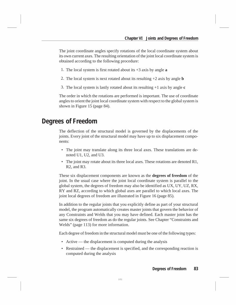
The joint coordinate angles specify rotations of the local coordinate system aboutits own current axes. The resulting orientation of the joint local coordinate system isobtained according to the following procedure:
1. The local system is first rotated about its +3 axis by anglea
2. The local system is next rotated about its resulting +2 axis by angleb
3. The local system is lastly rotated about its resulting +1 axis by anglec
The order in which the rotations are performed is important. The use of coordinateangles to orient the joint local coordinate system with respect to the global system isshown in Figure 15 (page 84).
Degrees of FreedomThe deflection of the structural model is governed by the displacements of thejoints. Every joint of the structural model may have up to six displacement compo-nents:
• The joint may translate along its three local axes. These translations are de-noted U1, U2, and U3.
• The joint may rotate about its three local axes. These rotations are denoted R1,R2, and R3.
These six displacement components are known as thedegrees of freedomof thejoint. In the usual case where the joint local coordinate system is parallel to theglobal system, the degrees of freedom may also be identified as UX, UY, UZ, RX,RY and RZ, according to which global axes are parallel to which local axes. Thejoint local degrees of freedom are illustrated in Figure 16 (page 85).
In addition to the regular joints that you explicitly define as part of your structuralmodel, the program automatically creates master joints that govern the behavior ofany Constraints and Welds that you may have defined. Each master joint has thesame six degrees of freedom as do the regular joints. See Chapter “Constraints andWelds” (page 113) for more information.
Each degree of freedom in the structural model must be one of the following types:
• Active — the displacement is computed during the analysis
• Restrained — the displacement is specified, and the corresponding reaction iscomputed during the analysis
Degrees of Freedom 83
Chapter VI Joints and Degrees of Freedom
101

84 Degrees of Freedom
SAP2000 Analysis Reference
Figure 15Use of Joint Coordinate Angles to Orient the Joint Local Coordinate System
102

• Constrained — the displacement is determined from the displacements at otherdegrees of freedom
• Null — the displacement does not affect the structure and is ignored by theanalysis
• Unavailable — the displacement has been explicitly excluded from the analysis
These different types of degrees of freedom are described in the following subtop-ics.
Available and Unavailable Degrees of Freedom
You may explicitly specify the global degrees of freedom that are available to everyjoint in the structural model. By default, all six degrees of freedom are available toevery joint. This default should generally be used for all three-dimensional struc-tures.
For certain planar structures, however, you may wish to restrict theavailable de-grees of freedom. For example, in the X-Y plane: a planar truss needs only UX andUY; a planar frame needs only UX, UY, and RZ; and a planar grid or flat plateneeds only UZ, RX, and RY.
The degrees of freedom that are not specified as being available are calledunavail-able degrees of freedom. Any stiffness, loads, mass, Restraints, or Constraints thatare applied to the unavailable degrees of freedom are ignored by the analysis.
Degrees of Freedom 85
Chapter VI Joints and Degrees of Freedom
Figure 16The Six Displacement Degrees of Freedom in the Joint Local Coordinate System
103

The available degrees of freedom are always referred to the global coordinate sys-tem, and they are the same for every joint in the model. If any joint local coordinatesystems are used, they must not couple available degrees of freedom with the un-available degrees of freedom at any joint. For example, if the available degrees offreedom are UX, UY, and RZ, then all joint local coordinate systems must have onelocal axis parallel to the global Z axis.
Restrained Degrees of Freedom
If the displacement of a joint along any one of its available degrees of freedom isknown, such as at a support point, that degree of freedom isrestrained. The knownvalue of the displacement may be zero or non-zero, and may be different in differ-ent Load Cases. The force along the restrained degree of freedom that is required toimpose the specified restraint displacement is called the reaction, and is determinedby the analysis.
Unavailable degrees of freedom are essentially restrained. However, they are ex-cluded from the analysis and no reactions are computed, even if they are non-zero.
See Topic “Restraints and Reactions” (page 88) in this chapter for more informa-tion.
Constrained Degrees of Freedom
Any joint that is part of a Constraint or Weld may have one or more of its availabledegrees of freedomconstrained. The program automatically creates a master jointto govern the behavior of each Constraint, and a master joint to govern the behaviorof each set of joints that are connected together by a Weld. The displacement of aconstrained degree of freedom is then computed as a linear combination of the dis-placements along the degrees of freedom at the corresponding master joint.
A degree of freedommay notbe both constrained and restrained.
See Chapter “Constraints and Welds” (page 113) for more information.
Active Degrees of Freedom
All available degrees of freedom that are neither constrained nor restrained must beeither active or null. The program will automatically determine theactive degreesof freedomas follows:
86 Degrees of Freedom
SAP2000 Analysis Reference
104

• If any load or stiffness is applied alonganytranslational degree of freedom at ajoint, then all available translational degrees of freedom at that joint are madeactive unless they are constrained or restrained.
• If any load or stiffness is applied alongany rotational degree of freedom at ajoint, then all available rotational degrees of freedom at that joint are made ac-tive unless they are constrained or restrained.
• All degrees of freedom at a master joint that govern constrained degrees offreedom are made active.
A joint that is connected to any element or to a translational spring will have all ofits translational degrees of freedom activated. A joint that is connected to a Frame,Shell, or Nllink element, or to any rotational spring will have all of its rotational de-grees of freedom activated. An exception is a Frame element with only truss-typestiffness, which will not activate rotational degrees of freedom.
Every active degree of freedom has an associated equation to be solved. If there areN active degrees of freedom in the structure, there areN equations in the system,and the structural stiffness matrix is said to be of orderN. The amount of computa-tional effort required to perform the analysis increases withN.
The load acting along each active degree of freedom is known (it may be zero). Thecorresponding displacement will be determined by the analysis.
If there are active degrees of freedom in the system at which the stiffness is knownto be zero, such as the out-of-plane translation in a planar-frame, these must eitherbe restrained or made unavailable. Otherwise, the structure is unstable and the solu-tion of the static equations will fail.
For more information:
• See Topic “Springs” (page 89) in this chapter.
• See Topic “Degrees of Freedom” (page 147) in Chapter “The Frame Element.”
• See Topic “Degrees of Freedom” (page 185) in Chapter “The Shell Element.”
• See Topic “Degrees of Freedom” (page 208) in Chapter “The Plane Element.”
• See Topic “Degrees of Freedom” (page 224) in Chapter “The Asolid Element.”
• See Topic “Degrees of Freedom” (page 236) in Chapter “The Solid Element.”
• See Topic “Degrees of Freedom” (page 245) in Chapter “The Nllink Element.”
Degrees of Freedom 87
Chapter VI Joints and Degrees of Freedom
105

Null Degrees of Freedom
The available degrees of freedom that are not restrained, constrained, or active, arecalled the null degrees of freedom. Because they have no load or stiffness, their dis-placements and reactions are zero, and they have no effect on the rest of the struc-ture. The program automatically excludes them from the analysis.
Joints that have no elements connected to them typically have all six degrees offreedom null. Joints that have only solid-type elements (Plane, Asolid, and Solid)connected to them typically have the three rotational degrees of freedom null.
Restraints and ReactionsIf the displacement of a joint along any of its available degrees of freedom has aknown value, either zero (e.g., at support points) or non-zero (e.g., due to supportsettlement), aRestraint must be applied to that degree of freedom. The knownvalue of the displacement may differ from one Load Case to the next, but the degreeof freedom is restrained for all Load Cases. In other words, it is not possible to havethe displacement known in one Load Case and unknown (unrestrained) in anotherLoad Case.
Restraints should also be applied to available degrees of freedom in the system atwhich the stiffness is known to be zero, such as the out-of-plane translation and in-plane rotations of a planar-frame. Otherwise, the structure is unstable and the solu-tion of the static equations will fail.
Restraints are always applied to the joint local degrees of freedom U1, U2, U3, R1,R2, and R3. However, it is permissible to specify restraints in terms of the globaldegrees of freedom UX, UY, UZ, RX, RY, and RZ. If a local degree of freedom isfound at the joint that is parallel to the specified global degree of freedom, the re-straint is applied to that local degree of freedom. If no parallel local degree of free-dom is found,then the specified restraint is not applied.
The force or moment along the degree of freedom that is required to enforce the re-straint is called thereaction, and it is determined by the analysis. The reaction maydiffer from one Load Case to the next. The reaction includes the forces (or mo-ments) from all elements and springs connected to the restrained degree of free-dom, as well as all loads applied to the degree of freedom.
A restrained degree of freedom may not be constrained. If a restraint is applied to anunavailable degree of freedom, it is ignored and no reaction is computed.
88 Restraints and Reactions
SAP2000 Analysis Reference
106

Examples of Restraints are shown in Figure 17 (page 90).
For more information:
• See Topic “Degrees of Freedom” (page 83) in this chapter.
• See Topic “Restraint Displacement Load” (page 93) in this chapter.
SpringsAny of the six degrees of freedom at any of the joints in the structure can have trans-lational or rotational spring support conditions. These springs elastically connectthe joint to the ground. Spring supports along restrained degrees of freedom do notcontribute to the stiffness of the structure.
Springs may be specified that couple the degrees of freedom at a joint. The springforces that act on a joint are related to the displacements of that joint by a 6x6 sym-metric matrix of spring stiffness coefficients. These forces tend to oppose the dis-placements.
Spring stiffness coefficients may be specified in the global coordinate system, anAlternate Coordinate System, or the joint local coordinate system.
In a joint local coordinate system, the spring forces and momentsF1, F2, F3, M1, M2
andM3 at a joint are given by:
(Eqn. 1)F
F
F
M
M
M
1
2
3
1
2
3
= −
u1 u1u2 u1u3 u1r1 u1r2 u1r3
u2 u2u3 u2r1 u2r2 u2r3
u3 u3r1 u3r2 u3r3
r1 r1r2 r1r3
sym. r2 r2r3
r3
u
u
u
r
r
r
1
2
3
1
2
3
whereu1, u2, u3, r1, r2 andr3 are the joint displacements and rotations, and the termsu1, u1u2, u2, ... are the specified spring stiffness coefficients.
In any fixed coordinate system, the spring forces and momentsFx, Fy, Fz, Mx, My andMz at a joint are given by:
Springs 89
Chapter VI Joints and Degrees of Freedom
107

90 Springs
SAP2000 Analysis Reference
Figure 17Examples of Restraints
108

F
F
F
M
M
M
x
y
z
x
y
z
= −
ux uxuy uxuz uxrx uxry uxrz
uy uyuz uyrx uyry uyrz
uz uzrx uzry uzrz
rx rxry rxrz
sym. ry ryrz
rz
u
u
u
r
r
r
x
y
z
x
y
z
whereux, uy, uz, rx, ry andrz are the joint displacements and rotations, and the termsux, uxuy, uy, ... are the specified spring stiffness coefficients.
For springs that do not couple the degrees of freedom in a particular coordinate sys-tem, only the six diagonal terms need to be specified since the off-diagonal termsare all zero. When coupling is present, all 21 coefficients in the upper triangle of thematrix must be given; the other 15 terms are then known by symmetry.
If the springs at a joint are specified in more than one coordinate system, standardcoordinate transformation techniques are used to convert the 6x6 spring stiffnessmatrices to the joint local coordinate system, and the resulting stiffness matrices arethen added together on a term-by-term basis. The final spring stiffness matrix ateach joint in the structure should have a determinant that is zero or positive. Other-wise the springs may cause the structure to be unstable.
The displacement of the grounded end of the spring may be specified to be zero ornon-zero (e.g., due to support settlement). Thisspring displacementmay varyfrom one Load Case to the next.
For more information:
• See Topic “Degrees of Freedom” (page 83) in this chapter.
• See Topic “Spring Displacement Load” (page 95) in this chapter.
MassesIn a dynamic analysis, the mass of the structure is used to compute inertial forces.Normally, the mass is obtained from the elements using the mass density of the ma-terial and the volume of the element. This automatically produces lumped (uncou-pled) masses at the joints. The element mass values are equal for each of the threetranslational degrees of freedom. No mass moments of inertia are produced for therotational degrees of freedom. This approach is adequate for most analyses.
Masses 91
Chapter VI Joints and Degrees of Freedom
109

It is often necessary to place additional concentrated masses and/or mass momentsof inertia at the joints. These can be applied to any of the six degrees of freedom atany of the joints in the structure.
For computational efficiency and solution accuracy, SAP2000 always uses lumpedmasses. This means that there is no mass coupling between degrees of freedom at ajoint or between different joints. These uncoupled masses are always referred to thelocal coordinate system of each joint. Mass values along restrained degrees of free-dom are ignored.
Inertial forces acting on the joints are related to the accelerations at the joints by a6x6 matrix of mass values. These forces tend to oppose the accelerations. In a jointlocal coordinate system, the inertia forces and momentsF1, F2, F3, M1, M2 andM3 ata joint are given by:
F
F
F
M
M
M
1
2
3
1
2
3
= −
u1 0 0 0 0 0
u2 0 0 0 0
u3 0 0 0
r1 0 0
sym. r2 0
r3
&&
&&
&&
&&
&&
u
u
u
r
r
1
2
3
1
2
3&&r
where&&u1, &&u
2, &&u
3, &&r
1, &&r
2and&&r
3are the translational and rotational accelerations at
the joint, and the termsu1, u2, u3, r1, r2, andr3 are the specified mass values.
Uncoupled joint masses may instead be specified in the global coordinate system,in which case they are transformed to the joint local coordinate system. Couplingterms will be generated during this transformation in the following situation:
• The joint local coordinate system directions are not parallel to global coordi-nate directions, and
• The three translational masses or the three rotational mass moments of inertiaare not equal at a joint.
These coupling terms will be discarded by the program, resulting in some loss ofaccuracy. For this reason, it is recommended that you choose joint local coordinatesystems that are aligned with the principal directions of translational or rotationalmass at a joint, and then specify mass values in these joint local coordinates.
Mass values must be given in consistent mass units (W/g) and mass moments of in-ertia must be inWL2/g units. HereW is weight,L is length, andg is the acceleration
92 Masses
SAP2000 Analysis Reference
110

due to gravity. The net mass values at each joint in the structure should be zero orpositive.
See Figure 18 (page 94) for mass moment of inertia formulations for various planarconfigurations.
For more information:
• See Topic “Degrees of Freedom” (page 83) in this chapter.
• See Chapter “Static and Dynamic Analysis” (page 291).
Force LoadThe Force Load is used to apply concentrated forces and moments at the joints. Val-ues may be specified in a fixed coordinate system (global or alternate coordinates)or the joint local coordinate system. All forces and moments at a joint are trans-formed to the joint local coordinate system and added together. The specified val-ues are shown in Figure 19 (page 95).
Forces and moments applied along restrained degrees of freedom add to the corre-sponding reaction, but do not otherwise affect the structure.
For more information:
• See Topic “Degrees of Freedom” (page 83) in this chapter.
• See Chapter “Load Cases” (page 279).
Restraint Displacement LoadThe Restraint Displacement Load is used to apply specified displacements (transla-tions and rotations) at thegrounded endof joint restraints. Restraint displacementsmay be specified in a fixed coordinate system (global or alternate coordinates) orthe joint local coordinate system. The specified values are shown in Figure 19 (page95). All displacements at a joint are transformed to the joint local coordinate systemand added together.
Restraints may be considered as rigid connections between the joint degrees offreedom and the ground, and are always defined in the joint local coordinate sys-tem. If a particular joint degree of freedom is restrained, the displacement of thejoint is equal to the restraint displacement along that local degree of freedom. Com-
Force Load 93
Chapter VI Joints and Degrees of Freedom
111

94 Restraint Displacement Load
SAP2000 Analysis Reference
Figure 18Formulae for Mass Moments of Inertia
112

ponents of restraint displacement that are not along restrained degrees of freedomdo not load the structure. An example of this is illustrated in Figure 20 (page 96).
For more information:
• See Topic “Restraints and Reactions” (page 88) in this chapter.
• See Chapter “Load Cases” (page 279).
Spring Displacement LoadThe Spring Displacement Load is used to apply specified displacements (transla-tions and rotations) at thegrounded endof joint spring supports. Spring displace-ments may be specified in a fixed coordinate system (global or alternate coordi-nates) or the joint local coordinate system. The specified values are shown in Figure19 (page 95).
All displacements at a joint are transformed to the joint local coordinate system andadded together. The resulting displacements are multiplied by the spring stiffness
Spring Displacement Load 95
Chapter VI Joints and Degrees of Freedom
Figure 19Specified Values for Force Load, Restraint Displacement Load,
and Spring Displacement Load
113
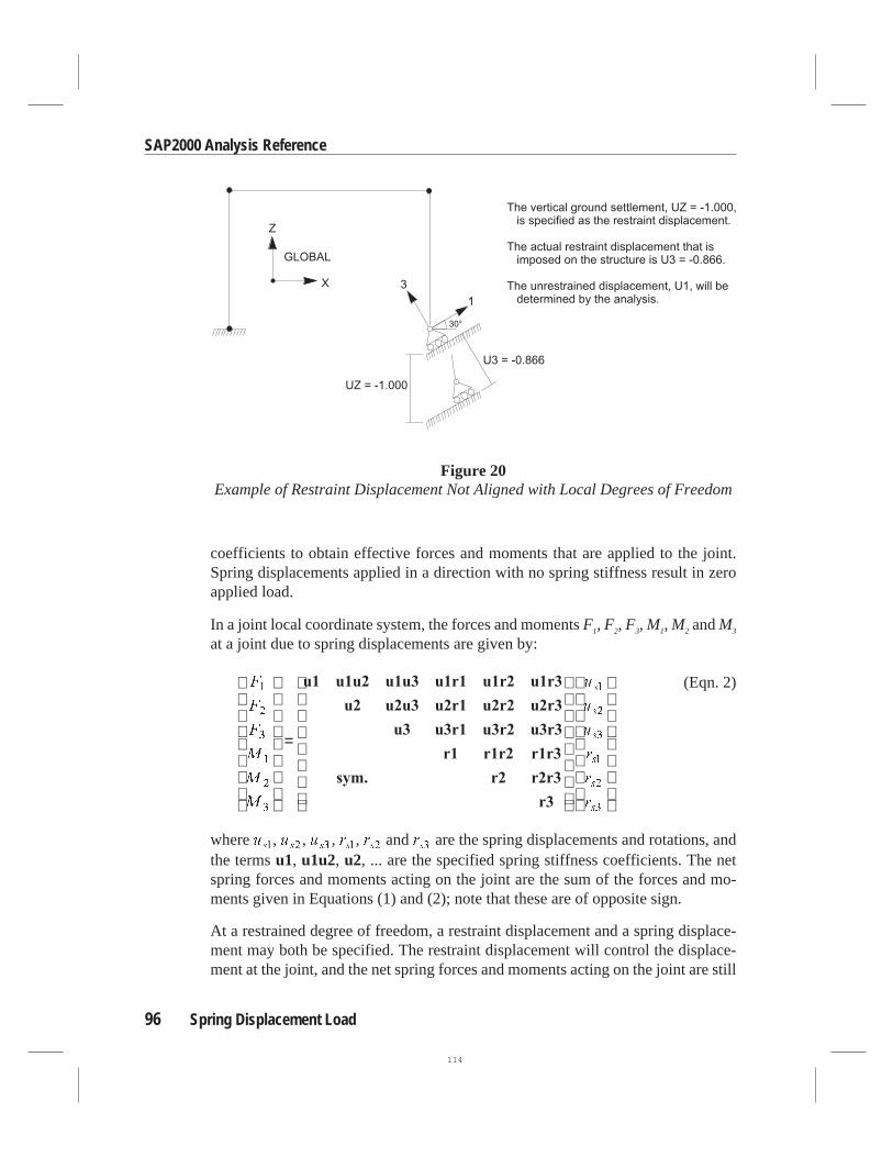
coefficients to obtain effective forces and moments that are applied to the joint.Spring displacements applied in a direction with no spring stiffness result in zeroapplied load.
In a joint local coordinate system, the forces and momentsF1, F2, F3, M1, M2 andM3
at a joint due to spring displacements are given by:
(Eqn. 2)F
F
F
M
M
M
1
2
3
1
2
3
=
u1 u1u2 u1u3 u1r1 u1r2 u1r3
u2 u2u3 u2r1 u2r2 u2r3
u3 u3r1 u3r2 u3r3
r1 r1r2 r1r3
sym. r2 r2r3
r3
u
u
u
r
r
r
s
s
s
s
s
s
1
2
3
1
2
3
whereus1, us2 , us3 , rs1, rs2 andrs3 are the spring displacements and rotations, andthe termsu1, u1u2, u2, ... are the specified spring stiffness coefficients. The netspring forces and moments acting on the joint are the sum of the forces and mo-ments given in Equations (1) and (2); note that these are of opposite sign.
At a restrained degree of freedom, a restraint displacement and a spring displace-ment may both be specified. The restraint displacement will control the displace-ment at the joint, and the net spring forces and moments acting on the joint are still
96 Spring Displacement Load
SAP2000 Analysis Reference
Figure 20Example of Restraint Displacement Not Aligned with Local Degrees of Freedom
114

given by the sum of the forces and moments of Equations (1) and (2). An exampleof this is illustrated in Figure 21 (page 97).
For more information:
• See Topic “Springs” (page 89) in this chapter.
• See Chapter “Load Cases” (page 279).
Degree of Freedom OutputA table of the types of degrees of freedom present at every joint in the model isprinted in the output file under the heading:
DISPLACEMENT DEGREES OF FREEDOM
The degrees of freedom are listed for all of the regular joints, as well as for the mas-ter joints created automatically by the program. For Constraints, the master jointsare identified by the labels of their corresponding Constraints. For Welds, the mas-ter joint for each set of joints that are welded together is identified by the label ofone of the welded joints. Joints are printed in alpha-numeric order of the labels.
Degree of Freedom Output 97
Chapter VI Joints and Degrees of Freedom
Figure 21Interaction Between Restraint Displacements and Spring Displacements
115

The type of each of the six degrees of freedom at a joint is identified by the follow-ing symbols:
(A) Active degree of freedom(-) Restrained degree of freedom(+) Constrained degree of freedom( ) Null or unavailable degree of freedom
The degrees of freedom are always referred to the local axes of the joint. They areidentified in the output as U1, U2, U3, R1, R2, and R3 for all joints. However, if allregular joints use the global coordinate system as the local system (the usual situa-tion), then the degrees of freedom for the regular joints are identified as UX, UY,UZ, RX, RY, and RZ.
The types of degrees of freedom are a property of the structure and are independentof the Analysis Cases.
Typical degree-of-freedom output is shown in Figure 22 (page 99).
For more information:
• See Topic “Degrees of Freedom” (page 83) in this chapter.
• See Chapter “The Output Files” (page 395).
Joint Mass OutputA table of the assembled masses at every joint in the model is printed in the outputfile under the heading:
ASSEMBLED JOINT MASSES
The mass at a given joint includes the mass assigned directly to that joint as well asa portion of the mass from each element connected to that joint. Mass at restraineddegrees of freedom is set to zero. All mass assigned to the elements is apportionedto the connected joints, so that this table represents the totalunrestrainedmass ofthe structure.
Joints are printed in alpha-numeric order of the labels. Joints that have no unre-strained mass are not printed.
The masses are always referred to the local axes of the joint. They are identified inthe output as U1, U2, U3, R1, R2, and R3. However, if all joints use the global coor-
98 Joint Mass Output
SAP2000 Analysis Reference
116

dinate system as the local system (the usual situation), then the masses are identi-fied as UX, UY, UZ, RX, RY, and RZ.
Joint Mass Output 99
Chapter VI Joints and Degrees of Freedom
D I S P L A C E M E N T D E G R E E S O F F R E E D O M
(A) = Active DOF, equilibrium equation(-) = Restrained DOF, reaction computed(+) = Constrained DOF( ) = Null DOF
JOINTS UX UY UZ RX RY RZ1 TO 2 - + +3 + + +4 + + + + - -5 - + + + - +6 TO 7 - + +8 + + +9 + + + + - -
10 A + + + A +11 TO 12 - + +13 + + +14 + + + + - -15 - + + + - +16 TO 17 - + +18 + + +19 + + + + - -20 - + + + - +21 TO 22 - + +23 + + +24 + + + + - -25 A + + + A +26 TO 27 - + +28 + + +29 + + + + - -30 - + + + - +31 TO 34 + + + + + +35 TO 36 - - - - - -
CONSTRAINTS U1 U2 U3 R1 R2 R3PLATE A A ASYM01 TO SYM02 A ASYM03 A A ASYM04 A A A ASYM05 ASYM06 TO SYM07 A ASYM08 A A ASYM09 A A A ASYM10 ASYM11 TO SYM12 A ASYM13 A A ASYM14 A A A ASYM15 ASYM31 TO SYM33 A A A A A A
Figure 22Degree of Freedom Table in File EXAMPLE.OUT
117

The total unrestrained masses of the structure,Mx, My, andMz, acting in the globalX, Y, and Z directions, are printed in the output file under the heading:
TOTAL UNRESTRAINED MASS AND LOCATION
These three masses may differ even if the three translational masses assigned toeach joint are equal, since the restraints for the three translational degrees of free-dom at a joint need not be the same.
The locations of the centers of mass forMx, My, andMz are given with respect to theglobal origin. These can be used together with the mass values to determine the mo-ments caused by the Acceleration Loads.
For more information:
• See Topic “Masses” (page 91) in this chapter.
• See Chapter “Static and Dynamic Analysis” (page 291).
• See Chapter “The Output Files” (page 395).
Displacement and Acceleration OutputJoint displacement output is available for the following types of Analysis Cases:Loads, Modes, Specs, Histories, Moving Loads, and Combos. History results arethe maximum and minimum values attained during the analysis, and are only avail-able if specifically requested in the definition of the individual History cases.
Joint translations and rotations are printed in the output file under the heading:
JOINT DISPLACEMENTS
The displacements at all joints are printed together for each Analysis Case. Jointsare presented in alpha-numeric order. The displacements are given only for theavailable degrees of freedom. No results are printed for any joint that has only nullor unavailable degrees of freedom.
The displacements are always referred to the local axes of the joint. They are identi-fied in the output as U1, U2, U3, R1, R2, and R3. However, if all joints use theglobal coordinate system as the local system (the usual situation), then the displace-ments are identified as UX, UY, UZ, RX, RY, and RZ.
Typical joint displacement output is shown in Figure 23 (page 101).
100 Displacement and Acceleration Output
SAP2000 Analysis Reference
118

Displacement and Acceleration Output 101
Chapter VI Joints and Degrees of Freedom
J O I N T D I S P L A C E M E N T S
TRANSLATIONS AND ROTATIONS, IN GLOBAL COORDINATES
LOAD 1 ------------------
JOINT UX UY UZ RX RY RZ1 .000000 -0.008161 0.076681 .000000 .000000 .0000002 .000000 -0.007954 0.060396 .000000 .000000 .0000003 0.000108 -0.007493 0.044780 .000000 .000000 .0000004 0.000103 -0.006662 0.030495 -0.001115 .000000 .0000005 .000000 -0.005493 0.018238 -0.000915 .000000 4.68E-356 .000000 1.45E-17 0.076676 .000000 .000000 .0000007 .000000 2.50E-17 0.060375 .000000 .000000 .0000008 3.09E-18 2.77E-17 0.044741 .000000 .000000 .0000009 2.26E-18 1.92E-17 0.030437 -0.001115 .000000 .000000
10 -6.57E-19 1.62E-17 0.018137 -0.000915 -2.79E-05 4.68E-3511 .000000 0.008161 0.076681 .000000 .000000 .00000012 .000000 0.007954 0.060396 .000000 .000000 .00000013 -0.000108 0.007493 0.044780 .000000 .000000 .00000014 -0.000103 0.006662 0.030495 -0.001115 .000000 .000000
COMB BOTH ------------------ MAX
JOINT UX UY UZ RX RY RZ1 .000000 -0.007855 0.079786 .000000 .000000 .0000002 .000000 -0.007650 0.062892 .000000 .000000 .0000003 0.000111 -0.007198 0.046676 .000000 .000000 .0000004 0.000106 -0.006389 0.031820 -0.001070 .000000 .0000005 .000000 -0.005258 0.019050 -0.000876 .000000 2.65E-116 .000000 3.16E-05 0.079780 .000000 .000000 .0000007 .000000 3.08E-05 0.062871 .000000 .000000 .0000008 5.36E-07 2.87E-05 0.046637 .000000 .000000 .0000009 4.92E-07 2.46E-05 0.031760 -0.001070 .000000 .000000
10 7.20E-07 1.97E-05 0.018946 -0.000876 -2.69E-05 2.65E-1111 .000000 0.008467 0.079786 .000000 .000000 .00000012 .000000 0.008257 0.062892 .000000 .000000 .00000013 -0.000105 0.007789 0.046676 .000000 .000000 .00000014 -0.000100 0.006936 0.031820 -0.001070 .000000 .000000
COMB BOTH ------------------ MIN
JOINT UX UY UZ RX RY RZ1 .000000 -0.008467 0.073577 .000000 .000000 .0000002 .000000 -0.008257 0.057900 .000000 .000000 .0000003 0.000105 -0.007789 0.042884 .000000 .000000 .0000004 0.000100 -0.006936 0.029171 -0.001161 .000000 .0000005 .000000 -0.005728 0.017425 -0.000955 .000000 -2.65E-116 .000000 -3.16E-05 0.073571 .000000 .000000 .0000007 .000000 -3.08E-05 0.057879 .000000 .000000 .0000008 -5.36E-07 -2.87E-05 0.042846 .000000 .000000 .0000009 -4.92E-07 -2.46E-05 0.029114 -0.001161 .000000 .000000
10 -7.20E-07 -1.97E-05 0.017329 -0.000955 -2.89E-05 -2.65E-1111 .000000 0.007855 0.073577 .000000 .000000 .00000012 .000000 0.007650 0.057900 .000000 .000000 .00000013 -0.000111 0.007198 0.042884 .000000 .000000 .00000014 -0.000106 0.006389 0.029171 -0.001161 .000000 .000000
...Output Truncated for Brevity...
Figure 23Joint Displacements in the Output File
119

By default, no displacements are printed. You may specify which Analysis Casesare to be printed. The joint displacements can always be displayed using theSAP2000 graphical interface even if no results have been selected for printing.
For Response-spectrum casesonly, acceleration output will also be provided at anyjoint for which joint displacements are requested. Joint translational and rotationalaccelerations are printed in the output file under the heading:
JOINT ACCELERATIONS
The format of the joint acceleration output is identical to that for joint displace-ments.
It is important to note that the Response Spectrum results are always positive, andthat the correspondence between different values has been lost.
For more information:
• See Topic “Degrees of Freedom” (page 83) in this chapter.
• See Chapter “Load Cases” (page 279).
• See Chapter “Static and Dynamic Analysis” (page 291).
• See Chapter “The Output Files” (page 395).
Force OutputJoint force output is available for the following types of Analysis Cases: Loads,Modes, Specs, Histories (restricted), Moving Loads (restricted), and Combos. His-tory results are the maximum and minimum values attained during the analysis, andare only available if specifically requested in the definition of the History case.
The forces and moments that act on the joints come from a variety of sources:
• Applied loads
• Inertial loads
• Stiffness forces
• Spring forces
• Nllink forces
• Restraint Forces (Reactions)
• Constraint forces
• P-delta forces
102 Force Output
SAP2000 Analysis Reference
120
For Histories, Moving Loads, and Combos that contain Histories or Moving Loads,only spring forces and reactions are available.
The forces and moments from each different source are computed and printed sepa-rately in the output file, as discussed in the subtopics below.
The forces and moments are always referred to the local axes of the joint. They areidentified in the output as F1, F2, F3, M1, M2, and M3. However, if all joints usethe global coordinate system as the local system (the usual situation), then theforces and moments are identified as FX, FY, FZ, MX, MY, and MZ.
The values printed are always the forces and moments thatact onthe joints. Thus apositive value of joint force or moment tends to cause a positive value of joint trans-lation or rotation along the corresponding degree of freedom.
The forces and moments for all joints are printed together for each Analysis Case.Joints are presented in alpha-numeric order. Values are given only for the availabledegrees of freedom. No results are printed for any joint that has only null or unavail-able degrees of freedom.
By default, no force output is produced. You may specify which Analysis Cases areto be printed. Certain joint forces and moments can be displayed using theSAP2000 graphical interface even if no results have been selected for printing.
It is important to note that the Response Spectrum results are always positive, andthat the correspondence between different values has been lost.
For more information:
• See Topic “Degrees of Freedom” (page 83) in this chapter.
• See Chapter “Load Cases” (page 279).
• See Chapter “Static and Dynamic Analysis” (page 291).
• See Chapter “P-Delta Analysis” (page 337).
• See Chapter “The Output Files” (page 395).
Applied Loads
The applied loads include all specified loads that act directly on the joints and thosethat act on elements connected to the joints. These specified loads include Force,Self-Weight, Gravity, Temperature, Concentrated Span, Distributed Span,Prestress, Uniform, Surface Pressure, Pore Pressure, and Rotate Loads. The effects
Force Output 103
Chapter VI Joints and Degrees of Freedom
121

of the Restraint Displacement and Spring Displacement Loads are not includedhere.
Joint forces and moments due to applied loads are printed in the output file underthe heading:
APPLIED LOADS
Results are given only for joints that have at least one non-zero force or momentvalue. The applied loads are always zero for Mode and Spec Analysis Cases.
Typical applied-load output is shown in Figure 24 (page 105).
Inertial Loads
The inertial loads are the effective, or D’Alembert, forces and moments which re-sist acceleration. For a Vibration Mode of frequencyω, the acceleration for transla-tional degree of freedomi at a joint is given by−ω2
u i , whereui is the translation.
Hence the inertial forceFi for that degree of freedom is given by:
F m ui ui i= − ω2
wheremuiis the mass for degree of freedomi at the joint. Similarly, the inertial mo-
mentMi for rotational degree of freedomi at a joint is given by:
M m ri ri i= − ω2
whereri is the rotation andmriis the mass moment of inertia for degree of freedomi
at the joint.
The displacement at a restrained degree of freedom is always zero in a VibrationMode, hence the inertial loads are always zero for these degrees of freedom.
The inertial loads for Spec and Combo Analysis Cases are just the appropriate com-binations of the inertial loads for the contributing Modes. The inertial loads for theLoad Cases are always zero.
Joint forces and moments due to inertial loads are printed in the output file underthe heading:
INERTIAL LOADS
104 Force Output
SAP2000 Analysis Reference
122

Force Output 105
Chapter VI Joints and Degrees of Freedom
A P P L I E D L O A D S
FORCES AND MOMENTS ACTING ON JOINTS, IN GLOBAL COORDINATES
LOAD 1 ------------------
JOINT FX FY FZ MX MY MZ1 .000000 .000000 167.000000 .000000 .000000 .0000006 .000000 .000000 666.000000 .000000 .000000 .000000
11 .000000 .000000 167.000000 .000000 .000000 .00000016 .000000 .000000 167.000000 .000000 .000000 .00000021 .000000 .000000 666.000000 .000000 .000000 .00000026 .000000 .000000 167.000000 .000000 .000000 .000000
COMB STATIC ------------------ MAX
JOINT FX FY FZ MX MY MZ1 .000000 .000000 167.000000 .000000 .000000 .0000006 .000000 .000000 666.000000 .000000 .000000 .000000
11 .000000 .000000 167.000000 .000000 .000000 .00000016 .000000 .000000 167.000000 .000000 .000000 .00000021 .000000 .000000 666.000000 .000000 .000000 .00000026 .000000 .000000 167.000000 .000000 .000000 .000000
COMB STATIC ------------------ MIN
JOINT FX FY FZ MX MY MZ1 .000000 .000000 167.000000 .000000 .000000 .0000006 .000000 .000000 666.000000 .000000 .000000 .000000
11 .000000 .000000 167.000000 .000000 .000000 .00000016 .000000 .000000 167.000000 .000000 .000000 .00000021 .000000 .000000 666.000000 .000000 .000000 .00000026 .000000 .000000 167.000000 .000000 .000000 .000000
COMB BOTH ------------------ MAX
JOINT FX FY FZ MX MY MZ1 .000000 .000000 167.000000 .000000 .000000 .0000006 .000000 .000000 666.000000 .000000 .000000 .000000
11 .000000 .000000 167.000000 .000000 .000000 .00000016 .000000 .000000 167.000000 .000000 .000000 .00000021 .000000 .000000 666.000000 .000000 .000000 .00000026 .000000 .000000 167.000000 .000000 .000000 .000000
COMB BOTH ------------------ MIN
JOINT FX FY FZ MX MY MZ1 .000000 .000000 167.000000 .000000 .000000 .0000006 .000000 .000000 666.000000 .000000 .000000 .000000
11 .000000 .000000 167.000000 .000000 .000000 .00000016 .000000 .000000 167.000000 .000000 .000000 .00000021 .000000 .000000 666.000000 .000000 .000000 .00000026 .000000 .000000 167.000000 .000000 .000000 .000000
Figure 24Applied Loads in the Output File
123
Results are given only for joints that have non-zero, unrestrained mass or mass mo-ments of inertia.
Stiffness Forces
The stiffness forces are the elastic forces contributed by any Frame, Shell, Plane,Asolid, and Solid elements that are connected to a joint. These forces are obtainedas the product of the element stiffness matrices and the displacements at the con-nected joints. The stiffness forces are not printed in the output file, but are used tocompute the constraint forces and reactions.
Spring Forces
The spring forces are the product of the spring stiffness coefficients and the jointdisplacements as given by Equation (1). If spring displacements are present, theseproduce additional forces as given by Equation (2).
Spring forces are printed in the output file under the heading:
SPRING FORCES
Results are given only for joints that have non-zero spring stiffness coefficients.
Nllink Forces
The Nllink forces are the elastic forces contributed by any Nllink elements that areconnected to a joint. These forces are obtained as the product of the Nllink elementstiffness matrices and the displacements at the connected joints. The Nllink stiff-ness matrices are based upon the effective-stiffness parameters. For two-joint ele-ments, the forces and moments should be self-equilibrating. For single-joint ele-ments, the forces and moments are supporting the structure.
Nllink forces are printed in the output file under the heading:
NLLINK FORCES
Results are given only for joints that are connected to Nllink elements.
Restraint Forces (Reactions)
The restraint forces are the forces and moments that are required to enforce the re-straints. These reactions are computed as the sum of the applied loads, stiffnessforces, spring forces, and Nllink forces acting on the restrained degrees of freedom.
106 Force Output
SAP2000 Analysis Reference
124

Restraint forces are printed in the output file under the heading:
RESTRAINT FORCES (REACTIONS)
Results are given only for joints that possess restrained degrees of freedom.
Typical reaction output is shown in Figure 25 (page 108).
Constraint Forces
The constraint forces are the forces and moments that are required to enforce theconstraints. These are computed as the sum of the applied loads, inertial loads, stiff-ness forces, spring forces, and Nllink forces acting on the constrained degrees offreedom. These forces and moments should be self-equilibrating over the entirestructure if the constraints are properly defined. See the next Subtopic, “GlobalForce Balance Output,” for more information.
Constraint forces are printed in the output file under the heading:
CONSTRAINT FORCES
Results are given only for joints that possess constrained degrees of freedom.
P-Delta Moments
The P-delta moments are present only when a P-Delta analysis has been performed.For each Frame element, the P-Delta moments are computed as the vector crossproduct of the acting P-Delta force in the element and the difference between thedisplacements at the two ends of the element. These individual P-Delta momentsare not assigned to specific joints or printed in the output file, but are summed andprinted as part of the global force balance.
Global Force Balance OutputFor each Analysis Case, the sum of all joint forces and moments acting on the struc-ture should be in equilibrium. The program computes and prints a global force bal-ance for the following types of Analysis Cases: Loads, Modes, Specs, and Combos;no global force balance is computed for Histories, Moving Loads, or Combos thatcontain Histories or Moving Loads. You should always review the global force bal-ance as a check on the validity of the structural model and the analysis.
Global Force Balance Output 107
Chapter VI Joints and Degrees of Freedom
125

108 Global Force Balance Output
SAP2000 Analysis Reference
R E S T R A I N T F O R C E S ( R E A C T I O N S )
FORCES AND MOMENTS ACTING ON JOINTS, IN GLOBAL COORDINATES
LOAD 1 ------------------
JOINT FX FY FZ MX MY MZ35 7.35E-13 -9.73E-11 -1000.000 84000.000 2026.122 7.47E-1236 -7.35E-13 -9.73E-11 -1000.000 84000.000 -2026.122 -7.47E-12
SPEC SPEC ------------------
JOINT FX FY FZ MX MY MZ35 0.972230 126.377896 68.323489 3978.697 89.135262 9.78850936 0.972230 126.377896 68.323489 3978.697 89.135262 9.788509
COMB STATIC ------------------ MAX
JOINT FX FY FZ MX MY MZ35 7.35E-13 -9.73E-11 -1000.000 84000.000 2026.122 7.47E-1236 -7.35E-13 -9.73E-11 -1000.000 84000.000 -2026.122 -7.47E-12
COMB STATIC ------------------ MIN
JOINT FX FY FZ MX MY MZ35 7.35E-13 -9.73E-11 -1000.000 84000.000 2026.122 7.47E-1236 -7.35E-13 -9.73E-11 -1000.000 84000.000 -2026.122 -7.47E-12
COMB DYNAMIC ------------------ MAX
JOINT FX FY FZ MX MY MZ35 0.972230 126.377896 68.323489 3978.697 89.135262 9.78850936 0.972230 126.377896 68.323489 3978.697 89.135262 9.788509
COMB DYNAMIC ------------------ MIN
JOINT FX FY FZ MX MY MZ35 -0.972230 -126.377896 -68.323489 -3978.697 -89.135262 -9.78850936 -0.972230 -126.377896 -68.323489 -3978.697 -89.135262 -9.788509
COMB BOTH ------------------ MAX
JOINT FX FY FZ MX MY MZ35 0.972230 126.377896 -931.676511 87978.697 2115.257 9.78850936 0.972230 126.377896 -931.676511 87978.697 -1936.987 9.788509
COMB BOTH ------------------ MIN
JOINT FX FY FZ MX MY MZ35 -0.972230 -126.377896 -1068.323 80021.303 1936.987 -9.78850936 -0.972230 -126.377896 -1068.323 80021.303 -2115.257 -9.788509
...Output has been Edited for Brevity
Figure 25Restraint Forces (Reactions) in the Output File
126

For each Analysis Case, the program computes the resultants at the global origin forall joint forces and moments acting on the structure. Separate resultants are com-puted for each type of joint force:
• Applied loads
• Inertial loads
• Spring forces
• Nllink forces
• Restraint Forces (Reactions)
• Constraint forces
• P-Delta forces
Each force resultant is computed as the sum of the forces acting on all joints in thestructure. Each moment resultant is computed as the sum of the moments acting onall joints in the structure, plus the moments about the origin of the forces acting onall joints in the structure. This results in three force and three moment components,all referred to the global coordinate system.
The resultants are also computed for the total of all these different forces and mo-ments acting on the structure. These total resultants should be zero if the structure isin exact equilibrium. Due to the approximate nature of computer arithmetic, the to-tals may not be exactly zero. However, their values relative to the magnitude of thecontributing forces gives a measure of the accuracy and stability of the solution.
The resultant forces and moments are always printed in the output file for all Analy-sis Cases under the heading:
GLOBAL FORCE BALANCE
Typical output is shown in Figure 26 (page 110).
In addition, relative equilibrium errors are printed in the log file under the heading:
GLOBAL FORCE BALANCE RELATIVE ERRORS
Here the total force and moment components are expressed as a percentage of themaximum possible equilibrium error. The maximum possible error is computed asfollows:
• For each component (FX, FY, FZ, MX, MY, and MZ), the absolute values ofthe resultants for applied loads, inertial loads, spring forces, Nllink forces, reac-tions, constraint forces, and P-Delta forces are summed.
• The maximum of the absolute sums for FX, FY, and FZ is determined.
Global Force Balance Output 109
Chapter VI Joints and Degrees of Freedom
127

110 Global Force Balance Output
SAP2000 Analysis Reference
G L O B A L F O R C E B A L A N C E
TOTAL FORCE AND MOMENT AT THE ORIGIN, IN GLOBAL COORDINATES
LOAD 1 ------------------
FX FY FZ MX MY MZAPPLIED .000000 .000000 2000.000 .000000 -12000.000 .000000INERTIA .000000 .000000 .000000 .000000 .000000 .000000REACTNS .000000 -1.95E-10 -2000.000 1.13E-08 12000.000 -1.17E-09CONSTRS 3.04E-11 -2.46E-11 -9.85E-10 1.86E-08 7.33E-09 -1.21E-09
TOTAL 3.04E-11 -2.19E-10 2.32E-10 3.00E-08 3.22E-11 -2.38E-09
MODE 1 ------------------
FX FY FZ MX MY MZAPPLIED .000000 .000000 .000000 .000000 .000000 .000000INERTIA -4.36E-07 -1.18E-06 -49672.588 -1.1135E+06 298035.531 1.25E-05REACTNS .000000 0.001497 49672.588 1.1135E+06 -298035.530 0.008985CONSTRS 0.000439 -0.001496 7.42E-05 0.014819 0.002190 -0.030060
TOTAL 0.000439 -3.92E-09 4.53E-09 -4.38E-07 0.002633 -0.021063
SPEC SPEC ------------------
FX FY FZ MX MY MZAPPLIED .000000 .000000 .000000 .000000 .000000 .000000INERTIA 0.000784 252.768070 136.646868 4505.715 819.881682 1516.622REACTNS .000000 252.755793 136.646979 4505.613 819.881873 1516.535CONSTRS 0.006039 0.016173 0.004416 0.444113 0.030539 0.373549
TOTAL 0.005267 1.03E-11 1.17E-11 1.14E-09 0.031604 0.252835
COMB BOTH ------------------ MAX
FX FY FZ MX MY MZAPPLIED .000000 .000000 2000.000 .000000 -12000.000 .000000INERTIA 0.000784 252.768070 136.646868 4505.715 819.881682 1516.622REACTNS .000000 252.755793 -1863.353 4505.613 12819.882 1516.535CONSTRS 0.006039 0.016173 0.004416 0.444113 0.030539 0.373549
TOTAL 0.005267 -2.09E-10 2.43E-10 3.11E-08 0.031604 0.252835
COMB BOTH ------------------ MIN
FX FY FZ MX MY MZAPPLIED .000000 .000000 2000.000 .000000 -12000.000 .000000INERTIA -0.000784 -252.768070 -136.646868 -4505.715 -819.881682 -1516.622REACTNS .000000 -252.755793 -2136.647 -4505.613 11180.118 -1516.535CONSTRS -0.006039 -0.016173 -0.004416 -0.444113 -0.030539 -0.373549
TOTAL -0.005267 -2.29E-10 2.20E-10 2.88E-08 -0.031604 -0.252835
...Output has been Edited for Brevity
Figure 26Global Force Balance in the Output File
128

• The maximum of the absolute sums for MX, MY, and MZ is determined.
• The maximum possible error for the force components is the maximum of theabsolute force sums, or the maximum of the absolute moment sums divided bythe average moment arm for the structure, whichever is larger.
• The maximum possible error for the moment components is the maximum ofthe absolute moment sums, or the maximum of the absolute force sums multi-plied by the average moment arm for the structure, whichever is larger.
This definition, while complicated, assures that only numerically meaningful equi-librium errors are indicated as such.
Typical output is shown in Figure 27 (page 111).
It is strongly recommended that you always review the global force balance in theoutput file and the relative equilibrium errors in the log file. These results can alertyou to potential problems with the structural model or the analysis. In particular,you should look for the following:
• The accuracy of the computer calculations is on the order of 10-15, or 10-13per-cent. If the relative force or moment error for the Load Cases is significantly
Global Force Balance Output 111
Chapter VI Joints and Degrees of Freedom
G L O B A L F O R C E B A L A N C E R E L A T I V E E R R O R S
PERCENT FORCE AND MOMENT ERROR AT THE ORIGIN, IN GLOBAL COORDINATES
LOAD FX FY FZ MX MY MZ1 7.60E-13 5.48E-12 5.79E-12 2.20E-11 2.36E-14 1.75E-12
MODE FX FY FZ MX MY MZ1 4.42E-07 3.94E-12 4.56E-12 1.30E-11 7.79E-08 6.23E-072 7.22E-05 2.08E-13 3.59E-14 1.42E-12 1.28E-05 0.0001023 0.000232 3.36E-13 1.62E-14 1.23E-13 0.000139 0.0011134 0.007859 3.36E-14 9.51E-15 9.00E-14 0.001394 0.011150
SPEC FX FY FZ MX MY MZSPEC 0.001042 2.03E-12 2.32E-12 1.22E-11 0.000340 0.002719
COMB MAX/MIN FX FY FZ MX MY MZSTATIC 7.60E-13 5.48E-12 5.79E-12 2.20E-11 2.36E-14 1.75E-12STATIC 7.60E-13 5.48E-12 5.79E-12 2.20E-11 2.36E-14 1.75E-12
DYNAMIC 0.001042 2.03E-12 2.32E-12 1.22E-11 0.000340 0.002719DYNAMIC 0.001042 2.03E-12 2.32E-12 1.22E-11 0.000340 0.002719
BOTH 0.000132 5.22E-12 6.09E-12 2.29E-11 2.32E-05 0.000186BOTH 0.000123 5.37E-12 5.15E-12 1.98E-11 2.17E-05 0.000174
Figure 27Global Force Balance Relative Errors in the Log File
129

larger than this, it may indicate that the structure is unstable or that the stiffnessmatrix is ill-conditioned.
• You can expect somewhat larger equilibrium errors for Vibration Modes thanfor Load Cases. For Eigen Modes, the errors generally reflect the convergencetolerance and can be reduced by using a smaller tolerance. For Ritz Modes, theerrors indicate the fact that the Ritz modes are not the true Eigen Modes of thestructure. These errors can generally be reduced by requesting more modes.Some Modes with large errors may be orthogonal to the Ritz starting vectorsand have no effect upon response-spectrum and time-history analyses.
• The constraint forces should be self-equilibrating, i.e., the resultant constraintforces and moments should be essentially zero. If the values are significantlydifferent from zero (compared to the other resultants), the constraints may bepoorly defined. An example of this is a Diaphragm constraint whose joints arenot all in the same plane: in-plane forces in the Diaphragm can cause momentsthat are not captured by the structural model. Such errors in the constraints af-fect the validity of the model even though the overall equilibrium of the struc-ture may be satisfied.
See Topic “Force Output” (page 102) in this chapter for more information.
112 Global Force Balance Output
SAP2000 Analysis Reference
130

C h a p t e r VII
Constraints and Welds
Constraintsare used to enforce certain types of rigid-body behavior, to connect to-gether different parts of the model, and to impose certain types of symmetry condi-tions.Weldsare used to generate a set of constraints that connect together differentparts of the model.
Basic Topics for All Users
• Overview
• Body Constraint
• Plane Definition
• Diaphragm Constraint
• Plate Constraint
• Axis Definition
• Rod Constraint
• Beam Constraint
• Equal Constraint
• Welds
113
131

Advanced Topics
• Local Constraint
• Automatic Master Joints
• Constraint Output
OverviewA constraint consists of a set of two or moreconstrained joints. The displacementsof each pair of joints in the constraint are related by constraint equations. The typesof behavior that can be enforced by constraints are:
• Rigid-body behavior, in which the constrained joints translate and rotate to-gether as if connected by rigid links. The types of rigid behavior that can bemodeled are:
– Rigid Body: fully rigid for all displacements
– Rigid Diaphragm: rigid for membrane behavior in a plane
– Rigid Plate: rigid for plate bending in a plane
– Rigid Rod: rigid for extension along an axis
– Rigid Beam: rigid for beam bending on an axis
• Equal-displacement behavior, in which the translations and rotations are equalat the constrained joints
• Symmetry and anti-symmetry conditions
The use of constraints reduces the number of equations in the system to be solvedand will usually result in increased computational efficiency.
Most constraint types must be defined with respect to some fixed coordinate sys-tem. The coordinate system may be the global coordinate system or an alternate co-ordinate system, or it may be automatically determined from the locations of theconstrained joints. The Local Constraint does not use a fixed coordinate system, butreferences each joint using its own joint local coordinate system.
Welds are used to connect together different parts of the model that were definedseparately. Each Weld consists of a set of joints thatmaybe joined. The programsearches for joints in each Weld that share the same location in space and constrainsthem to act as a single joint.
114 Overview
SAP2000 Analysis Reference
132

Body ConstraintA Body Constraint causes all of its constrained joints to move together as a three-dimensional rigid body. Effectively, all constrained joints are connected to eachother by rigid links and cannot displace relative to each other.
This Constraint can be used to:
• Model rigid connections, such as where several beams and/or columns frametogether
• Connect together different parts of the structural model that were defined usingseparate meshes
• Connect Frame elements that are acting as eccentric stiffeners to Shell elements
Welds can be used to automatically generate Body Constraints for the purpose ofconnectingcoincident joints.
See Topic “Welds” (page 131) in this chapter for more information.
Joint Connectivity
Each Body Constraint connects a set of two or more joints together. The joints mayhave any arbitrary location in space.
Local Coordinate System
Each Body Constraint has its own local coordinate system, the axes of which aredenoted 1, 2, and 3. These correspond to the X, Y, and Z axes of the global coordi-nate system, respectively. The actual orientation of the local axes is not importantsince the constraint equations are independent of the coordinate system.
Constraint Equations
The constraint equations relate the displacements at any two constrained joints(subscriptsi andj) in a Body Constraint. These equations are expressed in terms ofthe translations (u1, u2, andu3), the rotations (r1, r2, andr3), and the coordinates (x1,x2, andx3), all taken in the Constraint local coordinate system:
u1j = u1i + r2i ∆x3 – r3i ∆x2
u2j = u2i + r3i ∆x1 − r1i ∆x3
Body Constraint 115
Chapter VII Constraints and Welds
133

u3j = u3i + r1i ∆x2 − r2i ∆x1
r1i = r1j
r2i = r2j
r3i = r3j
where∆x1 = x1j − x1i, ∆x2 = x2j − x2i, and ∆x3 = x3j − x3i.
Plane DefinitionThe constraint equations for each Diaphragm or Plate Constraint are written withrespect to a particular plane. The location of the plane is not important, only its ori-entation.
By default, the plane is determined automatically by the program from the spatialdistribution of the constrained joints as follows:
• The centroid of the constrained joints is determined
• The second moments of the locations of all of the constrained joints about thecentroid are determined
• The principal values and directions of these second moments are found
• The direction of the smallest principal second moment is taken as the normal tothe constraint plane; if all constrained joints lie in a unique plane, this smallestprincipal moment will be zero
• If no unique direction can be found, a horizontal (X-Y) plane is assumed in co-ordinate systemcsys; this situation can occur if the joints are coincident or col-linear, or if the spatial distribution is more nearly three-dimensional than pla-nar.
You may override automatic plane selection by specifying the following:
• csys: A fixed coordinate system (the default is zero, indicating the global coor-dinate system)
• axis: The axis (X, Y, or Z) normal to the plane of the constraint, taken in coordi-nate systemcsys.
This may be useful, for example, to specify a horizontal plane for a floor with asmall step in it.
116 Plane Definition
SAP2000 Analysis Reference
134

Diaphragm ConstraintA Diaphragm Constraint causes all of its constrained joints to move together as aplanar diaphragm that is rigid against membrane deformation. Effectively, all con-strained joints are connected to each other by links that are rigid in the plane, but donot affect out-of-plane (plate) deformation.
This Constraint can be used to:
• Model concrete floors (or concrete-filled decks) in building structures, whichtypically have very high in-plane stiffness
• Model diaphragms in bridge superstructures
The use of the Diaphragm Constraint for building structures eliminates thenumerical-accuracy problems created when the large in-plane stiffness of a floordiaphragm is modeled with membrane elements. It is also very useful in the lateral(horizontal) dynamic analysis of buildings, as it results in a significant reduction inthe size of the eigenvalue problem to be solved. See Figure 28 (page 118) for an il-lustration of a floor diaphragm.
Joint Connectivity
Each Diaphragm Constraint connects a set of two or more joints together. Thejoints may have any arbitrary location in space, but for best results all joints shouldlie in the plane of the constraint. Otherwise, bending moments may be generatedthat are restrained by the Constraint, which unrealistically stiffens the structure. Ifthis happens, the constraint forces printed in the output file may not be in equilib-rium.
For more information, see:
• Topic “Force Output” (page 102) in Chapter “Joints and Degrees of Freedom.”
• Topic “Global Force Balance Output” (page 107) in Chapter “Joints and De-grees of Freedom.”
Local Coordinate System
Each Diaphragm Constraint has its own local coordinate system, the axes of whichare denoted 1, 2, and 3. Local axis 3 is always normal to the plane of the constraint.The program arbitrarily chooses the orientation of axes 1 and 2 in the plane. The ac-tual orientation of the planar axes is not important since only the normal directionaffects the constraint equations.
Diaphragm Constraint 117
Chapter VII Constraints and Welds
135

For more information, see Topic “Plane Definition” (page 116) in this chapter.
Constraint Equations
The constraint equations relate the displacements at any two constrained joints(subscriptsi and j) in a Diaphragm Constraint. These equations are expressed interms of in-plane translations (u1 andu2), the rotation (r3) about the normal, and thein-plane coordinates (x1 andx2), all taken in the Constraint local coordinate system:
u1j = u1i – r3i ∆x2
u2j = u2i + r3i ∆x1
118 Diaphragm Constraint
SAP2000 Analysis Reference
Figure 28Use of the Diaphragm Constraint to Model a Rigid Floor Slab
136

r3i = r3j
where∆x1 = x1j − x1i and ∆x2 = x2j − x2i.
Plate ConstraintA Plate Constraint causes all of its constrained joints to move together as a flat platethat is rigid against bending deformation. Effectively, all constrained joints are con-nected to each other by links that are rigid for out-of-plane bending, but do not af-fect in-plane (membrane) deformation.
This Constraint can be used to:
• Connect structural-type elements (Frame and Shell) to solid-type elements(Plane and Solid); the rotation in the structural element can be converted to apair of equal and opposite translations in the solid element by the Constraint
• Enforce the assumption that “plane sections remain plane” in detailed modelsof beam bending
Joint Connectivity
Each Plate Constraint connects a set of two or more joints together. The joints mayhave any arbitrary location in space. Unlike the Diaphragm Constraint, equilibriumis not affected by whether or not all joints lie in the plane of the Plate Constraint.
Local Coordinate System
Each Plate Constraint has its own local coordinate system, the axes of which are de-noted 1, 2, and 3. Local axis 3 is always normal to the plane of the constraint. Theprogram arbitrarily chooses the orientation of axes 1 and 2 in the plane. The actualorientation of the planar axes is not important since only the normal direction af-fects the constraint equations.
For more information, see Topic “Plane Definition” (page 116) in this chapter.
Constraint Equations
The constraint equations relate the displacements at any two constrained joints(subscriptsi andj) in a Plate Constraint. These equations are expressed in terms ofthe out-of-plane translation (u3), the bending rotations (r1 andr2), and the in-planecoordinates (x1 andx2), all taken in the Constraint local coordinate system:
Plate Constraint 119
Chapter VII Constraints and Welds
137

u3j = u3i + r1i ∆x2 − r2i ∆x1
r1i = r1j
r2i = r2j
where∆x1 = x1j − x1i and ∆x2 = x2j − x2i.
Axis DefinitionThe constraint equations for each Rod or Beam Constraint are written with respectto a particular axis. The location of the axis is not important, only its orientation.
By default, the axis is determined automatically by the program from the spatialdistribution of the constrained joints as follows:
• The centroid of the constrained joints is determined
• The second moments of the locations of all of the constrained joints about thecentroid are determined
• The principal values and directions of these second moments are found
• The direction of the largest principal second moment is taken as the axis of theconstraint; if all constrained joints lie on a unique axis, the two smallest princi-pal moments will be zero
• If no unique direction can be found, a vertical (Z) axis is assumed in coordinatesystemcsys; this situation can occur if the joints are coincident, or if the spatialdistribution is more nearly planar or three-dimensional than linear.
You may override automatic axis selection by specifying the following:
• csys: A fixed coordinate system (the default is zero, indicating the global coor-dinate system)
• axis: The axis (X, Y, or Z) of the constraint, taken in coordinate systemcsys.
This may be useful, for example, to specify a vertical axis for a column with a smalloffset in it.
Rod ConstraintA Rod Constraint causes all of its constrained joints to move together as a straightrod that is rigid against axial deformation. Effectively, all constrained joints main-
120 Axis Definition
SAP2000 Analysis Reference
138

tain a fixed distance from each other in the direction parallel to the axis of the rod,but translations normal to the axis and all rotations are unaffected.
This Constraint can be used to:
• Prevent axial deformation in Frame elements
• Model rigid truss-like links
An example of the use of the Rod Constraint is in the analysis of the two-dimensional frame shown in Figure 29 (page 121). If the axial deformations in thebeams are negligible, a single Rod Constraint could be defined containing the fivejoints. Instead of five equations, the program would use a single equation to definethe X-displacement of the whole floor. However, it should be noted that this will re-sult in the axial forces of the beams being output as zero, as the Constraint willcause the ends of the beams to translate together in the X-direction. Interpretationsof such results associated with the use of Constraints should be clearly understood.
Joint Connectivity
Each Rod Constraint connects a set of two or more joints together. The joints mayhave any arbitrary location in space, but for best results all joints should lie on theaxis of the constraint. Otherwise, bending moments may be generated that are re-
Rod Constraint 121
Chapter VII Constraints and Welds
Figure 29Use of the Rod Constraint to Model Axially Rigid Beams
139

strained by the Constraint, which unrealistically stiffens the structure. If this hap-pens, the constraint forces printed in the output file may not be in equilibrium.
For more information, see:
• Topic “Force Output” (page 102) in Chapter “Joints and Degrees of Freedom.”
• Topic “Global Force Balance Output” (page 107) in Chapter “Joints and De-grees of Freedom.”
Local Coordinate System
Each Rod Constraint has its own local coordinate system, the axes of which are de-noted 1, 2, and 3. Local axis 1 is always the axis of the constraint. The program arbi-trarily chooses the orientation of the transverse axes 2 and 3. The actual orientationof the transverse axes is not important since only the axial direction affects the con-straint equations.
For more information, see Topic “Axis Definition” (page 120) in this chapter.
Constraint Equations
The constraint equations relate the displacements at any two constrained joints(subscriptsi andj) in a Rod Constraint. These equations are expressed only in termsof the axial translation (u1):
u1j = u1i
Beam ConstraintA Beam Constraint causes all of its constrained joints to move together as a straightbeam that is rigid against bending deformation. Effectively, all constrained jointsare connected to each other by links that are rigid for off-axis bending, but do not af-fect translation along or rotation about the axis.
This Constraint can be used to:
• Connect structural-type elements (Frame and Shell) to solid-type elements(Plane and Solid); the rotation in the structural element can be converted to apair of equal and opposite translations in the solid element by the Constraint
• Prevent bending deformation in Frame elements
122 Beam Constraint
SAP2000 Analysis Reference
140
Joint Connectivity
Each Beam Constraint connects a set of two or more joints together. The joints mayhave any arbitrary location in space, but for best results all joints should lie on theaxis of the constraint. Otherwise, torsional moments may be generated that are re-strained by the Constraint, which unrealistically stiffens the structure. If this hap-pens, the constraint forces printed in the output file may not be in equilibrium.
For more information, see:
• Topic “Force Output” (page 102) in Chapter “Joints and Degrees of Freedom”
• Topic “Global Force Balance Output” (page 107) in Chapter “Joints and De-grees of Freedom”
Local Coordinate System
Each Beam Constraint has its own local coordinate system, the axes of which aredenoted 1, 2, and 3. Local axis 1 is always the axis of the constraint. The programarbitrarily chooses the orientation of the transverse axes 2 and 3. The actual orienta-tion of the transverse axes is not important since only the axial direction affects theconstraint equations.
For more information, see Topic “Axis Definition” (page 120) in this chapter.
Constraint Equations
The constraint equations relate the displacements at any two constrained joints(subscriptsi andj) in a Beam Constraint. These equations are expressed in terms ofthe transverse translations (u2 andu3), the transverse rotations (r2 andr3), and the ax-ial coordinate (x1), all taken in the Constraint local coordinate system:
u2j = u2i + r3i ∆x1
u3j = u3i − r2i ∆x1
r2i = r2j
r3i = r3j
where∆x1 = x1j − x1i.
Beam Constraint 123
Chapter VII Constraints and Welds
141

Equal ConstraintAn Equal Constraint causes all of its constrained joints to move together with thesame (or opposite) displacements for each selected degree of freedom, taken in theconstraint local coordinate system. The other degrees of freedom are unaffected.
The Equal Constraint differs from the rigid-body types of Constraints in that thereis no couplingbetween the rotations and the translations.
This Constraint can be used to:
• Model symmetry and anti-symmetry conditions with respect to a plane
• Partially connect together different parts of the structural model, such as at ex-pansion joints and hinges
For fully connecting meshes, it is better to use the Body Constraint when the con-strained joints are not in exactly the same location.
Joint Connectivity
Each Equal Constraint connects a set of two or more joints together. For a givenConstraint, ifanyof the selected degrees of freedom are negative (i.e., opposite),only two constrained joints are allowed for that Constraint. Otherwise any numberof constrained joints are permitted.
The joints may have any arbitrary location in space, but for best results all jointsshould share the same location in space if used for connecting meshes. Otherwise,moments may be generated that are restrained by the Constraint, which unrealisti-cally stiffens the structure. If this happens, the constraint forces printed in the out-put file may not be in equilibrium.
Such restrained moments may also be generated when Equal Constraints are usedfor symmetry purposes. They are necessary to enforce the desired symmetry oranti-symmetry of the displacements when the applied loads are not correspond-ingly symmetric or anti-symmetric.
For more information, see:
• Topic “Force Output” (page 102) in Chapter “Joints and Degrees of Freedom.”
• Topic “Global Force Balance Output” (page 107) in Chapter “Joints and De-grees of Freedom.”
124 Equal Constraint
SAP2000 Analysis Reference
142

Local Coordinate System
Each Equal Constraint uses a fixed coordinate system,csys, that you specify. Thedefault forcsysis zero, indicating the global coordinate system. The axes of thefixed coordinate system are denoted X, Y, and Z.
Selected Degrees of Freedom
For each Equal Constraint you may specify a list,cdofs, of up to six degrees of free-dom in coordinate systemcsysthat are to be constrained. The degrees of freedomare indicated as UX, UY, UZ, RX, RY, and RZ. A negative sign indicates a degreeof freedom that is constrained to be opposite, e.g.,−UX.
Constraint Equations
The constraint equations relate the displacements at any two constrained joints(subscriptsi andj) in an Equal Constraint. These equations are expressed in termsof the translations (ux, uy, anduz) and the rotations (rx, ry, andrz), all taken in fixed co-ordinate systemcsys. The equations used depend upon the selected degrees of free-dom and their signs. Some important cases are described next.
Symmetry About a Plane
For a structure that is symmetric about a plane, symmetric loading causes symmet-ric displacements as follows:
• Forces and displacements parallel to the plane of symmetry are equal
• Forces and displacements normal to the plane of symmetry are opposite
• Moments and rotations parallel to the plane of symmetry are opposite
• Moments and rotations normal to the plane of symmetry are equal
As an example, consider a structure that is symmetric with respect to a plane normalto the X axis and subjected to symmetric loading. A separate Equal Constraint mustbe defined for each pair of joints that is symmetrically located with respect to theplane. The degrees of freedom that would be specified for these Constraints are:−UX, UY, UZ, RX, −RY, and−RZ. The corresponding constraint equations are:
uxj = − uxi
uyj = uyi
Equal Constraint 125
Chapter VII Constraints and Welds
143

uzj = uzi
rxi = rxj
ryi = − ryj
rzi = − rzj
Any joints on the plane of symmetry should not be constrained, but instead havetheir UX, RY, and RZ degrees of freedom restrained.
Anti-symmetry About a Plane
For a structure that is symmetric about a plane, anti-symmetric loading causesanti-symmetric displacements. All degrees of freedom that are equal when sym-metric are opposite when anti-symmetric, and all degrees of freedom that are oppo-site when symmetric are equal when anti-symmetric. Thus the specification of theanti-symmetric degrees of freedom simply uses the opposite signs from the sym-metric case.
Consider the example above of a structure that is symmetric with respect to a planenormal to the X axis, but now subjected to anti-symmetric loading. A separateEqual Constraint must be defined for each pair of joints that is symmetrically lo-cated with respect to the plane. The degrees of freedom that would be specified forthese Constraints are: UX,−UY, −UZ, −RX, RY, and RZ. The signs of the con-straint equations are corresponding changed from the symmetric case.
Partial Connection
When joints are being connected, all specified degrees of freedom are positive. Forexample, consider an idealized hinge connection of eight space-truss members.Only displacements are continuous across the hinge, not rotations. Each truss mem-ber is connected to a separate joint (node) at the connection. One Equal Constraintis defined for the eight constrained joints. The degrees of freedom that would bespecified for this Constraint are: UX, UY, and UZ. The corresponding constraintequations are:
uxj = uxi
uyj = uyi
uzj = uzi
126 Equal Constraint
SAP2000 Analysis Reference
144

The eight joints should be coincident or the axes of the truss members should all in-tersect at the same point. Otherwise, moments may be generated that are unrealisti-cally restrained by the Constraint.
Local ConstraintA Local Constraint causes all of its constrained joints to move together with thesame (or opposite) displacements for each selected degree of freedom, taken in theseparate joint local coordinate systems. The other degrees of freedom are unaf-fected.
The Local Constraint differs from the rigid-body types of Constraints in that there isno couplingbetween the rotations and the translations. The Local Constraint is thesame as the Equal Constraint if all constrained joints have the same local coordinatesystem.
This Constraint can be used to:
• Model symmetry conditions with respect to a line or a point
• Model displacements constrained by mechanisms
The behavior of this Constraint is dependent upon the choice of the local coordinatesystems of the constrained joints.
Joint Connectivity
Each Local Constraint connects a set of two or more joints together. Ifanyof the se-lected degrees of freedom for a given Constraint are negative (i.e., opposite) onlytwo constrained joints are allowed for that Constraint. Otherwise any number ofconstrained joints are permitted.
The joints may have any arbitrary location in space. If the joints do not share thesame location in space, moments may be generated that are restrained by the Con-straint. If this happens, the constraint forces printed in the output file may not be inequilibrium. These moments are necessary to enforce the desired symmetry of thedisplacements when the applied loads are not symmetric, or may represent the con-straining action of a mechanism.
For more information, see:
• Topic “Force Output” (page 102) in Chapter “Joints and Degrees of Freedom.”
Local Constraint 127
Chapter VII Constraints and Welds
145

• Topic “Global Force Balance Output” (page 107) in Chapter “Joints and De-grees of Freedom.”
No Local Coordinate System
A Local Constraint does not have its own local coordinate system. The constraintequations are written in terms of constrained joint local coordinate systems, whichmay differ. The axes of these coordinate systems are denoted 1, 2, and 3.
Selected Degrees of Freedom
For each Local Constraint you may specify a list,ldofs, of up to six degrees of free-dom in the joint local coordinate systems that are to be constrained. The degrees offreedom are indicated as U1, U2, U3, R1, R2, and R3. A negative sign indicates adegree of freedom that is constrained to be opposite, e.g.,−U1.
Constraint Equations
The constraint equations relate the displacements at any two constrained joints(subscriptsi andj) in a Local Constraint. These equations are expressed in terms ofthe translations (u1, u2, andu3) and the rotations (r1, r2, andr3), all taken in joint localcoordinate systems. The equations used depend upon the selected degrees of free-dom and their signs. Some important cases are described next.
Axisymmetry
Axisymmetry is a type of symmetry about a line. It is best described in terms of acylindrical coordinate system having its Z axis on the line of symmetry. The struc-ture, loading, and displacements are each said to be axisymmetric about a line ifthey do not vary with angular position around the line, i.e., they are independent ofthe angular coordinate CA.
To enforce axisymmetry using the Local Constraint:
• Model any cylindrical sector of the structure using any axisymmetric mesh ofjoints and elements
• Assign each joint a local coordinate system such that local axes 1, 2, and 3 cor-respond to the coordinate directions +CR, +CA, and +CZ, respectively
• For each axisymmetric set of joints (i.e., having the same coordinates CR andCZ, but different CA), define a Local Constraint using all six degrees of free-dom: U1, U2, U3, R1, R2, and R3
128 Local Constraint
SAP2000 Analysis Reference
146

• Restrain joints that lie on the line of symmetry so that, at most, only axial trans-lations (U3) and rotations (R3) are permitted
The corresponding constraint equations are:
u1j = u1i
u2j = u2i
u3j = u3i
r1i = r1j
r2i = r2j
r3i = r3j
The numeric subscripts refer to the corresponding joint local coordinate systems.
Cyclic symmetry
Cyclic symmetry is another type of symmetry about a line. It is best described interms of a cylindrical coordinate system having its Z axis on the line of symmetry.The structure, loading, and displacements are each said to be cyclically symmetricabout a line if they vary with angular position in a repeated (periodic) fashion.
To enforce cyclic symmetry using the Local Constraint:
• Model any number of adjacent, representative, cylindrical sectors of the struc-ture; denote the size of a single sector by the angleθ
• Assign each joint a local coordinate system such that local axes 1, 2, and 3 cor-respond to the coordinate directions +CR, +CA, and +CZ, respectively
• For each cyclically symmetric set of joints (i.e., having the same coordinatesCR and CZ, but with coordinate CA differing by multiples ofθ), define a LocalConstraint using all six degrees of freedom: U1, U2, U3, R1, R2, and R3.
• Restrain joints that lie on the line of symmetry so that, at most, only axial trans-lations (U3) and rotations (R3) are permitted
The corresponding constraint equations are:
u1j = u1i
u2j = u2i
u3j = u3i
Local Constraint 129
Chapter VII Constraints and Welds
147

r1i = r1j
r2i = r2j
r3i = r3j
The numeric subscripts refer to the corresponding joint local coordinate systems.
For example, suppose a structure is composed of six identical 60° sectors, identi-cally loaded. If two adjacent sectors were modeled, each Local Constraint wouldapply to a set of two joints, except that three joints would be constrained on thesymmetry planes at 0°, 60°, and 120°.
If a single sector is modeled, only joints on the symmetry planes need to be con-strained.
Symmetry About a Point
Symmetry about a point is best described in terms of a spherical coordinate systemhaving its Z axis on the line of symmetry. The structure, loading, and displacementsare each said to be symmetric about a point if they do not vary with angular positionabout the point, i.e., they are independent of the angular coordinates SB and SA.Radial translation is the only displacement component that is permissible.
To enforce symmetry about a point using the Local Constraint:
• Model any spherical sector of the structure using any symmetric mesh of jointsand elements
• Assign each joint a local coordinate system such that local axes 1, 2, and 3 cor-respond to the coordinate directions +SB, +SA, and +SR, respectively
• For each symmetric set of joints (i.e., having the same coordinate SR, but dif-ferent coordinates SB and SA), define a Local Constraint using only degree offreedom U3
• For all joints, restrain the degrees of freedom U1, U2, R1, R2, and R3
• Fully restrain any joints that lie at the point of symmetry
The corresponding constraint equations are:
u3j = u3i
The numeric subscripts refer to the corresponding joint local coordinate systems.
It is also possible to define a case for symmetry about a point that is similar to cyclicsymmetry around a line, e.g., where each octant of the structure is identical.
130 Local Constraint
SAP2000 Analysis Reference
148

WeldsA Weld can be used to connect together different parts of the structural model thatwere defined using separate meshes. A Weld is not a single Constraint, but rather isa set of joints from which the program will automatically generate multiple BodyConstraints to connect together coincident joints.
Joints are considered to be coincident if the distance between them is less than orequal to a tolerance,tol, that you specify. Setting the tolerance to zero is permissi-ble but is not recommended.
One or more Welds may be defined, each with its own tolerance. Only the jointswithin each Weld will be checked for coincidence with each other. In the most com-mon case, a single Weld is defined that contains all joints in the model; all coinci-dent groups of joints will be welded. However, in situations where structural dis-continuity is desired, it may be necessary to prevent the welding of some coincidentjoints. This may be facilitated by the use of multiple Welds.
Figure 30 (page 131) shows a model developed as two separate meshes, A and B.Joints 121 through 125 are associated with mesh A, and Joints 221 through 225 areassociated with mesh B. Joints 121 through 125 share the same location in space asJoints 221 through 225, respectively. These are the interfacing joints between thetwo meshes. To connect these two meshes, a single Weld can be defined containingall joints, or just joints 121 through 125 and 221 through 225. The program would
Welds 131
Chapter VII Constraints and Welds
Figure 30Use of a Weld to Connect Separate Meshes at Coincident Joints
149

generate five Body Constraints, each containing two joints, resulting in an inte-grated model.
It is permissible to include the same joint in more than one Weld. This could resultin the joints in different Welds being constrained together if they are coincidentwith the common joint. For example, suppose that Weld 1 contained joints 1,2, and3, Weld 2 contained joints 3, 4, and 5. If joints 1, 3, and 5 were coincident, joints 1and 3 would be constrained by Weld 1, and joints 3 and 5 would be constrained byWeld 2. The program would create a single Body Constraint containing joints 1, 3,and 5. One the other hand, if Weld 2 did not contain joint 3, the program would onlygenerate a Body Constraint containing joint 1 and 3 from Weld 1; joint 5 would notbe constrained.
For more information, see Topic “Body Constraint” (page 115) in this chapter.
Automatic Master JointsThe program automatically creates an internalmaster joint for each explicit Con-straint, and a master joint for each internal Body Constraint that is generated by aWeld. Each master joint governs the behavior of the corresponding constrainedjoints. The displacement at a constrained degree of freedom is computed as a linearcombination of the displacements of the master joint.
See Topic “Degrees of Freedom” (page 83) in Chapter “Joints and Degrees of Free-dom” for more information.
Stiffness, Mass, and Loads
Joint local coordinate systems, springs, masses, and loads may all be applied toconstrained joints. Elements may also be connected to constrained joints. The jointand element stiffnesses, masses and loads from the constrained degrees of freedomare be automatically transferred to the master joint in a consistent fashion.
The translational stiffness at the master joint is the sum of the translational stiff-nesses at the constrained joints. The same is true for translational masses and loads.
The rotational stiffness at a master joint is the sum of the rotational stiffnesses at theconstrained degrees of freedom, plus the second moment of the translational stiff-nesses at the constrained joints for the Body, Diaphragm, Plate, and Beam Con-straints. The same is true for rotational masses and loads, except that only the firstmoment of the translational loads is used. The moments of the translational stiff-
132 Automatic Master Joints
SAP2000 Analysis Reference
150

nesses, masses, and loads are taken about the center of mass of the constrainedjoints. If the joints have no mass, the centroid is used.
Local Coordinate Systems
Each master joint hastwo local coordinate systems: one for the translational de-grees of freedom, and one for the rotational degrees of freedom. The axes of eachlocal system are denoted 1, 2, and 3. For the Local Constraint, these axes corre-spond to the local axes of the constrained joints. For other types of Constraints,these axes are chosen to be the principal directions of the translational and rota-tional masses of the master joint. Using the principal directions eliminates couplingbetween the mass components in the master-joint local coordinate system.
For a Diaphragm or Plate Constraint, the local 3 axes of the master joint are alwaysnormal to the plane of the Constraint. For a Beam or Rod Constraint, the local 1axes of the master joint are always parallel to the axis of the Constraint.
Constraint OutputFor each Body, Diaphragm, Plate, Rod, and Beam Constraint having more than twoconstrained joints, the following information about the Constraint and its masterjoint is printed in the output file:
• The translational and rotational local coordinate systems for the master joint
• The total mass and mass moments of inertia for the Constraint that have beenapplied to the master joint
• The center of mass for each of the three translational masses
The degrees of freedom are indicated as U1, U2, U3, R1, R2, and R3. These are re-ferred to the two local coordinate systems of the master joint.
Typical constraint output is shown in Figure 31 (page 134).
Constraint Output 133
Chapter VII Constraints and Welds
151

134 Constraint Output
SAP2000 Analysis Reference
C O N S T R A I N T C O O R D I N A T E S A N D M A S S E S
CONS 1 ================== TYPE = DIAPH, NORMAL DIRECTION = U3
LOCAL COORDINATE SYSTEM FOR CONSTRAINT MASTERGLOBAL U1 U2 U3 R1 R2 R3
X 1.000000 .000000 .000000 1.000000 .000000 .000000Y .000000 1.000000 .000000 .000000 1.000000 .000000Z .000000 .000000 1.000000 .000000 .000000 1.000000
TRANSLATIONAL MASS AND MASS MOMENTS OF INERTIAU1 U2 U3 R1 R2 R3
3.880000 3.880000 .000000 .000000 .000000 1011.000
CENTER OF MASSGLOBAL U1 U2 U3
X 25.000000 25.000000 .000000Y 12.500000 12.500000 .000000Z 12.500000 12.500000 .000000
CONS 2 ================== TYPE = DIAPH, NORMAL DIRECTION = U3
LOCAL COORDINATE SYSTEM FOR CONSTRAINT MASTERGLOBAL U1 U2 U3 R1 R2 R3
X 1.000000 .000000 .000000 1.000000 .000000 .000000Y .000000 1.000000 .000000 .000000 1.000000 .000000Z .000000 .000000 1.000000 .000000 .000000 1.000000
TRANSLATIONAL MASS AND MASS MOMENTS OF INERTIAU1 U2 U3 R1 R2 R3
3.880000 3.880000 .000000 .000000 .000000 1011.000
CENTER OF MASSGLOBAL U1 U2 U3
X 25.000000 25.000000 .000000Y 12.500000 12.500000 .000000Z 25.000000 25.000000 .000000
...Output Edited for Brevity...
Figure 31Constraint Coordinates and Masses in the Output File
152

C h a p t e r VIII
Material Properties
The Materials are used to define the mechanical, thermal, and density propertiesused by the Frame, Shell, Plane, Asolid, and Solid elements.
Basic Topics for All Users
• Overview
• Local Coordinate System
• Stresses and Strains
• Isotropic Materials
• Mass Density
• Weight Density
• Design-Type Indicator
Advanced Topics
• Orthotropic Materials
• Anisotropic Materials
• Temperature-Dependent Materials
• Element Material Temperature
135
153

OverviewThe Material properties are always linear elastic. They may be defined as being iso-tropic, orthotropic or anisotropic. How the properties are actually utilized dependson the element type. Each Material that you define may be used by more than oneelement or element type. For the Frame element, the Materials are referenced indi-rectly through the Section properties.
All material properties, except mass and weight density, may be temperature de-pendent. Properties are given at a series of specified temperatures. Properties atother temperatures are obtained by linear interpolation.
For a given execution of the program, the properties used by an element are as-sumed to be constant regardless of any temperature changes experienced by thestructure. Each element may be assigned amaterial temperature that determinesthe material properties used for the analysis.
Local Coordinate SystemEach Material has its ownMaterial local coordinate systemused to define theelastic and thermal properties. This system is significant only for orthotropic andanisotropic materials. Isotropic materials are independent of any particular coordi-nate system.
The axes of the Material local coordinate system are denoted 1, 2, and 3. By default,the Material coordinate system is aligned with the local coordinate system for eachelement. However, you may specify a set of one or morematerial anglesthat rotatethe Material coordinate system with respect to the element system for those ele-ments that permit orthotropic or anisotropic properties.
For more information:
• See Topic “Material Angle” (page 212) in Chapter “The Plane Element.”
• See Topic “Material Angle” (page 226) in Chapter “The Asolid Element.”
• See Topic “Material Angles” (page 237) in Chapter “The Solid Element.”
136 Overview
SAP2000 Analysis Reference
154

Stresses and StrainsThe elastic mechanical properties relate the behavior of the stresses and strainswithin the Material. The stresses are defined as forces per unit area acting on an ele-mental cube aligned with the material axes as shown in Figure 32 (page 137). Thestressesσ
11, σ
22, andσ
33are called the direct stresses and tend to cause length
change, whileσ12
,σ13
, andσ23
are called the shear stresses and tend to cause anglechange.
Not all stress components exist in every element type. For example, the stressesσ
22, σ
33, andσ
23are assumed to be zero in the Frame element, and stressσ
33is
taken to be zero in the Shell element.
The direct strainsε11
,ε22
, andε33
measure the change in length along the Materiallocal 1, 2, and 3 axes, respectively, and are defined as:
ε11
1
1
= du
dx
ε22
2
2
= du
dx
Stresses and Strains 137
Chapter VIII Material Properties
Figure 32Definition of Stress Components in the Material Local Coordinate System
155

ε33
3
3
= du
dx
whereu1, u2, andu3 are the displacements andx1, x2, andx3 are the coordinates in theMaterial 1, 2, and 3 directions, respectively.
The engineering shear strainsγ12
, γ13
, andγ23
, measure the change in angle in theMaterial local 1-2, 1-3, and 2-3 planes, respectively, and are defined as:
γ12
1
2
2
1
= +du
dx
du
dx
γ13
1
3
3
1
= +du
dx
du
dx
γ23
2
3
3
2
= +du
dx
du
dx
Note that the engineering shear strains are equal to twice the tensorial shear strainsε12
, ε13
, andε23
, respectively.
Strains can also be caused by a temperature change,∆T, from a zero-stress refer-ence temperature. No stresses are caused by a temperature change unless the in-duced thermal strains are restrained.
See Cook, Malkus, and Plesha (1989), or any textbook on elementary mechanics.
Isotropic MaterialsThe behavior of an isotropic material is independent of the direction of loading orthe orientation of the material. In addition, shearing behavior is uncoupled from ex-tensional behavior and is not affected by temperature change. Isotropic behavior isusually assumed for steel and concrete, although this is not always the case.
The isotropic mechanical and thermal properties relate strain to stress and tempera-ture change as follows:
138 Isotropic Materials
SAP2000 Analysis Reference
156

(Eqn. 1)
εεεγγγ
11
22
33
12
13
23
=
1 - -
e1
u12
e1
u12
e1
e1
u12
e1
e1
g12
g12
g12
0 0 0
1 -0 0 0
10 0 0
10 0
sym.1
0
1
σσσσσσ
11
22
33
12
13
23
+
a1
a1
a1
0
0
0
∆T
wheree1 is Young’s modulus of elasticity,u12 is Poisson’s ratio,g12 is the shearmodulus, anda1 is the coefficient of thermal expansion. This relationship holds re-gardless of the orientation of the Material local 1, 2, and 3 axes.
The shear modulus is not directly specified, but instead is defined in terms ofYoung’s modulus and Poisson’s ratio as:
g12e1
u12=
+2 1( )
Note that Young’s modulus must be positive, and Poisson’s ratio must satisfy thecondition:
− < <11
2u12
Orthotropic MaterialsThe behavior of an orthotropic material can be different in each of the three localcoordinate directions. However, like an isotropic material, shearing behavior is un-coupled from extensional behavior and is not affected by temperature change.
The orthotropic mechanical and thermal properties relate strain to stress and tem-perature change as follows:
Orthotropic Materials 139
Chapter VIII Material Properties
157

(Eqn. 2)
εεεγγγ
11
22
33
12
13
23
=
1 - -
e1
u12
e2
u13
e3
e2
u23
e3
e3
g12
g13
g23
0 0 0
1 -0 0 0
10 0 0
10 0
sym.1
0
1
σσσσσσ
11
22
33
12
13
23
+
a1
a2
a3
0
0
0
∆T
wheree1, e2, ande3are the moduli of elasticity;u12, u13, andu23 are the Pois-son’s ratios;g12, g13, andg23are the shear moduli; anda1, a2, anda3are the coef-ficients of thermal expansion.
Note that the elastic moduli and the shear moduli must be positive. The Poisson’sratios may take on any values provided that the upper-left 3x3 portion of the stress-strain matrix is positive-definite (i.e., has a positive determinant.)
Anisotropic MaterialsThe behavior of an anisotropic material can be different in each of the three localcoordinate directions. In addition, shearing behavior can be fully coupled with ex-tensional behavior and can be affected by temperature change.
The anisotropic mechanical and thermal properties relate strain to stress and tem-perature change as follows:
140 Anisotropic Materials
SAP2000 Analysis Reference
158

(Eqn. 3)
εεεγγγ
11
22
33
12
13
23
=
1 - -
e1
u12
e2
u13
e3
u14
g12
u15
g13
u16
g23
e2
u23
e3
u24
g12
u25
g13
u26
- - -
1 - - - -
g23
e3
u34
g12
u35
g13
u36
g23
g12
u45
g13
u46
g23
1 - - -
1 - -
sym.1
g13
u56
g23
g23
-
1
σσ
11
22
σσσσ
33
12
13
23
+
a1
a2
a3
a12
a13
a23
∆T
wheree1, e2, ande3are the moduli of elasticity;u12, u13, andu23are the standardPoisson’s ratios;u14, u24...,u56are the shear and coupling Poisson’s ratios;g12,g13, andg23are the shear moduli;a1, a2, anda3are the coefficients of thermal ex-pansion; anda12, a13, anda23are the coefficients of thermal shear.
Note that the elastic moduli and the shear moduli must be positive. The Poisson’sratios must be chosen so that the 6x6 stress-strain matrix is positive definite. Thismeans that the determinant of the matrix must be positive.
These material properties can be evaluated directly from laboratory experiments.Each column of the elasticity matrix represents the six measured strains due to theapplication of the appropriate unit stress. The six thermal coefficients are the meas-ured strains due to a unit temperature change.
Temperature-Dependent PropertiesAll of the mechanical and thermal properties given in Equations 1 to 3 may dependupon temperature. These properties are given at a series of specified material tem-peraturest. Properties at other temperatures are obtained by linear interpolation be-tween the two nearest specified temperatures. Properties at temperatures outsidethe specified range use the properties at the nearest specified temperature. SeeFigure 33 (page 142) for examples.
If the Material properties are independent of temperature, you need only specifythem at a single, arbitrary temperature.
Temperature-Dependent Properties 141
Chapter VIII Material Properties
159

Element Material TemperatureYou can assign each element anelement material temperature. This is the tem-perature at which temperature-dependent material properties are evaluated for theelement. The properties at this fixed temperature are used for all analyses regard-less of any temperature changes experienced by the element during loading. Thusthe material properties are independent of the reference temperature and the loadtemperatures.
The element material temperature may be uniform over an element or interpolatedfrom values given at the joints. In the latter case, a uniform material temperature isused that is the average of the joint values. The default material temperature for anyelement is zero.
The properties for a temperature-independent material are constant regardless ofthe element material temperatures specified.
Mass DensityFor each Material you may specify a mass density,m, that is used for calculatingthe mass of the element. The total mass of the element is the product of the massdensity (mass per unit volume) and the volume of the element. This mass is appor-tioned to each joint of the element. The same mass is applied along of the three
142 Element Material Temperature
SAP2000 Analysis Reference
Figure 33Determination of Property Emattat Temperature Tmatt from Function E(T)
160

translational degrees of freedom. No rotational mass moments of inertia are com-puted.
Consistent mass units must be used. Typically the mass density is the same as theweight density divided by the acceleration due to gravity, but this is not required.
The mass density property is independent of temperature.
For more information:
• See Topic “Mass” (page 167) in Chapter “The Frame Element.”
• See Topic “Mass” (page 194) in Chapter “The Shell Element.”
• See Topic “Mass” (page 213) in Chapter “The Plane Element.”
• See Topic “Mass” (page 227) in Chapter “The Asolid Element.”
• See Topic “Mass” (page 238) in Chapter “The Solid Element.”
Weight DensityFor each Material you may specify a weight density,w, that is used for calculatingthe self-weight of the element. The total weight of the element is the product of theweight density (weight per unit volume) and the volume of the element. Thisweight is apportioned to each joint of the element. Self-weight is activated usingSelf-weight Load and Gravity Load.
The weight density property is independent of temperature.
For more information:
• See Topic “Self-Weight Load” (page 283) in Chapter “Load Cases.”
• See Topic “Gravity Load” (page 284) in Chapter “Load Cases.”
Design-Type IndicatorYou may specify adesign-typeindicator for each Material that indicates how it isto be treated for design by the SAP2000 graphical interface. The three options forthis indicator,ides, are:
• Steel: Frame elements made of this material will be designed according to steeldesign codes
Weight Density 143
Chapter VIII Material Properties
161

• Concrete: Frame elements made of this material will be designed according toconcrete design codes
• Neither: Frame elements made of this material will not be designed
144 Design-Type Indicator
SAP2000 Analysis Reference
162

C h a p t e r IX
The Frame Element
TheFrameelement is used to model beam-column and truss behavior in planar andthree-dimensional structures.
Basic Topics for All Users
• Overview
• Joint Connectivity
• Degrees of Freedom
• Local Coordinate System
• Section Properties
• End Offsets
• End Releases
• Mass
• Self-Weight Load
• Concentrated Span Load
• Distributed Span Load
• Internal Force Output
145
163
Advanced Topics
• Advanced Local Coordinate System
• Non-prismatic Elements
• Gravity Load
• Temperature Load
• Prestress Load
• Joint Force Output
OverviewThe Frame element uses a general, three-dimensional, beam-column formulationwhich includes the effects of biaxial bending, torsion, axial deformation, and biax-ial shear deformations. See Bathe and Wilson (1976).
Structures that can be modeled with this element include:
• Three-dimensional frames
• Three-dimensional trusses
• Planar frames
• Planar grillages
• Planar trusses
A Frame element is modeled as a straight line connecting two joints. Each elementhas its own local coordinate system for defining section properties and loads, andfor interpreting output.
The element may be prismatic or non-prismatic. The non-prismatic formulation al-lows the element length to be divided into any number of segments over whichproperties may vary. The variation of the bending stiffness may be linear, para-bolic, or cubic over each segment of length. The axial, shear, torsional, mass, andweight properties all vary linearly over each segment.
End offsets are available to account for the finite size of beam and column intersec-tions. The end offsets may be made partially or fully rigid to model the stiffening ef-fect that can occur when the ends of an element are embedded in beam and columnintersections. End releases are also available to model different fixity conditions atthe ends of the element.
146 Overview
SAP2000 Analysis Reference
164

Each Frame element may be loaded by gravity (in any direction), multiple concen-trated loads, multiple distributed loads, loads due to prestressing cables, and loadsdue to temperature change.
Element internal forces are produced at the ends of each element and at a user-specified number of equally-spaced output stations along the length of the element.
Joint ConnectivityA Frame element is represented by a straight line connecting two joints,i andj . Thetwo joints must not share the same location in space. The two ends of the elementare denoted end I and end J, respectively.
Degrees of FreedomThe Frame element normally activates all six degrees of freedom at both of its con-nected joints.
However, the three rotational degrees of freedom will not be activated at a joint ifthe element does not provide any moment stiffness or moment load to that joint.This can occur under either of the following conditions:
• The end offset at that end is zero, and the geometric Section propertiesj , i33,andi22 are all zero (a is non-zero;as2andas3are arbitrary), or
• The end offset at that end is zero; both bending rotations, R2 and R3, are re-leased at that end; and the torsional rotation, R1, is released at either end
When these conditions apply tobothends, the element behaves as a truss member.
For more information:
• See Topic “Degrees of Freedom” (page 83) in Chapter “Joints and Degrees ofFreedom.”
• See Topic “Section Properties” (page 153) in this chapter.
• See Topic “End Offsets” (page 162) in this chapter.
• See Topic “End Releases” (page 165) in this chapter.
Joint Connectivity 147
Chapter IX The Frame Element
165

Local Coordinate SystemEach Frame element has its ownelement local coordinate systemused to definesection properties, loads and output. The axes of this local system are denoted 1, 2and 3. The first axis is directed along the length of the element; the remaining twoaxes lie in the plane perpendicular to the element with an orientation that you spec-ify.
It is important that you clearly understand the definition of the element local 1-2-3coordinate system and its relationship to the global X-Y-Z coordinate system. Bothsystems are right-handed coordinate systems. It is up to you to define local systemswhich simplify data input and interpretation of results.
In most structures the definition of the element local coordinate system is extremelysimple. The methods provided, however, provide sufficient power and flexibility todescribe the orientation of Frame elements in the most complicated situations.
The simplest method, using thedefault orientation and theFrame element coor-dinate angle, is described in this topic. Additional methods for defining the Frameelement local coordinate system are described in the next topic.
For more information:
• See Chapter “Coordinate Systems” (page 21) for a description of the conceptsand terminology used in this topic.
• See Topic “Advanced Local Coordinate System” (page 149) in this chapter.
Longitudinal Axis 1
Local axis 1 is always the longitudinal axis of the element, the positive direction be-ing directed from end I to end J.
Default Orientation
The default orientation of the local 2 and 3 axes is determined by the relationshipbetween the local 1 axis and the global Z axis:
• The local 1-2 plane is taken to be vertical, i.e., parallel to the Z axis
• The local 2 axis is taken to have an upward (+Z) sense unless the element is ver-tical, in which case the local 2 axis is taken to be horizontal along the global +Xdirection
148 Local Coordinate System
SAP2000 Analysis Reference
166

• The local 3 axis is horizontal, i.e., it lies in the X-Y plane
An element is considered to be vertical if the sine of the angle between the local 1axis and the Z axis is less than 10-3.
The local 2 axis makes the same angle with the vertical axis as the local 1 axismakes with the horizontal plane. This means that the local 2 axis points verticallyupward for horizontal elements.
Coordinate Angle
The Frame element coordinate angle,ang, is used to define element orientationsthat are different from the default orientation. It is the angle through which the local2 and 3 axes are rotated about the positive local 1 axis from the default orientation.The rotation for a positive value ofangappears counterclockwise when the local +1axis is pointing toward you.
For vertical elements,ang is the angle between the local 2 axis and the horizontal+X axis. Otherwise,ang is the angle between the local 2 axis and the vertical planecontaining the local 1 axis. See Figure 34 (page 150) for examples.
Advanced Local Coordinate SystemBy default, the element local coordinate system is defined using the element coor-dinate angle measured with respect to the global +Z and +X directions, as describedin the previous topic. In certain modeling situations it may be useful to have morecontrol over the specification of the local coordinate system.
This topic describes how to define the orientation of the transverse local 2 and 3axes with respect to an arbitrary reference vector when the element coordinate an-gle,ang, is zero. Ifang is different from zero, it is the angle through which the local2 and 3 axes are rotated about the positive local 1 axis from the orientation deter-mined by the reference vector. The local 1 axis is always directed from end I to endJ of the element.
For more information:
• See Chapter “Coordinate Systems” (page 21) for a description of the conceptsand terminology used in this topic.
• See Topic “Local Coordinate System” (page 148) in this chapter.
Advanced Local Coordinate System 149
Chapter IX The Frame Element
167

Reference Vector
To define the transverse local axes 2 and 3, you specify areference vectorthat isparallel to the desired 1-2 or 1-3 plane. The reference vector must have a positiveprojection upon the corresponding transverse local axis (2 or 3, respectively). This
150 Advanced Local Coordinate System
SAP2000 Analysis Reference
Figure 34The Frame Element Coordinate Angle with Respect to the Default Orientation
168

means that the positive direction of the reference vector must make an angle of lessthan 90° with the positive direction of the desired transverse axis.
To define the reference vector, you must first specify or use the default values for:
• A primary coordinate directionpldirp (the default is +Z)
• A secondary coordinate directionpldirs (the default is +X). Directionspldirsandpldirp should not be parallel to each other unless you are sure that they arenot parallel to local axis 1
• A fixed coordinate systemcsys(the default is zero, indicating the global coor-dinate system)
• The local plane,local, to be determined by the reference vector (the default is12, indicating plane 1-2)
You may optionally specify:
• A pair of joints,plvecaandplvecb (the default for each is zero, indicating thecenter of the element). If both are zero, this option is not used
For each element, the reference vector is determined as follows:
1. A vector is found from jointplveca to joint plvecb. If this vector is of finitelength and is not parallel to local axis 1, it is used as the reference vectorVp
2. Otherwise, the primary coordinate directionpldirp is evaluated at the center ofthe element in fixed coordinate systemcsys. If this direction is not parallel tolocal axis 1, it is used as the reference vectorVp
3. Otherwise, the secondary coordinate directionpldirs is evaluated at the centerof the element in fixed coordinate systemcsys. If this direction is not parallel tolocal axis 1, it is used as the reference vectorVp
4. Otherwise, the method fails and the analysis terminates. This will never happenif pldirp is not parallel topldirs
A vector is considered to be parallel to local axis 1 if the sine of the angle betweenthem is less than 10-3.
The use of the Frame element coordinate angle in conjunction with coordinate di-rections that define the reference vector is illustrated in Figure 35 (page 152). Theuse of joints to define the reference vector is shown in Figure 36 (page 152).
Advanced Local Coordinate System 151
Chapter IX The Frame Element
169

152 Advanced Local Coordinate System
SAP2000 Analysis Reference
Figure 35The Frame Element Coordinate Angle with Respect to Coordinate Directions
Figure 36Using Joints to Define the Frame Element Local Coordinate System
170

Determining Transverse Axes 2 and 3
The program uses vector cross products to determine the transverse axes 2 and 3once the reference vector has been specified. The three axes are represented by thethree unit vectorsV
1, V
2andV
3, respectively. The vectors satisfy the cross-product
relationship:
V V V1 2 3
= ×
The transverse axes 2 and 3 are defined as follows:
• If the reference vector is parallel to the 1-2 plane, then:
V V V3 1
= × p and
V V V2 3 1
= ו If the reference vector is parallel to the 1-3 plane, then:
V V V2 1
= ×p and
V V V3 1 2
= ×
In the common case where the reference vector is perpendicular to axisV1, the
transverse axis in the selected plane will be equal toVp .
Section PropertiesA Frame Sectionis a set of material and geometric properties that describe thecross-section of one or more Frame elements. Sections are defined independentlyof the Frame elements, and are assigned to the elements.
Section properties are of two basic types:
• Prismatic — all properties are constant along the full element length
• Non-prismatic — the properties may vary along the element length
Non-prismatic Sections are defined by referring to two or more previously definedprismatic Sections.
All of the following subtopics, except the last, describe the definition of prismaticSections. The last subtopic, “Non-prismatic Sections”, describes how prismaticSections are used to define non-prismatic Sections.
Section Properties 153
Chapter IX The Frame Element
171
Local Coordinate System
Section properties are defined with respect to the local coordinate system of aFrame element as follows:
• The 1 direction is along the axis of the element. It is normal to the Section andgoes through the intersection of the two neutral axes of the Section.
• The 2 and 3 directions are parallel to the neutral axes of the Section. Usually the2 direction is taken along the major dimension (depth) of the Section, and the 3direction along its minor dimension (width), but this is not required.
See Topic “Local Coordinate System” (page 148) in this chapter for more informa-tion.
Material Properties
The material properties for the Section are specified by reference to a previously-defined Material. Isotropic material properties are used, even if the Material se-lected was defined as orthotropic or anisotropic. The material properties used bythe Section are:
• The modulus of elasticity,e1, for axial stiffness and bending stiffness
• The shear modulus,g12, for torsional stiffness and transverse shear stiffness
• The coefficient of thermal expansion,a1, for axial expansion and thermalbending strain
• The mass density,m, for computing element mass
• The weight density,w, for computing Self-Weight and Gravity Loads
The material propertiese1, g12, anda1are all obtained at the material temperatureof each individual Frame element, and hence may not be unique for a given Section.
See Chapter “Material Properties” (page 135) for more information.
Geometric Properties and Section Stiffnesses
Six basic geometric properties are used, together with the material properties, togenerate the stiffnesses of the Section. These are:
• The cross-sectional area,a. The axial stiffness of the Section is given bya e1⋅ ;
154 Section Properties
SAP2000 Analysis Reference
172

• The moment of inertia,i33, about the 3 axis for bending in the 1-2 plane, andthe moment of inertia,i22, about the 2 axis for bending in the 1-3 plane. Thecorresponding bending stiffnesses of the Section are given byi33 e1⋅ andi22 e1⋅ ;
• The torsional constant,j . The torsional stiffness of the Section is given byj g12⋅ . Note that the torsional constant is not the same as the polar moment of
inertia, except for circular shapes.See Roark and Young (1975) or Cook andYoung (1985) for more information.
• The shear areas,as2andas3, for transverse shear in the 1-2 and 1-3 planes, re-spectively. The corresponding transverse shear stiffnesses of the Section aregiven byas2 g12⋅ andas3 g12⋅ . Formulae for calculating the shear areas oftypical sections are given in Figure 37 (page 156).
Settinga, j , i33, or i22 to zero causes the corresponding section stiffness to be zero.For example, a truss member can be modeled by settingj = i33= i22= 0, and a pla-nar frame member in the 1-2 plane can be modeled by settingj = i22 = 0.
Settingas2or as3to zero causes the corresponding transverse sheardeformationtobe zero. In effect, a zero shear area is interpreted as being infinite. The transverseshear stiffness is ignored if the corresponding bending stiffness is zero.
Shape Type
For each Section, the six geometric properties (a, j , i33, i22, as2andas3) may bespecified directly, computed from specified Section dimensions, or read from aspecified property database file. This is determined by the shape type,sh, specifiedby the user:
• If sh=G (general section), the six geometric properties must be explicitly speci-fied
• If sh=R, P, B, I, C, T, L or 2L, the six geometric properties are automaticallycalculated from specified Section dimensions as described in “Automatic Sec-tion Property Calculation” below.
• If sh is any other value (e.g., W27X94 or 2L4X3X1/4), the six geometric prop-erties are obtained from a specified property database file. See “Section Prop-erty Database Files” below.
Section Properties 155
Chapter IX The Frame Element
173

156 Section Properties
SAP2000 Analysis Reference
Figure 37Shear Area Formulae
174

Automatic Section Property Calculation
The six geometric Section properties can be automatically calculated from speci-fied dimensions for the simple shapes shown in Figure 38 (page 158). The requireddimensions for each shape are shown in the figure.
Note that the dimensiont3 is the depth of the Section in the 2 direction and contrib-utes primarily toi33.
Automatic Section property calculation is available for the following shape types:
• Sh=R: Rectangular Section
• Sh=P: Pipe Section, or Solid Circular Section iftw=0 (or not specified)
• Sh=B: Box Section
• Sh=I: I Section
• Sh=C: Channel Section
• Sh=T: T Section
• Sh=L: Angle Section
• Sh=2L: Double-angle Section
Section Property Database Files
Geometric Section properties may be obtained from one or more Section propertydatabase files. Three database files are supplied with SAP2000:
• AISC.PRO: American Institute of Steel Construction shapes
• CISC.PRO: Canadian Institute of Steel Construction shapes
• SECTIONS.PRO: This is just a copy of AISC.PRO.
Additional property database files may be created using the program PROPER,which is available upon request from Computers and Structures, Inc.
The geometric properties are stored in the length units specified when the databasefile was created. These are automatically converted by SAP2000 to the units used inthe input data file.
Each shape type stored in a database file may be referenced by one or two differentlabels. For example, the W 36x300 shape type in file AISC.PRO may be referencedeither by label “W36X300” or by label “W920X446”. Shape types stored inCISC.PRO may only be referenced by a single label.
Section Properties 157
Chapter IX The Frame Element
175

158 Section Properties
SAP2000 Analysis Reference
Figure 38Automatic Section Property Calculation
176

The shape type labels available for a given database file are stored in an associatedlabel file with extension “.LBL”. For examples, the labels for database fileAISC.PRO are stored in file AISC.LBL. The label file is a text file that may beprinted or viewed with a text editor. Each line in the label file shows the one or twolabels corresponding to a single shape type stored in the database file.
You may select one database file to be used when defining a given Frame Section.If shape typeshcannot be found in the database file, an error results. The databasefile in use can be changed at any time when defining Sections. If no database file-name is specified, the default file SECTIONS.PRO is used. You may copy anyproperty database file to SECTIONS.PRO.
All Section property database files, including file SECTIONS.PRO, must be lo-cated either in the directory that contains the input data file, or in the directory thatcontains the SAP2000 executable files. If a specified database file is present in bothdirectories, the program will use the file in the input-data-file directory.
Additional Mass and Weight
You may specify mass and/or weight for a Section that actsin addition tothe massand weight of the material. The additional mass and weight are specifiedper unit oflengthusing the parametersmpl andwpl, respectively. They could be used, for ex-ample, to represent the effects of nonstructural material that is attached to a Frameelement.
The additional mass and weight act regardless of the cross-sectional area of the Sec-tion. The default values formpl andwpl are zero for all shape types.
Non-prismatic Sections
Non-prismatic Sections may be defined for which the properties vary along the ele-ment length. You may specify that the element length be divided into any numberof segments; these do not need to be of equal length. Most common situations canbe modeled using from one to five segments.
The variation of the bending stiffnesses may be linear, parabolic, or cubic over eachsegment of length. The axial, shear, torsional, mass, and weight properties all varylinearly over each segment. Section properties may change discontinuously fromone segment to the next.
See Figure 39 (page 160) for examples of non-prismatic Sections.
Section Properties 159
Chapter IX The Frame Element
177

160 Section Properties
SAP2000 Analysis Reference
Figure 39Examples of Non-prismatic Sections
178

Segment Lengths
The length of a non-prismatic segment may be specified as either a variable length,vl, or an absolute length,l. The default isvl = 1.
When a non-prismatic Section is assigned to an element, the actual lengths of eachsegment for that element are determined as follows:
• The clear length of the element,Lc, is first calculated as the total length minusthe end offsets:
L Lc = − +( )ioff joff
See Topic “End Offsets” (page 162) in this chapter for more information.
• If the sum of the absolute lengths of the segments exceeds the clear length, theyare scaled down proportionately so that the sum equals the clear length. Other-wise the absolute lengths are used as specified.
• The remaining length (the clear length minus the sum of the absolute lengths) isdivided among the segments having variable lengths in the same proportion asthe specified lengths. For example, for two segments withvl = 1 andvl = 2, onethird of the remaining length would go to the first segment, and two thirds to thesecond segment.
Starting and Ending Sections
The properties for a segment are defined by specifying:
• The label,seci, of a previously defined prismatic Section that defines the prop-erties at the start of the segment, i.e., at the end closest to jointi.
• The label,secj, of a previously defined prismatic Section that defines the prop-erties at the end of the segment, i.e., at the end closest to jointj . The starting andending Sections may be the same if the properties are constant over the lengthof the segment.
The Material would normally be the same for both the starting and ending Sectionsand only the geometric properties would differ, but this is not required.
Variation of Properties
Non-prismatic Section properties are interpolated along the length of each segmentfrom the values at the two ends.
The variation of the bending stiffnesses,i33⋅e1andi22⋅e1, are defined by specify-ing the parameterseivar33andeivar22, respectively. Assign values of 1, 2, or 3 to
Section Properties 161
Chapter IX The Frame Element
179

these parameters to indicate variation along the length that is linear, parabolic, orcubic, respectively.
Specifically, theeivar33-th root of the bending stiffness in the 1-2 plane:
eivar33i33 e1⋅
varies linearly along the length. This usually corresponds to a linear variation in oneof the Section dimensions. For example, referring to Figure 38 (page 158): a linearvariation int2 for the rectangular shape would requireeivar33=1, a linear variationin t3 for the rectangular shape would requireeivar33=3, and a linear variation int3for the I-shape would requireeivar33=2.
The interpolation of the bending stiffness in the 1-2 plane,i22 e1⋅ , is defined in thesame manner by the parametereivar22.
The remaining properties are assumed to vary linearly between the ends of eachsegment:
• Stiffnesses:a e1⋅ , j g12⋅ , as2 g12⋅ , andas3 g12⋅
• Mass:a⋅m + mpl
• Weight:a⋅w + wpl
If a shear area is zero at either end, it is taken to be zero along the full segment, thuseliminating all shear deformation in the corresponding bending plane for that seg-ment.
Effect upon End Offsets
Properties vary only along the clear length of the element. Section properties withinend offsetioff are constant using the starting Section of the first segment. Sectionproperties within end offsetjoff are constant using the ending Section of the lastsegment.
See Topic “End Offsets” (page 162) in this chapter for more information.
End OffsetsFrame elements are modeled as line elements connected at points (joints). How-ever, actual structural members have finite cross-sectional dimensions. When twoelements, such as a beam and column, are connected at a joint there is some overlapof the cross sections. In many structures the dimensions of the members are large
162 End Offsets
SAP2000 Analysis Reference
180

and the length of the overlap can be a significant fraction of the total length of a con-necting element.
You may specify twoend offsetsfor each element using parametersioff andjoffcorresponding to ends I and J, respectively. End offsetioff is the length of overlapfor a given element with other connecting elements at jointi. It is the distance fromthe joint to the face of the connection for the given element. A similar definition ap-plies to end offsetjoff at joint j . See Figure 40 (page 163).
End offsets are automatically calculated by the SAP2000 graphical interface foreach element based on the maximum Section dimensions of all other elements thatconnect to that element at a common joint.
Clear Length
Theclear length, denotedLc, is defined to be the length between the end offsets
(support faces) as:
L Lc = − +( )ioff joff
End Offsets 163
Chapter IX The Frame Element
Figure 40Frame Element End Offsets
181

whereL is the total element length. See Figure 40 (page 163).
If end offsets are specified such that the clear length is less than 1% of the total ele-ment length, the program will issue a warning and reduce the end offsets propor-tionately so that the clear length is equal to 1% of the total length. Normally the endoffsets should be a much smaller proportion of the total length.
Rigid-end Factor
An analysis based upon the centerline-to-centerline (joint-to-joint) geometry ofFrame elements may overestimate deflections in some structures. This is due to thestiffening effect caused by overlapping cross sections at a connection. It is morelikely to be significant in concrete than in steel structures.
You may specify arigid-end factor for each element using parameterrigid , whichgives the fraction of each end offset that is assumed to be rigid for bending andshear deformation. The lengthrigid ⋅ioff , starting from jointi, is assumed to berigid. Similarly, the lengthrigid ⋅joff is rigid at jointj . The flexible lengthL f of the
element is given by:
L Lf = − +rigid ioff joff( )
The rigid-zone offsets never affect axial and torsional deformation. The full ele-ment length is assumed to be flexible for these deformations.
The default value forrigid is zero. The maximum value of unity would indicate thatthe end offsets are fully rigid. You must use engineering judgment to select the ap-propriate value for this parameter. It will depend upon the geometry of the connec-tion, and may be different for the different elements that frame into the connection.Typically the value forrigid would not exceed about 0.5.
Effect upon Non-prismatic Elements
At each end of a non-prismatic element, the Section properties are assumed to beconstant within the length of the end offset. Section properties vary only along theclear length of the element between support faces. This is not affected by the valueof the rigid-end factor,rigid .
See Subtopic “Non-prismatic Sections” (page 159) in this chapter for more infor-mation.
164 End Offsets
SAP2000 Analysis Reference
182

Effect upon Internal Force Output
All internal forces and moments are output at the faces of the supports and at otherequally-spaced points within the clear length of the element. No output is producedwithin the end offset, which includes the joint. This is not affected by the value ofthe rigid-end factor,rigid .
See Topic “Internal Force Output” (page 176) in this chapter for more information.
Effect upon End Releases
End releases are always assumed to be at the support faces, i.e., at the ends of theclear length of the element. If a moment or shear release is specified in either bend-ing plane at either end of the element, the end offset is assumed to be rigid for bend-ing and shearin that plane at that end(i.e., it acts as ifrigid = 1). This does not af-fect the values of the rigid-end factor at the other end or in the other bending plane.
See Topic “End Releases” (page 165) in this chapter for more information.
End ReleasesNormally, the three translational and three rotational degrees of freedom at eachend of the Frame element are continuous with those of the joint, and hence withthose of all other elements connected to that joint. However, it is possible to release(disconnect) one or more of the element degrees of freedom from the joint when it isknown that the corresponding element force or moment is zero. The releases are al-ways specified in the element local coordinate system, and do not affect any otherelement connected to the joint.
In the example shown in Figure 41 (page 166), the diagonal element has a momentconnection at End I and a pin connection at End J. The other two elements connect-ing to the joint at End J are continuous. Therefore, in order to model the pin condi-tion the rotation R3 at End J of the diagonal element should be released. This as-sures that the moment is zero at the pin in the diagonal element.
Unstable End Releases
Any combination of end releases may be specified for a Frame element providedthat the element remains stable; this assures that all load applied to the element istransferred to the rest of the structure. The following sets of releases are unstable,either alone or in combination, and are not permitted.
End Releases 165
Chapter IX The Frame Element
183

• Releasing U1 at both ends;
• Releasing U2 at both ends;
• Releasing U3 at both ends;
• Releasing R1 at both ends;
• Releasing R2 at both endsandU3 at either end;
• Releasing R3 at both endsandU2 at either end.
Effect of End Offsets
End releases are always applied at the support faces, i.e., at the ends of the elementclear length. The presence of a moment or shear release will cause the end offset tobe rigid in the corresponding bending plane at the corresponding end of the ele-ment.
See Topic “End Offsets” (page 162) in this chapter for more information.
166 End Releases
SAP2000 Analysis Reference
Figure 41Frame Element End Releases
184

Effect upon Prestress Load
Certain end releases (e.g., axial) are not compatible with the presence of prestress-ing cables, even though the program will permit both to be present. End releases af-fect only the portion of the prestress load that is uniformly distributed over the ele-ment, not the loads that are applied to the joints.
See Topic “Prestress Load” (page 174) in this chapter for more information.
MassIn a dynamic analysis, the mass of the structure is used to compute inertial forces.The mass contributed by the Frame element is lumped at the jointsi andj . No iner-tial effects are considered within the element itself.
The total mass of the element is equal to the integral along the length of the massdensity,m, multiplied by the cross-sectional area,a, plus the additional mass perunit length,mpl.
For non-prismatic elements, the mass varies linearly over each non-prismatic seg-ment of the element, and is constant within the end offsets.
The total mass is apportioned to the two joints in the same way a similarly-distributed transverse load would cause reactions at the ends of a simply-supportedbeam. The effects of end releases are ignored when apportioning mass. The totalmass is applied to each of the three translational degrees of freedom: UX, UY, andUZ. No mass moments of inertia are computed for the rotational degrees of free-dom.
For more information:
• See Topic “Mass Density” (page 142) in Chapter “Material Properties.”
• See Topic “Section Properties” (page 153) in this chapter for the definition ofaandmpl.
• See Subtopic “Non-prismatic Sections” (page 159) in this chapter.
• See Topic “End Offsets” (page 162) in this chapter.
• See Chapter “Static and Dynamic Analysis” (page 291).
Mass 167
Chapter IX The Frame Element
185

Self-Weight LoadSelf-Weight Load activates the self-weight of all elements in the model. For aFrame element, the self-weight is a force that is distributed along the length of theelement. The magnitude of the self-weight is equal to the weight density,w, multi-plied by the cross-sectional area,a, plus the additional weight per unit length,wpl.
For non-prismatic elements, the self-weight varies linearly over each non-prismaticsegment of the element, and is constant within the end offsets.
Self-Weight Load always acts downward, in the global –Z direction. You may scalethe self-weight by a single scale factor that applies equally to all elements in thestructure.
For more information:
• See Topic “Weight Density” (page 143) in Chapter “Material Properties” forthe definition ofw.
• See Topic “Section Properties” (page 153) in this chapter for the definition ofaandwpl..
• See Subtopic “Non-prismatic Sections” (page 159) in this chapter.
• See Topic “End Offsets” (page 162) in this chapter.
• See Topic “Self-Weight Load” (page 283) in Chapter “Load Cases.”
Gravity LoadGravity Load can be applied to each Frame element to activate the self-weight ofthe element. Using Gravity Load, the self-weight can be scaled and applied in anydirection. Different scale factors and directions can be applied to each element.
If all elements are to be loaded equally and in the downward direction, it is moreconvenient to use Self-Weight Load.
For more information:
• See Topic “Self-Weight Load” (page 168) in this chapter for the definition ofself-weight for the Frame element.
• See Topic “Gravity Load” (page 284) in Chapter “Load Cases.”
168 Self-Weight Load
SAP2000 Analysis Reference
186

Concentrated Span LoadThe Concentrated Span Load is used to apply concentrated forces and moments atarbitrary locations on Frame elements. The direction of loading may be specified ina fixed coordinate system (global or alternate coordinates) or in the element localcoordinate system.
The location of the load may be specified in one of the following ways:
• Specifying a relative distance,rd , measured from jointi. This must satisfy0 1≤ ≤rd . The relative distance is the fraction of element length;
• Specifying an absolute distance,d, measured from jointi. This must satisfy0 ≤ ≤d L, whereL is the element length.
Any number of concentrated loads may be applied to each element. Loads given infixed coordinates are transformed to the element local coordinate system. SeeFigure 42 (page 170). Multiple loads that are applied at the same location are addedtogether.
See Chapter “Load Cases” (page 279) for more information.
Distributed Span LoadThe Distributed Span Load is used to apply distributed forces and moments onFrame elements. The load intensity may be uniform or trapezoidal. The direction ofloading may be specified in a fixed coordinate system (global or alternate coordi-nates) or in the element local coordinate system.
See Chapter “Load Cases” (page 279) for more information.
Loaded Length
Loads may apply to full or partial element lengths. Multiple loads may be applied toa single element. The loaded lengths may overlap, in which case the applied loadsare additive.
A loaded length may be specified in one of the following ways:
• Specifying two relative distances,rda andrdb , measured from jointi. Theymust satisfy0 1≤ < ≤rda rdb . The relative distance is the fraction of elementlength;
Concentrated Span Load 169
Chapter IX The Frame Element
187

• Specifying two absolute distances,da anddb, measured from jointi. Theymust satisfy0 ≤ < ≤da db L, whereL is the element length;
• Specifying no distances, which indicates the full length of the element.
Load Intensity
The load intensity is a force or moment per unit of length. Except for the case ofprojected loads described below, the intensity is measured per unit ofelementlength.
For each force or moment component to be applied, a single load value may begiven if the load is uniformly distributed. Two load values are needed if the load in-tensity varies linearly over its range of application (a trapezoidal load).
See Figure 43 (page 171) and Figure 44 (page 172).
170 Distributed Span Load
SAP2000 Analysis Reference
Figure 42Examples of the Definition of Concentrated Span Loads
188

Distributed Span Load 171
Chapter IX The Frame Element
Figure 43Examples of the Definition of Distributed Span Loads
189

172 Distributed Span Load
SAP2000 Analysis Reference
Figure 44Examples of Distributed Span Loads
190

Projected Loads
A distributed snow or wind load produces a load intensity (force per unit of elementlength) that is proportional to the sine of the angle between the element and the di-rection of loading. This is equivalent to using a fixed load intensity that is measuredper unit ofprojectedelement length. The fixed intensity would be based upon thedepth of snow or the wind speed; the projected element length is measured in aplane perpendicular to the direction of loading.
Distributed Span Loads may be specified as acting upon the projected length. Theprogram handles this by reducing the load intensity according to the angle,θ, be-tween the element local 1 axis and the direction of loading. Projected force loadsare scaled bysinθ, and projected moment loads are scaled bycosθ. The reducedload intensities are then applied per unit of element length.
The scaling of the moment loads is based upon the assumption that the moment iscaused by a force acting upon the projected element length. The resulting momentis always perpendicular to the force, thus accounting for the use of the cosine in-stead of the sine of the angle. The specified intensity of the moment should be com-puted as the product of the force intensity and theperpendiculardistance from theelement to the force. The appropriate sign of the moment must be given.
Temperature LoadThe Temperature Load creates thermal strain in the Frame element. This strain isgiven by the product of the Material coefficient of thermal expansion and the tem-perature change of the element. The temperature change is measured from the ele-ment Reference Temperature to the element Load Temperature.
Three independent Load Temperature fields may be specified:
• Temperature,t, which is constant over the cross section and produces axialstrains
• Temperature gradient,t2, which is linear in the local 2 direction and producesbending strains in the 1-2 plane
• Temperature gradient,t3, which is linear in the local 3 direction and producesbending strains in the 1-3 plane
Temperature gradients are specified as thechangein temperature per unit length.The temperature gradients are positive if the temperature increases (linearly) in the
Temperature Load 173
Chapter IX The Frame Element
191

positive direction of the element local axis. The gradient temperatures are zero atthe neutral axes, hence no axial strain is induced.
Each of the three Load Temperature fields may be constant along the elementlength or interpolated from values given at the joints.
The Reference Temperature gradients are always taken to be zero, hence the tem-perature changes that produce the bending strain are equal to the Load Temperaturegradients.
See Chapter “Load Cases” (page 279) for more information.
Prestress LoadAny of the Frame elements in the model can be subjected to loading produced byone or more Prestressing cables. This load always acts in the local 1-2 plane of theelement.
See Chapter “Load Cases” (page 279) for more information.
Prestressing Cables
Any number of Prestressing cables may act on a single element. Each cable is sub-ject to the following assumptions and specifications:
• The tension,t, is assumed to be constant along the length and does not changewith element deformation.
• The drape configuration is assumed to be parabolic. It is specified by givingthree dimensions measured from the local 1 axis , as shown in Figure 45 (page175):
– The drapes at the two ends,di anddj , measured in the positive 2 direction
– The drape at the center,dc, measured in the negative 2 direction
• The cable is assumed to act in a narrow duct within the element, so that thetransverse deflection of the Frame element and the Prestressing cable are thesame. This affects the P-delta force in the element.
Prestress Load
Each Prestressing cable produces a set of self-equilibrating forces and momentsthat are proportional to the cable tension,t:
174 Prestress Load
SAP2000 Analysis Reference
192

• Tensile forces acting on jointsi andj ;
• Moments acting on jointsi andj that are proportional to the drapesdi anddj ,respectively;
• Shear forces acting on jointsi andj that are proportional to the slopes of the ca-ble at endsi andj , respectively;
• A uniform, distributed load acting on the element that is proportional to the cur-vature of the cable.
The sum of these forces and moments for all Prestressing cables acting on a Frameelement forms the unscaled prestress load for that element. This load has no effectupon the structure until scaled and applied using the Prestress Load specification.All cables acting on a given element are applied simultaneously and scaled by thesame factor.
Only the uniform load acting on the element is affected by end releases and otherproperties of the element. The forces and moments acting on jointsi andj are inde-pendent of all element properties.
See Topic “End Releases” (page 165) in this chapter for more information.
Effect upon P-Delta Analysis
It is assumed that the transverse deflections of a Frame element and its Prestressingcables are the same. This means that the net P-Delta axial force acting on a Frame
Prestress Load 175
Chapter IX The Frame Element
Figure 45Prestressing Cable Profile
193

element is the sum of the axial forces in the element and all of its cables, taken in theP-Delta load combination.
The tension in a Prestressing cable tends to stiffen a Frame element against trans-verse deflection when a P-Delta analysis is performed. If the element is allowed todeform axially the cable will also produce compression in the element, reducing thenet axial force in the element. Thus the P-Delta axial force due to a Prestressing ca-ble alone will vary from zero to the scaled tension force in the cable, dependingupon the degree of axial restraint. The net effect will always be some degree of stiff-ening (zero or more); it will never cause buckling.
If the actual Prestressing cables are not constrained to deflect transversely with theFrame element, special modeling procedures are needed when P-Delta effects areimportant. Each such Frame element is replaced by two elements connected to thesame joints:
• The first element represents the beam in the absence of prestressing. It is giventhe real Material and Section properties and is assigned all Loads except thePrestress Load.
• The second element represents the Prestressing cables. It is given arbitrary Ma-terial properties and all geometric Section properties are set to zero. ThePrestressing cables and the Prestress Load are assigned to this element.
This model can create a negative P-Delta axial force in the first element due toprestressing alone, and may cause buckling of that element.
See Chapter “P-Delta Analysis” (page 337) for the definition of P-Delta axial forceand the P-delta load combination for more information.
Internal Force OutputTheFrame element internal forcesare the forces and moments that result from in-tegrating the stresses over an element cross section. These internal forces are:
• P, the axial force
• V2, the shear force in the 1-2 plane
• V3, the shear force in the 1-3 plane
• T, the axial torque
• M2, the bending moment in the 1-3 plane (about the 2 axis)
• M3, the bending moment in the 1-2 plane (about the 3 axis)
176 Internal Force Output
SAP2000 Analysis Reference
194

These internal forces and moments are present at every cross section along thelength of the element.
The sign convention is illustrated in Figure 46 (page 178). Positive internal forcesand axial torque acting on a positive 1 face are oriented in the positive direction ofthe element local coordinate axes. Positive internal forces and axial torque actingon a negative face are oriented in the negative direction of the element local coordi-nate axes. A positive 1 face is one whose outward normal (pointing away from ele-ment) is in the positive local 1 direction.
Positive bending moments cause compression at the positive 2 and 3 faces and ten-sion at the negative 2 and 3 faces. The positive 2 and 3 faces are those faces in thepositive local 2 and 3 directions, respectively, from the neutral axis.
The internal forces and moments are computed at equally-spaced output pointsalong the length of the element. Thensegparameter specifies the number of equalsegments (or spaces) along the length of the element between the output points. Forthe default value of “2”, output is produced at the two ends and at the midpoint ofthe element. See “Effect of End Offsets” below.
The Frame element internal forces are computed for all Analysis Cases: Loads,Modes, Specs, Histories, Moving Loads, and Combos. History results are the maxi-mum and minimum values attained during the analysis, and are only available ifspecifically requested in the definition of the individual History cases. These can beprinted in the output file and displayed using the SAP2000 graphical interface. SeeSubtopic “Internal Forces in the Output File” below.
It is important to note that the Response Spectrum results are always positive, andthat the correspondence between different values has been lost.
For more information:
• See Chapter “Load Cases” (page 279).
• See Chapter “Static and Dynamic Analysis” (page 291).
• See Chapter “Bridge Analysis” (page 357).
• See Chapter “The Output Files” (page 395).
Effect of End Offsets
When end offsets are present, internal forces and moments are output at the faces ofthe supports and atnseg −1equally-spaced points within the clear length of the ele-ment. No output is produced within the length of the end offset, which includes the
Internal Force Output 177
Chapter IX The Frame Element
195

178 Internal Force Output
SAP2000 Analysis Reference
Figure 46Frame Element Internal Forces and Moments
196

joint. Output will only be produced at jointsi or j when the corresponding end offsetis zero.
See Topic “End Offsets” (page 162) in this chapter for more information.
Internal Forces in the Output File
Frame element internal forces and moments are printed in the output file under theheading:
FRAME ELEMENT INTERNAL FORCES
All internal forces for a single element are printed together. Elements are presentedin alpha-numeric order. For each Analysis Case internal forces are printed at alloutput points. The locations of the output points are identified by the relative dis-tance of the points from jointi. The relative distance is a fraction of the elementlength (between zero and one.)
Typical Frame element output is shown in Figure 47 (page 180).
By default, no internal forces are printed. You may specify which Analysis Casesare to be printed. The internal forces can always be displayed using the SAP2000graphical interface even if no results have been selected for printing.
See Chapter “The Output Files” (page 395) for more information.
Joint Force OutputTheFrame element joint forcesare concentrated forces and moments acting at thejoints of the element that represent the effect of the rest of the structure upon the ele-ment.
Element joint forces must not be confused with internal forces and moments which,like stresses, actthroughoutthe element, not just at the joints.
See Topic “Element Joint Force Output” (page 402) in Chapter “The Output Files”for more information.
Joint Force Output 179
Chapter IX The Frame Element
197

180 Joint Force Output
SAP2000 Analysis Reference
F R A M E E L E M E N T I N T E R N A L F O R C E S
ELEM 1 ================== LENGTH = 12.000000
LOAD 1 ------------------
REL DIST P V2 V3 T M2 M30.00000 -9.73E-11 -1.00000E+3 7.35E-13 2.02612E+3 -1.35E-12 7.20000E+40.50000 -9.73E-11 -1.00000E+3 7.35E-13 2.02612E+3 3.06E-12 7.80000E+41.00000 -9.73E-11 -1.00000E+3 7.35E-13 2.02612E+3 7.47E-12 8.40000E+4
SPEC SPEC ------------------
REL DIST P V2 V3 T M2 M30.00000 126.377896 68.323489 0.972230 89.135262 1.878252 3.19034E+30.50000 126.377896 68.323489 0.972230 89.135262 3.955129 3.58275E+31.00000 126.377896 68.323489 0.972230 89.135262 9.788509 3.97870E+3
COMB BOTH ------------------ MAX
REL DIST P V2 V3 T M2 M30.00000 126.377896 -931.676511 0.972230 2.11526E+3 1.878252 7.51903E+40.50000 126.377896 -931.676511 0.972230 2.11526E+3 3.955129 8.15828E+41.00000 126.377896 -931.676511 0.972230 2.11526E+3 9.788509 8.79787E+4
COMB BOTH ------------------ MIN
REL DIST P V2 V3 T M2 M30.00000 -126.377896 -1.06832E+3 -0.972230 1.93699E+3 -1.878252 6.88097E+40.50000 -126.377896 -1.06832E+3 -0.972230 1.93699E+3 -3.955129 7.44172E+41.00000 -126.377896 -1.06832E+3 -0.972230 1.93699E+3 -9.788509 8.00213E+4
ELEM 2 ================== LENGTH = 12.000000
LOAD 1 ------------------
REL DIST P V2 V3 T M2 M30.00000 -9.73E-11 -1.00000E+3 -7.35E-13 -2.02612E+3 1.35E-12 7.20000E+40.50000 -9.73E-11 -1.00000E+3 -7.35E-13 -2.02612E+3 -3.06E-12 7.80000E+41.00000 -9.73E-11 -1.00000E+3 -7.35E-13 -2.02612E+3 -7.47E-12 8.40000E+4
SPEC SPEC ------------------
REL DIST P V2 V3 T M2 M30.00000 126.377896 68.323489 0.972230 89.135262 1.878252 3.19034E+30.50000 126.377896 68.323489 0.972230 89.135262 3.955129 3.58275E+31.00000 126.377896 68.323489 0.972230 89.135262 9.788509 3.97870E+3
...Output Edited for Brevity...
Figure 47Frame Element Internal Forces in the Output File
198

C h a p t e r X
The Shell Element
TheShell element is used to model shell, membrane, and plate behavior in planarand three-dimensional structures.
Basic Topics for All Users
• Overview
• Joint Connectivity
• Degrees of Freedom
• Local Coordinate System
• Section Properties
• Mass
• Self-Weight Load
• Uniform Load
• Internal Force and Stress Output
Advanced Topics
• Advanced Local Coordinate System
• Gravity Load
181
199

• Surface Pressure Load
• Temperature Load
• Joint Force Output
OverviewThe Shell element is a three- or four-node formulation that combines separatemembrane and plate-bending behavior. The four-joint element does not have to beplanar.
The membrane behavior uses an isoparametric formulation that includes transla-tional in-plane stiffness components and a rotational stiffness component in the di-rection normal to the plane of the element. See Taylor and Simo (1985) and Ibra-himbegovic and Wilson (1991).
The plate bending behavior includes two-way, out-of-plane, plate rotational stiff-ness components and a translational stiffness component in the direction normal tothe plane of the element. By default, a thick-plate (Mindlin/Reissner) formulation isused which includes the effects of transverse shearing deformation. Optionally, youmay choose a thin-plate (Kirchhoff) formulation that neglects transverse shearingdeformation.
Structures that can be modeled with this element include:
• Three-dimensional shells, such as tanks and domes
• Plate structures, such as floor slabs
• Membrane structures, such as shear walls
For each Shell element in the structure, you can choose to model pure membrane,pure plate, or full shell behavior. It is generally recommended that you use the fullshell behavior unless the entire structure is planar and is adequately restrained.
Each Shell element has its own local coordinate system for defining Material prop-erties and loads, and for interpreting output. Temperature-dependent, orthotropicmaterial properties are allowed. Each element may be loaded by gravity and uni-form loads in any direction; surface pressure on the top, bottom, and side faces; andloads due to temperature change.
An variable, four-to-eight-point numerical integration formulation is used for theShell stiffness. Stresses and internal forces and moments, in the element local coor-dinate system, are evaluated at the 2-by-2 Gauss integration points and extrapolated
182 Overview
SAP2000 Analysis Reference
200

to the joints of the element. An approximate error in the element stresses or internalforces can be estimated from the difference in values calculated from different ele-ments attached to a common joint. This will give an indication of the accuracy of agiven finite-element approximation and can then be used as the basis for the selec-tion of a new and more accurate finite element mesh.
Joint ConnectivityEach Shell element may have either of the following shapes, as shown in Figure 48(page 184):
• Quadrilateral, defined by the four jointsj1, j2, j3, andj4.
• Triangular, defined by the three jointsj1, j2, andj3.
The quadrilateral formulation is the more accurate of the two. The triangular ele-ment is recommended for transitions only. The stiffness formulation of the three-node element is reasonable; however, its stress recovery is poor. The use of thequadrilateral element for meshing various geometries and transitions is illustratedin Figure 49 (page 185).
The locations of the joints should be chosen to meet the following geometric condi-tions:
• The inside angle at each corner must be less than 180°. Best results for thequadrilateral will be obtained when these angles are near 90°, or at least in therange of 45° to 135°.
• The aspect ratio of an element should not be too large. For the triangle, this isthe ratio of the longest side to the shortest side. For the quadrilateral, this is theratio of the longer distance between the midpoints of opposite sides to theshorter such distance. Best results are obtained for aspect ratios near unity, or atleast less than four. The aspect ratio should not exceed ten.
• For the quadrilateral, the four joints need not be coplanar. A small amount oftwist in the element is accounted for by the program. The angle between thenormals at the corners gives a measure of the degree of twist. The normal at acorner is perpendicular to the two sides that meet at the corner. Best results areobtained if the largest angle between any pair of corners is less than 30°. Thisangle should not exceed 45°.
These conditions can usually be met with adequate mesh refinement. The accuracyof the thick-plate formulation is more sensitive to large aspect ratios and mesh dis-tortion than is the thin-plate formulation.
Joint Connectivity 183
Chapter X The Shell Element
201

184 Joint Connectivity
SAP2000 Analysis Reference
Figure 48Shell Element Joint Connectivity and Face Definitions
202

Degrees of FreedomThe Shell element always activates all six degrees of freedom at each of its con-nected joints. When the element is used as a pure membrane, you must ensure thatrestraints or other supports are provided to the degrees of freedom for normal trans-lation and bending rotations. When the element is used as a pure plate, you must en-sure that restraints or other supports are provided to the degrees of freedom for in-plane translations and the rotation about the normal.
Degrees of Freedom 185
Chapter X The Shell Element
Figure 49Mesh Examples Using the Quadrilateral Shell Element
203

The use of the full shell behavior (membrane plus plate) is recommended for allthree-dimensional structures.
See Topic “Degrees of Freedom” (page 83) in Chapter “Joints and Degrees of Free-dom” for more information.
Local Coordinate SystemEach Shell element has its ownelement local coordinate systemused to defineMaterial properties, loads and output. The axes of this local system are denoted 1, 2and 3. The first two axes lie in the plane of the element with an orientation that youspecify; the third axis is normal.
It is important that you clearly understand the definition of the element local 1-2-3coordinate system and its relationship to the global X-Y-Z coordinate system. Bothsystems are right-handed coordinate systems. It is up to you to define local systemswhich simplify data input and interpretation of results.
In most structures the definition of the element local coordinate system is extremelysimple. The methods provided, however, provide sufficient power and flexibility todescribe the orientation of Shell elements in the most complicated situations.
The simplest method, using thedefault orientation and theShell element coordi-nate angle, is described in this topic. Additional methods for defining the Shell ele-ment local coordinate system are described in the next topic.
For more information:
• See Chapter “Coordinate Systems” (page 21) for a description of the conceptsand terminology used in this topic.
• See Topic “Advanced Local Coordinate System” (page 187) in this chapter.
Normal Axis 3
Local axis 3 is always normal to the plane of the Shell element. This axis is directedtoward you when the pathj1-j2-j3 appears counterclockwise. For quadrilateral ele-ments, the element plane is defined by the vectors that connect the midpoints of thetwo pairs of opposite sides.
186 Local Coordinate System
SAP2000 Analysis Reference
204

Default Orientation
The default orientation of the local 1 and 2 axes is determined by the relationshipbetween the local 3 axis and the global Z axis:
• The local 3-2 plane is taken to be vertical, i.e., parallel to the Z axis
• The local 2 axis is taken to have an upward (+Z) sense unless the element ishorizontal, in which case the local 2 axis is taken along the global +Y direction
• The local 1 axis is horizontal, i.e., it lies in the X-Y plane
The element is considered to be horizontal if the sine of the angle between the local3 axis and the Z axis is less than 10-3.
The local 2 axis makes the same angle with the vertical axis as the local 3 axismakes with the horizontal plane. This means that the local 2 axis points verticallyupward for vertical elements.
Element Coordinate Angle
The Shell element coordinate angle,ang, is used to define element orientations thatare different from the default orientation. It is the angle through which the local 1and 2 axes are rotated about the positive local 3 axis from the default orientation.The rotation for a positive value ofangappears counterclockwise when the local +3axis is pointing toward you.
For horizontal elements,ang is the angle between the local 2 axis and the horizontal+Y axis. Otherwise,ang is the angle between the local 2 axis and the vertical planecontaining the local 3 axis. See Figure 50 (page 188) for examples.
Advanced Local Coordinate SystemBy default, the element local coordinate system is defined using the element coor-dinate angle measured with respect to the global +Z and +Y directions, as describedin the previous topic. In certain modeling situations it may be useful to have morecontrol over the specification of the local coordinate system.
This topic describes how to define the orientation of the tangential local 1 and 2axes, with respect to an arbitrary reference vector when the element coordinate an-gle,ang, is zero. Ifang is different from zero, it is the angle through which the local1 and 2 axes are rotated about the positive local 3 axis from the orientation deter-
Advanced Local Coordinate System 187
Chapter X The Shell Element
205

mined by the reference vector. The local 3 axis is always normal to the plane of theelement.
For more information:
• See Chapter “Coordinate Systems” (page 21) for a description of the conceptsand terminology used in this topic.
• See Topic “Local Coordinate System” (page 186) in this chapter.
188 Advanced Local Coordinate System
SAP2000 Analysis Reference
Figure 50The Shell Element Coordinate Angle with Respect to the Default Orientation
206

Reference Vector
To define the tangential local axes, you specify areference vectorthat is parallel tothe desired 3-1 or 3-2 plane. The reference vector must have a positive projectionupon the corresponding tangential local axis (1 or 2, respectively). This means thatthe positive direction of the reference vector must make an angle of less than 90°with the positive direction of the desired tangential axis.
To define the reference vector, you must first specify or use the default values for:
• A primary coordinate directionpldirp (the default is +Z)
• A secondary coordinate directionpldirs (the default is +Y). Directionspldirsandpldirp should not be parallel to each other unless you are sure that they arenot parallel to local axis 3
• A fixed coordinate systemcsys(the default is zero, indicating the global coor-dinate system)
• The local plane,local, to be determined by the reference vector (the default is32, indicating plane 3-2)
You may optionally specify:
• A pair of joints,plvecaandplvecb (the default for each is zero, indicating thecenter of the element). If both are zero, this option is not used
For each element, the reference vector is determined as follows:
1. A vector is found from jointplveca to joint plvecb. If this vector is of finitelength and is not parallel to local axis 3, it is used as the reference vectorVp
2. Otherwise, the primary coordinate directionpldirp is evaluated at the center ofthe element in fixed coordinate systemcsys. If this direction is not parallel tolocal axis 3, it is used as the reference vectorVp
3. Otherwise, the secondary coordinate directionpldirs is evaluated at the centerof the element in fixed coordinate systemcsys. If this direction is not parallel tolocal axis 3, it is used as the reference vectorVp
4. Otherwise, the method fails and the analysis terminates. This will never happenif pldirp is not parallel topldirs
A vector is considered to be parallel to local axis 3 if the sine of the angle betweenthem is less than 10-3.
Advanced Local Coordinate System 189
Chapter X The Shell Element
207

The use of the coordinate direction method is illustrated in Figure 51 (page 190) forthe case wherelocal = 32.
A special option is available for backward compatibility with previous versions ofthe program. Ifpldirp is set to zero, the reference vectorVp is directed from the
midpoint of sidej1-j3 to the midpoint of sidej2-j4 (or sidej2-j3 for the triangle).This is illustrated in Figure 48 (page 184), where the reference vector would beidentical to local axis 1. With this option, the orientation of the tangential local axesis very dependent upon the mesh used.
Determining Tangential Axes 1 and 2
The program uses vector cross products to determine the tangential axes 1 and 2once the reference vector has been specified. The three axes are represented by thethree unit vectorsV
1, V
2andV
3, respectively. The vectors satisfy the cross-product
relationship:
V V V1 2 3
= ×
190 Advanced Local Coordinate System
SAP2000 Analysis Reference
Figure 51Shell Element Local Coordinate System Using Coordinate Directions
208

The tangential axes 1 and 2 are defined as follows:
• If the reference vector is parallel to the 3-1 plane, then:
V V V2 3
= × p and
V V V1 2 3
= ו If the reference vector is parallel to the 3-2 plane, then:
V V V1 3
= ×p and
V V V2 3 1
= ×
In the common case where the reference vector is parallel to the plane of the ele-ment, the tangential axis in the selected local plane will be equal toVp .
Section PropertiesA Shell Sectionis a set of material and geometric properties that describe thecross-section of one or more Shell elements. Sections are defined independently ofthe Shell elements, and are referenced during the definition of the elements.
Section Type
The Section type, specified by the parametertype, determines the type of behaviormodeled by the corresponding Shell elements:
• type = MEMBR: Pure membrane behavior; only the in-plane forces and thenormal (drilling) moment can be supported
• type = PLATE: Pure plate behavior; only the bending moments and the trans-verse force can be supported
• type = SHELL: Full shell behavior, a combination of membrane and plate be-havior; all forces and moments can be supported
It is generally recommended that you use the full shell behavior unless the entirestructure is planar and is adequately restrained.
Thickness Formulation
The thickness formulation, specified by the parameterthicktype, determineswhether or not transverse shearing deformations are included in the plate-bendingbehavior of a plate or shell element:
Section Properties 191
Chapter X The Shell Element
209

• thicktype = THICK: A thick-plate (Mindlin/Reissner) formulation is usedwhich includes the effects of transverse shear deformation
• thicktype = THIN: A thin-plate (Kirchhoff) formulation is used that neglectstransverse shearing deformation
Shearing deformations tend to be important when the thickness is greater thanabout one-tenth to one-fifth of the span. They can also be quite significant in the vi-cinity of bending-stress concentrations, such as near sudden changes in thickness orsupport conditions, and near holes or re-entrant corners.
Even for thin-plate bending problems where shearing deformations are truly negli-bible, the thick-plate formulation tends to be more accurate, although somewhatstiffer, than the thin-plate formulation. However, the accuracy of the thick-plateformulation is more sensitive to large aspect ratios and mesh distortion than is thethin-plate formulation.
It is generally recommended that you use the default thick-plate formulation unlessyou are using a distorted mesh and you know that shearing deformations will besmall, or unless you are trying to match a theoretical thin-plate solution.
The thickness formulation has no effect upon membrane behavior, only uponplate-bending behavior.
Material Properties
The material properties for each Section are specified by reference to a previously-defined Material. Orthotropic properties are used, even if the Material selected wasdefined as anisotropic. The material properties used by the Shell Section are:
• The moduli of elasticity,e1, e2, ande3
• The shear modulus,g12, g13, andg23
• The Poisson’s ratios,u12, u13, andu23
• The coefficients of thermal expansion,a1anda2
• The mass density,m, for computing element mass
• The weight density,w, for computing Self-Weight and Gravity Loads
The propertiese3, u13, andu23are condensed out of the matrial matrix by assum-ing a state of plane stress in the element. The resulting, modified values ofe1, e2,g12, andu12are used to compute the membrane and plate-bending stiffnesses.
192 Section Properties
SAP2000 Analysis Reference
210

The shear moduli,g13andg23, are used to compute the transverse shearing stiff-ness if the thick-plate formulation is used. The coefficients of thermal expansion,a1anda2, are used for membrane expansion and thermal bending strain.
All material properties (except the densities) are obtained at the material tempera-ture of each individual element.
See Chapter “Material Properties” (page 135) for more information.
Material Angle
The material local coordinate system and the element (Shell Section) local coordi-nate system need not be the same. The local 3 directions always coincide for the twosystems, but the material 1 axis and the element 1 axis may differ by the anglea asshown in Figure 52 (page 193). This angle has no effect for isotropic material prop-erties since they are independent of orientation.
See Topic “Local Coordinate System” (page 136) in Chapter “Material Properties”for more information.
Section Properties 193
Chapter X The Shell Element
Figure 52Shell Element Material Angle
211

Thickness
Each Section has a constant membrane thickness and a constant bending thickness.The membrane thickness,th, is used for calculating:
• The membrane stiffness for full-shell and pure-membrane Sections
• The element volume for the element self-weight and mass calculations
The bending thickness,thb, is use for calculating:
• The plate-bending and transverse-shearing stiffnesses for full-shell and pure-plate Sections
Normally these two thicknesses are the same and you only need to specifyth. How-ever, for some applications, such as modeling corrugated surfaces, the membraneand plate-bending behavior cannot be adequately represented by a homogeneousmaterial of a single thickness. For this purpose, you may specify a value ofthb thatis different fromth.
MassIn a dynamic analysis, the mass of the structure is used to compute inertial forces.The mass contributed by the Shell element is lumped at the element joints.No iner-tial effects are considered within the element itself.
The total mass of the element is equal to the integral over the plane of the element ofthe mass density,m, multiplied by the thickness,th. The total mass is apportionedto the joints in a manner that is proportional to the diagonal terms of the consistentmass matrix. See Cook, Malkus, and Plesha (1989) for more information. The totalmass is applied to each of the three translational degrees of freedom: UX, UY, andUZ. No mass moments of inertia are computed for the rotational degrees of free-dom.
For more information:
• See Topic “Mass Density” (page 142) in Chapter “Material Properties”.
• See Subtopic “Thickness” (page 194) in this chapter for the definition ofth.
• See Chapter “Static and Dynamic Analysis” (page 291).
194 Mass
SAP2000 Analysis Reference
212

Self-Weight LoadSelf-Weight Load activates the self-weight of all elements in the model. For a Shellelement, the self-weight is a force that is uniformly distributed over the plane of theelement. The magnitude of the self-weight is equal to the weight density,w, multi-plied by the thickness,th.
Self-Weight Load always acts downward, in the global –Z direction. You may scalethe self-weight by a single scale factor that applies equally to all elements in thestructure.
For more information:
• See Topic “Weight Density” (page 143) in Chapter “Material Properties” forthe definition ofw.
• See Subtopic “Thickness” (page 194) in this chapter for the definition ofth.
• See Topic “Self-Weight Load” (page 283) in Chapter “Load Cases.”
Gravity LoadGravity Load can be applied to each Shell element to activate the self-weight of theelement. Using Gravity Load, the self-weight can be scaled and applied in any di-rection. Different scale factors and directions can be applied to each element.
If all elements are to be loaded equally and in the downward direction, it is moreconvenient to use Self-Weight Load.
For more information:
• See Topic “Self-Weight Load” (page 195) in this chapter for the definition ofself-weight for the Shell element.
• See Topic “Gravity Load” (page 284) in Chapter “Load Cases.”
Uniform LoadUniform Load is used to apply uniformly distributed forces to the midsurfaces ofthe Shell elements. The direction of the loading may be specified in a fixed coordi-nate system (global or Alternate Coordinates) or in the element local coordinatesystem.
Self-Weight Load 195
Chapter X The Shell Element
213

Load intensities are given as forces per unit area. Load intensities specified in dif-ferent coordinate systems are converted to the element local coordinate system andadded together. The total force acting on the element in each local direction is givenby the total load intensity in that direction multiplied by the area of the midsurface.This force is apportioned to the joints of the element.
Forces given in fixed coordinates can optionally be specified to act on the projectedarea of the midsurface, i.e., the area that can be seen along the direction of loading.The specified load intensity is automatically multiplied by the cosine of the anglebetween the direction of loading and the normal to the element (the local 3 direc-tion). This can be used, for example, to apply distributed snow or wind loads. SeeFigure 53 (page 196).
See Chapter “Load Cases” (page 279) for more information.
Surface Pressure LoadThe Surface Pressure Load is used to apply external pressure loads upon any of thesix faces of the Shell element. The definition of these faces is shown in Figure 48(page 184). Surface pressure always acts normal to the face. Positive pressures aredirected toward the interior of the element.
196 Surface Pressure Load
SAP2000 Analysis Reference
Figure 53Example of Uniform Load Acting on the Projected Area of the Midsurface
214

The pressure may be constant over a face or interpolated from values given at thejoints. The values given at the joints are obtained from Joint Patterns, and need notbe the same for the different faces. Joint Patterns can be used to easily apply hydro-static pressures.
The bottom and top faces are denoted Faces 5 and 6, respectively. The top face isthe one visible when the +3 axis is directed toward you and the pathj1-j2-j3 ap-pears counterclockwise. The pressure acting on the bottom or top face is integratedover the plane of the element and apportioned to the corner joints..
The sides of the element are denoted Faces 1 to 4 (1 to 3 for the triangle), countingcounterclockwise from sidej1-j2 when viewed from the top. The pressure actingon a side is multiplied by the thickness,th, integrated along the length of the side,and apportioned to the two joints on that side.
For more information:
• See Topic “Thickness” (page 194) in this chapter for the definition ofth.
• See Chapter “Load Cases” (page 279).
Temperature LoadThe Temperature Load creates thermal strain in the Shell element. This strain isgiven by the product of the Material coefficient of thermal expansion and the tem-perature change of the element. The temperature change is measured from the ele-ment Reference Temperature to the element Load Temperature.
Two independent Load Temperature fields may be specified:
• Temperature,t, which is constant through the thickness and produces mem-brane strains
• Temperature gradient,t3, which is linear in the thickness direction and pro-duces bending strains
The temperature gradient is specified as thechangein temperature per unit length.The temperature gradient is positive if the temperature increases (linearly) in thepositive direction of the element local 3 axis. The gradient temperature is zero at themidsurface, hence no membrane strain is induced.
Each of the two Load Temperature fields may be constant over the plane of the ele-ment or interpolated from values given at the joints.
Temperature Load 197
Chapter X The Shell Element
215

The Reference Temperature gradient is always taken to be zero, hence the tempera-ture change that produces the bending strain is equal to the Load Temperature gra-dient.
See Chapter “Load Cases” (page 279) for more information.
Internal Force and Stress OutputTheShell element internal forces(also calledstress resultants) are the forces andmoments that result from integrating the stresses over the element thickness. Theseinternal forces are:
• Membrane direct forces:
(Eqns. 1)F dx11
2
2
11 3=
−
+∫ th
th
/
/
σ
F dx22
2
2
22 3=
−
+∫ th
th
/
/
σ
• Membrane shear force:
F dx12
2
2
12 3=
−
+∫ th
th
/
/
σ
• Plate bending moments:
M t dx11
2
2
11 3= −
−
+∫ thb
thb
/
/
σ
M t dx22
2
2
22 3= −
−
+∫ thb
thb
/
/
σ
• Plate twisting moment:
M t dx12
2
2
12 3= −
−
+∫ thb
thb
/
/
σ
• Plate transverse shear forces:
V dx13
2
2
13 3=
−
+∫ thb
thb
/
/
σ
V dx23
2
2
23 3=
−
+∫ thb
thb
/
/
σ
wherex3 represents the thickness coordinate measured from the midsurface of theelement.
198 Internal Force and Stress Output
SAP2000 Analysis Reference
216

It is very important to note that these stress resultants are forces and momentsperunit of in-plane length. They are present at every point on the midsurface of the ele-ment.
The transverse shear forces are computed from the moments using the equilibriumequations:
VdM
dx
dM
dx13
11
1
12
2
= − −
VdM
dx
dM
dx23
12
1
22
2
= − −
wherex1 andx2 are in-plane coordinates parallel to the local 1 and 2 axes.
The sign conventions for the stresses and internal forces are illustrated in Figure 54(page 200). Stresses acting on a positive face are oriented in the positive directionof the element local coordinate axes. Stresses acting on a negative face are orientedin the negative direction of the element local coordinate axes. A positive face is onewhose outward normal (pointing away from element) is in the positive local 1 or 2direction.
Positive internal forces correspond to a state of positive stress that is constantthrough the thickness. Positive internal moments correspond to a state of stress thatvaries linearly through the thickness and is positive at the bottom. Thus:
(Eqns. 2)σ11
11 11
33
12= −F Mx
th thb
σ22
22 22
33
12= −F Mx
th thb
σ12
12 12
33
12= −F Mx
th thb
σ13
13=V
thb
σ23
23=V
thb
σ33
0=
The transverse shear stresses given here are average values. The actual shear stressdistribution is parabolic, being zero at the top and bottom surfaces and taking amaximum or minimum value at the midsurface of the element.
Internal Force and Stress Output 199
Chapter X The Shell Element
217

200 Internal Force and Stress Output
SAP2000 Analysis Reference
Figure 54Shell Element Stresses and Internal Forces
218

The stresses and internal forces are evaluated at the standard 2-by-2 Gauss integra-tion points of the element and extrapolated to the joints. Although they are reportedat the joints, the stresses and internal forces exist throughout the element. See Cook,Malkus, and Plesha (1989) for more information.
The Shell element stresses and internal forces are computed for the following typesof Analysis Cases: Loads, Modes, Specs, Histories, and Combos. History resultsare the maximum and minimum values attained during the analysis, and are onlyavailable if specifically requested in the definition of the individual History cases.No results are available for Moving Loads or Combos that contain Moving Loads.
Principal values and the associated principal directions are also computed for theLoads and Modes. The angle given is measured counterclockwise (when viewedfrom the top) from the local 1 axis to the direction of the maximum principal value.
It is important to note that the Response Spectrum results are always positive, andthat the correspondence between different values has been lost.
Shell element stresses and internal forces are printed in the output file under theheading:
SHELL ELEMENT INTERNAL FORCES & STRESSES
All results for a single element are printed together. Elements are presented inalpha-numeric order. For each Analysis Case the internal forces are printed at theelement joints, followed by the stresses at the joints.
The internal forces and stresses can be interpolated over the whole element from thevalues printed at the joints.
The internal forces are labeled F11, F22, F12, M11, M22, M12, V13, and V23, cor-responding to the terms defined in Equations 1 above. The stresses are labeled S11,S22, S12, S13, and S23, corresponding to the terms defined in Equations 2 above.Stress values at the top and bottom surface are indicated.
Typical Shell element output is shown in Figure 55 (page 202).
By default, no internal forces or stresses are printed. You may specify which Analy-sis Cases are to be printed. The internal forces and stresses can always be displayedusing the SAP2000 graphical interface even if no results have been selected forprinting.
For more information:
• See Topic “Stresses and Strains” (page 137) in Chapter “Material Properties.”
Internal Force and Stress Output 201
Chapter X The Shell Element
219

202 Internal Force and Stress Output
SAP2000 Analysis Reference
S H E L L E L E M E N T I N T E R N A L F O R C E S & S T R E S S E S
ELEM 1 ================== TYPE = SHELL
LOAD 1 ------------------
JOINT F11 F22 F12 F-MAX F-MIN ANGLE10 -1.63E-11 -1.22E-13 1.38E-13 -1.20E-13 -1.63E-11 89.51124331 -1.62E-11 1.53E-13 1.38E-13 1.54E-13 -1.62E-11 89.51739825 -1.63E-11 -1.22E-13 -1.38E-13 -1.21E-13 -1.63E-11 -89.51124432 -1.62E-11 1.53E-13 -1.38E-13 1.54E-13 -1.62E-11 -89.517399
JOINT M11 M22 M12 M-MAX M-MIN ANGLE10 -8000.000 10.370186 -117.222361 12.085230 -8001.715 -89.16178331 -10000.000 96.481989 -117.222361 97.842783 -10001.361 -89.33490325 -8000.010 10.370617 117.221187 12.085625 -8001.725 89.16179232 -9999.990 96.481558 117.221187 97.842326 -10001.351 89.334909
JOINT V13 V23 V-MAX ANGLE10 -147.129704 3.59E-05 147.129704 179.99998631 -147.129704 -3.59E-05 147.129704 -179.99998625 -147.128035 3.59E-05 147.128035 179.99998632 -147.128035 -3.59E-05 147.128035 -179.999986
JOINT S11-TOP S22-TOP S12-TOP S-TOP-MAX S-TOP-MIN ANGLE10 333.333333 -0.432091 4.884265 333.404794 -0.503551 0.83821731 416.666667 -4.020083 4.884265 416.723366 -4.076783 0.66509725 333.333751 -0.432109 -4.884216 333.405209 -0.503568 -0.83820832 416.666249 -4.020065 -4.884216 416.722948 -4.076764 -0.665091
JOINT S11-BOT S22-BOT S12-BOT S-BOT-MAX S-BOT-MIN ANGLE10 -333.333333 0.432091 -4.884265 0.503551 -333.404794 -89.16178331 -416.666667 4.020083 -4.884265 4.076783 -416.723366 -89.33490325 -333.333751 0.432109 4.884216 0.503568 -333.405209 89.16179232 -416.666249 4.020065 4.884216 4.076764 -416.722948 89.334909
JOINT S13-AVG S23-AVG S-AVG-MAX ANGLE10 -12.260809 2.99E-06 12.260809 179.99998631 -12.260809 -2.99E-06 12.260809 -179.99998625 -12.260670 2.99E-06 12.260670 179.99998632 -12.260670 -2.99E-06 12.260670 -179.999986
ELEM 3 ================== TYPE = MEMBRANE
LOAD 1 ------------------
JOINT F11 F22 F12 F-MAX F-MIN ANGLE4 1824.191 279.849372 -79.513613 1828.274 275.766246 -2.9396305 1790.814 146.341527 -43.335783 1791.955 145.200317 -1.5084859 -46.975988 -187.937212 -104.469157 8.564515 -243.477715 -27.997121
10 -80.351616 -321.443470 -68.289377 -62.352389 -339.442697 -14.765796
JOINT S11-TOP S22-TOP S12-TOP S-TOP-MAX S-TOP-MIN ANGLE4 304.031827 46.641562 -13.252269 304.712348 45.961041 -2.9396305 298.469000 24.390255 -7.222631 298.659202 24.200053 -1.5084859 -7.829331 -31.322869 -17.411526 1.427419 -40.579619 -27.997121
10 -13.391936 -53.573912 -11.381563 -10.392065 -56.573783 -14.765796
...Output Edited for Brevity...
Figure 55Shell Element Internal Forces and Stresses in the Output File
220

• See Subtopic “Thickness” (page 194) in this chapter for the definition ofth andthb.
• See Chapter “Load Cases” (page 279).
• See Chapter “Static and Dynamic Analysis” (page 291).
• See Chapter “The Output Files” (page 395).
Joint Force OutputTheShell element joint forcesare concentrated forces and moments acting at thejoints of the element that represent the effect of the rest of the structure upon the ele-ment.
Element joint forces must not be confused with internal forces and moments which,like stresses, actthroughoutthe element, not just at the joints. Furthermore, the in-ternal forces are defined on a per-unit-of-length basis. Element joints forces areconcentrated values of force and moment.
See Topic “Element Joint Force Output” (page 402) in Chapter “The Output Files”for more information.
Joint Force Output 203
Chapter X The Shell Element
221

204 Joint Force Output
SAP2000 Analysis Reference
222

C h a p t e r XI
The Plane Element
ThePlaneelement is used to model plane-stress and plane-strain behavior in two-dimensional solids.
Advanced Topics
• Overview
• Joint Connectivity
• Degrees of Freedom
• Local Coordinate System
• Stresses and Strains
• Material Properties
• Material Angle
• Thickness
• Mass
• Self-Weight Load
• Gravity Load
• Surface Pressure Load
• Pore Pressure Load
205
223

• Temperature Load
• Stress Output
• Joint Force Output
OverviewThe Plane element is a three- to nine-node element for modeling two-dimensionalsolids of uniform thickness. It is based upon an isoparametric formulation (Hollingsand Wilson, 1977). The element must be planar and must always exist parallel toone of the global principal planes (i.e., parallel to the X-Y, Y-Z, or Z-X planes).
Structures that can be modeled with this element include:
• Thin, planar structures in a state of plane stress
• Long, prismatic structures in a state of plane strain
The stresses and strains are assumed not to vary in the thickness direction.
Each Plane element has its own local coordinate system that is aligned with theglobal system. The local coordinate system is used for defining Material propertiesand loads, and for interpreting output.
Temperature-dependent, orthotropic material properties are allowed. Each elementmay be loaded by gravity (in any direction); surface pressure on the side faces; porepressure within the element; and loads due to temperature change.
An eight-point numerical integration scheme is used for the Plane. Stresses in theelement local coordinate system are evaluated at the integration points and extrapo-lated to the joints of the element. An approximate error in the stresses can be esti-mated from the difference in values calculated from different elements attached to acommon joint. This will give an indication of the accuracy of the finite element ap-proximation and can then be used as the basis for the selection of a new and moreaccurate finite element mesh.
The nine-node option is the recommended formulation.
Joint ConnectivityEach Plane element may have either of the following shapes, as shown in Figure 56(page 207):
206 Overview
SAP2000 Analysis Reference
224

• Quadrilateral, defined by the four corner jointsj1, j3, j7, andj9, plus the op-tional midside jointsj2, j4, j6, andj8, and the optional center jointj5.
• Triangular, defined by the three jointsj1, j3, andj7 only.
Joint Connectivity 207
Chapter XI The Plane Element
Figure 56Plane Element Joint Connectivity and Face Definitions
225

All joints for a given element must lie in a single plane that is parallel to one of theprincipal global planes: X-Y, Y-Z, or Z-X. The pathj1-j3-j7 mustappear counter-clockwise when viewed from the positive global coordinate direction that is per-pendicular to the plane of the element, i.e., when viewed from +Z, +X, or +Y, re-spectively.
For the best accuracy, the use of the nine-node quadrilateral is recommended. How-ever, the variable node option of the element is very useful for generating transitioninterfaces between coarse and fine finite element meshes. See Figure 57 (page 209)for examples.
The locations of the joints should be chosen to meet the following geometric condi-tions:
• The inside angle at each corner must be less than 180°. Best results for thequadrilateral will be obtained when these angles are near 90°, or at least in therange of 45° to 135°.
• The aspect ratio of an element should not be too large. For the triangle, this isthe ratio of the longest side to the shortest side. For the quadrilateral, this is theratio of the longer distance between the midpoints of opposite sides to theshorter such distance. Best results are obtained for aspect ratios near unity, or atleast less than four. The aspect ratio should not exceed ten.
• If a midside joint is present, it should be near the center of the side, or at leastbetween the quarter points. Best results are obtained if the side is straight. If theside is curved, the distance from the midside joint to the straight line betweenthe corner joints should be no larger than half the distance between the cornerjoints.
• The position of the center joint with respect to each pair of opposite midsidejoints is subject to the same rules as is the position of a midside joint with re-spect to the corner joints.
Degrees of FreedomThe Plane element activates the three translational degrees of freedom at each of itsconnected joints. Rotational degrees of freedom are not activated.
This element contributes stiffness only to the degrees of freedom in the plane of theelement. It is necessary to provide restraints or other supports for the translationaldegrees of freedom that are normal to this plane; otherwise, the structure will be un-stable.
208 Degrees of Freedom
SAP2000 Analysis Reference
226

See Topic “Degrees of Freedom” (page 83) in Chapter “Joints and Degrees of Free-dom” for more information.
Degrees of Freedom 209
Chapter XI The Plane Element
Figure 57Examples of Plane Element Mesh Transitions
227
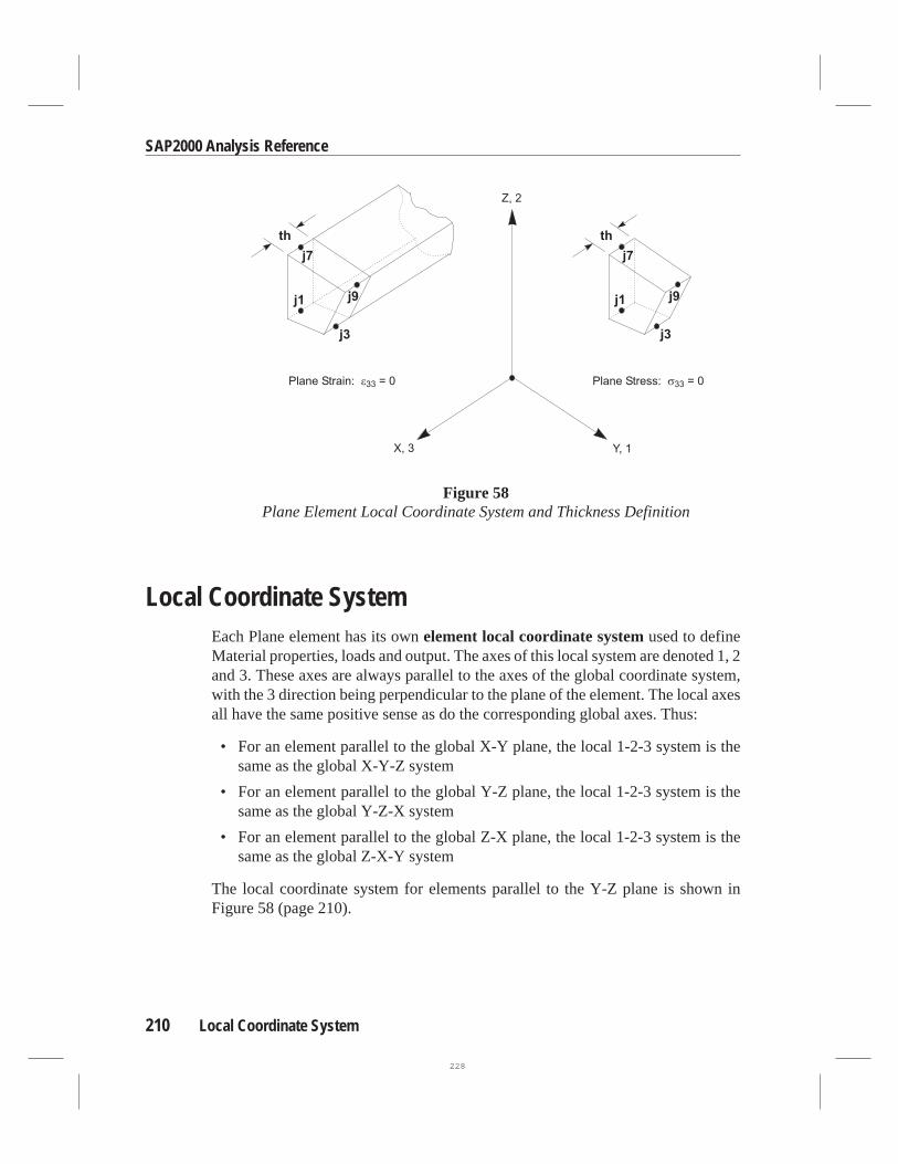
Local Coordinate SystemEach Plane element has its ownelement local coordinate systemused to defineMaterial properties, loads and output. The axes of this local system are denoted 1, 2and 3. These axes are always parallel to the axes of the global coordinate system,with the 3 direction being perpendicular to the plane of the element. The local axesall have the same positive sense as do the corresponding global axes. Thus:
• For an element parallel to the global X-Y plane, the local 1-2-3 system is thesame as the global X-Y-Z system
• For an element parallel to the global Y-Z plane, the local 1-2-3 system is thesame as the global Y-Z-X system
• For an element parallel to the global Z-X plane, the local 1-2-3 system is thesame as the global Z-X-Y system
The local coordinate system for elements parallel to the Y-Z plane is shown inFigure 58 (page 210).
210 Local Coordinate System
SAP2000 Analysis Reference
Figure 58Plane Element Local Coordinate System and Thickness Definition
228

Stresses and StrainsThe Plane element models the mid-plane of a structure having uniform thickness,and whose stresses and strains do not vary in the thickness direction.
Transverse shear stresses (σ12
, σ13
) and shear strains (γ12
, γ13
) are assumed to bezero. Displacements in the thickness (local 3) direction have no effect on the ele-ment.
Plane-stressis appropriate for structures that arethin compared to their planar di-mensions. The thickness normal stress (σ
33) is assumed to be zero. The thickness
normal strain (ε33
) may not be zero due to Poisson effects.
Plane-strainis appropriate for structures that arethickcompared to their planar di-mensions. The thickness normal strain (ε
33) is assumed to be zero. The thickness
normal stress (σ33
) may not be zero due to Poisson effects.
See Topic “Stresses and Strains” (page 137) in Chapter “Material Properties” formore information.
Material PropertiesThe material properties for each Plane element are specified by reference to apreviously-defined Material. Orthotropic properties are used, even if the Materialselected was defined as anisotropic. The material properties used by the Plane ele-ment are:
• The moduli of elasticity,e1, e2, ande3
• The shear modulus,g12
• The Poisson’s ratios,u12, u13andu23
• The coefficients of thermal expansion,a1, a2, anda3
• The mass density,m, for computing element mass
• The weight density,w, for computing Self-Weight and Gravity Loads
The propertiese3, u13, u23, anda3are not used for plane stress. They are used tocompute the thickness-normal stress (σ
33) in plane strain.
All material properties (except the densities) are obtained at the material tempera-ture of each individual element.
See Chapter “Material Properties” (page 135) for more information.
Stresses and Strains 211
Chapter XI The Plane Element
229

Material AngleThe material local coordinate system and the element local coordinate system neednot be the same. The local 3 directions always coincide for the two systems, but thematerial 1 axis and the element 1 axis may differ by the anglea as shown in Figure59 (page 212). This angle has no effect for isotropic material properties since theyare independent of orientation.
See Topic “Local Coordinate System” (page 136) in Chapter “Material Properties”for more information.
ThicknessEach element has a uniform thickness,th. This may be the actual thickness, particu-larly for plane-stress elements; or it may be a representative portion, such as a unitthickness of an infinitely-thick plane-strain element. See Figure 58 (page 210).
The element thickness is used for calculating the element stiffness, mass, and loads.Hence, joint forces computed from the element are proportional to this thickness.
212 Material Angle
SAP2000 Analysis Reference
Figure 59Plane Element Material Angle
230

MassIn a dynamic analysis, the mass of the structure is used to compute inertial forces.The mass contributed by the Plane element is lumped at the element joints.No iner-tial effects are considered within the element itself.
The total mass of the element is equal to the integral over the plane of the element ofthe mass density,m, multiplied by the thickness,th. The total mass is apportionedto the joints in a manner that is proportional to the diagonal terms of the consistentmass matrix. See Cook, Malkus, and Plesha (1989) for more information. The totalmass is applied to each of the three translational degrees of freedom (UX, UY, andUZ) even though the element contributes stiffness to only two of these degrees offreedom.
For more information:
• See Topic “Mass Density” (page 142) in Chapter “Material Properties.”
• See Chapter “Static and Dynamic Analysis” (page 291).
Self-Weight LoadSelf-Weight Load activates the self-weight of all elements in the model. For a Planeelement, the self-weight is a force that is uniformly distributed over the plane of theelement. The magnitude of the self-weight is equal to the weight density,w, multi-plied by the thickness,th.
Self-Weight Load always acts downward, in the global –Z direction. You may scalethe self-weight by a single scale factor that applies equally to all elements in thestructure.
For more information:
• See Topic “Weight Density” (page 143) in Chapter “Material Properties” forthe definition ofw.
• See Topic “Thickness” (page 212) in this chapter for the definition ofth.
• See Topic “Self-Weight Load” (page 283) in Chapter “Load Cases.”
Mass 213
Chapter XI The Plane Element
231

Gravity LoadGravity Load can be applied to each Plane element to activate the self-weight of theelement. Using Gravity Load, the self-weight can be scaled and applied in any di-rection. Different scale factors and directions can be applied to each element.
If all elements are to be loaded equally and in the downward direction, it is moreconvenient to use Self-Weight Load.
For more information:
• See Topic “Self-Weight Load” (page 213) in this chapter for the definition ofself-weight for the Plane element.
• See Topic “Gravity Load” (page 284) in Chapter “Load Cases.”
Surface Pressure LoadThe Surface Pressure Load is used to apply external pressure loads upon any of thethree or four side faces of the Plane element. The definition of these faces is shownin Figure 56 (page 207). Surface pressure always acts normal to the face. Positivepressures are directed toward the interior of the element.
The pressure may be constant over a face or interpolated from values given at thejoints. The values given at the joints are obtained from Joint Patterns, and need notbe the same for the different faces. Joint Patterns can be used to easily apply hydro-static pressures.
The pressure acting on a side is multiplied by the thickness,th, integrated along thelength of the side, and apportioned to the two or three joints on that side.
See Chapter “Load Cases” (page 279) for more information.
Pore Pressure LoadThe Pore Pressure Load is used to model the drag and buoyancy effects of a fluidwithina solid medium, such as the effect of water upon the solid skeleton of a soil.
Scalar fluid-pressure values are given at the element joints by Joint Patterns, and in-terpolated over the element. The total force acting on the element is the integral ofthe gradient of this pressure field over the plane of the element, multiplied by thethickness,th. This force is apportioned to each of the joints of the element. The
214 Gravity Load
SAP2000 Analysis Reference
232

forces are typically directed from regions of high pressure toward regions of lowpressure.
See Chapter “Load Cases” (page 279) for more information.
Temperature LoadThe Temperature Load creates thermal strain in the Plane element. This strain isgiven by the product of the Material coefficient of thermal expansion and the tem-perature change of the element. The temperature change is measured from the ele-ment Reference Temperature to the element Load Temperature. Temperaturechanges are assumed to be constant through the element thickness.
See Chapter “Load Cases” (page 279) for more information.
Stress OutputThe Plane element stresses are evaluated at the standard 2-by-2 Gauss integrationpoints of the element and extrapolated to the joints. See Cook, Malkus, and Plesha(1989) for more information.
The stresses are computed for the following types of Analysis Cases: Loads,Modes, Specs, Histories, and Combos. History results are the maximum and mini-mum values attained during the analysis, and are only available if specifically re-quested in the definition of the individual History cases. No results are available forMoving Loads or Combos that contain Moving Loads.
Principal values and their associated principal directions in the element local 1-2plane are also computed for the Loads and Modes. The angle given is measuredcounterclockwise (when viewed from the +3 direction) from the local 1 axis to thedirection of the maximum principal value.
It is important to note that the Response Spectrum results are always positive, andthat the correspondence between different values has been lost.
Plane element stresses are printed in the output file under the heading:
PLANE ELEMENT STRESSES
All results for a single element are printed together. Elements are presented inalpha-numeric order. For each Analysis Case the stresses are printed at all elementjoints.
Temperature Load 215
Chapter XI The Plane Element
233

The stresses are labeled S11, S22, S33, and S12 corresponding toσ11
, σ22
, σ33
,andσ
12, respectively, in the element local coordinate system. Stressesσ
12andσ
13
are always zero and are not printed.
Typical Plane element output is shown in Figure 60 (page 217).
By default, no stresses are printed. You may specify which Analysis Cases are to beprinted. The stresses can always be displayed using the SAP2000 graphical inter-face even if no results have been selected for printing.
For more information:
• See Chapter “Load Cases” (page 279).
• See Chapter “Static and Dynamic Analysis” (page 291).
• See Chapter “The Output Files” (page 395).
Joint Force OutputThePlane element joint forcesare concentrated forces acting at the joints of theelement that represent the effect of the rest of the structure upon the element.
See Topic “Element Joint Force Output” (page 402) in Chapter “The Output Files”for more information.
216 Joint Force Output
SAP2000 Analysis Reference
234

Joint Force Output 217
Chapter XI The Plane Element
P L A N E E L E M E N T S T R E S S E S
ELEM 1 ================== TYPE = PLANE STRESS
LOAD 1 ------------------
JOINT S11 S22 S33 S121 20.255067 0.465601 .000000 -13.8888892 83.333333 -0.409666 .000000 -13.8888893 146.411600 -1.284933 .000000 -13.8888896 4.09E-12 -4.70E-13 .000000 -13.8888897 2.35E-12 2.63E-12 .000000 -13.8888898 6.06E-13 5.72E-12 .000000 -13.888889
11 -20.255067 -0.465601 .000000 -13.88888912 -83.333333 0.409666 .000000 -13.88888913 -146.411600 1.284933 .000000 -13.888889
JOINT S-MAX S-MIN ANGLE1 27.413397 -6.692729 -27.2665702 85.576726 -2.653058 -9.1754113 147.706315 -2.579648 -5.3256936 13.888889 -13.888889 -45.0000007 13.888889 -13.888889 -45.0000008 13.888889 -13.888889 -45.000000
11 6.692729 -27.413397 -62.73343012 2.653058 -85.576726 -80.82458913 2.579648 -147.706315 -84.674307
ELEM 2 ================== TYPE = PLANE STRESS
LOAD 1 ------------------
JOINT S11 S22 S33 S1216 20.255067 0.465601 .000000 -13.88888917 83.333333 -0.409666 .000000 -13.88888918 146.411600 -1.284933 .000000 -13.88888921 4.09E-12 -4.70E-13 .000000 -13.88888922 2.35E-12 2.63E-12 .000000 -13.88888923 6.06E-13 5.72E-12 .000000 -13.88888926 -20.255067 -0.465601 .000000 -13.88888927 -83.333333 0.409666 .000000 -13.88888928 -146.411600 1.284933 .000000 -13.888889
JOINT S-MAX S-MIN ANGLE16 27.413397 -6.692729 -27.26657017 85.576726 -2.653058 -9.17541118 147.706315 -2.579648 -5.32569321 13.888889 -13.888889 -45.00000022 13.888889 -13.888889 -45.00000023 13.888889 -13.888889 -45.00000026 6.692729 -27.413397 -62.73343027 2.653058 -85.576726 -80.82458928 2.579648 -147.706315 -84.674307
...Output Edited for Brevity...
Figure 60Plane Element Stresses in the Output File
235

218 Joint Force Output
SAP2000 Analysis Reference
236

C h a p t e r XII
The Asolid Element
TheAsolid element is used to model axisymmetric solids under axisymmetric load-ing.
Advanced Topics
• Overview
• Joint Connectivity
• Degrees of Freedom
• Local Coordinate System
• Stresses and Strains
• Material Properties
• Material Angle
• Arc and Thickness
• Mass
• Self-Weight Load
• Gravity Load
• Surface Pressure Load
• Pore Pressure Load
219
237

• Temperature Load
• Rotate Load
• Stress Output
• Joint Force Output
OverviewThe Asolid element is a three- to nine-node element for modeling axisymmetricstructures under axisymmetric loading. It is based upon an isoparametric formula-tion (Hollings and Wilson, 1977).
The element models a representative two-dimensional cross section of the three-dimensional axisymmetric solid. The axis of symmetry must be one of the globalaxes, and the element must exist in one of the global principal planes (in the X-Y,Y-Z, or Z-X planes).
The geometry, loading, displacements, stresses, and strains are assumed not to varyin the circumferential direction. Any displacements that occur in the circumferen-tial direction do not affect the element..
Each Asolid element has its own local coordinate system that is aligned with theglobal system. The local coordinate system is used for defining Material propertiesand loads, and for interpreting output.
Temperature-dependent, orthotropic material properties are allowed. Each elementmay be loaded by gravity (in any direction); centrifugal force; surface pressure onthe side faces; pore pressure within the element; and loads due to temperaturechange.
An eight-point numerical integration scheme is used for the Asolid. Stresses in theelement local coordinate system are evaluated at the integration points and extrapo-lated to the joints of the element. An approximate error in the stresses can be esti-mated from the difference in values calculated from different elements attached to acommon joint. This will give an indication of the accuracy of the finite element ap-proximation and can then be used as the basis for the selection of a new and moreaccurate finite element mesh.
The nine-node option is the recommended formulation.
220 Overview
SAP2000 Analysis Reference
238

Joint ConnectivityAll joints for a given element must lie in one of the principal global planes. The axisof symmetry and radial direction are as follows:
ElementPlane
RadialDirectionLocal 1
Axis ofSymmetry
Local 2
CircumferentialDirectionLocal 3
X-Y X Y Z
Y-Z Y Z X
Z-X Z X Y
The radial coordinate must not be negative for any of the element’s joints.
Each Asolid element may have either of the following shapes, as shown in Figure61 (page 222):
• Quadrilateral, defined by the four corner jointsj1, j3, j7, andj9, plus the op-tional midside jointsj2, j4, j6, andj8, and the optional center jointj5.
• Triangular, defined by the three jointsj1, j3, andj7 only.
The pathj1-j3-j7 mustappear counterclockwise when viewed from the positiveglobal coordinate direction that is perpendicular to the plane of the element, i.e.,when viewed from +Z, +X, or +Y, respectively, corresponding to the table above.
For the best accuracy, the use of the nine-node quadrilateral is recommended. How-ever, the variable node option of the element is very useful for generating transitioninterfaces between coarse and fine finite element meshes. See Figure 62 (page 223)for examples.
The locations of the joints should be chosen to meet the following geometric condi-tions:
• The inside angle at each corner must be less than 180°. Best results for thequadrilateral will be obtained when these angles are near 90°, or at least in therange of 45° to 135°.
• The aspect ratio of an element should not be too large. For the triangle, this isthe ratio of the longest side to the shortest side. For the quadrilateral, this is theratio of the longer distance between the midpoints of opposite sides to the
Joint Connectivity 221
Chapter XII The Asolid Element
239

shorter such distance. Best results are obtained for aspect ratios near unity, or atleast less than four. The aspect ratio should not exceed ten.
• If a midside joint is present, it should be near the center of the side, or at leastbetween the quarter points. Best results are obtained if the side is straight. If theside is curved, the distance from the midside joint to the straight line between
222 Joint Connectivity
SAP2000 Analysis Reference
Figure 61Asolid Element Joint Connectivity and Face Definitions
240

the corner joints should be no larger than half the distance between the cornerjoints.
• The position of the center joint with respect to each pair of opposite midsidejoints is subject to the same rules as is the position of a midside joint with re-spect to the corner joints.
Joint Connectivity 223
Chapter XII The Asolid Element
Figure 62Examples of Asolid Element Mesh Transitions
241

Asolid elements should not be connected to joints that are connected to other typesof elements unless special provisions are made to enforce axisymmetric conditionsupon these joints.
Degrees of FreedomThe Asolid element activates the three translational degrees of freedom at each ofits connected joints. Rotational degrees of freedom are not activated.
This element contributes stiffness only to the degrees of freedom in the plane of theelement. It is necessary to provide restraints or other supports for the translationaldegrees of freedom that are normal to this plane; otherwise, the structure will be un-stable.
See Topic “Degrees of Freedom” (page 83) in Chapter “Joints and Degrees of Free-dom” for more information.
Local Coordinate SystemEach Asolid element has its ownelement local coordinate systemused to defineMaterial properties, loads and output. The axes of this local system are denoted 1, 2and 3. These axes are always parallel to the axes of the global coordinate systemwith the same positive sense.
Local axis 1 is parallel to the radial direction, axis 2 is parallel to the axis of symme-try, and axis 3 is tangent to the circumferential direction of the axisymmetric solid.See the table in Topic “Joint Connectivity” (page 221). The local coordinate systemfor elements parallel to the Y-Z plane is shown in Figure 63 (page 225).
Stresses and StrainsThe Asolid element models the mid-plane of a representative sector of an axisym-metric structure whose stresses and strains do not vary in the circumferential direc-tion.
Circumferential shear stresses (σ12
,σ13
) and shear strains (γ12
, γ13
) are assumed tobe zero. Displacements in the circumferential (local 3) direction have no effect onthe element.
Displacements in the radial (local 1) direction cause circumferential normal strains:
224 Degrees of Freedom
SAP2000 Analysis Reference
242

ε33
1= u
r
whereu1 is the radial displacement, andr is the radius at the point in question.
The circumferential normal stress (σ33
) is computed as usual from the three normalstrains.
See Topic “Stresses and Strains” (page 137) in Chapter “Material Properties” formore information.
Material PropertiesThe material properties for each Asolid element are specified by reference to apreviously-defined Material. Orthotropic properties are used, even if the Materialselected was defined as anisotropic. The material properties used by the Asolid ele-ment are:
• The moduli of elasticity,e1, e2, ande3
• The shear modulus,g12
Material Properties 225
Chapter XII The Asolid Element
Figure 63Asolid Element Local Coordinate System and Arc Definition
243

• The Poisson’s ratios,u12, u13andu23
• The coefficients of thermal expansion,a1, a2, anda3
• The mass density,m, for computing element mass
• The weight density,w, for computing Self-Weight and Gravity Loads
All material properties (except the densities) are obtained at the material tempera-ture of each individual element.
See Chapter “Material Properties” (page 135) for more information.
Material AngleThe material local coordinate system and the element local coordinate system neednot be the same. The local 3 directions always coincide for the two systems, but thematerial 1 axis and the element 1 axis may differ by the anglea as shown in Figure64 (page 226). This angle has no effect for isotropic material properties since theyare independent of orientation.
226 Material Angle
SAP2000 Analysis Reference
Figure 64Asolid Element Material Angle
244

See Topic “Local Coordinate System” (page 136) in Chapter “Material Properties”for more information.
Arc and ThicknessThe Asolid element represents a solid that is created by rotating the element’s pla-nar shape through 360° about the axis of symmetry. However, the analysis consid-ers only a representative sector of the solid. You can specify the size of the sector, indegrees, using the parameterarc. For example,arc=360 models the full structure,andarc=90 models one quarter of it. See Figure 63 (page 225). Settingarc=0, thedefault, models a one-radian sector. One radian is the same as 180°/π, or approxi-mately 57.3°.
The element “thickness” (circumferential extent),h, increases with the radial dis-tance,r, from the axis of symmetry:
h r= ⋅π arc
180
Clearly the thickness varies over the plane of the element.
The element thickness is used for calculating the element stiffness, mass, and loads.Hence, joint forces computed from the element are proportional toarc.
MassIn a dynamic analysis, the mass of the structure is used to compute inertial forces.The mass contributed by the Asolid element is lumped at the element joints.No in-ertial effects are considered within the element itself.
The total mass of the element is equal to the integral over the plane of the element ofthe product of the mass density,m, multiplied by the thickness,h. The total mass isapportioned to the joints in a manner that is proportional to the diagonal terms of theconsistent mass matrix. See Cook, Malkus, and Plesha (1989) for more informa-tion. The total mass is applied to each of the three translational degrees of freedom(UX, UY, and UZ) even though the element contributes stiffness to only two ofthese degrees of freedom.
For more information:
• See Topic “Mass Density” (page 142) in Chapter “Material Properties.”
Arc and Thickness 227
Chapter XII The Asolid Element
245

• See Chapter “Static and Dynamic Analysis” (page 291).
Self-Weight LoadSelf-Weight Load activates the self-weight of all elements in the model. For anAsolid element, the self-weight is a force that is distributed over the plane of theelement. The magnitude of the self-weight is equal to the weight density,w, multi-plied by the thickness,h.
Self-Weight Load always acts downward, in the global –Z direction. If the down-ward direction corresponds to the radial or circumferential direction of an Asolidelement, the Self-Weight Load for that element will be zero, since self-weight act-ing in these directions is not axisymmetric. Non-zero Self-Weight Load will onlyexist for elements whose axial (local 2) direction is vertical.
You may scale the self-weight by a single scale factor that applies equally to all ele-ments in the structure.
For more information:
• See Topic “Weight Density” (page 143) in Chapter “Material Properties” forthe definition ofw.
• See Topic “Arc and Thickness” (page 227) in this chapter for the definition ofh.
• See Topic “Self-Weight Load” (page 283) in Chapter “Load Cases.”
Gravity LoadGravity Load can be applied to each Asolid element to activate the self-weight ofthe element. Using Gravity Load, the self-weight can be scaled and applied in anydirection. Different scale factors and directions can be applied to each element.However, only the components of Gravity load acting in the axial direction of anAsolid element will be non-zero. Components in the radial or circumferential direc-tion will be set to zero, since gravity acting in these directions is not axisymmetric.
If all elements are to be loaded equally and in the downward direction, it is moreconvenient to use Self-Weight Load.
For more information:
228 Self-Weight Load
SAP2000 Analysis Reference
246

• See Topic “Self-Weight Load” (page 228) in this chapter for the definition ofself-weight for the Asolid element.
• See Topic “Gravity Load” (page 284) in Chapter “Load Cases.”
Surface Pressure LoadThe Surface Pressure Load is used to apply external pressure loads upon any of thethree or four side faces of the Asolid element. The definition of these faces is shownin Figure 61 (page 222). Surface pressure always acts normal to the face. Positivepressures are directed toward the interior of the element.
The pressure may be constant over a face or interpolated from values given at thejoints. The values given at the joints are obtained from Joint Patterns, and need notbe the same for the different faces. Joint Patterns can be used to easily apply hydro-static pressures.
The pressure acting on a side is multiplied by the thickness,h, integrated along thelength of the side, and apportioned to the two or three joints on that side.
See Chapter “Load Cases” (page 279) for more information.
Pore Pressure LoadThe Pore Pressure Load is used to model the drag and buoyancy effects of a fluidwithina solid medium, such as the effect of water upon the solid skeleton of a soil.
Scalar fluid-pressure values are given at the element joints by Joint Patterns, and in-terpolated over the element. The total force acting on the element is the integral ofthe gradient of this pressure field, multiplied by the thicknessh, over the plane ofthe element. This force is apportioned to each of the joints of the element. Theforces are typically directed from regions of high pressure toward regions of lowpressure.
See Chapter “Load Cases” (page 279) for more information.
Temperature LoadThe Temperature Load creates thermal strain in the Asolid element. This strain isgiven by the product of the Material coefficient of thermal expansion and the tem-perature change of the element. The temperature change is measured from the ele-
Surface Pressure Load 229
Chapter XII The Asolid Element
247

ment Reference Temperature to the element Load Temperature. Temperaturechanges are assumed to be constant through the element thickness.
See Chapter “Load Cases” (page 279) for more information.
Rotate LoadRotate Load is used to apply centrifugal force to Asolid elements. Each element isassumed to rotate about its own axis of symmetry at a constant angular velocity.
The angular velocity creates a load on the element that is proportional to its mass,its distance from the axis of rotation, and the square of the angular velocity. Thisload acts in the positive radial direction, and is apportioned to each joint of the ele-ment. No Rotate Load will be produced by an element with zero mass density.
Since Rotate Loads assume a constant rate of rotation, it does not make sense to usea Load Case that contains Rotate Load in a time-history analysis unless that LoadCase is applied quasi-statically (i.e., with avery slowtime variation).
For more information:
• See Topic “Mass Density” (page 142) in Chapter “Material Properties.”
• See Chapter “Load Cases” (page 279).
Stress OutputThe Asolid element stresses are evaluated at the standard 2-by-2 Gauss integrationpoints of the element and extrapolated to the joints. See Cook, Malkus, and Plesha(1989) for more information.
The stresses are computed for the following types of Analysis Cases: Loads,Modes, Specs, Histories, and Combos. History results are the maximum and mini-mum values attained during the analysis, and are only available if specifically re-quested in the definition of the individual History cases. No results are available forMoving Loads or Combos that contain Moving Loads.
Principal values and their associated principal directions in the element local 1-2plane are also computed for the Loads and Modes. The angle given is measuredcounterclockwise (when viewed from the +3 direction) from the local 1 axis to thedirection of the maximum principal value.
230 Rotate Load
SAP2000 Analysis Reference
248

It is important to note that the Response Spectrum results are always positive, andthat the correspondence between different values has been lost.
Asolid element stresses are printed in the output file under the heading:
ASOLID ELEMENT STRESSES
All results for a single element are printed together. Elements are presented inalpha-numeric order. For each Analysis Case the stresses are printed at all elementjoints.
The stresses are labeled S11, S22, S33, and S12 corresponding toσ11
, σ22
, σ33
,andσ
12, respectively, in the element local coordinate system. Stressesσ
12andσ
13
are always zero and are not printed.
Typical Asolid element output is shown in Figure 65 (page 232).
By default, no stresses are printed. You may specify which Analysis Cases are to beprinted. The stresses can always be displayed using the SAP2000 graphical inter-face even if no results have been selected for printing.
For more information:
• See Chapter “Load Cases” (page 279).
• See Chapter “Static and Dynamic Analysis” (page 291).
• See Chapter “The Output Files” (page 395).
Joint Force OutputTheAsolid element joint forcesare concentrated forces acting at the joints of theelement that represent the effect of the rest of the structure upon the element.
See Topic “Element Joint Force Output” (page 402) in Chapter “The Output Files”for more information.
Joint Force Output 231
Chapter XII The Asolid Element
249

232 Joint Force Output
SAP2000 Analysis Reference
A S O L I D E L E M E N T S T R E S S E S
ELEM 1 ==================
LOAD INTPRES ------------------
JOINT S11 S22 S33 S121 -0.939522 0.157629 1.255412 0.0009202 -0.836460 0.114523 1.065966 0.0008293 -0.733398 0.071418 0.876520 0.000739
12 -0.939522 0.157629 1.255412 -2.89E-1313 -0.836460 0.114523 1.065966 -2.32E-1314 -0.733398 0.071418 0.876520 -1.76E-1323 -0.939522 0.157629 1.255412 -0.00092024 -0.836460 0.114523 1.065966 -0.00082925 -0.733398 0.071418 0.876520 -0.000739
JOINT S-MAX S-MIN ANGLE1 0.157630 -0.939523 89.9519472 0.114524 -0.836461 89.9500333 0.071418 -0.733399 89.947423
12 0.157629 -0.939522 -90.00000013 0.114523 -0.836460 -90.00000014 0.071418 -0.733398 -90.00000023 0.157630 -0.939523 -89.95194724 0.114524 -0.836461 -89.95003325 0.071418 -0.733399 -89.947423
LOAD LOGTEMP ------------------
JOINT S11 S22 S33 S121 -9.421631 -172.393810 -136.017533 -0.1878452 -9.169759 -150.661663 -106.777127 -0.1729323 -8.917887 -128.929517 -77.536722 -0.158019
12 -9.421631 -172.393810 -136.017533 -1.28E-1113 -9.169759 -150.661663 -106.777127 -9.82E-1214 -8.917887 -128.929517 -77.536722 -6.79E-1223 -9.421631 -172.393810 -136.017533 0.18784524 -9.169759 -150.661663 -106.777127 0.17293225 -8.917887 -128.929517 -77.536722 0.158019
ELEM 2 ==================
LOAD INTPRES ------------------
JOINT S11 S22 S33 S123 -0.634081 0.168448 0.971652 0.0006814 -0.561526 0.117673 0.797344 0.0006135 -0.488971 0.066898 0.623036 0.000545
14 -0.634081 0.168448 0.971652 -1.46E-1315 -0.561526 0.117673 0.797344 -2.06E-1416 -0.488971 0.066898 0.623036 1.05E-1325 -0.634081 0.168448 0.971652 -0.00068126 -0.561526 0.117673 0.797344 -0.00061327 -0.488971 0.066898 0.623036 -0.000545
...Output Edited for Brevity...
Figure 65Asolid Element Stresses in the Output File
250

C h a p t e r XIII
The Solid Element
TheSolid element is used to model three-dimensional solid structures.
Advanced Topics
• Overview
• Joint Connectivity
• Degrees of Freedom
• Local Coordinate System
• Stresses and Strains
• Material Properties
• Material Angles
• Incompatible Bending Modes
• Mass
• Self-Weight Load
• Gravity Load
• Surface Pressure Load
• Pore Pressure Load
• Temperature Load
233
251

• Stress Output
• Joint Force Output
OverviewThe Solid element is an eight-node element for modeling three-dimensional struc-tures and solids. It is based upon an isoparametric formulation that includes nineoptional incompatible bending modes.
The incompatible bending modes significantly improve the bending behavior of theelement if the element geometry is of a rectangular form. Improved behavior is ex-hibited even with non-rectangular geometry.
The local coordinate system for each Solid element is identical to the global system.The local coordinate system is used for defining Material properties and loads, andfor interpreting output.
Temperature-dependent, anisotropic material properties are allowed. Each elementmay be loaded by gravity (in any direction); surface pressure on the faces; porepressure within the element; and loads due to temperature change.
An 2 x 2 x 2numerical integration scheme is used for the Solid. Stresses in the ele-ment local coordinate system are evaluated at the integration points and extrapo-lated to the joints of the element. An approximate error in the stresses can be esti-mated from the difference in values calculated from different elements attached to acommon joint. This will give an indication of the accuracy of the finite element ap-proximation and can then be used as the basis for the selection of a new and moreaccurate finite element mesh.
Joint ConnectivityEach Solid element has six quadrilateral faces, with a joint located at each of theeight corners as shown in Figure 66 (page 235). It is important to note the relativeposition of the eight joints: the pathsj1-j2-j3 andj5-j6-j7 should appear counter-clockwise when viewed along the direction fromj5 to j1. Mathematically stated,the three vectors:
• V12
, from jointsj1 to j2,
• V13
, from jointsj1 to j3,
234 Overview
SAP2000 Analysis Reference
252

• V15
, from jointsj1 to j5,
must form a positive triple product, that is:
( )V V V12 13 15
0× ⋅ >
The locations of the joints should be chosen to meet the following geometric condi-tions:
• The inside angle at each corner of the faces must be less than 180°. Best resultswill be obtained when these angles are near 90°, or at least in the range of 45° to135°.
• The aspect ratio of an element should not be too large. This is the ratio of thelongest dimension of the element to its shortest dimension. Best results are ob-tained for aspect ratios near unity, or at least less than four. The aspect ratioshould not exceed ten.
These conditions can usually be met with adequate mesh refinement.
Joint Connectivity 235
Chapter XIII The Solid Element
Figure 66Solid Element Joint Connectivity and Face Definitions
253

Degrees of FreedomThe Solid element activates the three translational degrees of freedom at each of itsconnected joints. Rotational degrees of freedom are not activated. This elementcontributes stiffness to all of these translational degrees of freedom.
See Topic “Degrees of Freedom” (page 83) in Chapter “Joints and Degrees of Free-dom” for more information.
Local Coordinate SystemEach Solid element has its ownelement local coordinate systemused to defineMaterial properties, loads and output. The axes of this local system are denoted 1, 2and 3. These axesalwayscorrespond with the global coordinate axes X, Y and Z,respectively, regardless of the orientation of the element.
Stresses and StrainsThe Solid element models a general state of stress and strain in a three-dimensionalsolid. All six stress and strain components are active for this element.
See Topic “Stresses and Strains” (page 137) in Chapter “Material Properties” formore information.
Material PropertiesThe material properties for each Solid element are specified by reference to apreviously-defined Material. Fully anisotropic material properties are used. Thematerial properties used by the Solid element are:
• The moduli of elasticity,e1, e2, ande3
• The shear moduli,g12, g13, andg23
• All of the Poisson’s ratios,u12, u13, u23, ...,u56
• The coefficients of thermal expansion,a1, a2, a3, a12, a13, anda23
• The mass density,m, used for computing element mass
• The weight density,w, used for computing Self-Weight and Gravity Loads
236 Degrees of Freedom
SAP2000 Analysis Reference
254

All material properties (except the densities) are obtained at the material tempera-ture of each individual element.
See Chapter “Material Properties” (page 135) for more information.
Material AnglesThe material local coordinate system and the element local coordinate system neednot be the same. The material coordinate system is oriented with respect to the ele-ment coordinate system using the three anglesa, b, andcaccording to the followingprocedure:
• The material system is first aligned with the element system;
• The material system is then rotated about its +3 axis by anglea;
• The material system is next rotated about the resulting +2 axis by angleb;
• The material system is lastly rotated about the resulting +1 axis by anglec;
This is shown in Figure 67 (page 238). These angles have no effect for isotropic ma-terial properties since they are independent of orientation.
See Topic “Local Coordinate System” (page 136) in Chapter “Material Properties”for more information.
Incompatible Bending ModesBy default each Solid element includes nine incompatible bending modes in itsstiffness formulation. These incompatible bending modes significantly improve thebending behavior of the element if the element geometry is of a rectangular form.Improved behavior is exhibited even with non-rectangular geometry.
If an element is severely distorted, the inclusion of the incompatible modes shouldbe suppressed. The element then uses the standard isoparametric formulation. In-compatible bending modes may also be suppressed in cases where bending is notimportant, such as in typical geotechnical problems.
Material Angles 237
Chapter XIII The Solid Element
255

MassIn a dynamic analysis, the mass of the structure is used to compute inertial forces.The mass contributed by the Solid element is lumped at the element joints.No iner-tial effects are considered within the element itself.
The total mass of the element is equal to the integral of the mass density,m, over thevolume of the element. The total mass is apportioned to the joints in a manner that isproportional to the diagonal terms of the consistent mass matrix. See Cook,Malkus, and Plesha (1989) for more information. The total mass is applied to eachof the three translational degrees of freedom (UX, UY, and UZ).
For more information:
• See Topic “Mass Density” (page 142) in Chapter “Material Properties.”
• See Chapter “Static and Dynamic Analysis” (page 291).
238 Mass
SAP2000 Analysis Reference
Figure 67Solid Element Material Angles
256

Self-Weight LoadSelf-Weight Load activates the self-weight of all elements in the model. For a Solidelement, the self-weight is a force that is uniformly distributed over the volume ofthe element. The magnitude of the self-weight is equal to the weight density,w.
Self-Weight Load always acts downward, in the global –Z direction. You may scalethe self-weight by a single scale factor that applies equally to all elements in thestructure.
For more information:
• See Topic “Weight Density” (page 143) in Chapter “Material Properties” forthe definition ofw.
• See Topic “Self-Weight Load” (page 283) in Chapter “Load Cases.”
Gravity LoadGravity Load can be applied to each Solid element to activate the self-weight of theelement. Using Gravity Load, the self-weight can be scaled and applied in any di-rection. Different scale factors and directions can be applied to each element.
If all elements are to be loaded equally and in the downward direction, it is moreconvenient to use Self-Weight Load.
For more information:
• See Topic “Self-Weight Load” (page 239) in this chapter for the definition ofself-weight for the Solid element.
• See Topic “Gravity Load” (page 284) in Chapter “Load Cases.”
Surface Pressure LoadThe Surface Pressure Load is used to apply external pressure loads upon any of thesix faces of the Solid element. The definition of these faces is shown in Figure 66(page 235). Surface pressure always acts normal to the face. Positive pressures aredirected toward the interior of the element.
The pressure may be constant over a face or interpolated from values given at thejoints. The values given at the joints are obtained from Joint Patterns, and need not
Self-Weight Load 239
Chapter XIII The Solid Element
257

be the same for the different faces. Joint Patterns can be used to easily apply hydro-static pressures.
The pressure acting on a given face is integrated over the area of that face, and theresulting force is apportioned to the four corner joints of the face.
See Chapter “Load Cases” (page 279) for more information.
Pore Pressure LoadThe Pore Pressure Load is used to model the drag and buoyancy effects of a fluidwithina solid medium, such as the effect of water upon the solid skeleton of a soil.
Scalar fluid-pressure values are given at the element joints by Joint Patterns, and in-terpolated over the element. The total force acting on the element is the integral ofthe gradient of this pressure field over the volume of the element. This force is ap-portioned to each of the joints of the element. The forces are typically directed fromregions of high pressure toward regions of low pressure.
See Chapter “Load Cases” (page 279) for more information.
Temperature LoadThe Temperature Load creates thermal strain in the Solid element. This strain isgiven by the product of the Material coefficient of thermal expansion and the tem-perature change of the element. The temperature change is measured from the ele-ment Reference Temperature to the element Load Temperature. Temperaturechanges are assumed to be constant through the element thickness.
See Chapter “Load Cases” (page 279) for more information.
Stress OutputThe Solid element stresses are evaluated at the standard 2 x 2 x 2Gauss integrationpoints of the element and extrapolated to the joints. See Cook, Malkus, and Plesha(1989) for more information.
The stresses are computed for the following types of Analysis Cases: Loads,Modes, Specs, Histories, and Combos. History results are the maximum and mini-mum values attained during the analysis, and are only available if specifically re-
240 Pore Pressure Load
SAP2000 Analysis Reference
258

quested in the definition of the individual History cases. No results are available forMoving Loads or Combos that contain Moving Loads.
Principal values and their associated principal directions in the element local coor-dinate system are also computed for the Loads and Modes. Three direction cosineseach are given for the directions of the maximum and minimum principal stresses.The direction of the middle principal stress is perpendicular to the maximum andminimum principal directions.
It is important to note that the Response Spectrum results are always positive, andthat the correspondence between different values has been lost.
Solid element stresses are printed in the output file under the heading:
SOLID ELEMENT STRESSES
All results for a single element are printed together. Elements are presented inalpha-numeric order. For each Analysis Case the stresses are printed at all elementjoints.
The stresses are labeled S11, S22, S33, S12, S13, and S23 corresponding toσ11
,σ
22, σ
33, σ
12, σ
13, andσ
23, respectively, in the element local coordinate system.
Typical Solid element output is shown in Figure 68 (page 242).
By default, no stresses are printed. You may specify which Analysis Cases are to beprinted. The stresses can always be displayed using the SAP2000 graphical inter-face even if no results have been selected for printing.
For more information:
• See Chapter “Load Cases” (page 279).
• See Chapter “Static and Dynamic Analysis” (page 291).
• See Chapter “The Output Files” (page 395).
Joint Force OutputTheSolid element joint forcesare concentrated forces acting at the joints of theelement that represent the effect of the rest of the structure upon the element.
See Topic “Element Joint Force Output” (page 402) in Chapter “The Output Files”for more information.
Joint Force Output 241
Chapter XIII The Solid Element
259

242 Joint Force Output
SAP2000 Analysis Reference
S O L I D E L E M E N T S T R E S S E S
ELEM 1 ==================
LOAD 1 ------------------
JOINT S11 S22 S33 S12 S13 S233 -0.364752 207.803651 6.559145 -0.247394 -0.494788 -13.888889
18 -0.364752 207.803651 6.559145 0.247394 0.494788 -13.8888894 -0.199823 208.298440 -3.171692 -0.247394 0.494788 -13.888889
19 -0.199823 208.298440 -3.171692 0.247394 -0.494788 -13.8888898 1.966476 0.811970 7.053933 0.247394 -0.494788 -13.888889
23 1.966476 0.811970 7.053933 -0.247394 0.494788 -13.8888899 -0.837325 0.317181 -3.666480 0.247394 0.494788 -13.888889
24 -0.837325 0.317181 -3.666480 -0.247394 -0.494788 -13.888889
JOINT S-MAX S-MID S-MIN MAX-1 MAX-2 MAX-3 MIN-1 MIN-2 MIN-33 208.757887 5.648477 -0.408320 -.001 .998 -.069 .996 .007 .084
18 208.757887 5.648477 -0.408320 .001 .998 -.069 .996 -.007 -.0844 209.207102 -0.142270 -4.137907 -.001 .998 -.065 -.120 .065 .991
19 209.207102 -0.142270 -4.137907 .001 .998 -.065 .120 .065 .9918 18.186219 1.949535 -10.303376 -.033 -.624 .780 .009 .781 .625
23 18.186219 1.949535 -10.303376 .033 -.624 .780 -.009 .781 .6259 12.357765 -0.819458 -15.724930 -.010 .755 -.655 -.036 .654 .755
24 12.357765 -0.819458 -15.724930 .010 .755 -.655 .036 .654 .755
ELEM 2 ==================
LOAD 1 ------------------
JOINT S11 S22 S33 S12 S13 S238 -1.966476 -0.811970 -7.053933 -0.247394 -0.494788 -13.888889
23 -1.966476 -0.811970 -7.053933 0.247394 0.494788 -13.8888899 0.837325 -0.317181 3.666480 -0.247394 0.494788 -13.888889
24 0.837325 -0.317181 3.666480 0.247394 -0.494788 -13.88888913 0.364752 -207.803651 -6.559145 0.247394 -0.494788 -13.88888928 0.364752 -207.803651 -6.559145 -0.247394 0.494788 -13.88888914 0.199823 -208.298440 3.171692 0.247394 0.494788 -13.88888929 0.199823 -208.298440 3.171692 -0.247394 -0.494788 -13.888889
JOINT S-MAX S-MID S-MIN MAX-1 MAX-2 MAX-3 MIN-1 MIN-2 MIN-38 10.303376 -1.949535 -18.186219 .009 .781 -.625 .033 .624 .780
23 10.303376 -1.949535 -18.186219 -.009 .781 -.625 -.033 .624 .7809 15.724930 0.819458 -12.357765 .036 -.654 .755 -.010 .755 .655
24 15.724930 0.819458 -12.357765 -.036 -.654 .755 .010 .755 .65513 0.408320 -5.648477 -208.757887 .996 .007 -.084 -.001 .998 .06928 0.408320 -5.648477 -208.757887 .996 -.007 .084 .001 .998 .06914 4.137907 0.142270 -209.207102 .120 -.065 .991 -.001 .998 .06529 4.137907 0.142270 -209.207102 -.120 -.065 .991 .001 .998 .065
...Output Edited for Brevity...
Figure 68Solid Element Stresses in the Output File
260

C h a p t e r XIV
The Nllink Element
TheNllink element is used to model local structural nonlinearities such as gaps,dampers, isolators, and the like. Nonlinear behavior is exhibited only during non-linear time-history analyses. For all other analyses, the Nllink element behaveslinearly.
Advanced Topics
• Overview
• Joint Connectivity
• Zero-Length Elements
• Degrees of Freedom
• Local Coordinate System
• Advanced Local Coordinate System
• Internal Deformations
• Nlprop Properties
• Nonlinear Deformation Loads
• Mass
• Self-Weight Load
243
261

• Gravity Load
• Internal Force and Deformation Output
• Joint Force Output
OverviewTheNllink element is used to model local structural nonlinearities.Nonlinear be-havior is only exhibited during nonlinear time-history analyses. For all otheranalyses, the Nllink element behaves linearly.
Each Nllink element may be either a one-joint grounded spring or a two-joint link.Properties for either type of element are defined in the same way.
Each element is assumed to be composed of six separate “springs,” one for each ofsix deformational degrees-of freedom (axial, shear, torsion, and pure bending).Each of these springs possesses a dual set of properties:
• Linear effective-stiffness and effective-damping properties used for all linearanalyses
• An optional nonlinear force-deformation relationship used only for nonlineartime-history analyses
If the optional nonlinear properties are not specified for a given degree of freedom,the linear stiffness (but not damping) properties are used for nonlinear time-historyanalyses.
The linear effective damping property is only used for response-spectrum analysesand linear time-history analyses.
The nonlinear force-deformation relationships of these springs may be coupled oruncoupled, depending on the type of behavior modeled.
A set of properties for all six degrees of freedom is called an Nlprop. Each Nlpropconsists of mass, weight, and up to six linear and nonlinear force-deformation rela-tionships that may be used by one or more Nllink elements.
The types of nonlinear behavior that can be modeled with this element include:
• Viscoelastic damping
• Gap (compression only) and hook (tension only)
• Uniaxial plasticity
244 Overview
SAP2000 Analysis Reference
262

• Biaxial-plasticity base isolator
• Friction-pendulum base isolator
Each element has its own local coordinate system for defining the force-deformation properties and for interpreting output.
Each Nllink element may be loaded by gravity (in any direction).
Available output includes the deformation across the element, and the internalforces at the joints of the element.
Joint ConnectivityEach Nllink element may take one of the following two configurations:
• A link connecting two joints,i andj ; it is permissible for the two joints to sharethe same location in space
• A spring connecting a single joint,j , to ground
Zero-Length ElementsThe following types of Nllink elements are considered to be ofzero length:
• Single-joint elements
• Two-joint elements with the distance from jointi to joint j being less than orequal to the zero-length tolerance,zero, that you specify.
The default value forzero is 10-3. The purpose of this tolerance is to account for nu-merical round-off in the specification and generation of joint coordinates. For ex-ample, if joint coordinates are specified to the nearest millimeter, then a possiblevalue forzeromight be 2 or 3 mm.
Two-joint elements having a length greater than the tolerancezeroare consideredto be of finite length. Whether an element is of zero length or finite length affectsthe definition of the element local coordinate system.
Joint Connectivity 245
Chapter XIV The Nllink Element
263

Degrees of FreedomThe Nllink element always activates all six degrees of freedom at its one or twoconnected joints. To which joint degrees of freedom the element contributes stiff-ness depends upon the properties you assign to the element. You must ensure thatrestraints or other supports are provided to those joint degrees of freedom that re-ceive no stiffness.
For more information:
• See Topic “Degrees of Freedom” (page 83) in Chapter “Joints and Degrees ofFreedom.”
• See Topic “Nlprop Properties” (page 254) in this chapter.
Local Coordinate SystemEach Nllink element has its ownelement local coordinate systemused to defineforce-deformation properties and output. The axes of this local system are denoted1, 2 and 3. The first axis is directed along the length of the element and correspondsto extensional deformation. The remaining two axes lie in the plane perpendicularto the element and have an orientation that you specify; these directions correspondto shear deformation.
It is important that you clearly understand the definition of the element local 1-2-3coordinate system and its relationship to the global X-Y-Z coordinate system. Bothsystems are right-handed coordinate systems. It is up to you to define local systemswhich simplify data input and interpretation of results.
In most structures the definition of the element local coordinate system is extremelysimple. The methods provided, however, provide sufficient power and flexibility todescribe the orientation of Nllink elements in the most complicated situations.
The simplest method, using thedefault orientation and theNllink element coor-dinate angle, is described in this topic. Additional methods for defining the Nllinkelement local coordinate system are described in the next topic.
For more information:
• See Chapter “Coordinate Systems” (page 21) for a description of the conceptsand terminology used in this topic.
• See Topic “Advanced Local Coordinate System” (page 249) in this chapter.
246 Degrees of Freedom
SAP2000 Analysis Reference
264

Longitudinal Axis 1
Local axis 1 is the longitudinal axis of the element, corresponding to extensionaldeformation. This axis is determined as follows:
• For elements of finite length this axis is automatically defined as the directionfrom joint i to joint j
• For zero-length elements the local 1 axis defaults to the +Z global coordinatedirection (upward)
For the definition of zero-length elements, see Topic “Zero-Length Elements”(page 245) in this chapter.
Default Orientation
The default orientation of the local 2 and 3 axes is determined by the relationshipbetween the local 1 axis and the global Z axis. The procedure used here is identicalto that for the Frame element:
• The local 1-2 plane is taken to be vertical, i.e., parallel to the Z axis
• The local 2 axis is taken to have an upward (+Z) sense unless the element is ver-tical, in which case the local 2 axis is taken to be horizontal along the global +Xdirection
• The local 3 axis is always horizontal, i.e., it lies in the X-Y plane
An element is considered to be vertical if the sine of the angle between the local 1axis and the Z axis is less than 10-3.
The local 2 axis makes the same angle with the vertical axis as the local 1 axismakes with the horizontal plane. This means that the local 2 axis points verticallyupward for horizontal elements.
Coordinate Angle
The Nllink element coordinate angle,ang, is used to define element orientationsthat are different from the default orientation. It is the angle through which the local2 and 3 axes are rotated about the positive local 1 axis from the default orientation.The rotation for a positive value ofangappears counterclockwise when the local +1axis is pointing toward you. The procedure used here is identical to that for theFrame element.
Local Coordinate System 247
Chapter XIV The Nllink Element
265

For vertical elements,ang is the angle between the local 2 axis and the horizontal+X axis. Otherwise,ang is the angle between the local 2 axis and the vertical planecontaining the local 1 axis. See Figure 69 (page 248) for examples.
248 Local Coordinate System
SAP2000 Analysis Reference
Figure 69The Nllink Element Coordinate Angle with Respect to the Default Orientation
266

Advanced Local Coordinate SystemBy default, the element local coordinate system is defined using the element coor-dinate angle measured with respect to the global +Z and +X directions, as describedin the previous topic. In certain modeling situations it may be useful to have morecontrol over the specification of the local coordinate system.
This topic describes how to define the orientation of the transverse local 2 and 3axes with respect to an arbitrary reference vector when the element coordinate an-gle,ang, is zero. Ifang is different from zero, it is the angle through which the local2 and 3 axes are rotated about the positive local 1 axis from the orientation deter-mined by the reference vector.
This topic also describes how to change the orientation of the local 1 axis from thedefault global +Z direction for zero-length elements. The local 1 axis isalwaysdi-rected from jointi to joint j for elements offinite length.
For more information:
• See Chapter “Coordinate Systems” (page 21) for a description of the conceptsand terminology used in this topic.
• See Topic “Local Coordinate System” (page 245) in this chapter.
Axis Reference Vector
To define the local 1 axis forzero-lengthelements, you specify anaxis referencevector that is parallel to and has the same positive sense as the desired local 1 axis.The axis reference vector has no effect upon finite-length elements.
To define the axis reference vector, you must first specify or use the default valuesfor:
• A coordinate directionaxdir (the default is +Z)
• A fixed coordinate systemcsys(the default is zero, indicating the global coor-dinate system). This will be the same coordinate system that is used to definethe plane reference vector, as described below
You may optionally specify:
• A pair of joints,axvecaandaxvecb(the default for each is zero, indicating thecenter of the element). If both are zero, this option is not used
For each element, the axis reference vector is determined as follows:
Advanced Local Coordinate System 249
Chapter XIV The Nllink Element
267

1. A vector is found from jointaxvecato joint axvecb. If this vector is of finitelength, it is used as the reference vectorVa
2. Otherwise, the coordinate directionaxdir is evaluated at the center of the ele-ment in fixed coordinate systemcsys, and is used as the reference vectorVa
The center of a zero-length element is taken to be at jointj .
The local 1 axis is given by the vectorVa after it has been normalized to unit length.
Plane Reference Vector
To define the transverse local axes 2 and 3, you specify aplane reference vectorthat is parallel to the desired 1-2 or 1-3 plane. The procedure used here is identicalto that for the Frame element.
The reference vector must have a positive projection upon the corresponding trans-verse local axis (2 or 3, respectively). This means that the positive direction of thereference vector must make an angle of less than 90° with the positive direction ofthe desired transverse axis.
To define the reference vector, you must first specify or use the default values for:
• A primary coordinate directionpldirp (the default is +Z)
• A secondary coordinate directionpldirs (the default is +X). Directionspldirsandpldirp should not be parallel to each other unless you are sure that they arenot parallel to local axis 1
• A fixed coordinate systemcsys(the default is zero, indicating the global coor-dinate system). This will be the same coordinate system that was used to definethe axis reference vector, as described above
• The local plane,local, to be determined by the reference vector (the default is12, indicating plane 1-2)
You may optionally specify:
• A pair of joints,plvecaandplvecb (the default for each is zero, indicating thecenter of the element). If both are zero, this option is not used
For each element, the reference vector is determined as follows:
1. A vector is found from jointplveca to joint plvecb. If this vector is of finitelength and is not parallel to local axis 1, it is used as the reference vectorVp.
250 Advanced Local Coordinate System
SAP2000 Analysis Reference
268

2. Otherwise, the primary coordinate directionpldirp is evaluated at the center ofthe element in fixed coordinate systemcsys. If this direction is not parallel tolocal axis 1, it is used as the reference vectorVp.
3. Otherwise, the secondary coordinate directionpldirs is evaluated at the centerof the element in fixed coordinate systemcsys. If this direction is not parallel tolocal axis 1, it is used as the reference vectorVp.
4. Otherwise, the method fails and the analysis terminates. This will never happenif pldirp is not parallel topldirs
A vector is considered to be parallel to local axis 1 if the sine of the angle betweenthem is less than 10-3.
The use of the Nllink element coordinate angle in conjunction with coordinate di-rections that define the reference vector is illustrated in Figure 70 (page 251). Theuse of joints to define the reference vector is shown in Figure 71 (page 252).
Determining Transverse Axes 2 and 3
The program uses vector cross products to determine the transverse axes 2 and 3once the reference vector has been specified. The three axes are represented by the
Advanced Local Coordinate System 251
Chapter XIV The Nllink Element
Figure 70The Nllink Element Coordinate Angle with Respect to Coordinate Directions
269

three unit vectorsV1, V
2andV
3, respectively. The vectors satisfy the cross-product
relationship:
V V V1 2 3
= ×
The transverse axes 2 and 3 are defined as follows:
• If the reference vector is parallel to the 1-2 plane, then:
V V V3 1
= × p and
V V V2 3 1
= ו If the reference vector is parallel to the 1-3 plane, then:
V V V2 1
= ×p and
V V V3 1 2
= ×
In the common case where the reference vector is perpendicular to axisV1, the
transverse axis in the selected plane will be equal toVp.
252 Advanced Local Coordinate System
SAP2000 Analysis Reference
Figure 71Using Joints to Define the Nllink Element Local Coordinate System
270

Internal DeformationsSix independentinternal deformations are defined for the Nllink element. Theseare calculated from the relative displacements of jointj with respect to:
• Joint i for a two-joint element
• The ground for a single-joint element
For two-joint linkelements the internal deformations are defined as:
• Axial: du1 = u1j – u1i
• Shear in the 1-2 plane: du2 = u2j – u2i – dj2 r3j – (L – dj2) r3i
• Shear in the 1-3 plane: du3 = u3j – u3i + dj3 r2j + (L – dj3) r2i
• Torsion: dr1 = r1j – r1i
• Pure bending in the 1-3 plane:dr2 = r2i – r2j
• Pure bending in the 1-2 plane:dr3 = r3j – r3i
where:
• u1i, u2i, u3i, r1i, r2i, andr3i are the translations and rotations at jointi
• u1j , u2j , u3j , r1j , r2j , andr3j are the translations and rotations at jointj
• dj2 is the distance you specify from jointj to the location where the shear de-formationdu2 is measured (the default is zero)
• dj3 is the distance you specify from jointj to the location where the shear de-formationdu3 is measured (the default is zero)
• L is the length of the element
All translations, rotations, and deformations are expressed in terms of the elementlocal coordinate system.
Note that shear deformation can be caused by rotations as well as translations.These definitions ensure that all deformations will be zero under rigid-body mo-tions of the element.
It is important to note that the negatives of the rotationsr2i andr2j have been used forthe definition of shear and bending deformations in the 1-3 plane. This providesconsistent definitions for shear and moment in both the Nllink and Frame elements.
Three of these internal deformations are illustrated in Figure 72 (page 254).
Internal Deformations 253
Chapter XIV The Nllink Element
271

For one-joint grounded-springelements the internal deformations are the same asabove, except that the translations and rotations at jointi are taken to be zero:
• Axial: du1 = u1j
• Shear in the 1-2 plane: du2 = u2j – dj2 r3j
• Shear in the 1-3 plane: du3 = u3j + dj3 r2j
• Torsion: dr1 = r1j
• Pure bending in the 1-3 plane:dr2 = – r2j
• Pure bending in the 1-2 plane:dr3 = r3j
Nlprop PropertiesAn Nlprop is a set of structural properties that can be used to define the behavior ofone or more Nllink elements. Nlprops are defined independently of the Nllink ele-ments and are referenced during the definition of the elements.
254 Nlprop Properties
SAP2000 Analysis Reference
Figure 72Internal Deformations for a Two-Joint Nllink Element
272

Each Nlprop specifies the optional nonlinear force-deformation relationships forthe six internal deformations. These nonlinear properties are usedonly during anonlinear time-history analysis.
Effective-stiffness and effective-damping properties may also be specified. Theseproperties are used for alllinear analyses, which include: static analysis, P-deltaanalysis, modal analysis, moving-load analysis, response-spectrum analysis, har-monic steady-state analysis, and linear or periodic time-history analysis.
The effective stiffness is also used during nonlinear time-history analyses for all de-grees of freedom for which nonlinear properties are not specified. The effectivedamping isneverused for nonlinear time-history analysis.
Mass and weight properties may also be specified.
Local Coordinate System
Nlprop properties are defined with respect to the local coordinate system of theNllink element. The local 1 axis is the longitudinal direction of the element and cor-responds to extensional and torsional deformations. The local 2 and 3 directionscorrespond to shear and bending deformations.
See Topic “Local Coordinate System” (page 245) in this chapter.
Internal Nonlinear Springs
Each Nlprop is assumed to be composed of six internal nonlinear “springs,” one foreach of six internal deformations. Each “spring” may actually consist of severalcomponents, including springs and dashpots. The force-deformation relationshipsof these springs may be coupled or independent of each other.
Figure 73 (page 256) shows the springs for three of the deformations: axial, shear inthe 1-2 plane, and pure-bending in the 1-2 plane. It is important to note that theshear spring is located a distancedj2 from joint j . All shear deformation is assumedto occur in this spring; the links connecting this spring to the joints (or ground) arerigid in shear. Deformation of the shear spring can be caused by rotations as well astranslations at the joints. The force in this spring will produce a linearly-varyingmoment along the length. This moment is taken to be zero at the shear spring, whichacts as a moment hinge. The moment due to shear is independent of, and additive to,the constant moment in the element due to the pure-bending spring.
Nlprop Properties 255
Chapter XIV The Nllink Element
273

The other three springs that are not shown are for torsion, shear in the 1-3 plane, andpure-bending in the 1-3 plane. The shear spring is located a distancedj3 from jointj .
The values ofdj2 anddj3 may be different, although normally they would be thesame for the friction-pendulum (Isolator2) element.
Spring Force-Deformation Relationships
There are six force-deformation relationships that govern the behavior of the ele-ment, one for each of the internal springs:
• Axial: fu1 vs.du1
• Shear: fu2 vs.du2 , fu3 vs.du3
• Torsional: fr1 vs.dr1
• Pure bending: fr2 vs.dr2 , fr3 vs.dr3
wherefu1, fu2, andfu3 are the internal-spring forces; andfr1, fr2, andfr3 are the internal-spring moments.
256 Nlprop Properties
SAP2000 Analysis Reference
Figure 73Three of the Six Independent Nonlinear Springs in an Nllink Element
274

Each of these relationships may be zero, linear only, or linear/nonlinear for a givenNlprop. These relationships may be independent or coupled. The forces and mo-ments may be related to the deformation rates (velocities) as well as to the deforma-tions.
Element Internal Forces
The Nllink element internal forces,P,V2,V3, and the internal moments,T, M2, M3,have the same meaning as for the Frame element. These are illustrated in Figure 74(page 257). These can be defined in terms of the spring forces and moments as:
• Axial: P = fu1
• Shear in the 1-2 plane: V2= fu2 , M3s = (d – dj2) fu2
• Shear in the 1-3 plane: V3= fu3 , M2s = (d – dj3) fu3
Nlprop Properties 257
Chapter XIV The Nllink Element
Figure 74Nllink Element Internal Forces and Moments, Shown Acting at the Joints
275

• Torsion: T = fr1
• Pure bending in the 1-3 plane:M2b = fr2
• Pure bending in the 1-2 plane:M3b = fr3
whered is the distance from jointj . The total bending-moment resultantsM2 andM3 composed of shear and pure-bending parts:
M M Ms b2 2 2= +M M Ms b3 3 3= +
These internal forces and moments are present at every cross section along thelength of the element.
See Topic “Internal Force Output” (page 176) in Chapter “The Frame Element.”
Linear Force-Deformation Relationships
If each of the internal springs behaves linearly, the spring force-deformation rela-tionships can be expressed in matrix form as:
(Eqn. 1)f
f
f
f
f
f
k
k
u
u
u
r
r
r
u
u
1
2
3
1
2
3
1
2
0 0 0 0 0
0 0
=
0 0
0 0 0
0 0
0
3
1
2
3
1
2
k
k
k
k
d
d
du
r
r
r
u
u
u
sym.
3
1
2
3
d
d
d
r
r
r
whereku1, ku2, ku3, kr1, kr2, andkr3 are the linear stiffness coefficients of the internalsprings.
This can be recast in terms of the element internal forces and displacements at jointj for a one-joint element as:
258 Nlprop Properties
SAP2000 Analysis Reference
276

(Eqn. 2)
P
V
V
T
M
M
k
k k
u
u u2
3
2
3
0 0 0 0 0
0 0 0
1
2
=
−
j
dj22
3 3
1
2
2
3
3
2
2
0 0
0 0
0
k k
k
k k
k k
u u
r
r u
r u
−
++
dj3
dj3
dj2
sym.
−
u
u
u
r
r
r
1
2
3
1
2
3 j
This relationship also holds for a two-joint element if all displacements at jointi arezero.
Similar relationships hold for linear damping behavior, except that the stiffnessterms are replaced with damping coefficients, and the displacements are replacedwith the corresponding velocities.
Consider an example where the equivalent shear and bending springs are to be com-puted for a prismatic beam with a section bending stiffness ofEI in the 1-2 plane.The stiffness matrix at jointj for the 1-2 bending plane is:
V
M
EI
L
L
L L
u
r
2
3
12 6
6 432
2
3
=−
−
j j
From this it can be determined that the equivalent shear spring has a stiffness of
kEI
Lu2
3
12= located atdj2 = L
2, and the equivalent pure-bending spring has a stiff-
ness ofkEI
Lr3 = .
For an element that possesses a true moment hinge in the 1-2 bending plane, thepure-bending stiffness is zero, anddj2 is the distance to the hinge. See Figure 75(page 260).
Linear Effective Stiffness
For each Nlprop you may specify six linear effective-stiffness coefficients,ke, onefor each of the internal springs.
Thelinear effective stiffnessrepresents the total elastic stiffness for the Nllink ele-ment that is used forall linear analyses: static analysis, P-delta analysis, modalanalysis, moving-load analysis, response-spectrum analysis, harmonic steady-state
Nlprop Properties 259
Chapter XIV The Nllink Element
277

analysis, and linear or periodic time-history analysis. The actual nonlinear proper-ties are ignored for these types of analysis.
The linear effective stiffness is also used for all linear degrees of freedom during anonlinear time-history analysis.
The effective force-deformation relationships for the Nlprops are given by Equa-tion 1 above with the appropriate values ofke substituted forku1, ku2, ku3, kr1, kr2, andkr3.
The effective stiffness properties are not directly used for nonlinear degrees of free-dom during nonlinear time-history analysis. However, these analyses do make useof the vibration modes that are computed based on the effective stiffness. Duringtime integration the behavior of these modes is modified so that the structural re-sponse reflects the actual stiffness and other nonlinear parameters specified. Therate of convergence of the nonlinear iteration may be improved by changing the ef-fective stiffness.
Following are some guidelines for selecting the linear effective stiffness. Youshould deviate from these as necessary to achieve your modeling and analysisgoals. In particular, you should consider whether you are more interested in the re-sults to be obtained from linear analyses, or in obtaining modes that are used as thebasis for nonlinear time-history analyses.
• When carrying out analyses based on the UBC ‘94 code, the effective stiffnessshould usually be the code-defined maximum effective stiffness
260 Nlprop Properties
SAP2000 Analysis Reference
Figure 75Location of Shear Spring at a Moment Hinge or Point of Inflection
278

• For Gap and Hook elements the effective stiffness should usually be zero ork,depending on whether the element is likely to be open or closed, respectively,in normal service
• For Damper elements, the effective stiffness should usually be zero
• For other elements, the stiffness should be between zero andk
• If you have chosen an artificially large value fork, be sure to use a muchsmaller value forke to help avoid numerical problems in nonlinear time-historyanalyses
In the above,k is the nonlinear stiffness property for a given degree of freedom. Seesubtopic “Nonlinear Properties” below.
For more information, see Topic “Nonlinear Time-History Analysis” (page 328) inChapter “Static and Dynamic Analysis.”
Linear Effective Damping
For each Nlprop you may specify six linear effective-damping coefficients,ce, onefor each of the internal springs. By default, each coefficientce is equal to zero.
The linear effective dampingrepresents the total viscous damping for the Nllinkelement that is used for response-spectrum analyses, and for linear and periodictime-history analyses. The actual nonlinear properties are ignored for these types ofanalysis. Effective damping can be used to represent energy dissipation due to non-linear damping, plasticity, or friction.
The effective force/deformation-rate relationships for the Nlprops are given byEquation 1 above with the appropriate values ofcesubstituted forku1, ku2, ku3, kr1, kr2,andkr3, and deformation rates substituted for the corresponding deformations.
The effective damping values are converted to modal damping ratios assuming pro-portional damping, i.e., the modal cross-coupling damping terms are ignored.These effective modal-damping values are added to any other modal damping thatyou specify directly. The program will not permit the total damping ratio for anymode to exceed 99.995%.
Important Note: Modal cross-coupling damping terms can be very significant forsome structures. A linear analysis based on effective-damping properties maygrossly overestimate the amount of damping present in the structure. Nonlineartime-history analysis is strongly recommended to determine the effect of added en-ergy dissipation devices.
Nlprop Properties 261
Chapter XIV The Nllink Element
279

Nonlinear time-history analysis does not use the effective damping values since itaccounts for energy dissipation in the elements directly, and correctly accounts forthe effects of modal cross-coupling.
Nonlinear Properties
Thenonlinear properties for each Nlprop must be of one of the six types describedbelow. The type determines which degrees of freedom may be nonlinear and thekinds of nonlinear force-deformation relationships available for those degrees offreedom.
Everydegree of freedom may have linear effective-stiffness and effective-dampingproperties specified, as described above in Subtopics “Linear Effective Stiffness”and “Linear Effective Damping.”
During nonlinear time-history analysis, the nonlinear force-deformation relation-ships are used at all degrees of freedom for which nonlinear properties were speci-fied. For all other degrees of freedom, the linear effective stiffnesses are used dur-ing a nonlinear time-history analysis.
Nonlinear properties arenot used for any other type of analysis. Linear effectivestiffnesses are used forall degrees of freedom for all linear analyses.
Each nonlinear force-deformation relationship includes a stiffness coefficient,k.This represents the linear stiffness when the nonlinear effect is negligible, e.g., forrapid loading of the Damper; for a closed Gap or Hook; or in the absence of yieldingor slipping for the Plastic1, Isolator1, or Isolator2 properties. Ifk is zero, no nonlin-ear force can be generated for that degree of freedom, with the exception of the pen-dulum force in the Isolator2 property.
IMPORTANT! You may sometimes be tempted to specify very large values fork,particularly for Damper, Gap, and Hook properties. Resist this temptation! If youwant to limit elastic deformations in a particular internal spring, it is usually suffi-cient to use a value ofk that is from 102 to 104 times as large as the correspondingstiffness in any connected elements. Larger values ofk may cause numerical diffi-culties during solution. See the additional discussion for the Damper property be-low.
Damper Property
For each deformational degree of freedom you may specify independent dampingproperties. The damping properties are based on the Maxwell model of viscoelas-
262 Nlprop Properties
SAP2000 Analysis Reference
280

ticity (Malvern, 1969) having a nonlinear damper in series with a spring. See Figure76 (page 263).
If you do not specify nonlinear properties for a degree of freedom, that degree offreedom is linear using the effective stiffness, which may be zero.
The nonlinear force-deformation relationship is given by:
f d dk c= =k ccexp&
wherek is the spring constant,c is the damping coefficient,cexpis the damping ex-ponent,d k is the deformation across the spring, and&d c is the deformation rate
across the damper. The damping exponent must be positive; the practical range isbetween 0.2 and 2.0. The spring and damping deformations sum to the total internaldeformation:
d d dk c= +
If pure damping behavior is desired, the effect of the spring can be made negligibleby making it sufficiently stiff. The spring stiffness should be large enough so thatthe characteristic time of the spring-dashpot system, given byτ = c k/ (whencexp =1), is an order of magnitude smaller than the size of the load steps. The loadsteps are the time intervals over which the load is changing. The stiffness should notbe made excessively large or else numerical sensitivity may result.
Nlprop Properties 263
Chapter XIV The Nllink Element
Figure 76Damper, Gap, and Hook Property Types, Shown for Axial Deformations
281

Gap Property
For each deformational degree of freedom you may specify independent gap(“compression-only”) properties. See Figure 76 (page 263).
All internal deformations are independent. The opening or closing of a gap for onedeformation does not affect the behavior of the other deformations.
If you do not specify nonlinear properties for a degree of freedom, that degree offreedom is linear using the effective stiffness, which may be zero.
The nonlinear force-deformation relationship is given by:
fd d
=+ + <
k open open( ) if
otherwise
0
0
wherek is the spring constant, andopen is the initial gap opening, which must bezero or positive.
Hook Property
For each deformational degree of freedom you may specify independent hook(“tension-only”) properties. See Figure 76 (page 263).
All internal deformations are independent. The opening or closing of a hook for onedeformation does not affect the behavior of the other deformations.
If you do not specify nonlinear properties for a degree of freedom, that degree offreedom is linear using the effective stiffness, which may be zero.
The nonlinear force-deformation relationship is given by:
fd d
=− − >
k open open( ) if
otherwise
0
0
wherek is the spring constant, andopenis the initial hook opening, which must bezero or positive.
Plastic1 Property
For each deformational degree of freedom you may specify independent uniaxial-plasticity properties. The plasticity model is based on the hysteretic behavior pro-posed by Wen (1976). See Figure 77 (page 265).
264 Nlprop Properties
SAP2000 Analysis Reference
282

All internal deformations are independent. The yielding at one degree of freedomdoes not affect the behavior of the other deformations.
If you do not specify nonlinear properties for a degree of freedom, that degree offreedom is linear using the effective stiffness, which may be zero.
The nonlinear force-deformation relationship is given by:
f d z= + −ratio k ratio yield( )1
wherek is the elastic spring constant,yield is the yield force,ratio is the specifiedratio of post-yield stiffness to elastic stiffness (k), and z is an internal hystereticvariable. This variable has a range of| |z ≤1, with the yield surface represented by| |z =1. The initial value ofz is zero, and it evolves according to the differentialequation:
&
& ( | | ) &
&z
d z d z
d= − >
k
yield
exp1 0if
otherwise
whereexp is an exponent greater than or equal to unity. Larger values of this expo-nent increases the sharpness of yielding as shown in Figure 78 (page 266). Thepractical limit forexp is about 20. The equation for&z is equivalent to Wen’s modelwith A =1andα β= =05. .
Nlprop Properties 265
Chapter XIV The Nllink Element
Figure 77Plastic1 Property Type for Uniaxial Deformation
283

Isolator1 Property
This is a biaxial hysteretic isolator that has coupled plasticity properties for the twoshear deformations, and linear effective-stiffness properties for the remaining fourdeformations. The plasticity model is based on the hysteretic behavior proposed byWen (1976), and Park, Wen and Ang (1986), and recommended for base-isolationanalysis by Nagarajaiah, Reinhorn and Constantinou (1991). See Figure 79 (page267).
For eachsheardeformation degree of freedom you may independently specify ei-ther linear or nonlinear behavior:
• If both shear degrees of freedom are nonlinear, the coupled force-deformationrelationship is given by:
f d zu u2 2 21= + −ratio2 k2 ratio2 yield2( )
f d zu u3 3 31= + −ratio3 k3 ratio3 yield3( )
wherek2 andk3 are the elastic spring constants,yield2andyield3are the yieldforces,ratio2 andratio3 are the ratios of post-yield stiffnesses to elastic stiff-nesses (k2 andk3), andz
2andz
3are internal hysteretic variables. These vari-
266 Nlprop Properties
SAP2000 Analysis Reference
Figure 78Definition of Parameters for Plastic1 Property
284

ables have a range ofz z2
2
3
2
1+ ≤ , with the yield surface represented by
z z2
2
3
2
1+ = . The initial values ofz2
and z3
are zero, and they evolve ac-
cording to the differential equations:
&
&
z
z
a z
a z z
a z z
a z
2
3
2 2
2
2 2 3
3 2 3
3 3
2
1
1
= −−
−
−
k2
yield2
k3
yield3
&
&
d
d
u
u
2
3
Where:
ad zu
2
2 21 0
0= >
if
otherwise
&
Nlprop Properties 267
Chapter XIV The Nllink Element
Figure 79Isolator1 Property for Biaxial Shear Deformation
285

ad zu
3
3 31 0
0= >
if
otherwise
&
These equations are equivalent to those of Park, Wen and Ang (1986) withA =1
andβ γ= =05. .
• If only one shear degree of freedom is nonlinear, the above equations reduce tothe uniaxial plasticity behavior of the Plastic1 property withexp =2 for that de-gree of freedom.
A linear spring relationship applies to the axial deformation, the three moment de-formations, and to any shear deformation without nonlinear properties. All lineardegrees of freedom use the corresponding effective stiffness, which may be zero.
Isolator2 Property
This is a biaxial friction-pendulum isolator that has coupled friction properties forthe two shear deformations, post-slip stiffness in the shear directions due the pen-dulum radii of the slipping surfaces, gap behavior in the axial direction, and lineareffective-stiffness properties for the three moment deformations. See Figure 80(page 269).
The friction model is based on the hysteretic behavior proposed by Wen (1976),and Park, Wen and Ang (1986), and recommended for base-isolation analysis byNagarajaiah, Reinhorn and Constantinou (1991). The pendulum behavior is as rec-ommended by Zayas and Low (1990).
The friction forces and pendulum forces are directly proportional to the compres-sive axial force in the element. The element cannot carry axial tension.
The axial force,P, is alwaysnonlinear, and is given by:
P fd d
uu u≡ =
<
1
1 10
0
k1 if
otherwise
Stiffnessk1 must be positive in order to generate nonlinear shear force in the ele-ment.
For eachsheardeformation degree of freedom you may independently specify ei-ther linear or nonlinear behavior:
• If both shear degrees of freedom are nonlinear, the friction and pendulum ef-fects for each shear deformation act in parallel:
268 Nlprop Properties
SAP2000 Analysis Reference
286

f f fu u f u p2 2 2= +
f f fu u f u p3 3 3= +
The frictional force-deformation relationships are given by:
f P zu f2 2 2= − µ
f P zu f3 3 3= − µ
whereµ2
andµ3
are friction coefficients, andz2
andz3
are internal hystereticvariables. The friction coefficients are velocity-dependent according to:
µ2
= − − −fast2 fast2 slow2( ) e
r v
µ3
= − − −fast3 fast3 slow3( ) e
r v
Nlprop Properties 269
Chapter XIV The Nllink Element
Figure 80Isolator2 Property for Friction-Pendulum Shear Behavior
287

whereslow2andslow3are the friction coefficients at zero velocity,fast2andfast3are the friction coefficients at fast velocities,v is the resultant velocity ofsliding:
v d du u= +& &2
2
3
2
r is an effective inverse velocity given by:
rd d
v
u u= +rate2 rate3& &2
2
3
2
2
andrate2 andrate3 are the inverses of characteristic sliding velocities. For aTeflon-steel interface the coefficient of friction normally increases with slidingvelocity (Nagarajaiah, Reinhorn, and Constantinou, 1991).
The internal hysteretic variables have a range ofz z2
2
3
2
1+ ≤ , with the yield
surface represented byz z2
2
3
2
1+ = . The initial values ofz2
andz3
are zero,
and they evolve according to the differential equations:
&
&
z
z
a z
a z z
a z z
a z
P2
3
2 2
2
2 2 3
3 2 3
3 3
2
1
1
= −−
−
−
k2
µ
µ
2
2
3
3
&
&
d
Pd
u
u
k3
wherek2 andk3 are the elastic shear stiffnesses of the slider in the absence ofsliding, and
ad zu
2
2 21 0
0= >
if
otherwise
&
ad zu
3
3 31 0
0= >
if
otherwise
&
These equations are equivalent to those of Park, Wen and Ang (1986) withA =1
andβ γ= =05. .
This friction model permits some sliding at all non-zero levels of shear force;the amount of sliding becomes much larger as the shear force approaches the“yield” value ofP µ. Sliding at lower values of shear force can be minimized byusing larger values of the elastic shear stiffnesses.
270 Nlprop Properties
SAP2000 Analysis Reference
288

The pendulum force-deformation relationships are given by:
f Pd
u pu
2
2= −radius2
f Pd
u pu
3
3= −radius3
A zero radius indicates a flat surface, and the corresponding shear force is zero.Normally the radii in the two shear directions will be equal (spherical surface),or one radius will be zero (cylindrical surface). However, it is permitted tospecify unequal non-zero radii.
• If only one shear degree of freedom is nonlinear, the above frictional equationsreduce to:
f P zf = − µ
µ = − − −fast fast slow
rate( )
&
ed
&
& ( ) &
&z
P
d z d z
d= − >
k
µ1 0
2
if
otherwise
The above pendulum equation is unchanged for the nonlinear degree of free-dom.
A linear spring relationship applies to the three moment deformations, and to anyshear deformation without nonlinear properties. All linear degrees of freedom usethe corresponding effective stiffness, which may be zero. The axial degree of free-dom is always nonlinear for nonlinear time-history analyses.
Nonlinear Deformation LoadsA nonlinear deformation load is a set of forces and/or moments on the structurethat activates a nonlinear internal deformation of an Nllink element. A nonlinear in-ternal deformation is an Nllink internal deformation for which nonlinear propertieshave been specified.
Nonlinear deformation loads are used as starting load vectors for Ritz-vector analy-sis. Their purpose is to generate Modes that can adequately represent nonlinear be-havior when performing nonlinear time-history analyses. A separate nonlinear de-formation load should be used for each nonlinear internal deformation of eachNllink element.
Nonlinear Deformation Loads 271
Chapter XIV The Nllink Element
289

When requesting a Ritz-vector analysis, you may specify that the program usebuilt-in nonlinear deformation loads, or you may define your own Load Cases forthis purpose. In the latter case you may need up to six of these Load Cases perNllink element in the model.
The built-in nonlinear deformation loads for a single two-joint Nllink element areshown in Figure 81 (page 273). Each set of forces and/or moments is self-equilibrating. This tends to localize the effect of the load, usually resulting in a bet-ter set of Ritz-vectors. For a single-joint element, only the forces and/or momentsacting on jointj are needed.
It is strongly recommendedthat mass or mass moment of inertia be present at eachdegree of freedom that is acted upon by a force or moment from a nonlinear defor-mation load. This is needed to generate the appropriate Ritz vectors.
For more information:
• See Topic “Internal Deformations” (page 253) in this chapter.
• See Topic “Nlprop Properties” (page 254) in this chapter.
• See Topic “Mass” (page 272) in this chapter.
• See Topic “Ritz-Vector Analysis” (page 299) in Chapter “Static and DynamicAnalysis.”
• See Topic “Nonlinear Time-History Analysis” (page 328) in Chapter “Staticand Dynamic Analysis.”
MassIn a dynamic analysis, the mass of the structure is used to compute inertial forces.The mass contributed by the Nllink element is lumped at the jointsi andj . No iner-tial effects are considered within the element itself.
For each Nlprop, you may specify a total translational mass,m. Half of the mass isassigned to the three translational degrees of freedom at each of the element’s oneor two joints. For single-joint elements, half of the mass is assumed to be grounded.
You may additionally specify total rotational mass moments of inertia,mr1, mr2,andmr3, about the three local axes of each element. Half of each mass moment ofinertia is assigned to each of the element’s one or two joints. For single-joint ele-ments, half of each mass moment of inertia is assumed to be grounded.
272 Mass
SAP2000 Analysis Reference
290

Mass 273
Chapter XIV The Nllink Element
Figure 81Built-in Nonlinear Deformation Loads for a Two-joint Nllink Element
291

The rotational inertias are defined in the element local coordinate system, but willbe transformed by the program to the local coordinate systems for jointi andj . If thethree inertias are not equal and element local axes are not parallel to the joint localaxes, then cross-coupling inertia terms will be generated during this transforma-tion. These will be discarded by the program, resulting in some error.
It is strongly recommendedthat there be mass corresponding to each nonlinear de-formation load in order to generate appropriate Ritz vectors for nonlinear time-history analysis. Note that rotational inertia is needed as well as translational massfor nonlinear shear deformations if either the element length ordj is non-zero.
For more information:
• See Chapter “Static and Dynamic Analysis” (page 291).
• See Topic “Nonlinear Deformation Loads” (page 271) in this chapter.
Self-Weight LoadSelf-Weight Load activates the self-weight of all elements in the model. For eachNlprop, a total self-weight,w, may be defined. Half of this weight is assigned toeach joint of each Nllink element using that Nlprop. For single-joint elements, halfof the weight is assumed to be grounded.
Self-Weight Load always acts downward, in the global –Z direction. You may scalethe self-weight by a single scale factor that applies equally to all elements in thestructure.
See Topic “Self-Weight Load” (page 283) in Chapter “Load Cases” for more infor-mation.
Gravity LoadGravity Load can be applied to each Nllink element to activate the self-weight ofthe element. Using Gravity Load, the self-weight can be scaled and applied in anydirection. Different scale factors and directions can be applied to each element.
If all elements are to be loaded equally and in the downward direction, it is moreconvenient to use Self-Weight Load.
For more information:
274 Self-Weight Load
SAP2000 Analysis Reference
292

• See Topic “Self-Weight Load” (page 274) in this chapter for the definition ofself-weight for the Nllink element.
• See Topic “Gravity Load” (page 284) in Chapter “Load Cases.”
Internal Force and Deformation OutputNllink element internal forces and deformations are computed for the followingtypes of Analysis Cases: Loads, Modes, Specs, Histories, and Combos. History re-sults are the maximum and minimum values attained during the analysis, and areonly available if specifically requested in the definition of the individual Historycases. No results are available for Moving Loads or Combos that contain MovingLoads.
Results for linear analyses are based upon the linear effective-stiffness andeffective-damping properties and do not include any nonlinear effects. Only the re-sults for nonlinear Histories include nonlinear behavior.
It is important to note that the Response Spectrum results are always positive, andthat the correspondence between different values has been lost.
The element internal forces were defined in Subtopic “Element Internal Forces”(page 257) of this chapter. The internal deformations were defined in Topic “Inter-nal Deformations” (page 253) of this chapter.
Nllink element internal forces and deformations are printed in the output file underthe heading:
NLLINK ELEMENT INTERNAL FORCES & DEFORMS
All results for a single element are printed together. Elements are presented inalpha-numeric order. For each Analysis Case internal forces are printed at the ele-ment joints, followed by the internal deformations.
The element internal forces are labeled P, V2, V3, T, M2, and M3 in the output. Theinternal deformations are labeled U1, U2, U3, R1, R2, and R3 in the output, corre-sponding to the values ofdu1, du2, du3, dr1, dr2, anddr3.
Typical Nllink element output is shown in Figure 82 (page 276).
By default, no internal forces or deformations are printed. You may specify whichAnalysis Cases are to be printed. The internal forces and deformations can alwaysbe displayed using the SAP2000 graphical interface even if no results have been se-lected for printing.
Internal Force and Deformation Output 275
Chapter XIV The Nllink Element
293

For more information:
• See Chapter “Load Cases” (page 279).
• See Chapter “Static and Dynamic Analysis” (page 291).
• See Chapter “The Output Files” (page 395).
276 Internal Force and Deformation Output
SAP2000 Analysis Reference
N L L I N K E L E M E N T I N T E R N A L F O R C E S & D E F O R M S
ELEM N1 ================== TYPE = TWO-JOINT LINK
MODE 1 ------------------
JOINT P V2 V3 T M2 M38 .000000 -7339.063 .000000 .000000 .000000 .000000
15 .000000 -7339.063 .000000 .000000 .000000 .000000
JOINT U1 U2 U3 R1 R2 R315 5.70E-16 -0.733906 .000000 .000000 .000000 -0.000139
MODE 2 ------------------
JOINT P V2 V3 T M2 M38 .000000 -15370.177 .000000 .000000 .000000 .000000
15 .000000 -15370.177 .000000 .000000 .000000 .000000
JOINT U1 U2 U3 R1 R2 R315 9.20E-16 -1.537018 .000000 .000000 .000000 0.000489
ELEM N2 ================== TYPE = TWO-JOINT LINK
MODE 1 ------------------
JOINT P V2 V3 T M2 M35 .000000 -5608.591 .000000 .000000 .000000 .000000
14 .000000 -5608.591 .000000 .000000 .000000 .000000
JOINT U1 U2 U3 R1 R2 R314 1.36E-16 -0.560859 .000000 .000000 .000000 -0.000184
MODE 2 ------------------
JOINT P V2 V3 T M2 M35 .000000 11274.612 .000000 .000000 .000000 .000000
14 .000000 11274.612 .000000 .000000 .000000 .000000
JOINT U1 U2 U3 R1 R2 R314 -2.50E-17 1.127461 .000000 .000000 .000000 0.000779
...Output Edited for Brevity...
Figure 82Nllink Element Internal Forces and Deformations in the Output File
294

Joint Force OutputTheNllink element joint forces are concentrated forces and moments acting at thejoints of the element that represent the effect of the rest of the structure upon the ele-ment.
The Nllink element joint forces do not include any nonlinear effects.
Element joint forces must not be confused with internal forces and moments which,like stresses, actthroughoutthe element, not just at the joints.
See Topic “Element Joint Force Output” (page 402) in Chapter “The Output Files”for more information.
Joint Force Output 277
Chapter XIV The Nllink Element
295

278 Joint Force Output
SAP2000 Analysis Reference
296

C h a p t e r XV
Load Cases
A Load Caseis a specified spatial distribution of forces, displacements, tempera-tures, and other effects that act upon the structure. The Load Cases form the basisfor most of the loading used by the different types of analyses that can be performedby the program.
Basic Topics for All Users
• Overview
• Load Cases for Analysis
• Defining Load Cases
• Coordinate Systems and Load Components
• Force Load
• Restraint Displacement Load
• Spring Displacement Load
• Self-Weight Load
• Concentrated Span Load
• Distributed Span Load
• Uniform Load
279
297

Advanced Topics
• Gravity Load
• Prestress Load
• Surface Pressure Load
• Pore Pressure Load
• Temperature Load
• Reference Temperature
• Rotate Load
OverviewEach Load Case may consist of an arbitrary combination of the available loadtypes:
• Concentrated forces and moments acting at the joints
• Displacements of the grounded ends of restraints at the joints
• Displacements of the grounded ends of springs at the joints
• Self-weight and/or gravity acting on all element types
• Concentrated or distributed forces and moments acting on the Frame elements
• Distributed forces acting on the Shell elements
• Surface pressure acting on the Shell, Plane, Asolid, and Solid elements
• Pore pressure acting on the Plane, Asolid, and Solid elements
• Thermal expansion acting on the Frame, Shell, Plane, Asolid, and Solid ele-ments
• Prestress cable forces acting on Frame elements
• Centrifugal forces acting on Asolid elements
For practical purposes, it is usually most convenient to restrict each Load Case to asingle type of load, using Combos and Histories to create more complicated combi-nations. Any number of Load Cases may be specified.
280 Overview
SAP2000 Analysis Reference
298

Load Cases for AnalysisThe Load Cases are the basic loadings used by the different analysis types as fol-lows:
• Static analysis — The program automatically computes the linear response toeach Load Case unless steady-state analysis has been requested.
• Steady-state analysis — Each Load Case represents a spatial load distributionapplied at a harmonic frequency,cyc. The program automatically computes thelinear response to each Load Case.
• P-delta analysis — A specified linear combination of the Load Cases is appliedto the structure to determine the P-delta effect.
• Vibration-mode analysis — Selected Load Cases may be used to bias the Ritzvectors obtained. Load Cases do not affect eigenvectors.
• Time-history analysis — The Load Cases may be multiplied by time-dependent functions and combined to form a complete load that varies withtime and space.
For more information:
• See Chapter “Static and Dynamic Analysis” (page 291).
• See Chapter “P-Delta Analysis” (page 337).
Defining Load CasesYou specify a unique label,name, for each Load Case to be defined. Within eachLoad Case, any number of joints or elements may be loaded by any number of dif-ferent load types.
Loads may be applied to the joints and elements, individually or in arrays. Multipleapplications of the same type of load to a joint or element are additive. See the indi-vidual topics that follow for how each type of load adds.
Loads of a given type may be removed from the joints and elements, individually orin arrays. Subsequent applications of that same type of load to the joints or elementsare additive from zero.
Load Cases for Analysis 281
Chapter XV Load Cases
299

Coordinate Systems and Load ComponentsCertain types of loads, such as temperature and pressure, are scalars that are inde-pendent of any coordinate system. Forces and displacements, however, are vectorswhose components depend upon the coordinate system in which they are specified.
Vector loads may be specified with respect to any fixed coordinate system. Thefixed coordinate system to be used is specified ascsys. If csysis zero (the default),the global system is used. Otherwisecsysrefers to an Alternate Coordinate System.
The X, Y, and Z components of a force or translation in a fixed coordinate systemare specified asux, uy, anduz, respectively. The X, Y, and Z components of a mo-ment or rotation are specified asrx , ry , andrz, respectively.
Most vector loads may also be specified with respect to joint and element local co-ordinate systems. Unlike fixed coordinate systems, the local coordinate systemsmay vary from joint to joint and element to element.
The 1, 2, and 3 components of a force or translation in a local coordinate system arespecified asu1, u2, andu3, respectively. The 1, 2, and 3 components of a momentor rotation are specified asr1, r2, andr3, respectively.
You may use a different coordinate system, as convenient, for each application of agiven type of load to a particular joint or element. The program will convert allthese loads to a single coordinate system and add them together to get the total load.
See Chapter “Coordinate Systems” (page 21) for more information.
Force LoadForce Load applies concentrated forces and moments to the joints. You may spec-ify componentsux, uy, uz, rx , ry , andrz in any fixed coordinate systemcsys, andcomponentsu1, u2, u3, r1, r2, andr3 in the joint local coordinate system. JointPatterns can be used to specify the distribution of component values. Force valuesare additive after being converted to the joint local coordinate system.
See Topic “Force Load” (page 93) in Chapter “Joints and Degrees of Freedom” formore information.
282 Coordinate Systems and Load Components
SAP2000 Analysis Reference
300
Restraint Displacement LoadRestraint Displacement Load applies specified ground displacements (translationsand rotations) along the restrained degrees of freedom at the joints. You may spec-ify componentsux, uy, uz, rx , ry , andrz in any fixed coordinate systemcsys, andcomponentsu1, u2, u3, r1, r2, andr3 in the joint local coordinate system. JointPatterns can be used to specify the distribution of component values. Displacementvalues are additive after being converted to the joint local coordinate system.
See Topic “Restraint Displacement Load” (page 93) in Chapter “Joints and De-grees of Freedom” for more information.
Spring Displacement LoadSpring Displacement Load applies specified displacements (translations and rota-tions) at the grounded end of spring supports at the joints. You may specify compo-nentsux, uy, uz, rx , ry , andrz in any fixed coordinate systemcsys, and compo-nentsu1, u2, u3, r1, r2, andr3 in the joint local coordinate system. Joint Patternscan be used to specify the distribution of component values. Displacement valuesare additive after being converted to the joint local coordinate system.
See Topic “Spring Displacement Load” (page 95) in Chapter “Joints and Degreesof Freedom” for more information.
Self-Weight LoadSelf-Weight Load activates the self-weight of all elements in the model. Self-weight always acts downward, in the global –Z direction. You may scale the self-weight by a single scale factor that applies to the whole structure. No Self-WeightLoad can be produced by an element with zero weight.
For more information:
• See Topic “Upward and Horizontal Directions” (page 23) in Chapter “Coordi-nate Systems.”
• See Topic “Self-Weight Load” (page 168) in Chapter “The Frame Element.”
• See Topic “Self-Weight Load” (page 195) in Chapter “The Shell Element.”
• See Topic “Self-Weight Load” (page 213) in Chapter “The Plane Element.”
• See Topic “Self-Weight Load” (page 228) in Chapter “The Asolid Element.”
Restraint Displacement Load 283
Chapter XV Load Cases
301

• See Topic “Self-Weight Load” (page 239) in Chapter “The Solid Element.”
• See Topic “Self-Weight Load” (page 274) in Chapter “The Nllink Element.”
Gravity LoadGravity Load activates the self-weight of the Frame, Shell, Plane, Asolid, Solid,and Nllink elements. For each element to be loaded, you may specify the gravita-tional multipliersux, uy, anduz in any fixed coordinate systemcsys. Multipliervalues are additive after being converted to the global coordinate system.
Each element produces a Gravity Load, having three components in systemcsys,equal to its self-weight multiplied by the factorsux, uy, anduz. This load is appor-tioned to each joint of the element. For example, ifuz = –2, twice the self-weight isapplied to the structure acting in the negative Z direction of systemcsys. No Grav-ity Load can be produced by an element with zero weight.
The difference between Self-Weight Load and Gravity Load is:
• Self-Weight Load acts equally on all elements of the structure and always in theglobal –Z direction
• Gravity Load may have a different magnitude and direction for each element inthe structure
Both loads are proportional to the self-weight of the individual elements.
For more information:
• See Topic “Gravity Load” (page 168) in Chapter “The Frame Element.”
• See Topic “Gravity Load” (page 195) in Chapter “The Shell Element.”
• See Topic “Gravity Load” (page 214) in Chapter “The Plane Element.”
• See Topic “Gravity Load” (page 228) in Chapter “The Asolid Element.”
• See Topic “Gravity Load” (page 239) in Chapter “The Solid Element.”
• See Topic “Gravity Load” (page 274) in Chapter “The Nllink Element.”
Concentrated Span LoadConcentrated Span Load applies concentrated forces and moments at arbitrary lo-cations on Frame elements. You may specify componentsux, uy, uz, rx , ry , andrzin any fixed coordinate systemcsys, and componentsu1, u2, u3, r1, r2, andr3 in
284 Gravity Load
SAP2000 Analysis Reference
302

the Frame element local coordinate system. Force values are additive after beingconverted to the Frame element local coordinate system.
See Topic “Concentrated Span Load” (page 169) in Chapter “The Frame Element”for more information.
Distributed Span LoadDistributed Span Load applies distributed forces and moments at arbitrary loca-tions on Frame elements. You may specify componentsux, uy, uz, rx , ry , andrz inany fixed coordinate systemcsys, and componentsu1, u2, u3, r1, r2, andr3 in theFrame element local coordinate system. Force values are additive after being con-verted to the Frame element local coordinate system.
See Topic “Distributed Span Load” (page 169) in Chapter “The Frame Element”for more information.
Prestress LoadPrestress Load applies the forces and moments caused by prestressing cables inFrame elements. For each element you may specify a scale factor,p, that multipliesthe effect of all cables that act on that element. The scale factors are additive.
See Topic “Prestress Load” (page 174) in Chapter “The Frame Element” for moreinformation.
Uniform LoadUniform Load applies uniformly distributed forces to the midsurface of Shell ele-ments. You may specify componentsux, uy, anduz in any fixed coordinate systemcsys, and componentsu1, u2, andu3 in the element local coordinate system. Forcevalues are additive after being converted to the element local coordinate system.
See Topic “Uniform Load” (page 195) in Chapter “The Shell Element” for more in-formation.
Distributed Span Load 285
Chapter XV Load Cases
303

Surface Pressure LoadSurface Pressure Load applies an external pressure to any of the outer faces of theShell, Plane, Asolid, and Solid elements. The load on each face of an element isspecified independently.
You may specify pressures,p, that are uniform over an element face or interpolatedfrom pressure values given by Joint Patterns. Hydrostatic pressure fields may easilybe specified using Joint Patterns. Pressure values are additive.
For more information:
• See Topic “Surface Pressure Load” (page 196) in Chapter “The Shell Ele-ment.”
• See Topic “Surface Pressure Load” (page 214) in Chapter “The Plane Ele-ment.”
• See Topic “Surface Pressure Load” (page 229) in Chapter “The Asolid Ele-ment.”
• See Topic “Surface Pressure Load” (page 239) in Chapter “The Solid Ele-ment.”
Pore Pressure LoadPore Pressure Load models the drag and buoyancy effects of a fluidwithin a solidmedium, such as the effect of water upon the solid skeleton of a soil. Pore PressureLoad may be used with Shell, Asolid, and Solid elements.
Scalar fluid-pressure values are given at the element joints by Joint Patterns, and in-terpolated over the element. These pressure values may typically be obtained byflow-net analysis, such as illustrated in Figure 83 (page 287). Hydrostatic pressurefields may easily be specified using Joint Patterns. Pressure values are additive.
The total force acting on the element is the integral of the gradient of this pressurefield over the volume of the element. This force is apportioned to each of the jointsof the element. The forces are typically directed from regions of high pressure to-ward regions of low pressure.
Note that although pressures are specified, it is thepressure gradientover an ele-ment that causes the load. Thus a uniform pressure field over an element will causeno load. Pressure differencesbetweenelements also cause no load. For this reason,it is important that the pore-pressure field be continuous over the structure.
286 Surface Pressure Load
SAP2000 Analysis Reference
304

The displacements, stresses, and reactions due to Pore Pressure Load represent theresponse of the solid medium, not that of the combined fluid and solid structure. Inthe case of soil, the stresses obtained are the usual “effective stresses” of soil me-chanics (Terzaghi and Peck, 1967). Note, however, that thetotal soil weight andmass density should be used for the material properties.
For more information:
• See Topic “Pore Pressure Load” (page 214) in Chapter “The Plane Element.”
• See Topic “Pore Pressure Load” (page 229) in Chapter “The Asolid Element.”
• See Topic “Pore Pressure Load” (page 240) in Chapter “The Solid Element.”
Temperature LoadTemperature Load creates thermal strains in the Frame, Shell, Plane, Asolid, andSolid elements. These strains are given by the product of the Material coefficientsof thermal expansion and thetemperature changeof the element. The temperaturechange is measured from the element Reference Temperature to the element LoadTemperature.
The Load Temperature may be different for each Load Case. You may specifyLoad temperatures,t, that are uniform over an element or that are interpolated from
Temperature Load 287
Chapter XV Load Cases
Figure 83Flow-net Analysis of an Earth Dam to Obtain Pore Pressures
305

values given by Joint Patterns. Temperature values are additive and add from zero,not from the Reference Temperature.
In any Load Case where the Load Temperature is not specified for a given element,it is assumed to be equal to the Reference Temperature, and hence causes no load.Note, however, that when Load Temperatures are specified they add from zero, notfrom the Reference Temperature.
Load Temperature gradients may also be specified in the two transverse directionsof the Frame element, and in the thickness direction of the Shell element. These gra-dients induce bending strains in the elements. Temperature gradients are specifiedas thechangein temperature per unit length. The Reference Temperature gradientsare always assumed to be zero.
The Load Temperature gradients may be different for each Load Case. You mayspecify temperature gradients,t2 and/ort3, that are uniform over an element or thatare interpolated from values given by Joint Patterns. Temperature gradient valuesare additive.
For more information:
• See Topic “Temperature Load” (page 173) in Chapter “The Frame Element.”
• See Topic “Temperature Load” (page 197) in Chapter “The Shell Element.”
• See Topic “Temperature Load” (page 215) in Chapter “The Plane Element.”
• See Topic “Temperature Load” (page 229) in Chapter “The Asolid Element.”
• See Topic “Temperature Load” (page 240) in Chapter “The Solid Element.”
Reference TemperatureEach Frame, Shell, Plane, Asolid, and Solid element has a single Reference Tem-perature field that is used for all Load Cases. This is the temperature at which theunloaded element is assumed to be stress-free. The Reference Temperature is usedas part of the Temperature Load.
You may specify Reference Temperatures,t, that are uniform over an element orthat are interpolated from values given by Joint Patterns. Temperature values areadditive.
If no Reference Temperature is given for an element, a value of zero is assumed.
The Reference Temperature gradients for the Frame and Shell elements are alwaysassumed to be zero.
288 Reference Temperature
SAP2000 Analysis Reference
306

Rotate LoadRotate Load applies centrifugal force to Asolid elements. You may specify an an-gular velocity,r , for each element. The centrifugal force is proportional to thesquare of the angular velocity. The angular velocities are additive. The load on theelement is computed from the total angular velocity.
See Topic “Rotate Load” (page 230) in Chapter “The Asolid Element.”
Rotate Load 289
Chapter XV Load Cases
307

SAP2000 Analysis Reference
308

C h a p t e r XVI
Static and Dynamic Analysis
Static and dynamic analyses are used to determine the response of the structure tovarious types of loading. This chapter describes the basic types of analysis avail-able for SAP2000. See Chapter “P-Delta Analysis” (page 337) for information onthat subject. See Chapter “Bridge Analysis” (page 357) for information onmoving-load analysis.
Basic Topics for All Users
• Overview
• Analysis Cases
• Static Analysis
• Acceleration Loads
• Eigenvector Analysis
• Ritz-vector Analysis
• Modal Analysis Output
• Functions
• Response-Spectrum Analysis
• Response-Spectrum Analysis Output
291
309

Advanced Topics
• Harmonic Steady-State Analysis
• Time-History Analysis
• Nonlinear Time-History Analysis
• Combos
OverviewMany different types of analysis are available using program SAP2000. These in-clude:
• Static analysis
• P-delta analysis
• Modal analysis for vibration modes, using eigenvectors or Ritz vectors
• Response-spectrum analysis for seismic response
• Time-history dynamic response analysis: linear, nonlinear, and periodic
• Moving-load analysis for bridge vehicle live loads
• Harmonic steady-state analysis
These different types of analyses can all be performed in the same execution of theprogram, and the results combined for output, with the following exceptions:
• Modal analysis is required in order to perform response-spectrum and/or time-history analyses
• Only one type of modal analysis may be performed in a single run: eigenvalueanalysis or Ritz-vector analysis
• When harmonic steady-state analysis is performed, no other analysis type ispermitted
P-delta analysis, when performed, affects the results of all other analyses per-formed in the same execution of the program.
Analysis CasesEach different analysis performed or combination of analysis results is called ananalysis case. You assign a label to each analysis case as part of its definition.These labels can be used to create additional combinations and to control output.
292 Overview
SAP2000 Analysis Reference
310

The different types of analysis cases are:
• Load Case, or simplyLoad — a basic spatial distribution of loading, and thecorresponding result of a static analysis or a harmonic steady-state analysis
• Mode — an eigenvector or Ritz-vector, and the corresponding frequency, re-sulting from vibration-mode analysis
• Specs— the basic result of a response-spectrum analysis
• History — the basic result of a time-history analysis
• Moving Load — the basic result of a moving-load analysis
• Combo— a combination or envelope of Loads, Modes, Specs, Histories, Mov-ing Loads, and/or other Combos
You may define any number of each different type of analysis case to be computedin a single execution of the program. For example, you could request lots of Loads,many Modes, several Specs, multiple Moving Loads, a handful of Histories, and acouple of Combos.
P-delta analysis is not considered to be an analysis case. When requested, a singleP-delta analysis is performed. It effectively modifies the characteristics of the struc-ture, and thus affects the results of all the analysis cases.
For more information:
• See Chapter “Load Cases” (page 279).
• See Topic “Harmonic Steady State Analysis” (page 294) in this chapter.
• See Topic “Eigenvector Analysis” (page 296) in this chapter.
• See Topic “Ritz-vector Analysis” (page 299) in this chapter.
• See Topic “Response-Spectrum Analysis” (page 310) in this chapter.
• See Topic “Time History Analysis” (page 319) in this chapter.
• See Topic “Moving Load Cases” (page 383) in Chapter “Bridge Analysis.”
• See Topic “Combos” (page 333) in this chapter.
• See Chapter “P-Delta Analysis” (page 337).
Static AnalysisThe static analysis of a structure involves the solution of the system of linear equa-tions represented by:
Static Analysis 293
Chapter XVI Static and Dynamic Analysis
311

K u r=
whereK is the stiffness matrix,r is the vector of applied loads, andu is the vec-tor of resulting displacements. See Bathe and Wilson (1976).
For each Load Case that you define, the program automatically creates the loadvectorr and solves for the static displacementsu.
The Load Cases do not yield static results when steady-state analysis is requested orwhen a frequency shift has been used for eigenvalue analysis.
See Chapter “Load Cases” (page 279) for more information.
Harmonic Steady-State AnalysisA very common type of loading is of the formr p( ) cos( )t t= ω , whereωis the circu-lar frequency of the excitation, so thatr varies with respect to time; however, thespatial distribution of loadpdoes not vary as a function of time. For the case of zerodamping, the equilibrium equations for the structural system are of the followingform:
K u M u r p( ) &&( ) ( ) cos( )t t t t+ = = ω
whereK is the stiffness matrix andM is the diagonal mass matrix. The steady-statesolution of this equation requires that the joint displacementsu and accelerations&&uare of the following form:
u a( ) cos( )t t= ω
&&( ) cos( )u at t= − ω ω2
Therefore, the response amplitudea is given by the solution of the following set oflinear equations:
[ ]K M a p− =ω2
It is of interest to note that the solution for static loads is nothing more than a solu-tion of this equation with zero frequency.
For each Load Case that you define, the program automatically creates the spatialload vectorp and solves for the steady-state displacement amplitudesa. The LoadCase may be composed of the same types of loading used for static analysis, exceptthat the constant-velocity Rotate Load for the Asolid element would not be mean-ingful here.
294 Harmonic Steady-State Analysis
SAP2000 Analysis Reference
312

The displacements printed by the program are amplitudesa (the maximum dis-placements) which vary ascos( )ωt . All resulting forces and stresses are also maxi-mum values, which vary ascos( )ωt .
The limitations of the harmonic steady-state analysis option are:
• The structural damping is assumed to be zero.
• The structure may be analyzed for any number of spatial distributions ofsteady-state loads. However, the excitation frequency ofall the loads in anyone execution of the program must be the same.
• If the excitation frequency corresponds to a natural frequency of the structure,the system will go into resonance, resulting in an infinite response. In suchcases the solution of the system will fail as the matrix[ ]K M− ω2 will be sin-
gular. The solver will report that the structure is unstable.
Harmonic steady-state analysis is requested by specifying a positive value for thecyclic frequencycyc. The circular frequencyω π=2 cyc. Settingcycto zero (the de-
fault) enables static analysis.
P-delta, response-spectrum, time-history, and moving-load analyses may not beperformed when the program is in harmonic steady-state analysis mode.
See Chapter “Load Cases” (page 279) for more information.
Acceleration LoadsThe program automatically computes three Acceleration Loads that act on thestructure due to unit translational accelerations in each of the three global direc-tions. They are determined by d’Alembert’s principal, and are denotedmx, my, andmz. These loads are used for applying ground accelerations in response-spectrumand time-history analyses, and can be used as starting load vectors for Ritz-vectoranalysis.
These loads are computed for each joint and element and summed over the wholestructure. The Acceleration Loads for the joints are simply equal to the negative ofthe joint translational masses in the joint local coordinate system. These loads aretransformed to the global coordinate system.
The Acceleration Loads for all elements except for the Asolid are the same in eachdirection and are equal to the negative of the element mass. No coordinate transfor-mations are necessary.
Acceleration Loads 295
Chapter XVI Static and Dynamic Analysis
313

For the Asolid element, the Acceleration Load in the global direction correspond-ing to the axial (local 2) direction is equal to the negative of the element mass. TheAcceleration Loads in the radial and circumferential directions are zero, sincetranslations in the corresponding global directions are not axisymmetric.
The Acceleration Loads can be transformed into any coordinate system. In a fixedcoordinate system (global or Alternate), the Acceleration Loads along the positiveX, Y, and Z axes are denoted UX, UY, and UZ, respectively. In a local coordinatesystem defined for a response-spectrum or time-history analysis, the AccelerationLoads along the positive local 1, 2, and 3 axes are denoted U1, U2, and U3, respec-tively.
Eigenvector AnalysisEigenvector analysis determines the undamped free-vibration mode shapes and fre-quencies of the system. These natural Modes provide an excellent insight into thebehavior of the structure. They can also be used as the basis for response-spectrumor time-history analyses, although Ritz vectors are recommended for this purpose.
Eigenvector analysis involves the solution of the generalized eigenvalue problem:
[ ]K M− =Ω Φ2
0
whereK is the stiffness matrix,M is the diagonal mass matrix,Ω 2 is the diagonalmatrix of eigenvalues, andΦ is the matrix of corresponding eigenvectors (modeshapes).
Each eigenvalue-eigenvector pair is called a natural Vibration Mode of the struc-ture. The Modes are identified by numbers from 1 ton in the order in which themodes are found by the program.
The eigenvalue is the square of the circular frequency,ω, for that Mode (unless afrequency shift is used, see below). The cyclic frequency,f, and period,T, of theMode are related toωby:
Tf
f= =1
2and
ωπ
You may specify the number of modes to be found, a convergence tolerance, andthe frequency range of interest. These parameters are described in the followingsubtopics.
296 Eigenvector Analysis
SAP2000 Analysis Reference
314

Number of Modes
You may specify the number of Modes,n, to be found. The program will seek thenlowest-frequency (longest-period) Modes. If a non-zero frequency shift has beenspecified, the program will seek then Modes with frequencies closest toshift.
The number of Modes actually found,n, is limited by:
• The number of Modes requested,n
• The number of Modes present in the specified frequency range; see below
• The number of mass degrees of freedom in the model
A mass degree of freedom is anyactivedegree of freedom that possesses transla-tional mass or rotational mass moment of inertia. The mass may have been assigneddirectly to the joint or may come from connected elements.
Only the Modes that are actually found will be available for any subsequentresponse-spectrum or time-history analysis processing.
See Topic “Degrees of Freedom” (page 83) in Chapter “Joints and Degrees of Free-dom.”
Frequency Range
You may specify a restricted frequency range in which to seek the Vibration Modesby using the parameters:
• shift: The center of the cyclic frequency range, known as the shift frequency
• cut: The radius of the cyclic frequency range, known as the cutoff frequency
The program will only seek Modes with frequenciesf that satisfy:
| |f − ≤shift cut
The default value ofcut =0does not restrict the frequency range of the Modes.
Modes are found in order of increasing distance of frequency from the shift. Thiscontinues until the cutoff is reached, the requested number of Modes is found, or thenumber of mass degrees of freedom is reached.
A stable structure will possess all positive natural frequencies. When performing aseismic analysis and most other dynamic analyses, the lower-frequency modes areusually of most interest. It is then appropriate to use a shift of zero, resulting in thelowest-frequency modes of the structure being calculated. If the shift is not zero,
Eigenvector Analysis 297
Chapter XVI Static and Dynamic Analysis
315

response-spectrum and time-history analyses may be performed; however, static,moving-load, and p-delta analyses are not allowed.
If the dynamic loading is known to be of high frequency, such as that caused by vi-brating machinery, it may be most efficient to use a positive shift near the center ofthe frequency range of the loading.
A structure that is unstable when unloaded will have some modes with zero fre-quency. These modes may correspond to rigid-body motion of an inadequately sup-ported structure, or to mechanisms that may be present within the structure. It is notpossible to compute the static response of such a structure. However, by using asmall negative shift, the lowest-frequency vibration modes of the structure, includ-ing the zero-frequency instability modes, can be found. This does require somemass to be present that is activated by each instability mode.
A structure that has buckled under P-Delta load will have some modes with zero ornegative frequency. If the program detects a negative-frequency mode it will stopthe analysis since the results will be meaningless. During equation solution, thenumber of frequencies less than the shift is determined and printed in the log file. Ifany frequencies exist that are less than a zero or negative shift, the analysis is halted.If a positive shift is used, the program must perform an eigen-analysis to find nega-tive frequencies. These may not be found if the cutoff radius is too small, or if notenough modes were requested. In order to avoid this problem whenever a positiveshift is used with a P-Delta analysis, it is recommended that a preliminary P-Deltaanalysis be performed using a zero shift.
When using a frequency shift, the stiffness matrix is modified by subtracting from itthe mass matrix multiplied byω
0
2 , whereω π0
2= shift. If the shift is very near a
natural frequency of the structure, the solution becomes unstable and will be haltedduring equation solution.
The circular frequency,ω, of a Vibration Mode is determined from the shifted ei-genvalue,µ, as:
ω µ ω= +0
2
Convergence Tolerance
SAP2000 solves for the eigenvalue-eigenvectors pairs using an accelerated sub-space iteration algorithm. During the solution phase, the program prints the ap-proximate eigenvalues after each iteration. As the eigenvectors converge they are
298 Eigenvector Analysis
SAP2000 Analysis Reference
316
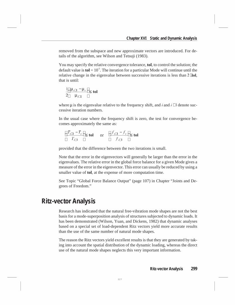
removed from the subspace and new approximate vectors are introduced. For de-tails of the algorithm, see Wilson and Tetsuji (1983).
You may specify the relative convergence tolerance,tol, to control the solution; thedefault value istol = 10-5. The iteration for a particular Mode will continue until therelative change in the eigenvalue between successive iterations is less than2 ⋅ tol,that is until:
1
2
1
1
µ µµi i
i
+
+
−
≤ tol
whereµ is the eigenvalue relative to the frequency shift, andi andi +1denote suc-cessive iteration numbers.
In the usual case where the frequency shift is zero, the test for convergence be-comes approximately the same as:
T T
T
f f
f
i i
i
i i
i
+
+
+
+
−
≤ −
≤1
1
1
1
tol tolor
provided that the difference between the two iterations is small.
Note that the error in the eigenvectors will generally be larger than the error in theeigenvalues. The relative error in the global force balance for a given Mode gives ameasure of the error in the eigenvector. This error can usually be reduced by using asmaller value oftol, at the expense of more computation time.
See Topic “Global Force Balance Output” (page 107) in Chapter “Joints and De-grees of Freedom.”
Ritz-vector AnalysisResearch has indicated that the natural free-vibration mode shapes are not the bestbasis for a mode-superposition analysis of structures subjected to dynamic loads. Ithas been demonstrated (Wilson, Yuan, and Dickens, 1982) that dynamic analysesbased on a special set of load-dependent Ritz vectors yield more accurate resultsthan the use of the same number of natural mode shapes.
The reason the Ritz vectors yield excellent results is that they are generated by tak-ing into account the spatial distribution of the dynamic loading, whereas the directuse of the natural mode shapes neglects this very important information.
Ritz-vector Analysis 299
Chapter XVI Static and Dynamic Analysis
317

The spatial distribution of the dynamic load vector serves as astarting load vectorto initiate the procedure. The first Ritz vector is the static displacement vector cor-responding to the starting load vector. The remaining vectors are generated from arecurrence relationship in which the mass matrix is multiplied by the previously ob-tained Ritz vector and used as the load vector for the next static solution. Each staticsolution is called ageneration cycle.
When the dynamic load is made up of several independent spatial distributions,each of these may serve as a starting load vector to generate a set of Ritz vectors.Each generation cycle creates as many Ritz vectors as there are starting load vec-tors. If a generated Ritz vector is redundant or does not excite any mass degrees offreedom, it is discarded and the corresponding starting load vector is removed fromall subsequent generation cycles.
Standard eigensolution techniques are used to orthogonalize the set of generatedRitz vectors, resulting in a final set of Ritz-vector Modes. Each Ritz-vector Modeconsists of a mode shape and frequency. The full set of Ritz-vector Modes can beused as a basis to represent the dynamic displacement of the structure.
Once the stiffness matrix is triangularized it is only necessary to statically solve forone load vector for each Ritz vector required. This results in an extremely efficientalgorithm. Also, the method automatically includes the advantages of the provennumerical techniques of static condensation, Guyan reduction, and static correctiondue to higher-mode truncation.
The algorithm is detailed in Wilson (1985).
When a sufficient number of Ritz-vector Modes have been found, some of themmay closely approximate natural mode shapes and frequencies. In general, how-ever, Ritz-vector Modes do not represent the intrinsic characteristics of the struc-ture in the same way the natural Modes do. The Ritz-vector modes are biased by thestarting load vectors.
You may specify the number of Modes to be found, the starting load vectors to beused, and the number of generation cycles to be performed for each starting loadvector. These parameters are described in the following subtopics.
Number of Modes
You may specify the total number of Modes,n, to be found. The total number ofModes actually found,n, is limited by:
• The number of Modes requested,n
300 Ritz-vector Analysis
SAP2000 Analysis Reference
318

• The number of mass degrees of freedom present in the model
• The number of natural free-vibration modes that are excited by the starting loadvectors (some additional natural modes may creep in due to numerical noise)
A mass degree of freedom is anyactivedegree of freedom that possesses transla-tional mass or rotational mass moment of inertia. The mass may have been assigneddirectly to the joint or may come from connected elements.
Only the Modes that are actually found will be available for any subsequentresponse-spectrum or time-history analysis processing.
See Topic “Degrees of Freedom” (page 83) in Chapter “Joints and Degrees of Free-dom.”
Starting Load Vectors
You may specify any number of starting load vectors. Each starting load vectormay be one of the following:
• An Acceleration Load in the global X, Y, or Z direction
• A Load Case
• A built-in nonlinear deformation load, as described below
For response-spectrum analysis, only the Acceleration Loads are needed. Fortime-history analysis, one starting load vector is needed for each Load Case or Ac-celeration Load that is used in any History.
If nonlinear time-history analysis is to be performed, an additional starting loadvector is needed foreachindependent nonlinear deformation. You may specify thatthe program use the built-in nonlinear deformation loads, or you may define yourown Load Cases for this purpose. See Topic “Nonlinear Deformation Loads” (page271) in Chapter “The Nllink Element” for more information.
If you define your own starting load vectors, do the following foreachnonlineardeformation:
• Explicitly define a Load Case that consists of a set of self-equilibrating forcesthat activates the desired nonlinear deformation
• Specify that Load Case as a starting load vector
The number of such Load Cases required is equal to the number of independentnonlinear deformations in the model.
Ritz-vector Analysis 301
Chapter XVI Static and Dynamic Analysis
319
If several Nllink elements act together, you may be able to use fewer starting loadvectors. For example, suppose the horizontal motion of several base isolators arecoupled with a diaphragm. Only three starting load vectors acting on the diaphragmare required: two perpendicular horizontal loads and one moment about the verticalaxis. Independent Load Cases may still be required to represent any vertical mo-tions or rotations about the horizontal axes for these isolators.
It is strongly recommendedthat mass (or mass moment of inertia) be present atevery degree of freedom that is loaded by a starting load vector. This is automaticfor Acceleration Loads, since the load is caused by mass. If a Load Case or nonlin-ear deformation load acts on a non-mass degree of freedom, the program issues awarning. Such starting load vectors may generate inaccurate Ritz vectors, or evenno Ritz vectors at all.
Generally, the more starting load vectors used, the more Ritz vectors must be re-quested to cover the same frequency range. Thus including unnecessary startingload vectors is not recommended.
In each generation cycle, Ritz vectors are found in the order in which the startingload vectors are specified. In the last generation cycle, only as many Ritz vectorswill be found as required to reach the total number of Modes,n. For this reason, themost important starting load vectors should be specified first, especially if thenumber of starting load vectors is not much smaller than the total number of Modes.
If no starting load vectors are explicitly specified, the three Acceleration Loads areused by default. This is adequate for response-spectrum analysis and linear seismictime-history analysis with no other loads applied.
For more information:
• See Topic “Nonlinear Time-History Analysis” (page 328) in this chapter.
• See Chapter “Load Cases” (page 279).
Number of Generation Cycles
You may specify the maximum number of generation cycles,ncyc, to be performedfor each starting load vector. This enables you to obtain more Ritz vectors for somestarting load vectors than others. By default, the number of generation cycles per-formed for each starting load vector is unlimited, i.e., until the total number,n, ofrequested Ritz vectors have been found.
As an example, suppose that two linear time-history analyses are to be performed:
302 Ritz-vector Analysis
SAP2000 Analysis Reference
320

(1) Gravity load is applied quasi-statically to the structure using Load Cases DLand LL
(2) Seismic load is applied in all three global directions starting from the condi-tions at the end of the first History
The starting load vectors required are the three Acceleration Loads and Load CasesDL and LL. The first generation cycle creates the static solution for each startingload vector. This is all that is required for Load Cases DL and LL in the first His-tory, hence for these starting load vectorsncyc= 1 should be specified. AdditionalModes may be required to represent the dynamic response to the seismic loading,hence an unlimited number of cycles should be specified for these starting load vec-tors. If 12 Modes are requested (n = 12), there will be one each for DL and LL, threeeach for two of the Acceleration Loads, and four for the Acceleration Load that wasspecified first as a starting load vector.
Starting load vectors corresponding to nonlinear deformation loads may often needonly a limited number of generation cycles. Many of these loads affect only a smalllocal region and excite only high-frequency natural modes that may respond quasi-statically to typical seismic excitation. If this is the case, you may be able to specifyncyc= 1 or 2 for these starting load vectors. More cycles may be required if you areparticularly interested in the dynamic behavior in the local region.
You must use your own engineering judgment to determine the number of Ritz vec-tors to be generated for each starting load vector. No simple rule can apply to allcases.
Modal Analysis OutputVarious properties of the Vibration Modes are printed in the output file. This infor-mation is the same regardless of whether you use eigenvector or Ritz-vector analy-sis, and is described in the following subtopics.
Typical modal-analysis output is shown in Figure 84 (page 305).
Periods and Frequencies
The following time-properties are printed for each Mode:
• Period,T, in units of time
• Cyclic frequency,f, in units of cycles per time; this is the inverse ofT
Modal Analysis Output 303
Chapter XVI Static and Dynamic Analysis
321

• Circular frequency,ω, in units of radians per time;ω = 2 π f
• Eigenvalue,ω2, in units of radians-per-time squared
These can be found in the output file under the heading:
MODAL PERIODS AND FREQUENCIES
Participation Factors
The modal participation factors are the dot products of the three Acceleration Loadswith the modes shapes. The participation factors for Moden corresponding to Ac-celeration Loads in the global X, Y, and Z directions are given by:
f xn n x= ϕ T
m
f yn n y= ϕ T
m
f zn n z= ϕ T
m
whereϕ n is the mode shape andmx, my, and,mz are the unit Acceleration Loads.These factors are the generalized loads acting on the Mode due to each of the Accel-eration Loads. They are referred to the global coordinate system and can be foundin the output file under the heading:
MODAL PARTICIPATION FACTORS
These values are called “factors” because they are related to the mode shape and toa unit acceleration. The modes shapes are each normalized, or scaled, with respectto the mass matrix such that:
ϕ ϕn nT
M =1
The actual magnitudes and signs of the participation factors are not important.What is important is the relative values of the three factors for a given Mode.
Participating Mass Ratios
The participating mass ratio for a Mode provides a measure of how important theMode is for computing the response to the Acceleration Loads in each of the threeglobal directions. Thus it is useful for determining the accuracy of response-spectrum analyses and seismic time-history analyses. The participating mass ratio
304 Modal Analysis Output
SAP2000 Analysis Reference
322

Modal Analysis Output 305
Chapter XVI Static and Dynamic Analysis
M O D A L P E R I O D S A N D F R E Q U E N C I E S
MODE PERIOD FREQUENCY FREQUENCY EIGENVALUE(TIME) (CYC/TIME) (RAD/TIME) (RAD/TIME)**2
1 2.425536 0.412280 2.590431 6.7103342 2.407723 0.415330 2.609596 6.8099913 2.134032 0.468596 2.944279 8.6687764 0.233621 4.280440 26.894795 723.3299995 0.229738 4.352780 27.349324 747.9855156 0.168388 5.938672 37.313777 1392.3187 0.131499 7.604615 47.781207 2283.0448 0.115861 8.631016 54.230275 2940.923
M O D A L P A R T I C I P A T I O N F A C T O R S
FOR UNIT ACCELERATION LOADS IN GLOBAL COORDINATES
MODE PERIOD UX UY UZ1 2.425536 1.391631 1.732188 -7.71E-052 2.407723 -1.781824 1.426170 -0.0002683 2.134032 -0.312429 -0.418085 0.0001144 0.233621 0.027199 -0.000259 -0.0179825 0.229738 8.72E-05 0.025523 0.0568656 0.168388 -6.46E-05 -0.000624 2.1729567 0.131499 -0.000283 0.002020 0.0720188 0.115861 0.000830 0.000853 0.373158
M O D A L P A R T I C I P A T I N G M A S S R A T I O S
MODE PERIOD INDIVIDUAL MODE (PERCENT) CUMULATIVE SUM (PERCENT)UX UY UZ UX UY UZ
1 2.425536 37.1724 57.5919 0.0000 37.1724 57.5919 0.00002 2.407723 60.9398 39.0404 0.0000 98.1122 96.6323 0.00003 2.134032 1.8736 3.3551 0.0000 99.9858 99.9874 0.00004 0.233621 0.0142 0.0000 0.0062 100.0000 99.9874 0.00625 0.229738 0.0000 0.0125 0.0621 100.0000 99.9999 0.06836 0.168388 0.0000 0.0000 90.6304 100.0000 99.9999 90.69867 0.131499 0.0000 0.0001 0.0996 100.0000 100.0000 90.79828 0.115861 0.0000 0.0000 2.6727 100.0000 100.0000 93.4709
M O D A L L O A D P A R T I C I P A T I O N R A T I O S
LOAD, ACC, OR NLLINK/DEF STATIC DYNAMIC(TYPE) (NAME) (PERCENT) (PERCENT)
LOAD GRAVITY 100.0000 -> 93.4709<- EXCLUDES LOAD ON NON-MASS DOFACC UX 100.0000 100.0000ACC UY 100.0000 100.0000ACC UZ 99.0042 93.4709
NLLINK/DEF 1/U1 100.0000 31.6238NLLINK/DEF 1/U2 100.0000 67.2915NLLINK/DEF 1/U3 100.0000 63.9055NLLINK/DEF 2/U1 100.0000 37.9576NLLINK/DEF 2/U2 100.0000 67.2915NLLINK/DEF 2/U3 100.0000 89.9700NLLINK/DEF 3/U1 5.3432 0.8109NLLINK/DEF 3/U2 100.0000 67.2915NLLINK/DEF 3/U3 100.0000 57.5064
Figure 84Modal Analysis Output in the Output File
323

providesno informationabout the accuracy of time-history analyses subjected toother loads.
The participating mass ratios for Moden corresponding to Acceleration Loads inthe global X, Y, and Z directions are given by:
rf
Mxn
xn
x
= ( )2
rf
Myn
yn
y
=( )
2
rf
Mzn
zn
z
= ( )2
wherefxn, fyn, andfzn are the participation factors defined in the previous subtopic;andMx, My, andMz are the total unrestrained masses acting in the X, Y, and Z direc-tions. The participating mass ratios are expressed as percentages and printed in theoutput file under the heading:
MODAL PARTICIPATING MASS RATIOS
The cumulative sums of the participating mass ratios for all Modes up to Modenare printed with the individual values for Moden. This provides a simple measureof how many Modes are required to achieve a given level of accuracy for ground-acceleration loading.
If all eigen Modes of the structure are present, the participating mass ratio for eachof the three Acceleration Loads should generally be 100%. However, this may notbe the case in the presence of Asolid elements or certain types of Constraints wheresymmetry conditions prevent some of the mass from responding to translational ac-celerations.
Static and Dynamic Load Participation Ratios
The static and dynamic load participation ratios provide a measure of how adequatethe calculated modes are for representing the response to time-history analyses.These two measures are printed in the output file for each of the following spatialload vectors:
• The three unit Acceleration Loads
• All static Load Cases
306 Modal Analysis Output
SAP2000 Analysis Reference
324

• All nonlinear deformation loads
The first two represent spatial loads that you can explicitly specify in a time-historyanalysis, whereas the last represents loads that can act implicitly in anonlineartime-history analysis.
The load participation ratios, expressed as percentages, are printed in the output fileunder the heading:
MODAL LOAD PARTICIPATION RATIOS
For more information:
• See Topic “Nonlinear Deformation Loads” (page 271) in Chapter “The NllinkElement.”
• See Chapter “Load Cases” (page 279).
• See Topic “Acceleration Loads” (page 295) in this chapter.
• See Topic “Time-History Analysis” (page 319) in this chapter.
• See Topic “Nonlinear Time-History Analysis” (page 328) in this chapter.
Static Load Participation Ratio
The static load participation ratio measures how well the calculated modes can rep-resent the response to a given static load. This measure was first presented by Wil-son (1997). For a given spatial load vectorp, the participation factor for Moden isgiven by
f n n= ϕ T
p
whereϕ n is the mode shape (vector) of Moden. This factor is the generalized load
acting on the Mode due to loadp. Note thatf n is just the usual participation factorwhenp is one of the unit acceleration loads.
The static participation ratio for this mode is given by
r
f
nS
n
n=
ω
2
u pT
whereu is the static solution given byKu p= . This ratio gives the fraction of the to-tal strain energy in the exact static solution that is contained in Moden. Note thatthe denominator can also be represented asu Ku
T .
Modal Analysis Output 307
Chapter XVI Static and Dynamic Analysis
325

Finally, the cumulative sum of the static participation ratios for all the calculatedmodes is printed in the output file:
R rS
nS
n
N
n
nn
N
= =
=
=∑∑
1
2
1
ϕω
T
T
p
u p
whereN is the number of modes found. This value gives the fraction of the totalstrain energy in the exact static solution that is captured by theN modes.
When solving for static solutions using quasi-static time-history analysis, the valueof R
S should be close to 100% for any applied static Loads, and also for all nonlin-ear deformation loads if the analysis is nonlinear.
Note that when Ritz-vectors are used, the value ofRS will always be 100% for all
starting load vectors. This may not be true when eigenvectors are used. In fact, evenusing all possible eigenvectors will not give 100% static participation if loadp actson any massless degrees-of-freedom.
Dynamic Load Participation Ratio
The dynamic load participation ratio measures how well the calculated modes canrepresent the response to a given dynamic load. This measure was developed forSAP2000, and it is an extension of the concept of participating mass ratios. It is as-sumed that the load acts only on degrees of freedom with mass. Any portion of loadvectorp that acts on massless degrees of freedom cannot be represented by thismeasure and is ignored in the following discussion.
For a given spatial load vectorp, the participation factor for Moden is given by
f n n= ϕ T
p
whereϕ n is the mode shape for Moden. Note thatf n is just the usual participation
factor whenp is one of the unit acceleration loads.
The dynamic participation ratio for this mode is given by
( )r
fnD n=
2
a pT
308 Modal Analysis Output
SAP2000 Analysis Reference
326

wherea is the acceleration given byMa p= . The accelerationa is easy to calculatesinceM is diagonal. The values ofa andp are taken to be zero at all massless de-grees of freedom. Note that the denominator can also be represented asa Ma
T .
Finally, the cumulative sum of the dynamic participation ratios for all the calcu-lated modes is printed in the output file:
( )R r
DnD
n
N n
n
N
= ==
=∑∑
1
2
1
ϕ T
T
p
a p
whereN is the number of modes found. Whenp is one of the unit acceleration loads,rD is the usual mass participation ratio, andR
D is the usual cumulative mass par-ticipation ratio.
WhenRD is 100%, the calculated modes should be capable of exactly representingthe solution to any time-varying application of spatial loadp. If R
D is less than100%, the accuracy of the solution will depend upon the frequency content of thetime-function multiplying loadp. Normally it is the high frequency response that isnot captured whenRD is less than 100%.
The dynamic load participation ratio only measures how the modes capture the spa-tial characterisitcs ofp, not its temporal characteristics. For this reason,R
D servesonly as a qualitative guide as to whether enough modes have been computed. Youmust still examine the response to each different dynamic loading with varyingnumber of modes to see if enough modes have been used.
FunctionsA Function is a series of digitized abscissa-ordinate pairs that may represent:
• Pseudo-spectral acceleration vs. period for response-spectrum analysis, or
• Load vs. time for time-history analysis
You may define any number of Functions, assigning each one a unique label. Youmay scale the abscissa and/or ordinate values whenever the Function is used.
The abscissa of a Function is always time or period (which has time units). Theabscissa-ordinate pairs must be specified in order of increasing time value.
Functions 309
Chapter XVI Static and Dynamic Analysis
327

If the increment between time values (abscissas) is constant and the Function startsat time zero, you need only specify the time increment,dt, and the successive func-tion values (ordinates) starting at time zero. The function values are specified as:
f0, f1, f2, ...,fn
corresponding to times:
0, dt, 2dt, ...,n dt
wheren + 1 is the number of values given.
If the time increment is not constant or the Function does not start at time zero, youmust specify the pairs of time and function value as:
t0, f0, t1, f1, t2, f2, ...,tn, fn
where n + 1 is the number of pairs of values given.
Response-Spectrum AnalysisThe dynamic equilibrium equations associated with the response of a structure toground motion are given by:
K u C u M u m m m( ) &( ) &&( ) && ( ) && ( ) &&t t t u t u t ux gx y gy z gz+ + = + + ( )t
whereK is the stiffness matrix;C is the proportional damping matrix;M is the di-agonal mass matrix;u, &u, and&&u are the relative displacements, velocities, and accel-erations with respect to the ground;mx, my, andmz are the unit Acceleration Loads;and&&ugx, &&ugy, and&&ugz are the components of uniform ground acceleration.
Response-spectrum analysis seeks the likely maximum response to these equationsrather than the full time history. The earthquake ground acceleration in each direc-tion is given as a digitized response-spectrum curve of pseudo-spectral accelerationresponse versus period of the structure.
Even though accelerations may be specified in three directions, only a single, posi-tive result is produced for each response quantity. The response quantities includedisplacements, forces, and stresses. Each computed result represents a statisticalmeasure of the likely maximum magnitude for that response quantity. The actualresponse can be expected to vary within a range from this positive value to its nega-tive.
310 Response-Spectrum Analysis
SAP2000 Analysis Reference
328

No correspondence between two different response quantities is available. No in-formation is available as to when this extreme value occurs during the seismic load-ing, or as to what the values of other response quantities are at that time.
Response-spectrum analysis is performed using mode superposition (Wilson andButton, 1982). Modes may have been computed using eigenvector analysis orRitz-vector analysis. Ritz vectors are recommended since they give more accurateresults for the same number of Modes.
Any number of response-spectrum analyses can be performed in a single executionof the program. Each analysis case is called aSpec, to which you assign a unique la-bel. Each Spec can differ in the acceleration spectra applied and in the way that re-sults are combined. Results from each Spec can be output directly or used in Com-bos.
The following subtopics describe in more detail the parameters that you use to de-fine each Spec.
Local Coordinate System
Each Spec has its ownresponse-spectrum local coordinate systemused to definethe directions of ground acceleration loading. The axes of this local system are de-noted 1, 2, and 3. By default these correspond to the global X, Y, and Z directions,respectively.
You may change the orientation of the local coordinate system by specifying:
• A fixed coordinate systemcsys(the default is zero, indicating the global coor-dinate system)
• A coordinate angle,ang (the default is zero)
The local 3 axis is always the same as the Z axis of coordinate systemcsys. The lo-cal 1 and 2 axes coincide with the X and Y axes ofcsysif angleang is zero. Other-wise,ang is the angle from the X axis to the local 1 axis, measured counterclock-wise when the +Z axis is pointing toward you. This is illustrated in Figure 85 (page312).
Response-Spectrum Curve
The response-spectrum curve for a given direction is defined by digitized points ofpseudo-spectral acceleration response versus period of the structure. The shape of
Response-Spectrum Analysis 311
Chapter XVI Static and Dynamic Analysis
329

the curve is given by specifying the name of a Function. All values for the abscissaand ordinate of this Function must be zero or positive.
If no Function is specified, a constant function of unit acceleration value for all pe-riods is assumed.
You may specify a scale factorsf to multiply the ordinate (pseudo spectral accelera-tion response) of the function. This is often needed to convert values given in termsof the acceleration due to gravity to units consistent with the rest of the model. SeeFigure 86 (page 313).
The response-spectrum curve chosen should reflect the damping that is present inthe structure being modeled. Note that the damping is inherent in the response-spectrum curve itself. It is not affected by the damping ratio,damp, used for theCQC or GMC method of modal combination, although normally these two damp-ing values should be the same.
If the response-spectrum curve is not defined over a period range large enough tocover the Vibration Modes of the structure, the curve is extended to larger andsmaller periods using a constant acceleration equal to the value at the nearest de-fined period.
See Topic “Functions” (page 309) in this chapter for more information.
312 Response-Spectrum Analysis
SAP2000 Analysis Reference
Figure 85Definition of Response Spectrum Local Coordinate System
330

Modal Combination
For a given direction of acceleration, the maximum displacements, forces, andstresses are computed throughout the structure for each of the Vibration Modes.These modal values for a given response quantity are combined to produce a single,positive result for the given direction of acceleration using one of the followingmethods. Use the parametermodc to specify which method to use.
CQC Method
Specifymodc = CQC to combine the modal results by the Complete QuadraticCombination technique described by Wilson, Der Kiureghian, and Bayo (1981).This is the default method of modal combination.
The CQC method takes into account the statistical coupling between closely-spaced Modes caused by modal damping. Increasing the modal damping increasesthe coupling between closely-spaced modes. If the damping is zero for all Modes,this method degenerates to the SRSS method.
Modal damping comes from two sources:
Response-Spectrum Analysis 313
Chapter XVI Static and Dynamic Analysis
Figure 86Digitized Response-Spectrum Curve
331

• You may specify a CQC damping ratio,damp, measured as a fraction of criti-cal damping:0 1≤ <damp . This damping equally affects all Modes, and shouldreflect the damping that is present in the structure being modeled. Note that thevalue ofdamp does not affect the response-spectrum curve, which is devel-oped independently for an assumed value of structural damping. Normallythese two damping values should be the same.
• You may specify non-zero effective-damping coefficients for any Nllink ele-ments in the model. These effective damping values are converted to modaldamping ratios by assuming proportional damping, i.e., by ignoring any modalcross-coupling terms. These effective modal-damping values will generally bedifferent for each Mode, depending upon how much deformation each Modecauses in the Nllink elements. Only effective damping, not actual damping, inthe Nllink elements affects the CQC results.
The total damping ratio for each Mode is the sum of these two sources. The pro-gram will automatically make sure that the total is less than one.
GMC Method
Specifymodc= GMC to combine the modal results by the General Modal Combi-nation technique. This method is the same as the complete modal combination pro-cedure described by Equation 3.31 in Gupta (1990). The GMC method takes intoaccount the statistical coupling between closely-spaced Modes similarly to theCQC method, but also includes the correlation between modes with rigid-responsecontent.
Increasing the modal damping increases the coupling between closely-spacedmodes. As with the CQC method, modal damping comes from the two sources:
• You may specify a GMC damping ratio,damp, such that0 1≤ <damp . This
damping equally affects all Modes.
• Additional modal damping is computed from the effective-damping coeffi-cients for any Nllink elements in the model
See the CQC method above for more information on modal damping.
In addition, the GMC method requires you to specify two frequencies,f1 andf2,which define the rigid-response content of the ground motion. These must satisfy0< <f1 f2. The rigid-response parts of all modes are assumed to be perfectly corre-lated.
314 Response-Spectrum Analysis
SAP2000 Analysis Reference
332

The GMC method assumes no rigid response below frequencyf1, full rigid re-sponse above frequencyf2, and an interpolated amount of rigid response for fre-quencies betweenf1 andf2.
Frequenciesf1 andf2 are properties of the seismic input, not of the structure. Guptadefinesf1 as:
f1 = S
S
A
V
max
max2π
whereS Amaxis the maximum spectral acceleration andSVmax
is the maximumspectral velocity for the ground motion considered. The default value forf1 is unity.
Gupta definesf2 as:
f2 f1= +1
3
2
3f r
where f r is the rigid frequency of the seismic input, i.e., that frequency abovewhich the spectral acceleration is essentially constant and equal to the value at zeroperiod (infinite frequency). Others have definedf2 as:
f2 = f r
The default value forf2 is zero, indicating infinite frequency. For the default valueof f2, the GMC method gives results similar to the CQC method.
SRSS Method
Specifymodc= SRSS to combine the modal results by taking the square root of thesum of their squares. This method does not take into account any coupling ofModes as do the CQC and GMC methods.
Absolute Sum Method
Specifymodc= ABS to combine the modal results by taking the sum of their abso-lute values. This method is usually over-conservative.
Directional Combination
For each displacement, force, or stress quantity in the structure, modal combinationproduces a single, positive result for each direction of acceleration. These direc-tional values for a given response quantity are combined to produce a single, posi-
Response-Spectrum Analysis 315
Chapter XVI Static and Dynamic Analysis
333
tive result. Use the directional combination scale factor,dirf , to specify whichmethod to use.
SRSS Method
Specifydirf = 0 to combine the directional results by taking the square root of thesum of their squares. This method is invariant with respect to coordinate system,i.e., the results do not depend upon your choice of coordinate system when thegiven response-spectrum curves are the same. This is the recommended method fordirectional combination, and is the default.
Absolute Sum Method
Specifydirf = 1 to combine the directional results by taking the sum of their abso-lute values. This method is usually over-conservative.
Scaled Absolute Sum Method
Specify 0 <dirf < 1 to combine the directional results by the scaled absolute summethod. Here, the directional results are combined by taking the maximum, over alldirections, of the sum of the absolute values of the response in one direction plusdirf times the response in the other directions.
For example, ifdirf = 0.3, the spectral response,R, for a given displacement, force,or stress would be:
R R R R= max ( , , )1 2 3
where:
R R R R1 1 2 3
03= + +. ( )
R R R R2 2 1 3
03= + +. ( )
R R R R3 3 1 2
03= + +. ( )
andR1, R
2, andR
3are the modal-combination values for each direction.
The results obtained by this method will vary depending upon the coordinate sys-tem you choose. Results obtained usingdirf = 0.3 are comparable to the SRSSmethod (for equal input spectra in each direction), but may be as much as 8% un-conservative or 4% over-conservative, depending upon the coordinate system.Larger values ofdirf tend to produce more conservative results.
316 Response-Spectrum Analysis
SAP2000 Analysis Reference
334

Response-Spectrum Analysis OutputCertain information is printed in the output file for each response-spectrum analy-sis. This information is described in the following subtopics.
Typical response-spectrum analysis output is shown in Figure 87 (page 318).
Damping and Accelerations
The modal damping and the ground accelerations acting in each direction areprinted for every Mode under the heading:
RESPONSE SPECTRUM ACCELERATIONS
The damping value printed for each Mode is the sum of the specified CQC or GMCdamping ratio,damp, plus the modal damping contributed by effective damping inthe Nllink elements, if any.
The accelerations printed for each Mode are the actual values as interpolated at themodal period from the response-spectrum curves after scaling by the specified val-ues ofsf and tf . The accelerations are always referred to the local axes of theresponse-spectrum analysis. They are identified in the output as U1, U2, and U3.
Modal Amplitudes
The response-spectrum modal amplitudes give the multipliers of the mode shapesthat contribute to the displaced shape of the structure for each direction of Accelera-tion. For a given Mode and a given direction of acceleration, this is the product ofthe modal participation factor and the response-spectrum acceleration, divided bythe eigenvalue,ω2, of the Mode. These values are printed in the output file under theheading:
RESPONSE SPECTRUM MODAL AMPLITUDES
The acceleration directions are always referred to the local axes of the response-spectrum analysis. They are identified in the output as U1, U2, and U3.
For more information:
• See the previous Subtopic “Damping and Acceleration” for the definition of theresponse-spectrum accelerations.
• See Topic “Modal Analysis Output” (page 303) in this chapter for the defini-tion of the modal participation factors and the eigenvalues.
Response-Spectrum Analysis Output 317
Chapter XVI Static and Dynamic Analysis
335

318 Response-Spectrum Analysis Output
SAP2000 Analysis Reference
R E S P O N S E S P E C T R U M A C C E L E R A T I O N S
IN RESPONSE-SPECTRUM LOCAL COORDINATES
SPEC 1 ------------------
MODE PERIOD DAMP-RATIO U1 U2 U31 0.414601 0.050000 29.443875 29.443875 .0000002 0.375298 0.050000 28.919579 28.919579 .0000003 0.243572 0.050000 26.554969 26.554969 .000000
R E S P O N S E S P E C T R U M M O D A L A M P L I T U D E S
IN RESPONSE-SPECTRUM LOCAL COORDINATES
SPEC 1 ------------------
MODE PERIOD U1 U2 U31 0.414601 -0.168018 -0.286686 .0000002 0.375298 -0.231232 0.135573 .0000003 0.243572 0.010526 -0.006012 .000000
R E S P O N S E S P E C T R U M M O D A L C O R R E L A T I O N S
PARTIAL MATRIX SHOWING CORRELATION FACTORS BETWEEN NEARBY MODES
SPEC 1 ------------------
MODE I PERIOD I I+1 I+2 I+3 I+4 I+5 I+6 I+7 I+8 I+91 0.414601 1.000 0.501 0.0322 0.375298 1.000 0.0493 0.243572 1.000
R E S P O N S E S P E C T R U M B A S E R E A C T I O N S
IN RESPONSE-SPECTRUM LOCAL COORDINATES
SPEC 1 ------------------
FOR EACH MODE, DUE TO SPECTRAL ACCELERATION IN DIRECTION U1:
MODE F1 F2 F3 M1 M2 M31 50.572403 86.290877 .000000 -1830.315 1072.735 2492.2632 145.250875 -85.161739 .000000 1793.046 3058.354 -2132.8183 1.847642 -1.055259 .000000 20.956121 36.678180 -26.348178
FOR EACH MODE, DUE TO SPECTRAL ACCELERATION IN DIRECTION U2:
MODE F1 F2 F3 M1 M2 M31 86.290877 147.236736 .000000 -3123.037 1830.390 4252.5082 -85.161739 49.931002 .000000 -1051.277 -1793.137 1250.4883 -1.055259 0.602698 .000000 -11.968838 -20.948303 15.048447
COMBINED FOR ALL MODES AND ALL DIRECTIONS OF SPECTRAL ACCELERATION:
F1 F2 F3 M1 M2 M3SPEC 195.935537 197.196505 .000000 4174.970 4133.414 5515.265
Figure 87Response-Spectrum Analysis Output in the Output File
336

Modal Correlation Factors
When the type of modal combination is either CQC or GMC, a partial modal corre-lation matrix is printed out. This matrix shows the coupling assumed betweenclosely-spaced modes. The correlation factors are always between zero and one.The correlation factors coupling each mode with the next nine higher modes areprinted in the output file under the heading:
RESPONSE SPECTRUM MODAL CORRELATIONS
The correlation matrix is symmetric.
Base Reactions
The base reactions are the total forces and moments about the global origin requiredof the supports (Restraints and Springs) to resist the inertia forces due to response-spectrum loading. These are printed in the output file under the heading:
RESPONSE SPECTRUM BASE REACTIONS
These are printed separately for each individual Mode and each direction of loadingwithout any combination. The total response-spectrum reactions are then printedafter performing modal combination and directional combination.
The reaction forces and moments are always referred to the local axes of theresponse-spectrum analysis. They are identified in the output as F1, F2, F3, M1,M2, and M3.
Time-History AnalysisTime-history analysis is used to determine the dynamic response of a structure toarbitrary loading. The dynamic equilibrium equations to be solved are given by:
K u C u M u r( ) &( ) &&( ) ( )t t t t+ + =
whereK is the stiffness matrix;C is the proportional damping matrix;M is the di-agonal mass matrix;u, &u, and&&u are the relative displacements, velocities, and accel-erations with respect to the ground; andr is the applied load.
Any number of time-history analyses can be performed in a single execution of theprogram. Each analysis case is called aHistory , to which you assign a unique label.Each History can differ in the load applied and in the type of analysis to be per-formed.
Time-History Analysis 319
Chapter XVI Static and Dynamic Analysis
337

Three types of time-history analysis are available:
• Linear transient: The structure starts with zero initial conditions or with theconditions at the end of a previous linear transient History that you specify. Allelements are assumed to behave linearly for the duration of the analysis.
• Periodic: The initial conditions are adjusted to be equal to the those at the end ofthe period of analysis. All elements are assumed to behave linearly for the dura-tion of the analysis.
• Nonlinear transient: The structure starts with zero initial conditions or with theconditions at the end of a previous nonlinear transient History that you specify.The Nllink elements may exhibit nonlinear behavior during the analysis. Allother elements behave linearly.
P-Delta analysis, if requested, is performed before any time-history analyses.
This topic describes features that are common to all three types of analysis. Addi-tional features applying only to nonlinear transient analysis are described in theTopic “Nonlinear Time-History Analysis” (page 328) in this chapter.
Loading
The load,r(t), applied in a given History may be an arbitrary function of space andtime. It can be written as a finite sum of spatial load vectors,pi , multiplied by timefunctions,f ti ( ), as:
(Eqn. 1)r p( ) ( )t f ti i
i
= ∑The program uses Load Cases and/or Acceleration Loads to represent the spatialload vectors. The time functions can be arbitrary functions of time or periodic func-tions such as those produced by wind or sea wave loading.
If Acceleration Loads are used, the displacements, velocities, and accelerations areall measured relative to the ground. The time functions associated with the Accel-eration Loadsmx, my, andmz are the corresponding components of uniform groundacceleration,&&ugx, &&ugy, and&&ugz .
Defining the Spatial Load Vectors
To define the spatial load vector,pi, for a single term of the loading sum of Equation1, you may specify either:
• The label of a Load Case using the parameterload, or
320 Time-History Analysis
SAP2000 Analysis Reference
338

• An Acceleration Load using the parameterscsys, ang, andacc, where:
– csysis a fixed coordinate system (the default is zero, indicating the globalcoordinate system)
– ang is a coordinate angle (the default is zero)
– accis the Acceleration Load (U1, U2, or U3) in the acceleration local coor-dinate system as defined below
Each Acceleration Load in the loading sum may have its own acceleration local co-ordinate system with local axes denoted 1, 2, and 3. The local 3 axis is always thesame as the Z axis of coordinate systemcsys. The local 1 and 2 axes coincide withthe X and Y axes ofcsysif angleang is zero. Otherwise,ang is the angle from the Xaxis to the local 1 axis, measured counterclockwise when the +Z axis is pointing to-ward you. This is illustrated in Figure 88 (page 321).
The response-spectrum local axes are always referred to as 1, 2, and 3. The globalAcceleration Loadsmx, my, andmz are transformed to the local coordinate systemfor loading.
It is generally recommended, but not required, that the same coordinate system beused for all Acceleration Loads applied in a given History.
Load Cases and Acceleration Loads may be mixed in the loading sum.
For more information:
Time-History Analysis 321
Chapter XVI Static and Dynamic Analysis
Figure 88Definition of History Acceleration Local Coordinate System
339

• See Chapter “Load Cases” (page 279).
• See Topic “Acceleration Loads” (page 295) in this chapter.
Defining the Time Functions
To define the time function,fi(t), for a single term of the loading sum of Equation 1,you may specify:
• The label of a Function, using the parameterfunc, that defines the shape of thetime variation (the default is zero, indicating the built-in ramp function definedbelow)
• A scale factor,sf, that multiplies the ordinate values of the Function (the defaultis unity)
• A time-scale factor,tf , that multiplies the time (abscissa) values of the Function(the default is unity)
• An arrival time,at, when the Function begins to act on the structure (the defaultis zero)
The time function,fi(t), is related to the specified Function,func(t), by:
fi(t) = sf · func(t)
The analysis time,t, is related to the time scale,t, of the specified Function by:
t = at + tf · t
If the arrival time is positive, the application of Functionfunc is delayed until afterthe start of the analysis. If the arrival time is negative, that portion of Functionfuncoccurring beforet = – at / tf is ignored.
For a Functionfunc defined from initial timet0 to final time tn, the value of theFunction for all timet < t0 is taken as zero, and the value of the Function for all timet > tn is held constant atfn, the value attn.
If no Function is specified, orfunc = 0, the built-in ramp function is used. Thisfunction increases linearly from zero att =0 to unity att =1and for all time thereaf-ter. When combined with the scaling parameters, this defines a function that in-creases linearly from zero att = at to a value ofsfatt = at + tf and for all time there-after, as illustrated in Figure 88 (page 323). This function is most commonly used togradually apply static loads, but can also be used to build up triangular pulses andmore complicated functions.
322 Time-History Analysis
SAP2000 Analysis Reference
340

See Topic “Functions” (page 309) in this chapter for more information.
Mode Superposition
The standard mode-superposition method of response analysis is used by the pro-gram to solve the dynamic equilibrium equations of motion for the complete struc-ture. The Modes used can be the undamped free-vibration Modes (eigenvectors) orthe load-dependent Ritz-vector Modes.
If all of the spatial load vectors,pi , are used as starting load vectors for Ritz-vectoranalysis, then the Ritz vectors will always produce more accurate results than if thesame number of eigenvectors is used. Since the Ritz-vector algorithm is faster thanthe eigenvector algorithm, the former is recommended for time-history analyses.
It is up to you to determine if the Modes calculated by the program are adequate torepresent the time-history response to the applied load. You should check:
• That enough Modes have been computed
• That the Modes cover an adequate frequency range
• That the participating mass ratios are adequate if Acceleration Loads are ap-plied
Time-History Analysis 323
Chapter XVI Static and Dynamic Analysis
Figure 89Built-in Ramp Function before and after Scaling
341

• That the modes shapes adequately represent all desired deformations
• That the global force balance for each Mode is acceptable
Special considerations must be made for the Modes used when performing nonlin-ear analysis. See Topic “Nonlinear Time-History Analysis” (page 328) in this chap-ter for more information.
For more information:
• See Topic “Eigenvector Analysis” (page 296) in this chapter.
• See Topic “Ritz-vector Analysis” (page 299) in this chapter.
• See Subtopic “Participating Mass Ratios” (page 304) in this chapter
• See Topic “Global Force Balance Output” (page 107) in Chapter “Joints andDegrees of Freedom.”
Modal Damping
The damping in the structure is modeled using modal damping, also known as pro-portional or classical damping. The damping in each Mode may be specified usingthe parameterdamp, which is measured as a fraction of critical damping. Thedamping value for each Mode must satisfy:
0 1≤ <damp
For a nonlinear transient analysis, this is the only source of modal damping. SeeTopic “Nonlinear Time-History Analysis” (page 328) for important considerationsabout using modal damping with nonlinear transient analysis.
For linear transient and periodic analyses, additional modal damping may comefrom any non-zero effective-damping coefficients that may be specified for Nllinkelements in the model. These effective damping values are converted to modaldamping ratios assuming proportional damping, i.e., by ignoring any modal cross-coupling terms. These effective modal-damping values will generally be differentfor each Mode, depending upon how much deformation each Mode causes in theNllink elements.
Only effective damping, not the actual damping in the Nllink elements, affects thelinear time-history results. The total damping ratio for each Mode is the sum ofthese two sources. The program automatically makes sure that the total is less thanone.
324 Time-History Analysis
SAP2000 Analysis Reference
342

Time Steps
Time-history analysis is performed at discrete time steps. You may specify thenumber of time steps with parameternstepand the size of the time steps with pa-rameterdt.
The time span over which the analysis is carried out is given bynstep·dt. For peri-odic analysis, the period of the cyclic loading function is assumed to be equal to thistime span.
Responses are calculated at the end of eachdt time increment, resulting innstep+1values for each output response quantity.
For linear transient and periodic analysis, closed-form integration of the modalequations is used to compute the response, assuming linear variation of the timefunctions,f ti ( ), between the input data time points. Therefore, numerical instabil-ity problems are never encountered, and the time increment may be any samplingvalue that is deemed fine enough to capture the maximum response values. One-tenth of the time period of the highest mode is usually recommended; however, alarger value may give an equally accurate sampling if the contribution of the highermodes is small.
For nonlinear transient analysis, closed-form integration is again used to computethe response, with the forces from the nonlinear Nllink elements applied to theright-hand side of the dynamic modal equilibrium equations. Since these forces de-pend upon the dynamic response, the solution is iterated at each time step until thenonlinear forces converge. The accuracy of the results may depend upon the size ofthe time step, improving with decreasingdt. See Topic “Nonlinear Time-HistoryAnalysis” (page 328) in this chapter for more information.
Initial Conditions
The initial conditions describe the state of the structure at the beginning of a His-tory. These include:
• Displacements and velocities
• Internal forces and stresses
• Internal state variables for the Nllink elements, if any
• Energy values for the structure
The accelerations are not considered initial conditions, but are computed from theequilibrium equation.
Time-History Analysis 325
Chapter XVI Static and Dynamic Analysis
343

For each linear and nonlinear transient analysis to be performed, you may use theparameterprev to specify the initial conditions to be used. It is not applicable to pe-riodic analyses.
If prev = 0 (the default), zero initial conditions are assumed for all displacements,velocities, energies, and the internal state variables. The initial acceleration of thestructure is computed by equilibrium using the applied loads and/or ground accel-erations at timet = 0.
Otherwiseprev must be the label of a previous History of the same type (linear ornonlinear transient) as the current History. The initial conditions of the current His-tory are taken to be the conditions that existed at the end of Historyprev. This in-cludes the displacements, velocities, energies, and the internal state variables. Inaddition, the applied loads and/or ground accelerations that existed at the end ofHistory prev are held constant and are added to the loads and/or ground accelera-tions specified for the current History. The initial acceleration of the structure iscomputed from equilibrium using the total applied loads and/or ground accelera-tions at timet = 0.
For example, suppose three linear transient Histories are defined for a single execu-tion of the program by the following data:
(1) name=GRAV, nstep=40,dt=1,prev=0,damp=0.99 for all Modes, and load-ing comes from the following two Load Cases:
• load=DL, func=0, tf=10
• load=LL, func=0, tf=10
(2) name=LPRIET, nstep=2000, dt=0.02, prev=GRAV, damp=0.05 for allModes, and loading comes from the following two Acceleration Loads:
• acc=U1, func=LPRIET1,sf=386.4
• acc=U2, func=LPRIET2,sf=386.4
(3) name=ELCENT, nstep=2000, dt=0.02, prev=GRAV, damp=0.05 for allModes, and loading comes from the following two Acceleration Loads:
• acc=U1, func=ELCENT1,sf=386.4
• acc=U2, func=ELCENT2,sf=386.4
The first History, GRAV, starts with zero initial conditions (it must, since there isno previous History). Dead load and live load are applied slowly using a ramp func-tion over a length of 10 seconds and held for an additional 30 seconds. The length of
326 Time-History Analysis
SAP2000 Analysis Reference
344

the ramp function was chosen to be much longer than the longest period of thestructure. A large damping value is used to prevent oscillation. This is especiallyimportant for nonlinear analysis where oscillation may cause unrealistic hystericbehavior.
The second and third Histories, LPRIET and ELCENT each start from HistoryGRAV and apply ground accelerations to the structure with 5% damping. Gravityloads are still acting on the structure throughout Histories LPRIET and ELCENTsince they were present at the end of History GRAV.
This approach is particularly useful for nonlinear analysis where the behavior ofcertain Nllink elements, especially the Gap, Hook and Isolat2 types, is strongly de-pendent on thetotal force or displacement acting on the elements.
Analysis Results
Two types of results are available from a time-history analysis: traces and enve-lopes. These are described below.
Traces
Time-history traces are plots of response quantities as functions of time. Using theSAP2000 graphical user interface, you may plot one or more response quantitiesagainst time, or any two response quantities against each other. Time-history tracesare always available after an analysis. The following type of response quantitiesmay be plotted:
• Joint displacements, velocities, and accelerations
• Joint reactions and spring forces
• Frame, Shell, and Nllink element internal forces
• Shell, Plane, Asolid, and Solid element stresses
• Base reactions for ground-acceleration loading
• Solution energies: input, kinetic, potential, modal damping, nonlinear damp-ing, and nonlinear hysteretic
Envelopes
Time-history envelopes are the maximum and minimum values attained during atime-history analysis for each response quantity. Envelope values may be printed inthe output file, used in Combos, and displayed and printed in the SAP2000 graphi-cal user interface.
Time-History Analysis 327
Chapter XVI Static and Dynamic Analysis
345

For each time-history case, you may specify whether or not envelope values are tobe computed. By default, envelope values are not computed and thus they cannot beprinted, displayed, or used in Combos. If you request envelopes for a given History,values are computed for all of the following quantities:
• Joint displacements
• Joint reactions and spring forces
• Frame, Shell, and Nllink element internal forces
• Shell, Plane, Asolid, and Solid element stresses
Nonlinear Time-History AnalysisThe method of nonlinear time-history analysis used in SAP2000 is an extension ofthe Fast Nonlinear Analysis (FNA) method developed by Wilson (Ibrahimbegovicand Wilson, 1989; Wilson, 1993). The method is extremely efficient and is de-signed to be used for structural systems which are primarily linear elastic, butwhich have a limited number of predefined nonlinear elements. In SAP2000, allnonlinearity is restricted to the Nllink elements. A short description of the methodfollows.
The dynamic equilibrium equations of a linear elastic structure with predefinednonlinear elements subjected to an arbitrary load can be written as:
K u C u M u r rL Nt t t t t( ) &( ) &&( ) ( ) ( )+ + + =
whereKL is the stiffness matrix for the linear elastic elements (all elements exceptthe Nllinks);C is the proportional damping matrix;M is the diagonal mass matrix;rN is the vector of forces from the nonlinear degrees of freedom in the Nllink ele-ments;u, &u, and&&u are the relative displacements, velocities, and accelerations withrespect to the ground; andr is the vector of applied loads. See Topic “Time-HistoryAnalysis” (page 319) in this chapter for the definition ofr.
Nllink Effective Stiffness
For the purposes of analysis, a lineareffective stiffnessis defined for each degreeof freedom of the nonlinear elements. The effective stiffness at nonlinear degrees offreedom is arbitrary, but generally varies between zero and the maximum nonlinearstiffness of that degree of freedom.
The equilibrium equation can then be rewritten as:
328 Nonlinear Time-History Analysis
SAP2000 Analysis Reference
346

K u C u M u r r K u( ) &( ) &&( ) ( ) [ ( ) ( ) ]t t t t t tN N+ + = − −
whereK K K= +L N , with KL being the stiffness of all the linear elements and forthe linear degrees of freedom of the Nllink elements, andK N being the lineareffective-stiffness matrix for all of the nonlinear degrees of freedom.
See Chapter “The Nllink Element” (page 243) for more information.
Mode Superposition
Modal analysis is performed using the full stiffness matrix,K, and the mass matrix,M. It is strongly recommendedthat the Ritz-vector method be used to perform themodal analysis.
Using standard techniques, the equilibrium equation can be written in modal formas:
Ω Λ2
a a I a q q( ) &( ) &&( ) ( ) ( )t t t t tN+ + = −
whereΩ 2 is the diagonal matrix of squared structural frequencies given by:
Ω Φ Φ2 = T
K
Λ is the modal damping matrix which is assumed to be diagonal:
Λ Φ Φ= T
C
I is the identity matrix which satisfies:
I M= Φ ΦT
q( )t is the vector of modal applied loads:
q r( ) ( )t t= Φ T
q N t( ) is the vector of modal forces from the nonlinear elements:
q r K uN N Nt t t( ) [ ( ) ( ) ]= −Φ T
a( )t is the vector of modal displacement amplitudes such that:
u a( ) ( )t t= Φ
andΦ is the matrix of mode shapes.
Nonlinear Time-History Analysis 329
Chapter XVI Static and Dynamic Analysis
347

It should be noted that, unlike linear dynamic analysis, the above modal equationsare coupled. In general the nonlinear forces,q N t( ), will couple the modes sincethey are functions of the modal displacements,a( )t .
It is important to recognize that the solution to these modal equations is dependenton being able to adequately represent the nonlinear forces by the modal forces,q N t( ). This is not automatic, but requires the following special considerations:
• Mass and/or mass moments of inertia should be present at all nonlinear degreesof freedom.
• The Ritz-vector method should be used to determine the Modes, unlessall pos-sible structural Modes are found using eigenvector analysis
• The Ritz starting load vectors should include a nonlinear deformation load foreach independent nonlinear degree of freedom
• A sufficient number of Ritz-vectors should be sought to capture the deforma-tion in the nonlinear elements completely
For more information:
• See Topic “Ritz-vector Analysis” (page 299) in this chapter.
• See Chapter “The Nllink Element” (page 243).
Modal Damping
It is also important to note that the assumption of proportional modal damping is be-ing made with respect to the total stiffness matrix,K, which includes the effectivestiffness from the nonlinear elements. If non-zero modal damping is to be used,then the effective stiffness specified for these elements is important. The effectivestiffness should be selected such that the modes for which these damping values arespecified are realistic.
In general it is recommended that either the initial stiffness of the element be usedas the effective stiffness or the secant stiffness obtained from tests at the expectedvalue of the maximum displacement be used. Initially open gap and hook elementsand all damper elements should generally be specified with zero effective stiffness.
Iterative Solution
The nonlinear modal equations are solved iteratively in each time step. The pro-gram assumes that the right-hand sides of the equations vary linearly during a timestep, and uses exact, closed-form integration to solve these equations in each itera-
330 Nonlinear Time-History Analysis
SAP2000 Analysis Reference
348

tion. The iterations are carried out until the solution converges. If convergence can-not be achieved, the program divides the time step into smaller substeps and triesagain.
Several parameters are available for you to control the iteration process. In general,the use of the default values is recommended since this will solve most problems. Ifconvergence cannot be achieved, inaccurate results are obtained, or the solutiontakes too long, changing these control parameters may help. However, you shouldfirst check that reasonable loads and properties have been specified, and that appro-priate Modes have been obtained, preferably using the Ritz vector method.
The parameters that are available to control iteration and substepping are:
• The relative force convergence tolerance,ftol
• The relative energy convergence tolerance,etol
• The maximum allowed substep size,dtmax
• The minimum allowed substep size,dtmin
• The maximum number of force iterations permitted for small substeps,itmax
• The maximum number of force iterations permitted for large substeps,itmin
• The convergence factor,cf
These parameters are used in the iteration and substepping algorithm as describedin the following.
Force Convergence Check
Each time step of lengthdt is divided into substeps as needed to achieve conver-gence. In each substep, the solution is iterated until the change in the right-hand sideof the modal equations, expressed as a fraction of the right-hand side, becomes lessthan the force tolerance,ftol . If this does not occur within the permitted number ofiterations, the substep size is halved and the iteration is tried again.
The default value forftol is 10-5. It must satisfyftol > 0.
Energy Convergence Check
If force convergence occurs within the permitted number of iterations, the workdone by the nonlinear forces is compared with the work done by all the other forceterms in the modal equilibrium equations. If the difference, expressed as a fractionof the total work done, is greater than the energy tolerance,etol, the substep size ishalved and the iteration is tried again.
Nonlinear Time-History Analysis 331
Chapter XVI Static and Dynamic Analysis
349

This energy check essentially measures how close to linear is the variation of thenonlinear force over the time step. It is particularly useful for detecting suddenchanges in nonlinear behavior, such as the opening and closing of gaps or the onsetof yielding and slipping. Settingetolgreater than unity turns off this energy check.
The default value foretol is 10-5. It must satisfyetol > 0.
Maximum and Minimum Substep Sizes
If the substep meets both the force and energy convergence criteria, the results ofthe substep are accepted, and the next substep is attempted using twice the previoussubstep length. The substep size is never increased beyonddtmax.
When the substep size is halved because of failure to meet either the force or energyconvergence criteria, the resulting substep size will never be set less thandtmin . Ifthe failed substep size is alreadydtmin , the results for the remaining time steps inthe current History are set to zero and a warning message is issued.
The default value fordtmax is dt. The default value fordtmin is dtmax·10-9. Theymust satisfy 0 <dtmin ≤ dtmax ≤ dt.
Maximum Number of Iterations
The maximum number of iterations permitted for force iteration varies betweenit-min anditmax. The actual number permitted for a given substep is chosen auto-matically by the program to achieve a balance between iteration and substepping.The number of iterations permitted tends to be larger for smaller substeps.
The default values foritmin anditmax are 2 and 100, respectively. They must sat-isfy 2 ≤ itmin ≤ itmax.
Convergence Factor
Under-relaxation of the force iteration may be used by setting the convergence fac-tor, cf, to a value less than unity. Smaller values increase the stability of the itera-tion, but require more iterations to achieve convergence. This is generally onlyneeded when Damper-type elements are present with nonlinear damping expo-nents. Specifyingcf to be greater than unity may reduce the number of iterations re-quired for certain types of problems, but may cause instability in the iteration and isnot recommended.
The default value forcf is 1. It must satisfycf > 0.
332 Nonlinear Time-History Analysis
SAP2000 Analysis Reference
350

Static Period
Normally all modes are treated as being dynamic. In each time step, the response ofa dynamic mode has two parts:
• Forced response, which is directly proportional to the modal load
• Transient response, which is oscillatory, and which depends on the displace-ments and velocities of the structure at the beginning of the time step
You may optionally specify that high-frequency (short period) modes be treated asstatic, so that they follow the load without any transient response. This is done byspecifying a static period,tstat, such that all modes with periods less thantstat areconsidered to be static modes. The default fortstat is zero, meaning that all modesare considered to be dynamic.
Althoughtstat can be used for any nonlinear time-history analysis, it is of most usefor quasistatic analyses. If the default iteration parameters do not work for such ananalysis, you may try using the following parameters as a starting point:
• tstat greater than the longest period of the structure
• itmax = itmin ≥ 1000
• dtmax = dtmin = dt
• ftol ≤ 10-6
• cf = 0.1
This causes all modes to be treated as static, and uses iteration rather than substep-ping to find a solution. The choice of parameters to achieve convergence is veryproblem dependent, and you should experiment to find the best values to use foreach different model.
CombosA Combo is a combination of the results from Loads, Modes, Specs, Histories,Moving Loads, and/or previously-defined Combos. Combo results include all dis-placements and forces at the joints and internal forces or stresses in the elements.
You may specify any number of Combos. To each one of these you assign a uniquelabel.
Combos 333
Chapter XVI Static and Dynamic Analysis
351

Each Combo produces a pair of values for each response quantity: a maximum anda minimum. These two values may be equal for certain type of Combos, as dis-cussed below.
Each contributing analysis case supplies one or two values to the Combo for eachresponse quantity:
• Loads, Modes, and additive Combos of Loads and Modes provide a singlevalue. For the purposes of defining the Combos below, this single value canalso be considered to be two equal values
• All other analysis cases (including Combos) provide two values: a maximumand minimum. For some types of Combos, both values are used. For other typesof Combos, only the value with the larger absolute value is used.
For contributing response-spectrum analyses, the maximum value used is the posi-tive Spec value, and the minimum value is just the negative of the maximum.
For contributing time-history analyses, the values used are the maximum and mini-mum values attained at any time during the analysis.These values are only avail-able for a given History if you specified that envelopes be computed for that His-tory. Otherwise, zero values will be used for that History!See Subtopic “AnalysisResults” (page 327) under Topic “Time-History Analysis” for more information.
For contributing moving-load analyses, the values used are the maximum and mini-mum values obtained for any vehicle loading of the lanes permitted by the parame-ters of the analysis.
Each contributing analysis case is multiplied by a scale factor,sf, before being in-cluded in a Combo.
Four types of Combos are available. For each individual response quantity (force,stress, or displacement component) the two Combo values are calculated as fol-lows:
• Additive type: The Combo maximum is an algebraic linear combination of themaximum values for each of the contributing cases. Similarly, Combo mini-mum is an algebraic linear combination of the minimum values for each of thecontributing cases.
• Absolute type: The Combo maximum is the sum of the larger absolute valuesfor each of the contributing cases. The Combo minimum is the negative of theCombo maximum.
334 Combos
SAP2000 Analysis Reference
352

• SRSS type: The Combo maximum is the square root of the sum of the squaresof the larger absolute values for each of the contributing cases. The Combominimum is the negative of the Combo maximum.
• Envelope type: The Combo maximum is the maximum of all of the maximumvalues for each of the contributing cases. Similarly, Combo minimum is theminimum of all of the minimum values for each of the contributing cases.
Only additive Combos of single-valued analysis cases produce a single-valued re-sult, i.e., the maximum and minimum values are equal. Thus only Combos ofLoads, Modes, and other single-valued Combos are single-valued. All other Com-bos will generally have different maximum and minimum values.
For example, suppose that the values, after scaling, for the displacement at a par-ticular joint are 3.5 for Load Case LL and are 2.0 for Spec QUAKE. Suppose thatthese two cases have been included in an additive-type Combo called COMB1 andan envelope-type Combo called COMB2. The results for the displacement at thejoint are computed as follows:
• COMB1: The maximum is 3.5 + 2.0 = 5.5, and the minimum is 3.5 – 2.0 = 1.5
• COMB2: The maximum is max (3.5, 2.0) = 3.5, and the minimum is min (3.5, –2.0) = –2.0
As another example, suppose that Load Cases GRAV, WINDX and WINDY aregravity load and two perpendicular, transverse wind loads, respectively; and that aresponse-spectrum analysis named EQ has been performed. The following fourCombos could be defined:
• WIND: An SRSS-type Combo of the two wind loads, WINDX and WINDY.The maximum and minimum results produced for each response quantity areequal and opposite
• GRAVEQ: An additive-type Combo of the gravity load, GRAV, and theresponse-spectrum results, EQ. The Combo automatically accounts for thepositive and negative senses of the earthquake load
• GRAVWIN: An additive-type Combo of the gravity load, GRAV, and the windload given by Combo WIND, which already accounts for the positive and nega-tive senses of the load
• SEVERE: An envelope-type Combo that produces the worst case of the twoadditive Combos, GRAVEQ and GRAVWIN
Suppose that the values of axial force in a frame element, after scaling, are 10, 5, 3,and 7 for cases GRAV, WINDX, WINDY, and EQ, respectively. The following re-sults for axial force are obtained for the Combos above:
Combos 335
Chapter XVI Static and Dynamic Analysis
353

• WIND: maximum , minimum= + = = −5 3 58 582 2
. .
• GRAVEQ:maximum , minimum= + = = − =10 7 17 10 7 3
• GRAVWIN: maximum , minimum= + = = − =10 58 158 10 58 42. . . .
• SEVERE:maximum , minimum= = = =max( , . ) min( , . )17158 17 3 42 3
As you can see, using Combos of Combos gives you considerable power and flexi-bility in how you can combine the results of the various analysis cases.
Moving Load Cases should not normally be added together, in order to avoid multi-ple loading of the lanes. Additive combinations of Moving Loads should only bedefined within the Moving Load Case itself. Therefore, it is recommended thatonly a single Moving Load be included in any additive-, absolute-, or SRSS-typeCombo, whether referenced directly as a Moving Load or indirectly through an-other Combo. Multiple Moving Loads may be included in any envelope-typeCombo, since they are not added.
When Combos are used for design, they may be treated somewhat differently thanhas been described here for output purposes. For example, every time step in a His-tory may be considered under certain circumstances. Similarly, corresponding re-sponse quantities at the same location in a Moving Load case may be used for de-sign purposes. See theSAP2000 Steel Design Manualand theSAP2000 ConcreteDesign Manualfor more information.
336 Combos
SAP2000 Analysis Reference
354

C h a p t e r XVII
P-Delta Analysis
The P-Delta analysis option causes the transverse bending stiffness of all Frameelements to be modified to account for the P-Delta effect under large axial force.This affects the results of all static, dynamic, and bridge analyses performed in thesame execution of the program. See Chapters “Static and Dynamic Analysis” (page291) and “Bridge Analysis” (page 357) for information on these other types ofanalysis.
Advanced Topics
• Overview
• Geometric Nonlinearity
• The P-Delta Effect
• Equilibrium Equations
• P-Delta Axial Forces
• Iterative Analysis
• Frame Element
• Effect upon Other Analyses
• Buckling
• Practical Application
337
355

OverviewThe P-Delta analysis option accounts for the effect of a large axial load upon thetransverse bending behavior of Frame elements. Axial compression reduces theflexural stiffness of Frame elements, and axial tension stiffens them. This is a typeof geometric nonlinearity known as the P-Delta effect. P-delta analysis does not in-clude large-strain or large-rotation effects.
This option is particularly useful for considering the effect of gravity loads upon thelateral stiffness of building structures, as required by certain design codes (ACI1995; AISC 1994). It can also be used for the analysis of some cable structures,such as suspension bridges, cable-stayed bridges, and guyed towers. Other applica-tions are possible.
P-delta analysis, when requested, is performed before all static, dynamic, andbridge analyses in the same execution of the program. The axial forces in the Frameelements that cause the P-delta effect may be:
• directly specified, and/or
• computed from a specified set of applied static loads
The P-Delta effect essentially modifies the characteristics of the structure, affectingthe results of all other analyses performed, including: static Loads, Modes, Specs,bridge influence lines, Moving Loads, Combos, and Histories.
The P-Delta analysis option provides considerable power and flexibility for analyz-ing the P-Delta effect in buildings, bridges and other structures. To make the mosteffective and efficient use of this capability, you should fully understand the as-sumptions and restrictions that underlie the implementation of this feature inSAP2000. Some of the more important assumptions include:
• The P-Delta effect is analyzed only in Frame elements. Other types of elementsmay still be present in the model.
• Only the large-stress effect of an axial force upon transverse bending and sheardeformation is considered.
• All deflections, strains and rotations are assumed to be small.
• The transverse deflected shape of a Frame element is assumed to be cubic inbending and linear in shear between the reduced rigid zone offsets.
• The P-Delta axial forces are assumed to be constant along the element length.
P-Delta analysis under applied loads is iterative in nature, and may considerably in-crease computation time. Including a P-Delta analysis may make interpretation of
338 Overview
SAP2000 Analysis Reference
356

the results more difficult. It isstrongly recommendedthat you perform a prelimi-nary linear analysis to check your model for correctness before using the P-Deltaanalysis option.
Geometric NonlinearityWhen the load acting on a structure and the resulting deflections are small enough,the load-deflection relationship for the structure is linear. For the most part,SAP2000 analyses assume such linear behavior. This permits the program to formthe equilibrium equations using the original (undeformed) geometry of the struc-ture. Strictly speaking, the equilibrium equations should actually refer to the ge-ometry of the structure after deformation.
The linear equilibrium equations are independent of the applied load and the result-ing deflection. Thus the results of different static and/or dynamic loads can be su-perposed (scaled and added), resulting in great computational efficiency.
If the load on the structure and/or the resulting deflections are large, then the load-deflection behavior may become nonlinear. Several causes of this nonlinear behav-ior can be identified:
• Large-stress effect:when large stresses (or forces and moments) are presentwithin a structure, equilibrium equations written for the original and the de-formed geometries may differ significantly, even if the deformations are verysmall. The P-Delta effect is an example of this large stress effect.
• Large-displacement effect:when a structure undergoes large deformation (inparticular, large strains and rotations), the usual engineering stress and strainmeasures no longer apply, and the equilibrium equations must be written forthe deformed geometry. This is true even if the stresses are small.
• Material nonlinearity: when a material is strained beyond its proportionallimit, the stress-strain relationship is no longer linear. Plastic materials strainedbeyond the yield point may exhibit history-dependent behavior. Material non-linearity may affect the load-deflection behavior of a structure even when theequilibrium equations for the original geometry are still valid.
The large-stress and large-displacement effects are both termed geometric (or kine-matic) nonlinearity, as distinguished from material nonlinearity. Kinematic non-linearity may also be referred to as second-order geometric effects.
Other sources of nonlinearity are also possible, including nonlinear loads, bound-ary conditions and constraints.
Geometric Nonlinearity 339
Chapter XVII P-Delta Analysis
357

The P-Delta analysis option can be used to analyze the P-Delta effect, one type oflarge-stress effect. Other types of large-stress effects are not usually important forstructures, and are not considered by the program.
The P-Delta EffectTheP-Delta effectrefers specifically to the nonlinear geometric effect of a largetensile or compressive direct stress upon transverse bending and shear behavior. Acompressive stress tends to make a structural member more flexible in transversebending and shear, whereas a tensile stress tends to stiffen the member againsttransverse deformation.
The basic concepts behind the P-Delta effect are illustrated in the following exam-ple. Consider a cantilever beam subject to an axial loadPand a transverse tip loadFas shown in Figure 90 (page 340). The internal axial force throughout the memberis also equal toP.
340 The P-Delta Effect
SAP2000 Analysis Reference
Figure 90Geometry for Cantilever Beam Example
358

If equilibrium is examined in the original configuration (using the undeformed ge-ometry), the moment at the base isM FL= , and decreases linearly to zero at theloaded end. If, instead, equilibrium is considered in the deformed configuration,there is an additional moment caused by the axial forceP acting on the transversetip displacement,∆. The moment no longer varies linearly along the length; thevariation depends instead upon the deflected shape. The moment at the base is nowM FL P= − ∆. The moment diagrams for various cases are shown in Figure91 (page 342).
Note that only the transverse deflection is considered in the deformed configura-tion. Any change in moment due to a change in length of the member is neglectedhere.
If the beam is in tension, the moment at the base and throughout the member is re-duced, hence the transverse bending deflection,∆, is also reduced. Thus the mem-ber is effectively stiffer against the transverse loadF.
Conversely, if the beam is in compression, the moment throughout the member,and hence the transverse bending deflection,∆, are now increased. The member iseffectively more flexible against the loadF.
If the compressive force is large enough, the transverse stiffness goes to zero andhence the deflection∆ tends to infinity; the structure is said to have buckled. Thetheoretical value ofP at which this occurs is called the Euler buckling load for thebeam; it is denoted byPcr and is given by the formula
PEI
Lcr = − π 2
2
4
whereEI is the bending stiffness of the beam section.
The exact P-Delta effect of the axial load upon the transverse deflection and stiff-ness is a rather complicated function of the ratio of the forceP to the buckling loadPcr . The true deflected shape of the beam, and hence the effect upon the momentdiagram, is described by cubic functions under zero axial load, hyperbolic func-tions under tension, and trigonometric functions under compression.
The P-Delta effect can be present in any other beam configuration, such as simply-supported, fixed-fixed, etc. The P-Delta effect may apply locally to individualmembers, or globally to the structural system as a whole.
The key feature is that a large axial force, acting upon a small transverse deflection,produces a significant moment that affects the behavior of the member or structure.
The P-Delta Effect 341
Chapter XVII P-Delta Analysis
359

If the deflection is small, then the moment produced is proportional to the deflec-tion.
342 The P-Delta Effect
SAP2000 Analysis Reference
Figure 91Moment Diagrams for Cantilever Beam Examples
360

Equilibrium EquationsThe equilibrium equations are manifested in SAP2000 in two ways:
• The element stiffness matrices, which are assembled (combined) to form theoverall structure stiffness matrix.
• The element stress-displacement relations, which are used to determine the in-ternal element stresses or forces for output.
Only Frame element stiffness and stress-transformation matrices are modified toinclude the P-Delta effect.
The P-Delta option may be used with models containing any or all types of ele-ments. For Shell, Plane, Asolid, Solid, and Nllink elements the linear elastic stiff-nesses will always be used, and the element stresses will not reflect the P-Delta ef-fect within those elements.
Frame elements should be used to model those portions of any structure that maycarry the significant P-Delta loads.
P-Delta Axial ForcesSAP2000 modifies the equilibrium equations to include the P-Delta effect due to asingleset of axial forces acting in the Frame elements of the model. These modifiedequations are then used forall subsequent analyses that are applied to the structure.The results for these different analyses may then be superposed (except for nonlin-ear time-history analysis).
These axial forces that create the P-Delta effect may come from two sources:
• You may directly specify the axial forces in the Frame elements
• You may specify a combination of applied static loads from which the axialforces are computed by an iterative analysis
The P-Delta axial forces from these two sources are added together.
The total P-Delta axial force in each Frame element isonlyused to modify the equi-librium equations. It is printed in the output file for each element. Itis notincludedin the axial force results that are reported for the various analysis cases in the outputfile or by the SAP2000 graphical interface.
Equilibrium Equations 343
Chapter XVII P-Delta Analysis
361

Directly Specified Axial Forces
Direct specification of the P-delta forces can be used for any structure, but is mostappropriate for cable structures where the tensions are large and well-known, andwhere large deformations of the structure are required to generate these tensions.For other situations, it is generally better to allow the program to compute the axialforces from applied loads.
No iterative analysis is required to include the effect of directly specified P-Deltaaxial forces.
You may directly specify the P-Delta axial force acting in any Frame element usingthe following parameters:
• The P-Delta axial force,p
• A fixed coordinate system,csys(the default is zero, indicating the global coor-dinate system)
• The projection,px, of the P-Delta axial force upon the X axis ofcsys
• The projection,py, of the P-Delta axial force upon the Y axis ofcsys
• The projection,pz, of the P-Delta axial force upon the Z axis ofcsys
Normally only one of the parametersp, px, py, or pz should be given for eachFrame element. If you do choose to specify more than one value, they are additive:
Pc c cx y z
0= + + +p
px py pz
whereP0 is the P-Delta axial force, andcx, cy, andcz are the cosines of the angles be-tween the local 1 axis of the Frame element and the X, Y, and Z axes of coordinatesystemcsys, respectively. To avoid division by zero, you may not specify the pro-jection upon any axis ofcsysthat is perpendicular to the local 1 axis of the element.
The use of the P-delta axial force projections is convenient, for example, whenspecifying the tension in the main cable of a suspension bridge, since the horizontalcomponent of the tension is usually the same for all elements.
It is important when directly specifying P-Delta axial forces that you include all sig-nificant forces in the structure. The program does not check for equilibrium of thespecified P-Delta axial forces. In a suspension bridge, for example, the cable ten-sion is supported at the anchorages, and it is usually sufficient to consider the P-Delta effect only in the main cable (and possibly the towers). On the other hand, the
344 P-Delta Axial Forces
SAP2000 Analysis Reference
362

cable tension in a cable-stayed bridge is taken up by the deck and tower, and it isusually necessary to consider the P-Delta effect in all three components.
P-Delta Load Combination
In a complicated structure, especially one that is redundant, the P-Delta axial forcesin the Frame elements may not be knowna priori. This is typically the case in build-ing structures where the P-Delta effect is due primarily to gravity load.
For these situations, the program can compute the P-Delta axial forces from a singlestatic load combination that you define. ThisP-Delta load combinationis an arbi-trary combination of the usual static Load Cases. Each Load Case may be scaled be-fore it is added into this load combination. These Load Cases may include any typeof loading.
The P-Delta load combination is independent of any Combos that may have beendefined. Forces from response-spectrum, time-history and bridge moving-loadanalyses cannot be included in this load combination.
An iterative analysis is required to determine the P-Delta axial forces in the Frameelements due to the specified P-Delta Load Combinations. It is important that thestrains and rotations remain small during this analysis; otherwise, meaningful re-sults may not be obtained.
For more information:
• See Topic “Iterative Analysis” (page 345) in this chapter.
• See Chapter “Load Cases” (page 279).
Iterative AnalysisWhen a P-Delta load combination is specified, an iterative analysis is required todetermine the P-Delta axial forces in the Frame elements. A preliminary analysis isperformed to estimate the axial forces throughout the structure. The equilibriumequations are then re-formed and re-solved taking these axial forces into account.This second analysis may produce different axial forces in the members if the modi-fied stiffness causes a force redistribution. Additional iterations, each re-formingand re-solving the equilibrium equations, may be required, until the axial forces andthe structural deflections converge, that is, until they do not significantly changefrom one iteration to the next.
Iterative Analysis 345
Chapter XVII P-Delta Analysis
363

Such an iterative type of solution is typical for nonlinear problems. The type of it-eration described above is called “direct iteration” (Bathe 1982; Cook, Malkus, andPlesha 1989; Zienkiewicz and Taylor 1991). Because each iteration requires form-ing and solving the equilibrium equations, the total solution time may be considera-bly longer than that required for a linear problem.
Directly specified P-Delta axial forces, if present, are included in every iteration.They are added to the computed P-Delta axial forces. Only the directly specifiedaxial forces are present for the initial iteration.
The final equilibrium equations obtained after convergence of the iteration processwill be valid for any loading situation that does not change the axial forces in themembers. The results for different loads can then be superposed as for a linearstructure.
In general, however, the axial forces throughout a structure may depend upon theapplied loads. In such a case, a separate iterative analysis may be required for eachset of applied loads, and the results of these analyses should not be superposed.
Convergence Criterion
You may specify a relative displacement tolerance,told, which measures conver-gence. The default value is 10-3. If the relative change in displacement from one it-eration to the next is less than the tolerance, then no further iterations are per-formed. The relative change in displacement is defined as the ratio of the maximumchange in displacement to the largest displacement in either iteration. Note that ro-tations and translations are treated equally.
Maximum Number of Iterations
You may specify the maximum number of iterations,itmax, that the program is al-lowed to perform. This is used to prevent excessive computational time, since eachiteration requires about as much computational effort as a linear static analysis.
The initial iteration is termed thezero-th iteration. It is a standard linear analysisthat is always performed whether or not a P-Delta load combination is specified.Parameteritmax limits the number ofadditional iterations performed that correctfor the effect of the P-Delta load combination. Settingitmax to zero is the same asnot specifying the P-Delta load combination.
Settingtold to zero will force allitmax additional iterations to be performed.
346 Iterative Analysis
SAP2000 Analysis Reference
364

Convergence Failure
If convergence hasnotbeen obtained after the maximum number of iterations hasbeen performed, then the results of the analysis may be meaningless, and theyshould be viewed with great skepticism. Failure to converge may be due to severalcauses:
• Too few iterations were permitted. A reasonable number is usually 2 to 5, al-though more may be required, depending on the particular problem at hand.
• A convergence tolerance that is too small is used. A reasonable value dependson the particular problem. Beware, however, that using a value that is too largemay result in convergence to meaningless results.
• The structure is near buckling. The structure should be stiffened against buck-ling, or the magnitude of the P-Delta load combination reduced.
Frame ElementThe implementation of the P-Delta effect in the Frame element is described in thefollowing subtopics.
Small Deflections
All deflections are assumed to be small. In particular, the magnitude of all strainsand rotations are assumed to be very much less than unity.
The P-Delta effect does not capture any change inaxial stiffness of the member,such as might occur after buckling. This would require consideration of large-displacement effects.
Cubic Deflected Shape
The P-Delta effect is integrated along the length of each Frame element, taking intoaccount the deflection within the element. For this purpose the transverse deflectedshape is assumed to be cubic for bending and linear for shear between the rigid endsof the element. The length of the rigid ends is the product of the rigid-end factor andthe end offsets, and is usually zero. See Topic “End Offsets” (page 162) in Chapter“The Frame Element” for more information.
The true deflected shape may differ somewhat from this assumed cubic/linear de-flection in the following situations:
Frame Element 347
Chapter XVII P-Delta Analysis
365

• The element has non-prismatic Section properties. In this case the P-Delta de-flected shape is computed as if the element were prismatic using the average ofthe properties over the length of the element
• Loads are acting along the length of the element. In this case the P-Delta de-flected shape is computed using the equivalent fixed-end forces applied to theends of the element.
• A large P-force is acting on the element. The true deflected shape is actually de-scribed by trigonometric functions under large compression, and by hyperbolicfunctions under large tension.
The assumed cubic shape is usually a good approximation to these shapes exceptunder a compressive P-force near the buckling load with certain end restraints. Ex-cellent results, however, can be obtained by dividing any structural member intotwo or more Frame elements. See theSAP2000 Verification Manualfor more de-tail.
Computed P-Delta Axial Forces
The following discussion applies only to P-Delta axial forces computed from theP-Delta load combination. Directly specified P-Delta axial forces are not affectedby any of the following considerations.
The P-Delta axial force in each Frame element is determined from the axial dis-placements computed in the previous iteration. For meaningful results, it is impor-tant to use realistic values for the axial stiffness of these elements. The axial stiff-ness is determined from the Section properties that define the cross-sectional areaand the modulus of elasticity. Using values that are too small may underestimatethe P-Delta effect. Using values that are too large may make the P-Delta force in theelement very sensitive to the iteration process.
Elements that have an axial force release, or that are constrained against axial de-formation by a Constraint, will have a zero P-Delta axial force and hence no P-Delta effect.
The P-Delta axial force also includes loads that act within the element itself. Thesemay include Self-Weight and Gravity Loads, Concentrated and Distributed SpanLoads, Prestress Load, and Temperature Load.
The P-Delta axial force is assumed to be constant over the length of each Frame ele-ment. If the P-Delta load combination includes loads that cause the axial force tovary, then the average axial force is used for computing the P-Delta effect. If thedifference in axial force between the two ends of an element is small compared to
348 Frame Element
SAP2000 Analysis Reference
366

the average axial force, then this approximation is usually reasonable. This wouldnormally be the case for the columns in a building structure. If the difference islarge, then the element should be divided into many smaller Frame elements wher-ever the P-Delta effect is important. An example of the latter case could be a flag-pole under self-weight.
For more information:
• See Topic “Section Properties” (page 153) in Chapter “The Frame Element.”
• See Topic “End Releases” (page 165) in Chapter “The Frame Element.”
• See Chapter “Constraints and Welds” (page 113).
Prestress
When Prestress Load is included in the P-Delta load combination, the combinedtension in the prestressing cables tends to stiffen the Frame elements against trans-verse deflections. This is true regardless of any axial end releases. Axial compres-sion of the Frame element due to Prestress Load may reduce this stiffening effect,perhaps to zero.
See Topic “Prestress Load” (page 174) in Chapter “The Frame Element” for moreinformation.
Effect upon Other AnalysesThe P-Delta effect essentially modifies the characteristics of the structure, affectingthe results of all other analyses performed, including: static Loads, Modes, Specs,Histories, bridge influence lines, Moving Loads, and Combos. Because the sameconstant stiffness matrix is used, these analyses are all linear, resulting in greatcomputational efficiency, and permitting superposition of the results (except fornonlinear time-history analysis).
Dynamic Analyses
Eigenvectors and Ritz-vectors are obtained using the stiffness matrix as modifiedfor the P-Delta effect. Compressive P-Delta axial forces tend to soften the structure,lengthening the periods of vibration. Tensile axial forces tend to shorten the peri-ods. In structures where the P-Delta axial forces are both compressive and tensile,the effect on the periods is not easily predicted.
Effect upon Other Analyses 349
Chapter XVII P-Delta Analysis
367

Response-spectrum analyses and time-history analyses are performed using theseeigenvectors or Ritz vectors as a basis. Thus the static P-Delta effect is automati-cally included. Any additional P-Delta effect due to dynamic axial forces is not ac-counted for, since this would require many separate, nonlinear P-Delta analysestaking great computational effort.
See Chapter “Static and Dynamic Analysis” (page 291) for more information.
Harmonic Steady-State Analysis
Direct specification of the P-Delta axial forces may be used with harmonic steady-state analysis. These forces are assumed to be constant during the period of loading.
You should not specify a P-Delta load combination since this load would be har-monically varying, causing a varying P-Delta effect that is not accounted for by theprogram.
See Topic “Harmonic Steady-State Analysis” (page 294) in Chapter “Static andDynamic Analysis” for more information
Bridge Moving-Load Analysis
Bridge influence lines and moving-load response are computed using the stiffnessmatrix as modified for the P-Delta effect. The additional P-Delta effect due to vehi-cle moving loads is not accounted for, since this would require many separate non-linear P-Delta analyses taking great computational effort.
If the axial forces due to vehicle moving loads are significant in comparison to thedead-load axial forces, it may be necessary to specify P-Delta axial forces that in-clude some average of the moving-load forces. This may require a prior SAP2000Moving-Load analysis to determine these values.
See Chapter “Bridge Analysis” (page 357) for more information.
BucklingIf compressive P-Delta axial forces are present and are large enough, the structuremay buckle. Local buckling of individual members or global buckling of the wholestructure are possible. The program makes no distinction between local and globalbuckling.
350 Buckling
SAP2000 Analysis Reference
368

If the program detects that buckling has occurred, the analysis is terminated and noresults are produced. This is because the analysis of a structure that has buckled re-quires consideration of large-displacement effects that are not modeled bySAP2000.
Detection of Buckling
Buckling may be detected during any iteration at one of two possible stages:
• During the formation of the stiffness matrix: if a sufficiently large, compressiveP-Delta axial force is present in a Frame element, a negative value may be cre-ated on the diagonal of the stiffness matrix.
• During the solution of the equilibrium equations: a zero or negative value maybe produced on the diagonal of the stiffness matrix.
In either case, the analysis will be terminated immediately.
Estimating the Buckling Load
SAP2000 does not provide a direct method of determining the buckling load of astructure. It may be estimated, however, by performing a series of runs, each timeincreasing the magnitude of the P-Delta load combination, until buckling is de-tected. It is important to keep unchanged therelativecontributions from each LoadCase to the P-load, increasing all Load Case scale factors by the same amount be-tween runs.
It is important to understand that there is no single buckling load for a structure.Rather, there is a different buckling load corresponding to each spatial distributionof loads. If buckling of the structure is a concern under various loading situations,the buckling load should be estimated separately for each situation, as describedabove, by starting with different P-Delta load combinations.
Local Buckling
The buckling of individual members within a structure can be detected providedthat they are adequately modeled. For some support conditions, a single Frame ele-ment may adequately represent a structural member. However, for best results forall support conditions, two Frame elements should be used to represent any struc-tural member for which buckling may be a problem. The improvement obtained byusing more than two elements does not usually warrant the additional effort.
Buckling 351
Chapter XVII P-Delta Analysis
369

Practical ApplicationThis section provides some additional guidelines regarding practical use of the P-Delta analysis option. See also theSAP2000 Verification Manualfor example prob-lems.
Preliminary Linear Analysis
After the structural model is developed, including the basic Load Cases, it isstrongly recommendedthat a linear, static analysis be performed before runningany P-Delta analyses. The results of this preliminary static analysis should be usedto check the model for correctness before incorporating the complexity of the non-linear P-Delta effect.
Examination of the deflected shape and the element forces and stresses will help de-tect errors in geometry, element connectivity, material properties, restraints andconstraints.
It is useful to define a Combo that is equivalent to the P-Delta load combination.The Frame element axial force distribution due to this Combo should be examinedto make sure that the axial stiffnesses are reasonable, and that the axial force doesnot vary too much within any single Frame element.
Building Structures
For most building structures, especially tall buildings, the P-Delta effect of mostconcern occurs in the columns due to gravity load, including dead and live load.The column axial forces are compressive, making the structure more flexibleagainst lateral loads.
Building codes (ACI 1995; AISC 1994) normally recognize two types of P-Deltaeffects: the first due to the overall sway of the structure and the second due to thedeformation of the member between its ends. The former effect is often significant;it can be accounted for fairly accurately by considering the total vertical load at astory level, which is due to gravity loads and is unaffected by any lateral loads. Thelatter effect is significant only in very slender columns or columns bent in singlecurvature (not the usual case); this requires consideration of axial forces in themembers due to both gravity and lateral loads.
SAP2000 can analyze both of these P-Delta effects. However, it is recommendedthat the former effect be accounted for in the SAP2000 analysis, and the latter effectbe accounted for in design by using the applicable building-code moment-
352 Practical Application
SAP2000 Analysis Reference
370

magnification factors (White and Hajjar 1991). This is how the SAP2000 designprocessors for steel frames and concrete frames are set up.
The P-Delta effect due to the sway of the structure can be accounted for accuratelyand efficiently, even if each column is modeled by a single Frame element, by usingthe factored dead and live loads as the P-Delta load combination. The iterative P-Delta analysis should converge rapidly, usually requiring only a single iteration.
As an example, suppose that the building code requires the following load combi-nations to be considered for design:
(1) 1.4 dead load
(2) 1.2 dead load + 1.6 live load
(3) 1.2 dead load + 0.5 live load + 1.3 wind load
(4) 1.2 dead load + 0.5 live load – 1.3 wind load
(5) 0.9 dead load + 1.3 wind load
(6) 0.9 dead load + 1.3 wind load
For this case, the P-Delta effect due to overall sway of the structure can usually beaccounted for, conservatively, by specifying the P-Delta load combination to be 1.2times the dead load plus 0.5 times the live load. This will accurately account for thiseffect in load combinations 3 and 4 above, and will conservatively account for thiseffect in load combinations 5 and 6. This P-Delta effect is not generally importantin load combinations 1 and 2 since there is no lateral load.
The P-Delta effect due to the deformation of the member between its ends can beaccurately analyzed only when separate SAP2000 runs are made for each load com-bination above, with the P-Delta load combination specified equal to the combina-tion being analyzed. Six runs would be needed for the example above. Also, at leasttwo Frame elements per column should be used. Again, it is recommended that thiseffect be accounted for instead by using the SAP2000 design processors.
Cable Structures
The P-Delta effect can be a very important contributor to the stiffness of suspensionbridges, cable-stayed bridges, and other cable structures. The lateral stiffness of ca-bles is due almost entirely to tension, since they are very flexible in bending whenunstressed.
Practical Application 353
Chapter XVII P-Delta Analysis
371

The easiest way to model this is by directly specifying the P-Delta axial forces ifthey are known. When this is not possible, a P-Delta load combination can be usedprovided that the cable geometry does not change too much upon loading.
In many cable structures, the tension in the cables is due primarily to gravity load,and it is relatively unaffected by other loads. If this is the case, it is appropriate todefine the P-Delta load combination to be a realistic combination of the dead loadand live load. It is important to use realistic values for the P-Delta load combina-tion, since the lateral stiffness of the cables is approximately proportional to the P-Delta axial forces.
Frame elements are used to model cables. A single element is sufficient betweenpoints of concentrated load. Additional elements may be needed if significant dis-tributed loads, including self weight, act upon the cable. Concentrated loads shouldonly be applied at joints, not as Concentrated Span loads, since cables “kink” atsuch loads.
Each Frame cable element should be given a small, realistic bending stiffness. Oth-erwise the structure may be unstable in the zero-th iteration before the tensile P-Delta axial forces can provide lateral stiffness. For the same reason, moment end-releases should generally not be used for cable elements.
The geometry of a loaded cable is strongly dependent upon the type of loading ap-plied. Because SAP2000 only considers small deflections, it is important to definethe cable geometry (joint coordinates) to be close to what is expected after the struc-ture is loaded. It may be necessary to correct the geometry after one or more pre-liminary runs that determine the shape of the cable under the P-Delta load combina-tion. If the stretching or rotation of the cable is large (say more than a few hun-dredths of a percent) it may not be possible to obtain meaningful results with a P-Delta load combination.
The P-Delta effect only affects transverse stiffness, not axial stiffness. Therefore,Frame elements representing a cable can carry compression as well as tension; thistype of behavior is generally unrealistic. You should review the analysis results tomake sure that this does not occur.
Because convergence tends to be slower for stiffening than softening structures, thenonlinear P-Delta analysis may require many iterations. Five to ten iterations wouldnot be unusual.
354 Practical Application
SAP2000 Analysis Reference
372

Guyed Towers
In guyed towers and similar structures, the cables are under a large tension pro-duced by mechanical methods that shorten the length of the cables. These structurescan be analyzed by the same methods discussed above for cabled bridges.
A Temperature load causing a decrease in the temperature of the cables can be usedto produce the requisite shortening. The P-Delta load combination should includethis load, and may also include other loads that cause significant axial force in thecables, such as gravity and wind loads. Several analyses may be required to deter-mine the magnitude of the temperature change needed to produce the desiredamount of cable tension.
Alternatively, the P-Delta axial force can be directly specified in the cables and inthe tower.
Practical Application 355
Chapter XVII P-Delta Analysis
373

SAP2000 Analysis Reference
374

C h a p t e r XVIII
Bridge Analysis
Bridge Analysis can be used to compute influence lines for traffic lanes on bridgestructures and to analyze these structures for the response due to vehicle live loads.
Advanced Topics
• Overview
• Modeling the Bridge Structure
• Roadways and Lanes
• Spatial Resolution
• Influence Lines
• Vehicles
• Vehicle Classes
• Moving Load Cases
• Influence Line Tolerance
• Exact and Quick Response Calculation
• Moving Load Response Control
• Correspondence
• Computational Considerations
357
375

OverviewBridge Analysis can be used to determine the response of bridge structures due tothe weight of Vehicle live loads. Considerable power and flexibility is provided fordetermining the maximum and minimum displacements and forces due tomultiple-lane loads on complex structures, such as highway interchanges. The ef-fects of Vehicle live loads can be combined with static and dynamic loads, and en-velopes of the response can be computed.
The bridge to be analyzed is modeled with Frame elements representing the super-structure, substructure and other components of interest. Displacements, reactions,spring forces, and Frame-element internal forces can be determined due to the in-fluence of Vehicle live loads. Other element types (Shell, Plane, Asolid, Solid, andNllink) may be used; they contribute to the stiffness of the structure, but they are notanalyzed for the effect of Vehicle load.
Lanes are defined on the superstructure that represent where the live loads can act.These Lanes need not be parallel nor of the same length, so that complex traffic pat-terns may be considered. The program computes conventional influence lines forall response quantities due to the loading of each Lane. These influence lines maybe displayed using the SAP2000 graphical interface.
You may select Vehicle live loads from a set of standard highway and railway Ve-hicles, or you may create your own Vehicle live loads. Vehicles move in both direc-tions along each Lane of the bridge. Vehicles are automatically located at such po-sitions along the length of the Lanes to produce the maximum and minimum re-sponse quantities throughout the structure. Each Vehicle live load may be allowedto act on every lane or be restricted to certain lanes. The program can automaticallyfind the maximum and minimum response quantities throughout the structure dueto placement of different Vehicles in different Lanes.
For each maximum or minimum extreme response quantity, the corresponding val-ues for the other components of response can also be computed.
In summary, the procedure to perform a Bridge Analysis is to:
• Model the structural behavior of the bridge with Frame elements
• Define traffic Lanes describing where the Vehicle live loads act
• Define the different Vehicle live loads that may act on the bridge
• Define Vehicle Classes (groups) containing one or more Vehicles that must beconsidered interchangeably
358 Overview
SAP2000 Analysis Reference
376

• Define Moving Load cases that assign Vehicle Classes to act on the trafficLanes in various combinations
• Specify for which joints and Frame elements the Moving Load response is to becalculated
The most extreme (maximum and minimum) displacements, reactions, springforces, and Frame element internal forces are automatically computed for eachMoving Load case defined.
Modeling the Bridge StructureYou should model the bridge structure primarily with Frame elements as describedin the following.
Frame Elements
In simple cases you may define a “two-dimensional” model with longitudinal ele-ments representing the superstructure and roadway, and vertical elements repre-senting the piers and supports. For curved bridge structures these Frame elementsneed not exist in a single plane. Elements directed in the third, transverse directionmay also be used for modeling the bents and other features. Figure 92 (page 360)shows an example of a bridge model.
Specify appropriate Section properties to represent the total effective-stiffnessproperties of the superstructure and substructure members. These elements shouldbe placed along the neutral axis of the members they represent.
The results of the Bridge Analysis will report the Frame element internal forces andmoments which can then be used to design the actual sections. Moving-load re-sponse will only be calculated for those elements you specifically request.
For more information:
• See Topic “Local Coordinate System” (page 148) in Chapter “The Frame Ele-ment.”
• See Topic “Section Properties” (page 153) in Chapter “The Frame Element.”
• See Topic “Vehicles” (page 372) in this chapter.
• See Topic “Moving Load Response Control” (page 392) in this chapter.
Modeling the Bridge Structure 359
Chapter XVIII Bridge Analysis
377

Supports
Supports can be modeled using either springs or restraints. Moving-load responsewill only be calculated for those springs or restraints you specifically request.
360 Modeling the Bridge Structure
SAP2000 Analysis Reference
Figure 92Frame Element Model of a Bridge Structure
378

See Topic “Moving Load Response Control” (page 392) in this chapter for more in-formation.
Bearings and Expansion Joints
Effective modeling of support conditions at bearings and expansion joints requirescareful consideration of the continuity of each translational and rotational compo-nent of displacement. Continuous components require that the correspondingdegrees-of-freedom remain connected across the bearing or expansion joint;degrees-of-freedom representing discontinuous components must be disconnected.You can achieve this by two principal methods:
(1) Attaching elements to separate joints at the same location (which automaticallydisconnects all degrees-of-freedom between the elements) and constraining to-gether the connected degrees-of-freedom using an Equal or Local Constraint,or
(2) Attaching several elements to a common joint (which automatically connectsthe degrees-of-freedom between the elements) and using Frame element endreleases to free the unconnected degrees-of-freedom.
Both methods are acceptable for static analysis. For dynamic analysis, method (1)is recommended since method (2) does not properly distribute the mass on eitherside of the joint.
Typically the vertical and transverse translations and the torsional rotation wouldbe connected, while the longitudinal translations and the bending and in-plane rota-tions would be disconnected. However, the appropriate use of constrained or re-leased degrees-of-freedom depends on the details of each individual bearing orjoint. See Figure 93 (page 362) for examples.
For more information:
• See Topic “End Releases” (page 165) in Chapter “The Frame Element.”
• See Topics “Equal Constraint” (page 123) and “Local Constraint” (page 127)in Chapter “Constraints and Welds.”
Other Element Types
Shell, Plane, Asolid, Solid, and Nllink elements should not generally be used inmodels subjected to Vehicle loads. If you do use these types of elements, youshould do so with caution and with complete understanding of the following impli-cations:
Modeling the Bridge Structure 361
Chapter XVIII Bridge Analysis
379

362 Modeling the Bridge Structure
SAP2000 Analysis Reference
Figure 93Modeling of Bearings and Expansion Joints
380

• Vehicle live loads can only be applied to Frame elements. Thus live loads can-not be represented as acting directly on bridge decks modeled with Shell orother element types.
• All elements present in the structure contribute to the stiffness and may carrypart of the load. However, element internal forces (stresses) due to Vehicle liveloads are computed only for Frame elements. Therefore, the presence of otherelement types may result in an underestimate of the internal forces in Frameelements if these are intended to represent the complete behavior of the sub-structure or superstructure. The corresponding response in the other elementtypes will not be reported. This approach may be unconservative for all elementtypes.
Roadways and LanesThe Vehicle live loads are considered to act in traffic Lanes transversely spacedacross the bridge roadway. These Lanes are supported by Frame elements repre-senting the bridge deck. The number of Lanes and their transverse spacing can bechosen to satisfy the appropriate design-code requirements. For simple bridgeswith a single roadway, the Lanes will usually be parallel and evenly spaced, andwill run the full length of the bridge structure.
For complex structures, such as interchanges, multiple roadways may be consid-ered; these roadways can merge and split. Lanes need not be parallel nor be of thesame length. The number of Lanes across the roadway may vary along the length toaccommodate merges.
Roadways
Typically each roadway is modeled with a single string (or chain) of Frame ele-ments running along the length of the roadway. These elements should possess Sec-tion properties representing the full width and depth of the bridge deck. They aremodeled as a normal part of the overall structure and are not explicitly identified asbeing roadway elements.
Lanes
A traffic Laneon a roadway has its length represented by a consecutive set of someor all of the roadway elements. The transverse position of the Lane center line isspecified by its eccentricity relative to the roadway elements. Each Lane across theroadway width will usually refer to the same set of roadway elements, but will typi-
Roadways and Lanes 363
Chapter XVIII Bridge Analysis
381

cally have a different eccentricity. The eccentricity for a given Lane may also varyalong the length.
A Lane is thus defined by listing, in sequence, the labels of a chain of Frame ele-ments that already exist as part of the structure. Each Lane is said to “run” in a par-ticular direction, namely from the first element in the listed sequence to the secondelement, and so on, to the last element. This direction may be the same or differentfor different Lanes using the same roadway elements, depending on the order inwhich each Lane is defined. It is independent of the direction that traffic travels.
Eccentricities
The sign of a Laneeccentricity is defined as follows: in an elevation view of thebridge where the Lane runs from left to right, Lanes located behind the roadwayelements have positive eccentricity. Alternatively, to a driver traveling on the road-way in the direction that the Lane runs, a Lane to the left of the roadway elementshas a positive eccentricity.
The use of eccentricities is primarily important for the determination of axial tor-sion in the bridge deck and transverse bending in the substructure; secondary ef-fects may also be found in more complex structures. Although the modeling of laneeccentricities is generally realistic and advantageous, some savings in computationtime, memory requirements, and disk storage space can be realized by using zeroeccentricities for all elements in all Lanes.
Modeling Guidelines
Although roadway elements are not explicitly defined as such, they can be identi-fied as those Frame elements in the structure that are referred to by one or moreLane definitions. Since the Vehicle live loads will be applied to the roadway Frameelements through the use of the Lanes, the modeling of roadway elements shouldadhere to the following guidelines:
• They should be located at the neutral axis of the bridge deck
• They should be parallel to the direction of traffic, or approximately so
• They should form one or more (nearly) contiguous chains of elements. To becontiguous, the end of one element should be located at the beginning of thenext element in the chain. The two elements may be attached to the same joint,or to two different joints at the same location. If they are not contiguous, the gapbetween adjacent elements should be small, especially in the longitudinal di-rection; gaps in the transverse and vertical direction are not usually significant
364 Roadways and Lanes
SAP2000 Analysis Reference
382

• They must not be vertical
Each Lane should be a consecutive set of some or all of the roadway elements, cho-sen to form a (nearly) contiguous chain or path
Examples
Figure 93 (page 365) shows a simple 24 ft wide bridge carrying two opposing 12 fttraffic Lanes. The roadway, and also each traffic Lane, are modeled by four Frameelements (1, 2, 3, 4) running along the center line of the bridge from east to west.
Roadways and Lanes 365
Chapter XVIII Bridge Analysis
Figure 94Definition of Lanes for a Simple Bridge
383

The eccentricities are constant at +6 ft and –6 ft for the eastbound and westboundLanes, respectively.
A second example showing a simple portion of an interchange is presented inFigure 94 (page 366). Here two 12 ft wide roadways (A and B) merge into a single24 ft wide roadway (C), which then tapers down to a 12 ft width. Each roadway is
366 Roadways and Lanes
SAP2000 Analysis Reference
Figure 95Definition of Lanes for a Two-Roadway Merge
384

modeled with a single chain of elements. Elements representing the substructureand other structural members are not shown.
Two 12 ft wide traffic Lanes are defined: the first runs the full length of roadways Aand C; the second runs the full length of roadway B and the 24 ft wide portion ofroadway C. The chain of elements defining the first Lane is: 8, 7, 6, 5, 4, 3, 2, 1; thechain defining the second Lane is: 11, 10, 9, 5, 4, 3. Both Lanes run eastward. Theeccentricities at the centers of the elements are zero except for: +3 ft for element 2and +6 ft for elements 3, 4 and 5 in the first Lane; and –6 ft for elements 3, 4 and 5 inthe second Lane.
A significant transverse gap exists between element 5 and elements 6 and 9 inLanes 1 and 2, respectively. Significant transverse gaps also exist on either side ofelement 2, which is taken to be parallel to the direction of traffic in order to obtainthe most meaningful definitions for moments and torque. Since nolongitudinalgaps exists, the Vehicle loads will be modeled adequately. However, appropriatestiffness connections must still be made to tie the roadways together at the gaps.This can be done using elements or rigid Body Constraints.
See Topic “Body Constraints” (page 115) in Chapter “Constraints and Welds” formore information.
Spatial ResolutionThe accuracy of the Bridge Analysis is determined by the spatial resolution (thenumber of load and response points) of the Lanes.
Load and Output Points
The program applies the Vehicle loads at a finite set of fixedload pointsalong thetraffic Lanes. Likewise, Frame element internal forces are computed and output atfixed output points along all Frame elements. The accuracy of a Vehicle live-loadanalysis is dependent upon the resolution, i.e., the number of load points and outputpoints used. Increasing the resolution increases the likelihood of obtaining accuratevalues and locations for the maximum and minimum displacements and forces inthe structure; it also significantly increases computation time, memory, and diskstorage requirements.
The number of load and output points for each Frame element is determined by thenumber,nseg, of output segments specified for that element:
Spatial Resolution 367
Chapter XVIII Bridge Analysis
385

• The output points for each element are thenseg+1 equally spaced points alongtheclear lengthof the element. The clear length is that length between the rigidzone offsets at either end of the element, if any.
• The load points for a Lane element are the same as the output points, plus an ad-ditional point at each joint of the element wherever there is a non-zero rigidzone offset. Thus the number of load points will be fromnseg+1 tonseg+3. SeeFigure 95 (page 368) for an example. Only Lane elements possess load points.
Displacements, reactions, and spring-forces are only available at the joints. The ac-curacy of these results may still be dependent upon the number of load points.
368 Spatial Resolution
SAP2000 Analysis Reference
Figure 96Load and Output Points for a Single Frame Element withnseg= 4
386

See Topic “Internal Force Output” (page 176) in Chapter “The Frame Element” formore information.
Resolution
The resolution of a live-load analysis may be increased by increasing the number ofFrame elements, the number of output segments for each Frame element, or both.
Increasing the number of output segments,nseg, is the simplest way to increase theresolution; it is also the most computationally efficient. See Topic “ComputationalConsiderations” (page 393) in this chapter for more information.
Increasing the number of Frame elements as a way to increase resolution is not gen-erally recommended. However, other factors may govern the number of Frame ele-ments that need to be used in a given region, such as:
• Curved roadways: more than one element may be needed between supports,diaphragms, or cross-braces. You should experiment to determine the numberof elements required to adequately represent the stiffness and loading of thecurved roadway.
• Dynamic analyses: element masses are lumped at the joints, hence a sufficientnumber of Frame elements must be defined to represent the governing vibra-tion modes of the structure
• Non-constant Lane eccentricities
For example, a simple span represented by a single element withnseg=8 has thesame effective number of load and response points as four elements withnseg=2.This is true because load and response points at the interior joints are duplicated inthe latter case. Both meshes have the same resolution for live-load analysis and willproduce the same results. The former mesh is easier to define and will be somewhatmore efficient. However, the latter mesh is superior when dynamics are to be con-sidered.
Modeling Guidelines
A suggested approach for achieving adequate resolution for live-load analysis is asfollows:
• Devise a SAP2000 bridge model that uses an appropriate number of Frame ele-ments to capture significant structural behavior and inertia properties, and toproperly represent the traffic lanes and spans
Spatial Resolution 369
Chapter XVIII Bridge Analysis
387

• Perform a preliminary analysis using a moderate number of output segments(saynseg=2 for all elements) to assess the correctness of the model and tocheck for adequate local resolution
• Correct the model as required, adding more Frame elements if necessary
• Perform another analysis using the corrected model with an increased numberof output segments,nseg, where needed
• Repeat the previous steps as necessary
Checking the model for adequate resolution should ideally be done using theSAP2000 graphical interface to examine the influence lines and the Moving Loadresponse. The influence lines will give a more critical view of the resolution of themodel, although the Moving Load results are of more practical interest.
Influence LinesSAP2000 automatically computes influence lines for the following response quan-tities:
• Frame element internal forces at the output points
• Joint displacements
• Reactions
• Spring forces
For each response quantity in the structure, there is one influence line for each traf-fic Lane.
An influence line can be viewed as a curve of influence values plotted at the loadpoints along a traffic Lane. For a given response quantity at a given location in thestructure, the influence value at a load point is the value of that response quantitydue to a unit concentrated downward force acting at that load point. The influenceline thus shows the influence upon the given response quantity of a unit force mov-ing along the traffic lane. Figure 96 (page 371) shows some simple examples of in-fluence lines.
Influence lines may exhibit discontinuities (jumps) at the output point when it is lo-cated at a load point on the traffic lane. Discontinuities may also occur where thestructure itself is not continuous (e.g., expansion joints).
370 Influence Lines
SAP2000 Analysis Reference
388

SAP2000 uses influence lines to compute the response to vehicle live loads. Influ-ence lines are also of interest in their own right for understanding the sensitivity ofvarious response quantities to traffic loads.
Influence Lines 371
Chapter XVIII Bridge Analysis
Figure 97Examples of Influence Lines for One-Span and Two-Span Beams
389

Influence lines can be displayed using the SAP2000 graphical user interface. Theyare plotted along the Lane elements with the influence values plotted in the verticaldirection. A positive influence value due to gravity load is plotted upward. Influ-ence values are linearly interpolated between the known values at the load points.Influence values may also be written to a text file from the graphical interface.
Influence lines are available after any analysis for which traffic Lanes were defined.It is not necessary to define Vehicles, Classes, Moving Load cases, or response con-trol in order to get influence lines.
VehiclesAny number ofVehicle live loads, or simplyVehicles, may be defined to act on thetraffic Lanes. You may use standard types of Vehicles known to the program, or de-sign your own using the general Vehicle specification.
Direction of Loads
All vehicle live loads represent weight and are assumed to act downward, in the –Zglobal coordinate direction.
See “Upward and Horizontal Directions” (page 23) in Chapter “Coordinate Sys-tems.”
Application of Loads
Each Vehicle consists of one or more concentrated (point) and/or uniform lineloads. These act on the center line of the lane, i.e., along lines parallel to the Laneelements, horizontally offset from the Lane elements by the lane eccentricity.
Each concentrated or uniform load is considered to represent a range of values fromzero up to a specified maximum. When computing a response quantity (force ordisplacement) the maximum value of load is used where it increases the severity ofthe response, and zero is used where the load would have a relieving effect. Thusthe specified load values for a given Vehicle may not always be applied proportion-ally. This is a conservative approach that accounts for Vehicles that are not fullyloaded.
The maximum and minimum values of a response quantity are computed using thecorresponding influence line. Concentrated loads are multiplied by the influencevalue at the point of application to obtain the corresponding response; uniform
372 Vehicles
SAP2000 Analysis Reference
390

loads are multiplied by the influence values and integrated over the length of appli-cation.
Loads acting in regions of positive influence value only add to the maximum re-sponse; they never affect the minimum response. Similarly, loads acting in regionsof negative influence value only subtract from the minimum response. Thus themaximum response is always positive (or zero); the minimum response is alwaysnegative (or zero).
By way of example, consider the influence line for the moment at the center of theleft span shown in Figure 97(b) (page 371). Any concentrated load or portion of auniform load that acts on the left span would contribute only to the positive maxi-mum value of the moment response. Loads acting on the right span would not de-crease this maximum, but would contribute to the negative minimum value of thismoment response.
General Vehicle
The general Vehicle may represent an actual vehicle or a notional vehicle used by adesign code. Most trucks and trains can be modeled by the SAP2000 general Vehi-cle.
The general Vehicle consists ofn axles with specified distances between them.Concentrated loads may exist at the axles. Uniform loads may exist between pairsof axles, in front of the first axle, and behind the last axle. The distance between anyone pair of axles may vary over a specified range; the other distances are fixed. Theleading and trailing uniform loads are of infinite extent. Additional “floating” con-centrated loads may be specified that are independent of the position of the axles.
Because the applied loads never decrease the severity of the computed response,the effect of a shorter Vehicle is captured by a longer Vehicle that includes the sameloads and spacings as the longer Vehicle. Only the longer Vehicle need be consid-ered in such cases.
Specification
To define a Vehicle, you may specify:
• n–1 positive distances,d, between the pairs of axles; one inter-axle distancemay be specified as a range fromdmin to dmax, where 0 <dmin ≤ dmax, anddmax = 0 is used to represent a maximum distance of infinity
• n concentrated loads,p, at the axles
Vehicles 373
Chapter XVIII Bridge Analysis
391
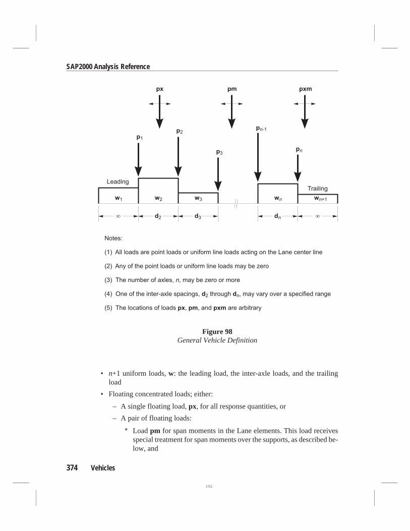
• n+1 uniform loads,w: the leading load, the inter-axle loads, and the trailingload
• Floating concentrated loads; either:
– A single floating load,px, for all response quantities, or
– A pair of floating loads:
∗ Loadpm for span moments in the Lane elements. This load receivesspecial treatment for span moments over the supports, as described be-low, and
374 Vehicles
SAP2000 Analysis Reference
Figure 98General Vehicle Definition
392

∗ Loadpxm for all response quantities except span moments in the Laneelements
• Whether or not this Vehicle is to be used for:
– “Negative” span moments over the supports in the Lane elements
– Vertical forces in interior piers and/or interior supports
– Response quantities other than the two types above
The number of axles,n, may be zero, in which case only a single uniform load andthe floating concentrated loads can be specified.
These parameters are illustrated in Figure 98 (page 374). Specific examples aregiven in the next subtopic using the standard Vehicles. Additional detail is providedin the following.
Moving the Vehicle
When a Vehicle is applied to a traffic Lane, the axles are moved along the length ofthe lane to where the maximum and minimum values are produced for every re-sponse quantity in every element. Usually this location will be different for each re-sponse quantity. For asymmetric (front to back) Vehicles, both directions of travelare considered.
Vehicle Response Categories
In order to satisfy certain requirements of the AASHTO HL design vehicular liveload (AASHTO, 1996 b), the available response quantities are divided into the fol-lowing categories:
(1) “Negative” span moments over the supports in Lane elements only. A “nega-tive” span moment is defined as that moment which causes tension in theupward-most face of a Lane element:
• Negative M3 if the local +2 axis is most upward (the default)
• Positive M3 if the local –2 axis is most upward
• Negative M2 if the local +3 axis is most upward
• Positive M2 if the local –3 axis is most upward
SAP2000 considers all “negative” span moments in the Lane elements to be inthis category without regard for the location of the supports (piers).
(2) Reactions at interior supports (piers). This takes two forms:
Vehicles 375
Chapter XVIII Bridge Analysis
393

• A compressive axial force in vertical Frame elements, where vertical is de-fined here as being within 15° of the Z axis
• The most upward local component of reactions and spring forces. For ex-ample:
– Positive F3 if the joint local +3 axis is most upward (the default)
– Negative F2 if the joint local –2 axis is most upward
The program automatically determines if these force components correspondto an interior support from the shape of the influence line. If the absolute mini-mum influence value does not occur at either end of the influence line, the sup-port is considered to be interior.
(3) All other response quantities not included in (1) and (2)
You may specify for each Vehicle whether or not to calculate each of these threecategories of response using the parameterssupmom, intsup, andother, respec-tively. Each of these parameters may take either value Y (yes) or N (no). The de-fault is Y for all three. This enables you to define different vehicles for the differentcategories of response. You must be sure that each category of response is capturedby at least one Vehicle in each Lane when defining the Moving Load cases.
Floating Concentrated Loads
The floating concentrated loads (px, pm, andpxm) are placed at the point of maxi-mum positive influence value (if any) and the point of minimum negative influencevalue (if any).
You may specify eitherpx, or the pairpm andpxm.
Floating loadpx is used equally for all response quantities.
Floating loadpm is only used for span moments in the Lane elements. A span mo-ments is defined as the moment in the most vertical local plane of a Lane element:
• M3 if the local 2 axis is most vertical (the default)
• M2 if the local 3 axis is most vertical
For “negative” span moments, as defined in category (1) under “Vehicle ResponseCategories” above, two floating concentrated loads of magnitudepm are located intwo different spans. This is used to meet the requirements of the AASHTO HS LaneLoad (AASHTO, 1996 a) for negative moments in continuous spans. The programautomatically determines the spans from the shape of the influence line by using the
376 Vehicles
SAP2000 Analysis Reference
394

two most negative influence values (if any) that are separated by at least one localmaximum. A single value ofpm is used for “positive” span moments.
Floating loadpxm is used for all response quantities except the span moments inthe Lane elements.
Standard Vehicles
The following standard vehicle types are available in SAP2000 to represent vehicu-lar live loads specified in various design codes. The type of vehicle is specified us-ing the parametertype.
Hn-44 and HSn-44
Vehicles specified withtype = Hn-44 andtype = HSn-44 represent the AASHTOstandard H and HS Truck Loads, respectively. Then in thetype is an integer scalefactor that specifies the nominal weight of the Vehicle in tons. Thus H15-44 is anominal 15 ton H Truck Load, and HS20-44 is a nominal 20 ton HS Truck Load.These Vehicles are illustrated in Figure 98 (page 378).
The effect of an H Vehicle is included in an HS Vehicle of the same nominalweight. If you are designing for both H and HS Vehicles, only the HS Vehicle isneeded.
Hn-44L and HSn-44L
Vehicles specified withtype = Hn-44L and type = HSn-44L represent theAASHTO standard H and HS Lane Loads, respectively. Then in thetype is an inte-ger scale factor that specifies the nominal weight of the Vehicle in tons. Thus H15-44 is a nominal 15 ton H Lane Load, and HS20-44 is a nominal 20 ton HS LaneLoad. These Vehicles are illustrated in Figure 98 (page 378). The Hn-44L andHSn-44L Vehicles are identical.
AML
Vehicles specified withtype = AML represent the AASHTO standard AlternateMilitary Load. This Vehicle consists of two 24 kip axles spaced 4 ft apart.
HL-93K, HL-93M and HL-93S
Vehicles specified withtype = HL-93K represent the AASHTO standard HL-93Load consisting of the code-specified design truck and the design lane load.
Vehicles 377
Chapter XVIII Bridge Analysis
395

378 Vehicles
SAP2000 Analysis Reference
Figure 99AASHTO Standard H and HS Vehicles
396

Vehicles 379
Chapter XVIII Bridge Analysis
Figure 100AASHTO Standard HL Vehicles
397

Vehicles specified withtype = HL-93M represent the AASHTO standard HL-93Load consisting of the code-specified design tandem and the design lane load.
Vehicles specified withtype = HL-93S represent the AASHTO standard HL-93Load consisting of two code-specified design trucks and the design lane load, allscaled by 90%. The axle spacing for each truck is fixed at 14 ft. The spacing be-tween the rear axle of the lead truck and the lead axle of the rear truck varies from50 ft to the length of the Lane. This vehicle is only used for negative moment oversupports and reactions at interior piers, sosupmom= Y, intsup = Y, andother = N.
A dynamic load allowance may be specified for each Vehicle using the parameterim. This is the additive percentage by which the concentrated truck or tandem axleloads will be increased. The uniform lane load is not affected. Thus ifim = 33, allconcentrated axle loads for the vehicle will be multiplied by the factor 1.33.
These Vehicles are illustrated in Figure 100 (page 379) forim = 0.
P5, P7, P9, P11, and P13
Vehicles specified withtype = P5,type = P7,type = P9,type = P11, andtype =P13 represent the Caltrans standard Permit Loads. These Vehicles are illustrated inFigure 100 (page 381).
The effect of a shorter Caltrans Permit Load is included in any of the longer PermitLoads. If you are designing for all of these permit loads, only the P13 Vehicle isneeded.
Cooper E 80
Vehicles specified withtype= COOPERE80 represent the AREA standard CooperE 80 train load. This Vehicle is illustrated in Figure 101 (page 382).
UICn
Vehicles specified withtype = UICn represent the European UIC (or British RU)train load. Then in thetype is an integer scale factor that specifies magnitude of theuniform load in kN/m. Thus UIC80 is the full UIC load with an 80 kN/m uniformload, and UIC60 is the UIC load with an 60 kN/m uniform load. The concentratedloads are not affected byn.
This Vehicle is illustrated in Figure 101 (page 382).
380 Vehicles
SAP2000 Analysis Reference
398

Vehicles 381
Chapter XVIII Bridge Analysis
Figure 101Caltrans Standard Permit Vehicles
399

382 Vehicles
SAP2000 Analysis Reference
Figure 102Standard Train Vehicles
400

RL
Vehicles specified withtype = RL represent the British RL train load. This Vehicleis illustrated in Figure 102 (page 382).
Vehicle ClassesThe designer is often interested in the maximum and minimum response of thebridge to the most extreme of several types of Vehicles rather than the effect of theindividual Vehicles. For this purpose, Vehicle Classes are defined that may includeany number of individual Vehicles. The maximum and minimum force and dis-placement response quantities for a Vehicle Class will be the maximum and mini-mum values obtained for any individual Vehicle in that Class. Only one Vehicleever acts at a time.
All Vehicle loads are applied to the traffic Lanes through the use of VehicleClasses. If it is desired to apply an individual Vehicle load, you must define a Vehi-cle Class that contains only that single Vehicle.
For example, the you may need to consider the most severe of a Truck Load and thecorresponding Lane Load, say the HS20-44 and HS20-44L loads. A Vehicle Classcan be defined to contain these two Vehicles. Additional Vehicles, such as the Al-ternate Military Load type AML, could be included in the Class as appropriate. Dif-ferent members of the Class may cause the most severe response at different loca-tions in the structure.
For HL-93 loading, you would first define three Vehicles, one each of the standardtypes HL-93K, HL-93M, and HL-93S. You then could define a single VehicleClass containing all three Vehicles.
Moving Load CasesThe final step in the definition of the vehicle live loading is the application of theVehicle Classes to the traffic Lanes. This is done by creating independentMovingLoad cases. Each Moving Load case consists of a set of assignments that specifyhow the Classes are assigned to the Lanes.
Eachassignmentin a Moving Load case requires the following data:
• A Vehicle Class,class
• A scale factor,sf, multiplying the effect ofclass(the default is unity)
Vehicle Classes 383
Chapter XVIII Bridge Analysis
401

• A list, lanes, of one or more Lanes in whichclassmay act (the default is allLanes)
• The minimum number,lmin , of Laneslanesin which classmust act (the de-fault is zero)
• The maximum number,lmax, of Laneslanesin which classmay act (the de-fault is all oflanes)
The program looks at all of the assignments in a Moving Load case, and tries everypossible permutation of loading the traffic Lanes with Vehicle Classes that is per-mitted by the assignments. No Lane is ever loaded by more than one Class at a time.
You may specify multiple-lane scale factors,rf1 , rf2 , rf3 , ..., for each Moving Loadcase that multiply the effect of each permutation depending upon the number ofloaded Lanes. For example, the effect of a permutation that loads two Lanes is mul-tiplied by rf2 .
The maximum and minimum response quantities for a Moving Load case will bethe maximum and minimum values obtained for any permutation permitted by theassignments. Usually the permutation producing the most severe response will bedifferent for different response quantities.
The results for a Moving Load case include the response due to loads ranging fromzero up to the specified Vehicle live loads. As a result, the envelope always includeszero response: the maximum will never be negative and the minimum will never bepositive. Thus there is no need to consider smaller vehicles that differ only by ascale factor. For example, the range of response for an HS20-44 vehicle includesthe response for an HS15-44 vehicle.
The concepts of assignment can be clarified with the help of the following exam-ples.
Example 1 — AASHTO HS Loading
Consider a four-lane bridge designed to carry AASHTO HS20-44 Truck and LaneLoads, and the Alternate Military Load (AASHTO, 1996 a). Suppose that it is re-quired that the number of Lanes loaded be that which produces the most severe re-sponse in every member. Only one of the three Vehicle loads is allowed per lane.Load intensities may be reduced by 10% and 25% when three or four Lanes areloaded, respectively.
Generally, loading all of the Lanes will produce the most severe moments andshears along the span and axial forces in the piers. However, the most severe torsion
384 Moving Load Cases
SAP2000 Analysis Reference
402

of the bridge deck and transverse bending of the piers will usually be produced byloading only those Lanes possessing eccentricities of the same sign.
Assume that the bridge structure and traffic Lanes have been defined. Three Vehi-cles are defined:
• name= HSK, type = HS20-44
• name= HSL, type = HS20-44L
• name= AML, type = AML
wherename is an arbitrary label assigned to each Vehicle. The three Vehicles areassigned to a single Vehicle Class, with an arbitrary label ofname= HS, so that themost severe of these three Vehicle loads will be used for every situation.
A single Moving Load case is then defined that seeks the maximum and minimumresponses throughout the structure for the most severe of loading all four Lanes,any three Lanes, any two Lanes or any single Lane. This can be accomplished usinga single assignment. The parameters for the assignment are:
• class= HS
• sf = 1
• lanes= 1, 2, 3, 4
• lmin = 1
• lmax = 4
The scale factors for the loading of multiple Lanes in the set of assignments arerf1= 1, rf2 = 1, rf3 = 0.9, andrf4 = 0.75.
There are fifteen possible permutations assigning the single Vehicle Class HS toany one, two, three, or four Lanes. These are presented in the following table:
Permutation Lane 1 Lane 2 Lane 3 Lane 4 Scale Factor
1 HS 1.00
2 HS 1.00
3 HS 1.00
4 HS 1.00
5 HS HS 1.00
Moving Load Cases 385
Chapter XVIII Bridge Analysis
403

Permutation Lane 1 Lane 2 Lane 3 Lane 4 Scale Factor
6 HS HS 1.00
7 HS HS 1.00
8 HS HS 1.00
9 HS HS 1.00
10 HS HS 1.00
11 HS HS HS 0.90
12 HS HS HS 0.90
13 HS HS HS 0.90
14 HS HS HS 0.90
15 HS HS HS HS 0.75
An “HS” in a Lane column of this table indicates application of Class HS; a blankindicates that the Lane is unloaded. The scale factor for each permutation is deter-mined by the number of Lanes loaded.
Example 2 — AASHTO HL Loading
Consider a four-lane bridge designed to carry AASHTO HL-93 loading(AASHTO, 1996 b). The approach is the same as used for AASHTO HS loading inthe previous example. Only the multiple-lane scale factors and the Vehicles differ.
Three Vehicles are defined:
• name= HLK, type = HL-93K
• name= HLM, type = HL-93M
• name= HLS, type = HL-93S
wherename is an arbitrary label assigned to each Vehicle.
The three Vehicles are assigned to a single Vehicle Class, with an arbitrary label ofname= HL, so that the most severe of these three Vehicle loads will be used forevery situation. By definition of the standard Vehicle type HL-93S, Vehicle HLSwill only be used when computing negative moments over supports or the reaction
386 Moving Load Cases
SAP2000 Analysis Reference
404

at interior piers. The other two Vehicles will be considered for all response quanti-ties.
A single Moving Load case is then defined that is identical to that of the previousexample, except thatclass= HL, and the scale factors for multiple Lanes arerf1 =1.2,rf2 = 1, rf3 = 0.85, andrf4 = 0.65.
There are again fifteen possible permutations assigning the single Vehicle ClassHL to any one, two, three, or four Lanes. These are similar to the permutations ofthe previous example, with the scale factors changed as appropriate.
Example 3 — Caltrans Permit Loading
Consider the four-lane bridge of the previous examples now subject to CaltransCombination GroupIPW (Caltrans, 1995). Here the permit load(s) are to be usedalone in a single traffic Lane, or in combination with one HS or Alternate MilitaryLoad in a separate traffic lane, depending upon which is more severe.
Four Vehicles are defined:
• name= HSK, type = HS20-44
• name= HSL, type = HS20-44L
• name= AML, type = AML
• name= P13,type = P13
wherename is an arbitrary label assigned to each Vehicle.
The first three Vehicles are assigned to a Vehicle Class that is given the labelname= HS, as in Example 1. The last Vehicle is assigned as the only member of a VehicleClass that is given the labelname= P13. Note that the effects of SAP2000 Vehicletypes P5, P7, P9, and P11 are captured by Vehicle type P13.
Combination GroupIPW is then represented as a single Moving Load case consist-ing of the assignment of Class P13 to any single Lane with or without Class HS be-ing assigned to any other single Lane. This can be accomplished using two assign-ments. A scale factor of unity is used regardless of the number of loaded Lanes.
The first assignment assigns Class P13 to any single Lane:
• class= P13
• sf = 1
• lanes= 1, 2, 3, 4
Moving Load Cases 387
Chapter XVIII Bridge Analysis
405

• lmin = 1
• lmax = 1
The second assignment assigns Class HS to any single Lane, or to no Lane at all:
• class= HS
• sf = 1
• lanes= 1, 2, 3, 4
• lmin = 0
• lmax = 1
There are sixteen possible permutations for these two assignments such that noLane is loaded by more than one Class at a time. These are presented in the follow-ing table:
Permutation Lane 1 Lane 2 Lane 3 Lane 4 Scale Factor
1 P 1.00
2 P HS 1.00
3 P HS 1.00
4 P HS 1.00
5 HS P 1.00
6 P 1.00
7 P HS 1.00
8 P HS 1.00
9 HS P 1.00
10 HS P 1.00
11 P 1.00
12 P HS 1.00
13 HS P 1.00
14 HS P 1.00
388 Moving Load Cases
SAP2000 Analysis Reference
406

Permutation Lane 1 Lane 2 Lane 3 Lane 4 Scale Factor
15 HS P 1.00
16 P 1.00
Example 4 — Restricted Caltrans Permit Loading
Consider the four-Lane bridge and the Caltrans permit loading of Example 3, butsubject to the following restrictions:
• The permit Vehicle is only allowed in Lane 1 or Lane 4
• The Lane adjacent to the Lane occupied by the permit Vehicle must be empty
Two Moving Load cases are required, each containing two assignments. A scalefactor of unity is used regardless of the number of loaded Lanes.
The first Moving Load case considers the case where the permit Vehicle occupiesLane 1. The first assignment assigns Class P13 to Lane 1
• class= P13
• sf = 1
• lanes= 1
• lmin = 1
• lmax = 1
The second assignment assigns Class HS to either Lane 3 or 4, or to no Lane at all:
• class= HS
• sf = 1
• lanes= 3, 4
• lmin = 0
• lmax = 1
These assignments permits the following three permutations:
Moving Load Cases 389
Chapter XVIII Bridge Analysis
407
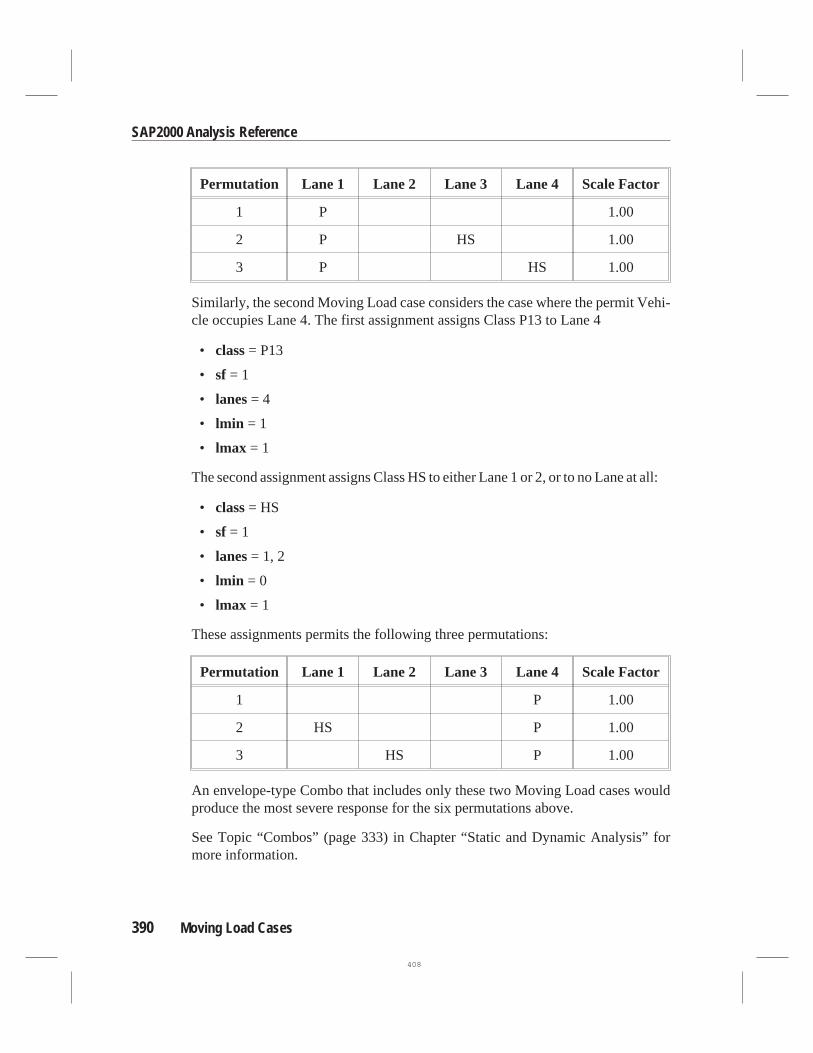
Permutation Lane 1 Lane 2 Lane 3 Lane 4 Scale Factor
1 P 1.00
2 P HS 1.00
3 P HS 1.00
Similarly, the second Moving Load case considers the case where the permit Vehi-cle occupies Lane 4. The first assignment assigns Class P13 to Lane 4
• class= P13
• sf = 1
• lanes= 4
• lmin = 1
• lmax = 1
The second assignment assigns Class HS to either Lane 1 or 2, or to no Lane at all:
• class= HS
• sf = 1
• lanes= 1, 2
• lmin = 0
• lmax = 1
These assignments permits the following three permutations:
Permutation Lane 1 Lane 2 Lane 3 Lane 4 Scale Factor
1 P 1.00
2 HS P 1.00
3 HS P 1.00
An envelope-type Combo that includes only these two Moving Load cases wouldproduce the most severe response for the six permutations above.
See Topic “Combos” (page 333) in Chapter “Static and Dynamic Analysis” formore information.
390 Moving Load Cases
SAP2000 Analysis Reference
408

Influence Line ToleranceSAP2000 simplifies the influence lines used for response calculation in order to in-crease efficiency. A relative tolerance is used to reduce the number of load pointsby removing those that are approximately duplicated or that can be approximatelylinearly-interpolated. The default value of this tolerance permits response errors onthe order of 0.01%. Setting the tolerance to zero will provide exact results to withinthe resolution of the analysis.
Exact and Quick Response CalculationFor the purpose of moving a Vehicle along a lane, each axle is placed on every loadpoint in turn. When another axle falls between two load points, the effect of thataxle is determined by linear interpolation of the influence values. The effect of uni-form loads is computed by integrating the linearly-interpolated segments of the in-fluence line. This method is exact to within the resolution of the analysis, but iscomputationally intensive if there are many load points.
A “Quick” method is available which may be much faster than the usual “Exact”method, but it may also be less accurate. The Quick method approximates the influ-ence line by using a limited number of load points in each “span.” For purposes ofthis discussion, a span is considered to be a region where the influence line is allpositive or all negative.
The degree of approximation to be used is specified by the parameterquick, whichmay be any non-negative integer. The default value isquick = 0, which indicates touse the full influence line, i.e., the Exact method.
Positive values indicate increasing degrees of refinement for the Quick method. Forquick = 1, the influence line is simplified by using only the maximum or minimumvalue in each span, plus the zero points at each end of the span. Forquick = 2, an ad-ditional load point is used on either side of the maximum/minimum. Higher degreesof refinement use additional load points. The number of points used in a span can beas many as 2quick+1, but not more than the number of load points available in thespan for the Exact method.
It is strongly recommended thatquick = 0 be used for all final analyses. For pre-liminary analyses,quick = 1, 2, or 3 is usually adequate, withquick = 2 often pro-viding a good balance between speed and accuracy. The effect of parameterquickupon speed and accuracy is problem-dependent, and you should experiment to de-termine the best value to use for each different model.
Influence Line Tolerance 391
Chapter XVIII Bridge Analysis
409
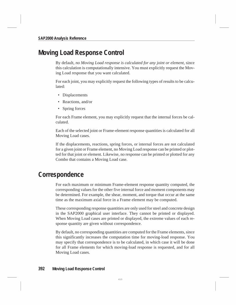
Moving Load Response ControlBy default,no Moving Load response is calculated for any joint or element, sincethis calculation is computationally intensive. You must explicitly request the Mov-ing Load response that you want calculated.
For each joint, you may explicitly request the following types of results to be calcu-lated:
• Displacements
• Reactions, and/or
• Spring forces
For each Frame element, you may explicitly request that the internal forces be cal-culated.
Each of the selected joint or Frame-element response quantities is calculated for allMoving Load cases.
If the displacements, reactions, spring forces, or internal forces are not calculatedfor a given joint or Frame element, no Moving Load response can be printed or plot-ted for that joint or element. Likewise, no response can be printed or plotted for anyCombo that contains a Moving Load case.
CorrespondenceFor each maximum or minimum Frame-element response quantity computed, thecorresponding values for the other five internal force and moment components maybe determined. For example, the shear, moment, and torque that occur at the sametime as the maximum axial force in a Frame element may be computed.
These corresponding response quantities are only used for steel and concrete designin the SAP2000 graphical user interface. They cannot be printed or displayed.When Moving Load cases are printed or displayed, the extreme values of each re-sponse quantity are given without correspondence.
By default, no corresponding quantities are computed for the Frame elements, sincethis significantly increases the computation time for moving-load response. Youmay specify that correspondence is to be calculated, in which case it will be donefor all Frame elements for which moving-load response is requested, and for allMoving Load cases.
392 Moving Load Response Control
SAP2000 Analysis Reference
410

Computational ConsiderationsThe computation of influence lines requires a moderate amount of computer timeand a large amount of disk storage compared with the execution of other typicalSAP2000 analyses. The amount of computer time is approximately proportional toN2L, whereN is the number of structure degrees-of-freedom, andL is the number ofload points. The amount of disk storage required is approximately proportional toNL.
Increasing the resolution of the analysis by increasing the number of Frame ele-ments (holdingnsegconstant) causes approximately proportional increases inNandL, and hence increases computation time by aboutL3 and storage space by aboutL2. Holding the number of elements constant and increasingnseginstead increasescomputation time and storage space each by approximatelyL. Clearly the lattermethod is more efficient.
If all traffic Lanes have zero eccentricities everywhere, computation time and stor-age space for the influence lines are cut in half.
The computation of Moving Load response may require a large amount of com-puter time compared with the execution of other typical SAP2000 analyses. Theamount of disk storage needed (beyond the influence lines) is small.
The computation time for Moving Load response is proportional to the number ofresponse points. To obtain the same effective increase in resolution, increasing thevalues ofnsegproduces fewer additional response points than does increasing thenumber of elements, since the latter approach introduces duplicate response pointsat the joints. Hence changingnsegis more efficient. Considerable savings in com-putation time can also be realized by restricting Moving Load calculations to onlythose joints and Frame elements of significant interest.
The computation time for Moving Load response is also directly proportional to thenumber of Lanes. It is not, however, sensitive to whether or not Lane eccentricitiesare present.
For each Vehicle load, the computation time is approximately proportional to thesquare of the number of axles. It is also proportional toL¢, the effective number ofload points. Larger values of the truck influence tolerance tend to produce smallervalues ofL¢ compared toL. The value ofL¢ will be different for each response quan-tity; it tends to be smaller for structures with simple spans than with continuousspans. The value ofL¢ is not sensitive to whether increases in resolution are ob-tained by increasing the number of elements or the number of output segments.
Computational Considerations 393
Chapter XVIII Bridge Analysis
411

394 Computational Considerations
SAP2000 Analysis Reference
412

C h a p t e r XIX
The Output Files
Three output text files are produced during a SAP2000 analysis: the input echo file,the analysis log file, and the results output file. Additional output may be obtainedusing the SAP2000 graphical user interface.
Basic Topics for All Users
• Overview
• The Input Echo (.EKO) File
• The Analysis Log (.LOG) File
• The Results Output (.OUT) File
Advanced Topics
• Element Joint Force Output
• Joint and Element Output Control
• Pagination Control
395
413

OverviewAn analysis performed by SAP2000 produces three output text files. These are:
• The input echo file, having file extension .EKO; this is a tabulation of the inputdata text file as read and checked by the analysis
• The analysis log file, having file extension .LOG; this contains analysis statis-tics, warnings, and error messages
• The results output file, having file extension .OUT; this contains displace-ments, forces, stresses and other results of the analysis
When importing a SAP90 or SAP2000 input data text file, only the input echo file isproduced.
For an input data file named EXAMPLE.SDB or EXAMPLE.S2K, these fileswould be called EXAMPLE.EKO, EXAMPLE.LOG, and EXAMPLE.OUT, re-spectively.
These are ASCII text files with an 80-character wide output format. Smaller filesmay be viewed with a text editor such as Windows Notepad, or any other editor orword-processing program in text mode. For larger problems, you may need to use alarge-capacity editor or word-processing program. You may use any standard Win-dows printer to print these files.
The Input Echo (.EKO) FileThe input echo file, more simply called theecho file, is created during the data-checking phase of the program. It contains a tabulation of the input data file as readand interpreted by SAP2000, as well as the details of any warnings or errors de-tected during this phase. The contents of this file are self-explanatory.
It is recommended that you carefully review the contents of the echo file for errors,warnings, and the correctness of the model.
If errors are present, the analysis phase of the program will not be executed. Themodel must be corrected and the program executed again.
If only warnings are present, the analysis phase may proceed. You should checkthese warnings carefully before reviewing the results of the analysis.
All data that is used by the analysis phase is presented in the input echo file. Assuch, this file forms a record of the analysis being performed.
396 Overview
SAP2000 Analysis Reference
414

The Analysis Log (.LOG) FileTheanalysis log file, more simply called thelog file, is created during the analysisphase of the program. It contains analysis statistics and results summaries, as wellas the details of any warnings or errors detected during this phase.
It is strongly recommendedthat you carefully review the contents of the log file forerrors, warnings, and the results summaries, including the global force balance rela-tive errors.
If errorsare present, the analysis phase of the program will have terminated beforecompletion. If onlywarningsare present, the analysis phase should have com-pleted. In either case, you should check these errors and warnings carefully beforeexamining the results of the analysis.
The analysis phase is divided into many sub-phases. The time and date at the begin-ning and end of each of these sub-phases is reported. The date is given inyear/month/day format, and the time is given in hour:minute:second format.
The following additional information is provided in the analysis log file:
• The amount of memory allocated for data storage, in bytes
• The number of elements formed
• The number of Welds and Constraints formed
• The number of equations formed, the size of the stiffness matrix, and thenumber of loads solved
• The number of natural frequencies of the model below frequencycyc if har-monic steady-state analysis is performed; see Topic “Harmonic Steady-StateAnalysis” (page 294) in Chapter “Static and Dynamic Analysis” for more in-formation
• The number of natural frequencies of the model below frequencyshift if eigen-vector analysis is performed with a frequency shift; see Topic “EigenvectorAnalysis” (page 296) in Chapter “Static and Dynamic Analysis” for more in-formation
• For modal analysis, the control parameters and the number of Modes found
• For eigenvector analysis, the number of iterations performed
• For Ritz-vector analysis, the number of generation cycles performed and thereasons for discarding the starting load vectors (if any)
• For response-spectrum analysis, the number of analyses performed
The Analysis Log (.LOG) File 397
Chapter XIX The Output Files
415

398 The Analysis Log (.LOG) File
SAP2000 Analysis Reference
------------------------------------------------------- 1996/02/01 16:36:51.06
MEMORY AVAILABLE FOR DATA (BYTES) = 2000000
------------------------------------------------------- 1996/02/01 16:36:51.17
J O I N T E L E M E N T F O R M A T I O N P H A S E
NUMBER OF JOINT ELEMENTS FORMED = 14NUMBER OF SPRING ELEMENTS FORMED = 0
------------------------------------------------------- 1996/02/01 16:36:51.66
F R A M E E L E M E N T F O R M A T I O N P H A S E
NUMBER OF FRAME ELEMENTS FORMED = 35
------------------------------------------------------- 1996/02/01 16:36:53.75
E Q U A T I O N F O R M A T I O N A N D S O L U T I O N P H A S E
TOTAL NUMBER OF EQUILIBRIUM EQUATIONS = 49APPROXIMATE “EFFECTIVE” BAND WIDTH = 8
NUMBER OF EQUATION STORAGE BLOCKS = 1MAXIMUM BLOCK SIZE (NUMBER OF TERMS) = 418SIZE OF STIFFNESS FILE (BYTES) = 3556
NUMBER OF EQUATIONS TO REDUCE = 49NUMBER OF LOAD CONDITIONS TO SOLVE = 2
------------------------------------------------------- 1996/02/01 16:36:58.09
J O I N T O U T P U T P H A S E
G L O B A L F O R C E B A L A N C E R E L A T I V E E R R O R S
PERCENT FORCE AND MOMENT ERROR AT THE ORIGIN, IN GLOBAL COORDINATES
LOAD FX FY FZ MX MY MZ1 .000000 7.38E-17 4.72E-14 6.62E-15 .000000 .0000002 .000000 9.97E-16 7.98E-15 2.50E-14 .000000 .000000
COMB FX FY FZ MX MY MZ1 .000000 7.38E-17 4.84E-14 1.67E-14 .000000 .000000
------------------------------------------------------- 1996/02/01 16:37:02.54
F R A M E E L E M E N T O U T P U T P H A S E
NUMBER OF FRAME ELEMENTS SAVED = 35NUMBER OF FRAME ELEMENTS PRINTED = 35
------------------------------------------------------- 1996/02/01 16:37:04.62
...Output Edited for Brevity...
Figure 103Typical Contents of the Analysis Log (.LOG) File
416

• For each time-history analysis, the control parameters and the number of timesteps completed
• For each nonlinear time-history analysis, the number of substeps and iterationscompleted and other statistics
• For moving-load analysis, the control parameters and solution statistics
• The global force balance relative errors; see Topic “Global Force Balance Out-put” (page 107) in Chapter “Joints and Degrees of Freedom” for more informa-tion
• The number of elements processed for output
Typical output is shown in Figure 103 (page 398).
The Results Output (.OUT) FileThe results output file, more simply called theoutput file , is created during theanalysis phase of the program. The results given for the joints and elements are sub-ject to your control. See Topic “Joint and Element Output Control” (page 405) inthis chapter for more information. The remaining results are always given by theprogram when appropriate.
It is recommended that you carefully review the input echo (.EKO) file and theanalysis log (.LOG) file for errors, warnings, and correctness of the model beforelooking at the results output file.
The output file does not contain any warnings or error messages.
The results in the output file are divided into various sections, each with a headingthat describes the type of results that follow. These sections are described below inthe same order that they appear in the output file:
• The following output section is present if there are any Body, Diaphragm,Plate, Rod, and Beam Constraints that constrain more than two joints:
CONSTRAINT COORDINATES AND MASSES
See Topic “Constraint Output” (page 133) in Chapter “Constraints and Welds.”
• The following output section is always present:
DISPLACEMENT DEGREES OF FREEDOM
The Results Output (.OUT) File 399
Chapter XIX The Output Files
417

See Topic “Degree of Freedom Output” (page 97) in Chapter “Joints and De-grees of Freedom.”
• The following output sections are present if the structure has any mass:
ASSEMBLED JOINT MASSES
TOTAL UNRESTRAINED MASS AND LOCATION
See Topic “Joint Mass Output” (page 98) in Chapter “Joints and Degrees ofFreedom.”
• The following output sections are present if an eigenvector or Ritz-vector mo-dal analysis has been performed:
MODAL PERIODS AND FREQUENCIES
MODAL PARTICIPATION FACTORS
MODAL PARTICIPATING MASS RATIOS
MODAL LOAD PARTICIPATION RATIOS
See Topic “Modal Analysis Output” (page 303) in Chapter “Static and Dy-namic Analysis.”
• The following output sections are present if response-spectrum analyses havebeen performed:
RESPONSE SPECTRUM ACCELERATIONS
RESPONSE SPECTRUM MODAL AMPLITUDES
RESPONSE SPECTRUM MODAL CORRELATIONS
RESPONSE SPECTRUM BASE REACTIONS
See Topic “Response-Spectrum Analysis Output” (page 317) in Chapter“Static and Dynamic Analysis.”
• The following output section is present whenever joint displacements are re-quested:
JOINT DISPLACEMENTS
See Topic “Joint Displacement Output” (page 100) in Chapter “Joints and De-grees of Freedom.”
400 The Results Output (.OUT) File
SAP2000 Analysis Reference
418

• The following output sections are present whenever joint applied loads are re-quested and the corresponding loads exist:
APPLIED LOADS
INERTIAL LOADS
See Topic “Force Output” (page 102) in Chapter “Joints and Degrees of Free-dom.”
• The following output sections are present whenever joint reactions are re-quested and the corresponding types of forces exist:
SPRING FORCES
NLLINK FORCES
RESTRAINT FORCES (REACTIONS)
CONSTRAINT FORCES
See Topic “Force Output” (page 102) in Chapter “Joints and Degrees of Free-dom.”
• The following output section is always present:
GLOBAL FORCE BALANCE
See Topic “Global Force Balance Output” (page 107) in Chapter “Joints andDegrees of Freedom.”
• The following output sections are present whenever joint forces are requestedfor the corresponding type of element:
FRAME ELEMENT JOINT FORCES
SHELL ELEMENT JOINT FORCES
PLANE ELEMENT JOINT FORCES
ASOLID ELEMENT JOINT FORCES
SOLID ELEMENT JOINT FORCES
NLLINK ELEMENT JOINT FORCES
See Topic “Joint Force Output” (page 402) in this chapter.
See Topic “Joint Force Output” (page 179) in Chapter “The Frame Element.”
See Topic “Joint Force Output” (page 203) in Chapter “The Shell Element.”
See Topic “Joint Force Output” (page 216) in Chapter “The Plane Element.”
The Results Output (.OUT) File 401
Chapter XIX The Output Files
419

See Topic “Joint Force Output” (page 231) in Chapter “The Asolid Element.”
See Topic “Joint Force Output” (page 241) in Chapter “The Solid Element.”
See Topic “Joint Force Output” (page 277) in Chapter “The Nllink Element.”
• The following output sections are present whenever internal forces or stressesare requested for the corresponding type of element:
FRAME ELEMENT INTERNAL FORCES
SHELL ELEMENT INTERNAL FORCES & STRESSES
PLANE ELEMENT STRESSES
ASOLID ELEMENT STRESSES
SOLID ELEMENT STRESSES
NLLINK ELEMENT INTERNAL FORCES & DEFORMS
See Topic “Internal Force Output” (page 176) in Chapter “The Frame Ele-ment.”
See Topic “Internal Force and Stress Output” (page 198) in Chapter “The ShellElement.”
See Topic “Stress Output” (page 215) in Chapter “The Plane Element.”
See Topic “Stress Output” (page 230) in Chapter “The Asolid Element.”
See Topic “Stress Output” (page 240) in Chapter “The Solid Element.”
See Topic “Internal Force and Deformation Output” (page 275) in Chapter“The Nllink Element.”
Typical output is shown in the respective topics referenced above.
Element Joint Force OutputTheelement joint forcesare concentrated forces and moments acting at the jointsof the element that represent the effect of the rest of the structure upon the elementand that cause the deformation of the element. The moments will always be zero forthe solid-type elements: Plane, Asolid, and Solid.
A positive value of force or moment tends to cause a positive value of translation orrotation of the element along the corresponding joint degree of freedom. See Figure104 (page 403).
402 Element Joint Force Output
SAP2000 Analysis Reference
420

Element Joint Force Output 403
Chapter XIX The Output Files
Figure 104Element Joint Forces when All Joints Have the Global Coordinate System for
Their Local Coordinate Systems
421

Element joint forces must not be confused with internal forces and moments which,like stresses, actwithin the volume of the element.
For a given element, the vector of element joint forces,f, is computed as:
f K u r= −
whereK is the element stiffness matrix,u is the vector of element joint displace-ments, andr is the vector of element applied loads as apportioned to the joints. Theapplied loads may include Force, Self-Weight, Gravity, Concentrated Span, Dis-tributed Span, Uniform, Surface Pressure, Pore Pressure, Temperature, Prestress,and Rotate Loads, as appropriate, that act directly on the given element.
The element joint forces are always referred to the local axes of the individualjoints. They are identified in the output as F1, F2, F3, M1, M2, and M3. However, ifall joints use the global coordinate system as the local system (the usual situation),then the forces and moments are identified as FX, FY, FZ, MX, MY, and MZ.
Element joint forces and moments for the different types of elements are printed inthe output file under the headings:
FRAME ELEMENT JOINT FORCES
SHELL ELEMENT JOINT FORCES
PLANE ELEMENT JOINT FORCES
ASOLID ELEMENT JOINT FORCES
SOLID ELEMENT JOINT FORCES
NLLINK ELEMENT JOINT FORCES
All joint forces for a single element are printed together. Elements of a given typeare presented in alpha-numeric order. For each Analysis Case the joint forces areprinted at all element joints.
Typical element joint force output is shown for the Frame element in Figure 105(page 406), the Shell element in Figure 106 (page 407), the Plane element in Figure107 (page 408), the Asolid element in Figure 108 (page 409), the Solid element inFigure 109 (page 410), and the Nllink element in Figure 110 (page 411).
By default, no element joint forces are printed. You may specify which AnalysisCases are to be printed for each element. Available Analysis Cases include Loads,
404 Element Joint Force Output
SAP2000 Analysis Reference
422

Modes, Specs, and Combos, but not Histories, Moving Loads, or Combos that con-tain Histories or Moving Loads.
The element joint forces are available through the SAP2000 graphical user inter-face using the “Group Joint Force Sum.” This sum is the resultant of the forces andmoments acting on one or more joints of one or more elements.
It is important to note that the Response Spectrum results are always positive, andthat the correspondence between different values has been lost.
For more information:
• See Topic “Joint and Element Output Control” (page 405) in this chapter
• Chapter “The Frame Element” (page 145)
• Chapter “The Shell Element” (page 181)
• Chapter “The Plane Element” (page 205)
• Chapter “The Asolid Element” (page 219)
• Chapter “The Solid Element” (page 233)
• Chapter “The Nllink Element” (page 243)
Joint and Element Output ControlBy default, no joint and element results are written to the results output (.OUT) file.
You may select the types of analysis results to be printed for each of the followinganalysis cases:
• Load Cases
• Modes
• Specs
• Histories
• Moving Loads
• Combos
The printed History results are just the maximum and minimum values of each re-sponse quantity attained during the History. For the time-variation of the response,use the SAP2000 graphical user interface.
Joint and Element Output Control 405
Chapter XIX The Output Files
423

406 Joint and Element Output Control
SAP2000 Analysis Reference
F R A M E E L E M E N T J O I N T F O R C E S
FORCES AND MOMENTS ACTING ON ELEMENTS, IN GLOBAL COORDINATES
ELEM 1 ==================
LOAD 1 ------------------
JOINT FX FY FZ MX MY MZ33 -7.35E-13 9.73E-11 1000.000 -72000.000 -2026.122 1.35E-1235 7.35E-13 -9.73E-11 -1000.000 84000.000 2026.122 7.47E-12
SPEC SPEC ------------------
JOINT FX FY FZ MX MY MZ33 0.972230 126.377896 68.323489 3190.341 89.135262 1.87825235 0.972230 126.377896 68.323489 3978.697 89.135262 9.788509
COMB BOTH ------------------ MAX
JOINT FX FY FZ MX MY MZ33 0.972230 126.377896 1068.323 -68809.659 -1936.987 1.87825235 0.972230 126.377896 -931.676511 87978.697 2115.257 9.788509
COMB BOTH ------------------ MIN
JOINT FX FY FZ MX MY MZ33 -0.972230 -126.377896 931.676511 -75190.341 -2115.257 -1.87825235 -0.972230 -126.377896 -1068.323 80021.303 1936.987 -9.788509
ELEM 2 ==================
LOAD 1 ------------------
JOINT FX FY FZ MX MY MZ34 7.35E-13 9.73E-11 1000.000 -72000.000 2026.122 -1.35E-1236 -7.35E-13 -9.73E-11 -1000.000 84000.000 -2026.122 -7.47E-12
SPEC SPEC ------------------
JOINT FX FY FZ MX MY MZ34 0.972230 126.377896 68.323489 3190.341 89.135262 1.87825236 0.972230 126.377896 68.323489 3978.697 89.135262 9.788509
COMB BOTH ------------------ MAX
JOINT FX FY FZ MX MY MZ34 0.972230 126.377896 1068.323 -68809.659 2115.257 1.87825236 0.972230 126.377896 -931.676511 87978.697 -1936.987 9.788509
COMB BOTH ------------------ MIN
JOINT FX FY FZ MX MY MZ34 -0.972230 -126.377896 931.676511 -75190.341 1936.987 -1.87825236 -0.972230 -126.377896 -1068.323 80021.303 -2115.257 -9.788509
...Output Edited for Brevity...
Figure 105Frame Element Joint Forces in the Output File
424

Joint and Element Output Control 407
Chapter XIX The Output Files
S H E L L E L E M E N T J O I N T F O R C E S
FORCES AND MOMENTS ACTING ON ELEMENTS, IN GLOBAL COORDINATES
ELEM 1 ==================
LOAD 1 ------------------
JOINT FX FY FZ MX MY MZ10 6.28E-27 9.73E-11 1000.000 -48000.000 9.92E-11 1.31E-1231 -1.86E-13 -9.73E-11 -1000.000 60000.000 -641.113050 1.32E-1225 1.49E-27 9.73E-11 1000.000 -48000.000 -2.86E-10 -1.31E-1232 1.86E-13 -9.73E-11 -1000.000 60000.000 641.113050 -1.32E-12
SPEC SPEC ------------------
JOINT FX FY FZ MX MY MZ10 0.485709 107.747660 61.665399 1718.664 6.42E-13 1.81857631 1.320783 107.748554 61.665399 2429.634 33.426016 1.83578225 0.484206 107.746818 61.665399 1718.664 1.79E-12 1.81579432 1.322272 107.745924 61.665399 2429.634 33.426016 1.831400
COMB BOTH ------------------ MAX
JOINT FX FY FZ MX MY MZ10 0.485709 107.747660 1061.665 -46281.336 9.99E-11 1.81857631 1.320783 107.748554 -938.334601 62429.634 -607.687034 1.83578225 0.484206 107.746818 1061.665 -46281.336 -2.85E-10 1.81579432 1.322272 107.745924 -938.334601 62429.634 674.539066 1.831400
COMB BOTH ------------------ MIN
JOINT FX FY FZ MX MY MZ10 -0.485709 -107.747660 938.334601 -49718.664 9.86E-11 -1.81857631 -1.320783 -107.748554 -1061.665 57570.366 -674.539066 -1.83578225 -0.484206 -107.746818 938.334601 -49718.664 -2.88E-10 -1.81579432 -1.322272 -107.745924 -1061.665 57570.366 607.687034 -1.831400
ELEM 2 ==================
LOAD 1 ------------------
JOINT FX FY FZ MX MY MZ31 1.86E-13 9.73E-11 1000.000 -60000.000 641.113050 -1.32E-1233 7.35E-13 -9.73E-11 -1000.000 72000.000 2026.122 -1.35E-1232 -1.86E-13 9.73E-11 1000.000 -60000.000 -641.113050 1.32E-1234 -7.35E-13 -9.73E-11 -1000.000 72000.000 -2026.122 1.35E-12
SPEC SPEC ------------------
JOINT FX FY FZ MX MY MZ31 0.584210 120.062949 66.239113 2429.634 33.426016 1.83357833 0.235931 120.062949 66.239113 3190.341 89.135262 1.87825232 0.584210 120.062949 66.239113 2429.634 33.426016 1.83357834 0.235931 120.062949 66.239113 3190.341 89.135262 1.878252
...Output Edited for Brevity...
Figure 106Shell Element Joint Forces in the Output File
425

408 Joint and Element Output Control
SAP2000 Analysis Reference
P L A N E E L E M E N T J O I N T F O R C E S
FORCES AND MOMENTS ACTING ON ELEMENTS, IN GLOBAL COORDINATES
ELEM 1 ==================
LOAD 1 ------------------
JOINT FX FY FZ MX MY MZ1 .000000 -4.04E-11 167.000000 .000000 .000000 .0000002 .000000 6.17E-11 -1.03E-10 .000000 .000000 .0000003 0.000108 2000.000 -127.672098 .000000 .000000 .0000006 .000000 -1.08E-10 666.000000 .000000 .000000 .0000007 .000000 6.90E-11 3.92E-10 .000000 .000000 .0000008 3.09E-18 4.15E-11 -744.655804 .000000 .000000 .000000
11 .000000 -1.78E-11 167.000000 .000000 .000000 .00000012 .000000 1.43E-11 -1.35E-10 .000000 .000000 .00000013 -0.000108 -2000.000 -127.672098 .000000 .000000 .000000
SPEC SPEC ------------------
JOINT FX FY FZ MX MY MZ1 .000000 2.095103 1.960365 .000000 .000000 .0000002 .000000 6.736706 4.555885 .000000 .000000 .0000003 3.00E-06 45.955743 3.475362 .000000 .000000 .0000006 .000000 6.792403 6.514757 .000000 .000000 .0000007 .000000 21.085504 14.519078 .000000 .000000 .0000008 5.36E-07 24.347802 26.751296 .000000 .000000 .000000
11 .000000 2.095289 1.960390 .000000 .000000 .00000012 .000000 6.737990 4.555878 .000000 .000000 .00000013 3.00E-06 45.955810 3.475244 .000000 .000000 .000000
ELEM 2 ==================
LOAD 1 ------------------
JOINT FX FY FZ MX MY MZ16 .000000 -4.04E-11 167.000000 .000000 .000000 .00000017 .000000 6.17E-11 -1.03E-10 .000000 .000000 .00000018 -0.000108 2000.000 -127.672098 .000000 .000000 .00000021 .000000 -1.08E-10 666.000000 .000000 .000000 .00000022 .000000 6.90E-11 3.92E-10 .000000 .000000 .00000023 -3.09E-18 4.15E-11 -744.655804 .000000 .000000 .00000026 .000000 -1.78E-11 167.000000 .000000 .000000 .00000027 .000000 1.43E-11 -1.35E-10 .000000 .000000 .00000028 0.000108 -2000.000 -127.672098 .000000 .000000 .000000
...Output Edited for Brevity...
Figure 107Plane Element Joint Forces in the Output File
426

Joint and Element Output Control 409
Chapter XIX The Output Files
A S O L I D E L E M E N T J O I N T F O R C E S
FORCES AND MOMENTS ACTING ON ELEMENTS, IN GLOBAL COORDINATES
ELEM 1 ==================
LOAD INTPRES ------------------
JOINT FX FY FZ MX MY MZ1 2.93E-14 -0.060041 .000000 .000000 .000000 .0000002 -4.98E-15 0.084594 .000000 .000000 .000000 .0000003 -0.035999 -0.056720 .000000 .000000 .000000 .000000
12 -5.95E-14 -9.15E-15 .000000 .000000 .000000 .00000013 -1.96E-13 -9.98E-14 .000000 .000000 .000000 .00000014 -0.143192 1.38E-14 .000000 .000000 .000000 .00000023 -1.69E-14 0.060041 .000000 .000000 .000000 .00000024 -4.04E-14 -0.084594 .000000 .000000 .000000 .00000025 -0.035999 0.056720 .000000 .000000 .000000 .000000
LOAD LOGTEMP ------------------
JOINT FX FY FZ MX MY MZ1 4.55E-13 13.546107 .000000 .000000 .000000 .0000002 1.36E-12 16.192718 .000000 .000000 .000000 .0000003 -0.746624 12.833193 .000000 .000000 .000000 .000000
12 -3.64E-12 3.47E-13 .000000 .000000 .000000 .00000013 -3.75E-12 -5.54E-13 .000000 .000000 .000000 .00000014 -3.173884 3.53E-12 .000000 .000000 .000000 .00000023 -1.36E-12 -13.546107 .000000 .000000 .000000 .00000024 1.34E-12 -16.192718 .000000 .000000 .000000 .00000025 -0.746624 -12.833193 .000000 .000000 .000000 .000000
ELEM 2 ==================
LOAD INTPRES ------------------
JOINT FX FY FZ MX MY MZ3 0.035999 -0.099947 .000000 .000000 .000000 .0000004 -3.80E-14 0.138916 .000000 .000000 .000000 .0000005 -0.028017 -0.093595 .000000 .000000 .000000 .000000
14 0.143192 -3.29E-14 .000000 .000000 .000000 .00000015 -1.44E-13 8.16E-14 .000000 .000000 .000000 .00000016 -0.110260 1.34E-13 .000000 .000000 .000000 .00000025 0.035999 0.099947 .000000 .000000 .000000 .00000026 -9.38E-15 -0.138916 .000000 .000000 .000000 .00000027 -0.028017 0.093595 .000000 .000000 .000000 .000000
...Output Edited for Brevity...
Figure 108Asolid Element Joint Forces in the Output File
427

410 Joint and Element Output Control
SAP2000 Analysis Reference
S O L I D E L E M E N T J O I N T F O R C E S
FORCES AND MOMENTS ACTING ON ELEMENTS, IN GLOBAL COORDINATES
ELEM 1 ==================
LOAD 1 ------------------
JOINT FX FY FZ MX MY MZ3 5.27E-12 -2000.000 127.672098 .000000 .000000 .000000
18 3.77E-12 -2000.000 127.672098 .000000 .000000 .0000004 2.19E-11 3000.000 -249.620408 .000000 .000000 .000000
19 -2.39E-12 3000.000 -249.620408 .000000 .000000 .0000008 -12.997792 -1755.081 372.327902 .000000 .000000 .000000
23 12.997792 -1755.081 372.327902 .000000 .000000 .0000009 2.835433 755.081180 -250.379592 .000000 .000000 .000000
24 -2.835433 755.081180 -250.379592 .000000 .000000 .000000
SPEC SPEC ------------------
JOINT FX FY FZ MX MY MZ3 0.109772 47.939171 5.993277 .000000 .000000 .000000
18 0.109772 47.939171 5.993277 .000000 .000000 .0000004 0.141037 91.193957 11.462987 .000000 .000000 .000000
19 0.141037 91.193957 11.462987 .000000 .000000 .0000008 0.570985 59.100845 16.591391 .000000 .000000 .000000
23 0.570985 59.100845 16.591391 .000000 .000000 .0000009 0.174693 20.588032 11.247946 .000000 .000000 .000000
24 0.174693 20.588032 11.247946 .000000 .000000 .000000
ELEM 2 ==================
LOAD 1 ------------------
JOINT FX FY FZ MX MY MZ8 12.997792 1755.081 372.327902 .000000 .000000 .000000
23 -12.997792 1755.081 372.327902 .000000 .000000 .0000009 -2.835433 -755.081180 -250.379592 .000000 .000000 .000000
24 2.835433 -755.081180 -250.379592 .000000 .000000 .00000013 -1.28E-11 2000.000 127.672098 .000000 .000000 .00000028 2.42E-11 2000.000 127.672098 .000000 .000000 .00000014 -1.25E-11 -3000.000 -249.620408 .000000 .000000 .00000029 -2.08E-11 -3000.000 -249.620408 .000000 .000000 .000000
...Output Edited for Brevity...
Figure 109Solid Element Joint Forces in the Output File
428

Joint and Element Output Control 411
Chapter XIX The Output Files
N L L I N K E L E M E N T J O I N T F O R C E S
FORCES AND MOMENTS ACTING ON ELEMENTS, IN GLOBAL COORDINATES
ELEM N1 ==================
MODE 1 ------------------
JOINT FX FY FZ MX MY MZ8 7339.063 .000000 .000000 .000000 .000000 .000000
15 -7339.063 .000000 .000000 .000000 .000000 .000000
MODE 2 ------------------
JOINT FX FY FZ MX MY MZ8 15370.177 .000000 .000000 .000000 .000000 .000000
15 -15370.177 .000000 .000000 .000000 .000000 .000000
ELEM N2 ==================
MODE 1 ------------------
JOINT FX FY FZ MX MY MZ5 5608.591 .000000 .000000 .000000 .000000 .000000
14 -5608.591 .000000 .000000 .000000 .000000 .000000
MODE 2 ------------------
JOINT FX FY FZ MX MY MZ5 -11274.612 .000000 .000000 .000000 .000000 .000000
14 11274.612 .000000 .000000 .000000 .000000 .000000
ELEM N3 ==================
MODE 1 ------------------
JOINT FX FY FZ MX MY MZ2 2499.958 .000000 .000000 .000000 .000000 .000000
13 -2499.958 .000000 .000000 .000000 .000000 .000000
MODE 2 ------------------
JOINT FX FY FZ MX MY MZ2 -17122.498 .000000 .000000 .000000 .000000 .000000
13 17122.498 .000000 .000000 .000000 .000000 .000000
...Output Edited for Brevity...
Figure 110Nllink Element Joint Forces in the Output File
429

The results for Moving Loads and Combos that contain Moving Loads may not beavailable for all joints and elements. When Moving Load results are printed, the ex-treme values of each individual response quantity are always given without corre-spondence, even if corresponding values were calculated.
The selection of analysis results for the output file has no affect on the availabilityof results in the SAP2000 graphical user interface.
See Topic “Analysis Cases” (page 292) in Chapter “Static and Dynamic Analysis”for more information.
Joints
For each analysis case, you may select the types of joint response to be output usingthe parameterjtypes, which can take on one or more of the following values:
• DISP: Displacements
• APPL: Applied and inertial loads
• REAC: Restraint, constraint, spring, and Nllink Forces
The selected results are printed for all applicable joints.
For more information:
• See Topic “Displacement Output” (page 100) in Chapter “Joints and Degreesof Freedom.”
• See Topic “Force Output” (page 102) in Chapter “Joints and Degrees of Free-dom.”
Frame and Nllink Elements
For each analysis case, you may select the types of Frame and/or Nllink element re-sponse to be output using the parameterfrtypes, which can take on one or more ofthe following values:
• FORCE: Internal forces (and deformations for the Nllink element)
• JOINTF: Element joint forces
The selected results are printed for all Frame and/or Nllink elements.
For more information:
412 Joint and Element Output Control
SAP2000 Analysis Reference
430

• See Topic “Internal Force Output” (page 176) in Chapter “The Frame Ele-ment.”
• See Topic “Internal Force and Deformation Output” (page 275) in Chapter“The Nllink Element.”
• See Topic “Element Joint Force Output” (page 402) in this chapter.
Shell Elements
For each analysis case, you may select the types of Shell element response to beoutput using the parametershtypes, which can take on one or more of the followingvalues:
• FORCE: Internal forces
• STRESS: Stresses
• JOINTF: Element joint forces
The selected results are printed for all Shell elements.
For more information:
• See Topic “Internal Force and Stress Output” (page 198) in Chapter “The ShellElement.”
• See Topic “Element Joint Force Output” (page 402) in this chapter.
Plane, Asolid, and Solid Elements
For each analysis case, you may select the types of Plane, Asolid, and/or Solid ele-ment response to be output using the parameterpltypes, which can take on one ormore of the following values:
• STRESS: Stresses
• JOINTF: Element joint forces
The selected results are printed for all Plane, Asolid, and/or Solid elements.
For more information:
• See Topic “Stress Output” (page 215) in Chapter “The Plane Element.”
• See Topic “Stress Output” (page 230) in Chapter “The Asolid Element.”
• See Topic “Stress Output” (page 240) in Chapter “The Solid Element.”
Joint and Element Output Control 413
Chapter XIX The Output Files
431

• See Topic “Element Joint Force Output” (page 402) in this chapter.
Pagination ControlPagination control as described in this topic is available only by using the inputdata text file. You may skip this topic if you are preparing your model using theSAP2000 graphical user interface.
The input echo (.EKO) and the results output (.OUT) files are both paginated. Apage header is printed at the top of each page that includes the company name, theproblem title, the filename, and the page number. A sample page header is shownbelow:
The analysis log (.LOG) file is not paginated. A single page header appears at thebeginning of the file.
You may use the parameterspageandlines to control pagination as described be-low.
Pagination by Lines
If you want a header at the top of every physical printed page, specifypage =LINES and specify the maximum number of lines per page using the parameterlines. The default value forlines is 59, which is appropriate for many laser printers.A new page will be started at each new section heading and each time the specifiednumber of lines per page is reached.
Pagination by lines is most appropriate for printed output files.
Pagination by Sections
For easier viewing of the output files with an editor or word-processor, specifypage=SECTIONS. A new page will be started only at each new section heading.The prevents page headers from interrupting the various output sections. The pa-rameterlines is ignored for pagination by sections.
414 Pagination Control
SAP2000 Analysis Reference
PROGRAM SAP2000 - VERSION N6.10 FILE:FRAME.OUTNONLINEAR VERSION PAGEYOUR PROBLEM TITLE GOES HERE 1
432

C h a p t e r XX
References
AASHTO, 1996 a
Standard Specifications for Highways Bridges, Sixteenth Edition, The Ameri-can Association of State Highway and Transportation Officials, Inc., Washing-ton, D.C.
AASHTO, 1996 b
LRFD Bridge Design Specifications, Customary U.S. Units, 1996 InterimRevisions, The American Association of State Highway and TransportationOfficials, Inc., Washington, D.C.
ACI, 1995
Building Code Requirements for Structural Concrete (ACI 318-95) and Com-mentary (ACI 318R-95), American Concrete Institute, Farmington Hills, Mich.
AISC, 1994
Manual of Steel Construction, Load & Resistance Factor Design, 2nd Edition,American Institute of Steel Construction, Chicago, Ill.
415
433

K. J. Bathe, 1982
Finite Element Procedures in Engineering Analysis, Prentice-Hall, EnglewoodCliffs, N.J.
K. J. Bathe and E. L. Wilson, 1976
Numerical Methods in Finite Element Analysis, Prentice-Hall, EnglewoodCliffs, N.J.
K. J. Bathe, E. L. Wilson, and F. E. Peterson, 1974
SAP IV — A Structural Analysis Program for Static and Dynamic Response ofLinear Systems, Report No. EERC 73-11, Earthquake Engineering ResearchCenter, University of California, Berkeley.
J. L. Batoz and M. B. Tahar, 1982
“Evaluation of a New Quadrilateral Thin Plate Bending Element,”Interna-tional Journal for Numerical Methods in Engineering, Vol. 18, pp. 1655–1677.
Caltrans, 1995
Bridge Design Specifications Manual, as amended to December 31, 1995,State of California, Department of Transportation, Sacramento, Calif.
R. D. Cook, D. S. Malkus, and M. E. Plesha, 1989
Concepts and Applications of Finite Element Analysis, 3rd Edition, John Wiley& Sons, New York, N.Y.
R. D. Cook and W. C. Young, 1985
Advanced Mechanics of Materials, Macmillan, New York, N.Y.
A. K. Gupta, 1990
Response Spectrum Method in Seismic Analysis and Design of Structures,Blackwell Scientific Publications, Cambridge, Mass.
J. P. Hollings and E. L. Wilson, 1977
3–9 Node Isoparametric Planar or Axisymmetric Finite Element, Report No.UC SESM 78-3, Division of Structural Engineering and Structural Mechanics,University of California, Berkeley.
416
SAP2000 Analysis Reference
434

A. Ibrahimbegovic and E. L. Wilson, 1989
“Simple Numerical Algorithms for the Mode Superposition Analysis of LinearStructural Systems with Nonproportional Damping,”Computers and Struc-tures, Vol. 33, No. 2, pp. 523–531.
A. Ibrahimbegovic and E. L. Wilson, 1991
“A Unified Formulation for Triangular and Quadrilateral Flat Shell Finite Ele-ments with Six Nodal Degrees of Freedom,”Communications in Applied Nu-merical Methods, Vol. 7, pp. 1–9.
L. E. Malvern, 1969
Introduction to the Mechanics of a Continuous Medium, Prentice-Hall, Engle-wood Cliffs, N.J.
S. Nagarajaiah, A. M. Reinhorn, and M. C. Constantinou, 1991
3D-Basis: Nonlinear Dynamic Analysis of Three-Dimensional Base IsolatedStructures: Part II, Technical Report NCEER-91-0005, National Center forEarthquake Engineering Research, State University of New York at Buffalo,Buffalo, N. Y.
Y. J. Park, Y. K. Wen, and A. H-S. Ang, 1986
“Random Vibration of Hysteretic Systems under Bi-Directional Ground Mo-tions,” Earthquake Engineering and Structural Dynamics, Vol. 14.
R. J. Roark and W. C. Young, 1975
Formulas for Stress and Strain.5th Edition, McGraw-Hill, New York, N.Y.
R. L. Taylor and J. C. Simo, 1985
“Bending and Membrane Elements for Analysis of Thick and Thin Shells,”Proceedings of the NUMEETA 1985 Conference,Swansea, Wales.
K. Terzaghi and R. B. Peck, 1967
Soil Mechanics in Engineering Practice, 2nd Edition, John Wiley & Sons, NewYork, N.Y.
S. Timoshenko and S. Woinowsky-Krieger, 1959
Theory of Plates and Shells, 2nd Edition, McGraw-Hill, New York, N.Y.
417
Chapter XX References
435

Y. K. Wen, 1976
“Method for Random Vibration of Hysteretic Systems,”Journal of the Engi-neering Mechanics Division, ASCE, Vol. 102, No. EM2.
D. W. White and J. F. Hajjar, 1991
“Application of Second-Order Elastic Analysis in LRFD: Research to Prac-tice,” Engineering Journal, ACI, Vol. 28, No. 4, pp. 133–148.
E. L. Wilson, 1970
SAP — A General Structural Analysis Program, Report No. UC SESM 70-20,Structural Engineering Laboratory, University of California, Berkeley.
E. L. Wilson, 1972
SOLID SAP — A Static Analysis Program for Three Dimensional Solid Struc-tures, Report No. UC SESM 71-19, Structural Engineering Laboratory, Uni-versity of California, Berkeley.
E. L. Wilson, 1985
“A New Method of Dynamic Analysis for Linear and Non-Linear Systems,”Finite Elements in Analysis and Design, Vol. 1, pp. 21–23.
E. L. Wilson, 1993
“An Efficient Computational Method for the Base Isolation and Energy Dissi-pation Analysis of Structural Systems,” ATC17-1,Proceedings of the Seminaron Seismic Isolation, Passive Energy Dissipation, and Active Control, AppliedTechnology Council, Redwood City, Calif.
E. L. Wilson, 1997
Three Dimensional Dynamic Analysis of Structures with Emphasis on Earth-quake Engineering, Computers and Structures, Inc., Berkeley, Calif.
E. L. Wilson and M. R. Button, 1982
“Three Dimensional Dynamic Analysis for Multicomponent Earthquake Spec-tra,” Earthquake Engineering and Structural Dynamics, Vol. 10.
E. L. Wilson, A. Der Kiureghian, and E. P. Bayo, 1981
“A Replacement for the SRSS Method in Seismic Analysis,”Earthquake Engi-neering and Structural Dynamics, Vol. 9.
418
SAP2000 Analysis Reference
436

E. L. Wilson and I. J. Tetsuji, 1983
“An Eigensolution Strategy for Large Systems,”Computers and Structures,Vol. 16.
E. L. Wilson, M. W. Yuan, and J. M. Dickens, 1982
“Dynamic Analysis by Direct Superposition of Ritz Vectors,”Earthquake En-gineering and Structural Dynamics, Vol. 10, pp. 813–823.
V. Zayas and S. Low, 1990
“A Simple Pendulum Technique for Achieving Seismic Isolation,”EarthquakeSpectra, Vol. 6, No. 2.
O. C. Zienkiewicz and R. L. Taylor, 1989
The Finite Element Method, 4th Edition, Vol. 1, McGraw-Hill, London.
O. C. Zienkiewicz and R. L. Taylor, 1991
The Finite Element Method, 4th Edition, Vol. 2, McGraw-Hill, London.
419
Chapter XX References
437

438


![[Sap2000] 3D Static and Dynamic Analysis of Structures - E Wilson](https://img.pdfslide.us/doc/110x75/5451263fb1af9fbd098b4992/sap2000-3d-static-and-dynamic-analysis-of-structures-e-wilson-55844b3f0e5a0.jpg)

![[SAP2000] 3d Static and Dynamic Analysis of Structures - E. Wilson](https://img.pdfslide.us/doc/110x75/55400e40550346bb798b499f/sap2000-3d-static-and-dynamic-analysis-of-structures-e-wilson.jpg)


![Structure] SAP2000 Dynamics of Structures -3rd Edition[Ray W.clough][Joseph Penzien]](https://img.pdfslide.us/doc/110x75/5478d723b4af9f47558b461d/structure-sap2000-dynamics-of-structures-3rd-editionray-wcloughjoseph-penzien.jpg)