Embed Size (px)
Citation preview
SAP HANA
SAP HANA® PerformanceEfficient Speed and Scale-Out for Real-Time Business Intelligence
SAP HANA Performance
Table of Contents
SAP HANA® PerformANce
3 Introduction
4 The Test environmentDatabase Schema
Test Data
System Configuration
Setup
Queries
8 Test resultsBaseline Test
Throughput
Ad Hoc Historical Queries
Results Summary
Real-World Experiences
11 conclusion
12 Appendix
3SAP HANA Performance
Introduction
SAP HANA® appliance software enables organi-zations to optimize their business operations by analyzing large amounts of data in real time. It runs on inexpensive, commodity hardware and requires no proprietary add-on components. It achieves very high performance without requiring any tuning.
A 100 TB performance test was developed to demonstrate that SAP HANA is extremely efficient and scalable and can very simply deliver breakthrough analytic performance for real-time business intelligence (BI) on a very large database that is representative of the data that businesses use to analyze their operations. A 100 TB1 data set was generated in the same format as would be extracted from the SAP® ERP application (for example, data records with mul-tiple fields) for analysis in the SAP NetWeaver® Business Warehouse (SAP NetWeaver BW) component.2
This paper will describe the test environment and present and analyze the test results.
ANAlyzINg lArge AmouNTS of DATA IN reAl TIme
SAP HANA appliance software enables organizations to optimize their business operations by analyzing large amounts of data in real time.
SAP HANA Performance4
The Test Environment
The performance test environment was developed to represent a sales and distribution (SD) BI query environment that supports a broad range of Structured Query Language (SQL) queries and business users.
DATAbASe ScHemA
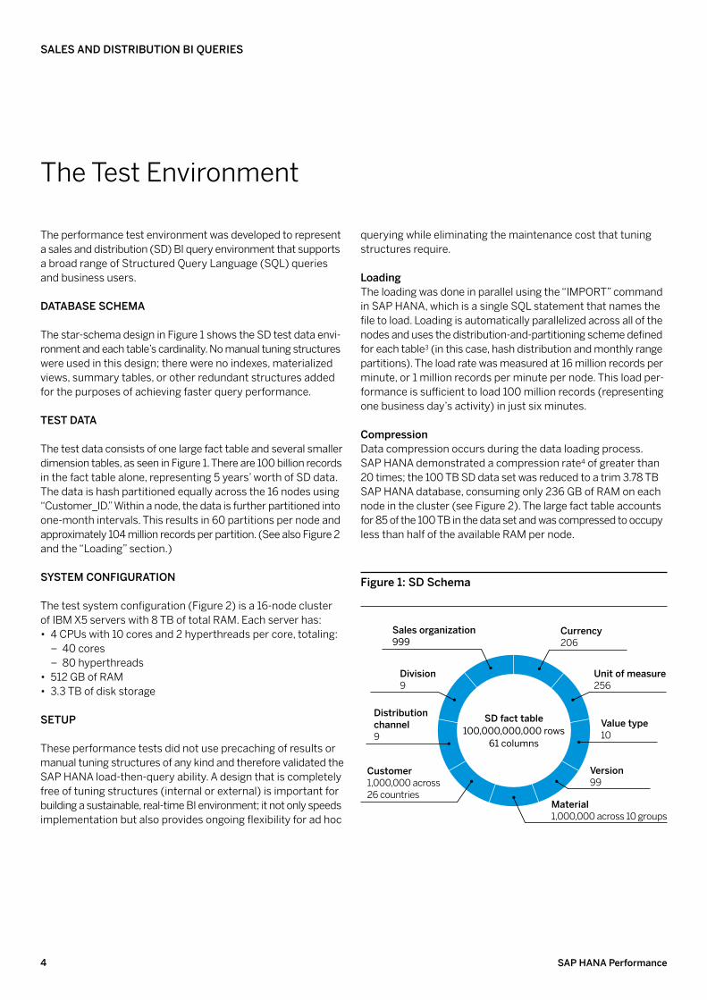
The star-schema design in Figure 1 shows the SD test data envi-ronment and each table’s cardinality. No manual tuning structures were used in this design; there were no indexes, materialized views, summary tables, or other redundant structures added for the purposes of achieving faster query performance.
TeST DATA
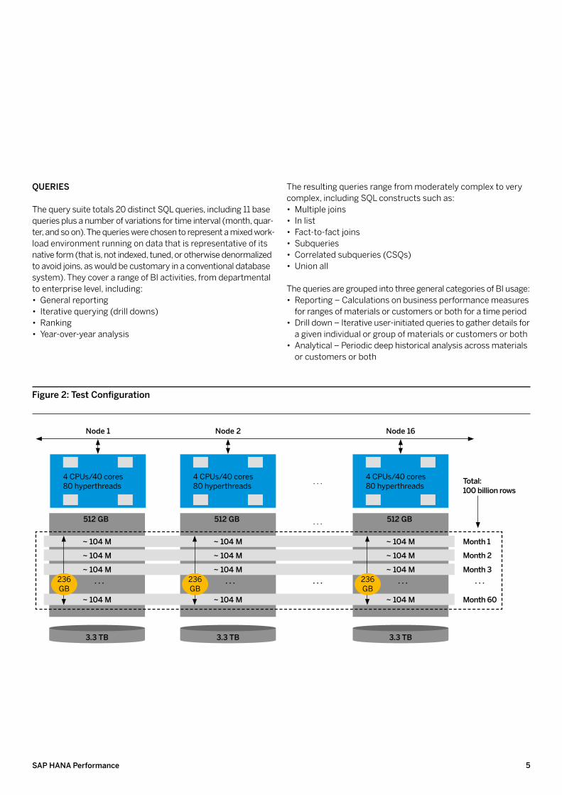
The test data consists of one large fact table and several smaller dimension tables, as seen in Figure 1. There are 100 billion records in the fact table alone, representing 5 years’ worth of SD data. The data is hash partitioned equally across the 16 nodes using “Customer_ID.” Within a node, the data is further partitioned into one-month intervals. This results in 60 partitions per node and approximately 104 million records per partition. (See also Figure 2 and the “Loading” section.)
SySTem coNfIgurATIoN
The test system configuration (Figure 2) is a 16-node cluster of IBM X5 servers with 8 TB of total RAM. Each server has:
• 4 CPUs with 10 cores and 2 hyperthreads per core, totaling: – 40 cores – 80 hyperthreads
• 512 GB of RAM • 3.3 TB of disk storage
SeTuP
These performance tests did not use precaching of results or manual tuning structures of any kind and therefore validated the SAP HANA load-then-query ability. A design that is completely free of tuning structures (internal or external) is important for building a sustainable, real-time BI environment; it not only speeds implementation but also provides ongoing flexibility for ad hoc
querying while eliminating the maintenance cost that tuning structures require.
loadingThe loading was done in parallel using the “IMPORT” command in SAP HANA, which is a single SQL statement that names the file to load. Loading is automatically parallelized across all of the nodes and uses the distribution-and-partitioning scheme defined for each table3 (in this case, hash distribution and monthly range partitions). The load rate was measured at 16 million records per minute, or 1 million records per minute per node. This load per-formance is sufficient to load 100 million records (representing one business day’s activity) in just six minutes.
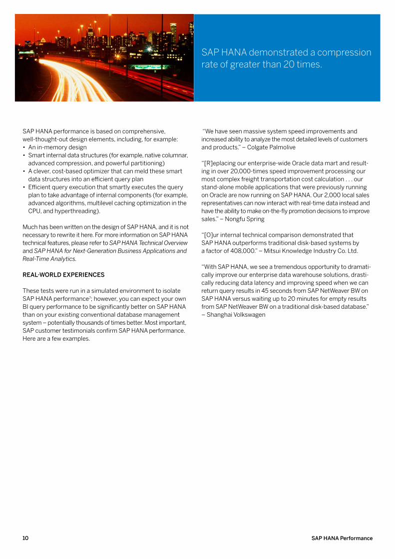
compressionData compression occurs during the data loading process. SAP HANA demonstrated a compression rate4 of greater than 20 times; the 100 TB SD data set was reduced to a trim 3.78 TB SAP HANA database, consuming only 236 GB of RAM on each node in the cluster (see Figure 2). The large fact table accounts for 85 of the 100 TB in the data set and was compressed to occupy less than half of the available RAM per node.
SAleS AND DISTrIbuTIoN bI QuerIeS
figure 1: SD Schema
currency 206
material 1,000,000 across 10 groups
customer 1,000,000 across 26 countries
Value type 10
Division 9
unit of measure 256
Sales organization 999
Version 99
Distribution channel 9
SD fact table 100,000,000,000 rows
61 columns
5SAP HANA Performance
QuerIeS
The query suite totals 20 distinct SQL queries, including 11 base queries plus a number of variations for time interval (month, quar-ter, and so on). The queries were chosen to represent a mixed work-load environment running on data that is representative of its native form (that is, not indexed, tuned, or otherwise denormalized to avoid joins, as would be customary in a conventional database system). They cover a range of BI activities, from departmental to enterprise level, including:
• General reporting • Iterative querying (drill downs) • Ranking • Year-over-year analysis
The resulting queries range from moderately complex to very complex, including SQL constructs such as:
• Multiple joins • In list • Fact-to-fact joins • Subqueries • Correlated subqueries (CSQs) • Union all
The queries are grouped into three general categories of BI usage: • Reporting – Calculations on business performance measures
for ranges of materials or customers or both for a time period • Drill down – Iterative user-initiated queries to gather details for
a given individual or group of materials or customers or both • Analytical – Periodic deep historical analysis across materials
or customers or both
Figure 2: Test Configuration
Node 16Node 2Node 1
4 CPUs/40 cores80 hyperthreads
4 CPUs/40 cores80 hyperthreads
4 CPUs/40 cores80 hyperthreads
512 gb512 gb512 gb
3.3 Tb3.3 Tb3.3 Tb
month 1
Total:100 billion rows
month 2
month 3
month 60
. . .
. . .~ 104 m~ 104 m~ 104 m
~ 104 m~ 104 m~ 104 m
~ 104 m~ 104 m~ 104 m. . .. . . . . .
. . .
. . .
. . .
~ 104 m~ 104 m~ 104 m
236 GB
236 GB
236 GB
SAP HANA Performance6
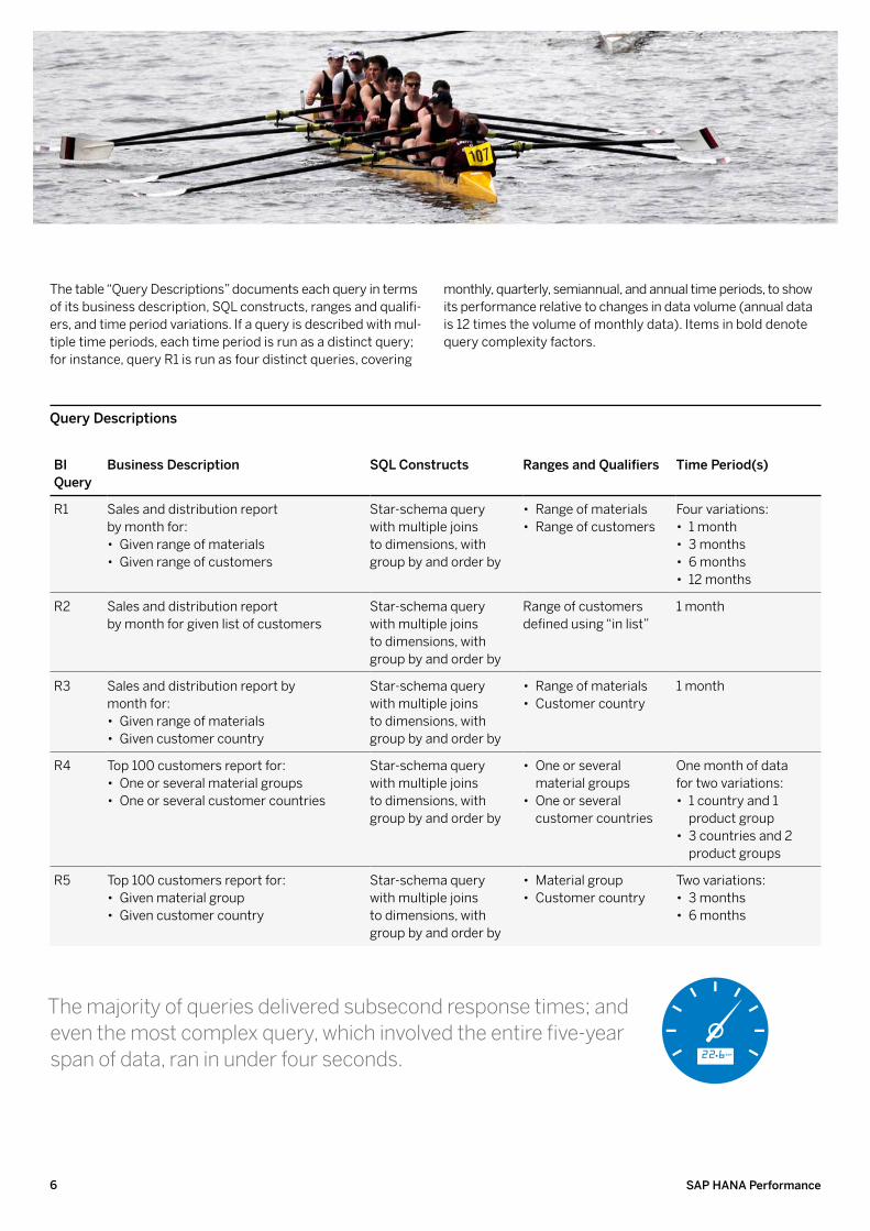
The table “Query Descriptions” documents each query in terms of its business description, SQL constructs, ranges and qualifi-ers, and time period variations. If a query is described with mul-tiple time periods, each time period is run as a distinct query; for instance, query R1 is run as four distinct queries, covering
monthly, quarterly, semiannual, and annual time periods, to show its performance relative to changes in data volume (annual data is 12 times the volume of monthly data). Items in bold denote query complexity factors.
Query Descriptions
bI Query
business Description SQl constructs Ranges and Qualifiers Time Period(s)
R1 Sales and distribution report by month for:
• Given range of materials • Given range of customers
Star-schema query with multiple joins to dimensions, with group by and order by
• Range of materials • Range of customers
Four variations: • 1 month • 3 months • 6 months • 12 months
R2 Sales and distribution report by month for given list of customers
Star-schema query with multiple joins to dimensions, with group by and order by
Range of customers defined using “in list”
1 month
R3 Sales and distribution report by month for:
• Given range of materials • Given customer country
Star-schema query with multiple joins to dimensions, with group by and order by
• Range of materials • Customer country
1 month
R4 Top 100 customers report for: • One or several material groups • One or several customer countries
Star-schema query with multiple joins to dimensions, with group by and order by
• One or several material groups
• One or several customer countries
One month of data for two variations:
• 1 country and 1 product group
• 3 countries and 2 product groups
R5 Top 100 customers report for: • Given material group • Given customer country
Star-schema query with multiple joins to dimensions, with group by and order by
• Material group • Customer country
Two variations: • 3 months • 6 months
The majority of queries delivered subsecond response times; and even the most complex query, which involved the entire five-year span of data, ran in under four seconds.
7SAP HANA Performance
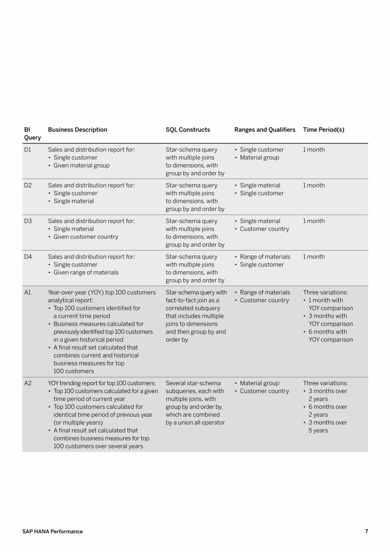
bI Query
business Description SQl constructs Ranges and Qualifiers Time Period(s)
D1 Sales and distribution report for: • Single customer • Given material group
Star-schema query with multiple joins to dimensions, with group by and order by
• Single customer • Material group
1 month
D2 Sales and distribution report for: • Single customer • Single material
Star-schema query with multiple joins to dimensions, with group by and order by
• Single material • Single customer
1 month
D3 Sales and distribution report for: • Single material • Given customer country
Star-schema query with multiple joins to dimensions, with group by and order by
• Single material • Customer country
1 month
D4 Sales and distribution report for: • Single customer • Given range of materials
Star-schema query with multiple joins to dimensions, with group by and order by
• Range of materials • Single customer
1 month
A1 Year-over-year (YOY) top 100 customers analytical report:
• Top 100 customers identified for a current time period
• Business measures calculated for previously identified top 100 customers in a given historical period
• A final result set calculated that combines current and historical business measures for top 100 customers
Star-schema query with fact-to-fact join as a correlated subquery that includes multiple joins to dimensions and then group by and order by
• Range of materials • Customer country
Three variations: • 1 month with
YOY comparison • 3 months with
YOY comparison • 6 months with
YOY comparison
A2 YOY trending report for top 100 customers: • Top 100 customers calculated for a given
time period of current year • Top 100 customers calculated for
identical time period of previous year (or multiple years)
• A final result set calculated that combines business measures for top 100 customers over several years
Several star-schema subqueries, each with multiple joins, with group by and order by, which are combined by a union all operator
• Material group • Customer country
Three variations: • 3 months over
2 years • 6 months over
2 years • 3 months over
5 years
SAP HANA Performance8
Test Results
SAleS AND DISTrIbuTIoN bI QuerIeS
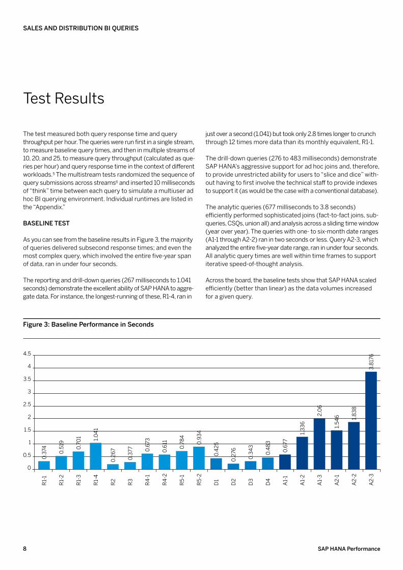
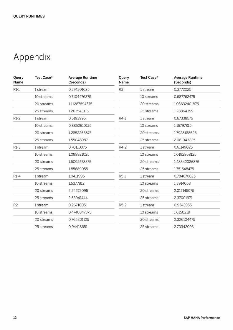
The test measured both query response time and query throughput per hour. The queries were run first in a single stream, to measure baseline query times, and then in multiple streams of 10, 20, and 25, to measure query throughput (calculated as que-ries per hour) and query response time in the context of different workloads.5 The multistream tests randomized the sequence of query submissions across streams6 and inserted 10 milliseconds of “think” time between each query to simulate a multiuser ad hoc BI querying environment. Individual runtimes are listed in the “Appendix.”
bASelINe TeST
As you can see from the baseline results in Figure 3, the majority of queries delivered subsecond response times; and even the most complex query, which involved the entire five-year span of data, ran in under four seconds.
The reporting and drill-down queries (267 milliseconds to 1.041 seconds) demonstrate the excellent ability of SAP HANA to aggre-gate data. For instance, the longest-running of these, R1-4, ran in
just over a second (1.041) but took only 2.8 times longer to crunch through 12 times more data than its monthly equivalent, R1-1.
The drill-down queries (276 to 483 milliseconds) demonstrate SAP HANA’s aggressive support for ad hoc joins and, therefore, to provide unrestricted ability for users to “slice and dice” with-out having to first involve the technical staff to provide indexes to support it (as would be the case with a conventional database).
The analytic queries (677 milliseconds to 3.8 seconds) efficiently performed sophisticated joins (fact-to-fact joins, sub-queries, CSQs, union all) and analysis across a sliding time window (year over year). The queries with one- to six-month date ranges (A1-1 through A2-2) ran in two seconds or less. Query A2-3, which analyzed the entire five-year date range, ran in under four seconds. All analytic query times are well within time frames to support iterative speed-of-thought analysis.
Across the board, the baseline tests show that SAP HANA scaled efficiently (better than linear) as the data volumes increased for a given query.
figure 3: baseline Performance in Seconds
R1-
20.
519
R1-
30.
701
R1-
41.
041
R4-
10.
673
R4-
20.
611
R5-
10.
784
R5-
20.
934
D2
0.27
6
D1
0.42
5
D3
0.34
3
D4
0.48
3
A1-
10.
677
A1-
21.
336
A1-
32.
06
A2-
11.
546
A2-
21.
838
A2-
33.
8176
R2
0.26
7
R3
0.37
7
R1-
10.
374
0
0.5
1.5
1
2
2.5
3
3.5
4
4.5
9SAP HANA Performance
THrougHPuT
The throughput tests are summarized in the table “Throughput Tests” and show that, in the face of increasing and mixed BI workloads, SAP HANA scales very well.
AD Hoc HISTorIcAl QuerIeS
The performance tests were intended primarily to demonstrate SAP HANA performance in customary real-time BI query envi-ronments that focus on analyzing business operations. However, ad hoc historical queries that analyze the entire volume of data that is stored may occasionally need to be run (and they should not impose a severe penalty). In addition to query A2-3 (included in the stream tests), queries R1-1, R4-2, and R5-1 were deemed potentially relevant for a five-year time window and were resub-mitted, this time for the entire five-year date range. The table “Ad Hoc Historical Queries” shows that SAP HANA demonstrated better-than-linear scalability running against five times more data with a response time that was three times faster or more.
Overall, these queries all ran in a few seconds and further high-light the ability of SAP HANA to support real-time BI on massive amounts of data without tuning and without massive hardware or proprietary hardware components.
reSulTS SummAry
In these performance tests, SAP HANA demonstrated the ability to deliver real-time BI-query performance as workloads increased in terms of capacity (up to 100 TB of raw data), complexity (que-ries with complex join constructs and significant intermediate results run in less than two seconds), and concurrency (25-stream throughput representing about 2,600 active users).
Test case Throughput (Queries per Hour)
1 stream 6,282
10 streams 36,600
20 streams 48,770
25 streams 52,212
Throughput Tests
At 25 streams, the average query response time was less than three seconds and is only 2.9 times higher than at baseline (see the “Appendix”), an indicator of SAP HANA’s excellent internal effi-ciencies and ability to manage concurrency and mixed workloads.
A rough estimate of BI user concurrency can be derived by divid-ing total queries per hour by an estimated average number of queries per user per hour. For instance, the 52,212 queries from the 25 streams per hour divided by 20 (a zesty per-user rate of one query every three minutes) provides a reasonable estimate of 2,610 concurrent BI users across a mixture of reporting, drill-down, and analytic query types.
Time Period r1-1 (in Seconds) r4-2 (in Seconds) r5-1 (in Seconds)
1 year 1.1 1.4 1.1
2 years 1.8 2.4 1.8
3 years 2.6 3.4 2.4
4 years 3.3 4.4 3.0
5 years 4.1 5.4 3.6
Ad Hoc Historical Queries
SAP HANA Performance10
SAP HANA performance is based on comprehensive, well-thought-out design elements, including, for example:
• An in-memory design • Smart internal data structures (for example, native columnar,
advanced compression, and powerful partitioning) • A clever, cost-based optimizer that can meld these smart
data structures into an efficient query plan • Efficient query execution that smartly executes the query
plan to take advantage of internal components (for example, advanced algorithms, multilevel caching optimization in the CPU, and hyperthreading).
Much has been written on the design of SAP HANA, and it is not necessary to rewrite it here. For more information on SAP HANA technical features, please refer to SAP HANA Technical Overview and SAP HANA for Next-Generation Business Applications and Real-Time Analytics.
reAl-WorlD exPerIeNceS
These tests were run in a simulated environment to isolate SAP HANA performance7; however, you can expect your own BI query performance to be significantly better on SAP HANA than on your existing conventional database management system – potentially thousands of times better. Most important, SAP customer testimonials confirm SAP HANA performance. Here are a few examples.
“We have seen massive system speed improvements and increased ability to analyze the most detailed levels of customers and products.” – Colgate Palmolive
“[R]eplacing our enterprise-wide Oracle data mart and result-ing in over 20,000-times speed improvement processing our most complex freight transportation cost calculation . . . our stand-alone mobile applications that were previously running on Oracle are now running on SAP HANA. Our 2,000 local sales representatives can now interact with real-time data instead and have the ability to make on-the-fly promotion decisions to improve sales.” – Nongfu Spring
“[O]ur internal technical comparison demonstrated that SAP HANA outperforms traditional disk-based systems by a factor of 408,000.” – Mitsui Knowledge Industry Co. Ltd.
“With SAP HANA, we see a tremendous opportunity to dramati-cally improve our enterprise data warehouse solutions, drasti-cally reducing data latency and improving speed when we can return query results in 45 seconds from SAP NetWeaver BW on SAP HANA versus waiting up to 20 minutes for empty results from SAP NetWeaver BW on a traditional disk-based database.” – Shanghai Volkswagen
SAP HANA demonstrated a compression rate of greater than 20 times.
11SAP HANA Performance
Real-time BI query environments should be able to support new queries as soon as users formulate them. This speed-of-thought capability is only possible if consistently excellent performance is freely available in the underlying database platform.
These rigorous performance tests and their results presented here confirm that, without tuning and without massive hard-ware or proprietary hardware components, SAP HANA delivers leading performance and scale-out ability and enables real-time BI for businesses that must support a range of analytic workloads, massive volumes of data, and thousands of concurrent users.
Conclusion
reAl-TIme bI for buSINeSSeS
SAP HANA delivers leading performance and scale-out ability and enables real-time BI for busi-nesses that must support a range of analytic work-loads, massive volumes of data, and thousands of concurrent users.
footNoteS
1. 100 TB = raw data set size before compression2. These tests did not involve SAP NetWeaver BW.3. As defined with the “CREATE TABLE” command4. Compression rates depend heavily on characteristics of the actual data being compressed. Individual results may vary.5. A single query stream represents an application connection that supports potentially hundreds of concurrent users.6. This is done to prevent a query from being submitted by different streams at exactly the same time and to help ensure a practical workload mix (for example, drill downs happen more frequently than quarterly reports).7. These performance tests were designed to isolate SAP HANA system-level performance independent of the variety of applications that may be used in SAP software environments. Therefore, these test results should be used only as a general guideline, and results will vary from implementation to implementation due to variability of platforms, applications, and data.
SAP HANA Performance12
Appendix
Query ruNTImeS
Query Name
Test case* Average runtime (Seconds)
R1-1 1 stream 0.374301625
10 streams 0.7104476375
20 streams 1.11287894375
25 streams 1.263543115
R1-2 1 stream 0.5193995
10 streams 0.8852610125
20 streams 1.2852265875
25 streams 1.55048987
R1-3 1 stream 0.70110375
10 streams 1.098921025
20 streams 1.6092578375
25 streams 1.85689055
R1-4 1 stream 1.0411995
10 streams 1.5377812
20 streams 2.24272095
25 streams 2.53941444
R2 1 stream 0.2671005
10 streams 0.4740847375
20 streams 0.765801125
25 streams 0.94418651
Query Name
Test case* Average runtime (Seconds)
R3 1 stream 0.3772025
10 streams 0.687762475
20 streams 1.03632401875
25 streams 1.28864399
R4-1 1 stream 0.67338575
10 streams 1.15797815
20 streams 1.7928188625
25 streams 2.081943225
R4-2 1 stream 0.61149025
10 streams 1.0192868125
20 streams 1.48342026875
25 streams 1.751548475
R5-1 1 stream 0.784670625
10 streams 1.3914058
20 streams 2.017145075
25 streams 2.37001971
R5-2 1 stream 0.9343955
10 streams 1.6150219
20 streams 2.326104475
25 streams 2.70342093
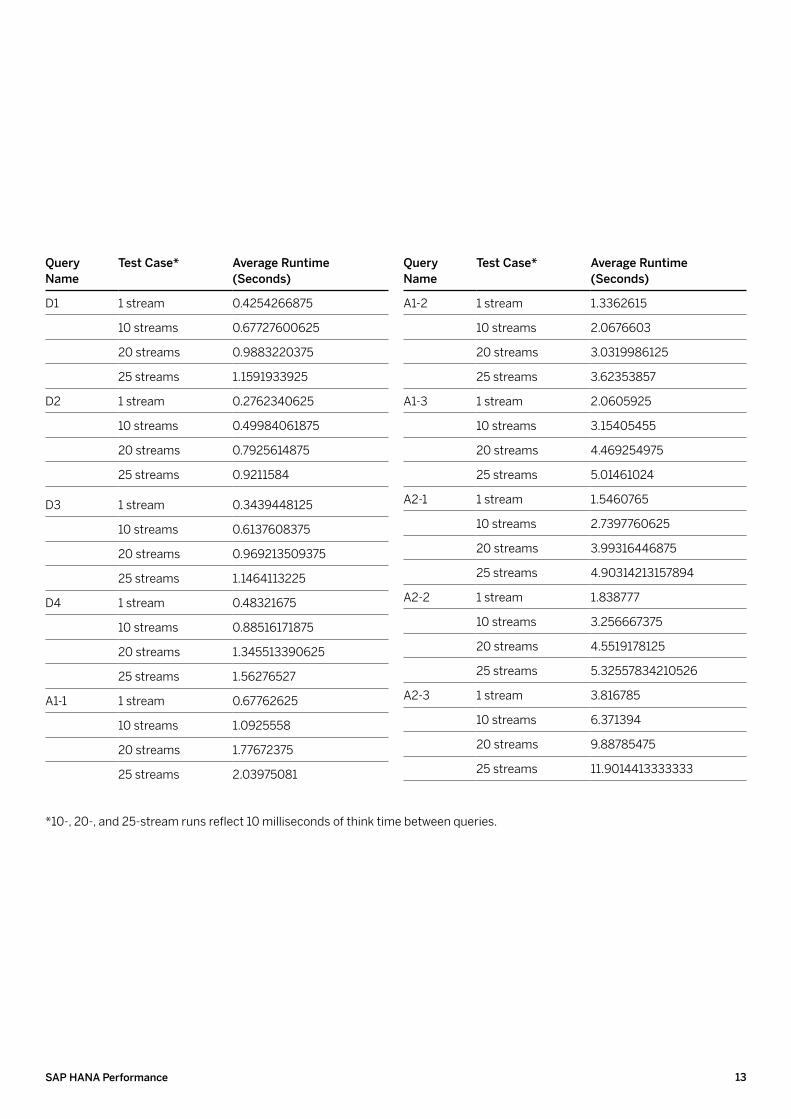
13SAP HANA Performance
Query Name
Test case* Average runtime (Seconds)
D1 1 stream 0.4254266875
10 streams 0.67727600625
20 streams 0.9883220375
25 streams 1.1591933925
D2 1 stream 0.2762340625
10 streams 0.49984061875
20 streams 0.7925614875
25 streams 0.9211584
D3 1 stream 0.3439448125
10 streams 0.6137608375
20 streams 0.969213509375
25 streams 1.1464113225
D4 1 stream 0.48321675
10 streams 0.88516171875
20 streams 1.345513390625
25 streams 1.56276527
A1-1 1 stream 0.67762625
10 streams 1.0925558
20 streams 1.77672375
25 streams 2.03975081
*10-, 20-, and 25-stream runs reflect 10 milliseconds of think time between queries.
Query Name
Test case* Average runtime (Seconds)
A1-2 1 stream 1.3362615
10 streams 2.0676603
20 streams 3.0319986125
25 streams 3.62353857
A1-3 1 stream 2.0605925
10 streams 3.15405455
20 streams 4.469254975
25 streams 5.01461024
A2-1 1 stream 1.5460765
10 streams 2.7397760625
20 streams 3.99316446875
25 streams 4.90314213157894
A2-2 1 stream 1.838777
10 streams 3.256667375
20 streams 4.5519178125
25 streams 5.32557834210526
A2-3 1 stream 3.816785
10 streams 6.371394
20 streams 9.88785475
25 streams 11.9014413333333
www.sap.com/contactsap
cmP21006 (12/07) ©2012 SAP AG. All rights reserved.
SAP, R/3, SAP NetWeaver, Duet, PartnerEdge, ByDesign, SAP BusinessObjects Explorer, StreamWork, SAP HANA, and other SAP products and services mentioned herein as well as their respective logos are trademarks or registered trademarks of SAP AG in Germany and other countries.
Business Objects and the Business Objects logo, BusinessObjects, Crystal Reports, Crystal Decisions, Web Intelligence, Xcelsius, and other Business Objects products and services mentioned herein as well as their respective logos are trademarks or registered trademarks of Business Objects Software Ltd. Business Objects is an SAP company.
Sybase and Adaptive Server, iAnywhere, Sybase 365, SQL Anywhere, and other Sybase products and services mentioned herein as well as their respective logos are trademarks or registered trademarks of Sybase Inc. Sybase is an SAP company.
Crossgate, m@gic EDDY, B2B 360°, and B2B 360° Services are registered trademarks of Crossgate AG in Germany and other countries. Crossgate is an SAP company.
All other product and service names mentioned are the trademarks of their respective companies. Data contained in this document serves informational purposes only. National product specifications may vary.
These materials are subject to change without notice. These materials are provided by SAP AG and its affiliated companies (“SAP Group”) for informational purposes only, without representation or warranty of any kind, and SAP Group shall not be liable for errors or omissions with respect to the materials. The only warranties for SAP Group products and services are those that are set forth in the express warranty statements accompanying such products and services, if any. Nothing herein should be construed as constituting an additional warranty.