Santa Ana Winds of Southern California: Their climatology,extremes, and behavior spanning six and a half decadesJanin Guzman-Morales1, Alexander Gershunov1, Jurgen Theiss2, Haiqin Li3,4, and Daniel Cayan1,5

1Scripps Institution of Oceanography, University of California, San Diego, La Jolla, California, USA, 2Theiss Research, La Jolla,California, USA, 3Cooperative Institute for Research in Environmental Science, University of Colorado Boulder, Boulder,Colorado, USA, 4Earth System Research Laboratory, National Oceanic and Atmospheric Administration, Boulder, Colorado,USA, 5United States Geological Survey, La Jolla, California, USA

Abstract Santa Ana Winds (SAWs) are an integral feature of the regional climate of Southern California/Northern Baja California region, but their climate-scale behavior is poorly understood. In the present work,we identify SAWs in mesoscale dynamical downscaling of a global reanalysis from 1948 to 2012. Model windsare validated with anemometer observations. SAWs exhibit an organized pattern with strongest easterlywinds on westward facing downwind slopes and muted magnitudes at sea and over desert lowlands. Weconstruct hourly local and regional SAW indices and analyze elements of their behavior on daily, annual, andmultidecadal timescales. SAWs occurrences peak in winter, but some of the strongest winds have occurred infall. Finally, we observe that SAW intensity is influenced by prominent large-scale low-frequency modes ofclimate variability rooted in the tropical and north Pacific ocean-atmosphere system.

1. Introduction

SAWs are episodic pulses of easterly, downslope, offshore flows over the coastal topography of theCalifornia Border Region (CBR): Southern California and Northern Baja California. SAWs represent a distinctand common regional cool season weather regime, a reversal of the typical wintertime onshore winds, con-trasted with northwesterly alongshore and onshore flow characteristic of summer [Conil and Hall, 2006].SAWs are associated with very dry air, often with anomalous warming at low elevations, and producestrong gusty downslope winds concentrated in gaps and on the lee slopes of the coastal ranges, e.g.,Santa Ana, Santa Monica, and Laguna Mountains.

It is in these rugged hills and canyons, after long dry summers characteristic of this Mediterranean climate,that SAWs can drive catastrophic wildfires that CBR is infamous for [Boyle, 1995; Moritz et al., 2010; Westerlinget al., 2004]. SAWs fanned the October 2007 wildfires that killed nine people, injured 85 others including 61 firefighters, and destroyed upward of 1500 homes, scorching 2000 km2 of land on the U.S. side of the border alone.The October 2003 SAW-fanned wildfires were even more extensive. Wind-blown smoke inhalation from these2003 wildfires in Southern California resulted in 69 premature deaths, 778 hospitalizations, 1431 emergency roomvisits, and 47K outpatient visits [Delfino et al., 2009]. More recently, the rareMay 2014 events fanned extraordinarilylate season fires following an extremely dry winter. Moreover, early and late season SAWs drive coastal heatwaves, one reason why early fall rather than summer is historically the season for the hottest temperatureextremes along the coast [Gershunov and Guirguis, 2012]. In spite of their tremendous episodic impacts onthe health, economy, andmood of the region, a direct wind-based, long-term, and high-frequency climatologyof SAWs is not available and relationships with larger-scale climate variability have not been clearly elucidated.This article begins to address these knowledge gaps for SAW behavior.

Indirect or proxy-based climatologies of SAWs have been typically diagnosed from synoptic-scale information.Raphael [2003] diagnosed 33 years of daily SAWs from observed pressure fields, while Jones et al. [2010]diagnosed 28 years of daily Fire Weather Index (FWI) [Fosberg, 1978] values, of which dry winds are acomponent, derived from the North American Regional Reanalysis [Mesinger et al., 2006]. Abatzoglou et al.[2013] developed the longest empirical daily reconstruction to date, from 1948 to 2012 based on pressure fieldsand temperature advection from global reanalysis.

Mesoscale modeling (MSM) has also been employed in the study of SAWs, typically to investigate the anatomyof SAWs from small samples of individual events [e.g., Sommers, 1978; Lu et al., 2012]. Moritz et al. [2010]provided a longer perspective using a decade of SAWs dynamically downscaled and demonstrated the ability

GUZMAN-MORALES ET AL. SANTA ANA WINDS OF SOUTHERN CALIFORNIA 1

PUBLICATIONSGeophysical Research Letters

RESEARCH LETTER10.1002/2016GL067887

Key Points:• A 65 year record of hourly Santa AnaWinds has been created

• ENSO and PDO modulate Santa AnaWinds intensity

• Santa Ana Winds increased in intensitywith the 1970s PDO shift

Supporting Information:• Supporting Information S1

Correspondence to:J. Guzman-Morales,jguzmanmorales@ucsd.edu

Citation:Guzman-Morales, J., A. Gershunov,J. Theiss, H. Li, and D. Cayan (2016),Santa Ana Winds of SouthernCalifornia: Their climatology,extremes, and behavior spanning sixand a half decades, Geophys. Res.Lett., 43, doi:10.1002/2016GL067887.

Received 27 JAN 2016Accepted 9 MAR 2016Accepted article online 14 MAR 2016

©2016. American Geophysical Union.All Rights Reserved.

to predict large observed wildfirelocations via model-derived FWI. Otherstudies have also employed MSM datasets spanning up to a decade with highspatiotemporal resolution to characterizeSAWs among Southern California’s regio-nal weather regimes [Conil and Hall, 2006]and to investigate their causal mechan-isms [Hughes and Hall, 2010]. Followingon this work, Hughes et al. [2011] investi-gated anthropogenic climate changeimpacts on SAWs.

Here we usemesoscale modeling-derivedwind data exclusively to define andquantify a long record of observationallyvalidated SAWs. In what follows, we useobserved wind to validate hourly windsin a 65 year dynamical downscaling of aglobal reanalysis to 10 km. We developand apply a SAW definition with locallyspecific wind thresholds, and after deter-mining their canonical spatial footprint,we define a SAW Domain, from whicha SAW Regional Index is constructed.Subsequently, we examine the SAW cli-

matology, paying particular attention to extremes, noteworthy events, interannual and longer-term variability.We finally discuss results in the context of regional climate variability, predictability and change, and in termsof their relevance to wildfire.

2. Data and Methods2.1. Modeled Winds

To examine SAW variability in space and time, we use winds from the California Reanalysis Downscaling to10 km, CaRD10 [Kanamitsu and Kanamaru, 2007]. CaRD10 provides hourly instantaneous winds at 10m abovethe ground from 1948 to 2012, which is the longest mesoscale record to date. Our domain extends from(118.115°W, 35.081°N) at the NW point to (116.035°W, 32.053°N) at the most SE point with a total of 756 gridcells (21× 36), capturing the core of the CBR extending 65 km across the border into Northern Baja California,Mexico (Figure 1).

2.2. Validation

Themodel skill is tested against sustainedwind (wind speed average) andwind gust (maximum “instantaneous”wind speed) observations from 85 Remote Automated Weather Stations (RAWS) and one Automated SurfaceObserving System station (ASOS) across the domain (shown in Figure 1). Correlation coefficient (r) andnormalized root mean squared error (NRMSE) are calculated for the overlapping part of the stations andCaRD10 records.

CaRD10 winds correlate more strongly with gusts than sustained winds at 78 (91% of) stations. This consistentlystronger link with observed gusts is seen on the histograms shown in Figures S1a and S1b. Errors, measured asNRMSE, against gusts are also consistently smaller than errors against sustainedwinds (Figures S2a and S2b); thisis the case at 65 (76% of) stations. When using SAWs (see section 2.3 for the definition of SAW) only, correlationsat some stations improve but deteriorate at others (see flatter histograms in Figures S1c and S1d compared toFigures S1a and S1b). However, the agreement between modeled SAWs and observations still consistentlyfavors observed gust over sustained wind (Figures S1c, S1d, S2c, and S2d). Modeled winds are instantaneous,neither sustained nor gust. Modeled winds overestimate sustained near-surface winds. Beyond possible modelbiases, part of the reason for this may be that observed winds are affected by fine-scale orography, as well as

Figure 1. Spatial domain of the CBR with topography. Elevation is shownat 60 arc sec (colors) and 10 km spatial resolution (contours). Black dotsmark the location of RAWS, and yellow dots show ASOS at RamonaAirport labeled “R.” Location of Witch Creek Fire (WF) start in late October2007 is shown as a red dot.

Geophysical Research Letters 10.1002/2016GL067887

GUZMAN-MORALES ET AL. SANTA ANA WINDS OF SOUTHERN CALIFORNIA 2

obstructions around the anemometer, not resolved by the model. Gusts are less sensitive to such features asthey are more related to the flow above the boundary layer via turbulent mixing [Brasseur, 2001].

2.3. Local Definition of Santa Ana Winds

Modeled strong winds tend to converge between easterly and northeasterly directions with surface relativehumidity dropping into single digits (Figure S3). This behavior suggests that wind direction and speed aresufficient to define SAWs. At each grid cell or station, we first identify winds with directions > 0° and< 180° (winds with a negative u component) and define local speed thresholds as the upper quartile ofthe direction-selected winds. Periods with at least 12 h of continuous selected winds that exceed the localwind speed threshold for at least 1 h are defined as SAWs. Discontinuities are allowed for periods of 12 hor less, to allow for breaks in SAW events, e.g., competing afternoon sea breeze episodes. The resultingSAW index reflects the full wind speed during periods that fulfill the direction-continuity scheme.

Ramona, California (Figure 1), located in west facing foothills of the Laguna Mountains, is known to be awindy fire prone location where the late October Cedar Fire (2003) andWitch Creek Fire (2007) burned duringsevere multiple wildfire episodes. In this work, we turn to Ramona for local examples. The correlation for thewhole period of available gust and sustained wind observations (from 2005 to 2010) with Ramona SAW is 0.7and 0.6, respectively. Figure S4b shows the excellent agreement between SAW and observed gust at Ramona,during early season SAW events of 2007 and 2010.

2.4. Regionalizing Local SAWs

We examine the spatial and seasonal coherence of locally defined SAWs. In the CaRD10 data set, the strongestSAWs are found on downwind slopes of the main topography, while SAWs relative to other winds reflect analmost identical pattern (Figures 2a and 2b) with comparatively lower values at sea, and lowest values over

Figure 2. SAW spatial patterns. (a) Means, (b) ratios of SAW to all other winds, (c) correlations of local SAW time series withthe leading SAW principal component (PC1), and (d) correlations of SAWRI time series with Ramona SAW. Black line marksSAW Domain on each map. All means and correlations are based on hourly data.

Geophysical Research Letters 10.1002/2016GL067887

GUZMAN-MORALES ET AL. SANTA ANA WINDS OF SOUTHERN CALIFORNIA 3

the desert basins. This SAW speed spatial distribution is notably consistent with Hughes and Hall [2010]who determined it to be forced by katabatic acceleration of cool air downslope as well as downwardmomentum transfer.

We calculate the empirical orthogonal functions of hourly SAWs. The leading principal component (PC1)explains 50% of the total hourly SAWs variance over the region and its time series corresponds to SAWseasonality (Figure S5a). Broad regional coherence of SAW selection is displayed as correlations of PC1 withSAWs time series (Figure 2c). We also quantify the regional concurrence of SAWs across the domain withRamona SAWs (Figure 2d), noting that SAWs at selected locations are well represented by the regionalaggregate SAW index (described below).

Consistent with the above results, we define the SAWDomain as the region displaying coherent SAWs in timeand magnitude. Thus, the SAW Domain is explicitly constrained to grid cells where PC1 explains 50% of thevariance, i.e., where correlations between SAWs and PC1 exceed 0.7 and by high wind speed ratios (>1.5). Forthe sake of continuity, we include the low-ratio cluster of grid cells northeast of the Santa Ana Mountains andadjacent ocean grid cells (~40 km offshore). SAW Domain covers 43% of the original domain (Figure 2).

The SAW Regional Index (SAWRI) is then defined as the hourly average of the SAWs across all the grid cellswithin the SAW Domain. Hourly SAWRI is correlated with PC1 at r=0.9 and with Ramona SAWs at r=0.7.We reconstruct two seasons of observed SAW Regional Index (SAWRIobs) from in situ wind observations.The correlation between the hourly SAWRI and SAWRIobs is 0.6. Comparison at different temporal resolutionsis shown in Figure S5.

SAW events are directly quantified by continuous periods of SAWRI and classified into three categoriesaccording to their maximum SAWRI—weak (<5m s!1), moderate (5–10m s!1), and extreme (10–15m s!1).Extremes events are above the 90th percentile of all events on record. Finally, we integrate SAWRI overtimeto obtain total seasonal SAW intensity.

3. Results3.1. SAW Climatology

Regionally, i.e., using SAWRI we detect a total of 2056 events on the 65 year record yielding an average of 32occurrences per year. Typical SAW episodes last 1–2 days and represent 27% of the occurrences (Figure S6a).SAW events lasting up to 6 days account for 90% of all occurrences. The remaining 10% are made up almostentirely of events lasting between 7 and 12 days. Locally, the occurrence of events lasting 1–2 days isconsistent with regional detection (also 27% of all events). However, shorter events (between 12 and 24 h)are the most frequent (Figure S6b). This suggests that mild SAW pulses over most active SAW locations(red areas in Figure 2a) may not be detected regionally, as they dissipate before reaching the coast. Themeanand maximum SAWRI representing events lasting up to 5 days appear to increase linearly with duration(Figures S6c and S6e). For events longer than 5 days, the mean and maximum SAWRI reach limit speeds(~5 and 9m s!1, respectively) regardless of their duration. The duration-intensity relation for local SAWs iscomparable (see Figures S6d and S6f) to regional results.

The SAW season extends from October to April, when SAW events occur at least twice per average month(Figure 3d). SAWs tend to be most frequent in December but most durable and strong in January. Early andlate season SAW episodes occur, on average, about once per month in September and May, and typicallyexhibit moderate duration, and moderate regional speeds, i.e., mean and maximum SAWRI (Figures 3a–3c).Although not on our record, the two events of May 2014 (http://abcnews.go.com/topics/news/weather/santa-ana-winds.htm) appear to have been exceptional. This seasonal cycle of SAWs, although describedin more detail here, generally agrees with seasonality identified in other studies [Jones et al., 2010;Raphael, 2003].

In addition to the seasonal cycle, the hourly SAWRI resolves a well-defined diurnal cycle (Figure S7), reachingtheir maximum in the morning and decay to their minimum in the late afternoon. Local diurnal cycle of SAWsis line with SAWRI; however, inland and coastal locations are slightly different. At the coast, the onshore seabreeze may to some extent counteract SAWs starting in the morning and during some events the winds mayreverse in the late afternoon.

Geophysical Research Letters 10.1002/2016GL067887

GUZMAN-MORALES ET AL. SANTA ANA WINDS OF SOUTHERN CALIFORNIA 4

3.2. Climatology of SAW Extremes

Under the SAW and extreme definitions established, extremes account for 10% of the total number of events(on average three events per year). Extreme SAWs are most common in December, and January, but alsooccur in the shoulder seasons, with more extremes in fall compared to spring (red histogram in Figure 3d).Even though the highest frequency of extreme events is observed during the coldest months, maximumSAWRI can be just as extreme in the fall (Figure 3b). For example, three out of the top five SAW events withmaximum SAWRI above 15m s!1 occurred in fall.

3.3. Variability and Trends

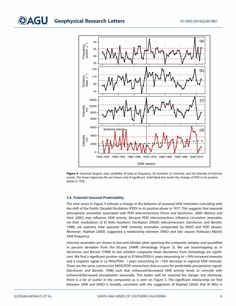
Our results indicate considerable variability of SAW frequency, duration, and total intensity (total or by cate-gory) on interannual to decadal time scales. There are no significant long-term trends (Figures 4a–4c), exceptfor a modest upward trend in the intensity of extreme SAWs (Figure 4d). For the record the frequency ofextreme events accounts for 9% of all SAW events, but they contribute 25% to the total seasonal intensity.Closer examination reveals that this trend results mainly from a step-function-type change that roughly cor-responds to the North Pacific climate shift in the mid-1970s [Mantua and Hare, 2002]. A similar shift is alsoevident in the SAW duration and intensity (Figures 4b and 4c). The shift in these other variables, althoughnot resulting in a significant trend, is much more in line with the 1976 Pacific Decadal Oscillation (PDO) shift.

Figure 3. Climatology of regional SAW events (SAWRI). Monthly distribution of (a) mean SAWRI per event, (b) maximumSAWRI per event, (c) duration, and (d) mean monthly frequency per season of SAW events detected from 1948 to 2012.In Figures 3a–3c bold lines show median values, boxes delimit the first and third quartiles, and whiskers mark maximumand minimum values for each month. Extremes SAWs are shown in dark red in Figures 3b and 3d.

Geophysical Research Letters 10.1002/2016GL067887

GUZMAN-MORALES ET AL. SANTA ANA WINDS OF SOUTHERN CALIFORNIA 5

3.4. Potential Seasonal Predictability

The time series in Figure 4 indicate a change in the behavior of seasonal SAW intensities coinciding withthe shift of the Pacific Decadal Oscillation (PDO) to its positive phase in 1977. This suggests that seasonalatmospheric anomalies associated with PDO teleconnections [Favre and Gershunov, 2009; Mantua andHare, 2002] may influence SAW activity. Because PDO teleconnections influence circulation anomaliesvia their modulation of El Niño–Southern Oscillation (ENSO) teleconnections [Gershunov and Barnett,1998], we examine total seasonal SAW intensity anomalies composited by ENSO and PDO phases.Moreover, Raphael [2003] suggested a relationship between ENSO and late season (February–March)SAW frequency.

Intensity anomalies are shown in box-and-whisker plots spanning the composite samples and quantifiedin percent deviation from the 65 year SAWRI climatology (Figure 5). We use bootstrapping as inGershunov and Barnett [1998] to test whether composite mean deviations from climatology are signifi-cant. We find a significant positive signal in El Niño/PDO(+) years amounting to ~10% increased intensityand a negative signal in La Niña/PDO(!) years amounting to ~10% decrease in regional SAW intensity.These are the same constructive ENSO/PDO interactions that account for predictable precipitation signals[Gershunov and Barnett, 1998] such that enhanced/decreased SAW activity tends to coincide withenhanced/decreased precipitation seasonally. This bodes well for seasonal fire danger, but obviously,there is a lot of scatter in the composites as is seen on Figure 5. The significant relationship we findbetween SAW and ENSO is broadly consistent with the suggestion of Raphael [2003] that El Niño is

25

30

35

40

Fre

quen

cy

(a)

Dur

atio

n

70

90

110

130 (b)

6000

8000

10000

12000

Inte

nsity

(m)

(c)

0

2000

4000

6000

Inte

nsity

(m)

1948 1949 1958 1959 1968 1969 1978 1979 1988 1989 1998 1999 2009 2010

Extreme events (d)

SAW season

Figure 4. Seasonal (August–July) variability of total (a) frequency, (b) duration, (c) intensity, and (d) intensity of extremeevents. The linear regression fits are shown only if significant. Solid black line marks the change of PDO to its positivephase in 1976.

Geophysical Research Letters 10.1002/2016GL067887

GUZMAN-MORALES ET AL. SANTA ANA WINDS OF SOUTHERN CALIFORNIA 6

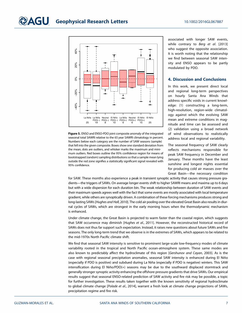
associated with longer SAW events,while contrary to Berg et al. [2013]who suggest the opposite association.It is worth noting that the relationshipwe find between seasonal SAW inten-sity and ENSO appears to be partlymodulated by PDO.

4. Discussion and Conclusions

In this work, we present direct localand regional long-term perspectiveson hourly Santa Ana Winds thataddress specific voids in current knowl-edge: (1) constructing a long-term,high-resolution, region-wide climatol-ogy against which the evolving SAWmean and extreme conditions in mag-nitude and time can be assessed and(2) validation using a broad networkof wind observations to realisticallyaddress local and regional variability.

The seasonal frequency of SAW clearlyreflects mechanisms responsible forpeak SAW frequency in December andJanuary. These months have the leastsunshine and longest nights essentialfor producing cold air masses over theGreat Basin—the necessary condition

for SAW. These months also experience a peak in transient synoptic activity that causes strong pressure gra-dients—the triggers of SAWs. On average longer events shift to higher SAWRI means and maxima up to 6daysbut with a wide dispersion for each duration bin. The weak relationship between duration of SAW events andtheir maximum speeds agrees well with the fact that some events are mostly associated with local temperaturegradient, while others are synoptically driven. A combination of these forcingmechanisms produces strong andlong-lasting SAWs [Hughes and Hall, 2010]. The cold air pooling over the elevated Great Basin also results in diur-nal cycles of SAWs, which are strongest in the early morning hours when the thermodynamic mechanismis enhanced.

Under climate change, the Great Basin is projected to warm faster than the coastal region, which suggeststhat SAW occurrence may diminish [Hughes et al., 2011]. However, the reconstructed historical record ofSAWs does not thus far support such expectation. Instead, it raises new questions about future SAWs and fireseasons. The only long-term trend that we observe is in the extremes of SAWs, which appears to be related tothe mid-1970s North Pacific climate shift.

We find that seasonal SAW intensity is sensitive to prominent large-scale low-frequency modes of climatevariability rooted in the tropical and North Pacific ocean-atmosphere system. These same modes arealso known to predictably affect the hydroclimate of this region [Gershunov and Cayan, 2003]. As is thecase with regional seasonal precipitation anomalies, seasonal SAW intensity is enhanced during El Niño(especially if PDO is positive) and subdued during La Niña (especially if PDO is negative) winters. This SAWintensification during El Niño/PDO(+) seasons may be due to the southward displaced stormtrack andgenerally stronger synoptic activity enhancing the offshore pressure gradients that drive SAWs. Our empiricalresults suggest that seasonal ENSO-related prediction of SAW activity and fire risk may be possible, a topicfor further investigation. These results taken together with the known sensitivity of regional hydroclimateto global climate change [Polade et al., 2014], warrant a fresh look at climate change projections of SAWs,precipitation regime and fire risk.

25 19 8 10 6 6 15 25

40%

20%

0%20

%40

%

Figure 5. ENSO and ENSO-PDO joint composite anomaly of the integratedseasonal total SAWRI relative to the 65 year SAWRI climatology in percent.Numbers below each category are the number of SAW seasons (sample)that fell into the given composite. Boxes show one standard deviation fromthe mean, dots are outliers, and whisker marks the maximum and mini-mum outliers. Red boxes outline the 95% confidence region for means ofbootstrapped (random) sampling distributions so that a samplemean lyingoutside the red zone signifies a statistically significant signal revealed with95% confidence.

Geophysical Research Letters 10.1002/2016GL067887

GUZMAN-MORALES ET AL. SANTA ANA WINDS OF SOUTHERN CALIFORNIA 7

ReferencesAbatzoglou, J. T., R. Barbero, and N. J. Nauslar (2013), Diagnosing Santa Ana Winds in Southern California with synoptic-scale analysis,

Weather Forecast., 28(3), 704–710.Berg, N., et al. (2013), El Niño-Southern Oscillation impacts on winter winds over Southern California, Clim. Dyn., 40(1), 109–121.Boyle, T. C. (1995), The Tortilla Curtain, 368 pp., Viking, New York.Brasseur, O. (2001), Development and application of a physical approach to estimating wind gusts, Mon. Weather Rev., 129(1), 5–25.Conil, S., and A. Hall (2006), Local regimes of atmospheric variability: A case study of Southern California, J. Clim., 19(17), 4308–4325.Delfino, R. J., et al. (2009), The relationship of respiratory and cardiovascular hospital admissions to the Southern California wildfires of 2003,

Occup. Environ. Med., 66(3), 189–197.Favre, A., and A. Gershunov (2009), North Pacific cyclonic and anticyclonic transients in a global warming context: Possible consequences for

Western North American daily precipitation and temperature extremes, Clim. Dyn., 32(7–8), 969–987.Fosberg, M. A. (1978), Weather in wildland fire management—Fire weather index, Bull. Am. Meteorol. Soc., 59(3), 341.Gershunov, A., and T. P. Barnett (1998), Interdecadal modulation of ENSO teleconnections, Bull. Am. Meteorol. Soc., 79(12), 2715–2725.Gershunov, A., and D. R. Cayan (2003), Heavy daily precipitation frequency over the contiguous United States: Sources of climatic variability

and seasonal predictability, J. Clim., 16(16), 2752–2765.Gershunov, A., and K. Guirguis (2012), California heat waves in the present and future,Geophys. Res. Lett., 39, L18710, doi:10.1029/2012GL052979.Hughes, M., and A. Hall (2010), Local and synoptic mechanisms causing Southern California’s Santa Ana Winds, Clim. Dyn., 34(6), 847–857.Hughes, M., A. Hall, and J. Kim (2011), Human-induced changes in wind, temperature and relative humidity during Santa Ana events, Clim.

Change, 109, 119–132.Jones, C., F. Fujioka, and L. M. V. Carvalho (2010), Forecast skill of synoptic conditions associated with Santa Ana Winds in Southern California,

Mon. Weather Rev., 138(12), 4528–4541.Kanamitsu, M., and H. Kanamaru (2007), Fifty-seven-year California Reanalysis Downscaling at 10 km (CaRD10). Part I: System detail and

validation with observations, J. Clim., 20(22), 5553–5571.Lu, W., S. Zhong, J. J. Charney, X. Bian, and S. Liu (2012), WRF simulation over complex terrain during a southern California wildfire event,

J. Geophys. Res., 117, D05125, doi:10.1029/2011JD017004.Mantua, N. J., and S. R. Hare (2002), The Pacific decadal oscillation, J. Oceanogr., 58(1), 35–44.Mesinger, F., et al. (2006), North American regional reanalysis, Bull. Am. Meteorol. Soc., 87(3), 343–360.Moritz, M. A., T. J. Moody, M. A. Krawchuk, M. Hughes, and A. Hall (2010), Spatial variation in extreme winds predicts large wildfire locations in

chaparral ecosystems, Geophys. Res. Lett., 37, L04801, doi:10.1029/2009GL041735.Polade, S. D., D. W. Pierce, D. R. Cayan, A. Gershunov, and M. D. Dettinger (2014), The key role of dry days in changing regional climate and

precipitation regimes, Sci. Rep., 4, 4364.Raphael, M. N. (2003), The Santa Ana Winds of California, Earth Interact., 7, 1–13, doi:10.1175/1087-3562(2003)007<0001:TSAWOC>2.0.CO;2.Sommers, W. T. (1978), LFM forecast variables related to Santa-Ana Wind occurrences, Mon. Weather Rev., 106(9), 1307–1316.Westerling, A. L., D. R. Cayan, T. J. Brown, B. L. Hall, and L. G. Riddle (2004), Climate, Santa Ana Winds and autumn wildfires in Southern

California, Eos Trans. AGU, 85(31), 289–296, doi:10.1029/2004EO310001.

Geophysical Research Letters 10.1002/2016GL067887

GUZMAN-MORALES ET AL. SANTA ANA WINDS OF SOUTHERN CALIFORNIA 8

AcknowledgmentsWe are grateful to CONACYT-UCMEXUS(http://ucmexus.ucr.edu/) for providingfinancial support to Janin Guzman-Morales(scholar 214550). We also appreciatesupport from Climate Education Partners,a National Science Foundation fundedproject DUE-1239797 (www.sandiego.edu/climate). This study also contributesto DOI’s Southwest Climate ScienceCenter activities and NOAA’s Californiaand Nevada Applications Program awardNA11OAR43101. The derived griddeddata of local SAWs as well as the SAWRIcan be accessed at http://cnap.ucsd.edu/data/janin/.