EE104 S. Lall and S. Boyd

Features

Sanjay Lall and Stephen Boyd

EE104Stanford University

1

Records and embedding

2

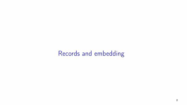
Raw data

I raw data pairs are (u; v), with u 2 U , v 2 V

I U is set of all possible input values

I V is set of all possible output values

I each u is called a record

I typically a record is a tuple, or list, u = (u1; u2; : : : ; ur)

I each ui is a field or component, which has a type, e.g., real number, Boolean, categorical, ordinal, word,text, audio, image, parse tree (more on this later)

I e.g., a record for a house for sale might consist of

(address; photo; description; house/apartment?; lot size; : : : ;# bedrooms)

3

Feature map

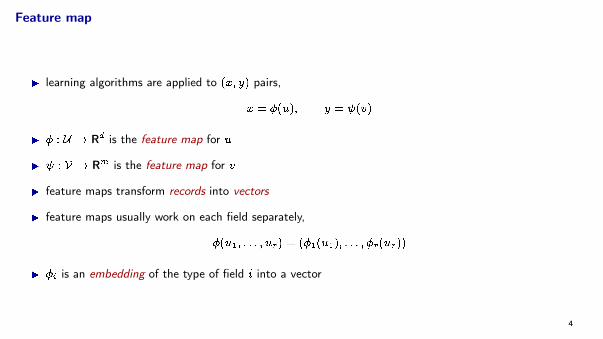
I learning algorithms are applied to (x; y) pairs,

x = �(u); y = (v)

I � : U ! Rd is the feature map for u

I : V ! Rm is the feature map for v

I feature maps transform records into vectors

I feature maps usually work on each field separately,

�(u1; : : : ; ur) = (�1(u1); : : : ; �r(ur))

I �i is an embedding of the type of field i into a vector

4

Embeddings

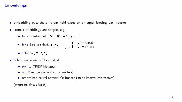
I embedding puts the different field types on an equal footing, i.e., vectors

I some embeddings are simple, e.g.,

I for a number field (U = R), �i(ui) = ui

I for a Boolean field, �i(ui) =

�1 ui = true

�1 ui = false

I color to (R;G;B)

I others are more sophisticated

I text to TFIDF histogram

I word2vec (maps words into vectors)

I pre-trained neural network for images (maps images into vectors)

(more on these later)

5

Faithful embeddings

a faithful embedding satisfies

I �(u) is near �(~u) when u and ~u are ‘similar’

I �(u) is not near �(~u) when u and ~u are ‘dissimilar’

I lefthand concept is vector distance

I righthand concept depends on field type, application

I interesting examples: names, professions, companies, countries, languages, ZIP codes, cities, songs,movies

I we will see later how such embeddings can be constructed

6

Examples

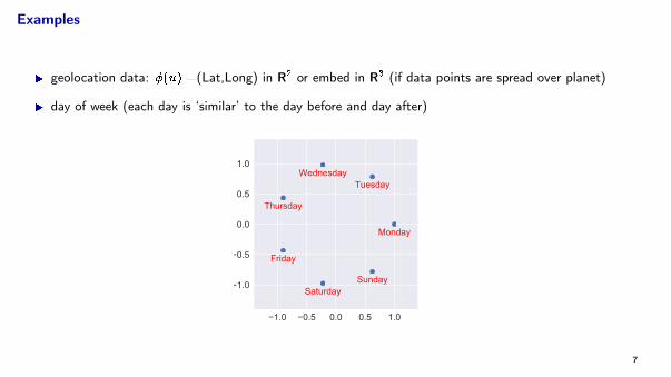
I geolocation data: �(u) =(Lat,Long) in R2 or embed in R3 (if data points are spread over planet)

I day of week (each day is ‘similar’ to the day before and day after)

1.0 0.5 0.0 0.5 1.0

1.0

0.5

0.0

0.5

1.0

Monday

TuesdayWednesday

Thursday

Friday

SaturdaySunday

7

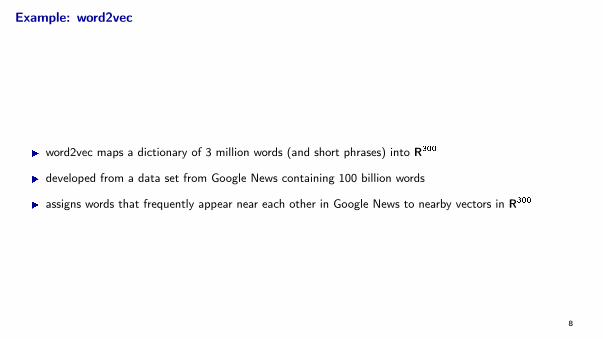
Example: word2vec

I word2vec maps a dictionary of 3 million words (and short phrases) into R300

I developed from a data set from Google News containing 100 billion words

I assigns words that frequently appear near each other in Google News to nearby vectors in R300

8

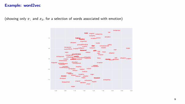
Example: word2vec

(showing only x1 and x2, for a selection of words associated with emotion)

2.25 2.00 1.75 1.50 1.25 1.00 0.75 0.50 0.25

1.0

0.5

0.0

0.5

1.0

tenderness

helpless

defeated

sympathy

outraged

content

adoration

dreading

rejected

hostile

proud

distrusting

disillusioned

bitter

satisfiedreceptive

suspicious

interested

cautious

confused

scornful

amused

disturbed

elated

shocked

overwhelmed

helpless

vengeful

enthusiastic

exhilarated

uncomfortable

isolated

disliked

optimistic

dismayed

guiltynumb

amazed

regretful

confused

lonely

ambivalent

alienated

calm

stunned

melancholy

exhausted

bitter

relaxed

interested

depressedinsulted

relieved

hopeless

disgusted

indifferent

hopeful

absorbed

curious

guilty

revulsion

anticipating

brave

eager

lonely

comfortable

hesitant

regretfulsafefearful

depressed

preoccupied

happy

anxious

hopeless

angry love

worried

sorrow

jealous

lust

scareduncertain

aroused

anguished

annoyed

tender

rejected

disappointed

compassionate

horrified

irritated

caring

alarmed

shocked

embarrassed concernpanicked

grumpy

trustawkward

liking

uncomfortableexasperated

attraction

disoriented

frustrated

9

Imagenet embedding

I Imagenet is an open image database with 14m labeled images in 1000 classes

I vgg16 maps images u (224� 224 pixels with R,G,B components) to x 2 R4096

I vgg16 was originally developed to classify the image labels

I repurposed as general image feature mapping

I vgg16 has neural network form with 16 layers, with input u, output x

10

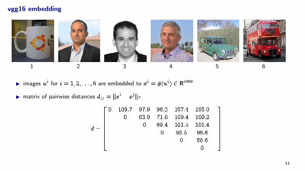
vgg16 embedding

1 2 3 4 5 6

I images ui for i = 1; 2; : : : ; 6 are embedded to xi = �(ui) 2 R4096

I matrix of pairwise distances dij = kxi � xjk2

d =

2666664

0 109:7 97:9 96:2 107:4 103:0

0 63:9 71:6 109:4 109:2

0 69:4 101:5 101:4

0 96:5 96:8

0 86:6

0

3777775

11

Standardized embeddings

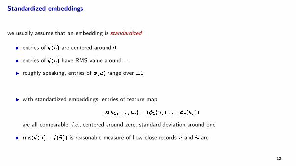
we usually assume that an embedding is standardized

I entries of �(u) are centered around 0

I entries of �(u) have RMS value around 1

I roughly speaking, entries of �(u) range over �1

I with standardized embeddings, entries of feature map

�(u1; : : : ; ur) = (�1(u1); : : : ; �r(ur))

are all comparable, i.e., centered around zero, standard deviation around one

I rms(�(u)� �(~u)) is reasonable measure of how close records u and ~u are

12

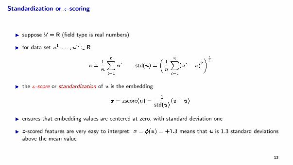
Standardization or z-scoring

I suppose U = R (field type is real numbers)

I for data set u1; : : : ; un 2 R

�u =1

n

nXi=1

ui std(u) =

�1

n

nXi=1

(ui � �u)2� 1

2

I the z-score or standardization of u is the embedding

x = zscore(u) =1

std(u)(u� �u)

I ensures that embedding values are centered at zero, with standard deviation one

I z-scored features are very easy to interpret: x = �(u) = +1:3 means that u is 1.3 standard deviationsabove the mean value

13

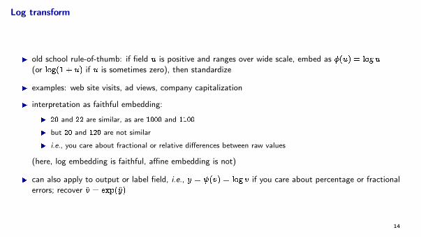
Log transform

I old school rule-of-thumb: if field u is positive and ranges over wide scale, embed as �(u) = logu

(or log(1 + u) if u is sometimes zero), then standardize

I examples: web site visits, ad views, company capitalization

I interpretation as faithful embedding:

I 20 and 22 are similar, as are 1000 and 1100

I but 20 and 120 are not similar

I i.e., you care about fractional or relative differences between raw values

(here, log embedding is faithful, affine embedding is not)

I can also apply to output or label field, i.e., y = (v) = log v if you care about percentage or fractionalerrors; recover v = exp(y)

14

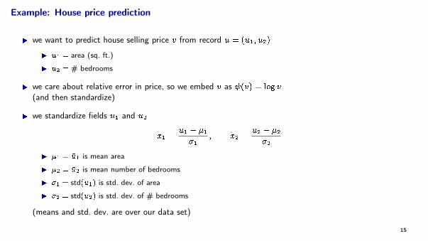
Example: House price prediction

I we want to predict house selling price v from record u = (u1; u2)

I u1 = area (sq. ft.)

I u2 = # bedrooms

I we care about relative error in price, so we embed v as (v) = log v

(and then standardize)

I we standardize fields u1 and u2

x1 =u1 � �1�1

; x2 =u2 � �2�2

I �1 = �u1 is mean area

I �2 = �u2 is mean number of bedrooms

I �1 = std(u1) is std. dev. of area

I �2 = std(u2) is std. dev. of # bedrooms

(means and std. dev. are over our data set)

15

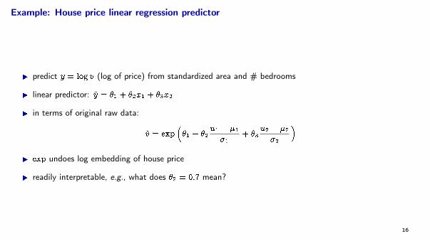
Example: House price linear regression predictor

I predict y = log v (log of price) from standardized area and # bedrooms

I linear predictor: y = �1 + �2x1 + �3x2

I in terms of original raw data:

v = exp��1 + �2

u1 � �1�1

+ �3u2 � �2�2

�

I exp undoes log embedding of house price

I readily interpretable, e.g., what does �2 = 0:7 mean?

16

Vector embeddings

17

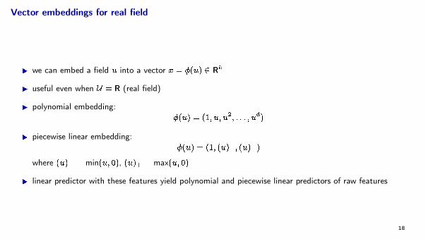
Vector embeddings for real field

I we can embed a field u into a vector x = �(u) 2 Rk

I useful even when U = R (real field)

I polynomial embedding:�(u) = (1; u; u2; : : : ; ud)

I piecewise linear embedding:�(u) = (1; (u)

�

; (u)+)

where (u)�

= min(u; 0), (u)+ = max(u; 0)

I linear predictor with these features yield polynomial and piecewise linear predictors of raw features

18

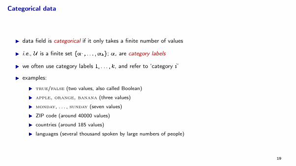
Categorical data

I data field is categorical if it only takes a finite number of values

I i.e., U is a finite set f�1; : : : ; �kg; �i are category labels

I we often use category labels 1; : : : ; k, and refer to ‘category i’

I examples:

I true/false (two values, also called Boolean)

I apple, orange, banana (three values)

I monday, . . . , sunday (seven values)

I ZIP code (around 40000 values)

I countries (around 185 values)

I languages (several thousand spoken by large numbers of people)

19

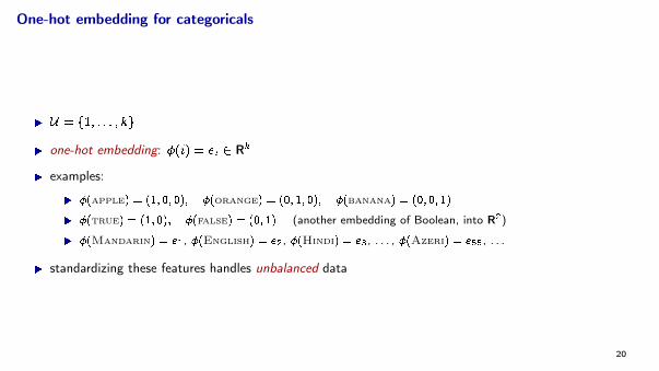
One-hot embedding for categoricals

I U = f1; : : : ; kg

I one-hot embedding: �(i) = ei 2 Rk

I examples:

I �(apple) = (1; 0; 0); �(orange) = (0; 1; 0); �(banana) = (0; 0; 1)

I �(true) = (1; 0); �(false) = (0; 1) (another embedding of Boolean, into R2)

I �(Mandarin) = e1, �(English) = e2, �(Hindi) = e3, . . . , �(Azeri) = e55, . . .

I standardizing these features handles unbalanced data

20

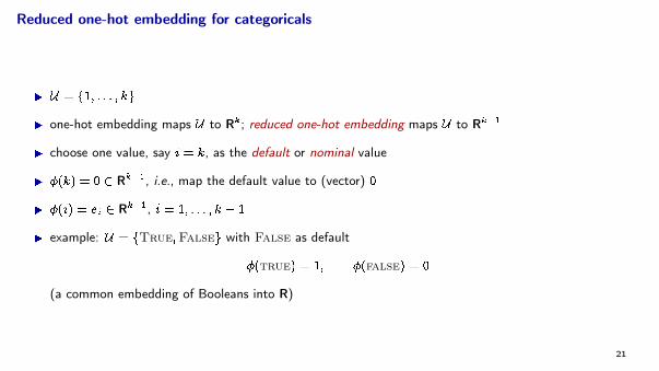
Reduced one-hot embedding for categoricals

I U = f1; : : : ; kg

I one-hot embedding maps U to Rk; reduced one-hot embedding maps U to Rk�1

I choose one value, say i = k, as the default or nominal value

I �(k) = 0 2 Rk�1, i.e., map the default value to (vector) 0

I �(i) = ei 2 Rk�1, i = 1; : : : ; k � 1

I example: U = fTrue;Falseg with False as default

�(true) = 1; �(false) = 0

(a common embedding of Booleans into R)

21

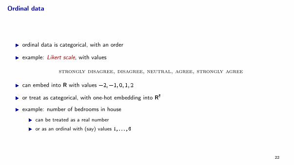
Ordinal data

I ordinal data is categorical, with an order

I example: Likert scale, with values

strongly disagree, disagree, neutral, agree, strongly agree

I can embed into R with values �2;�1; 0; 1; 2

I or treat as categorical, with one-hot embedding into R5

I example: number of bedrooms in house

I can be treated as a real number

I or as an ordinal with (say) values 1; : : : ; 6

22

Feature engineering

23

Feature engineering

I basic idea:

I start with some features

I then process or transform them to produce new (‘engineered’) features

I use these new features in your predictor

I was it a good idea? did it improve your predictor?

I train your model with original features and validate performance

I train your model with new features and validate performance

I if performance with new features is better, your feature engineering was successful

24

Types of feature transforms

I modify individual features: replace original feature xi with modified or transformed feature xnewi

I simple example: standardize, xnewi

= (xi � �i)=�i

I create multiple features from each original feature

I simple example: powers, replace xi with (xi; x2i; : : : ; x

qi)

I create new features from multiple original features

I simple example: product, xnewi

= xkxl

25

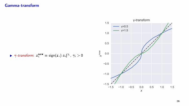
Gamma-transform

I -transform: xnewi = sign(xi)jxij i , i > 0

1.5 1.0 0.5 0.0 0.5 1.0 1.5x

1.5

1.0

0.5

0.0

0.5

1.0

1.5

xnew

-transform

=0.5=1.5

26

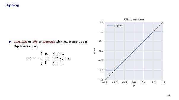
Clipping

I winsorize or clip or saturate with lower and upperclip levels li, ui

xnewi =

8<:

ui xi > uixi li � xi � uili xi < li

1.5 1.0 0.5 0.0 0.5 1.0 1.5x

1.5

1.0

0.5

0.0

0.5

1.0

1.5

xnew

Clip transform

clipped

27

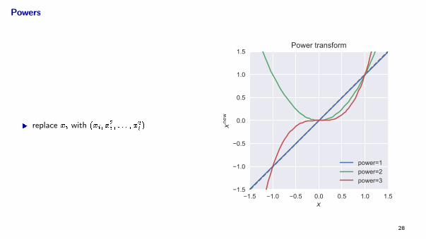
Powers

I replace xi with (xi; x2i ; : : : ; x

qi )

1.5 1.0 0.5 0.0 0.5 1.0 1.5x

1.5

1.0

0.5

0.0

0.5

1.0

1.5

xnew

Power transform

power=1power=2power=3

28

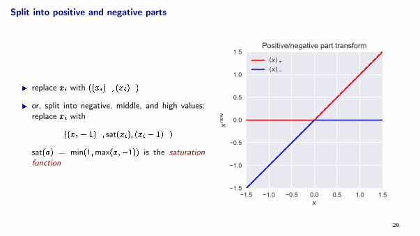
Split into positive and negative parts

I replace xi with ((xi)+; (xi)�)

I or, split into negative, middle, and high values:replace xi with

((xi + 1)�

; sat(xi); (xi � 1)+)

sat(a) = min(1;max(x;�1)) is the saturationfunction

1.5 1.0 0.5 0.0 0.5 1.0 1.5x

1.5

1.0

0.5

0.0

0.5

1.0

1.5

xnew

Positive/negative part transform

(x) +(x)

29

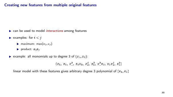
Creating new features from multiple original features

I can be used to model interactions among features

I examples: for i < j

I maximum: max(xi; xj)

I product: xixj

I example: all monomials up to degree 3 of (x1; x2):

(x1; x2; x21; x1x2; x

22; x

31; x

21x2; x1x

22; x

32)

linear model with these features gives arbitrary degree 3 polynomial of (x1; x2)

30

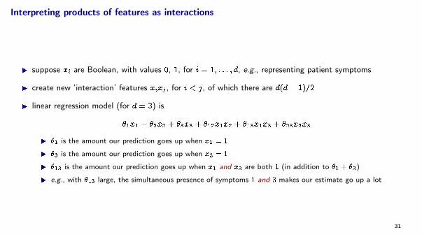
Interpreting products of features as interactions

I suppose xi are Boolean, with values 0, 1, for i = 1; : : : ; d, e.g., representing patient symptoms

I create new ‘interaction’ features xixj , for i < j, of which there are d(d� 1)=2

I linear regression model (for d = 3) is

�1x1 + �2x2 + �3x3 + �12x1x2 + �13x1x3 + �23x2x3

I �1 is the amount our prediction goes up when x1 = 1

I �3 is the amount our prediction goes up when x3 = 1

I �13 is the amount our prediction goes up when x1 and x3 are both 1 (in addition to �1 + �3)

I e.g., with �13 large, the simultaneous presence of symptoms 1 and 3 makes our estimate go up a lot

31

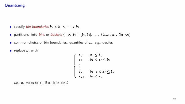
Quantizing

I specify bin boundaries b1 < b2 < � � � < bk

I partitions into bins or buckets (�1; b1]; (b1; b2]; : : : (bk�1; bk]; (bk;1)

I common choice of bin boundaries: quantiles of xi, e.g., deciles

I replace xi with 8>>>><>>>>:

e1 xi � b1e2 b1 < xi � b2...ek bk�1 < xi � bkek+1 bk < xi

i.e., xi maps to el, if xi is in bin l

32

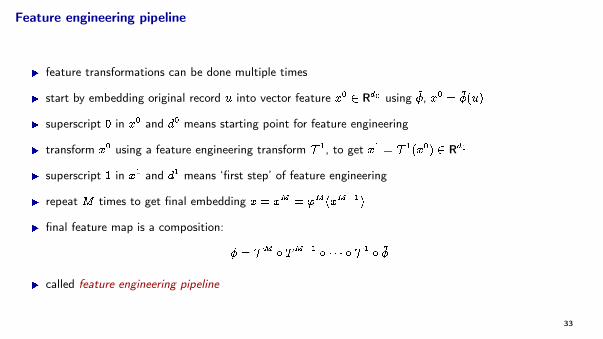
Feature engineering pipeline

I feature transformations can be done multiple times

I start by embedding original record u into vector feature x0 2 Rd0 using ~�, x0 = ~�(u)

I superscript 0 in x0 and d0 means starting point for feature engineering

I transform x0 using a feature engineering transform T 1, to get x1 = T 1(x0) 2 Rd1

I superscript 1 in x1 and d1 means ‘first step’ of feature engineering

I repeat M times to get final embedding x = xM = 'M (xM�1)

I final feature map is a composition:

� = T M � TM�1 � � � � � T 1 � ~�

I called feature engineering pipeline

33

Automatic feature generation

34

Hand crafted versus automatic features

I features and feature engineering described above generally done by hand, using experience

I can also develop feature mappings automatically, directly from some data

I examples: word2vec, vgg16 were developed automatically (from very large data sets)

I we’ll later see some of these methods (PCA, neural nets, . . . )

35

Summary

36

Summary

I raw features are mapped to vectors for subsequent processing

I feature maps can range from simple to complex

I use validation to choose among different candidate feature maps

I sometimes the original feature map is followed by subsequent transformations, called feature engineering

I we’ll see later how feature mappings can be derived from data, as opposed to by hand

37