Sandeep Tata, Richard A. Hankins, and Jignesh M. Patel

Presented by Niketan Pansare, Megha Kokane

Overview Existing Algorithms Motivation Two Approaches Experiments and Analysis

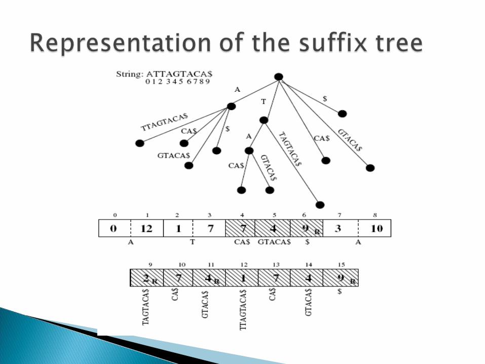
Suffix tree – Compressed trie for nonempty suffixes of a string.

Example Efficient for querying – Exact string

matching = O(length of query)

Weimer McCreight Ukkonen – O(n) – uses suffix links. Starts

from empty tree and inserts suffixes into the partial tree from the longest to shortest suffix.

Pjama – mentioned in previous paper. Deep Shallow – space efficient internal

memory. O(n2 logn).

• Construction of suffix tree for single chromosome - 1.5 hr

• Even though, theoretical complexity of Deep Shallow algo is O(n2 logn) – fastest inmemory algo in practice.

• Problem with previous methods:– Poor locality of reference. High cache miss and

random i/o– Analogy: trying to use internal sorting for array >

memory size. (=> instead of external sorting).

Buffer management strategy for Top Down Disk based (TDD) algo (O(n2))

New Disk based suffix tree construction algorithm that is based on sort-merge paradigm (More efficient than first)

Reduces the main memory requirements through strategic buffering of the largest data structures.

This approach consists of :• A suffix tree construction algorithm, called

‘Partition and Write only Top Down’ (PWOTD)• The related buffer management strategy.

based on the wotdeager algorithm suggested by Giegerich et al.

In PWOTD, the wotdeager algorithm is improved using a partitioning phase which allows one to immediately build larger, independent subtrees in memory.

Consists of 2 phases:• Partitioning• wotdeager algorithm

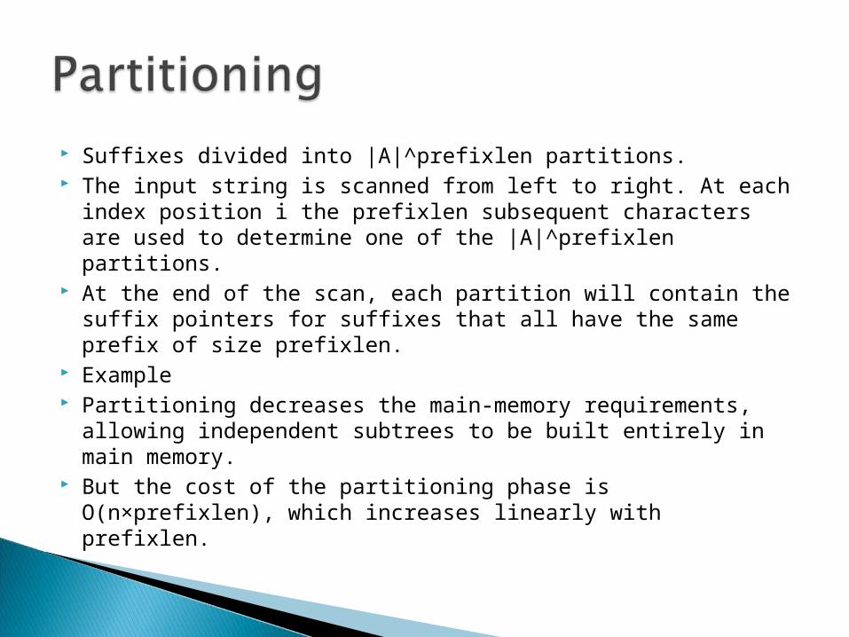
Suffixes divided into |A|^prefixlen partitions. The input string is scanned from left to right. At each index

position i the prefixlen subsequent characters are used to determine one of the |A|^prefixlen partitions.

At the end of the scan, each partition will contain the suffix pointers for suffixes that all have the same prefix of size prefixlen.

Example Partitioning decreases the main-memory requirements,

allowing independent subtrees to be built entirely in main memory.

But the cost of the partitioning phase is O(n×prefixlen), which increases linearly with prefixlen.

4 data structures used: an input string array String, a suffix array Suffixes, a temporary array Temp, and the suffix tree Tree.

The Suffixes array is first populated with suffixes from a partition after discarding the first prefixlen characters.

Illustration

Tree buffer: The reference pattern to Tree consists mainly of sequential writes when the children of a node are being recorded. Occasionally, pages are revisited when an unexpanded node is popped off the stack.

Very good spatial and temporal locality.Hence LRU replacement policy

Suffixes array: Sequential scan to copy into temp array.

And sorted array is written back. There is some locality in the pattern of

writes, since the writes start at each character-group boundary and proceed sequentially to the right.

Hence LRU performs reasonably well

Temp array is referenced in 2 sequential scans:• to copy all of the suffixes in the Suffixes array,

and• to copy all of them back into the Suffixes array in

sorted order. Hence MRU works best for Temp.

String array: smallest main-memory requirement of all

the data structures. But worst locality of access. referenced when performing the count-sort

and to find the longest common prefix in each sorted group.

fairly complex reference pattern, and there is some locality of reference, so both LRU and RANDOM would do well.

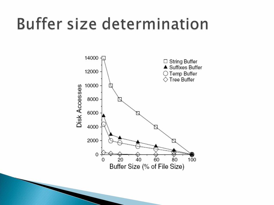
The cache miss behavior for each buffer is approximately linear once the memory is allocated beyond a minimum point.

Once we identify these points, we can allocate the minimum buffer size necessary for each structure. The remaining memory is then allocated in order of decreasing slopes of the buffer miss curves.

Tree needs least amount of buffering due to very good locality of reference.

String needs the most amount of buffer due to very poor locality of reference.

Temp has more locality than suffix

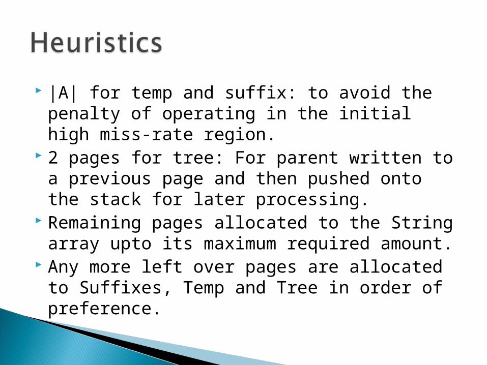
|A| for temp and suffix: to avoid the penalty of operating in the initial high miss-rate region.

2 pages for tree: For parent written to a previous page and then pushed onto the stack for later processing.

Remaining pages allocated to the String array upto its maximum required amount.

Any more left over pages are allocated to Suffixes, Temp and Tree in order of preference.

TDD – inefficient if input strings are significantly greater than the available memory.

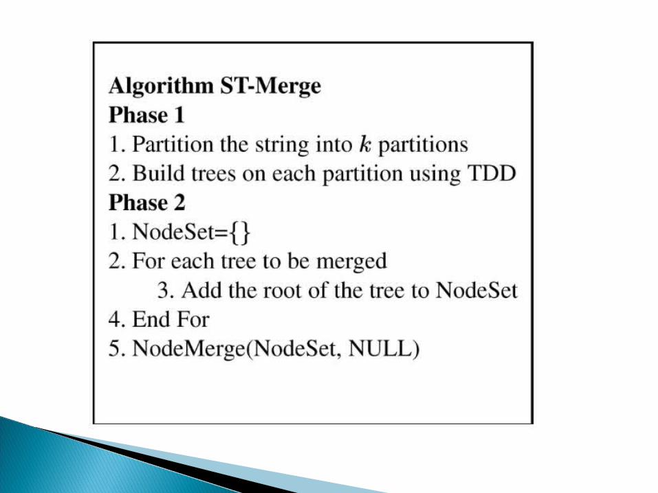
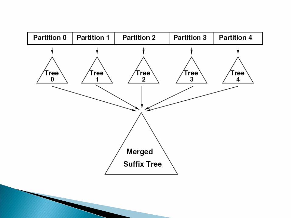
ST-Merge employs divide and conquer strategy similar to the external merge sort algorithm.

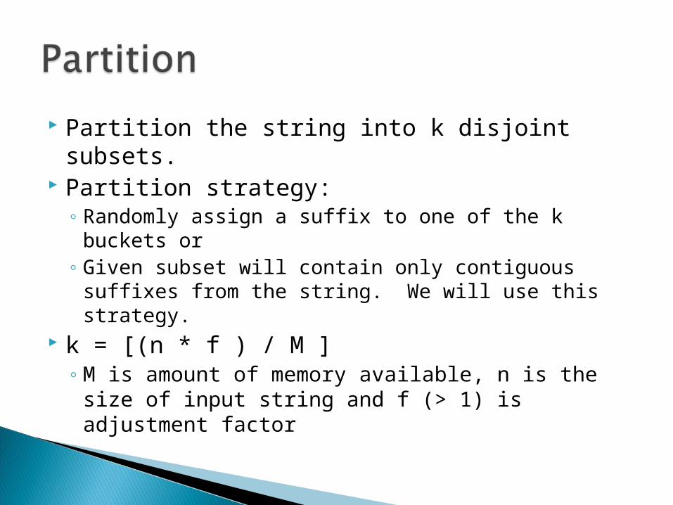
Partition the string into k disjoint subsets. Partition strategy:

◦ Randomly assign a suffix to one of the k buckets or

◦ Given subset will contain only contiguous suffixes from the string. We will use this strategy.

k = [(n * f ) / M ]◦ M is amount of memory available, n is the size

of input string and f (> 1) is adjustment factor

Apply TDD (PWOTD) algorithm on the individual partitions => set of suffix trees.

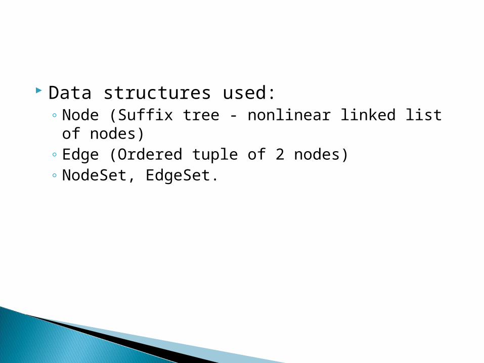
Data structures used:◦ Node (Suffix tree - nonlinear linked list of nodes)◦ Edge (Ordered tuple of 2 nodes) ◦ NodeSet, EdgeSet.

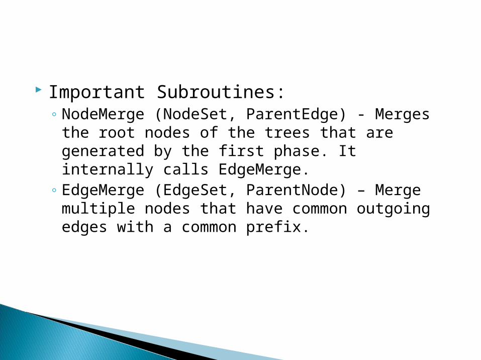
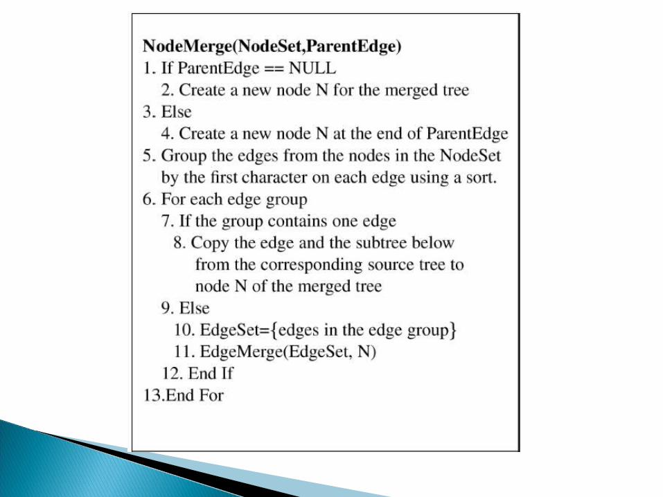
Important Subroutines:◦ NodeMerge (NodeSet, ParentEdge) - Merges the

root nodes of the trees that are generated by the first phase. It internally calls EdgeMerge.

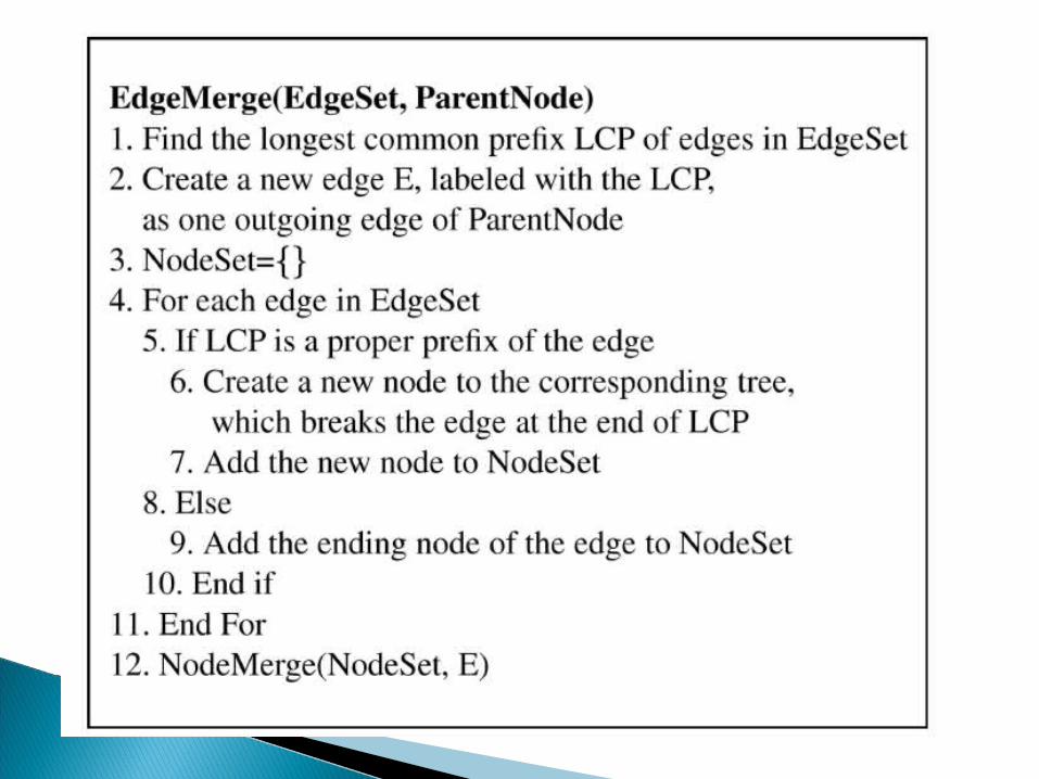
◦ EdgeMerge (EdgeSet, ParentNode) – Merge multiple nodes that have common outgoing edges with a common prefix.

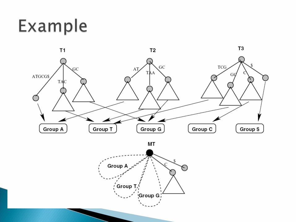
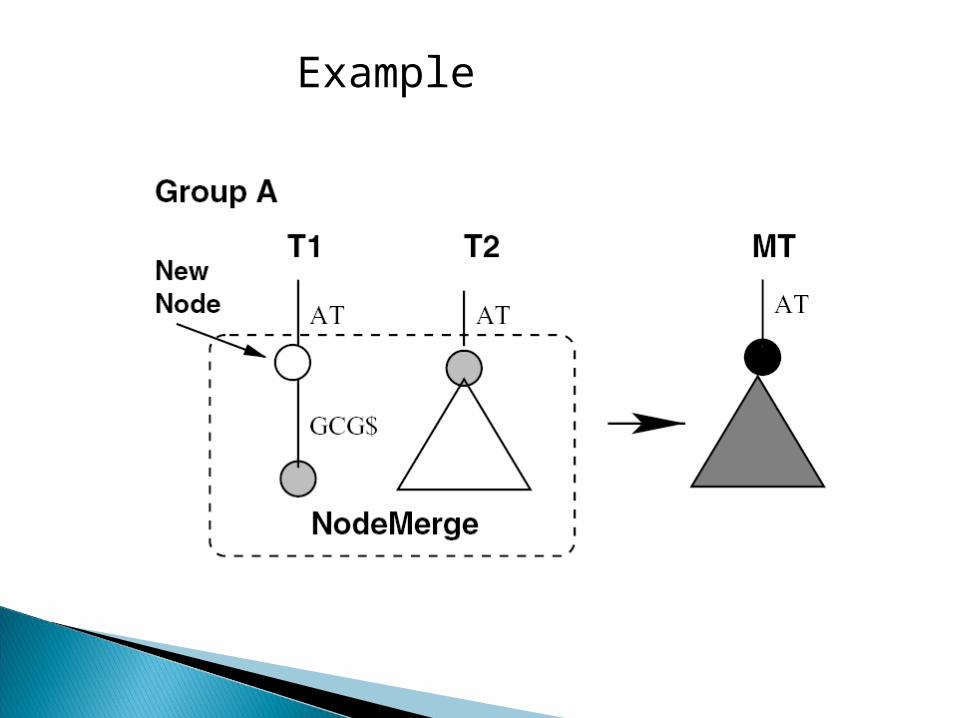
Example

Proper partitioning ensures that most accesses to string are in memory. Therefore, less I/O.

Compared to TDD, the accesses to the string in the second phase have more spatial locality of reference (since smaller working set).

However, if amount of memory is greater than the size of the string, partitioning doesnot provide much benefit, and we simply use TDD.

First Phase: O(n2) Second Phase:

◦ Cost of merging the nodes: O( n * k)◦ Cost of merging the edges : O(n2)

Therefore, the worst case complexity of ST-Merge is O(n2).

Making ST-Merge and TDD to execute parallely.

Using Multiple disk and overlapping I/O and computation.

For source code of TDD, go to http://www.eecs.umich.edu/tdd/download.html

Thank You.