Sampling-based Contact-rich Motion Control

Libin Liu∗∗ KangKang Yin†† Michiel van de Panne‡‡ Tianjia Shao∗ Weiwei Xu†

∗ Tsinghua University † Microsoft Research Asia ‡ University of British Columbia

(a) A forward roll transformed to a dive roll. (b) A cartwheel retargeted to an Asimo-like robot. (c) A walk transformed onto a balance beam.

Figure 1: Physically based motion transformation and retargeting.

Abstract

Human motions are the product of internal and external forces,but these forces are very difficult to measure in a general setting.Given a motion capture trajectory, we propose a method to recon-struct its open-loop control and the implicit contact forces. Themethod employs a strategy based on randomized sampling of thecontrol within user-specified bounds, coupled with forward dynam-ics simulation. Sampling-based techniques are well suited to thistask because of their lack of dependence on derivatives, which aredifficult to estimate in contact-rich scenarios. They are also easyto parallelize, which we exploit in our implementation on a com-pute cluster. We demonstrate reconstruction of a diverse set of cap-tured motions, including walking, running, and contact rich taskssuch as rolls and kip-up jumps. We further show how the methodcan be applied to physically based motion transformation and re-targeting, physically plausible motion variations, and reference-trajectory-free idling motions. Alongside the successes, we pointout a number of limitations and directions for future work.

1 Introduction

Motion capture has been widely used for generating high qualitycharacter animations. However, it remains expensive because of theequipment and space required, as well as frequently requiring te-dious manual post-processing of the data. Contact-rich motions areparticularly difficult to capture and edit afterwards. Self-contactsor occlusions caused by contacts with the environment pose seriousproblems for optical motion tracking systems. Post-processing suchmotions is challenging even for professional animators because of

∗e-mail:{llb05,shaotj08}@mails.tsinghua.edu.cn†e-mail:{kkyin,wwxu}@microsoft.com‡e-mail:van@cs.ubc.ca

the simultaneous existence of many contact constraints. Moreover,manually fixing violated kinematic constraints can easily destroythe physical realism of the original motion. Delicate spatiotemporalrelationships are embedded in the motion dynamics among all thedegrees of freedom (DoFs) for goal-oriented tasks such as rolling.

Reusing and generalizing captured motions or keyframed motionsis the focus of much animation research today [Kovar et al. 2002;Kim et al. 2009]. Of all such efforts, physics-based animation tech-niques promise broader generalizations while preserving physicalrealism [Sok et al. 2007; Yin et al. 2007; Muico et al. 2009; Mac-chietto et al. 2009]. Spacetime trajectory optimizations incorpo-rate physical constraints while searching for or transforming tra-jectories [Witkin and Kass 1988; Liu et al. 2006]. Optimizationwhile tracking reference trajectories during simulations can gen-erate high quality motions [Muico et al. 2009; Macchietto et al.2009]. However, the contact states of the generated motions can-not deviate significantly from the reference trajectory. Proportionalderivative (PD) control coupled with realtime foot placement feed-back can provide robust locomotion, e.g., [Yin et al. 2007], but itis not clear if it generalizes to other tasks. Our goal is to developa general method that can compute controls for multiple types oftasks, some of which do not have well-defined, repeatable contactstates. A caveat will be that our results are computed offline.

We propose to reconstruct the control underlying a motion by cast-ing it as a search problem that seeks to follow a given referencetrajectory. Randomized sampling supports this search by creat-ing a diverse set of motion sequences from which a ‘best track-ing’ path can then be selected. Our use of sampling is inspired bypast successes of sampling-based strategies in robot motion plan-ning [Tsianos et al. 2007], passive animation [Chenney and Forsyth2000; Twigg and James 2007] and active animation [Sims 1994;Wang et al. 2009].

When used for optimization, sampling-based approaches do not de-mand derivative computation, in contrast to gradient-based tech-niques. This is useful when derivatives are hard or impossible tocompute. Many physics-based animation systems are developed ontop of third-party simulators, which can preclude the computationof analytic derivatives. It is also well-known that derivatives are dif-ficult to compute for tasks with abundant transient contacts, such asa roll-and-get-up motion. These contacts pose a serious challengeto inverse dynamics algorithms and gradient-based optimizations.For situations where gradient computations are plausible, gradient-based techniques are nevertheless prone to local minima for highlynonlinear problems in high dimensions. Derivative-free sampling

techniques are not immune to local minima, but they can neverthe-less often escape a local minimum.

When applied to creating motions, a side benefit of sampling-basedmethods is that the stochastic nature of the solution will naturallyexhibit a degree of motion variation. Motion synthesis is often castas an optimization problem, based on the assumption that desiredmotions are optimal in some sense. However, this ignores the nat-ural variations that are evident in human motion. Sampling-basedmethods can also work to achieve a given goal in the absence of areference trajectory, although having one greatly prunes the searchspace and accelerates the construction. This allows us to generatecontrol sequences for non goal-oriented tasks, such as idling, wherea desired trajectory is hard to specify or capture. Sampling schemescan potentially discover new strategies, given enough computa-tional resources.

Sampling-based techniques are also easy to parallelize, which is ofimportance as multi-core computers and compute clusters becomeever more commonplace. We show that control for complex taskscan be reconstructed within minutes on small-scale clusters.

2 Related Work

Motor Control: There are several concepts from the field of motorcontrol that are related to our work: contact dynamics, feedforwardcontrol, and feedback control. Motion and interaction with the en-vironment are fundamentally intertwined. Contact dynamics, or theGround Reaction Force (GRF), is measured and studied intensivelyin medicine and sports. These studies focus on balance and lo-comotion, and analysis rather than synthesis. An interesting recentmethod estimates joint torques and a parametric contact model frommotion [Brubaker et al. 2009]. Internal models represent one ofthe most successful concepts established in neuroscience in recentyears [Kawato 1999; Jordan and Wolpert 1999], and they suggestdecomposing motor control into a feedforward component and afeedback component.

Motion Planning: Motion Planning is a well-studied problem inRobotics. Randomized sampling algorithms for path planning, suchas PRMs (Probabilistic Roadmap Methods) [Kavraki et al. 1996]and RRTs (Rapidly-exploring Random Trees) [LaValle and Kuffner2000] provide significant benefits in speed and robustness over con-ventional deterministic planning algorithms. The computer anima-tion community has adopted these ideas for locomotion planningand manipulation planning [Choi et al. 2003; Yamane et al. 2004].Trajectory planning, also called kinodynamic planning, is a moredifficult task than path planning [LaValle 2006]. A trajectory is apath with a time constraint. Thus while path planning only needs toconsider kinematic constraints, trajectory planning has to take dy-namic constraints into account. In this paper, we reconstruct con-trols to produce plausible trajectories.

Sampling-based Passive Animation: Sampling physically plausi-ble simulations to satisfy user constraints is demonstrated to be ef-fective for passive rigid body systems [Chenney and Forsyth 2000;Twigg and James 2007]. Sampling in a precomputation stage helpsachieve real-time control of deformable objects and fluids at run-time [James and Fatahalian 2003; Barbic and Popovic 2008].

Sampling-based Character Control: More relevant to our work isthe use of local stochastic search and genetic algorithms with built-in randomness that can develop interesting behaviors or morpholo-gies for virtual creatures [Van de Panne and Fiume 1993; Ngo andMarks 1993; Sims 1994]. Stochastic optimization has also beenexplored for constructing and adapting controllers for bipedal lo-comotion [Hodgins and Pollard 1997; Sok et al. 2007; Yin et al.2008]. More recently, sampling-based optimization methods, such

(a) (b)

Figure 2: Collision geometries and DoFs of our character model(a) and robot model (b). Purple dots denote 3-DOF ball joints, andblue spindles denote 1-DOF hinge joints . There are 50 DoFs intotal for the character model, and 35 DoFs in total for the robotmodel, including the global root position and orientation.

as the covariance matrix adaptation strategy, have been shown to beeffective in optimizing walking controllers [Wang et al. 2009] andgenerating optimal gaits and morphologies for animal locomotionwhen combined with traditional derivative-based continuous opti-mization [Wampler and Popovic 2009].

The work of [Sharon and van de Panne 2005; Sok et al. 2007] arethe closest in spirit to our own. Sharon and van de Panne [2005] ap-ply a deterministic coordinate-descent method to optimize the con-trol as best as possible to match target walking motions. The opti-mization proceeds using multiple episodes of increasing simulationduration to deal with overly large search spaces and undesired localminima. Sok et al. [2007] demonstrates control reconstruction for2D locomotion tasks. Their method randomly chooses initial con-figurations and uses a downhill simplex method to find local min-ima. However, the relative benefits of the random initialization andthe local optimization are difficult to quantify, and local optimiza-tion procedures have a sequential nature that makes them hard toparallelize. Our algorithm demonstrates successful reconstructionfor challenging 3D contact-rich motions by focussing its resourcesfully on stochastic sampling.

3 Sampling-based Control Construction

We now detail our sampling-based method for reconstruction of amotion capture trajectory. We begin with a description of the mo-tion data and our character models.

3.1 Motion Data and Character Models

We use motion capture data from the CMU motion capturedatabase, data of published works, data captured by ourselves, andexample trials that came with our motion capture software. Thesemotions demonstrate various tasks and were captured from differ-ent subjects by different groups, with different capture process anddata postprocessing, and contain varying degrees of noise. A con-trol reconstruction method thus needs to be flexible and robust tohandle them all.

Our character model, shown in Figure 2(a), is 1.7m tall and weighs62.5kg. Its detailed kinematic and dynamic parameters can befound in Table 1 and Table 2. To incorporate motion data com-ing from different sources, this biped model has a total of 50 DoFs.Motions captured from different human subjects will be dynami-cally retargeted to this model, directly by our control reconstructionalgorithm, and no kinematic retargeting preprocess is done before-hand. Our Asimo-like robot model, shown in Figure 2(b), is 1.2m

Segment Mass (kg) Inertia (kg ·m2)head 5.494 3.441×10−2,2.210×10−2,3.441×10−2

clavicle & scapula 2.399 5.062×10−3,8.265×10−3,8.265×10−3

upper arm 1.814 2.173×10−3,9.104×10−3,9.104×10−3

lower arm 1.526 1.640×10−3,6.753×10−3,6.753×10−3

hand 0.4588 3.766×10−4,1.597×10−3,1.274×10−3

trunk 14.31 1.300×10−1,1.601×10−1,2.122×10−1

pelvis 4.836 1.620×10−2,4.732×10−2,4.022×10−2

thigh 6.524 8.714×10−2,1.709×10−2,8.714×10−2

shin 4.612 5.565×10−2,8.931×10−3,5.565×10−2

foot 1.612 9.479×10−3,9.706×10−3,1.714×10−3

Table 1: The dynamic properties of our character model.

Joint kp kdStrength Sampling Contact

Scale Window Scaleneck 100 10 1.0, 0.4, 1.0 0.2, 0.2, 0.2

sternoclavicular 300 30 0.1,1.0,1.0 0.1, 0.1, 0.1shoulder 100 5 0.2, 1.0, 1.0 0.2, 0.2, 0.2 3.0

elbow 100 5 0.2, 1.0, 1.0 0.0, 0.0, 0.0 3.0wrist 20 1 0.1, 1.0, 1.0 0.0, 0.0, 0.0 5.0waist 1000 100 0.4, 1.0, 1.0 0.2, 0.2, 0.2hip 300 30 1.0, 0.2, 1.0 0.4, 0.4, 0.1

knee 300 30 1.0 0.2ankle 100 10 1.0, 1.0, 0.5 0.4, 0.2, 0.1 1.0∼5.0

Table 2: The PD control parameters and sampling window size (inRadian) for each DoF of each joint of the character model.

tall and weighs 49.5kg. Its dynamic parameters can be found in Ta-ble 3. We use the triangle meshes rather than geometric primitivesfor collision detection. This robot model has a total of 35 DoFs.

Note that one joint can have up to three DoFs, and the inertia arounddifferent axes are usually not identical. To produce joints that havedifferent strengths in proportion to their associated inertias arounddifferent rotation axes, we scale kp(N/rad) and kd(Ns/rad) withthe scale factors listed in the fourth column of Table 2. Contactscale is used to increase the stiffness of some weight-bearing jointswhen in contact with the ground, to propel the body in certain tasks.For example, the ankle joints can be weak for rolling motions, butneed to be stronger for running, or else the character may not beable to run forward due to a lack of thrust. Alternatively we can usestrong joints all the time, but this can result in stiff-looking motionsand is not in accordance with the changing stiffness observable inhuman muscles and joints.

3.2 Trajectory-based Sampling

3.2.1 Control Representation

We use target poses for PD-servos (Proportional Derivative) to rep-resent motion controls. At every instant of time, the desired angle θ

of a DoF is taken from a desired pose, and the joint torque is calcu-lated as τ = kp(θ−θ)−kd(θ), to drive the current angle θ towardsthe desired value. When there is a reference motion, θi = mi(t) istaken from the trajectory of the corresponding DoF i at the corre-sponding instant of time t.

Naive tracking of a reference trajectory with PD controllers at thejoints is typically unsuccessful for several reasons. First, the cap-tured motions are noisy and sometimes not even physically plau-sible. Second, the kinematic and dynamic properties of our bipedmodel differ from those of the human subjects from whom the mo-tions were captured. Third, there are various modeling errors as-sociated with a rigid body simulator, including driving an oversim-plified rigid biped model with simple PD-servos. We specificallynote two problems of PD-servos. One is that the use of constantkp,kd parameters is problematic for diversified tasks. For exam-

Joint kp kdStrength Sampling Contact

Scale Window Scaleneck 40 4 1.0 0.0

shoulder 100 10 0.15, 1.0, 1.0 0.8, 0.8, 0.25 3.0elbow 100 10 1.0 0.2 3.0wrist 10 1 0.1, 0.4, 1.0 0.0, 0.0, 0.0 3.0hip 500 50 1.0, 0.2, 1.0 0.8, 0.1, 0.4

knee 300 30 1.0 0.6ankle 200 20 1.0, 1.0, 0.5 0.6, 0.6, 0.05 1.0∼3.0

Table 3: The PD control parameters and sampling window size (inRadian) for each DoF of each joint of the robot model.

ple, the shoulder and elbow joints can be relaxed during a walkingmotion. In contrast, if the arms are needed during a motion to sup-port the weight of the whole body, they have to be strong and stiff.Therefore we scale the stiffness and damping parameters accordingto the desired task, as indicated by the last column of Table 2. An-other problem of PD-servos is that they are simplified mechanicalmodels of the complex biological neuromuscular actuation systems.They only react to errors and do not produce feedforward torques.

Because of data noise, model discrepancies, and modeling errors,tracking a reference trajectory directly by PD-servos will usuallyfail to reproduce the desired motion. For example, when trackinga walking motion, the virtual character usually falls within one ortwo steps. When directly tracking a sideways roll, the charactercannot roll more than 40 degrees. It is thus necessary to modifythe reference trajectory properly. Hereafter we denote the referencetrajectory as m, displacements to the reference trajectory as m, andthe simulated motion as m.

3.2.2 Sampling Algorithm and Parallelization

We begin with several definitions. In a multibody system, we de-fine a pose as the aggregation of all the internal joint angles andthe root orientation at a particular time. A sample is defined by apose displacement, that when added to a pose, forms a new pose.For convenience, we also use sample to refer to the displaced newpose. A pose or sample only contains positional information. For adynamically simulated system, we also need to consider the state,which contains both position and velocity information of the sys-tem.

Given a starting state ss on the reference trajectory at time t, wenow consider possible states of the system at time t +∆t. The pos-sibilities are illustrated in Figure 3(a). Given a target state st on thetrajectory at time t +∆t, we can drive the system towards the posesa0 associated with this target state, using PD-servos. The state re-sulting from the simulation, se, however, is likely to drift away fromst . Our algorithm then samples in the vicinity of sa0 to produce newtarget poses sa1,sa2... for advancing the simulation, and a series ofnew end states se1,se2... are generated. We can then select the bestsek, the one closest to st as measured by a cost function to be de-scribed (§3.2.4), and iterate the process using sek as the start state attime t +∆t. Progressively advancing the simulation in this fashionwill eventually return a simulated motion m that is hopefully closeto m.

Due to the curse of dimensionality, and the large number of DoFs ofour model, we need a sufficient amount of samples at each iteration.We denote the number of samples for one iteration as nSample. Be-cause of the existence of noise and model discrepancies, the samplethat achieves the closest end state to the reference state at presentmay not be the best one to select in a longer term. We thereforeretain more than one sample at each iteration until the solution pro-cess has advanced sufficiently far in order to determine which con-trol samples represent the best control sequence. That is, we save

(a) The sampling process.

(b) The sampling process with feedforward offsets.

Figure 3: The basic and modified sampling process.

Figure 4: Schematic illustration of the sampling process with pa-rameters nIter = 5, nSample = 10, and nSave = 2. There are fiveiterations in total, each using ten samples (orange circles), only twoof which are saved (orange dots) and others are discarded. Fromthe two saved samples, ten samples are drawn again. The final cho-sen path is that which has the lowest cost, shown in red.

nSave samples at each iteration. This makes the algorithm morefar-sighted and improves the robustness with respect to the localminima associated with a constrained unstable system. Each endstate associated with the nSave samples from the last time step isthen used as the start state for the next iteration nSample/nSavetimes, so that a total of nSample samples are tested again. Thisprocess is illustrated in Figure 4 with nSample = 10, nSave = 2,and nIter = 5, where nIter denotes the total number of iterations.

From the above description of the sampling process, we can see thatgenerating samples and their associated simulations can be doneconcurrently. Algorithms 1 and 2 describe our parallel implemen-tation of the sampling algorithm. S is an array of length nSample,whose elements consist of all the simulation info (sa,ss,se,c) re-lated to a sample. As before, sa represents a sample, ss the startstate, se its end state, and c is its cost. SM is the two dimensionalnIter× nSave array of the saved samples. From the element ofSM at the last time step of a motion, we backtrack nSave pathsand select the path of minimal cost as the final sample sequencem = (...sa,t , sa,t+∆t , ...).

3.2.3 Practical Implementations

The above section introduces the basic sampling algorithm, whichdoes not work well for a high-dimensional non-linear constrainedsystem that is inherently unstable and discontinuous. We developseveral critical strategies to improve the robustness and speed of the

Algorithm 1 : m = job of master(m,nIter,nSample,nSave)Input: reference motion m; number of iterations nIter; number of samples per iterationnSample; number of saved samples per iteration nSaveOutput: a list of displacement samples m

1: initialize SM[0]2: for t = 1 . . .nIter do3: S = null4: j = 0;k = 0 {initializes counters for sent and received samples}5: while k < nSample do6: while (worker = find idle worker()) == null do7: S = S∪ receive result from worker()8: k++9: end while

10: if j <nSample then11: j++12: ss← pick start state(SM[t−1]) {picks a start state}13: send data to worker(worker,WORK,ss, t)14: end if15: end while16: SM[t] =select samples(S,nSave) {selects only nSave samples}17: end for18: return m← search best path(SM) {returns the path of minimal cost in SM}

Algorithm 2 : calculation of worker(m)Input: reference motion m

1: loop2: (mode,ss, t)=receive data from master()3: if mode! =WORK then4: break5: end if6: sa← generate sample(m, t)7: (m,se)← simulate(ss,sa, m)8: c← calculate cost(m, m)9: send result to master(sa,c,se) {sends the sample, the cost, and the end state}

10: end loop

search algorithm, and the quality of the synthesized motions.

Approximating Feedforward Torques: As mentioned in Sec-tion 3.2.1, there are several factors that can cause the simulationto deviate from the target trajectory during direct PD-tracking. Theforce of gravity is one such factor. If we consider the example ofholding an arm in an extended horizontal position, this will requirea sustained torque at the shoulder. However, a PD-controller willnever reach its desired angle in such a situation because it requiresan error in order to generate a torque. It is possible to rely on thesampling to compensate by adjusting the target position upwards,but this is not always practical in our high-dimensional control set-ting. Instead, we systematically offset sa0 by the pose differencebetween se and st , and sample around s′a0 rather than the originalsa0 instead. This is illustrated in Figure 3(b), which revises the one-dimensional case shown in Figure 3(a). Stated in another way, wecompute an offset to the reference target to approximate feedfor-ward torques, and rely on sampling to generate appropriate torquesthat compensate for noise in the tracking trajectory and model dis-crepancies.

In principle, feedforward torques can be computed using inversedynamics techniques. However, inverse dynamics is extremelychallenging for contact-rich tasks due to the unknown contact lo-cations and contact forces. The proposed offset technique greatlyimproves the success rate of the reconstruction and the quality ofthe resulted control.

Sampling Time Step: The sampling frequency, determined by ∆t,does not have to equal the simulation time step. In fact, it is ad-vantageous to use a lower sampling frequency as long as this doesnot overly constrain the control that can be applied. A low sam-

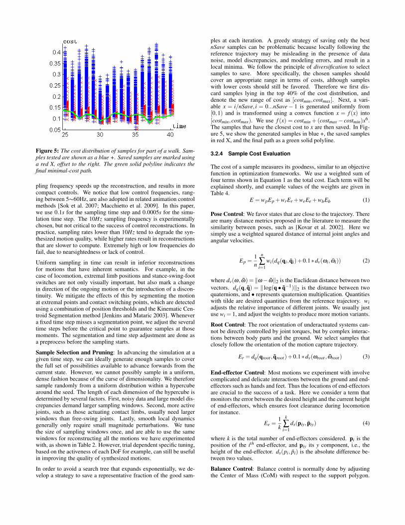
Figure 5: The cost distribution of samples for part of a walk. Sam-ples tested are shown as a blue +. Saved samples are marked usinga red X, offset to the right. The green solid polyline indicates thefinal minimal-cost path.

pling frequency speeds up the reconstruction, and results in morecompact controls. We notice that low control frequencies, rang-ing between 5∼60Hz, are also adopted in related animation controlmethods [Sok et al. 2007; Macchietto et al. 2009]. In this paper,we use 0.1s for the sampling time step and 0.0005s for the simu-lation time step. The 10Hz sampling frequency is experimentallychosen, but not critical to the success of control reconstructions. Inpractice, sampling rates lower than 10Hz tend to degrade the syn-thesized motion quality, while higher rates result in reconstructionsthat are slower to compute. Extremely high or low frequencies dofail, due to nearsightedness or lack of control.

Uniform sampling in time can result in inferior reconstructionsfor motions that have inherent semantics. For example, in thecase of locomotion, extremal limb positions and stance-swing-footswitches are not only visually important, but also mark a changein direction of the ongoing motion or the introduction of a discon-tinuity. We mitigate the effects of this by segmenting the motionat extremal points and contact switching points, which are detectedusing a combination of position thresholds and the Kinematic Cen-troid Segmentation method [Jenkins and Mataric 2003]. Whenevera fixed time step misses a segmentation point, we adjust the severaltime steps before the critical point to guarantee samples at thosemoments. The segmentation and time step adjustment are done asa preprocess before the sampling starts.

Sample Selection and Pruning: In advancing the simulation at agiven time step, we can ideally generate enough samples to coverthe full set of possibilities available to advance forwards from thecurrent state. However, we cannot possibly sample in a uniform,dense fashion because of the curse of dimensionality. We thereforesample randomly from a uniform distribution within a hypercubearound the seed. The length of each dimension of the hypercube isdetermined by several factors. First, noisy data and large model dis-crepancies demand larger sampling windows. Second, more activejoints, such as those actuating contact limbs, usually need largerwindows than free-swing joints. Lastly, smooth local dynamicsgenerally only require small magnitude perturbations. We tunethe size of sampling windows once, and are able to use the samewindows for reconstructing all the motions we have experimentedwith, as shown in Table 2. However, trial dependent specific tuning,based on the activeness of each DoF for example, can still be usefulin improving the quality of synthesized motions.

In order to avoid a search tree that expands exponentially, we de-velop a strategy to save a representative fraction of the good sam-

ples at each iteration. A greedy strategy of saving only the bestnSave samples can be problematic because locally following thereference trajectory may be misleading in the presence of datanoise, model discrepancies, and modeling errors, and result in alocal minima. We follow the principle of diversification to selectsamples to save. More specifically, the chosen samples shouldcover an appropriate range in terms of costs, although sampleswith lower costs should still be favored. Therefore we first dis-card samples lying in the top 40% of the cost distribution, anddenote the new range of cost as [costmin,costmax]. Next, a vari-able x = i/nSave, i = 0...nSave− 1 is generated uniformly from[0,1) and is transformed using a convex function x = f (x) into[costmin,costmax). We use f (x) = costmin +(costmax− costmin)x6.The samples that have the closest cost to x are then saved. In Fig-ure 5, we show the generated samples in blue +, the saved samplesin red X, and the final path as a green solid polyline.

3.2.4 Sample Cost Evaluation

The cost of a sample measures its goodness, similar to an objectivefunction in optimization frameworks. We use a weighted sum offour terms shown in Equation 1 as the total cost. Each term will beexplained shortly, and example values of the weights are given inTable 4.

E = wpEp +wrEr +weEe +wbEb (1)

Pose Control: We favor states that are close to the trajectory. Thereare many distance metrics proposed in the literature to measure thesimilarity between poses, such as [Kovar et al. 2002]. Here wesimply use a weighted squared distance of internal joint angles andangular velocities.

Ep =1n

n

∑i=1

wi(dq(qi, qi)+0.1∗dv(ωi, ωi)) (2)

where dv(ω, ω) = ‖ω− ω‖2 is the Euclidean distance between twovectors. dq(q, q) = ‖ log(q • q−1)‖2 is the distance between twoquaternions, and • represents quaternion multiplication. Quantitieswith tilde are desired quantities from the reference trajectory. wiadjusts the relative importance of different joints. We usually justuse wi = 1, and adjust the weights to produce more motion variants.

Root Control: The root orientation of underactuated systems can-not be directly controlled by joint torques, but by complex interac-tions between body parts and the ground. We select samples thatclosely follow the orientation of the motion capture trajectory.

Er = dq(qroot , qroot)+0.1∗dv(ωroot , ωroot) (3)

End-effector Control: Most motions we experiment with involvecomplicated and delicate interactions between the ground and end-effectors such as hands and feet. Thus the locations of end-effectorsare crucial to the success of a task. Here we consider a term thatmonitors the error between the desired height and the current heightof end-effectors, which ensures foot clearance during locomotionfor instance.

Ee =1k

k

∑i=1

ds(piy, piy) (4)

where k is the total number of end-effectors considered. pi is theposition of the ith end-effector, and piy its y component, i.e., theheight of the end-effector. ds(pi, pi) is the absolute difference be-tween two values.

Balance Control: Balance control is normally done by adjustingthe Center of Mass (CoM) with respect to the support polygon.

We use the relative position of the CoM with respect to each end-effector instead. This has two advantages. First, we do not needto detect support polygons from noisy captured motions. Second,even when an end-effector is not in contact with the ground, its rela-tive position with respect to the CoM still counts. This is importantfor the end-effector to prepare a proper landing position. Once theend-effector has contacted the ground, it is harder to change po-sition anymore. Denote the height of the character as h, and theplanar vector from end-effector i to CoM as rci = (pCoM−pi)|y=0,we calculate the balance deviation as follows:

Eb =1hk

k

∑i=1

(dv(rci− rci))+0.1∗dv(vCoM , vCoM) (5)

3.3 Trajectory-free Sampling for Idle Motions

Idling is common in video games and background movie charac-ters. Although they are usually perceived as easy motions, theirquality is surprisingly low compared to more difficult goal-orientedtasks. Several factors contribute to this phenomenon. One is thatidling is hard to specify procedurally, because there are no cleargoals associated with them, other than a fuzzy feeling that theyshould look relaxed and non-repetitive. There are no obvious cri-teria to constrain idling either. For example, self-collision free isusually a requirement for goal-oriented tasks, but idling is exactlythe opposite and rich in self-contacts. Capturing idle motions isnot popular either. The relatively low importance of idling usuallydoes not justify the high costs associated with motion capture anddata processing. Self-contacts and props like chairs also make cap-ture hard. In the CMU motion capture database, we can only findone very short trial of idling in a chair, while in contrast there aredozens of walking motions. Furthermore, the mocap subject sitsidle very cautiously in this trial, and does not look relaxed at all. Itis indeed problematic for a subject to relax and idle, while wearinga tight suit with 40+ markers on, and being requested to minimizeocclusions between markers or rubbing them with each other. Al-gorithmic studies on idle motions are also very limited. To the bestof our knowledge, the only study on idling dates back more than adecade ago, which is a simple application of Perlin noise on cannedposes and actions [Perlin 1995].

We advocate using randomized sampling for idle motions. In abroader scope, we could sample configurations that look relaxed,i.e., poses that form multiple self-contacts and contacts with a sup-porting object, and require low joint torques to maintain. In thiswork, we restrict ourselves to a more specific scenario where a userspecifies a set of key poses, from which our algorithm constructscontrollers to drive the character to idle in-between. Unlike con-trol reconstruction from mocap trajectories, here we only have keyposes but no reference trajectory. The key challenge for such analgorithm is again the high-dimensionality of the state space. Wedevelop a control planning algorithm based on RRT [LaValle andKuffner 2000], one of the state-of-art path planning methods, withseveral crucial modifications:

• In the initialization phase, all the input key poses are simu-lated with low-gain PD controllers, to generate relaxed poseswhich form multiple contacts with the supporting furniture.The relaxed poses will replace the original poses as input toRRT.

• During initialization, a start state is directly driven to a targetstate by PD servos. DoFs that can reach the target are removedfrom RRT to reduce the dimensionality for sampling.

• In the EXTEND operation, control targets are sampled, notfrom the whole configuration space but from a hyper tubearound the spherical linear interpolation of the start and goalstates, to limit the sampling space.

• The character is simulated towards a sampled target withina time frame proportional to the distance between states.This step implicitly eliminates undesired collisions but retainsvalid contacts.

To generate motion variations, we compute multiple trajectories be-tween each pair of key poses. Then as a postprocess, we manuallyselect the best trajectories from all sampled controls, and performsimple algorithmic path simplification and smoothing, similar inspirit to that of [Yamane et al. 2004], but only to the extent wherecontrol permits. More specifically, because of the dynamic natureof our planned controllers, there is no guarantee that an edited con-troller will still work after nodes are removed or smoothed. A con-troller is tested automatically after every modification, and a failureto reach the target revokes the operation just performed. At run-time, we add a small amount of random noise to the controls. Thiseffectively eliminates zombie-looking fully static poses, and addsmore variations to the synthesized motions. Another option hereis to use Perlin noise, but we find simple random noise works justfine.

RRT-based path planning has been used for synthesizing manipu-lation tasks [Yamane et al. 2004]. Their method samples the end-effector configurations and relies on inverse kinematics to solve forjoint angles. We directly sample from the pose space. Another dif-ference is that they use RRT in its original kinematic form, whilewe perform a kind of dynamic RRT where the controls are sampleddirectly. This partly explains the reasonable quality of our simu-lated motions even without the velocity profile fitting component oftheir approach. The lack of stereotypical styles, preferred trajecto-ries, and bell-shaped velocity profiles in idling is likely the otherfactor that makes velocity profile fitting unnecessary in our case.

4 Results

We use the Open Dynamics Engine (ODE) version 0.11 to simu-late our characters. The simulation time step is 0.0005s and thecoefficient of friction is 0.8. The simulation runs at approximatelyreal-time rates on an Intel Xeon E5520@2.27GHz desktop.

Control Reconstruction: We have reconstructed controls for var-ious tasks, some of which are listed in Table 4. To the best of ourknowledge, contact-rich rolling motions have never been consid-ered by previous automatic control reconstruction methods. Table 4also shows representative reconstruction times of various trials ona small cluster of 80 cores, using 1400 samples for each iteration.The reconstruction is quite robust with respect to noise in input data.Occasionally we have mocap trials that have knees bending back-wards severely, or hands flipping around etc. We can still success-fully reconstruct control for them, but the simulated motions havethese noisy artifacts too, mainly due to the tracking nature of thereconstruction algorithm.

Although the tasks we have tested are different, we are able to re-construct controls for all of them using one set of sampling and sim-ulation parameters, as shown in Table 2 and Table 4. Manual tuningof these parameters is necessary, but it was not difficult in our expe-rience. We did not find the results to be highly sensitive to specificweighting of the terms in the cost function in Equation 1. We canuse the same set of weighting, wp = 8,wr = 5,we = 20,wb = 20for example, to reconstruct controls for all the motions. Remainingvariations in the given parameters and weights are largely an artifactof experimentation with progressively more diverse motions, withthe final set of weights typically being backwards compatible withthe original smaller starting set of motions. Although the balanceterms are not necessary for tasks where balance does not play animportant role, a sideways roll for example. Task-specific tuning of

Trial Duration nIter Reconstruction Time wp,wr ,we,wb

walk 5.2 62 143 5, 3, 30, 10run 2.0 27 51 8, 5, 30, 20

sideways roll 3.0 30 78 8, 5, 0, 0forward roll 3.0 30 78 8, 5, 0, 20

backward roll 2.1 21 57 8, 5, 0, 20get-up 3.5 40 93 8, 5, 20, 20kip-up 6.6 66 184 8, 5, 20, 20

Table 4: Performance statistics: Timing units are in seconds.nIter correlates with the duration of motion. nSample = 1400 andnSave = 200. The cluster consists of 10 computational nodes, andeach node consists of two Quad-Xeon (E54xx) processors.

Trial Duration nIter Reconstruction Time wp,wr ,we,wb

walk 5.2 62 193 5,3,30,10run 2.0 27 80 8,5,30,20

sideways roll 3.0 30 133 8,5,0,0forward roll 3.0 30 109 8,5,0,20

backward roll 2.1 21 75 8,5,0,20get-up 3.5 40 140 8,5,20,20kip-up 4.3 43 165 8,5,20,20

cartwheel roll 2.1 21 50 2,10,0,0

Table 5: Performance statistics on the same compute cluster for theAsimo-like robot model. Timing units are in seconds. nSample =2000 and nSave = 500.

the weights is possible if the user wishes to emphasize or deempha-size particular terms. For instance, the end-effector term is used tomatch the height of the feet better for locomotion tasks, but can bedisabled for rolling tasks where the user does not care.

nIter correlates with the duration of motion, the sampling time step,and the segmentation method used, as described in Section 3.2.3.When uniform sampling is used, nIter equals the duration of mo-tion divided by the sampling time step, which is the case for rolling.For locomotion tasks, semantic segmentation is also used, and thatadds more sampling iterations at contact switching and visually im-portant instants of the motion. The contact scale parameters in Ta-ble 2 are never used for rolling. Walking uses an ankle contact scale1.0; running uses an ankle contact scale 5.0; and the get-up motionuses a contact scale 3.0 for the shoulders and the elbows, and 5.0for the wrists.

Even though the reconstruction algorithm is quite robust, there isno guarantee that every episode of sampling can produce successfulcontrols, due to its randomness. The successful rate is quite high,however, for most trials we have experimented. An input motionwith a large feasible region of control, such as the sideways roll,succeeds almost every time. The most challenging trial is one ofthe get-up motions, where the character fails to stand up two thirdsof the time with nSample = 1400 and nSave = 200. The originalmocap trial actually looks like the subject just made it. However,the failure rate decreases to one fourth if we use nSample = 4000and nSave = 400.

In the accompanying video, we show that multiple runs of the sam-pling algorithm produce slightly different controls and simulatedmotions. Note that in [Lau et al. 2009], statistical generative mod-els are learned from multiple trials of the same motion to producemotion variants for walking, swimming etc. We only need oneexample trial, and can produce physically-plausible motions withrapidly-changing contacts. Furthermore, application of the pro-posed reconstruction method is not limited to biped models. Weuse an animation sequence extracted from a wildlife footage [Lau-rent et al. 2004], and reconstruct a running controller for a Cheetahmodel. Imaginary characters with non-standard morphology shouldpose no problem either.

Figure 6: Rolling on hard floor (left) and soft material (right). Notethe difference in contacts and pressure.

Figure 7: Keypose-based control construction. Input poses (top)and simulated motions (bottom).

Motion Transformation: The inherent robustness of the samplingapproach enables straightforward physically based motion transfor-mation. Most of the reference mocap moves we use were capturedinside controlled lab environments, and we test the algorithm withinmore challenging settings, or environments with altered physicalparameters. For example, we reconstruct a normal walk on a groundwith pebbles of random sizes scattered at random locations. Thefeet adapt to the uneven ground naturally. The same motion is alsomade to walk on an icy surface with a coefficient of friction 0.1. Thefeet slide realistically, with the balance automatically maintainedby the reconstructed controls. In a balance beam walking test, wemanually displace the lower-body trajectory of a mocap walk sothat it walks on a straight line. Then we reconstruct the walk on a10cm-wide and a 5cm-wide balance beam, and the sampling suc-ceeds in both cases with correct balancing behaviors added. Thesetransformed motions are likely difficult to be captured or manuallydesigned.

Without any difficulty, we can reconstruct the forward rolling witha ramp of 10 degrees, or a 10cm height raise, or a 50cm height dropput in front of the character. More adverse conditions, such as a100cm height drop shown in Figure 1(a), do not necessarily defeatthe reconstruction. But the character plunges too fast and lands onits back in the synthesized motion, whereas in real life a martialartist would control the timing of the fall to land on his hands first.This problem is caused by the tracking nature of our reconstruction.On the other hand, if simple editing of the reference trajectory isaffordable, we can easily slow down the diving part of the inputdata so that the reconstructed control can land the virtual characteron its hands.

Sometimes it is desired to be able to inspect the distribution of con-tacts and pressure during the course of a motion, for martial artseducation or biomechanical applications such as injury analysis andproduct design [Payton and Bartlett 2007]. We can reproduce themovement of contacts and the change of pressure by simulatingfrom reconstructed controls, as shown in Figure 6. We further re-

Figure 8: A sideways roll captured from human retargeted to an Asimo-like robot.

Figure 9: An example interaction with the virtual character. The character gets pushed and falls, rolls sideways, gets up, gets pushed again,rolls backwards, and gets up again.

construct controls for the roll on a springy crash pad, simulated bysetting the error reduction parameter to 0.8 and the constraint forcemixing parameter to 0.007 in ODE. The two snapshots in Figure 6are taken at the same instant of the roll. As we can see, the rollingon the soft material lags behind a little, with more contact pointseach of less pressure. We speculate that the sampling algorithmwill also be effective in a real deformable body simulator.

Motion Retargeting: Motion retargeting usually refers to the pro-cess of editing an existing motion for a new kinematic model sothat kinematic constraints and effects are maintained or meaning-fully adapted. Our control reconstruction process can achieve dy-namic motion retargeting, where dynamic effects as well as kine-matic constraints are adapted. We retarget various motions cap-tured from human subjects to the Asimo-like robot model shownin Figure 2(b). These retargeting tasks are extremely challengingbecause of the huge differences between the human subjects andthe Asimo model, in terms of their kinematic parameters, dynamicparameters, and collision detection geometries. Nonetheless, thesampling-based algorithm succeeds in reconstructing controls formost of the motions, such as the cartwheel shown in Figure 1(b)and the barrel roll shown in Figure 8. The performance statistics isgiven in Table 5.

The root positions of the original mocap data are simply linearlyscaled down for Asimo using the ratio of body heights, so there aremany severe ground penetrations and floating moves in the refer-ence trajectories. However, we are able to eliminate these in thesynthesized motions, without any kinematic retargeting preprocess,although the synthesis quality might be degraded because of this.Compared to reconstructions on the character model, the controlsreconstructed on the Asimo model require larger sampling win-dows, produce motions of lower quality, and are less accurate interms of trajectory tracking. For example, due to wider and boxylegs, and the lack of a waist joint, Asimo cannot twist its spine or itslegs around each other like humans do, and has to rely on a shoul-der strategy to roll sideways. The Asimo running is quite sluggish,mostly because Asimo has bent knees defined for its T-pose, whichcauses early touchdown of the feet when the knees extend duringlocomotion. We were not able to successfully reconstruct controlsfor the backward roll on Asimo. We suspected that it is becauseAsimo only has a one-DoF neck joint. We temporarily assignedthree-DoFs to Asimo’s neck, and then are able to produce a suc-cessful backward roll from the sampled controls.

Idling: We test the trajectory-free control construction with anidling-in-chair scenario. A few input example poses, such as the toprow of Figure 7, can generate relaxing motions with subtle move-ments. In the accompanying video, we compare the sit idle mo-tion synthesized from our algorithm, an artist designed animationclip, and a motion capture trial. We deem the quality of the syn-thesized motion comparable, if not better than, the quality of idlinganimations from the other two sources. In many cases people havethought our synthesized idling was motion captured. We encour-age the readers to watch the accompanying video and evaluate thequality yourself. In addition, with the constructed controls, we caneasily simulate dynamic effects such as rocking back and forth in arocker, shown in the bottom row of Figure 7.

Motion Composition: To support interactive applications suchas video games, we need to compose controls individually con-structed [Faloutsos et al. 2001]. However, our reconstructed con-trols are open-loop in nature. That is, for each reference motion m,the reconstructed control produces a simulated trajectory m, calledthe canonical trajectory from now on. When starting from a statenot on the canonical trajectory, either as a result of external pertur-bations or changed environments, the virtual character is unlikelyto follow m to accomplish the planned task. Previous methods forconstructing feedback laws are either task-dependent, or not robustenough for our target application [Yin et al. 2007; Muico et al.2009]. Another possibility is to construct dense control policies asin [Sharon and van de Panne 2005; Sok et al. 2007], yet the memoryrequirement of these systems, when applied to many tasks as in ourcase, is too high for console games.

We thus use a hybrid approach to transition between controls.Within every m, we select cut points where other controllers cantransition into. When there is no disturbance, motions are simulatedor transitioned dynamically as planned. Upon external perturba-tions, the current controller still acts as planned for another 200ms,to approximate the reaction time in biological systems. Then theperturbed state, most likely far away from m already, is comparedwith all the cut points of all the controllers. If a close cut point ex-ists, we simply switch to simulate from the matching cut point, andkinematically blend the end state resulted from the perturbation intothe new canonical trajectory. If no close cut point can be found, asemi-ragdoll controller takes over, and produces simple reflex-likebehaviors, such as arm extensions, for fall protection. Transitionscan still be made anytime during the ragdoll controller, if a suitable

cut point can be found. An example would be a transition into abackward roll during the course of a backward fall. In most cases,however, the character just collapses to the ground, and looks for aproper get-up controller to transition into. PD control is then usedto drive the character close to the canonical trajectory of the chosenget-up controller, which will then take over.

Figure 9 is one example interaction with our virtual character. Notethat when the character is acting as planned, we can in theory justkinematically play back the captured motions, similar to the ap-proach of [Zordan et al. 2005]. An extra kinematic retargeting pro-cess is needed, however, to transform all the data captured frompeople of different sizes and proportions to the same biped model.In addition, we choose to always simulate, to avoid the constantswitching back and forth between a kinematic controller and a dy-namic one.

5 Discussion

We introduce the use of randomized sampling to tackle controlproblems for contact-abundant motions such as rolling and idling.We also present practical design choices and efficient parallel algo-rithms to realize an interactive, workable algorithm. As with otherhigh dimensional problems, the specific design choices related torepresentation and implementation play a critical role in develop-ing a working system. The robustness and flexibility of the schemeare demonstrated through physics-based motion transformation andretargeting, and on different kinematic and dynamic models.

Scalability: The proposed algorithm scales almost linearly withrespect to the number of available cores. With our 80-core computercluster, the current implementation requires approximately 25s ofwall-clock time to reconstruct 1s of motion. With an additionalorder of magnitude of increase in the number of cores, an artist canpotentially work with the system at interactive speed. This may berealized with the help of architectures such as the Amazon ElasticComputing Cloud, which allow for the dynamic allocation of largescale computing resources.

Robustness of Reconstruction: Our method is not an optimiza-tion, so there is no convergence problem. The algorithm returnswithin a fixed amount of time, given a set of sampling parametersand a particular motion. The reconstructed control is not guaranteedto be successful, however, after a single run of the sampling algo-rithm. A failure means falling while walking, unable to turn overwhile rolling etc. Our experiments show high success rates though.Roughly speaking, > 80% of the reconstructions finish with a suc-cess rate of > 80%. Furthermore, because each reconstruction runrequires only minutes, the algorithm can be run multiple times onthe same problem to allow a user to explore different possible re-constructions. Another option is to increase the number of drawnsamples and saved samples at each iteration.

We have succeeded for all the motions we tried with the humanmodel. In retrospect, the rich contacts probably help us in someways in counteracting drifts and errors. It would be interesting to tryour method on aerial motions where we cannot do anything aboutdrifts for long durations. In the future, we also wish to add a back-tracking ability to the sampling algorithm. This would help pre-clude making decisions that appear to be good in the short term butturn out to be bad ones later on. In case offsprings of bad sampleshave driven away all descendants of good samples during samplepruning, it would be desirable to rewind to previous iterations andresample to make up the mistake. This strategy is likely to furtherimprove the success rate of reconstruction.

Robustness of Control: Our ‘control bases’ are fixed in time,meaning that control actions are time-dependent but not state-

dependent. Put it another way, the controls we construct are open-loop. Although this provides a solution to inverse dynamics andmotion transformation for contact-abundant motions, the controlsare not robust with respect to external perturbations or environmen-tal changes. We can try to search for dense control policies, i.e.,mappings between states to actions, as in [Sharon and van de Panne2005; Sok et al. 2007]. But this is likely difficult because of the ex-istence of a myriad of local minima caused by many fast-changingcontacts. A more promising avenue is to build task-dependent, ac-tive feedback mechanisms to form close-loop controllers as in [Yinet al. 2007]. This may or may not be possible for certain types oftasks.

Generalization: One of the major motivations for physics-based motion synthesis techniques is to generalize motion cap-ture data [Zordan and Hodgins 2002; Yin et al. 2003]. We havedemonstrated several forms of motion generalization within thesame framework, and it is interesting to think about how to pushthem even further. (a) motion cleanup: Contact-rich motions arehard to capture and clean up. Some of the input trajectories weuse have serious contact flaws, like ground penetrations and con-tact sliding. Our method currently can correct penetrations but notsliding. We can experiment with adding another term into the costfunction to penalize sliding and other artifacts in the input that wewish to get rid of. (b) motion variation: We focus on small vari-ations that can be treated as noise, similar to what is modeled in[Lau et al. 2009]. That is, the same person in the same physical andmental conditions still cannot reproduce his last motion exactly. Formotion variations caused by other reasons, such as mood changes orphysical injuries, new mechanisms have to be devised. (c) motiontransformation: Because of the tracking nature of the trajectory-based sampling, our motion transformations cannot deviate too faraway from the input trajectory. To achieve even larger transforma-tions, we recommend using a controller adaptation scheme, suchas [Yin et al. 2008], on the reconstructed controls rather than holdon to the reference trajectory all the time. Manual editing of theinput trajectories can also help shape the synthesized motions. (d)motion retargeting: The Asimo model differs significantly from thehuman model, and if the model were to differ more, at some pointthe retargeting would simply fail. Continuation methods may behelpful for more aggressive retargeting.

Smoothness of Motion: In our method, samples are independentlydrawn and there is currently no mechanism to control the smooth-ness of the synthesized motion. This can result in the introductionof noise into the synthesized motion. It is not problematic for mo-tions such as rolling because of the changing pattern of collisions,but can be noticeable for other classes of motions, such as the free-swinging arms in a balance beam walk. In such cases we proposeusing a butterworth filter to post-process the generated motion. An-other alternative would be to add a smoothness term when evaluat-ing the sample cost.

Acknowledgements: We would like to thank the anonymous re-viewers for their constructive comments. We thank all our motioncapture subjects, students who helped post-process the data, andorganizations and authors who generously shared their motion cap-ture data. We thank Xiao Liang and Teng Gao for helping us withcoding on the HPC cluster; Kevin Loken for helpful advice on anumber of occasions.

References

BARBIC, J., AND POPOVIC, J. 2008. Real-time control of physi-cally based simulations using gentle forces. ACM Trans. Graph.27, 5.

BRUBAKER, M. A., SIGAL, L., AND FLEET, D. J. 2009. Esti-mating contact dynamics. In IEEE International Conference onComputer Vision (ICCV).

CHENNEY, S., AND FORSYTH, D. A. 2000. Sampling plausiblesolutions to multi-body constraint problems. In SIGGRAPH ’00:Proceedings of the 27th annual conference on Computer graph-ics and interactive techniques, 219–228.

CHOI, M. G., LEE, J., AND SHIN, S. Y. 2003. Planning biped lo-comotion using motion capture data and probabilistic roadmaps.ACM Trans. Graph. 22, 2, 182–203.

FALOUTSOS, P., VAN DE PANNE, M., AND TERZOPOULOS, D.2001. Composable controllers for physics-based character ani-mation. In Proceedings of SIGGRAPH 2001, 251–260.

HODGINS, J. K., AND POLLARD, N. S. 1997. Adapting simulatedbehaviors for new characters. In SIGGRAPH ’97: Proceedingsof the 24th annual conference on Computer graphics and inter-active techniques, 153–162.

JAMES, D. L., AND FATAHALIAN, K. 2003. Precomputing in-teractive dynamic deformable scenes. In SIGGRAPH ’03: ACMSIGGRAPH 2003 Papers, 879–887.

JENKINS, O., AND MATARIC, M. 2003. Automated derivationof behavior vocabularies for autonomous humanoid motion. In2nd International Joint Conference on Autonomous Agents andMultiagent Systems (AAMAS).

JORDAN, M. I., AND WOLPERT, D. M. 1999. Computationalmotor control. In The Cognitive Neurosciences, M. Gazzaniga,Ed. MIT Press.

KAVRAKI, L. E., SVESTKA, P., LATOMBE, J.-C., AND OVER-MARS, M. H. 1996. Probabilistic roadmaps for path planningin high-dimensional configuration spaces. IEEE Transactions onRobotics & Automation 12, 4, 566–580.

KAWATO, M. 1999. Internal models for motor control and trajec-tory planning. Current Opinion in Neurobiology 9, 718–727.

KIM, M., HYUN, K., KIM, J., AND LEE, J. 2009. Synchronizedmulti-character motion editing. ACM Trans. Graph. 28, 3.

KOVAR, L., GLEICHER, M., AND PIGHIN, F. 2002. Motiongraphs. In SIGGRAPH ’02: Proceedings of the 29th annual con-ference on Computer graphics and interactive techniques, ACM,New York, NY, USA, 473–482.

LAU, M., BAR-JOSEPH, Z., AND KUFFNER, J. 2009. Model-ing spatial and temporal variation in motion data. ACM Trans.Graph. 28, 5.

LAURENT, F., LIONEL, R., CHRISTINE, D., AND MARIE-PAULE,C. 2004. Animal gaits from video. In SCA ’04: Proceedings ofthe 2004 ACM SIGGRAPH/Eurographics symposium on Com-puter animation, 277–286.

LAVALLE, S. M., AND KUFFNER, J. J. 2000. Rapidly-exploringrandom trees: Progress and prospects. In Proceedings Workshopon the Algorithmic Foundations of Robotics.

LAVALLE, S. M. 2006. Planning Algorithms. Cambridge Univer-sity Press.

LIU, C. K., HERTZMANN, A., AND POPOVIC, Z. 2006. Com-position of complex optimal multi-character motions. In SCA’06: Proceedings of the 2006 ACM SIGGRAPH/Eurographicssymposium on Computer animation, Eurographics Association,215–222.

MACCHIETTO, A., ZORDAN, V., AND SHELTON, C. R. 2009.Momentum control for balance. ACM Trans. Graph. 28, 3.

MUICO, U., LEE, Y., POPOVIC, J., AND POPOVIC, Z. 2009.Contact-aware nonlinear control of dynamic characters. ACMTrans. Graph. 28, 3.

NGO, J. T., AND MARKS, J. 1993. Spacetime constraints revisited.In Proceedings of SIGGRAPH 1993, 343–350.

PAYTON, C., AND BARTLETT, R. 2007. Biomechanical Evalua-tion of Movement in Sport and Exercise. Routledge.

PERLIN, K. 1995. Real time responsive animation with personality.IEEE Transactions on Visualization and Computer Graphics 1,1, 5–15.

SHARON, D., AND VAN DE PANNE, M. 2005. Synthesis of con-trollers for stylized planar bipedal walking. In ICRA05, 2387–2392.

SIMS, K. 1994. Evolving virtual creatures. In Proceedings ofSIGGRAPH 1994, 15–22.

SOK, K. W., KIM, M., AND LEE, J. 2007. Simulating bipedbehaviors from human motion data. ACM Trans. Graph. 26, 3,Article 107.

TSIANOS, K. I., SUCAN, I. A., AND KAVRAKI, L. E. 2007.Sampling-based robot motion planning: Towards realistic appli-cations. Computer Science Review 1 (August), 2–11.

TWIGG, C. D., AND JAMES, D. L. 2007. Many-worlds browsingfor control of multibody dynamics. ACM Trans. Graph. 26, 3.

VAN DE PANNE, M., AND FIUME, E. 1993. Sensor-actuator net-works. In Proc. ACM SIGGRAPH, ACM, 335–342.

WAMPLER, K., AND POPOVIC, Z. 2009. Optimal gait and formfor animal locomotion. ACM Trans. Graph. 28, 3, Article 60.

WANG, J. M., FLEET, D. J., AND HERTZMANN, A. 2009. Op-timizing walking controllers. ACM Trans. Graph. 28, 5, Article168.

WITKIN, A., AND KASS, M. 1988. Spacetime constraints. InProceedings of SIGGRAPH 1988, 159–168.

YAMANE, K., KUFFNER, J. J., AND HODGINS, J. K. 2004. Syn-thesizing animations of human manipulation tasks. ACM Trans.Graph. 23, 3, 532–539.

YIN, K., CLINE, M. B., AND PAI, D. K. 2003. Motion pertur-bation based on simple neuromotor control models. In PG’03:Proceedings of the 11th Pacific Conference on Computer Graph-ics and Applications, 445–449.

YIN, K., LOKEN, K., AND VAN DE PANNE, M. 2007. Simbicon:Simple biped locomotion control. ACM Trans. Graph. 26, 3,Article 105.

YIN, K., COROS, S., BEAUDOIN, P., AND VAN DE PANNE, M.2008. Continuation methods for adapting simulated skills. ACMTrans. Graph. 27, 3, Article 81.

ZORDAN, V. B., AND HODGINS, J. K. 2002. Motion capture-driven simulations that hit and react. In ACM SIGGRAPH Sym-posium on Computer Animation, 89–96.

ZORDAN, V. B., MAJKOWSKA, A., CHIU, B., AND FAST, M.2005. Dynamic response for motion capture animation. ACMTrans. Graph., 697–701.