1

Foundations of Computer Graphics (Fall 2012)

CS 184, Lectures 19: Sampling and Reconstruction

http://inst.eecs.berkeley.edu/~cs184

Acknowledgements: Thomas Funkhouser and Pat Hanrahan

Outline

§  Basic ideas of sampling, reconstruction, aliasing

§  Signal processing and Fourier analysis

§  Implementation of digital filters

§  Section 14.10 of FvDFH (you really should read)

§  Post-raytracing lectures more advanced topics §  No programming assignment §  But can be tested (at high level) in final

Some slides courtesy Tom Funkhouser

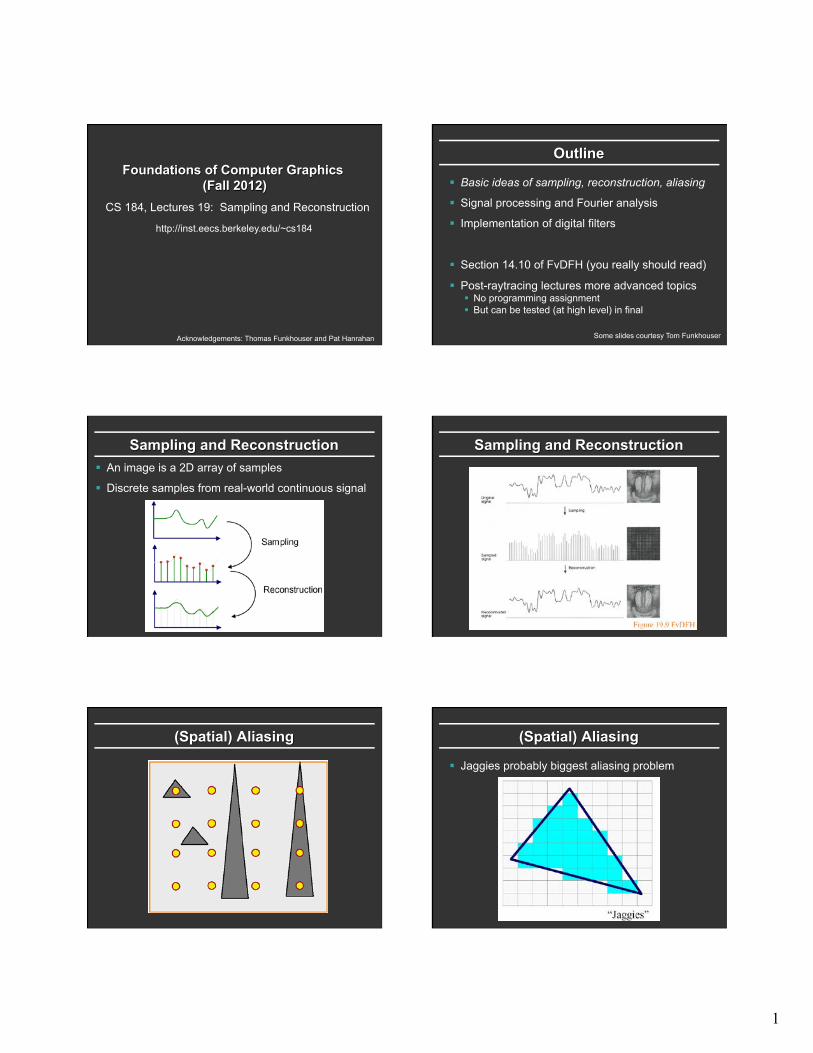
Sampling and Reconstruction §  An image is a 2D array of samples

§  Discrete samples from real-world continuous signal

Sampling and Reconstruction

(Spatial) Aliasing (Spatial) Aliasing

§  Jaggies probably biggest aliasing problem

2

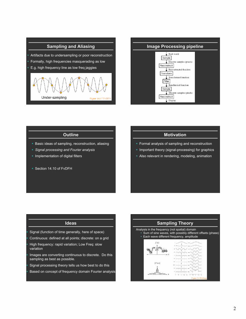
Sampling and Aliasing

§  Artifacts due to undersampling or poor reconstruction

§  Formally, high frequencies masquerading as low

§  E.g. high frequency line as low freq jaggies

Image Processing pipeline

Outline

§  Basic ideas of sampling, reconstruction, aliasing

§  Signal processing and Fourier analysis

§  Implementation of digital filters

§  Section 14.10 of FvDFH

Motivation

§  Formal analysis of sampling and reconstruction

§  Important theory (signal-processing) for graphics

§  Also relevant in rendering, modeling, animation

Ideas

§  Signal (function of time generally, here of space)

§  Continuous: defined at all points; discrete: on a grid

§  High frequency: rapid variation; Low Freq: slow variation

§  Images are converting continuous to discrete. Do this sampling as best as possible.

§  Signal processing theory tells us how best to do this

§  Based on concept of frequency domain Fourier analysis

Sampling Theory Analysis in the frequency (not spatial) domain

§  Sum of sine waves, with possibly different offsets (phase) §  Each wave different frequency, amplitude

3

Fourier Transform

§  Tool for converting from spatial to frequency domain

§  Or vice versa

§  One of most important mathematical ideas

§  Computational algorithm: Fast Fourier Transform §  One of 10 great algorithms scientific computing §  Makes Fourier processing possible (images etc.) §  Not discussed here, but look up if interested

Fourier Transform

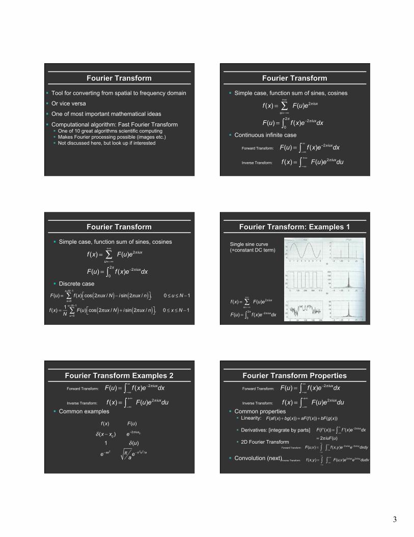
§  Simple case, function sum of sines, cosines

§  Continuous infinite case

f (x) =u=−∞

+∞

∑ F(u)e2π iux

F(u) = f (x)e−2π iux

0

2π

∫ dx

Forward Transform: F(u) = f (x)e−2π iux

−∞

∞

∫ dx

Inverse Transform: f (x) =−∞

+∞

∫ F(u)e2π iuxdu

Fourier Transform

§  Simple case, function sum of sines, cosines

§  Discrete case

f (x) =u=−∞

+∞

∑ F(u)e2π iux

F(u) = f (x)e−2π iux

0

2π

∫ dx

F(u) = f (x) cos 2πux / N( )− i sin 2πux / n( )⎡⎣ ⎤⎦x=0

x=N−1

∑ , 0 ≤ u ≤ N −1

f (x) = 1N

F(u) cos 2πux / N( ) + i sin 2πux / n( )⎡⎣ ⎤⎦u=0

u=N−1

∑ , 0 ≤ x ≤ N −1

Fourier Transform: Examples 1

f (x) =u=−∞

+∞

∑ F(u)e2π iux

F(u) = f (x)e−2π iux

0

2π

∫ dx

Single sine curve (+constant DC term)

Fourier Transform Examples 2

Forward Transform: F(u) = f (x)e−2π iux

−∞

∞

∫ dx

Inverse Transform: f (x) =−∞

+∞

∫ F(u)e2π iuxdu§  Common examples

δ (x − x0) e−2π iux0

1 δ (u)

e−ax2 πa

e−π 2u2 /a

f (x) F(u)

Fourier Transform Properties

Forward Transform: F(u) = f (x)e−2π iux

−∞

∞

∫ dx

Inverse Transform: f (x) =−∞

+∞

∫ F(u)e2π iuxdu§  Common properties

§  Linearity:

§  Derivatives: [integrate by parts]

§  2D Fourier Transform

§  Convolution (next)

F(f '(x)) = f '(x)e−2π iux

−∞

∞

∫ dx

= 2π iuF(u)

F(af (x)+ bg(x)) = aF(f (x))+ bF(g(x))

Forward Transform: F(u,v) =−∞

∞

∫ f (x,y)e−2π iux

−∞

∞

∫ e−2π ivydxdy

Inverse Transform: f (x,y) =−∞

∞

∫ −∞

+∞

∫ F(u,v)e2π iuxe2π ivydudv

4

Sampling Theorem, Bandlimiting §  A signal can be reconstructed from its samples,

if the original signal has no frequencies above half the sampling frequency – Shannon

§  The minimum sampling rate for a bandlimited function is called the Nyquist rate

Sampling Theorem, Bandlimiting

§  A signal can be reconstructed from its samples, if the original signal has no frequencies above half the sampling frequency – Shannon

§  The minimum sampling rate for a bandlimited function is called the Nyquist rate

§  A signal is bandlimited if the highest frequency is bounded. This frequency is called the bandwidth

§  In general, when we transform, we want to filter to bandlimit before sampling, to avoid aliasing

Antialiasing

§  Sample at higher rate §  Not always possible §  Real world: lines have infinitely high frequencies,

can’t sample at high enough resolution

§  Prefilter to bandlimit signal §  Low-pass filtering (blurring) §  Trade blurriness for aliasing

Ideal bandlimiting filter

§  Formal derivation is homework exercise

Outline

§  Basic ideas of sampling, reconstruction, aliasing

§  Signal processing and Fourier analysis §  Convolution

§  Implementation of digital filters

§  Section 14.10 of FvDFH

Convolution 1

5

Convolution 2 Convolution 3

Convolution 4 Convolution 5

Convolution in Frequency Domain

Forward Transform: F(u) = f (x)e−2π iux

−∞

∞

∫ dx

Inverse Transform: f (x) =−∞

+∞

∫ F(u)e2π iuxdu§  Convolution (f is signal ; g is filter [or vice versa])

§  Fourier analysis (frequency domain multiplication)

h(y) = f (x)g(y − x)dx =−∞

+∞

∫ g(x)f (y − x)dx−∞

+∞

∫h = f * g or f ⊗ g

H(u) = F(u)G(u)

Practical Image Processing §  Discrete convolution (in spatial domain) with filters for

various digital signal processing operations

§  Easy to analyze, understand effects in frequency domain §  E.g. blurring or bandlimiting by convolving with low pass filter

6

Outline

§  Basic ideas of sampling, reconstruction, aliasing

§  Signal processing and Fourier analysis

§  Implementation of digital filters

§  Section 14.10 of FvDFH

Discrete Convolution §  Previously: Convolution as mult in freq domain

§  But need to convert digital image to and from to use that §  Useful in some cases, but not for small filters

§  Previously seen: Sinc as ideal low-pass filter §  But has infinite spatial extent, exhibits spatial ringing §  In general, use frequency ideas, but consider

implementation issues as well

§  Instead, use simple discrete convolution filters e.g. §  Pixel gets sum of nearby pixels weighted by filter/mask

2 0 -7

5 4 9

1 -6 -2

Implementing Discrete Convolution §  Fill in each pixel new image convolving with old

§  Not really possible to implement it in place

§  More efficient for smaller kernels/filters f

§  Normalization §  If you don’t want overall brightness change, entries of filter

must sum to 1. You may need to normalize by dividing

§  Integer arithmetic §  Simpler and more efficient §  In general, normalization outside, round to nearest int

Inew (a,b) = f (x − a,y − b)Iold (x,y)

y=b−width

b+width

∑x=a−width

a+width

∑

Outline

§  Implementation of digital filters §  Discrete convolution in spatial domain §  Basic image-processing operations §  Antialiased shift and resize

Basic Image Processing

§  Blur

§  Sharpen

§  Edge Detection

All implemented using convolution with different filters

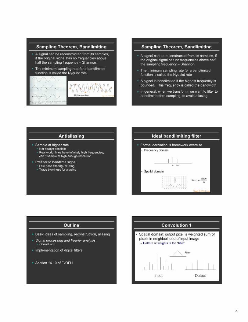
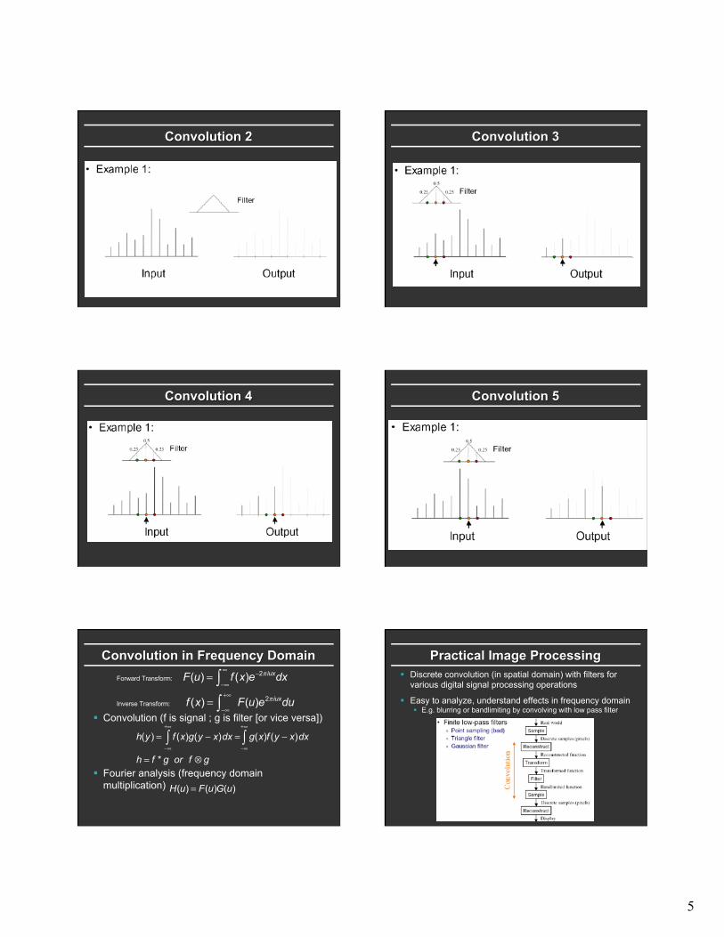
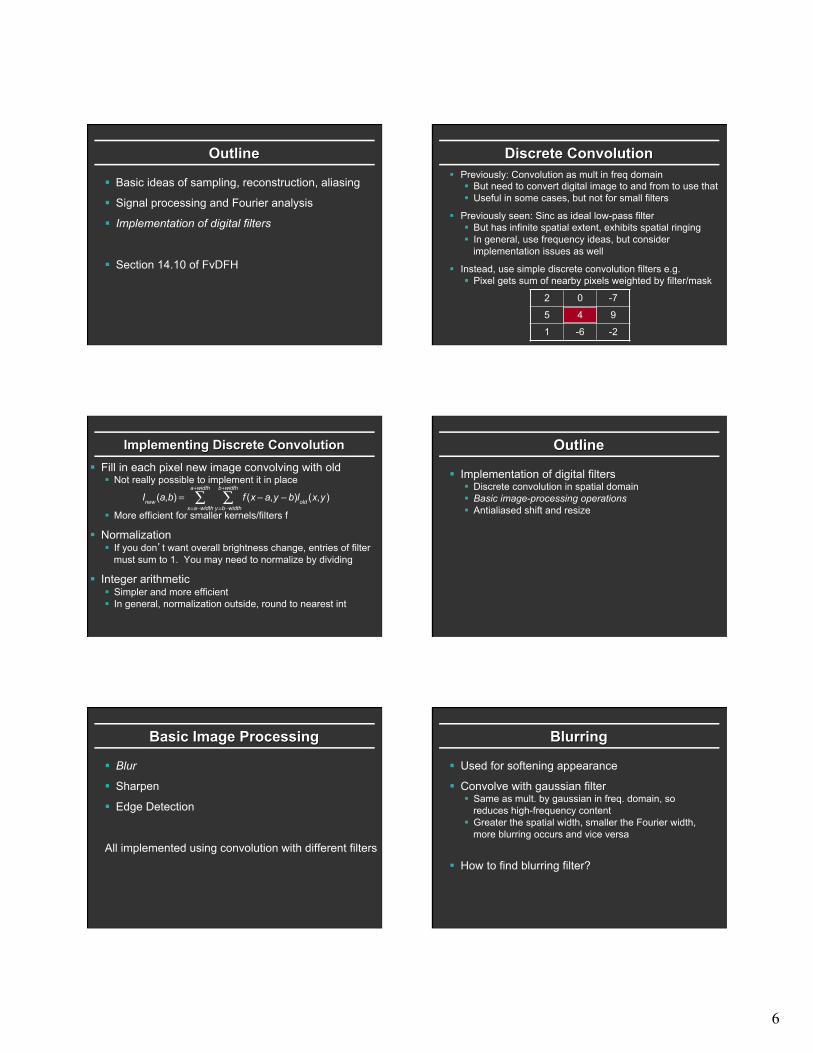
Blurring

§  Used for softening appearance

§  Convolve with gaussian filter §  Same as mult. by gaussian in freq. domain, so

reduces high-frequency content §  Greater the spatial width, smaller the Fourier width,

more blurring occurs and vice versa

§  How to find blurring filter?

7

Blurring Blurring

Blurring Blurring

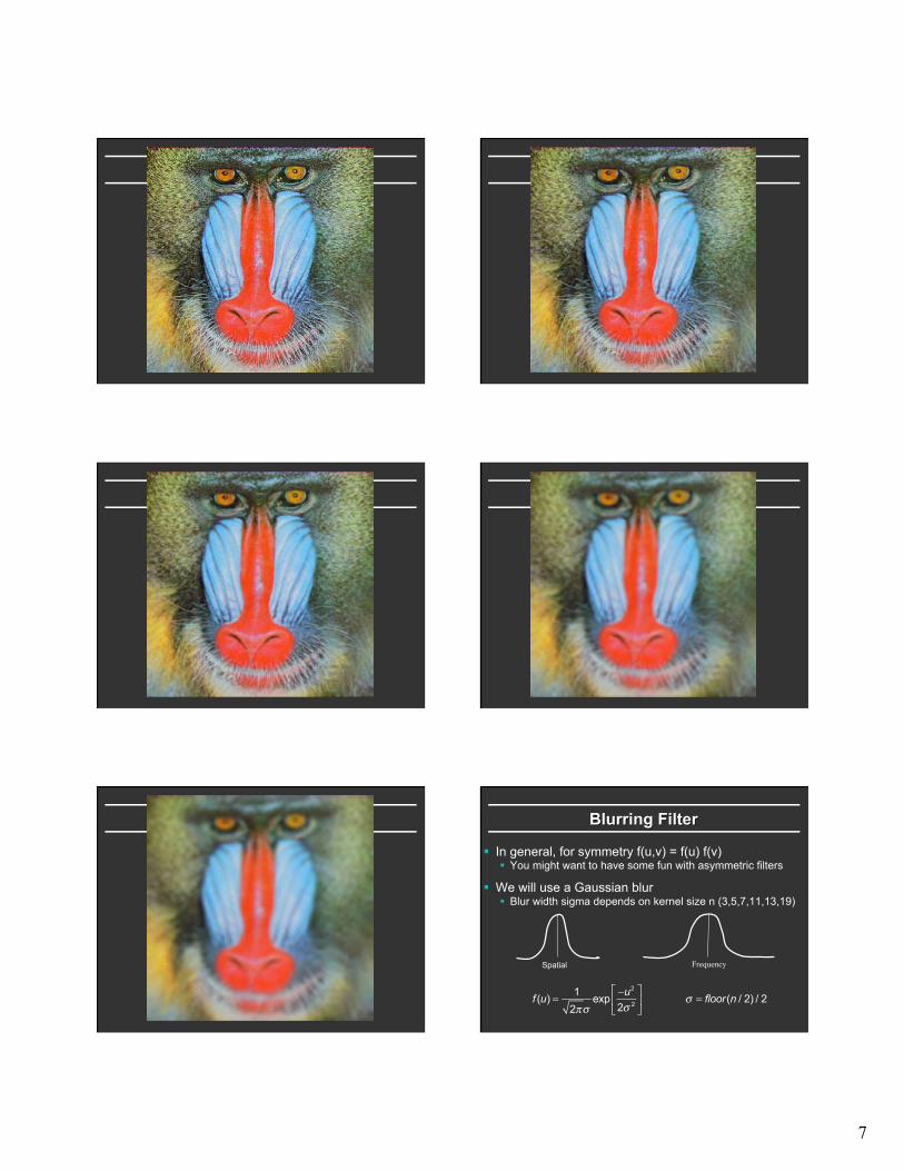
Blurring Blurring Filter

§  In general, for symmetry f(u,v) = f(u) f(v) §  You might want to have some fun with asymmetric filters

§  We will use a Gaussian blur §  Blur width sigma depends on kernel size n (3,5,7,11,13,19)

Spatial Frequency

f (u) = 1

2πσexp

−u2

2σ 2

⎡

⎣⎢

⎤

⎦⎥ σ = floor(n / 2) / 2

8

Discrete Filtering, Normalization

§  Gaussian is infinite §  In practice, finite filter of size n (much less energy beyond 2

sigma or 3 sigma). §  Must renormalize so entries add up to 1

§  Simple practical approach §  Take smallest values as 1 to scale others, round to integers §  Normalize. E.g. for n = 3, sigma = ½

f (u,v) = 1

2πσ 2 exp − u2 +v 2

2σ 2

⎡

⎣⎢

⎤

⎦⎥ =

2π

exp −2 u2 +v 2( )⎡⎣

⎤⎦

≈0.012 0.09 0.0120.09 0.64 0.090.012 0.09 0.012

⎛

⎝

⎜⎜

⎞

⎠

⎟⎟ ≈

186

1 7 17 54 71 7 1

⎛

⎝

⎜⎜

⎞

⎠

⎟⎟

Basic Image Processing

§  Blur

§  Sharpen

§  Edge Detection

All implemented using convolution with different filters

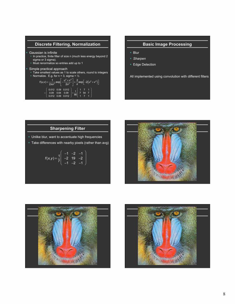
Sharpening Filter

§  Unlike blur, want to accentuate high frequencies

§  Take differences with nearby pixels (rather than avg)

f (x,y) = 17

−1 −2 −1−2 19 −2−1 −2 −1

⎛

⎝

⎜⎜

⎞

⎠

⎟⎟

Blurring

Blurring Blurring

9

Basic Image Processing

§  Blur

§  Sharpen

§  Edge Detection

All implemented using convolution with different filters

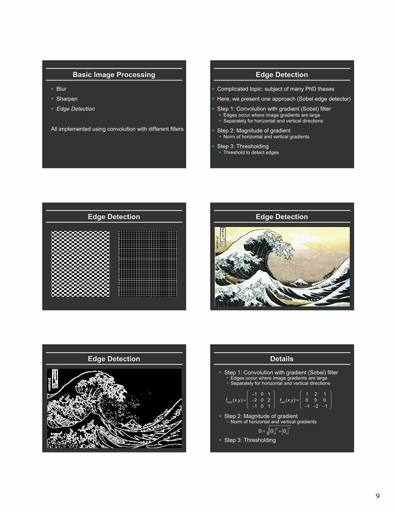
Edge Detection

§  Complicated topic: subject of many PhD theses

§  Here, we present one approach (Sobel edge detector)

§  Step 1: Convolution with gradient (Sobel) filter §  Edges occur where image gradients are large §  Separately for horizontal and vertical directions

§  Step 2: Magnitude of gradient §  Norm of horizontal and vertical gradients

§  Step 3: Thresholding §  Threshold to detect edges

Edge Detection Edge Detection

Edge Detection Details

§  Step 1: Convolution with gradient (Sobel) filter §  Edges occur where image gradients are large §  Separately for horizontal and vertical directions

§  Step 2: Magnitude of gradient §  Norm of horizontal and vertical gradients

§  Step 3: Thresholding

fhoriz(x,y) =−1 0 1−2 0 2−1 0 1

⎛

⎝

⎜⎜

⎞

⎠

⎟⎟ fvert (x,y) =

1 2 10 0 0−1 −2 −1

⎛

⎝

⎜⎜

⎞

⎠

⎟⎟

G = Gx

2+ Gy

2

10

Outline

§  Implementation of digital filters §  Discrete convolution in spatial domain §  Basic image-processing operations §  Antialiased shift and resize

Antialiased Shift

Shift image based on (fractional) sx and sy §  Check for integers, treat separately §  Otherwise convolve/resample with kernel/filter h:

u = x − sx v = y − sy

I(x,y) = h(u '− u,v '−v)I(u ',v ')

u ',v '∑

Antialiased Scale Magnification

Magnify image (scale s or γ > 1) §  Interpolate between orig. samples to evaluate frac vals §  Do so by convolving/resampling with kernel/filter: §  Treat the two image dimensions independently (diff scales)

u = x

γ

I(x) = h(u '− u)I(u ')

u '=u/γ −width

u/γ +width

∑

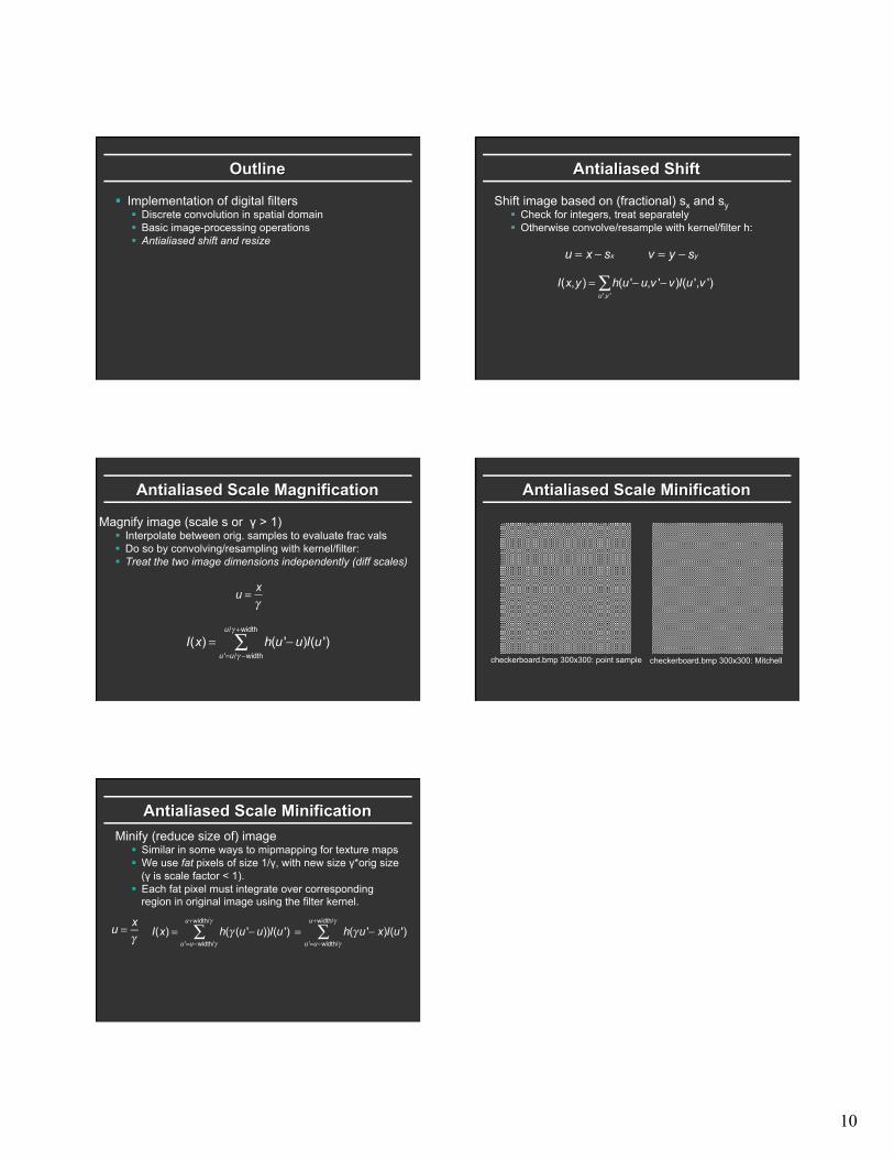
Antialiased Scale Minification

checkerboard.bmp 300x300: point sample checkerboard.bmp 300x300: Mitchell

Antialiased Scale Minification Minify (reduce size of) image

§  Similar in some ways to mipmapping for texture maps §  We use fat pixels of size 1/γ, with new size γ*orig size

(γ is scale factor < 1). §  Each fat pixel must integrate over corresponding

region in original image using the filter kernel.

u = x

γ I(x) = h(γ (u '− u))I(u ')

u '=u−width/γ

u+width/γ

∑ = h(γ u '− x)I(u ')u '=u−width/γ

u+width/γ

∑