Sampling & Quantization

by Erol Seke

For the course “Communications”

ESKİŞEHİR OSMANGAZİ UNIVERSITY

General Communication System

ADC

DAC

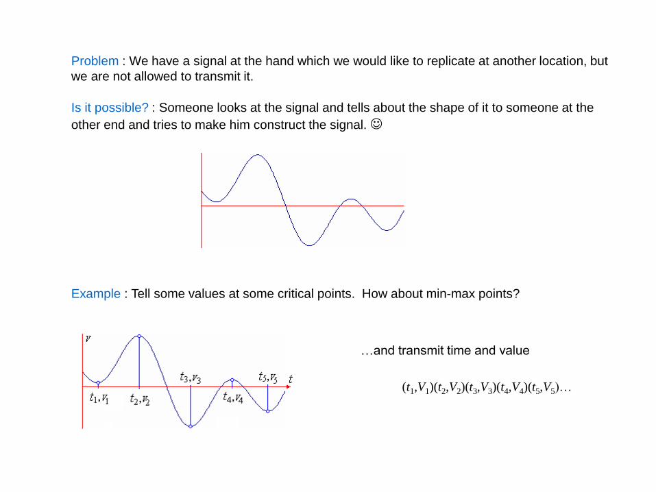
Problem : We have a signal at the hand which we would like to replicate at another location, but

we are not allowed to transmit it.

Is it possible? : Someone looks at the signal and tells about the shape of it to someone at the

other end and tries to make him construct the signal.

Example : Tell some values at some critical points. How about min-max points?

(t1,V1)(t2,V2)(t3,V3)(t4,V4)(t5,V5)…

…and transmit time and value

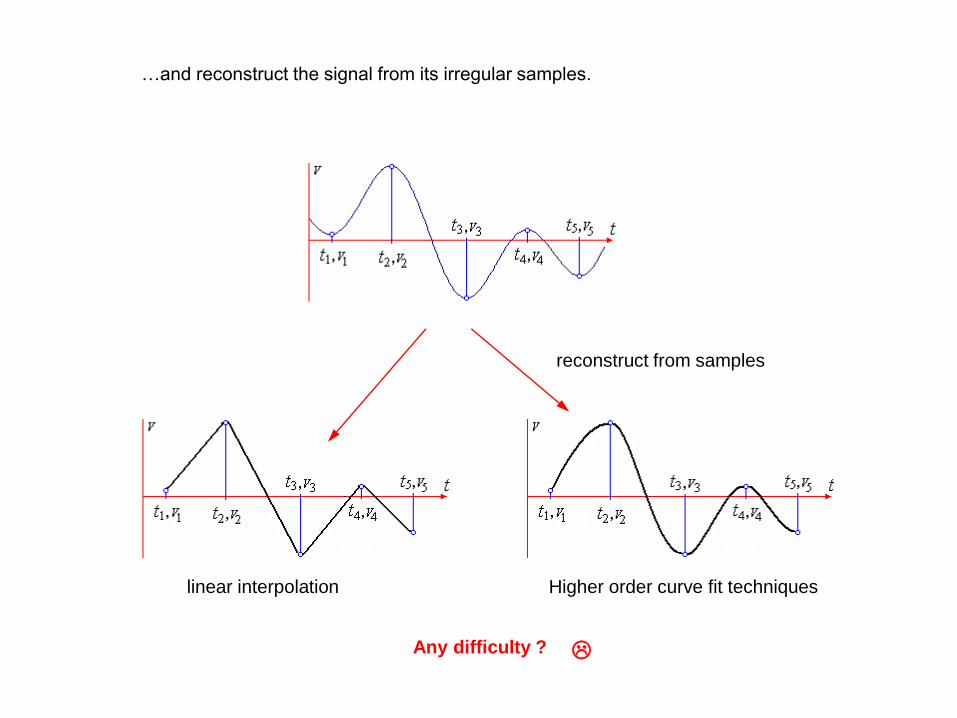
reconstruct from samples

…and reconstruct the signal from its irregular samples.

linear interpolation Higher order curve fit techniques

Any difficulty ?

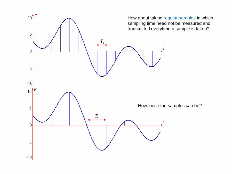
How about taking regular samples in which

sampling time need not be measured and

transmitted everytime a sample is taken?

How loose the samples can be?

Ts

Ts

Nyquist’s sampling criterion : A baseband signal with the highest frequency component at fm

can be reconstructed from its samples if the interval between samples is less than 1/2fm

That is; sampling frequency must be higher than twice the highest frequency of the signal

n

n

sms nTtfnTxtx ))(2sinc()()(

The sum of all sincs

reconstruction formula

a special case when

m

sf

T2

1

truncated sinc function

x[n]

n

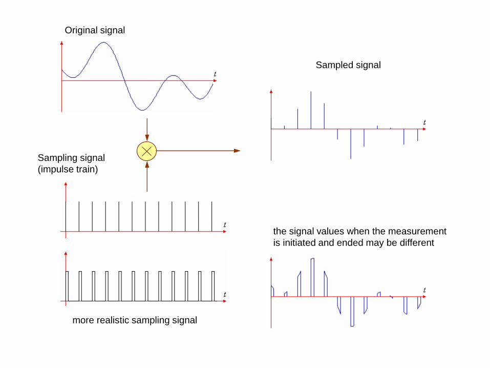
Original signal

Sampling signal

(impulse train)

Sampled signal

more realistic sampling signal

the signal values when the measurement

is initiated and ended may be different

t……

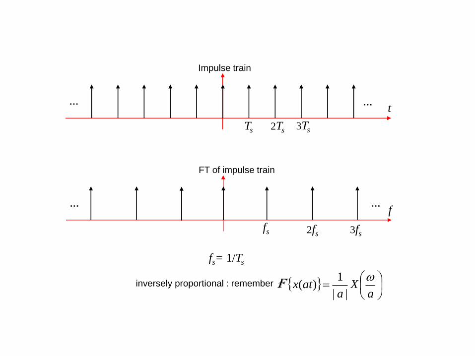
Impulse train

Ts 2Ts 3Ts

f……

FT of impulse train

fs 2fs 3fs

fs= 1/Ts

inversely proportional : remember

aX

aatx

||

1)(F

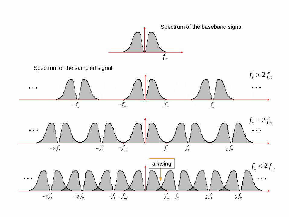
Spectrum of the baseband signal

Spectrum of the sampled signal

ms ff 2

ms ff 2

ms ff 2aliasing

mf

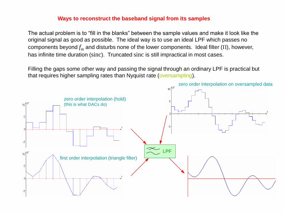
Ways to reconstruct the baseband signal from its samples

The actual problem is to “fill in the blanks” between the sample values and make it look like the

original signal as good as possible. The ideal way is to use an ideal LPF which passes no

components beyond fm and disturbs none of the lower components. Ideal filter (Π), however,

has infinite time duration (sinc). Truncated sinc is still impractical in most cases.

Filling the gaps some other way and passing the signal through an ordinary LPF is practical but

that requires higher sampling rates than Nyquist rate (oversampling).

zero order interpolation (hold)(this is what DACs do)

first order interpolation (triangle filter)

LPF

zero order interpolation on oversampled data

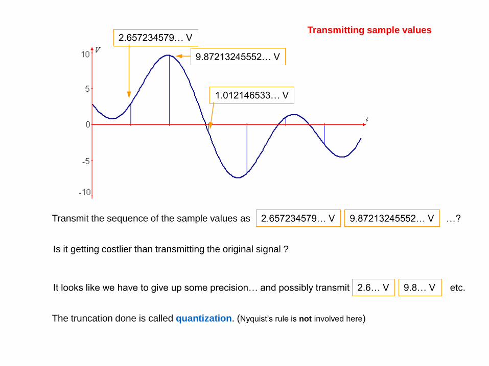
2.657234579… V

9.87213245552… V

1.012146533… V

Transmit the sequence of the sample values as 2.657234579… V 9.87213245552… V …?

Is it getting costlier than transmitting the original signal ?

It looks like we have to give up some precision… and possibly transmit 2.6… V 9.8… V etc.

The truncation done is called quantization. (Nyquist’s rule is not involved here)

Transmitting sample values

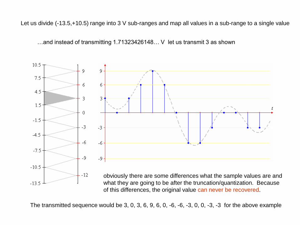
Let us divide (-13.5,+10.5) range into 3 V sub-ranges and map all values in a sub-range to a single value

…and instead of transmitting 1.71323426148… V let us transmit 3 as shown

obviously there are some differences what the sample values are and

what they are going to be after the truncation/quantization. Because

of this differences, the original value can never be recovered.

The transmitted sequence would be 3, 0, 3, 6, 9, 6, 0, -6, -6, -3, 0, 0, -3, -3 for the above example

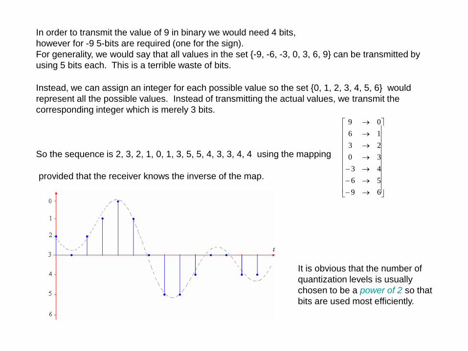
In order to transmit the value of 9 in binary we would need 4 bits,

however for -9 5-bits are required (one for the sign).

For generality, we would say that all values in the set {-9, -6, -3, 0, 3, 6, 9} can be transmitted by

using 5 bits each. This is a terrible waste of bits.

Instead, we can assign an integer for each possible value so the set {0, 1, 2, 3, 4, 5, 6} would

represent all the possible values. Instead of transmitting the actual values, we transmit the

corresponding integer which is merely 3 bits.

So the sequence is 2, 3, 2, 1, 0, 1, 3, 5, 5, 4, 3, 3, 4, 4 using the mapping

69

56

43

30

23

16

09

provided that the receiver knows the inverse of the map.

It is obvious that the number of

quantization levels is usually

chosen to be a power of 2 so that

bits are used most efficiently.

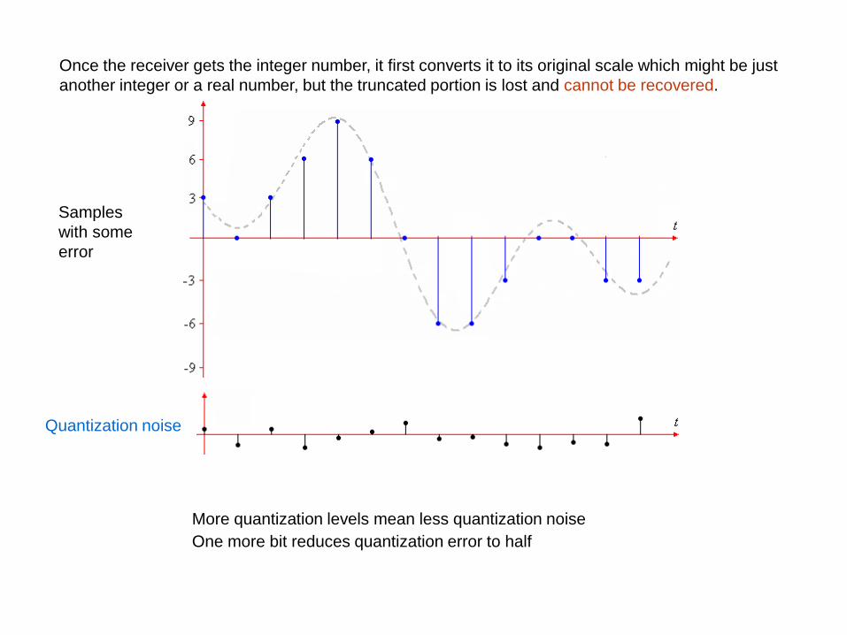
Once the receiver gets the integer number, it first converts it to its original scale which might be just

another integer or a real number, but the truncated portion is lost and cannot be recovered.

Quantization noise

Samples

with some

error

More quantization levels mean less quantization noise

One more bit reduces quantization error to half

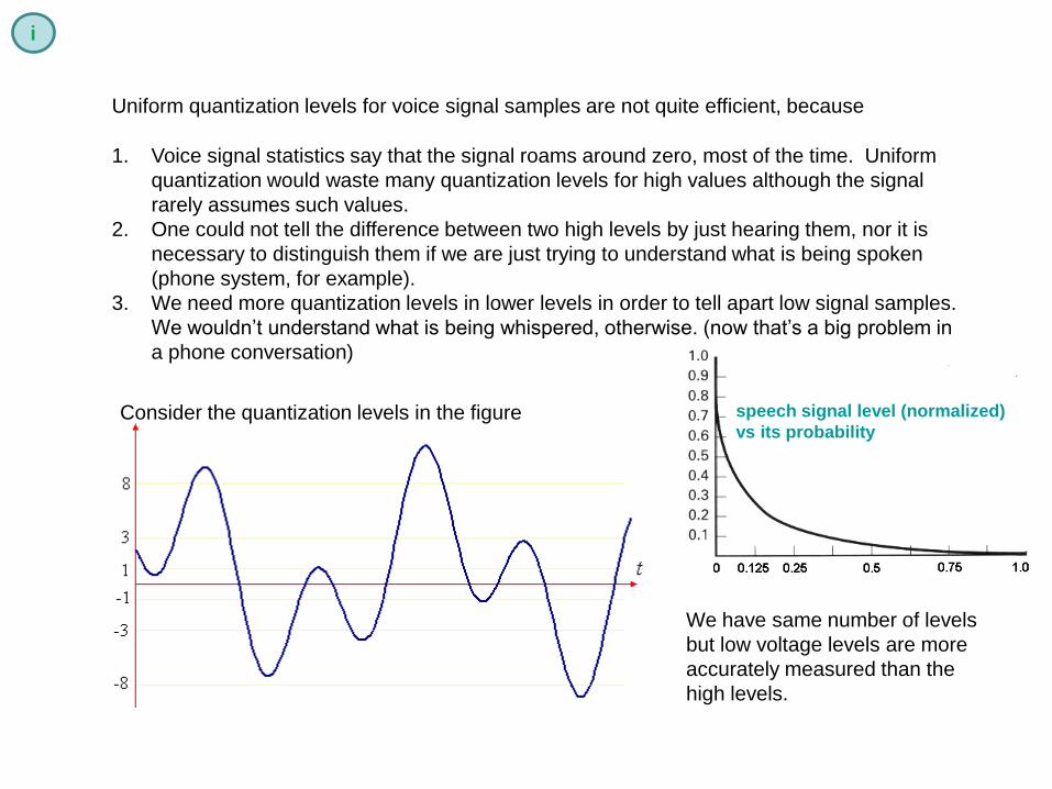
Uniform quantization levels for voice signal samples are not quite efficient, because

1. Voice signal statistics say that the signal roams around zero, most of the time. Uniform

quantization would waste many quantization levels for high values although the signal

rarely assumes such values.

2. One could not tell the difference between two high levels by just hearing them, nor it is

necessary to distinguish them if we are just trying to understand what is being spoken

(phone system, for example).

3. We need more quantization levels in lower levels in order to tell apart low signal samples.

We wouldn’t understand what is being whispered, otherwise. (now that’s a big problem in

a phone conversation)

Consider the quantization levels in the figure

We have same number of levels

but low voltage levels are more

accurately measured than the

high levels.

speech signal level (normalized)

vs its probability

i

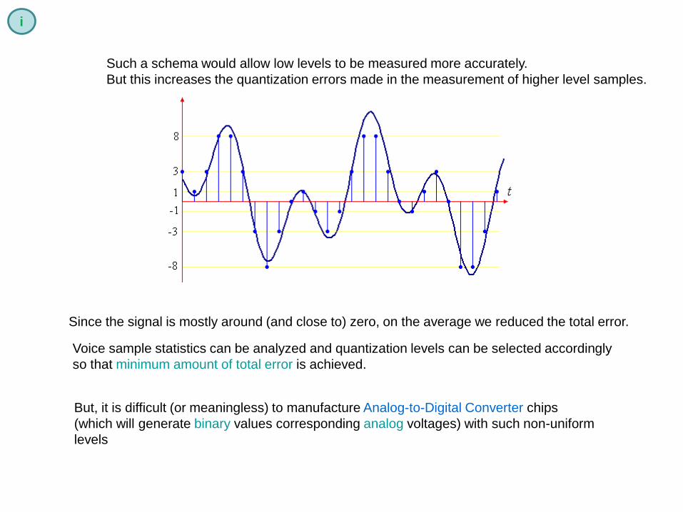
Such a schema would allow low levels to be measured more accurately.

But this increases the quantization errors made in the measurement of higher level samples.

Since the signal is mostly around (and close to) zero, on the average we reduced the total error.

Voice sample statistics can be analyzed and quantization levels can be selected accordingly

so that minimum amount of total error is achieved.

But, it is difficult (or meaningless) to manufacture Analog-to-Digital Converter chips

(which will generate binary values corresponding analog voltages) with such non-uniform

levels

i

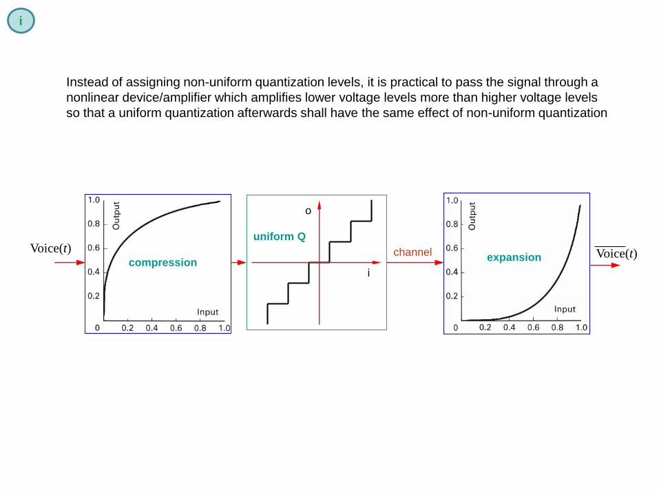
Instead of assigning non-uniform quantization levels, it is practical to pass the signal through a

nonlinear device/amplifier which amplifies lower voltage levels more than higher voltage levels

so that a uniform quantization afterwards shall have the same effect of non-uniform quantization

compressionexpansion

Voice(t)

i

o

uniform Q

channel Voice(t)

i

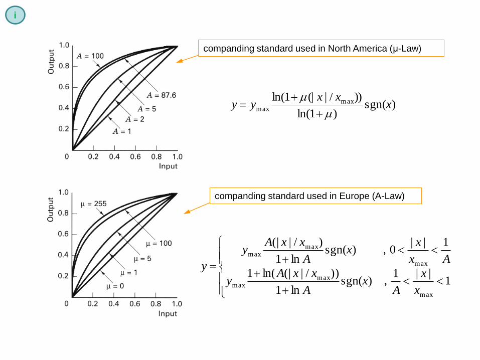
companding standard used in North America (μ-Law)

companding standard used in Europe (A-Law)

1||1

,)sgn(ln1

))/|(|ln(1

1||0,)sgn(

ln1

)/|(|

max

maxmax

max

maxmax

x

x

Ax

A

xxAy

Ax

xx

A

xxAy

y

)sgn()1ln(

))/|(|1ln( maxmax x

xxyy

i

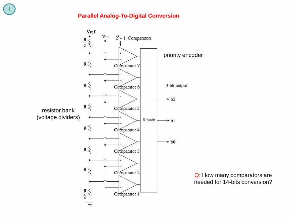
Parallel Analog-To-Digital Conversion

resistor bank

(voltage dividers)

priority encoder

Q: How many comparators are

needed for 14-bits conversion?

i

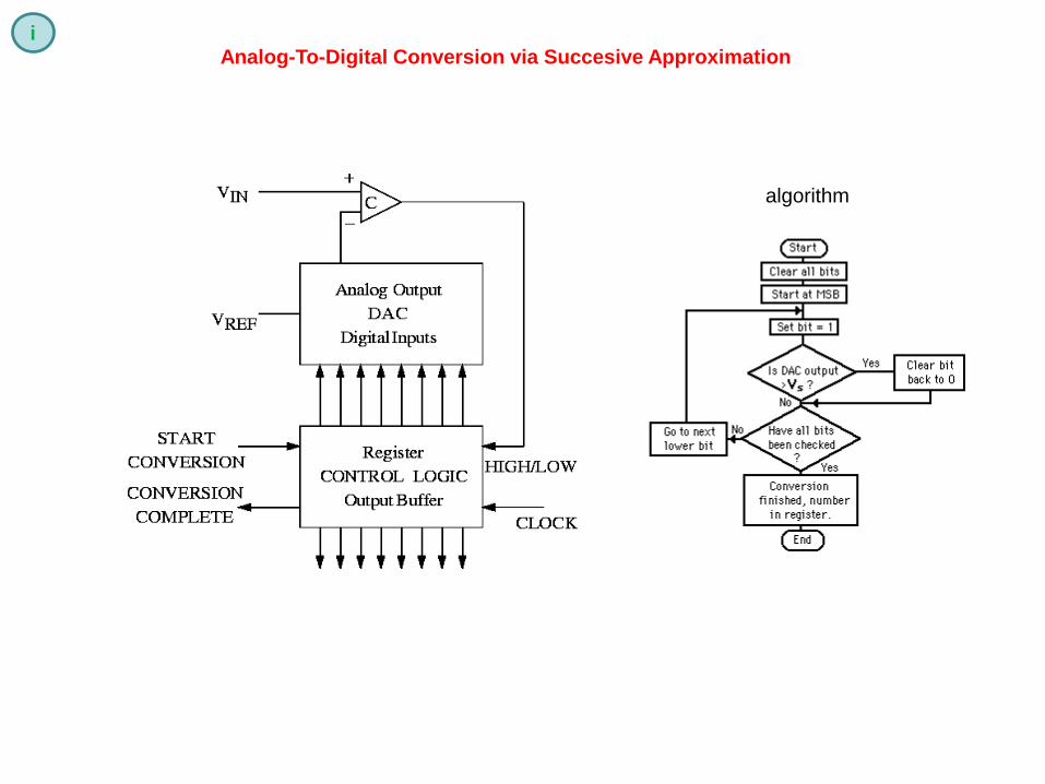
Analog-To-Digital Conversion via Succesive Approximation

algorithm

i

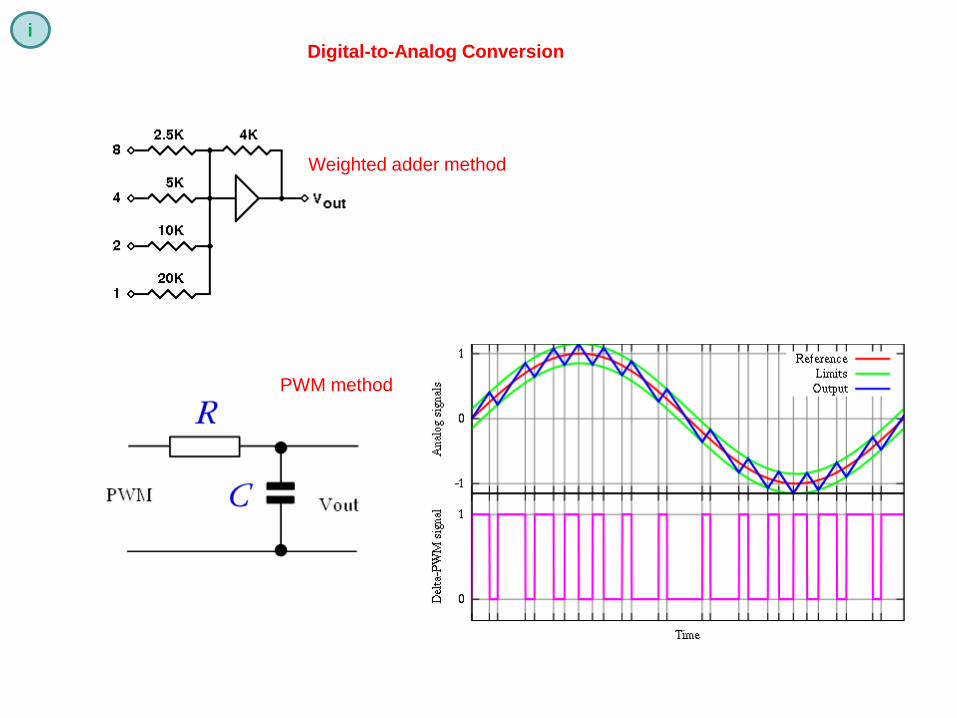
Digital-to-Analog Conversion

Weighted adder method

PWM method

i

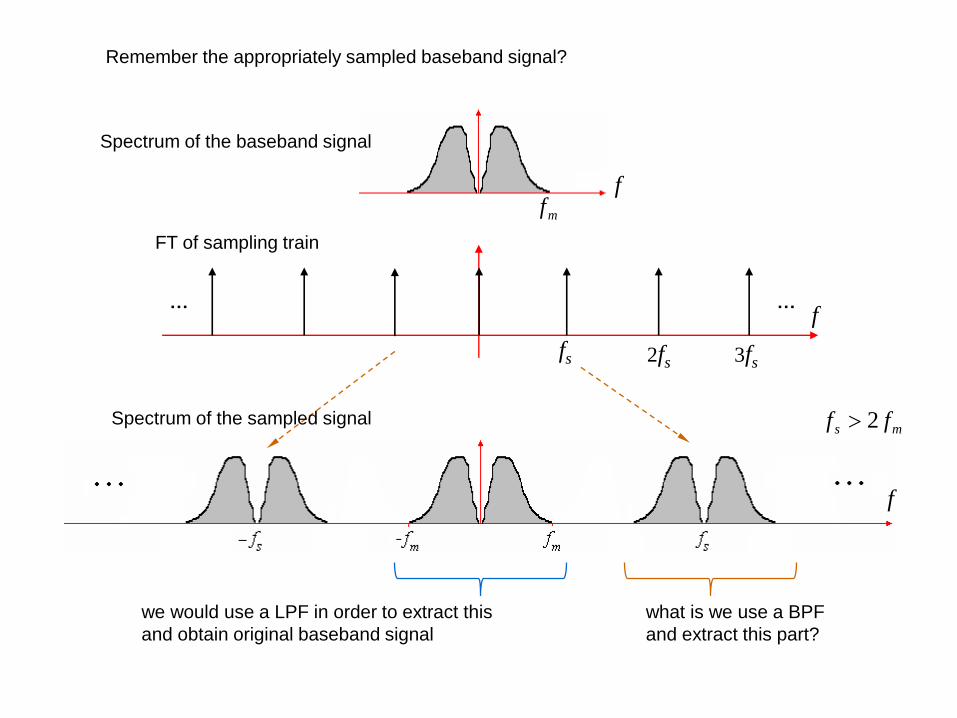
Spectrum of the baseband signal

ms ff 2

mf

Remember the appropriately sampled baseband signal?

f……

FT of sampling train

fs 2fs 3fs

f

f

Spectrum of the sampled signal

we would use a LPF in order to extract this

and obtain original baseband signal

what is we use a BPF

and extract this part?

| ( ) |X f

f

| ( ) |S f

f

sf skf0

B

f

| ( ) |XS f

B

sf

sf skf0sf

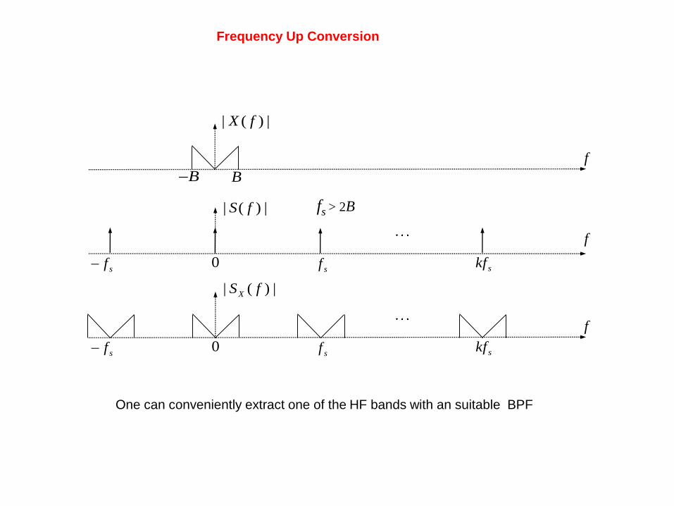
Frequency Up Conversion

One can conveniently extract one of the HF bands with an suitable BPF

fs > 2B

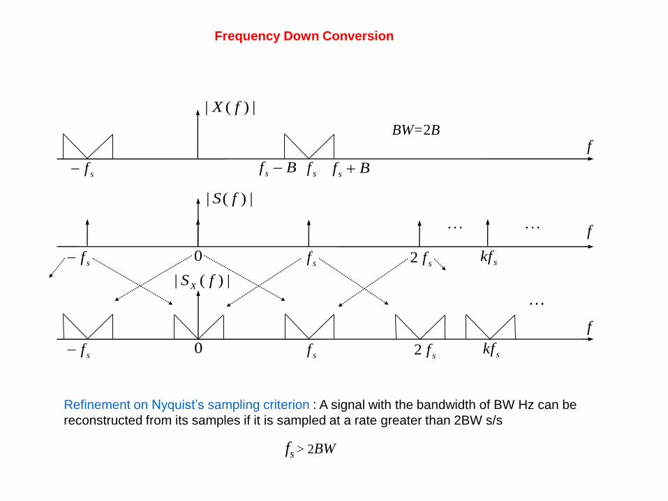
Frequency Down Conversion

| ( ) |X f

f

| ( ) |S f

f

sf skf0

f

| ( ) |XS f

sf

sf skf0sf

sfsf sf Bsf B

2 sf

2 sf

Refinement on Nyquist’s sampling criterion : A signal with the bandwidth of BW Hz can be

reconstructed from its samples if it is sampled at a rate greater than 2BW s/s

fs > 2BW

BW=2B

| ( ) |X f

f

| ( ) |S f

f

sf skf0

f

| ( ) |XS f

sf

sf skf0sf

sfsf sf B

2 sf

2 sf

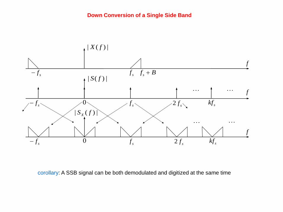
Down Conversion of a Single Side Band

corollary: A SSB signal can be both demodulated and digitized at the same time

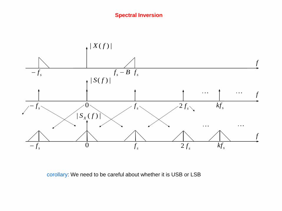
Spectral Inversion

| ( ) |X f

f

| ( ) |S f

f

sf skf0

f

| ( ) |XS f

sf

sf skf0sf

sfsf sf B

2 sf

2 sf

corollary: We need to be careful about whether it is USB or LSB

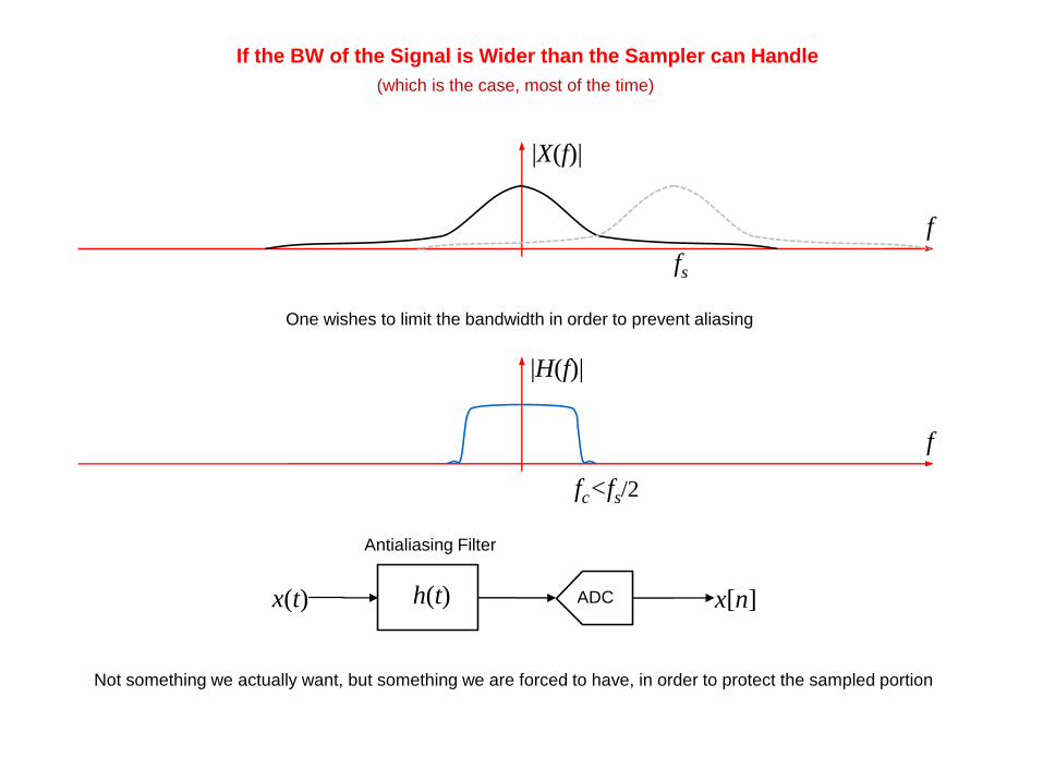
If the BW of the Signal is Wider than the Sampler can Handle

f

fs

|X(f)|

(which is the case, most of the time)

One wishes to limit the bandwidth in order to prevent aliasing

f

fc<fs/2

|H(f)|

x(t) h(t) ADC x[n]

Antialiasing Filter

Not something we actually want, but something we are forced to have, in order to protect the sampled portion

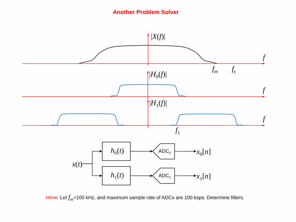
f

|X(f)|

f

|H0(f)|

f

|H1(f)|

f1

x(t)

h0(t) ADC0 x0[n]

h1(t) ADC1 x1[n]

fm

Another Problem Solver

Hmw: Let fm=100 kHz, and maximum sample rate of ADCs are 100 ksps. Determine filters.

fs

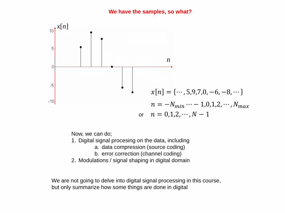
We have the samples, so what?

Now, we can do;

1. Digital signal procesing on the data, including

a. data compression (source coding)

b. error correction (channel coding)

2. Modulations / signal shaping in digital domain

x[n]

n

𝑥 𝑛 = ⋯ , 5,9,7,0, −6, −8,⋯

𝑛 = −𝑁𝑚𝑖𝑛⋯− 1,0,1,2,⋯ ,𝑁𝑚𝑎𝑥

𝑛 = 0,1,2,⋯ ,𝑁 − 1or

We are not going to delve into digital signal processing in this course,

but only summarize how some things are done in digital

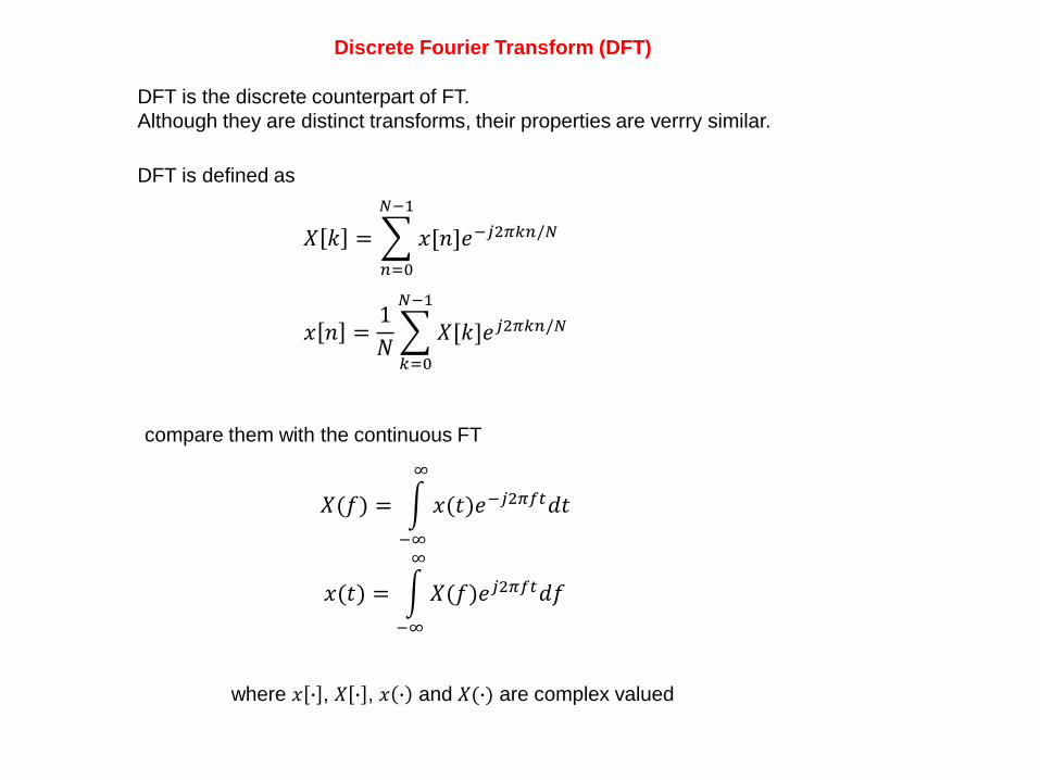
Discrete Fourier Transform (DFT)

DFT is the discrete counterpart of FT.

Although they are distinct transforms, their properties are verrry similar.

𝑋 𝑘 =

𝑛=0

𝑁−1

𝑥[𝑛]𝑒−𝑗2𝜋𝑘𝑛/𝑁

𝑥 𝑛 =1

𝑁

𝑘=0

𝑁−1

𝑋[𝑘]𝑒𝑗2𝜋𝑘𝑛/𝑁

𝑋(𝑓) = න

−∞

∞

𝑥(𝑡)𝑒−𝑗2𝜋𝑓𝑡𝑑𝑡

𝑥(𝑡) = න

−∞

∞

𝑋(𝑓)𝑒𝑗2𝜋𝑓𝑡𝑑𝑓

DFT is defined as

where 𝑥 ∙ , 𝑋 ∙ , 𝑥 ∙ and 𝑋(∙) are complex valued

compare them with the continuous FT

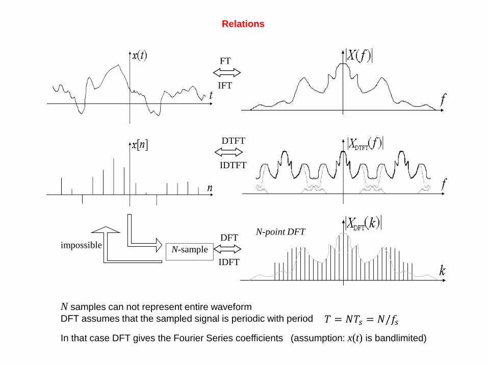
FT

IFT

N-sample

N-point DFT

impossible

DTFT

IDTFT

DFT

IDFT

N samples can not represent entire waveform

DFT assumes that the sampled signal is periodic with period

Relations

𝑇 = 𝑁𝑇𝑠 = 𝑁/𝑓𝑠

In that case DFT gives the Fourier Series coefficients (assumption: x(t) is bandlimited)

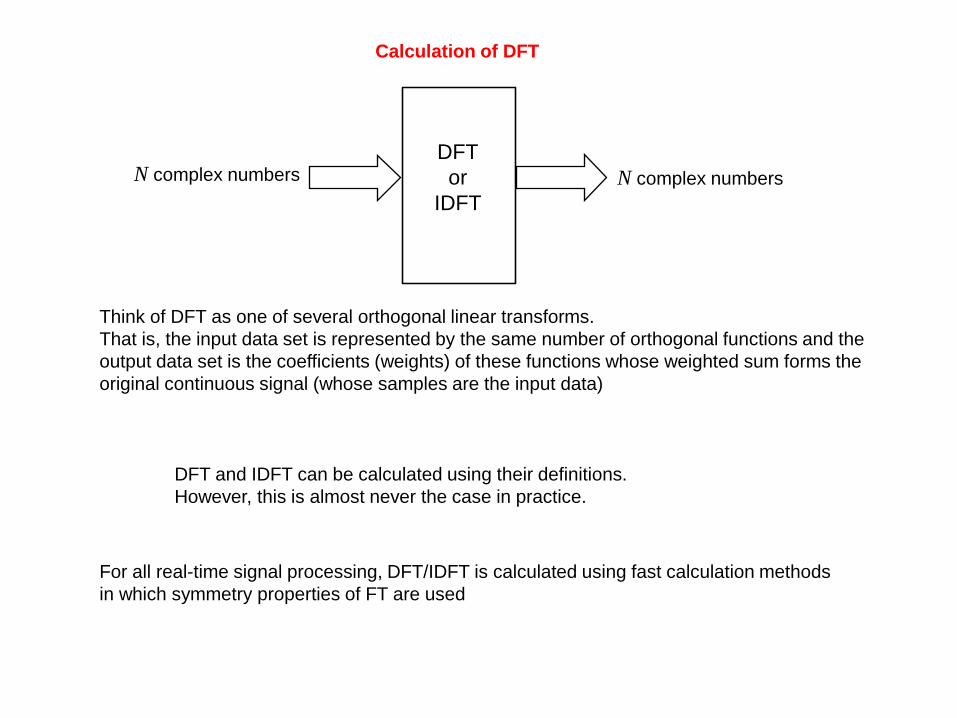
Calculation of DFT

DFT and IDFT can be calculated using their definitions.

However, this is almost never the case in practice.

N complex numbers N complex numbers

DFT

or

IDFT

For all real-time signal processing, DFT/IDFT is calculated using fast calculation methods

in which symmetry properties of FT are used

Think of DFT as one of several orthogonal linear transforms.

That is, the input data set is represented by the same number of orthogonal functions and the

output data set is the coefficients (weights) of these functions whose weighted sum forms the

original continuous signal (whose samples are the input data)

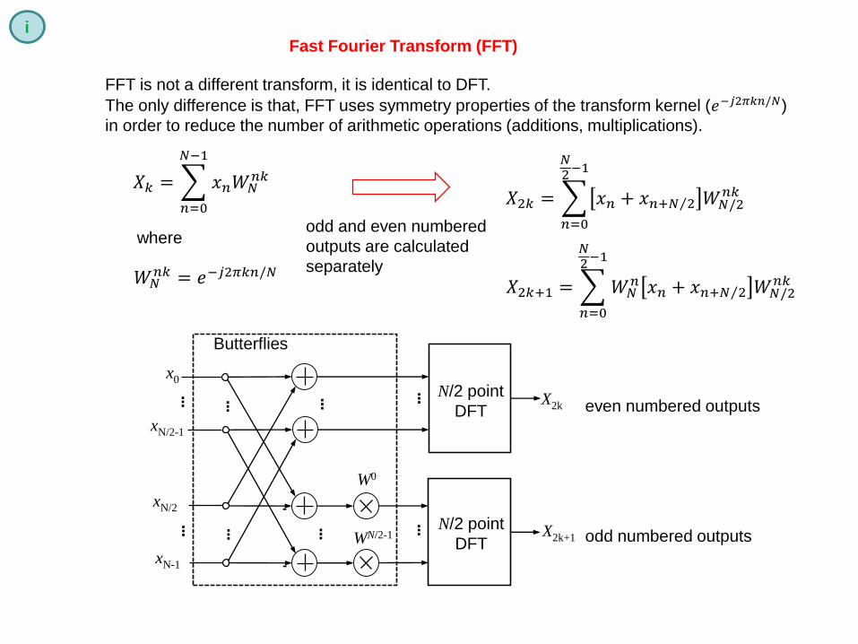
Fast Fourier Transform (FFT)

FFT is not a different transform, it is identical to DFT.

The only difference is that, FFT uses symmetry properties of the transform kernel (𝑒−𝑗2𝜋𝑘𝑛/𝑁)

in order to reduce the number of arithmetic operations (additions, multiplications).

odd numbered outputs

x0

xN/2

N/2 point

DFT

N/2 point

DFT

W0

X2k

X2k+1

-

Butterflies

xN/2-1

xN-1

WN/2-1

-

......

......

.........

... even numbered outputs

𝑋2𝑘 =

𝑛=0

𝑁2−1

𝑥𝑛 + 𝑥𝑛+ Τ𝑁 2 𝑊𝑁/2𝑛𝑘

𝑋2𝑘+1 =

𝑛=0

𝑁2−1

𝑊𝑁𝑛 𝑥𝑛 + 𝑥𝑛+ Τ𝑁 2 𝑊𝑁/2

𝑛𝑘𝑊𝑁𝑛𝑘 = 𝑒−𝑗2𝜋𝑘𝑛/𝑁

𝑋𝑘 =

𝑛=0

𝑁−1

𝑥𝑛𝑊𝑁𝑛𝑘

whereodd and even numbered

outputs are calculated

separately

i

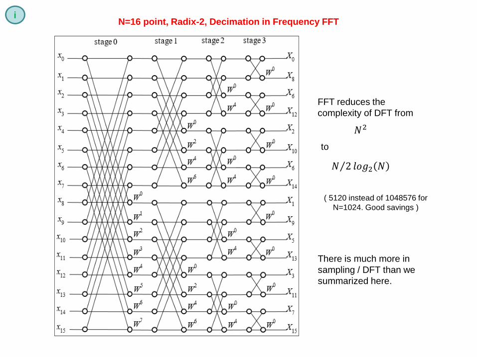
N=16 point, Radix-2, Decimation in Frequency FFT i

FFT reduces the

complexity of DFT from

)Τ𝑁 2 𝑙𝑜𝑔2(𝑁

𝑁2

to

( 5120 instead of 1048576 for

N=1024. Good savings )

There is much more in

sampling / DFT than we

summarized here.

Summary

1. What happens when we sample a continuous signal

2. Requirements for reconstructing the sampled signal

3. Frequency UpConversion / DownConversion while sampling / reconstruction

4. Relations between FS, FT, DFT, FFT

END