Embed Size (px)
DESCRIPTION
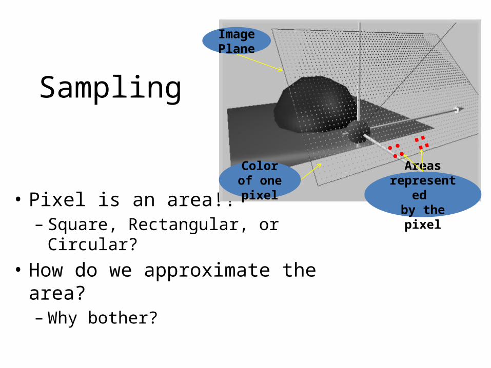
Sampling. Image Plane. Pixel is an area!! Square, Rectangular, or Circular? How do we approximate the area? Why bother?. Color of one pixel. Areas represented by the pixel. Alaising. Geometric Alias. Texture/Shading Alias. Shadow Alaising. More Subtle Alaising. - PowerPoint PPT Presentation
Citation preview
Sampling
• Pixel is an area!!– Square, Rectangular, or Circular?
• How do we approximate the area?– Why bother?
Color of one pixel
Image Plane
Areas represented by the pixel

AlaisingGeometric
Alias
Texture/Shading Alias

Shadow Alaising

More Subtle Alaising Should NOT see pattern!!
Maya Scene
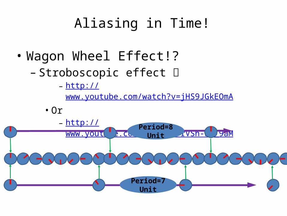
Aliasing in Time!
• Wagon Wheel Effect!?– Stroboscopic effect
– http://www.youtube.com/watch?v=jHS9JGkEOmA
• Or– http://www.youtube.com/watch?v=rVSh-au_9aM
Period=8 Unit
Period=7 Unit

Time/Space AnalogyColor “changes”
rapidly over space
Color “changes”slowly over space
• Many pixels to describe simple (no) transition
• In time, object moves very slowly, many frames to capture movement
• One pixel must capture many blackwhite transitions!
• One frame must capture much movement over time
• Observation: Aliasing results when …– Changes too fast for the sampling rates!

Intensity of the line
How to measure: rate of change?• Rate of Change:– Frequency!
• Frequency of images– How to measure?
• Goal:– Appreciation for
Nyquist frequency
One line of color

A little math …
• Approach:– Find mathematic representation for this simple case– Study to understand the characteristic– Generalize to discuss aliasing we observed
Assume width of 4 (T=4) Let’s say repeats every
width of 20 (W = 2*/10)
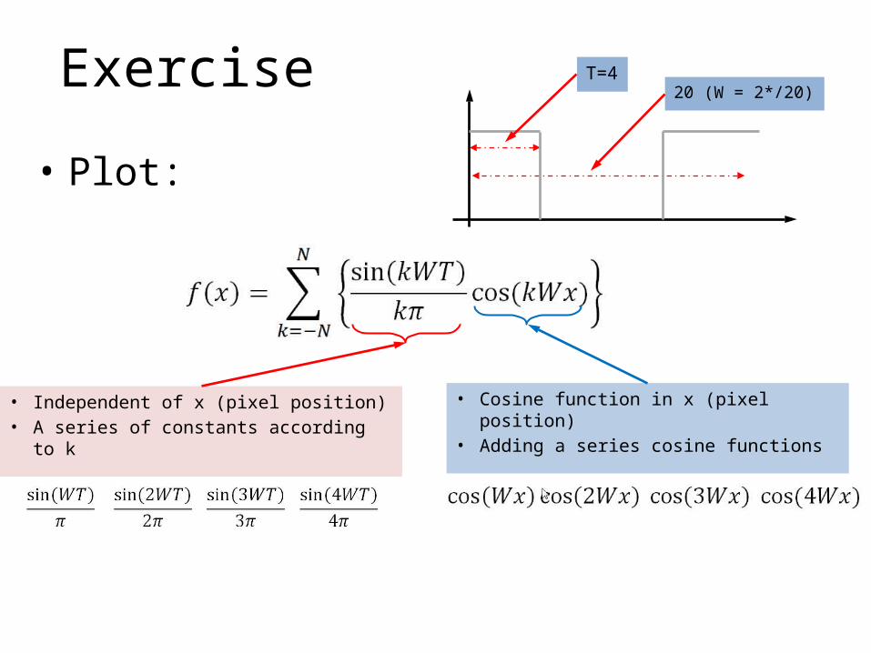
Exercise
• Plot:
T=420 (W = 2*/20)
• Independent of x (pixel position)• A series of constants according to k
• Cosine function in x (pixel position)• Adding a series cosine functions

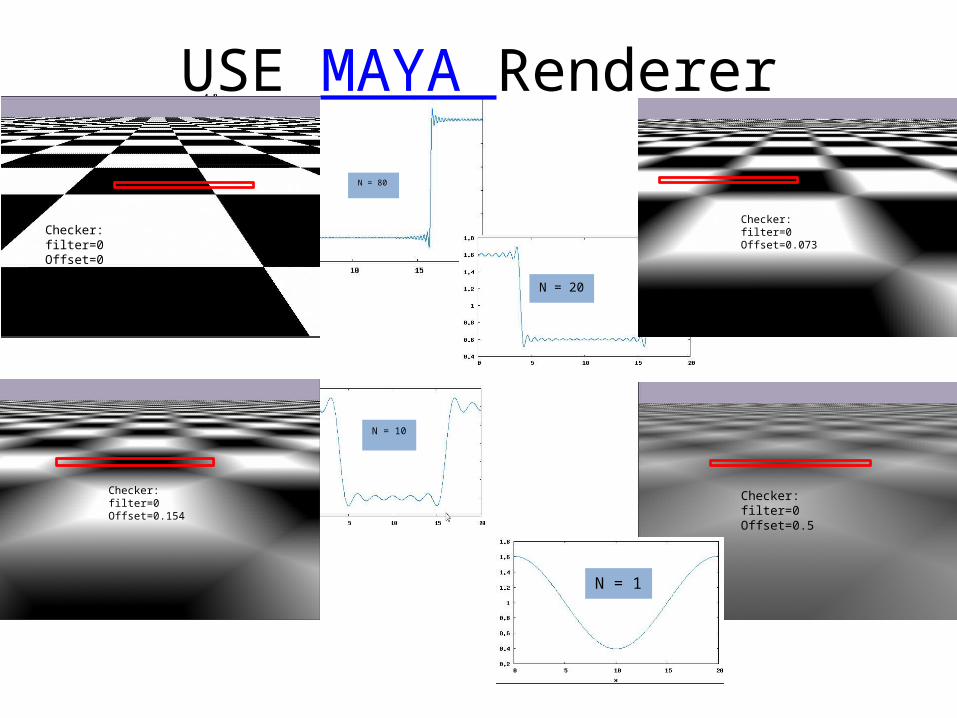
Plotting …N = 1
N = 10
N = 20
N = 80
T=420 (W = 2*/20)
N = 10
N = 80
N = 20
USE MAYA Renderer
Checker: filter=0Offset=0
Checker: filter=0Offset=0.073
Checker: filter=0Offset=0.154
Checker: filter=0Offset=0.5
N = 1
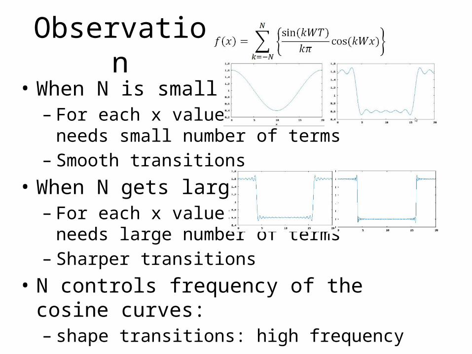
Observation• When N is small– For each x value:
needs small number of terms– Smooth transitions
• When N gets large: – For each x value:
needs large number of terms– Sharper transitions
• N controls frequency of the cosine curves: – shape transitions: high frequency

What have we done?• Took an extremely simple part of an image:– Show how to represent with math
• Analyzed the math expression– Define: high vs. low frequency
• What we did not do:– Show: any given image (function) can be expressed
as a summation of sinusoidal functions– Term: transform an image (function) to frequency
domain (e.g., Fourier Transform)

• We have seen Square signal (function) in 1D:
• Restricting N to small numbers– corresponds to smooth the square corners– Low pass “filtering” (only keep low frequency)
• Restricting N to large numbers– Corresponds to keep only the corners– High pass filtering (only allow high frequency)– E.g., only sum terms – between 100 and 200:
Frequency of A Signal

Frequency “Domain”• Plot the size of the cosine terms of functions!• E.g., the square pulse– Can be expressed as:
Frequency domain is a plot of these terms against k …
Cosine functions: define how fast the signal will vary
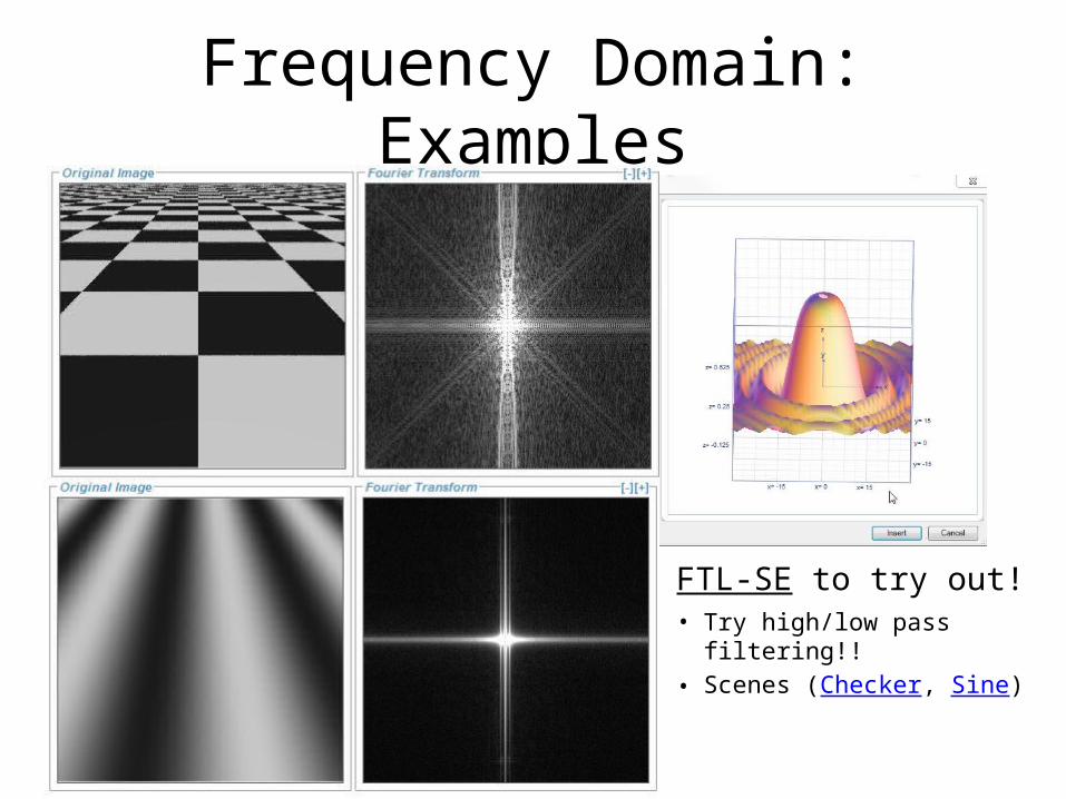
Frequency Domain: Examples
FTL-SE to try out!• Try high/low pass
filtering!!• Scenes (Checker, Sine)

Frequency of an image• High Frequency:– Sharp color changes
• Low Frequency: – Smooth or no change

Sampling Theorem
• Nyquist Frequency: to faithfully capture the signal– Sample at twice the highest frequency in the signal
Intensity of the line
One line of color
Sample at pixel locations
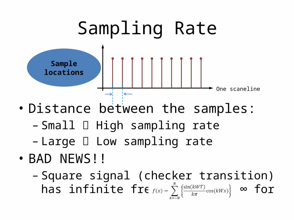
Sampling Rate
• Distance between the samples: – Small High sampling rate– Large Low sampling rate
• BAD NEWS!!– Square signal (checker transition) has infinite
frequency! (N ∞ for
Sample locations
One scaneline