Statistics and Computing manuscript No.(will be inserted by the editor)

Bayesian computation: a summary of the current state, andsamples backwards and forwards

Peter J. Green · Krzysztof Latuszynski · Marcelo Pereyra ·Christian P. Robert

Received: date / Accepted: date

Abstract Recent decades have seen enormous improve-

ments in computational inference for statistical models;

there have been competitive continual enhancements in

a wide range of computational tools. In Bayesian infer-

ence, first and foremost, MCMC techniques have con-

tinued to evolve, moving from random walk proposals

to Langevin drift, to Hamiltonian Monte Carlo, and so

on, with both theoretical and algorithmic innovations

opening new opportunities to practitioners. However,

this impressive evolution in capacity is confronted by an

even steeper increase in the complexity of the datasets

to be addressed. The difficulties of modelling and then

handling ever more complex datasets most likely call

for a new type of tool for computational inference that

dramatically reduces the dimension and size of the raw

data while capturing its essential aspects. Approximatemodels and algorithms may thus be at the core of the

next computational revolution.

Keywords Bayesian analysis · MCMC algorithms ·ABC techniques · optimisation

Supported in part by “SuSTaIn”, EPSRC grantEP/D063485/1, at the University of Bristol, and “i-like”,EPSRC grant EP/K014463/1, at the University of Warwick.Krzysztof Latuszynski holds a Royal Society UniversityResearch Fellowship, and Marcelo Pereyra a Marie CurieIntra-European Fellowship for Career Development. PeterGreen also holds a Distinguished Professorship at UTS,Sydney, and Christian Robert an Institut Universitaire deFrance chair at CEREMADE, Universite Paris-Dauphine.

Peter Green and Marcelo PereyraSchool of Mathematics, University of BristolE-mail: P.J.Green, Marcelo.Pereyra@bristol.ac.uk

Krzysztof Latuszynski and Christian P. RobertDept. of Statistics, University of WarwickE-mail: K.G.Latuszynski@warwick.ac.uk, robert@ensae.fr

1 Introduction

One may reasonably balk at the terms “computational

statistics” and “Bayesian computation” since, from its

very start, statistics has always involved some computa-

tional step to extract information, something manage-

able like an estimator or a prediction, from raw data.

This necessarily incomplete and unavoidably biased re-

view of the recent past, current state, and immediate

future of algorithms for Bayesian inference thus first re-

quires us to explain what we mean by computation in a

statistical context, before turning to what we perceive

as medium term solutions and possible deadends.

Computations are an issue in statistics whenever

processing a dataset becomes a difficulty, a liability,

or even an impossibility. Obviously, the computationalchallenge varies according to the time when it is faced:

what was an issue in the 19th century is most likely not

so any longer (take for instance the derivation of the

moment estimates of a mixture of two normal distribu-

tions so painstakenly set by Pearson (1894) for estimat-

ing the ratio of “forehead” breadth to body length on

a dataset of 1,000 crabs or the intense algebraic deriva-

tions found in the analysis of variance of the 1950s and

1960s (Searle et al. 1992)).

The introduction of simulation tools in the 1940s

followed hard on the heels of the invention of the com-

puter and certainly contributed an impetus towards

faster and better computers, at least in the first decade

of this revolution. This shows that these tools were

both needed, and unavailable without electronic calcu-

lators. The introduction of Markov chain Monte Carlo

is harder to pin down as some partial versions can be

traced all the way back to 1944–45 and the Manhat-

tan project at Los Alamos (Metropolis 1987). It is sur-

prisingly much later, i.e., only by the early 1990s, that

arX

iv:1

502.

0114

8v3

[st

at.C

O]

9 M

ay 2

015

2 P. J. Green, K. Latuszynski, M. Pereyra, & C. P. Robert

such methods became part of the Bayesian toolbox,

that is, some time after the devising of other computer-

dependent tools like the bootstrap or the EM algo-

rithm, and despite the availability of personal comput-

ers that considerably eased programming and exper-

imenting (Robert and Casella 2011). It is presumably

pointless to try to attribute this delay to a definite cause

but a certain lack of probabilistic culture within the

statistics community is probably partly to blame.

What makes this time-lag in MCMC methods be-

coming assimilated into the statistics community even

more surprising is that fact that Bayesian inference

having a significant role in statistical practice was re-

ally on hold pending the discovery of flexible computa-

tional tools that (implictly or explicitly) delivered val-

ues for the medium- to high-dimensional integrals that

underpin the calculation of posterior distributions, in

all but toy problems where conjugacy provided explicit

answers. In fact, until Bayesians discovered MCMC,

the only computational methodology that seemed to

offer much chance of making practical Bayesian statis-

tics practical was the portfolio of quadrature methods

developed under Adrian Smith’s leadership at Notting-

ham (Naylor and Smith 1982; Smith et al. 1985, 1987).

The very first article in the first issue of Statis-

tics and Computing, whose quarter-century we cele-

brate in this special issue, was (to the journal’s credit!)

on Bayesian analysis, and was precisely in this direc-

tion of using clever quadrature methods to approach

moderately high-dimensional posterior analysis (Della-

portas and Wright 1991). By the next (second) issue,

sampling-based methods had started to appear, with

three papers out of five in the issue on or related to

Gibbs sampling (Verdinelli and Wasserman 1991; Car-

lin and Gelfand 1991; Wakefield et al. 1991).

Now, reflecting upon the evolution of MCMC meth-

ods over the 25 or so years they have been at the fore-

front of Bayesian inference, the focus has evolved a long

way, from hierarchical models that extended the lin-

ear, mixed and generalised linear models (Albert 1988;

Carlin et al. 1992; Bennett et al. 1996) which were ini-

tially the focus, and graphical models that stemmed

from image analysis (Geman and Geman 1984) and

artificial intelligence, to dynamical models driven by

ODE’s (Wilkinson 2011b) and diffusions (Roberts and

Stramer 2001; Dellaportas et al. 2004; Beskos et al.

2006), hidden trees (Larget and Simon 1999; Huelsen-

beck and Ronquist 2001; Chipman et al. 2008; Aldous

et al. 2008) and graphs, aside with decision making

in highly complex graphical models. While research on

MCMC theory and methodology is still active and con-

tinually branching (Papaspiliopoulos et al. 2007; An-

drieu and Roberts 2009; Latuszynski et al. 2011; Douc

and Robert 2011), progressively incorporating the ca-

pacities of parallel processors and GPUs (Lee et al.

2009; Jacob et al. 2011; Strid 2010; Suchard et al. 2010;

Scott et al. 2013; Calderhead 2014), we wonder if we

are not currently facing a new era where those meth-

ods are no longer appropriate to undertake the anal-

ysis of new models, and of new formulations where

models are no longer completely defined. We indeed

believe that imprecise models, incomplete information

and summarised data will become, if not already, a cen-

tral aspect of statistical analysis, due to the massive

influx of data and the need to provide non-statisticians

with efficient tools. This is why we also cover in this

survey the notions of approximate Bayesian computa-

tion (ABC) and comment on the use of optimisation

tools.

The plan of the paper is that in Sections 2 and 3 we

discuss recent progress and current issues in Markov

chain Monte Carlo and Approximate Bayesian Com-

putation respectively. In Section 4, we highlight some

araes of modern optimisation that, through lack of fa-

miliarity, are making less impact in the mainstream of

Bayesian computation than we think justified. Our Dis-

cussion in Section 5 raises issues about data science and

relevance to applications, and looks to the future.

2 MCMC, targetting the posterior

When MCMC techniques were introduced to the main-

stream statistical (Bayesian) community in 1990, they

were received with skepticism that they could one day

become the central tool of Bayesian inference. For in-

stance, despite the assurance provided by the ergodic

theorem, many researchers thought at first that the

convergence of those algorithms was a mere theoreti-

cal anticipation rather than a practical reality, in con-

trast to traditional Monte Carlo methods, and hence

that they could not be trusted to provide “exact” an-

swers. This perspective is obviously obsolete by now,

when MCMC output is considered as “exact” as regular

Monte Carlo, if possibly less efficient in some settings.

Nowadays, MCMC is again attracting more attention

(than in the past decade, say, where developments were

more about alternatives, some of which described in

the following sections), both because of methodologi-

cal developments linked to better theoretical tools, for

instance in the handling of stochastic processes, and

because of new advances in accelerated computing via

parallel and cloud computing.

Bayesian computation: a summary of the current state, and samples backwards and forwards 3

2.1 Basics of MCMC

The introduction of Markov chain based methods within

Monte Carlo thus took a certain amount of argument

to reach the mainstream statistical community, when

compared with other groups who were using MCMC

methods 10 to 30 years earlier. It may sound unlikely

at the current stage of our knowledge, but using meth-

ods that (a) generated correlated output, (b) required

some burnin time to remove the impact of the initial

distribution and (c) did not lead to a closed form ex-

pression for asymptotic variances were indeed met with

resistance at first. As often, the immense computing

advantages offered by this versatile tool soon overcame

the reluctance to accept those methods as similarly “ex-

act” as other Monte Carlo techniques, applications driv-

ing the move from the early 1990s. We reproduce be-

low the generic version of the “all variables at once”

Metropolis–Hastings algorithm (Metropolis et al. 1953;

Hastings 1970; Besag et al. 1995; Robert and Casella

2011) as it (still) constitutes in our opinion a fundamen-

tal advance in computational statistics, namely that,

given a computable density π (up to a normalising con-

stant) on Θ, and a proposal Markov kernel q(·|·), there

exists a universal machine that returns a Markov chain

with the proper stationary distribution, hence an asso-

ciated operational MCMC algorithm.

Algorithm 1 Metropolis–Hastings algorithm (generic

version)

Choose a starting value θ(0))for n = 1 to N do

Generate θ∗ from a proposal q(·|θ(n−1))Compute the acceptance probability

ρ(n) = 1 ∧ π(θ∗) q(θ(n−1)|θ∗))/π(θ(n−1)q(θ∗|θ(n−1))

Generate un ∼ U(0, 1) and take θ(n) = θ∗ if un ≤ ρ(n),θ(n) = θ(n−1) otherwise.

end for

The first observation about the Metropolis–Hastings

is that the flexibility in choosing q is a blessing, but also

a curse since the choice determines the performance of

the algorithm. Hence a large part of the research on

MCMC along the past 30 years (if we arbitrarily set

the starting date at Geman and Geman (1984)) has

been on choice of the proposal q to improve the effi-

ciency of the algorithm, and in characterising its con-

vergence properties. This typically requires gathering

or computing additional information about π and we

discuss some of the fundamental strategies in subse-

quent sections. Algorithm 1, and its variants in which

variables are updated singly or in blocks according to

some schedule, remains a keystone in standard use of

MCMC methodology, even though the newer Hamil-

tonian Monte Carlo approach (see Section 2.3) may

sooner or later come to replace it. While there is noth-

ing intrinsically unique to the nature of this algorithm,

or optimal in its convergence properties (other than the

result of Peskun (1973) on the optimality of the accep-

tance ratio), attempts to bypass Metropolis–Hastings

are few and limited. For instance, the birth-and-death

process developed by Stephens (2000) used a continu-

ous time jump process to explore a set of models, only

to be later shown (Cappe et al. 2002) to be equivalent

to the (Metropolis–Hastings) reversible jump approach

of Green (1995).

Another aspect of the generic Metropolis–Hastings

that became central more recently is that while the

accept–reject step does overcome need to know the nor-

malising constant, it still requires π, if unnormalised,

and this may be too expensive to compute or even in-

tractable for complicated models and large datasets.

Much recent research effort has been devoted to the

design and understanding of appropriate modifications

that use estimators or approximations of π instead and

we will take the opportunity to summarise some of the

progress in this direction.

2.2 MALA and Manifold MALA

Stochastic differential equations (SDEs) have been and

still are informing Monte Carlo development in a num-

ber of seminal ways. A key insight is that the Langevin

diffusion on Θ solving

dθt =1

2∇ log π(θt)dt+ dBt (1)

has π as its stationary and limiting distribution. Here

Bt is the standard Brownian motion and ∇ denotes

gradient. The crude approach of sampling an Euler dis-

cretisation (Kloeden and Platen (1992)) of (1) and us-

ing it as an approximate sample from π was introduced

in the applied literature (Ermak (1975); Doll and Dion

(1976)). The method results in a Markov chain evolving

according to the dynamics

θ(n)|θ(n−1) ∼ Q(θ(n−1), ·)

:= θ(n−1) +h

2∇ log π(θ(n−1)) (2)

+ h1/2N(0, Id×d),

for a chosen discretisation step h. There is a delicate

tradeoff between accuracy of the approximation im-

proving as h → 0 and sampling efficiency (as mea-

sured e.g. by the effective sample size) improving when

4 P. J. Green, K. Latuszynski, M. Pereyra, & C. P. Robert

h increases. This solution was soon followed by its Me-

tropolised version (Rossky et al. (1978)) that uses the

Euler approximation of (2) to produce a proposal in the

Metropolis–Hastings algorithm 1, by letting q(·|θ(n−1)) :=

θ(n−1)+ h2∇ log π(θ(n−1))+h1/2N(0, Id×d). While in the

probability community Langevin diffusions and their

equilibrium distributions had also been around for some

time (Kent (1978)), it was the Roberts and Tweedie

(1996a) paper (motivated by Besag (1994) comment

on Grenander and Miller (1994)) that brought the ap-

proach to the centre of interest of the computational

statistics community and sparked systematic study, de-

velopment and applications of Metropolis adjusted Langevin

algorithms (hence MALA) and their cousins.

There is a large body of empirical evidence that

at the extra price of computing the gradient, MALA

algorithms typically provide a substantial speed-up in

convergence on certain types of problems. However for

very light-tailed distributions the drift term may grow

to infinity and cause additional instability. More pre-

cisely, for distributions with sufficiently smooth con-

tours, MALA is geometrically ergodic (c.f. Roberts and

Rosenthal (2004)) if the tails of π decay as exp{−|θ|β}with β ∈ [1, 2], while the random walk Metropolis al-

gorithm is geometrically ergodic for all β ≥ 1 (Roberts

and Tweedie (1996a); Mengersen and Tweedie (1996)).

The lack of geometrical ergodicity has been precisely

quantified by Bou-Rabee and Hairer (2012).

Various refinements and extensions have been pro-

posed. These include optimal scaling and choice of the

discretisation step h, adaptive versions (both discussed

in Section 2.4), combinations with proximal operators

(Pereyra 2015; Schreck et al. 2013), and applications

and algorithm development for the infinite-dimensional

context (Pillai et al. 2012; Cotter et al. 2013). One par-

ticular direction of active research is considering a more

general version of equation (1) with state-dependent

drift and diffusion coefficient

dθt =(σ(θt)

2∇ log π(θt) +

γ(θt)

2

)dt+

√σ(θt)dBt (3)

γi(θt) =∑j

∂σij(θt)

∂θj,

which also has π as invariant distribution (Xifara et al.

(2014), c.f. Kent (1978)). The resulting proposals are

q(·|θ(n−1)) :=h

2

(σ(θ(n−1))∇ log π(θ(n−1)) + γ(θ(n−1))

)+h1/2N(0, σ(θ(n−1))) + θ(n−1).

Choosing appropriate σ for improved ergodicity is how-

ever nontrivial. The idea has been explored in Stramer

and Tweedie (1999a,b); Roberts and Stramer (2002)

and more recently Girolami and Calderhead (2011) in-

troduced a mathematically-coherent approach of relat-

ing σ to a metric tensor on a Riemannian manifold of

probability distributions. The resulting algorithms are

termed Manifold MALA (MMALA), Simplified MMALA

(Girolami and Calderhead 2011), and position-dependent

MALA (PMALA) (Xifara et al. 2014), and differ in im-

plementation cost, depending on how precise is the use

they make of versions of equation (3). The approach

still leaves the specification of the metric to be used in

the space of probability distributions to the user, how-

ever there are some natural choices. One can, for exam-

ple, take the Hessian of π and replace its eigenvalues

by their absolute values λi → |λi|. Building the metric

tensor from this spectrally-positive version of the Hes-

sian of π and randomising the discretisation step size h

results in an algorithm that is as robust as random walk

Metropolis, in the sense that it is geometrically ergodic

for targets with tail decay of exp{−|θ|β} for β > 1 (see

Taylor (2014)). A robustified version of such a metric

has been introduced in Betancourt (2013) and termed

SoftAbs. Here one approximates the absolute value of

the eigenspectrum of the Hessian of π with a smooth

strictly positive function λi → λiexp {αλi}+exp {−αλi}exp {αλi}−exp {−αλi} ,

where α is a smoothing parameter. The metric sta-

bilises the behaviour of both MMALA, and Hamilto-

nian Monte Carlo algorithms (discussed in the sequel),

in the neighbourhoods where the signature of the Hes-

sian changes.

2.3 Hamiltonian Monte Carlo

As with many improvements in the literature, starting

with the very notion of MCMC, Hamiltonian (or hy-

brid) Monte Carlo (HMC) stems from Physics (Duane

et al. 1987). After a slow emergence into the statistical

community (Neal 1999), it is now central in statistical

software like STAN (Stan Development Team 2014).

For a complete account of this important flavour of

MCMC, the reader is referred to Neal (2013), which in-

spired the description below; see also Betancourt et al.

2014 for a highly mathematical differential-geometric

approach to HMC.

This method can be seen as a particular and effi-

cient instance of auxiliary variables (see, e.g., Besag and

Green 1993 and Rubinstein 1981), in which we apply a

deterministic-proposal Metropolis method to the aug-

mented target. In physical terms, the idea behind HMC

is to add a “kinetic energy” term to the “potential en-

ergy” (negative log-target), leading to the Hamiltonian

H(θ, p) = − log π(θ) + pTM−1p/2

Bayesian computation: a summary of the current state, and samples backwards and forwards 5

where θ denotes the object to be simulated (i.e., the pa-

rameter), p its speed or momentum and M the Hamil-

tonian matrix of π. In more statistical language, HMC

creates an auxiliary variable p such that moving accord-

ing to Hamilton’s equations

θ

dt=∂H

∂p=∂H

∂p= M−1p

dp

dt= −∂H

∂θ=∂ log π

∂θ

preserves the joint distribution with density exp{−H(θ,

p)}, hence the marginal distribution of θ, that is, π(θ).

Hence, if we could simulate exactly this joint distri-

bution of (θ, p), a sample from π(θ) would be a by-

product. However, in practice, the equation is solved

approximately and hence requires a Metropolis correc-

tion. As discussed in, e.g., Neal (2013), the dynam-

ics induced by Hamilton’s equations is reversible and

volume-preserving in the (θ, p) space, which means in

practice that there is no need for a Jacobian in Metropo-

lis updates. The practical implementation relies on a

k−th order symplectic integrator (Hairer et al. 2006),

most commonly on the 2-nd order leapfrog approxima-

tion that relies on a small step level ε, updating p and θ

via a modified Euler’s method called the leapfrog that

is reversible and being symplectic, preserves volume as

well. This discretised update can be repeated for an

arbitrary number of steps.

When considering the implementation via a Metropo-

lis algorithm, a new value of the momentum p is drawn

from the pseudo-prior ∝ exp{−pTM−1p/2} and it is

followed by a Metropolis step, which proposal is driven

by the leapfrog approximation to the Hamiltonian dy-

namics on (θ, p) and which acceptance is governed by

the Metropolis acceptance probability. What makes the

potential strength of this augmentation (or dis-integra-

tion) scheme is that the value of H(θ, p) hardly changes

during the Metropolis move, which means that it is

most likely to be accepted and that it may produce a

very different value of π(θ) without modifying the over-

all acceptance probability. In other words, moving along

level sets is almost energy-free, but if the move proceeds

for “long enough”, the chain can reach far-away regions

of the parameter space, thus avoid the myopia of stan-

dard MCMC algorithms. As explained in Neal (2013),

this means that Hamiltonian Monte Carlo avoids the

inefficient random walk behaviour of most Metropolis–

Hastings algorithms. What drives the exploration of the

different values of H(θ, p) is therefore the simulation of

the momentum, which makes its calibration both quite

influential and delicate (Betancourt et al. (2014)) as it

depends on the unknown normalising constant of the

target. (By calibration, we mean primarily the choice

of the time discretisation step ε in the leapfrog approx-

imation and of the number L of leapfrog leaps, but also

the choice of the precision matrix M .)

2.4 Optimal scaling and Adaptive MCMC

The convergence of the Metropolis-Hastings algorithm 1

depends crucially on the choice of the proposal distribu-

tion q, as does the performance of both more complex

MCMC and SMC algorithms, that often are hybrids

using Metropolis–Hastings as simulation substeps.

Optimising over all implementable q appears to be a

“disaster problem” due to its infinite-dimensional char-

acter, lack of clarity about what is implementable, what

is not, and the fact that this optimal q must depend in

a complex way on the target π to which we have only

a limited access. In particular MALA provides a spe-

cific approach to constructing π-tailored proposals and

HMC can be viewed as a combination of Gibbs and

special Metropolis moves for an extended target.

In this optimisation context, it is thus reasonable to

restrict ourselves to some parametric family of propos-

als qξ, or more generally of Markov transition kernels

Pξ, where ξ ∈ Ξ is a tuning parameter, possibly high-

dimensional.

The aim of adaptive Markov chain Monte Carlo is

conceptually very simple. One expects that there is a

set Ξπ ⊂ Ξ of good parameters ξ for which the kernel

Pξ converges quickly to π, and one allows the algorithm

to search for Ξπ “on the fly” and redesign the transition

kernel during the simulation as more and more infor-

mation about π becomes available. Thus an adaptive

MCMC algorithm would apply the kernel Pξ(n) to sam-

ple θ(n) given θ(n−1), where the tuning parameter ξ(n)

is itself a random variable which may depend on the

whole history θ(0), . . . , θ(n−1) and on ξ(n−1). Adaptive

MCMC rests on the hope that the adaptive parame-

ter ξ(n) will find Ξπ, stay there essentially forever and

inherit good convergence properties.

There are at least two fundamental difficulties in ex-

ecuting this strategy in practice. First, standard mea-

sures of efficiency of Markovian kernels, like the to-

tal variation convergence rate (c.f. Meyn and Tweedie

(2009); Roberts and Rosenthal (2004)), L2(π) spectral

gap (Diaconis and Stroock (1991); Roberts (1996); Saloff-

Coste (1997); Levin et al. (2009)) or asymptotic vari-

ance (Peskun (1973); Geyer (1992); Tierney (1998)) in

the Markov chain central limit theorem will not be

available explicitly, and their estimation from a Markov

chain trajectory is often an even more challenging task

than the underlying MCMC estimation problem itself.

Secondly, when executing an adaptive strategy and

trying to improve the transition kernel on the fly, the

6 P. J. Green, K. Latuszynski, M. Pereyra, & C. P. Robert

Markov property of the process is violated, therefore

standard theoretical tools do not apply, and establish-

ing validity of the approach becomes significantly more

difficult. While the approach has been successfully ap-

plied in some very challenging practical problems (Solo-

nen et al. (2012); Richardson et al. (2010); Griffin et al.

(2014)), there are examples of seemingly reasonable adap-

tive algorithms that fail to converge to the intended

target distribution (Bai et al. (2011); Latuszynski et al.

(2013)), indicating that compared to standard MCMC

even more care must be taken to ensure validity of in-

ferential conclusions.

While heuristics-based adaptive algorithms have been

considered already in Gilks et al. (1994), a remarkable

result providing a tool to address the difficulty of op-

timising Markovian kernels coherently is the Roberts

et al. (1997) paper on scaling the proposal variance. It

considers settings of increasing dimensionality and in-

vestigates efficiency of the random walk Metropolis al-

gorithm as a function of its average acceptance rate.

More specifically, given a sequence of targets πd on

the product state space Θd with iid components con-

structed from conveniently smooth marginal f,

πd(θ) :=

d∏i=1

f(θi), for d = 1, 2, . . . (4)

consider a sequence of Markov chains θd, d = 1, 2, . . . ,

where the chain θd = (θ(n)d )n=0,1,... is a random walk

Metropolis targeting πd with proposal increments dis-

tributed as N(0, σ2dId×d).

It then turns out that the only sensible scaling of

the proposal as dimensionality increases is to take σ2d =

l2d−1. In this regime the sequence of time-rescaled first

coordinate processes

Z(t)d := θ

(btdc)d,1 , for d = 1, 2, . . .

converges in a suitable sense to the solution Z of a

stochastic differential equation

dZt = h(l)1/2dBt +1

2h(l)∇ log f(Zt)dt.

Hence maximising the speed of the above diffusion h(l)

is equivalent to maximising the efficiency of the algo-

rithm as the dimension goes to infinity. Surprisingly,

there is a one-to-one correspondence between the value

lopt = argmaxh(l) and the mean acceptance probability

of 0.234.

The magic number 0.234 does not depend on f and

gives a universal tuning recipe to be used for example

in adaptive algorithms: choose the scale of the incre-

ment so that approximately 23% of the proposals are

accepted.

The result, established under restrictive assumptions,

has been empirically verified to hold much more gener-

ally, for non iid targets and also in medium- and even

low-dimensional examples with d as small as 5. It has

been also combined with relative efficiency loss due to

mismatch between the proposal and target covariance

matrices (see Roberts and Rosenthal (2001)).

The simplicity of the result and easy access to the

average acceptance rate makes optimal scaling the main

theoretical driver in development of adaptive MCMC

algorithms, and adaptive MCMC is the main applica-

tion and motivation for researching optimal scaling.

A large body of theoretical work extends optimal

scaling formally to different and more general scenarios.

For example Metropolis for smooth non iid targets has

been addressed e.g. by Bedard (2007), and in infinite

dimensional settings by Beskos et al. (2009). Discrete

and other discontinuous targets have been considered in

Roberts (1998) and Neal et al. (2012). For MALA al-

gorithms an optimal acceptance rate of 0.574 has been

established in Roberts and Rosenthal (1998) and con-

firmed in infinite-dimensional settings in Pillai et al.

(2012) along with the stepsize σ2d = l2d−1/3. Hybrid

Monte Carlo (see Section 2.3) has been analysed in a

similar spirit by Beskos et al. (2013) and Betancourt

et al. (2014) concluding that any value ∈ [0.6, 0.9] will

be close to optimal and the leapfrog step size should be

taken as h = l × d−1/4. These results not only inform

about optimal tuning, but also provide an efficiency or-

dering on the algorithms in d−dimensions. Metropolis

algorithms need O(d) steps to explore the state space,

while MALA and HMC need respectively O(d1/3) and

O(d1/4).

Further extensions include studying the transient

phase before reaching stationarity (Christensen et al.

(2005); Jourdain et al. (2012, 2014)), the scaling of

multiple-try MCMC (Bedard et al. (2012)) and delayed

rejection MCMC (Bedard et al. (2014)), and the tem-

perature scale of parallel tempering type algorithms

(Atchade et al. (2011b); Roberts and Rosenthal (2014)).

Interestingly, the optimal scaling of the discussed in

Section 2.5 pseudo-marginal algorithms as obtained in

Sherlock et al. (2014), and extended to more general

settings in Doucet et al. (2012); Sherlock (2014), sug-

gests an acceptance rate of just 0.07.

While each of these numerous optimal scaling re-

sults gives rise, at least in principle, to an adaptive

MCMC design, the pioneering and most successful algo-

rithm is the Adaptive Metropolis of Haario et al. (2001).

With its increasing popularity in applications, this has

fuelled the development of the field.

Here one considers a normal increment proposal that

estimates the target covariance matrix from past sam-

ples and applies appropriate dimension-dependent scal-

ing and covariance shrinkage. Precisely, the proposal

Bayesian computation: a summary of the current state, and samples backwards and forwards 7

takes the form

q(·|θ(n−1)) = N(θ(n−1), C(n)), (5)

with the covariance matrix

C(n) =(2.38)2

d

(ˆcov(θ(0), . . . , θ(n−1)) + εId×d

)(6)

which is efficiently computed using a recursive formula.

Versions and refinements of the adaptive Metropolis

algorithm (Roberts and Rosenthal 2009; Andrieu and

Thoms 2008) have served well in applications and mo-

tivated much of the theoretical development. These in-

clude, among many other contributions, adaptive Metropo-

lis, delayed rejection adaptive Metropolis (Haario et al.

(2006)), regional adaptation and parallel chains (Craiu

et al. 2009), and the robust version of Vihola (2012)

estimating the shape of the distribution rather than its

covariance matrix and hence suitable for heavy tailed

targets.

Analogous development of adaptive MALA algo-

rithms in Atchade (2006); Marshall and Roberts (2012)

and of adaptive Hamiltonian and Riemannian Manifold

Monte Carlo in Wang et al. (2013) building on the adap-

tive scaling theory, resulted in a similar drastic mixing

improvement as the original Adaptive Metropolis.

Another substantial and still unexplored area where

adaptive algorithms are applied for very high dimen-

sional and multimodal problems is model and variable

selection (Nott and Kohn (2005); Richardson et al. (2010);

Lamnisos et al. (2013); Ji and Schmidler (2013); Grif-

fin et al. (2014)). These algorithms can incorporate re-

versible jump moves (Green 1995) and are guided by

scaling limits for discrete distributions as well as tem-

perature spacing of parallel tempering to address mul-

timodality. Successful implementations allow for fully

Bayesian variable selection in models with over 20 000

variables for which otherwise only ad hoc heuristic ap-

proaches have been used in the literature.

To address the second difficulty with adaptive algo-

rithms, several approaches have been developed to es-

tablish their theoretical underpinning. While for stan-

dard MCMC, convergence in total variation and law

of large numbers are obtained almost trivially, and the

effort concentrates on stronger results, like CLTs, geo-

metric convergence, nonasymptotic analysis, and, maybe

most importantly, comparison and ordering of algorithms,

adaptive samplers are intrinsically difficult. The most

elegant and theoretically-valid strategy is to change the

underlying Markovian kernel at regeneration times only

(Gilks et al. (1998)). Unfortunately, this is not very ap-

pealing for practitioners since regenerations are diffi-

cult to identify in more complex settings and are essen-

tially impractically rare in high dimensions. The orig-

inal Adaptive Metropolis of Haario et al. (2001) has

been validated (under some restrictive additional con-

ditions) by controlling the dependencies introduced by

the adaptation and using convergence results for mixin-

gales. The approach has been further developed in Atchade

and Rosenthal (2005) and Atchade (2006) to verify its

ergodicity under weaker assumptions and apply the mixin-

gale approach to adaptive MALA. Another successful

approach (Andrieu and Moulines (2006) refined in Saks-

man and Vihola (2010)) rests on martingale difference

approximations and martingale limit theorems to ob-

tain, under suitable technical assumptions, versions of

LLN and CLTs. There are close links between analysing

adaptive MCMC and stochastic approximation algo-

rithms and in particular the adaptation step can be

often written as a mean field of the stochastic approxi-

mation procedure; Andrieu and Robert (2001); Atchade

et al. (2011a); Andrieu et al. (2015) contribute to this

direction of analysis. Fort et al. (2011) develop an ap-

proach where both adaptive and interacting MCMC al-

gorithms can be treated in the same framework. This al-

lows addressing “external adaptation” algorithms such

as the interacting tempering algorithm (a simplified

version of the celebrated equi-energy sampler of Kou

et al. (2006)) or adaptive parallel tempering in Miaso-

jedow et al. (2013).

We present here the rather general but fairly simple

coupling approach (Roberts and Rosenthal (2007)) to

establishing convergence. Successfully applied to a va-

riety of adaptive Metropolis samplers under weak regu-

larity conditions (Bai et al. (2011)), adaptive Gibbs and

adaptive Metropolis within adaptive Gibbs samplers

( Latuszynski et al. (2013)), it shows that two prop-

erties Diminishing Adaptation and Containment are

sufficient to guarantee that an adaptive MCMC algo-

rithm will converge asymptotically to the correct target

distribution. To this end recall the total variation dis-

tance between two measures defined as ‖ν(·)−µ(·)‖ :=

supA∈F |ν(A)−µ(A)|, and for every Markov transition

kernel Pξ, ξ ∈ Ξ and every starting point θ ∈ Θ define

the ε convergence function Mε : Θ ×Ξ → N as

Mε(θ, ξ) := inf{n ≥ 1 : ‖P (n)ξ (θ, ·)− π(·)‖ ≤ ε}.

Let {(θ(n), ξ(n))}∞n=0 be the corresponding adaptive MCMC

algorithm and by A(n)((θ, ξ), ·) denote its marginal dis-

tribution at time t, i.e.

A(n)((θ, ξ), B) := P(θ(n) ∈ B|θ(0) = θ, ξ(0) = ξ).

The adaptive algorithm is ergodic for every starting val-

ues of θ and ξ if limn→∞ ‖A(n)((θ, ξ, ·)−π(·)‖ = 0. The

two conditions guaranteeing ergodicity are

Definition 1 (Diminishing Adaptation) The adap-

tive algorithm with starting values θ(0) = θ and ξ(0) = ξ

8 P. J. Green, K. Latuszynski, M. Pereyra, & C. P. Robert

satisfies Diminishing Adaptation, if

limn→∞

D(n) = 0 in probability, where

D(n) := supθ∈Θ‖Pξ(n+1)(θ, ·)− Pξ(n)(θ, ·)‖.

Definition 2 (Containment) The adaptive algorithm

with starting values θ(0) = θ and ξ(0) = ξ satisfies Con-

tainment, if for all ε > 0 the sequence {Mε(θ(n), ξ(n))}∞n=0

is bounded in probability.

While diminishing adaptation is a standard require-

ment, Containment is subject to some discussion. On

one hand, it may seem difficult to verify in practice; on

the other, it may appear restrictive in the context of er-

godicity results under some weaker conditions (c.f. Fort

et al. (2011)). However, it turns out ( Latuszynski and

Rosenthal (2014)) that if Containment is not satisfied,

then the algorithm may still converge, but with posi-

tive probability it will be asymptotically less efficient

than any nonadaptive ergodic MCMC scheme. Hence

algorithms that do not satisfy Containment are termed

AdapFail and are best avoided. Containment has been

further studied in Bai et al. (2011) and is in particular

implied by simultaneous geometric or polynomial drift

conditions of the adaptive kernels.

Given that adaptive algorithms may be incorpo-

rated in essentially any sampling scheme, their intro-

duction seems to be one of the most important inno-

vations of the last two decades. However, despite sub-

stantial effort and many ingenious contributions, the

theory of adaptive MCMC lags behind practice even

more than may be the case in other computational ar-

eas. While theory always matters, the numerous unex-

pected and counterintuitive examples of transient adap-

tive algorithms suggest that in this area theory matters

even more for healthy development.

For adaptive MCMC to become a routine tool, a

clear-cut result is needed saying that under some eas-

ily verifiable conditions these algorithms are valid and

perform not much worse than their nonadaptive coun-

terpart with fixed parameters. Such a result is yet to be

established and may require deeper understanding of

how to construct stable adaptive MCMC, rather than

aiming heavy technical artillery at algorithms currently

in use without modifying them.

2.5 Estimated likelihoods and pseudo-marginals

There are numerous settings of interest where the tar-

get density π(·|y) is not available in closed form. For

instance, in latent variable models, the likelihood func-

tion `(θ|y) is often only available as an intractable in-

tegral

`(θ|y) =

∫Zg(z, y|θ) dz ,

which leads to

π(θ|y) ∝ π(θ)

∫Zg(z, y|θ) dz

being equally intractable. A solution proposed from the

early days of MCMC (Tanner and Wong 1987) is to con-

sider z as an auxiliary variable and to simulate the joint

distribution π(θ, z|y) on Θ ×Z by a standard method,

leading to simulating the marginal density π(·|y) as a

by-product. However, when the dimension of the aux-

iliary variable z grows with the sample size, this tech-

nique may run into difficulties as induced MCMC al-

gorithms are more and more likely to have convergence

issues. An illustration of this case is provided by hid-

den Markov models, which have eventually to resort to

particle filters as Markov chain algorithms become in-

effective (Chopin 2007; Fearnhead and Clifford 2003).

Another situation where the target density π(·|y) can-

not be directly computed is the case of the “doubly

intractable” likelihood (Murray et al. 2006a), when the

likelihood function `(θ|y) ∝ g(y|θ) itself contains a term

that is intractable, in that it makes the normalising con-

stant

Z(θ) =

∫Yg(y|θ) dy

impossible to compute. The resulting posterior writes

π(θ|y) =π(θ)g(y|θ)Z(θ)p(y)

, where

p(y) =

∫Θ

π(θ)g(y|θ)Z(θ)

dθ,

and consequently the Metropolis-Hastings acceptance

rate becomes

α(θ, θ′) = min

{1,π(θ′)g(y, θ′)q(θ′|θ)π(θ)g(y, θ)q(θ|θ′)

× Z(θ)

Z(θ′)

},

and cannot be evaluated exactly for algorithmic pur-

poses.

Examples of this kind abound in Markov random

fields models, as for instance for the Ising model (Mur-

ray et al. 2006b; Møller et al. 2006).

Both the approaches of Murray et al. (2006a) and

Møller et al. (2006) require sampling data from the like-

lihood `(θ|y), which limits their applicability. The latter

uses in addition an importance sampling function and

may suffer from poor acceptance rates.

Andrieu and Roberts (2009) propose a more general

resolution of such problems by designing a Metropolis–

Hastings algorithm that replaces the intractable tar-

get density π(·|y) with an unbiased estimator, following

Bayesian computation: a summary of the current state, and samples backwards and forwards 9

an idea of Beaumont (2003). The approach is termed

pseudo-marginal. Rather than evaluating the posterior

exactly, a positive unbiased estimate Sθ of π(θ|y) is

utilised. More formally, a new Markov chain is con-

structed that evolves on the extended state space Θ ×R+, where at iteration n, given the pair (θ(n−1), S

(n−1)

θ(n−1))

of parameter value and density estimate at this value,

the proposal (θ′, Sθ′) is obtained by sampling θ′ ∼ q(·|θ(n−1))

and obtaining Sθ′ , the estimate of π(θ′|y). Analogously

to the standard Metropolis-Hastings step, the pair (θ′, Sθ′)

is accepted as (θ(n), S(n)

θ(n)) with probability

min

{1,

Sθ′q(θ(n−1)|θ′)

S(n−1)

θ(n−1)q(θ′|θ(n−1))

},

otherwise the proposal is rejected and the new value set

as (θ(n), S(n)

θ(n)) := (θ(n−1), S(n−1)

θ(n−1)).

It is not difficult to verify that the bivariate chain on

extended state space Θ × R+ enjoys the correct π(θ|y)

marginal on Θ and the approach is valid, see Andrieu

and Roberts (2009)) for details (and also Andrieu and

Vihola (2015) for an abstracted account).

One specific instance of constructing unbiased esti-

mators of the posterior is presented in Girolami et al.

(2013) and based on random truncations of infinite se-

ries expansions. The paper also offers an excellent overview

of inference methods for intractable likelihoods.

The performance of the pseudo-marginal approach

will depend on the quality of the estimators Sθ and

hence stabilising them as well as understanding this re-

lationship is an active area of current development. Of-

ten Sθ is constructed as an importance sampler based

on an importance sample z. Thus in particular, the im-

provements from using multiple samples of z to esti-

mate π are of interest and can be assessed from Andrieu

and Vihola (2015) where the efficiency of the algorithm

is studied in terms of its spectral gap and CLT asymp-

totic variance. Sherlock et al. (2014), Doucet et al. (2012)

and Sherlock (2014), on the other hand, investigate the

efficiency as a function of the acceptance rate and vari-

ance of the noise, deriving the optimal scaling, as dis-

cussed in Section 2.4.

As an alternative to the above procedure of using

estimates of the intractable likelihood to design a new

Markov chain on an extended state space with correct

marginal, one could naively use these estimates to ap-

proximate the Metropolis-Hastings accept-reject ratio

and let the Markov chain evolve in the original state

space. This would amount to dropping the current re-

alisation of Sθ and obtaining a new one in each accept-

reject attempt. Such a procedure is termed Monte Carlo

within Metropolis (Andrieu and Roberts 2009). Unfor-

tunately this approach does not preserve the station-

ary distribution, and the resulting Markov chain may

even not be ergodic (Medina-Aguayo et al. 2015). If

ergodic, the difference between stationary distribution,

resulting from the noisy acceptance must be quantified,

which is a highly nontrivial task and the bounds will

rarely be tight (see also Alquier et al. (2014); Pillai and

Smith (2014); Rudolf and Schweizer (2015) for related

methodology and theory). The approach is however an

interesting avenue since at the price of being biased,

it overcomes mixing difficulties of the exact pseudo-

marginal version.

Design and understanding of pseudo-marginal algo-

rithms is a direction of dynamic methodological devel-

opment that in the coming years will be further fu-

elled not only by complex models with intractable like-

lihoods, but also by the need of MCMC algorithms for

Big Data. In this context the likelihood function cannot

be evaluated for the whole dataset even in the iid case

just because computing the long product of individual

likelihoods is infeasible. Several Big Data MCMC ap-

proaches have been already considered in Welling and

Teh (2011); Korattikara et al. (2013); Teh et al. (2014);

Bardenet et al. (2014); Maclaurin and Adams (2014);

Minsker et al. (2014); Quiroz et al. (2014); Strathmann

et al. (2015).

2.6 Particle MCMC

While we refrain from covering particle filters here, since

others (Beskos et al. 2015) in this volume are focussing

on this technique, a recent advance at the interface be-

tween MCMC, pseudo-marginals, and particle filtering

is the notion of particle MCMC (or pMCMC), devel-

oped by Andrieu et al. (2011). This innovation is in-

deed rather similar to the pseudo-marginal algorithm

approach, taking advantage of the state-space models

and auxiliary variables used by particle filters. It differs

from standard particle filters in that it targets (mostly)

the marginal posterior distribution of the parameters.

The simplest setting in which pMCMC applies is one

of a state-space model where a latent sequence x0:T is

a Markov chain with joint density

p0(x0|θ)p1(x1|x0, θ)) · · · pT (xT |xT−1, θ) ,

and is associated with an observed sequence y1:T such

that

y1:T |x1:T , θ ∼T∏i=1

qi(yi|xi, θ) .

The iterations of pMCMC are MCMC-like in that, at

iteration t, a new value θ′ of θ is proposed from an arbi-

trary transition kernel h(·|θ(t)) and then a new value of

the latent series x′0:T is generated from a particle filter

10 P. J. Green, K. Latuszynski, M. Pereyra, & C. P. Robert

approximation of p(x0:T |θ′, y1:T ). Since the particle fil-

ter returns as a by-product (Del Moral et al. 2006) an

unbiased estimator of the marginal posterior of y1:T ,

q(y1:T |θ′), this estimator can be used as such in the

Metropolis–Hastings ratio

q(y1:T |θ′)π(θ′)h(θ(t)|θ′)q(y1:T |θ)π(θ(t))h(θ′|θ(t))

∧ 1 .

Its validity follows from the general argument of An-

drieu and Roberts (2009), although some additional

(notational) effort is needed to demonstrate all random

variables used therein are correctly assessed (see An-

drieu et al. 2011 and Wilkinson 2011a, the latter pro-

viding a very progressive introduction to the notions of

pMCMC and particle Gibbs, which helped greatly in

composing this section). Note however that the general

validation of pMCMC as targetting the joint posterior

of the states and parameters and of the parallel parti-

cle Gibbs sampler does not follow from pseudo-marginal

arguments.

This approach is being used increasingly in com-

plex dynamic models like those found in signal process-

ing (Whiteley et al. 2010), dynamical systems like the

PDEs in biochemical kinetics (Wilkinson 2011b) and

probabilistic graphical models (Lindsten et al. 2014).

An extension to approximating the sequential filtering

distribution is found in Chopin et al. (2013).

2.7 Parallel MCMC

Since MCMC relies on local updating based on the

current value of a Markov chain, opportunities for ex-

ploiting parallel resources, either CPU or GPU, would

seem quite limited, In fact, the possibilities reach far

beyond the basic notion of running independent or cou-

pled MCMC chains on several processors. For instance,

Craiu and Meng (2005) construct parallel antithetic

coupling to create negatively correlated MCMC chains

(see also Frigessi et al. 2000), while Craiu et al. (2009)

use parallel exploration of the sample space to tune

an adaptive MCMC algorithm. Jacob et al. (2011) ex-

ploit GPU facilities to improve by Rao-Blackwellisation

the Monte Carlo approximations produced by a Markov

chain, even though the parallelisation does not improve

the convergence of the chain. See also Lee et al. (2009)

and Suchard et al. (2010) for more detailed contribu-

tions on the appeal of using GPUs towards massive par-

allelisation, and Wilkinson (2005) for a general survey

on the topic.

Another recently-explored direction is “prefetching”.

Based on Brockwell (2006) this approach computes the

22, 23, . . . , 2k values of the posterior that will be needed

2, 3, . . . , k sweeps ahead by simulating the possible “fu-

tures” of the Markov chain, according to whether the

next k proposals are accepted or not, in parallel. Run-

ning a regular Metropolis–Hastings algorithm then means

building a decision tree back to the current iteration

and drawing 2, 3, . . . , k uniform variates to go down

the tree to the appropriate branch. As noted by Brock-

well (2006), “in the case where one can guess whether

or not acceptance probabilities will be ‘high’ or ‘low’,

the tree could be made deeper down ‘high’ probabil-

ity paths and shallower in the ‘low’ probability paths.”

This idea is exploited in Angelino et al. (2014), by creat-

ing “speculative moves” that consider the reject branch

of the prefetching tree more often than not, based on

some preliminary or dynamic evaluation of the accep-

tance rate. Using a fast but close-enough approxima-

tion to the true target (and a fixed sequence of uni-

forms) may also produce a “single most likely path”

on which prefetched simulations can be run. The ba-

sic idea is thus to run simulations and costly likeli-

hood computations on many parallel processors along

a prefetched path, a path that has been prefetched for

its high approximate likelihood. There are obviously in-

stances where this speculative simulation is not helpful

because the actual chain with the genuine target ends

up following another path. Angelino et al. (2014) ac-

tually go further by constructing sequences of approx-

imations for the precomputations. The proposition for

the sequence found therein is to subsample the original

data and use a normal approximation to the difference

of the log (sub-)likelihoods. See Strid (2010) for related

ideas.

A different use of parallel capabilities is found in

Calderhead (2014). At each iteration of Calderhead’s

algorithm, N replicas are generated, rather than 1 in

traditional Metropolis–Hastings. The Markov chain ac-

tually consists of N components, from which one com-

ponent is selected at random as a seed for the next

proposal. This approach can be seen as a special type

of data augmentation (Tanner and Wong 1987), where

the index of the selected component is an auxiliary vari-

able. The neat trick in the proposal (and the reason

for its efficiency gain) is that the stationary distribu-

tion of the auxiliary variable can be determined and

hence used N times in updating the vector of N com-

ponents. An interesting feature of this approach is when

the original Metropolis–Hastings algorithm is expressed

as a finite state space Markov chain on the set of in-

dices {1, . . . , N}. Conditional on the values of the N

dimensional vector, the stationary distribution of that

sub-chain is no longer uniform. Hence, picking N in-

dices from the stationary helps in selecting the most

appropriate images, which explains why the rejection

Bayesian computation: a summary of the current state, and samples backwards and forwards 11

rate decreases. The paper indeed evaluates the impact

of increasing the number of proposals in terms of ef-

fective sample size (ESS), acceptance rate, and mean

squared jump distance. Since this proposal is an almost

free bonus resulting from using N processors, it sounds

worth investigating and comparing with more complex

parallel schemes.

Neiswanger et al. (2013) introduced the notion of

embarrassingly parallel MCMC, where “embarrassing”

refers to the “embarrassingly simple” solution proposed

therein, namely to solve the difficulty in handling very

large datasets by running completely independent par-

allel MCMC samplers on parallel threads or comput-

ers and using the outcomes of those samplers as den-

sity estimates, pulled together as a product towards an

approximation of the true posterior density. In other

words, the idea is to break the posterior as

p(θ|y) ∝m∏i=1

pi(θ|y) (7)

and to use the estimate

p(θ|y) ∝m∏i=1

pi(θ|y)

where the individual estimates are obtained, say, non-

parametrically. The method is then “asymptotically ex-

act” in the weak (and unsurprising) sense of converg-

ing in the number of MCMC iterations. Still, there is

a theoretical justification that is not found in previous

parallel methods that mixed all resulting samples with-

out accounting for the subsampling. And the point is

made that, in many cases, running MCMC samplers

with subsamples produces faster convergence. The de-composition of p(·) into its components is done by par-

titioning the iid data into M subsets and taking a power

1/m of the prior in each case. (This may induce issues

about impropriety.) However, the subdivision is arbi-

trary and can thus be implemented in cases other than

the fairly restrictive iid setting. Because each (subsam-

ple) nonparametric estimate involves T terms, the re-

sulting overall estimate contains Tm terms and the au-

thors suggest using an independent Metropolis sampler

to handle this complexity. This is in fact necessary for

producing a final sample from the (approximate) true

posterior distribution.

In a closely related way, Wang and Dunson (2013)

start from the same product representation of the tar-

get (posterior), namely, (7). However, they criticise the

choice made by Neiswanger et al. (2013) to use MCMC

approximations for each component of the product for

the following reasons:

1. Curse of dimensionality in the number of parameters

d;

2. Curse of dimensionality in the number of subsets m;

3. Tail degeneration;

4. Support inconsistency and mode misspecification.

Point 1 is relevant, but there may be ways other than

kernel estimation to mix samples from the terms in the

product. Point 2 is less of a clearcut drawback: while

the Tm terms corresponding to a product of m sums of

T terms sounds self-defeating, Neiswanger et al. (2013)

use a clever device to avoid the combinatorial explo-

sion, namely operating on one component at a time.

Having non-manageable targets is not such an issue

in the post-MCMC era. Point 3 is formally correct, in

that the kernel tail behaviour induces the kernel esti-

mate tail behaviour, most likely disconnected from the

true target tail behaviour, but this feature is true for

any non-parametric estimate, even for the Weierstrass

transform defined below, and hence maybe not so rel-

evant in practice. In fact, by lifting the tails up, the

simulation from the subposteriors should help in visit-

ing the tails of the true target. Finally, point 4 does not

seem to be life-threatening. Assuming that the true tar-

get can be computed up to a normalising constant, the

value of the target for every simulated parameter could

be computed, eliminating those outside the support of

the product and highlighting modal regions.

The Weierstrass transform of a density f is a con-

volution of f and of an arbitrary kernel K. Wang and

Dunson (2013) propose to simulate from the product of

the Weierstrass transform, using a multi-tiered Gibbs

sampler. Hence, the parameter is only simulated once

and from a controlled kernel, while the random effects

from the convolution are related with each subposte-

rior. While the method requires coordination between

the parallel threads, the components of the target are

separately computed on a single thread. The clearest

perspective on the Weierstrass transform may possi-

bly be the rejection sampling version where simulations

from the subpriors are merged together into a normal

proposal on θ, to be accepted with a probability de-

pending on the subprior simulations.

VanDerwerken and Schmidler (2013) keep with the

spirit of parallel MCMC papers like consensus Bayes

(Scott et al. 2013), embarrassingly parallel MCMC (Neiswanger

et al. 2013) and Weierstrass MCMC (Wang and Dun-

son 2013), namely that the computation of the likeli-

hood can be broken into batches and MCMC run over

those batches independently. The idea of the authors is

to replace an exploration of the whole space operated

via a single Markov chain (or by parallel chains act-

ing independently which all have to “converge”) with

parallel and independent explorations of parts of the

space by separate Markov chains. The motivation is

that “Small is beautiful”: it takes a shorter while to

12 P. J. Green, K. Latuszynski, M. Pereyra, & C. P. Robert

explore each set of the partition, hence to converge,

and, more importantly, each chain can work in paral-

lel with the others. More specifically, given a partition

of the space, into sets Ai with posterior weights wi,

parallel chains are associated with targets equal to the

original target restricted to those Ais. This is there-

fore an MCMC version of partitioned sampling. With

regard to the shortcomings listed in the quote above,

the authors consider that there does not need to be a

bijection between the partition sets and the chains, in

that a chain can move across partitions and thus con-

tribute to several integral evaluations simultaneously.

It is somewhat unclear (a) whether or not this im-

pacts ergodicity (it all depends on the way the chain

is constructed, i.e., against which target) as it could

lead to an over-representation of some boundary regions

and (b) whether or not it improves the overall conver-

gence properties of the chain(s). A more delicate issue

with the partitioned MCMC approach stands with the

partitioning. Indeed, in a complex and high-dimension

model, the construction of the appropriate partition is

a challenge in itself as we often have no prior idea where

the modal areas are. Waiting for a correct exploration

of the modes is indeed faster than waiting for crossing

between modes, provided all modes are represented and

the chain for each partition set Ai has enough energy

to explore this set. It actually sounds unlikely that a

target with huge gaps between modes will see a consid-

erable improvement from the partioned version when

the partition sets Ai are selected on the go, because

some of the boundaries between the partition sets may

be hard to reach with an off-the-shelf proposal. A last

comment about this innovative paper is that the adap-

tive construction of the partition has much in common

with Wang-Landau schemes (Wang and Landau 2001;

Lee et al. 2005; Atchade and Liu 2010; Jacob and Ryder

2014).

3 ABC and others, exactly delivering an

approximation

Motivated by highly complex models where MCMC

algorithms and other Monte Carlo methods were too

inefficient by far, approximate methods have emerged

where the output cannot be considered as simulations

from the genuine posterior, even under idealised situ-

ations of infinite computing power. These methods in-

clude ABC techniques, described in more details below,

but also variational Bayes (Jaakkola and Jordan 2000),

empirical likelihood (Owen 2001), INLA (Rue et al.

2009) and other solutions that rely on pseudo-models,

or on summarised versions of the data, or both. It is

quite important to signal this evolution as we think that

it may be a central feature of computational Bayesian

statistics in the coming years. From a statistical per-

spective, it also induces a somewhat paradoxical situa-

tion where loss of information is balanced by improve-

ment in precision, for a given computational budget.

This perspective is not only interesting at the computa-

tional level but forces us (as statisticians) to re-evaluate

in depth the nature of a statistical model and could

produce a paradigm shift in the near future by giving

a brand new meaning to George Box’s motto that “all

models are wrong”.

3.1 ABC per se

It seems important to discuss ABC (Approximate Bayesian

computation) in this partial tour of Bayesian computa-

tional techniques as (a) they provide the only approach

to their model for some Bayesians, (b) they deliver

samples in the parameter space that are exact simu-

lations from a posterior of some kind (Wilkinson 2013),

πABC(θ|y0) if not the original posterior π(θ|y0), where

y0 denotes the data in this section (c) they may be more

intuitive to some researchers outside statistics, as they

entail simulating from the inferred model, i.e., going

forward from parameter to data, rather than backward,

from data to parameter, as in traditional Bayesian infer-

ence, (d) they can be merged with MCMC algorithms,

and (e) they allow drawing inference directly from sum-

maries of the data rather than the data itself.

ABC techniques play a role in the 2000s that MCMC

methods did in the 1990s, in that they handle new mod-

els for which earlier (e.g., MCMC) algorithms were at

a loss, in the same way the latter (MCMC) were able

to handle models that regular Monte Carlo approaches

could not reach, such as latent variable models (Tanner

and Wong 1987; Diebolt and Robert 1994; Richardson

and Green 1997). New models for which ABC unlocked

the gate include Markov random fields, Kingman’s co-

alescent for phylogeographical data, likelihood models

with an intractable normalising constant, and models

defined by their quantile function or their characteris-

tic function. While the ABC approach first appeared a

“quick-and-dirty” solution, to be considered only until

more elaborate representations could be found, those al-

gorithms have been progressively incorporated into the

statistician’s toolbox as a novel form of generic non-

parametric inference handling partly-defined statistical

models. They are therefore attractive as much for this

reason as for being handy computational solutions when

everything else fails.

A statistically intriguing feature of those methods is

that they customarily require—for greater efficiency—

replacing the data with (much) smaller-dimension sum-

Bayesian computation: a summary of the current state, and samples backwards and forwards 13

maries1 or summary statistics, because of the complex-

ity of the former. In almost every case calling for ABC,

those summaries are not sufficient statistics and the

method thus implies from the start a loss of statistical

information, at least at a formal level, since relying on

the raw data is out of the question and therefore the ad-

ditional information it provides is moot. This imposed

reduction of the statistical information raises many rel-

evant questions, from the choice of summary statistics

(Blum et al. 2013) to the consistency of the ensuing

inference (Robert et al. 2011).

Although it has now diffused into a wide range of

applications, the technique of Approximate Bayesian

Computation (ABC) was first introduced by and for

population genetics (Tavare et al. 1997; Pritchard et al.

1999) to handle ancestry models driven by Kingman’s

coalescent and with strictly intractable likelihoods (Beau-

mont 2010). The likelihood function of such genetic

models is indeed “intractable” in the sense that, while

derived from a fully defined and parameterised proba-

bility model, this function cannot be computed (at all or

within a manageable time) for a single value of the pa-

rameter and for the given data. Bypassing the original

example to avoid getting mired into the details of pop-

ulation genetics, examples of intractable likelihoods in-

clude densities with intractable normalising constants,

i.e., f(y|θ) = g(y|θ)/Z(θ) such as in Potts (Potts 1952)

and auto-exponential (Besag 1972) models, and pseudo-

likelihood models (Cucala et al. 2009).

Example 1 A very simple illustration of an intractable

likelihood is provided by Bayesian inference based on

the median and median absolute deviation statistics

of a sample from an arbitrary location-scale family,

y1, . . . , yniid∼ σ−1g(σ−1{y − µ}), as the joint distribu-

tion of this statistic is not available in closed form. J

The concept at the core of ABC methods can be

seen as both very naıve and intrinsically related to the

foundations of Bayesian statistics as inverse probabil-

ity (Rubin 1984). This concept is that data y simu-

lated conditional on values of the parameter close to the

“true” value of the parameter should look more similar

to the actual data y0 than data y simulated conditional

on values of the parameter far from the “true” value.

ABC actually involves an acceptance/rejection step in

1 Maybe due to their initial introduction in population ge-netics, the oxymoron ‘summary statistics’ is now prevalentin descriptions of ABC algorithms, included in the statisticalliterature, where the (linguistically sufficient) term ‘statistic’would suffice.

that parameters simulated from the prior are accepted

only when

ρ(y,y0) < ε ,

where ρ(·, ·) is a distance and ε > 0 is called the toler-

ance. It can be shown that the algorithm exactly sam-

ples the posterior when ε = 0, but this is very rarely

achievable in practice (Grelaud et al. 2009). An algo-

rithmic representation is as follows:

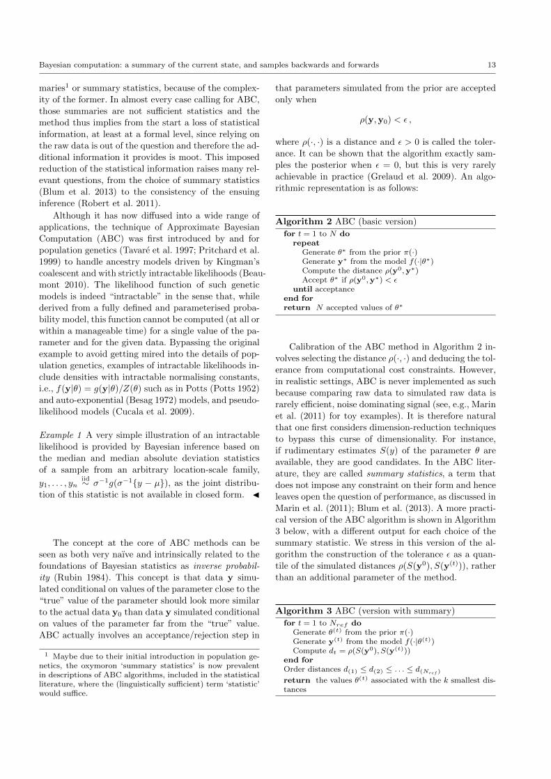
Algorithm 2 ABC (basic version)

for t = 1 to N dorepeat

Generate θ∗ from the prior π(·)Generate y∗ from the model f(·|θ∗)Compute the distance ρ(y0,y∗)Accept θ∗ if ρ(y0,y∗) < ε

until acceptanceend forreturn N accepted values of θ∗

Calibration of the ABC method in Algorithm 2 in-

volves selecting the distance ρ(·, ·) and deducing the tol-

erance from computational cost constraints. However,

in realistic settings, ABC is never implemented as such

because comparing raw data to simulated raw data is

rarely efficient, noise dominating signal (see, e.g., Marin

et al. (2011) for toy examples). It is therefore natural

that one first considers dimension-reduction techniques

to bypass this curse of dimensionality. For instance,

if rudimentary estimates S(y) of the parameter θ are

available, they are good candidates. In the ABC liter-

ature, they are called summary statistics, a term that

does not impose any constraint on their form and hence

leaves open the question of performance, as discussed in

Marin et al. (2011); Blum et al. (2013). A more practi-

cal version of the ABC algorithm is shown in Algorithm

3 below, with a different output for each choice of the

summary statistic. We stress in this version of the al-

gorithm the construction of the tolerance ε as a quan-

tile of the simulated distances ρ(S(y0), S(y(t))), rather

than an additional parameter of the method.

Algorithm 3 ABC (version with summary)

for t = 1 to Nref doGenerate θ(t) from the prior π(·)Generate y(t) from the model f(·|θ(t))Compute dt = ρ(S(y0), S(y(t)))

end forOrder distances d(1) ≤ d(2) ≤ . . . ≤ d(Nref )

return the values θ(t) associated with the k smallest dis-tances

14 P. J. Green, K. Latuszynski, M. Pereyra, & C. P. Robert

An immediate question about this approximate al-

gorithm is how much it remains connected with the

original posterior distribution and in case it does not,

where does it draw its legitimacy. A first remark in this

connection is that it constitutes at best a convergent

approximation to the posterior distribution π(θ|S(y0)).

It can easily be seen that ABC generates outcomes from

a genuine posterior distribution when the data is ran-

domised with scale ε (Wilkinson 2013; Fearnhead and

Prangle 2012). This interpretation indicates a decrease

in the precision of the inference but it does not provide

a universal validation of the method. A second perspec-

tive on the ABC output is that it is based on a non-

parametric approximation of the sampling distribution

(Blum 2010; Blum and Francois 2010), connected with

both indirect inference (Drovandi et al. 2011) and k-

nearest neighbour estimation (Biau et al. 2014). While

a purely Bayesian nonparametric analysis of this aspect

has not yet emerged, this brings an additional if cau-

tious support for the method.

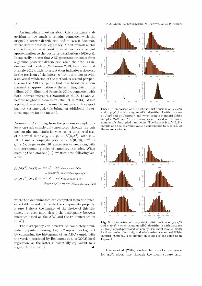
Example 2 Continuing from the previous example of a

location-scale sample only monitored through the pair

median plus mad statistic, we consider the special case

of a normal sample y1, . . . , yn ∼ N (µ, σ2), with n =

100. Using a conjugate prior µ ∼ N (0, 10), σ−2 ∼Ga(2, 5), we generated 106 parameter values, along with

the corresponding pairs of summary statistics. When

creating the distance ρ(·, ·), we used both following ver-

sions:

ρ1(S(y0), S(y)) = |med(y0)−med(y|/mad(med(Y))

+ |mad(y0)−mad(y|/mad(mad(Y))

ρ2(S(y0), S(y)) = |med(y0)−med(y|/mad(med(Y))+

| log mad(y0)−log mad(y|/mad(log mad(Y))

where the denominators are computed from the refer-

ence table in order to scale the components properly.

Figure 1 shows the impact of the choice of this dis-

tance, but even more clearly the discrepancy between

inference based on the ABC and the true inference on

(µ, σ2).

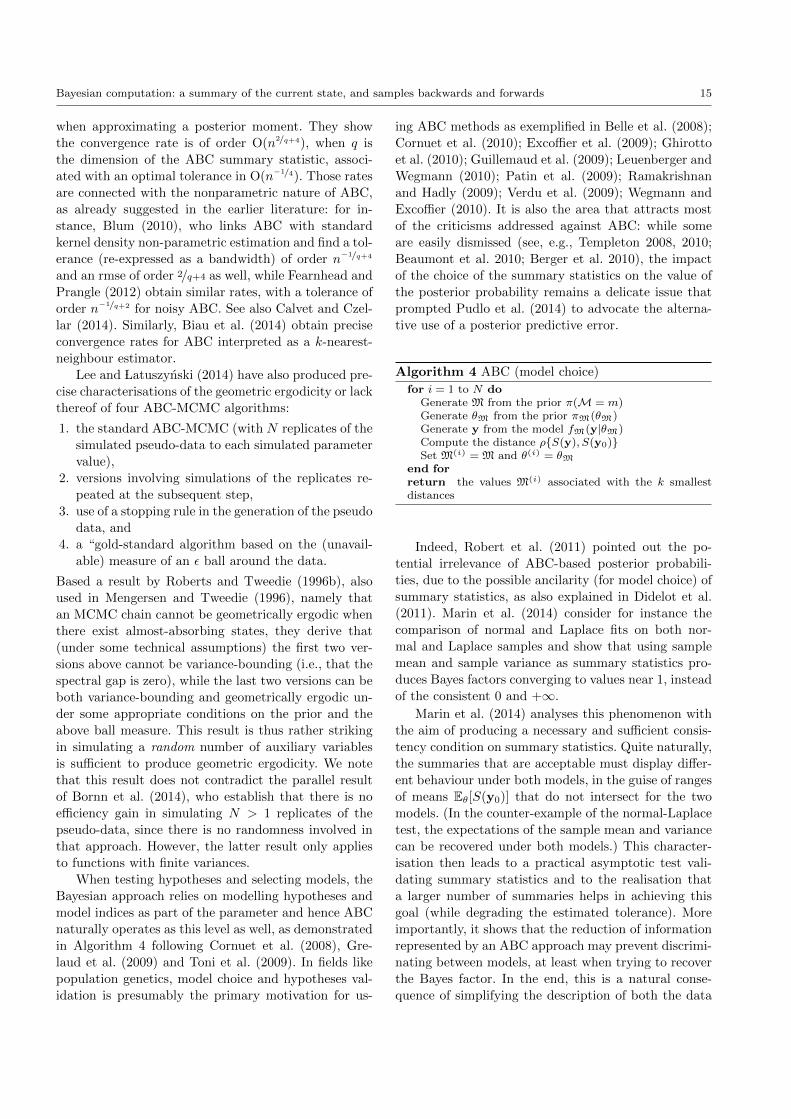
The discrepancy can however be completely elimi-

nated by post-processing: Figure 2 reproduces Figure 1

by comparing the histograms of an ABC sample with

the version corrected by Beaumont et al.’s (2002) local

regression, as the latter is essentially equivalent to a

regular Gibbs output. J

µ

Den

sity

−20 −10 0 10 20

0.00

0.02

0.04

σ

Den

sity

1.0 1.5 2.0 2.5 3.0 3.5

0.0

0.4

0.8

1.2

µ

Den

sity

−20 −10 0 10 20

0.00

0.04

0.08

σ

Den

sity

1.0 1.5 2.0 2.5 3.0 3.5

0.0

0.2

0.4

0.6

0.8

1.0

1.2

µ

Den

sity

−20 −10 0 10 20

0.0

0.5

1.0

1.5

2.0

σ

Den

sity

1.0 1.5 2.0 2.5 3.0 3.5

0.0

0.5

1.0

1.5

2.0

2.5

3.0

Fig. 1 Comparison of the posterior distributions on µ (left)and σ (right) when using an ABC algorithm 3 with distanceρ1 (top) and ρ2 (central), and when using a standard Gibbssampler (bottom). All three samples are based on the samenumber of subsampled parameters. The dataset is a N (3, 22)sample and the tolerance value ε corresponds to α = .5% ofthe reference table.

µ

Den

sity

−30 −20 −10 0 10 20 30

0.00

0.02

0.04

0.06

igmau

Den

sity

1.0 1.5 2.0 2.5

0.0

0.5

1.0

1.5

2.0

µ

Den

sity

2.85 2.90 2.95 3.00 3.05

02

46

810

12

igmau

Den

sity

1.90 1.95 2.00 2.05

05

1015

µ

Den

sity

2.90 2.95 3.00 3.05

02

46

810

12

igmau

Den

sity

1.94 1.96 1.98 2.00 2.02 2.04 2.06

05

1015

20

Fig. 2 Comparison of the posterior distributions on µ (left)and σ (right) when using an ABC algorithm 3 with distanceρ1 (top), a post-processed version by Beaumont et al.’s (2002)local regression (central), and when using a standard Gibbssampler (bottom). The simulation setting is the same as inFigure 1.

Barber et al. (2015) studies the rate of convergence

for ABC algorithms through the mean square error

Bayesian computation: a summary of the current state, and samples backwards and forwards 15

when approximating a posterior moment. They show

the convergence rate is of order O(n2/q+4), when q is

the dimension of the ABC summary statistic, associ-

ated with an optimal tolerance in O(n−1/4). Those rates

are connected with the nonparametric nature of ABC,

as already suggested in the earlier literature: for in-

stance, Blum (2010), who links ABC with standard

kernel density non-parametric estimation and find a tol-

erance (re-expressed as a bandwidth) of order n−1/q+4

and an rmse of order 2/q+4 as well, while Fearnhead and

Prangle (2012) obtain similar rates, with a tolerance of

order n−1/q+2 for noisy ABC. See also Calvet and Czel-

lar (2014). Similarly, Biau et al. (2014) obtain precise

convergence rates for ABC interpreted as a k-nearest-

neighbour estimator.

Lee and Latuszynski (2014) have also produced pre-

cise characterisations of the geometric ergodicity or lack

thereof of four ABC-MCMC algorithms:

1. the standard ABC-MCMC (with N replicates of the

simulated pseudo-data to each simulated parameter

value),

2. versions involving simulations of the replicates re-

peated at the subsequent step,

3. use of a stopping rule in the generation of the pseudo

data, and

4. a “gold-standard algorithm based on the (unavail-

able) measure of an ε ball around the data.

Based a result by Roberts and Tweedie (1996b), also

used in Mengersen and Tweedie (1996), namely that

an MCMC chain cannot be geometrically ergodic when

there exist almost-absorbing states, they derive that

(under some technical assumptions) the first two ver-

sions above cannot be variance-bounding (i.e., that thespectral gap is zero), while the last two versions can be

both variance-bounding and geometrically ergodic un-

der some appropriate conditions on the prior and the

above ball measure. This result is thus rather striking

in simulating a random number of auxiliary variables

is sufficient to produce geometric ergodicity. We note

that this result does not contradict the parallel result

of Bornn et al. (2014), who establish that there is no

efficiency gain in simulating N > 1 replicates of the

pseudo-data, since there is no randomness involved in

that approach. However, the latter result only applies

to functions with finite variances.

When testing hypotheses and selecting models, the

Bayesian approach relies on modelling hypotheses and

model indices as part of the parameter and hence ABC

naturally operates as this level as well, as demonstrated

in Algorithm 4 following Cornuet et al. (2008), Gre-

laud et al. (2009) and Toni et al. (2009). In fields like

population genetics, model choice and hypotheses val-

idation is presumably the primary motivation for us-

ing ABC methods as exemplified in Belle et al. (2008);

Cornuet et al. (2010); Excoffier et al. (2009); Ghirotto

et al. (2010); Guillemaud et al. (2009); Leuenberger and

Wegmann (2010); Patin et al. (2009); Ramakrishnan

and Hadly (2009); Verdu et al. (2009); Wegmann and

Excoffier (2010). It is also the area that attracts most

of the criticisms addressed against ABC: while some

are easily dismissed (see, e.g., Templeton 2008, 2010;

Beaumont et al. 2010; Berger et al. 2010), the impact

of the choice of the summary statistics on the value of

the posterior probability remains a delicate issue that

prompted Pudlo et al. (2014) to advocate the alterna-

tive use of a posterior predictive error.

Algorithm 4 ABC (model choice)

for i = 1 to N doGenerate M from the prior π(M = m)Generate θM from the prior πM(θM)Generate y from the model fM(y|θM)Compute the distance ρ{S(y), S(y0)}Set M(i) = M and θ(i) = θM

end forreturn the values M(i) associated with the k smallestdistances

Indeed, Robert et al. (2011) pointed out the po-

tential irrelevance of ABC-based posterior probabili-

ties, due to the possible ancilarity (for model choice) of

summary statistics, as also explained in Didelot et al.

(2011). Marin et al. (2014) consider for instance the

comparison of normal and Laplace fits on both nor-

mal and Laplace samples and show that using sample

mean and sample variance as summary statistics pro-

duces Bayes factors converging to values near 1, instead

of the consistent 0 and +∞.

Marin et al. (2014) analyses this phenomenon with

the aim of producing a necessary and sufficient consis-

tency condition on summary statistics. Quite naturally,

the summaries that are acceptable must display differ-

ent behaviour under both models, in the guise of ranges

of means Eθ[S(y0)] that do not intersect for the two

models. (In the counter-example of the normal-Laplace

test, the expectations of the sample mean and variance

can be recovered under both models.) This character-

isation then leads to a practical asymptotic test vali-

dating summary statistics and to the realisation that

a larger number of summaries helps in achieving this

goal (while degrading the estimated tolerance). More

importantly, it shows that the reduction of information

represented by an ABC approach may prevent discrimi-

nating between models, at least when trying to recover

the Bayes factor. In the end, this is a natural conse-

quence of simplifying the description of both the data

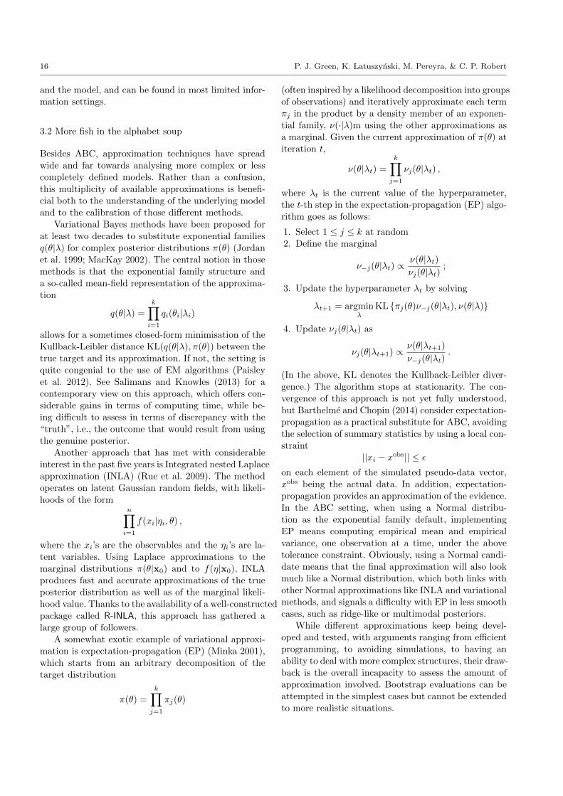
16 P. J. Green, K. Latuszynski, M. Pereyra, & C. P. Robert

and the model, and can be found in most limited infor-

mation settings.

3.2 More fish in the alphabet soup

Besides ABC, approximation techniques have spread

wide and far towards analysing more complex or less

completely defined models. Rather than a confusion,

this multiplicity of available approximations is benefi-

cial both to the understanding of the underlying model

and to the calibration of those different methods.

Variational Bayes methods have been proposed for

at least two decades to substitute exponential families

q(θ|λ) for complex posterior distributions π(θ) (Jordan

et al. 1999; MacKay 2002). The central notion in those

methods is that the exponential family structure and

a so-called mean-field representation of the approxima-

tion

q(θ|λ) =

k∏i=1

qi(θi|λi)

allows for a sometimes closed-form minimisation of the

Kullback-Leibler distance KL(q(θ|λ), π(θ)) between the

true target and its approximation. If not, the setting is

quite congenial to the use of EM algorithms (Paisley

et al. 2012). See Salimans and Knowles (2013) for a

contemporary view on this approach, which offers con-

siderable gains in terms of computing time, while be-

ing difficult to assess in terms of discrepancy with the

“truth”, i.e., the outcome that would result from using

the genuine posterior.

Another approach that has met with considerable

interest in the past five years is Integrated nested Laplace

approximation (INLA) (Rue et al. 2009). The method

operates on latent Gaussian random fields, with likeli-

hoods of the formn∏i=1

f(xi|ηi, θ) ,

where the xi’s are the observables and the ηi’s are la-

tent variables. Using Laplace approximations to the

marginal distributions π(θ|x0) and to f(η|x0), INLA

produces fast and accurate approximations of the true

posterior distribution as well as of the marginal likeli-

hood value. Thanks to the availability of a well-constructed

package called R-INLA, this approach has gathered a

large group of followers.

A somewhat exotic example of variational approxi-

mation is expectation-propagation (EP) (Minka 2001),

which starts from an arbitrary decomposition of the

target distribution

π(θ) =

k∏j=1

πj(θ)

(often inspired by a likelihood decomposition into groups

of observations) and iteratively approximate each term

πj in the product by a density member of an exponen-

tial family, ν(·|λ)m using the other approximations as

a marginal. Given the current approximation of π(θ) at

iteration t,

ν(θ|λt) =

k∏j=1

νj(θ|λt) ,

where λt is the current value of the hyperparameter,

the t-th step in the expectation-propagation (EP) algo-

rithm goes as follows:

1. Select 1 ≤ j ≤ k at random

2. Define the marginal

ν−j(θ|λt) ∝ν(θ|λt)νj(θ|λt)

;

3. Update the hyperparameter λt by solving

λt+1 = argminλ

KL {πj(θ)ν−j(θ|λt), ν(θ|λ)}

4. Update νj(θ|λt) as

νj(θ|λt+1) ∝ ν(θ|λt+1)

ν−j(θ|λt).

(In the above, KL denotes the Kullback-Leibler diver-

gence.) The algorithm stops at stationarity. The con-

vergence of this approach is not yet fully understood,

but Barthelme and Chopin (2014) consider expectation-

propagation as a practical substitute for ABC, avoiding

the selection of summary statistics by using a local con-

straint

||xi − xobs|| ≤ εon each element of the simulated pseudo-data vector,xobs being the actual data. In addition, expectation-

propagation provides an approximation of the evidence.

In the ABC setting, when using a Normal distribu-

tion as the exponential family default, implementing

EP means computing empirical mean and empirical

variance, one observation at a time, under the above

tolerance constraint. Obviously, using a Normal candi-

date means that the final approximation will also look

much like a Normal distribution, which both links with

other Normal approximations like INLA and variational

methods, and signals a difficulty with EP in less smooth

cases, such as ridge-like or multimodal posteriors.

While different approximations keep being devel-

oped and tested, with arguments ranging from efficient

programming, to avoiding simulations, to having an

ability to deal with more complex structures, their draw-

back is the overall incapacity to assess the amount of

approximation involved. Bootstrap evaluations can be

attempted in the simplest cases but cannot be extended

to more realistic situations.

Bayesian computation: a summary of the current state, and samples backwards and forwards 17

4 Optimisation in modern Bayesian

computation

Optimisation methodology for high-dimensional maxi-

mum-a-posteriori (MAP) estimation is another area of

Bayesian computation that has received a lot of atten-

tion over the last years, particularly for problems re-

lated to machine learning, signal processing and com-

puter vision. One reason for this is that for many Bayesian

models optimisation is significantly more computation-

ally tractable than integration. This has generated a

lot of interest in MAP estimators, especially for ap-

plications involving very high-dimensional parameter

spaces or tight computing time constraints, for which

calculating other summaries of the posterior distribu-

tion is not feasible. Here we review some of the major

breakthroughs in this topic, which originated mainly

outside the statistics community. We focus on devel-

opments related to high-dimensional convex optimisa-

tion, though many of the techniques discussed below are

also useful for non-convex optimisation. In particular,

in Section 4.1 we concentrate on proximal optimisation

algorithms, a powerful class of iterative methods that

exploit tools from convex analysis, monotone operator

theory and theory of non-expansive mappings to con-

struct carefully designed fixed-point schemes. We refer

the reader to the excellent book by Bauschke and Com-

bettes (2011) for the mathematics underpinning proxi-

mal optimisation algorithms, and to the recent tutorial

papers by Combettes and Pesquet (2011), Cevher et al.

(2014) and Parikh and Boyd (2014) for an overview of

the field and applications to signal processing and ma-

chine learning.

However, we do think it is vital to insist that, at

the same time as asserting that modern optimisation

methodology represents a much-underused opportunity

in Bayesian inference, in its raw form it inevitably fails

to deliver essential elements of the Bayesian paradigm.

The vision is not to deliver a point estimate of an un-

known structure, but the full richness of Bayesian in-

ference in its coherence, its proper treatment of uncer-

tainty, its intrinsic treatment of model uncertainty, and

so on. Bayesian statistics does not boil down to optimi-

sation with penalisation (Lange et al. 2014). We need

to express the uncertainty associated with decisions and

estimation, stemming from the stochastic nature of the

data, and our lack of knowledge about relevant mecha-

nisms.

The challenge is to use the awesome capacity of fast

optimisation in a high-dimensional parameter space to

focus on local regions of that space where a combina-

tion of analytic and numerical investigation can deliver

at least approximations to full posterior distributions

and derived quantities. The community has barely risen

to this challenge, with only isolated examples such as

the discussion in Green (2015) of a problem in unla-

belled shape analysis. However, the growing community

of INLA (Rue et al. 2009) users may bring an height-

ened awareness of such possibilities, along with its effi-

cient code (Schrodle and Held 2011; Muff et al. 2013).

Another promising research area is to use mathematical

and algorithmic tools from convex optimisation to de-

sign more efficient high-dimensional MCMC algorithms

(Pereyra 2015).

4.1 Proximal algorithms

Similarly to many other computational methodologies

that are widely used nowadays, proximal algorithms

were first proposed several decades ago by Moreau (1962),

Martinet (1970) and Rockafellar (1976), and regained

attention recently in the context of large-scale inverse

problems and “big data”.

We consider the computation of maximisers of pos-

terior densities π(θ) = exp {−g(θ)}/κ that are high-

dimensional and log-concave, which we formulate as

θMAP = argminθ∈Rn

g(θ) (8)

where g belongs to the class Γ0(Rn) of lower semicon-

tinuous convex functions from Rn → (−∞,+∞]. No-

tice that g may be non-differentiable and take value

g(θ) = +∞, reflecting constraints in the parameter

space. In order to introduce proximal algorithms we

first recall the following standard definitions and results

from convex analysis: We say that ϕ ∈ Rn is a subgra-

dient of g at θ ∈ Rn if it satisfies (u − θ)Tϕ + g(θ) ≤g(u),∀u ∈ Rn. The set of all such subgradients defines

the subdifferential set ∂g(θ), and θMAP is a minimiser

of g if and only if 0 ∈ ∂g(θMAP ). The (convex) conju-

gate of g ∈ Γ0(Rn) is the function g∗ ∈ Γ0(Rn) defined

as g∗(ϕ) = supu∈Rn uTϕ− g(u). The subgradients of g

and g∗ satisfy the property ϕ ∈ ∂g(θ)⇔ θ ∈ ∂g∗(ϕ).

Proximal algorithms take their name from the prox-

imity mapping, defined for g ∈ Γ0(Rn) and λ > 0 as

(Moreau 1962)

proxλg (θ) = argminu∈Rn

g(u) + ‖u− θ‖2/2λ. (9)

In order to gain intuition about this mapping it is use-

ful to analyse its behaviour when λ ∈ R+ is either very

small or very large. In the limit λ→∞, the quadratic

penalty term vanishes and (9) maps all points to θMAP .

In the opposite limit λ → 0, (9) becomes the iden-

tity operator and maps θ to itself. For finite values of

λ, proxλg (θ) behaves similarly to a gradient mapping

18 P. J. Green, K. Latuszynski, M. Pereyra, & C. P. Robert

and moves points in the direction of θMAP . Like gradi-

ents, proximity mappings have several properties that

are useful for devising fixed-point methods (Bauschke

and Combettes 2011).

Property 1: The proximity mapping of g is related to

its subdifferential by the inclusion {θ − proxλg (θ)}/λ ∈∂g{proxλg (θ)}, which collapses to ∇g{proxλg (θ)} when

g ∈ C1. As a result, for any λ > 0, the minimiser of g

verifies the fixed-point equation θ = proxλg (θ).

Property 2: Proximity mappings are firmly non-expansive;

that is, ‖ proxλg (θ)−proxλg (u)‖2 ≤ (θ−u)T {proxλg (θ)−proxλg (u)},∀θ,u ∈ Rn.

Property 3: The proximity mappings of g and its con-

jugate g∗ are related by Moreau’s decomposition for-

mula: θ = proxλg (θ) + λprox1/λg∗ (θ/λ).

The simplest proximal method to solve (8) is the

proximal point algorithm given by the iteration

θk+1 = proxλg (θk). (10)

Every sequence {θk}k∈N produced by this algorithm

converges to θMAP , even if proximity mappings are

evaluated inexactly, as long as the errors are of cer-

tain types (e.g., summable). A more general proximal

point algorithm includes relaxation, i.e.,

θk+1 = (1− αk)θk + αk proxλg (θk), αk ∈ (0, 2),

and with over-relaxation (i.e., αk ∈ (1, 2)) often con-

verges faster than (10). Notice from Property 1 that

(10) can be interpreted as an implicit (backward) sub-

gradient steepest descent to minimise g, i.e., θk+1 =

θk − λϕ, with ϕ ∈ ∂g(θk+1

). Alternatively, proximal

point algorithms can also be interpreted as explicit (for-

ward) gradient steepest descent to minimise the Moreau

envelope of g, eλ(θ) = infu∈Rn g(u) + ‖u − θ‖2/2λ, a

convex lower bound on g that by construction is con-

tinuously differentiable and has the same minimiser as

g.

Proximal point algorithms may appear of little rel-

evance because evaluating proxλg can be as difficult as

solving (8) in the first place (notice that (9) is a con-

vex minimisation problem similar to (8)). Surprisingly,

many advanced proximal optimisation methods can in

fact be shown to be either applications of this simple

algorithm, or closely related to it.

Most proximal methods operate by splitting g, e.g.,

θMAP = argminθ∈Rn

{g1(θ) + g2(θ)}, (11)

such that g1 ∈ Γ0(Rn) and g2 ∈ Γ0(Rn) have gra-

dients or proximity mappings that are easy to com-

pute or approximate. For example, for many Bayesian

models it is possible to find a decomposition g(θ) =

g1(θ) + g2(θ) such that g1 is β-Lipschitz2 differentiable

and g2 ∈ Γ0(Rn), possibly non-differentiable, has a

proximity mapping that can be computed efficiently

with a specialised algorithm. This decomposition is use-

ful for instance in linear inverse problems, where g1 is

often related to a Gaussian observation model involv-

ing linear operators and g2 to a log-prior promoting a

parsimonious representation (e.g., sparsity on some ap-

propriate dictionary, low-rankness) or enforcing convex

constraints (e.g., positivity, positive definiteness). For

models that admit this decomposition, it is possible to

compute θMAP efficiently with a forward-backward al-

gorithm, also known as the proximal gradient algorithm

θk+1 = proxλng2 (θk − λn∇g1(θk)). (12)

For λn = λ ∈ (0, 1/β) the objective function g(θk)

converges to g(θMAP ) with rate O(1/k). If the value of

the Lipschitz constant β is unknown λn can be found

by line-search.

A remarkable property of (12) is that it can be accel-

erated to converge with rate O(1/k2), which is optimal

for this class of problems (Nesterov 2004). This can be

achieved for instance by introducing an extrapolation

step

θ+ = θk + ωk(θk − θk−1),

θk+1 = proxβ−1

g2 (θ+ − β−1∇g1(θ+)),(13)

where {ωk}k∈N is an appropriate sequence of extrap-

olation parameters. It was noticed by Combettes and

Pesquet (2011) that several important convex optimi-

sation algorithms can be derived as applications of the

forward-backward algorithm, for example the projected

gradient algorithm for minimising a Lipschitz differen-

tiable function subject to a convex constraint (in this

case the proximity mapping reduces to a projection

onto the convex set). Notice that (12) can be inter-

preted as an implementation of the proximal point iter-

ation (10) where proxλg (θk) is approximated by replac-

ing g1 with its first order Taylor series approximation

around the point θk.

Moreover, in some cases it may be more efficient

to compute θMAP by solving the dual of (11), for in-

stance if g admits a decomposition g(θ) = g1(θ) +

g2(Lθ) for some linear operator L ∈ Rn×p, g1 ∈ Γ0(Rn)

strongly convex and g2 ∈ Γ0(Rp) with efficient proxim-

ity mapping. In this case, the Fenchel–Rockafellar the-

orem states that θMAP can be computed by solving the

2 g1 ∈ C1 has β-Lipschitz continuous gradient if ‖∇g1(θ)−∇g1(u)‖ ≤ β‖θ − u‖, ∀(θ,u) ∈ RN × RN

Bayesian computation: a summary of the current state, and samples backwards and forwards 19

dual problem (Bauschke and Combettes 2011, ch. 19)

ψ∗ = argminψ∈Rp

g∗1(−LTψ) + g∗2(ψ) (14)

and setting θMAP = ∇g∗1(−LTψ∗). This p-dimensional

problem can be solved iteratively with a forward-backward

algorithm ψk+1 = proxλn

g∗2(ψk − λn∇g∗1(−LTψk)) that

can also be accelerated to converge with rate O(1/k2),

and where we note that the proximity mapping of g∗2 is

typically evaluated by using Property 3, and that the

strong convexity of g1 implies Lipschitz differentiability

of g∗1 . Computing θMAP via (14) can lead to important

computational savings, in particular if p � n or if g2

is separable and has a proximity mapping that can be

computed in parallel for each element of θ (this is gen-

erally not possible for g2 ◦ L). We refer the reader to

Komodakis and Pesquet (2014) for an overview of re-

cent dual and primal-dual algorithms and guidelines for

parallel implementations.

Another important proximal optimisation method

is the Douglas–Rachford splitting algorithm given by

θk+ 12 = proxλg1(θk),

θk+1 = θk − θk+ 12 + proxλg2(2θk+ 1

2 − θk).(15)

From a theoretical viewpoint this algorithm is more

general than the forward-backward algorithm because

it does not require g1 or g2 to be continuously differen-

tiable. However, its practical application is limited to

problems for which both g1 and g2 have efficient prox-

imity mappings. Similarly to the forward-backward al-

gorithm, (15) includes many proximal algorithms that

been proposed in the literature for specific models, and

can also be interpreted as an application of the proxi-

mal point algorithm.

The proximal method that is arguably most widely

used in Bayesian inference is the alternating direction

method of multipliers (ADMM), which operates by for-

mulating (11) as a constrained optimisation problem

argminθ∈Rn, z∈Rn

g1(θ) + g2(z)

subject to θ = z,(16)

and then using augmented Langrangian techniques to

express (16) as an unconstrained saddle point problem

with saddle function g1(θ) + g2(z) +λϕT (θ−z) + ||θ−z||2/2λ (Boyd et al. 2011). ADMM solves this problem

with the iteration

θk+1 = proxλg1(zk −ϕk),

zk+1 = proxλg2(θk+1 +ϕk),

ϕk+1 = ϕk + θk+1 − zk+1,

(17)

that also involves the proximity mappings of g1 and g2.

This basic ADMM iteration can be tailored to specific

models in many ways (e.g., to exploit decompositions of

the form g1 = g1 ◦L1 and g2 = g2 ◦L2 so that proximal

updates can be performed in parallel for all components

of θ, z and ϕ). Interestingly, ADMM can be interpreted

as an application of the Douglas–Rachford algorithm to

the dual of (16), and is therefore also a special case of

the proximal point algorithm. For more details about

the ADMM algorithm, see the recent tutorial by Boyd

et al. (2011).

Furthermore, an important characteristic of proxi-

mal optimisation algorithms is that they can be mas-

sively parallelised to take advantage of parallel com-

puter architectures. Suppose for instance that g ad-

mits the decomposition g(θ) =∑Mm=1 gm(Lmθ) with

gm ∈ Γ (Rpm) and Lm ∈ Rn×pm such that the mappings

of gm are easy to compute and Q =∑Mm=1 L

TmLm is in-

vertible. Then, in a manner akin to (16), we express (8)

as

argminz1∈Rn,..., zM∈Rn

∑M

m=1gm(zm)

subject to zm = Lmθ, ∀m = 1, . . . ,M,

(18)

and compute θMAP with the following iteration

θk+1 = Q−1∑M

m=1LTm(zkm −ϕkm),

zk+1m = proxλgm(Lmθ

k+1 −ϕkm), ∀m = 1, . . . ,M,

ϕk+1m = ϕkm + Lmθ

k+1 − zk+1m , ∀m = 1, . . . ,M,

(19)

that can be parallelised with factor M at a coarse level

(e.g., on a multi-processor system). Further parallelisa-

tion may be possible at a finer scale (e.g., on a vectorial

processor such as GPU or FPGA) by taking advantage

of the structure of proxλgm or by using specialised al-

gorithms. This algorithm, known as the simultaneous

direction method of multipliers, is also closely related

to the ADMM, Douglas–Rachford and proximal point

algorithms. Notice that splitting g not only allows the

exploitation of parallel computer architectures, but may

also significantly simplify the computation of proximity

mappings; often proxλgm has a closed-form expression.

Lastly, it is worth mentioning that there are other mod-

ern proximal optimisation algorithms that can be mas-

sively parallelised, for example the generalised forward

backward algorithm (Raguet et al. 2013), the paral-

lel proximal algorithms (Combettes and Pesquet 2008;

Pesquet and Pustelnik 2012), and the parallel primal-

dual algorithm (Combettes and Pesquet 2012).

Finally, main current topics of research in proximal

optimisation include theory and methodology for: 1)

randomised and stochastic algorithms that operate with

20 P. J. Green, K. Latuszynski, M. Pereyra, & C. P. Robert

estimators of gradients and proximity mappings to re-

duce computational complexity and allow for errors in

the update rules, 2) adaptive and variable metric algo-

rithms (e.g. Riemannian and Newton-type) that exploit

the model’s geometry to improve convergence speed,

and 3) proximal methods for non-convex problems. We

anticipate that in the future new and stronger connec-

tions will emerge between proximal optimisation and

stochastic simulation, in particular through develop-

ments in stochastic optimisation and high-dimensional

MCMC sampling. For example, one connection is through

the integration of modern stochastic convex optimisa-

tion and Markovian stochastic approximation (Com-

bettes and Pesquet 2014; Andrieu et al. 2015), and

of proximal optimisation and high-dimensional MCMC

sampling (Pereyra 2015).

4.2 Convex relaxations

Modern proximal optimisation was greatly motivated

by important theoretical results on the recovery of partially-

observed sparse vectors and low-rank matrices through

convex minimisation (Candes et al. 2006; Candes and

Tao 2009) and on compressive sensing (Candes and

Wakin 2008). A key idea underlying these works is that

of approximating a combinatorial optimisation prob-

lem, whose solution is NP-hard, with a “relaxed” con-

vex problem that is computationally tractable, and whose

solution is in some sense close to the solution of the orig-

inal problem. Reciprocally, the development of mod-

ern convex optimisation has in turn generated much

interest in log-concave models, convex regularisers, and“convexifications” (i.e., convex relaxations for intractable

or poorly tractable models) for statistical inference prob-

lems involving high-dimensionality, large datasets and

computing time constraints (Chandrasekaran et al. 2012;

Chandrasekaran and Jordan 2013).

4.3 Illustrative example

For illustration, we show an application of proximal op-

timisation to Bayesian image resolution enhancement.

The goal is to recover a high-resolution image θ ∈ Rnfrom a blurred and noisy observed image y ∼ N (Hθ,

σ2In), where H ∈ Rn×n is a linear operator represent-

ing the blur point spread function of the low resolu-

tion acquisition system and σ2 is the system’s noise

power. This inverse problem is ill-posed, a difficulty that

Bayesian image processing methods address by exploit-

ing prior knowledge about θ. Here we use the following

hierarchical Bayesian model (Oliveira et al. 2009)

f(y|θ) = (2πσ2)−n/2 exp{−‖y −Hθ‖22/2σ2},π(θ|α) ∝ α−n exp (−α‖∇dθ‖1−2),

π(α) = e−α1R+(α),

(20)

where π(θ|α) is the (improper) total-variation Markov

random field, ‖·‖1−2 denotes the composite `1−`2 norm

and ∇d is the discrete gradient operator that computes

the vertical and horizontal differences between neigh-

bour image pixels. This prior is log-concave and mod-

els the fact that differences between neighbouring im-

age pixels are usually very small but occasionally take

large values; it is arguably the most widely used prior

in modern statistical image processing. The values of

H and σ2 are typically determined during the system’s

calibration process and are here assumed known.

We compute the MAP estimator of θ associated

with the marginal posterior π(θ|y) =∫∞

0π(θ, α|y)dα,

which is unimodal but not log-concave,

θMAP = argminθ∈Rn

‖y −Hθ‖22/2σ2

+ (n+ 1) log (‖∇dθ‖1−2 + 1) .(21)

Problem (21) is not convex, but can nevertheless be

solved efficiently with proximal algorithms by using a

majorisation–minimisation strategy. To be precise, start-

ing from some initial condition θ(0), e.g., θ(0) = y, we

iteratively minimise the following sequence of strictly

convex majorants (Oliveira et al. 2009)

θ(t+1) = argminθ∈Rn

‖y −Hθ‖22/2σ2 + α(t)eff ‖∇dθ‖1−2,

with α(t)eff = (n+ 1)(‖∇dθ(t)‖1−2 + 1).

(22)

Iteration (22) involves a convex subproblem that can

easily be solved using most modern proximal optimisa-

tion techniques. For example, here we use the state-of-

the-art ADMM algorithm SALSA (Afonso et al. 2011)

implemented with g1(θ) = ‖y − Hθ‖22/2σ2, g2(u) =

α(t)eff‖∇du‖1−2, and the constraint θ = u [though we

could have also used other modern algorithms (Pes-

quet and Pustelnik 2012; Combettes and Pesquet 2012;

Raguet et al. 2013)]. To compute the proximity map-

ping of g1 we use the fact that H is block-circulant to

compute matrix products and pseudo-inverses with the

FFT algorithm. We compute the proximity mapping

of g2 with a highly parallelised implementation of the

specialised algorithm of Chambolle (2004).

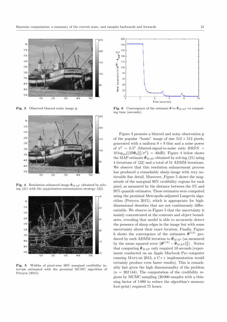
Bayesian computation: a summary of the current state, and samples backwards and forwards 21

Fig. 3 Observed blurred noisy image y.

Fig. 4 Resolution enhanced image θMAP obtained by solv-ing (21) with the majorisation-minimisation strategy (22).

Fig. 5 Widths of pixel-wise 90% marginal credibility in-tervals estimated with the proximal MCMC algorithm ofPereyra (2015).

Fig. 6 Convergence of the estimate θ to θMAP vs comput-ing time (seconds).

Figure 3 presents a blurred and noisy observation y

of the popular “boats” image of size 512 × 512 pixels,

generated with a uniform 9× 9 blur and a noise power

of σ2 = 0.52 (blurred-signal-to-noise ratio BRSN =

10 log10{‖Hθ0‖22/σ2} = 40dB). Figure 4 below shows

the MAP estimate θMAP obtained by solving (21) using

4 iterations of (22) and a total of 51 ADMM iterations.

We observe that this resolution enhancement process

has produced a remarkably sharp image with very no-

ticeable fine detail. Moreover, Figure 5 shows the mag-

nitude of the marginal 90% credibility regions for each

pixel, as measured by the distance between the 5% and

95% quantile estimates. These estimates were computedusing the proximal Metropolis-adjusted Langevin algo-

rithm (Pereyra 2015), which is appropriate for high-

dimensional densities that are not continuously differ-

entiable. We observe in Figure 5 that the uncertainty is

mainly concentrated at the contours and object bound-

aries, revealing that model is able to accurately detect

the presence of sharp edges in the image but with some

uncertainty about their exact location. Finally, Figure

6 shows the convergence of the estimates θ(t,k) pro-

duced by each ADMM iteration to θMAP (as measured

by the mean squared error ‖θ(t,k) − θMAP ‖22) . Notice

that computing θMAP only required 10 seconds (exper-

iment conducted on an Apple Macbook Pro computer

running Matlab 2013, a C++ implementation would

certainly produce even faster results). This is remark-

ably fast given the high dimensionality of the problem

(n = 262 144). The computation of the credibility re-

gions by MCMC sampling (20 000 samples with a thin-

ning factor of 1 000 to reduce the algorithm’s memory

foot-print) required 75 hours.

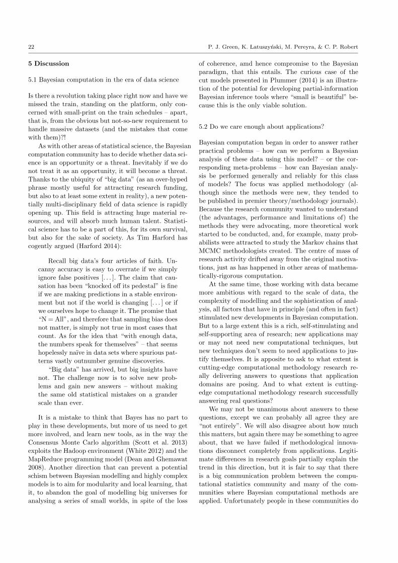
22 P. J. Green, K. Latuszynski, M. Pereyra, & C. P. Robert

5 Discussion

5.1 Bayesian computation in the era of data science

Is there a revolution taking place right now and have we

missed the train, standing on the platform, only con-

cerned with small-print on the train schedules – apart,

that is, from the obvious but not-so-new requirement to

handle massive datasets (and the mistakes that come

with them)?!

As with other areas of statistical science, the Bayesian

computation community has to decide whether data sci-

ence is an opportunity or a threat. Inevitably if we do

not treat it as an opportunity, it will become a threat.

Thanks to the ubiquity of “big data” (as an over-hyped

phrase mostly useful for attracting research funding,

but also to at least some extent in reality), a new poten-

tially multi-disciplinary field of data science is rapidly

opening up. This field is attracting huge material re-

sources, and will absorb much human talent. Statisti-

cal science has to be a part of this, for its own survival,

but also for the sake of society. As Tim Harford has

cogently argued (Harford 2014):

Recall big data’s four articles of faith. Un-

canny accuracy is easy to overrate if we simply

ignore false positives [. . . ]. The claim that cau-

sation has been “knocked off its pedestal” is fine

if we are making predictions in a stable environ-

ment but not if the world is changing [. . . ] or if

we ourselves hope to change it. The promise that

“N = All”, and therefore that sampling bias does

not matter, is simply not true in most cases that

count. As for the idea that “with enough data,

the numbers speak for themselves” – that seems

hopelessly naıve in data sets where spurious pat-

terns vastly outnumber genuine discoveries.

“Big data” has arrived, but big insights have

not. The challenge now is to solve new prob-

lems and gain new answers – without making

the same old statistical mistakes on a grander

scale than ever.

It is a mistake to think that Bayes has no part to

play in these developments, but more of us need to get

more involved, and learn new tools, as in the way the

Consensus Monte Carlo algorithm (Scott et al. 2013)

exploits the Hadoop environment (White 2012) and the

MapReduce programming model (Dean and Ghemawat

2008). Another direction that can prevent a potential

schism between Bayesian modelling and highly complex

models is to aim for modularity and local learning, that

it, to abandon the goal of modelling big universes for

analysing a series of small worlds, in spite of the loss

of coherence, amd hence compromise to the Bayesian

paradigm, that this entails. The curious case of the

cut models presented in Plummer (2014) is an illustra-

tion of the potential for developing partial-information

Bayesian inference tools where “small is beautiful” be-

cause this is the only viable solution.

5.2 Do we care enough about applications?

Bayesian computation began in order to answer rather

practical problems – how can we perform a Bayesian

analysis of these data using this model? – or the cor-

responding meta-problems – how can Bayesian analy-

sis be performed generally and reliably for this class

of models? The focus was applied methodology (al-

though since the methods were new, they tended to

be published in premier theory/methodology journals).

Because the research community wanted to understand

(the advantages, performance and limitations of) the

methods they were advocating, more theoretical work

started to be conducted, and, for example, many prob-

abilists were attracted to study the Markov chains that

MCMC methodologists created. The centre of mass of

research activity drifted away from the original motiva-

tions, just as has happened in other areas of mathema-

tically-rigorous computation.

At the same time, those working with data became

more ambitious with regard to the scale of data, the

complexity of modelling and the sophistication of anal-

ysis, all factors that have in principle (and often in fact)

stimulated new developments in Bayesian computation.

But to a large extent this is a rich, self-stimulating and

self-supporting area of research; new applications may

or may not need new computational techniques, but

new techniques don’t seem to need applications to jus-

tify themselves. It is apposite to ask to what extent is

cutting-edge computational methodology research re-

ally delivering answers to questions that application

domains are posing. And to what extent is cutting-

edge computational methodology research successfully

answering real questions?

We may not be unanimous about answers to these

questions, except we can probably all agree they are

“not entirely”. We will also disagree about how much

this matters, but again there may be something to agree

about, that we have failed if methodological innova-

tions disconnect completely from applications. Legiti-

mate differences in research goals partially explain the

trend in this direction, but it is fair to say that there

is a big communication problem between the compu-

tational statistics community and many of the com-

munities where Bayesian computational methods are

applied. Unfortunately people in these communities do

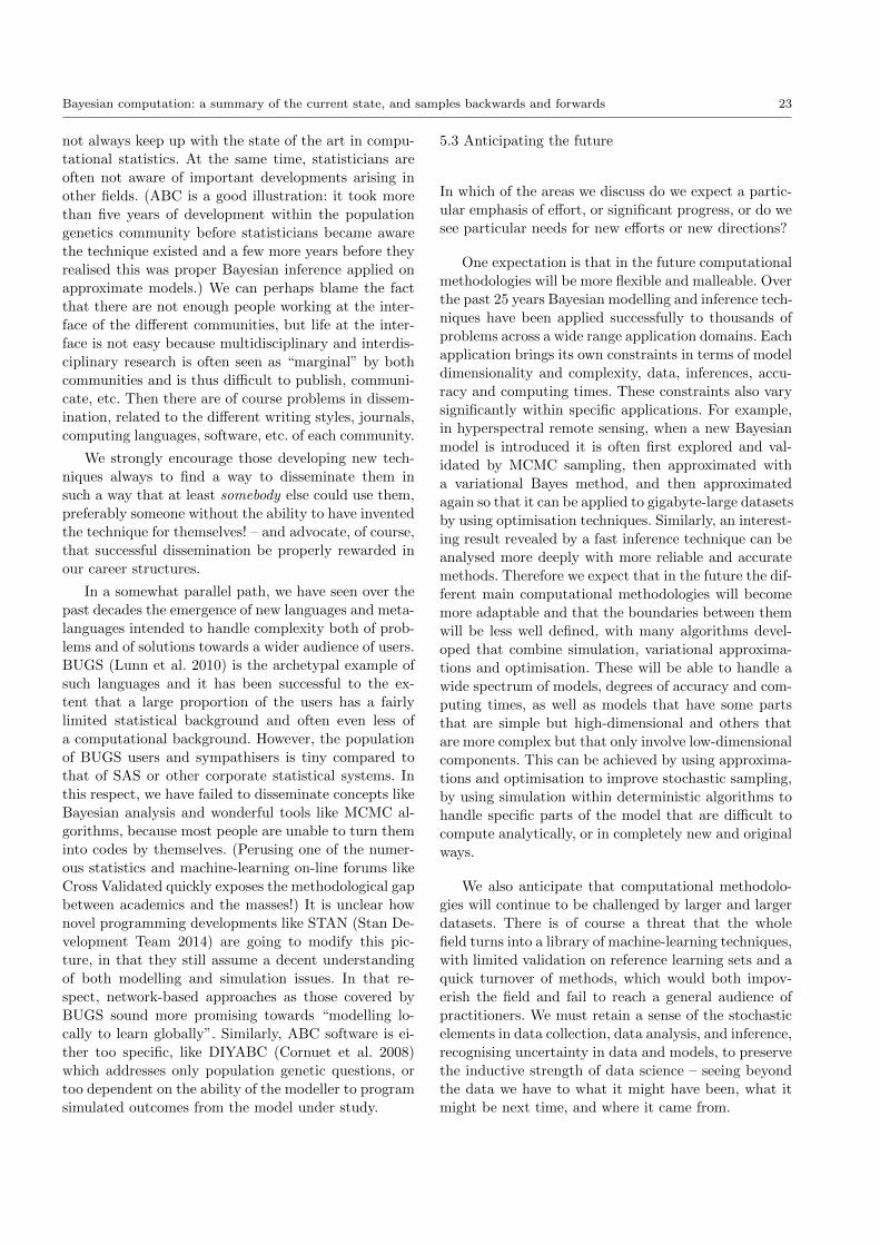
Bayesian computation: a summary of the current state, and samples backwards and forwards 23

not always keep up with the state of the art in compu-

tational statistics. At the same time, statisticians are

often not aware of important developments arising in

other fields. (ABC is a good illustration: it took more

than five years of development within the population

genetics community before statisticians became aware

the technique existed and a few more years before they

realised this was proper Bayesian inference applied on

approximate models.) We can perhaps blame the fact

that there are not enough people working at the inter-

face of the different communities, but life at the inter-

face is not easy because multidisciplinary and interdis-

ciplinary research is often seen as “marginal” by both

communities and is thus difficult to publish, communi-

cate, etc. Then there are of course problems in dissem-

ination, related to the different writing styles, journals,

computing languages, software, etc. of each community.

We strongly encourage those developing new tech-

niques always to find a way to disseminate them in

such a way that at least somebody else could use them,

preferably someone without the ability to have invented

the technique for themselves! – and advocate, of course,

that successful dissemination be properly rewarded in

our career structures.

In a somewhat parallel path, we have seen over the

past decades the emergence of new languages and meta-

languages intended to handle complexity both of prob-

lems and of solutions towards a wider audience of users.

BUGS (Lunn et al. 2010) is the archetypal example of

such languages and it has been successful to the ex-

tent that a large proportion of the users has a fairly

limited statistical background and often even less of

a computational background. However, the populationof BUGS users and sympathisers is tiny compared to

that of SAS or other corporate statistical systems. In

this respect, we have failed to disseminate concepts like

Bayesian analysis and wonderful tools like MCMC al-

gorithms, because most people are unable to turn them

into codes by themselves. (Perusing one of the numer-

ous statistics and machine-learning on-line forums like

Cross Validated quickly exposes the methodological gap

between academics and the masses!) It is unclear how

novel programming developments like STAN (Stan De-

velopment Team 2014) are going to modify this pic-

ture, in that they still assume a decent understanding

of both modelling and simulation issues. In that re-

spect, network-based approaches as those covered by

BUGS sound more promising towards “modelling lo-

cally to learn globally”. Similarly, ABC software is ei-

ther too specific, like DIYABC (Cornuet et al. 2008)

which addresses only population genetic questions, or

too dependent on the ability of the modeller to program

simulated outcomes from the model under study.

5.3 Anticipating the future

In which of the areas we discuss do we expect a partic-

ular emphasis of effort, or significant progress, or do we

see particular needs for new efforts or new directions?

One expectation is that in the future computational

methodologies will be more flexible and malleable. Over

the past 25 years Bayesian modelling and inference tech-

niques have been applied successfully to thousands of

problems across a wide range application domains. Each

application brings its own constraints in terms of model

dimensionality and complexity, data, inferences, accu-

racy and computing times. These constraints also vary

significantly within specific applications. For example,

in hyperspectral remote sensing, when a new Bayesian

model is introduced it is often first explored and val-

idated by MCMC sampling, then approximated with

a variational Bayes method, and then approximated

again so that it can be applied to gigabyte-large datasets

by using optimisation techniques. Similarly, an interest-

ing result revealed by a fast inference technique can be

analysed more deeply with more reliable and accurate

methods. Therefore we expect that in the future the dif-

ferent main computational methodologies will become

more adaptable and that the boundaries between them

will be less well defined, with many algorithms devel-

oped that combine simulation, variational approxima-

tions and optimisation. These will be able to handle a

wide spectrum of models, degrees of accuracy and com-

puting times, as well as models that have some parts

that are simple but high-dimensional and others that

are more complex but that only involve low-dimensional

components. This can be achieved by using approxima-

tions and optimisation to improve stochastic sampling,

by using simulation within deterministic algorithms to

handle specific parts of the model that are difficult to

compute analytically, or in completely new and original

ways.

We also anticipate that computational methodolo-

gies will continue to be challenged by larger and larger

datasets. There is of course a threat that the whole

field turns into a library of machine-learning techniques,

with limited validation on reference learning sets and a

quick turnover of methods, which would both impov-

erish the field and fail to reach a general audience of

practitioners. We must retain a sense of the stochastic

elements in data collection, data analysis, and inference,

recognising uncertainty in data and models, to preserve

the inductive strength of data science – seeing beyond

the data we have to what it might have been, what it

might be next time, and where it came from.

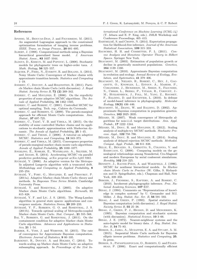
24 P. J. Green, K. Latuszynski, M. Pereyra, & C. P. Robert

References

Afonso, M., Bioucas-Dias, J. and Figueiredo, M. (2011).An augmented Lagrangian approach to the constrainedoptimization formulation of imaging inverse problems.IEEE. Trans. on Image Process., 20 681–695.

Albert, J. (1988). Computational methods using a Bayesianhierarchical generalized linear model. J. AmericanStatist. Assoc., 83 1037–1044.

Aldous, D., Krikun, M. and Popovic, L. (2008). Stochasticmodels for phylogenetic trees on higher-order taxa. J.Math. Biology, 56 525–557.

Alquier, P., Friel, N., Everitt, R. and Boland, A. (2014).Noisy Monte Carlo: Convergence of Markov chains withapproximate transition kernels. Statistics and Computing1–19.

Andrieu, C., Doucet, A. and Holenstein, R. (2011). Parti-cle Markov chain Monte Carlo (with discussion). J. RoyalStatist. Society Series B, 72 (2) 269–342.

Andrieu, C. and Moulines, E. (2006). On the ergodicityproperties of some adaptive MCMC algorithms. The An-nals of Applied Probability, 16 1462–1505.

Andrieu, C. and Robert, C. (2001). Controlled MCMC foroptimal sampling. Tech. rep., Cahiers du Ceremade.

Andrieu, C. and Roberts, G. (2009). The pseudo-marginalapproach for efficient Monte Carlo computations. Ann.Statist., 37 697–725.

Andrieu, C., Tadic, V. B. and Vihola, M. (2015). On thestability of some controlled Markov chains and its appli-cations to stochastic approximation with Markovian dy-namic. The Annals of Applied Probability, 25 1–45.

Andrieu, C. and Thoms, J. (2008). A tutorial on adaptiveMCMC. Statistics and Computing, 18 343–373.

Andrieu, C. and Vihola, M. (2015). Convergence propertiesof pseudo-marginal markov chain monte carlo algorithms.Annals of Applied Probability, 25 1030–1077.

Angelino, E., Kohler, E., Waterland, A., Seltzer, M.and Adams, R. (2014). Accelerating MCMC via parallelpredictive prefetching. arXiv preprint arXiv:1403.7265.

Atchade, Y. (2006). An adaptive version for the Metropo-lis adjusted Langevin algorithm with a truncated drift.Methodology and Computing in Applied Probability, 8235–254.

Atchade, Y., Fort, G., Moulines, E. and Priouret, P.(2011a). Adaptive Markov chain Monte Carlo: theory andmethods. In Bayesian Time Series Models. CambridgeUniversity Press.

Atchade, Y. and Rosenthal, J. (2005). On adaptiveMarkov chain Monte Carlo algorithms. Bernoulli, 11815–828.

Atchade, Y. F. and Liu, J. S. (2010). The Wang-Landaualgorithm in general state spaces: applications and con-vergence analysis. Statistica Sinica, 20 209–233.

Atchade, Y. F., Roberts, G. O. and Rosenthal, J. S.(2011b). Towards optimal scaling of Metropolis-coupledMarkov chain Monte Carlo. Stat. Comput., 21 555–568.

Bai, Y., Roberts, G. and Rosenthal, J. (2011). On thecontainment condition for adaptive Markov chain MonteCarlo algorithms. Advances and Applications in Statis-tics, 21 1–54.

Barber, S., Voss, J. and Webster, M. (2015). The rateof convergence for Approximate Bayesian computation.Electronic Journal of Statistics, 9 80–105.

Bardenet, R., Doucet, A. and Holmes, C. (2014). To-wards scaling up Markov chain Monte Carlo: an adaptivesubsampling approach. In Proceedings of the 31st In-

ternational Conference on Machine Learning (ICML-14)(T. Jebara and E. P. Xing, eds.). JMLR Workshop andConference Proceedings, 405–413.

Barthelme, S. and Chopin, N. (2014). Expectation propaga-tion for likelihood-free inference. Journal of the AmericanStatistical Association, 109 315–333.

Bauschke, H. H. and Combettes, P. L. (2011). Con-vex Analysis and Monotone Operator Theory in HilbertSpaces. Springer New York.

Beaumont, M. (2003). Estimation of population growth ordecline in genetically monitored populations. Genetics,164 1139–1160.

Beaumont, M. (2010). Approximate Bayesian computationin evolution and ecology. Annual Review of Ecology, Evo-lution, and Systematics, 41 379–406.

Beaumont, M., Nielsen, R., Robert, C., Hey, J., Gag-giotti, O., Knowles, L., Estoup, A., Mahesh, P.,Coranders, J., Hickerson, M., Sisson, S., Fagundes,N., Chikhi, L., Beerli, P., Vitalis, R., Cornuet, J.-M., Huelsenbeck, J., Foll, M., Yang, Z., Rousset,F., Balding, D. and Excoffier, L. (2010). In defenseof model-based inference in phylogeography. MolecularEcology, 19(3) 436–446.

Beaumont, M., Zhang, W. and Balding, D. (2002). Ap-proximate Bayesian computation in population genetics.Genetics, 162 2025–2035.

Bedard, M. (2007). Weak convergence of Metropolis al-gorithms for non-i.i.d. target distributions. Ann. Appl.Probab., 17 1222–1244.

Bedard, M., Douc, R. and Moulines, E. (2012). Scalinganalysis of multiple-try MCMC methods. Stochastic Pro-cess. Appl., 122 758–786.

Bedard, M., Douc, R. and Moulines, E. (2014). Scalinganalysis of delayed rejection MCMC methods. Methodol.Comput. Appl. Probab., 16 811–838.

Belle, E., Benazzo, A., Ghirotto, S., Colonna, V. andBarbujani, G. (2008). Comparing models on the ge-nealogical relationships among Neandertal, Cro-Magnoidand modern Europeans by serial coalescent simulations.Heredity, 102 218–225.

Bennett, J., Racine-Poon, A. and Wakefield, J. (1996).MCMC for nonlinear hierarchical models. In Markovchain Monte Carlo in Practice (W. Gilks, S. Richard-son and D. Spiegelhalter, eds.). Chapman and Hall, NewYork, 339–358.

Berger, J., Fienberg, S., Raftery, A. and Robert, C.(2010). Incoherent phylogeographic inference. Proc. Na-tional Academy Sciences, 107 E57.

Besag, J. (1994). Comments on “Representations of knowl-edge in complex systems” by U. Grenander and M.I.Miller. J. Roy. Statist. Soc. Ser. B, 56 591–592.

Besag, J. and Green, P. (1993). Spatial statistics andBayesian computation (with discussion). J. Royal Statist.Society Series B, 55 25–38.

Besag, J., Green, P. J., Higdon, D. and Mengersen, K.(1995). Bayesian computation and stochastic systems(with discussion). Statistical Science, 10 3–66.

Besag, J. E. (1972). Nearest-neighbour systems and theauto-logistic model for binary data. J. Roy. Statist. Soc.Ser. B, 34 75–83.

Beskos, A., Jasra, A., Muzaffer, E. A. and Stuart, A. M.(2015). Sequential Monte Carlo methods for Bayesianelliptic inverse problems. Statistics and Computing, 25.In press.

Beskos, A., Papaspiliopoulos, O., Roberts, G. and Fearn-head, P. (2006). Exact and computationally efficient

Bayesian computation: a summary of the current state, and samples backwards and forwards 25

likelihood-based estimation for discretely observed diffu-sion processes (with discussion). J. Royal Statist. SocietySeries B, 68 333–382.

Beskos, A., Pillai, N., Roberts, G., Sanz-Serna, J.-M.and Stuart, A. (2013). Optimal tuning of the hybridMonte Carlo algorithm. Bernoulli, 19 1501–1534.

Beskos, A., Roberts, G. and Stuart, A. (2009). Optimalscalings for local Metropolis-Hastings chains on nonprod-uct targets in high dimensions. Ann. Appl. Probab., 19863–898.

Betancourt, M. (2013). A general metric for Riemannianmanifold Hamiltonian Monte Carlo. In National Confer-ence on the Geometric Science of Information (F. Nielsenand F. Barbaresco, eds.). Lecture Notes in Computer Sci-ence 8085, Springer, 327–334.

Betancourt, M., Byrne, S. and Girolami, M. (2014). Op-timizing the integrator step size for Hamiltonian MonteCarlo. arXiv preprint arXiv:1411.6669.

Betancourt, M. J., Byrne, S., Livingstone, S. and Giro-lami, M. (2014). The geometric foundations of Hamilto-nian Monte Carlo. ArXiv e-prints. 1410.5110.

Biau, G., Cerou, F. and Guyader, A. (2014). New in-sights into Approximate Bayesian computation. Annalesde l’IHP (Probability and Statistics), 51 376–403.

Blum, M. (2010). Approximate Bayesian computation: anon-parametric perspective. J. American Statist. Assoc.,105 1178–1187.

Blum, M. and Francois, O. (2010). Non-linear regressionmodels for approximate Bayesian computation. Statist.Comput., 20 63–73.

Blum, M., Nunes, M., Prangle, D. and Sisson, S. (2013).A comparative review of dimension reduction methods inApproximate Bayesian computation. Stat Sci, 28 189–208.

Bornn, L., Pillai, N., Smith, A. and Woodard, D. (2014).A pseudo-marginal perspective on the ABC algorithm.ArXiv e-prints. 1404.6298.

Bou-Rabee, N. and Hairer, M. (2012). Nonasymptotic mix-ing of the MALA algorithm. IMA Journal of NumericalAnalysis drs003.

Boyd, S., Parikh, N., Chu, E., Peleato, B. and Eckstein,J. (2011). Distributed optimization and statistical learn-ing via the alternating direction method of multipliers.Found. Trends Mach. Learn., 3 1–122.

Brockwell, A. (2006). Parallel Markov chain Monte Carlosimulation by pre-fetching. J. Comput. Graphical Stat.,15 246–261.

Calderhead, B. (2014). A general construction for paral-lelizing Metropolis–Hastings algorithms. Proceedings ofthe National Academy of Sciences, 111 17408–17413.

Calvet, C. and Czellar, V. (2014). Accurate methods forApproximate Bayesian computation filtering. J. Finan-cial Econometrics. (to appear).

Candes, E. J., Romberg, J. K. and Tao, T. (2006). Stablesignal recovery from incomplete and inaccurate measure-ments. Communications on Pure and Applied Mathemat-ics, 59 1207–1223.

Candes, E. J. and Tao, T. (2009). The power of convex re-laxation: Near-optimal matrix completion. IEEE Trans.Inform. Theory, 56 2053–2080.

Candes, E. J. and Wakin, M. B. (2008). An introductionto compressive sampling. IEEE Signal Process. Mag., 2521–30.

Cappe, O., Robert, C. and Ryden, T. (2002). Reversiblejump MCMC converging to birth-and-death MCMC andmore general continuous time samplers. J. Royal Statist.

Society Series B, 65 679–700.Carlin, B. and Gelfand, A. (1991). An iterative Monte

Carlo method for nonconjugate Bayesian analysis. Statis-tics and Computing, 1 119–28.

Carlin, B., Gelfand, A. and Smith, A. (1992). Hierarchi-cal Bayesian analysis of change point problems. AppliedStatistics (Series C), 41 389–405.

Cevher, V., Becker, S. and Schmidt, M. (2014). Convexoptimization for big data: Scalable, randomized, and par-allel algorithms for big data analytics. Signal ProcessingMagazine, IEEE, 31 32–43.

Chambolle, A. (2004). An algorithm for total variation min-imization and applications. J. Math. Imaging Vis., 2089–97.

Chandrasekaran, V. and Jordan, M. I. (2013). Compu-tational and statistical tradeoffs via convex relaxation.PNAS, 110 1181–1190.

Chandrasekaran, V., Recht, B., Parrilo, P. and Will-sky, A. (2012). The convex geometry of linear inverseproblems. Found. Comput. Math., 12 805–849.

Chipman, H., George, E. and McCulloch, R. (2008).BART: Bayesian additive regression trees. Tech. rep.,Acadia University. ArXiv:0806.3286v1.

Chopin, N. (2007). Inference and model choice for time-ordered hidden Markov models. J. Royal Statist. SocietySeries B, 69(2) 269–284.

Chopin, N., Jacob, P. E. and Papaspiliopoulos, O. (2013).SMC2: an efficient algorithm for sequential analysis ofstate space models. J. Royal Statist. Society Series B,75 397–426.

Christensen, O., Roberts, G. and Rosenthal, J. (2005).Scaling limits for the transient phase of local Metropolis–Hastings algorithms. Journal of the Royal Statistical So-ciety: Series B (Statistical Methodology), 67 253–268.

Combettes, P. L. and Pesquet, J.-C. (2008). A proximaldecomposition method for solving convex variational in-verse problems. Inverse Problems, 24 065014.

Combettes, P. L. and Pesquet, J.-C. (2011). Proximalsplitting methods in signal processing. In Fixed-Point Al-gorithms for Inverse Problems in Science and Engineer-ing (H. H. Bauschke, R. S. Burachik, P. L. Combettes,V. Elser, D. R. Luke and H. Wolkowicz, eds.). SpringerNew York, 185–212.

Combettes, P. L. and Pesquet, J.-C. (2012). Primal-dualsplitting algorithm for solving inclusions with mixtures ofcomposite, Lipschitzian, and parallel-sum type monotoneoperators. Set-Valued A., 20 307–330.

Combettes, P. L. and Pesquet, J.-C. (2014). StochasticQuasi-Fejer block-coordinate fixed point iterations withrandom sweeping. ArXiv e-prints. 1404.7536.

Cornuet, J.-M., Ravigne, V. and Estoup, A. (2010). In-ference on population history and model checking usingDNA sequence and microsatellite data with the softwareDIYABC (v1.0). BMC Bioinformatics, 11 401.

Cornuet, J.-M., Santos, F., Beaumont, M., Robert, C.,Marin, J.-M., Balding, D., Guillemaud, T. and Es-toup, A. (2008). Inferring population history withDIYABC: a user-friendly approach to ApproximateBayesian computation. Bioinformatics, 24 2713–2719.

Cotter, S., Roberts, G., Stuart, A., White, D. et al.(2013). MCMC methods for functions: modifying old al-gorithms to make them faster. Statistical Science, 28424–446.

Craiu, R., Rosenthal, J. and Yang, C. (2009). Learnfrom thy neighbour: Parallel-chain and regional adaptiveMCMC. J. American Statist. Assoc., 104 1454–1466.

26 P. J. Green, K. Latuszynski, M. Pereyra, & C. P. Robert

Craiu, R. V. and Meng, X.-L. (2005). Multiprocess paral-lel antithetic coupling for backward and forward Markovchain Monte Carlo. Ann. Statist., 33 661–697.

Cucala, L., Marin, J.-M., Robert, C. and Titterington,D. (2009). Bayesian inference in k-nearest-neighbour clas-sification models. J. American Statist. Assoc., 104 (485)263–273.

Dean, J. and Ghemawat, S. (2008). MapReduce: simplifieddata processing on large clusters. Communications of theACM, 51 107–113.

Del Moral, P., Doucet, A. and Jasra, A. (2006). Se-quential Monte Carlo samplers. J. Royal Statist. SocietySeries B, 68 411–436.

Dellaportas, P., Papaspiliopoulos, O. and Roberts, G.(2004). Bayesian inference for non-Gaussian Ornstein-uhlenbeck stochastic volatility processes. J. Royal Statist.Society Series B, 66 369–393.

Dellaportas, P. and Wright, D. (1991). Positive embeddedintegration in Bayesian analysis. Statistics and Comput-ing, 1 1–12.

Diaconis, P. and Stroock, D. (1991). Geometric boundsfor eigenvalues of Markov chains. The Annals of AppliedProbability 36–61.

Didelot, X., Everitt, R., Johansen, A. and Lawson, D.(2011). Likelihood-free estimation of model evidence.Bayesian Analysis, 6 48–76.

Diebolt, J. and Robert, C. (1994). Estimation of finite mix-ture distributions by Bayesian sampling. J. Royal Statist.Society Series B, 56 363–375.

Doll, J. and Dion, D. (1976). Generalized Langevin equa-tion approach for atom/solid–surface scattering: Numeri-cal techniques for Gaussian generalized Langevin dynam-ics. The Journal of Chemical Physics, 65 3762–3766.

Douc, R. and Robert, C. (2011). A vanilla Rao–Blackwellization of Metropolis–Hastings algorithms.Ann. Statist., 39 261–277.

Doucet, A., Pitt, M., Deligiannidis, G. and Kohn, R.(2012). Efficient implementation of Markov chain MonteCarlo when using an unbiased likelihood estimator. arXivpreprint arXiv:1210.1871 Biometrika to appear 2015.

Drovandi, C., Pettitt, A. and Fddy, M. (2011). Approx-imate Bayesian computation using indirect inference. J.Royal Statist. Society Series A, 60 503–524.

Duane, S., Kennedy, A. D., Pendleton, B. J., andRoweth, D. (1987). Hybrid Monte Carlo. Phys. Lett.B, 195 216–222.

Ermak, D. (1975). A computer simulation of charged parti-cles in solution. I. Technique and equilibrium properties.The Journal of Chemical Physics, 62 4189–4196.

Excoffier, C., Leuenberger, D. and Wegmann, L. (2009).Bayesian computation and model selection in populationgenetics. ArXiv:0901.2231.

Fearnhead, P. and Clifford, P. (2003). On-line inferencefor hidden Markov models via particle filters. J. RoyalStatist. Society Series B, 65 887–899.

Fearnhead, P. and Prangle, D. (2012). Constructingsummary statistics for Approximate Bayesian compu-tation: semi-automatic Approximate Bayesian computa-tion. Journal of the Royal Statistical Society: SeriesB (Statistical Methodology), 74 419–474. (With discus-sion.).

Fort, G., Moulines, E. and Priouret, P. (2011). Con-vergence of adaptive and interacting markov chain montecarlo algorithms. The Annals of Statistics, 39 3262–3289.

Frigessi, A., Gasemyr, J. and Rue, H. (2000). Antitheticcoupling of two Gibbs sampler chains. The Annals of

Statistics, 28 1128–1149.Geman, S. and Geman, D. (1984). Stochastic relaxation,

Gibbs distributions and the Bayesian restoration of im-ages. IEEE Trans. Pattern Anal. Mach. Intell., 6 721–741.

Geyer, C. J. (1992). Practical Markov chain Monte Carlo.Statistical Science, 7 473–483.

Ghirotto, S., Mona, S., Benazzo, A., Paparazzo, F.,Caramelli, D. and Barbujani, G. (2010). Inferringgenealogical processes from patterns of bronze-age andmodern DNA variation in Sardinia. Mol. Biol. Evol., 27875–886.

Gilks, W., Roberts, G. and George, E. (1994). Adaptivedirection sampling. Journal of the Royal Statistical Soci-ety. Series D (The Statistician), 43 179–189.

Gilks, W., Roberts, G. and Sahu, S. (1998). AdaptiveMarkov chain Monte Carlo through regeneration. Journalof the American Statistical Association, 93 1045–1054.

Girolami, M. and Calderhead, B. (2011). Riemann man-ifold Langevin and Hamiltonian Monte Carlo methods.Journal of the Royal Statistical Society: Series B (Statis-tical Methodology), 73 123–214.

Girolami, M., Lyne, A.-M., Strathmann, H., Simpson, D.and Atchade, Y. (2013). Playing Russian roulette withintractable likelihoods. arXiv preprint arXiv:1306.4032.

Green, P. (1995). Reversible jump MCMC computation andBayesian model determination. Biometrika, 82 711–732.

Green, P. J. (2015). MAD-Bayes matching and alignmentfor labelled and unlabelled configurations. In Geome-try driven statistics (I. L. Dryden and J. T. Kent, eds.),chap. 19. Wiley, Chichester, 365–375.

Grelaud, A., Marin, J.-M., Robert, C., Rodolphe, F.and Tally, F. (2009). Likelihood-free methods for modelchoice in Gibbs random fields. Bayesian Analysis, 3(2)427–442.

Grenander, U. and Miller, M. I. (1994). Representationsof knowledge in complex systems. J. Roy. Statist. Soc.Ser. B, 56 549–603. With discussion and a reply by theauthors.

Griffin, J., Latuszynski, K. and Steel, M. (2014). Individ-ual adaptation: an adaptive MCMC scheme for variableselection problems. submitted.

Guillemaud, T., Beaumont, M., Ciosi, M., Cornuet, J.-M. and Estoup, A. (2009). Inferring introduction routesof invasive species using approximate Bayesian computa-tion on microsatellite data. Heredity, 104 88–99.

Haario, H., Laine, M., Mira, A. and Saksman, E. (2006).DRAM: efficient adaptive MCMC. Statistics and Com-puting, 16 339–354.

Haario, H., Saksman, E. and Tamminen, J. (2001). Anadaptive Metropolis algorithm. Bernoulli, 7 223–242.

Hairer, E., Lubich, C. and Wanner, G. (2006). Ge-ometric numerical integration: Structure-preserving al-gorithms for ordinary differential equations, vol. 31 ofSpringer Series in Computational Mathematics. 2nd ed.Springer-Verlag, Berlin.

Harford, T. (2014). Big data: Are we making a big mistake?Significance, 11 14–19.

Hastings, W. (1970). Monte Carlo sampling methods usingMarkov chains and their application. Biometrika, 57 97–109.

Huelsenbeck, J. P. and Ronquist, F. (2001). MRBAYES:Bayesian inference of phylogenetic trees. Bioinformatics.

Jaakkola, T. and Jordan, M. (2000). Bayesian parameterestimation via variational methods. Statistics and Com-puting, 10 25–37.

Bayesian computation: a summary of the current state, and samples backwards and forwards 27

Jacob, P., Robert, C. and Smith, M. (2011). Using par-allel computation to improve independent Metropolis–Hastings based estimation. J. Comput. Graph. Statist.,20 616–635.

Jacob, P. E. and Ryder, R. J. (2014). The Wang–Landau al-gorithm reaches the flat histogram criterion in finite time.Ann. Appl. Probab., 24 34–53.

Ji, C. and Schmidler, S. C. (2013). Adaptive Markov chainMonte Carlo for Bayesian variable selection. Journal ofComputational and Graphical Statistics, 22 708–728.

Jordan, M. I., Ghahramani, Z., Jaakkola, T. S. and Saul,L. K. (1999). An introduction to variational methods forgraphical models. Machine learning, 37 183–233.

Jourdain, B., Lelievre, T. and Miasojedow, B. (2012).Optimal scaling for the transient phase of the randomwalk Metropolis algorithm: the mean-field limit. arXivpreprint arXiv:1210.7639; Annals of Applied Probability,to appear.

Jourdain, B., Lelievre, T. and Miasojedow, B. (2014).Optimal scaling for the transient phase of MetropolisHastings algorithms: the longtime behavior. Bernoulli,20 1930–1978.

Kent, J. (1978). Time-reversible diffusions. Adv. in Appl.Probab., 10, no. 4 819–835.

Kloeden, P. E. and Platen, E. (1992). Numerical solutionof stochastic differential equations, vol. 23 of Applicationsof Mathematics (New York). Springer-Verlag, Berlin.

Komodakis, N. and Pesquet, J.-C. (2014). Playing withduality: An overview of recent primal-dual approachesfor solving large-scale optimization problems. ArXiv e-prints. 1406.5429.

Korattikara, A., Chen, Y. and Welling, M. (2013). Aus-terity in MCMC land: Cutting the Metropolis–Hastingsbudget. arXiv preprint arXiv:1304.5299.

Kou, S. C., Zhou, Q. and Wong, W. H. (2006). Equi-energysampler with applications in statistical inference and sta-tistical mechanics. Ann. Statist., 34 1581–1652. Withdiscussions and a rejoinder by the authors.

Lamnisos, D., Griffin, J. E. and Steel, M. F. (2013).Adaptive Monte Carlo for Bayesian variable selection inregression models. Journal of Computational and Graph-ical Statistics, 22 729–748.

Lange, K., Chi, E. C. and Zhou, H. (2014). A brief surveyof modern optimization for statisticians. InternationalStatistical Review, 82 46–70.

Larget, B. and Simon, D. L. (1999). Markov chain MonteCarlo algorithms for the Bayesian analysis of phylogenetictrees. Mol. Biol. Evol., 16 750–759.

Latuszynski, K., Kosmidis, I., Papaspiliopoulos, O. andRoberts, G. O. (2011). Simulating events of unknownprobabilities via reverse time martingales. Random Struc-tures & Algorithms, 38 441–452.

Latuszynski, K., Roberts, G. and Rosenthal, J. (2013).Adaptive Gibbs samplers and related MCMC methods.Ann. Appl. Probab., 23(1) 66–98.

Latuszynski, K. and Rosenthal, J. S. (2014). The con-tainment condition and AdapFail algorithms. Journal ofApplied Probability, 51 1189–1195.

Lee, A. and Latuszynski, K. (2014). Variance bounding andgeometric ergodicity of Markov chain Monte Carlo kernelsfor Approximate Bayesian computation. Biometrika, 101655–671.

Lee, A., Yau, C., Giles, M., Doucet, A. and Holmes,C. (2009). On the utility of graphics cards to performmassively parallel simulation with advanced Monte Carlomethods. Arxiv preprint arXiv:0905.2441.

Lee, H. K., Okabe, Y. and Landau, D. P. (2005). Con-vergence and refinement of the Wang-Landau algorithm.Technical Report.

Leuenberger, C. and Wegmann, D. (2010). Bayesian com-putation and model selection without likelihoods. Genet-ics, 184 243–252.

Levin, D. A., Peres, Y. and Wilmer, E. L. (2009). Markovchains and mixing times. American Mathematical Soc.

Lindsten, F., Jordan, M. I. and Schon, T. B. (2014).Particle Gibbs with ancestor sampling. ArXiv e-prints.1401.0604.

Lunn, D., Thomas, A., Best, N. and Spiegelhalter, D.(2010). The BUGS Book: A Practical Introduction toBayesian Analysis. Chapman & Hall/CRC Press.

MacKay, D. J. C. (2002). Information Theory, Inference &Learning Algorithms. Cambridge University Press, Cam-bridge, UK.

Maclaurin, D. and Adams, R. P. (2014). Firefly MonteCarlo: Exact MCMC with subsets of data. arXiv preprintarXiv:1403.5693.

Marin, J., Pillai, N., Robert, C. and Rousseau, J. (2014).Relevant statistics for Bayesian model choice. J. RoyalStatist. Society Series B. (to appear).

Marin, J., Pudlo, P., Robert, C. and Ryder, R. (2011).Approximate Bayesian computational methods. Statisticsand Computing 1–14.

Marshall, T. and Roberts, G. (2012). An adaptive ap-proach to Langevin MCMC. Statistics and Computing,22 1041–1057.

Martinet, B. (1970). Regularisation d’inequations varia-tionelles par approximations successives. Revue Fran.d’Automatique et Infomatique Rech. Operationelle, 4154–159.

Medina-Aguayo, F. J., Lee, A. and Roberts, G. O. (2015).Stability of noisy Metropolis–Hastings. arXiv preprintarXiv:1503.07066.

Mengersen, K. and Tweedie, R. (1996). Rates of conver-gence of the Hastings and Metropolis algorithms. Ann.Statist., 24 101–121.

Metropolis, N. (1987). The beginning of the Monte Carlomethod. Los Alamos Science, 15 125–130.

Metropolis, N., Rosenbluth, A. W., Rosenbluth, M. N.,Teller, A. H. and Teller, E. (1953). Equations of statecalculations by fast computing machines. J. Chem. Phys.,21 1087–1092.

Meyn, S. and Tweedie, R. (2009). Markov chains andstochastic stability. Cambridge University Press.

Miasojedow, B., Moulines, E. and Vihola, M. (2013). Anadaptive parallel tempering algorithm. Journal of Com-putational and Graphical Statistics, 22 649–664.

Minka, T. (2001). Expectation propagation for approxi-mate Bayesian inference. In UAI ’01: Proceedings of the17th Conference in Uncertainty in Artificial Intelligence(D. K. Jack S. Breese, ed.). University of Washington,Seattle, 362–369.

Minsker, S., Srivastava, S., Lin, L. and Dunson, D. B.(2014). Robust and scalable Bayes via a median of subsetposterior measures. arXiv preprint arXiv:1403.2660.

Møller, J., Pettitt, A. N., Reeves, R. and Berthelsen,K. K. (2006). An efficient Markov chain Monte Carlomethod for distributions with intractable normalisingconstants. Biometrika, 93 451–458.

Moreau, J.-J. (1962). Fonctions convexes duales et pointsproximaux dans un espace Hilbertien. C. R. Acad. Sci.Paris Ser. A Math., 255 2897–2899.

28 P. J. Green, K. Latuszynski, M. Pereyra, & C. P. Robert

Muff, S., Riebler, A., Rue, H., Saner, P. and Held, L.(2013). Bayesian analysis of measurement error modelsusing INLA. ArXiv e-prints. 1302.3065.

Murray, I., Ghahramani, Z., and MacKay, D. (2006a).MCMC for doubly-intractable distributions. In Uncer-tainty in Artificial Intelligence. UAI-2006.

Murray, I., MacKay, D. J., Ghahramani, Z. and Skilling,J. (2006b). Nested sampling for Potts models. InAdvances in Neural Information Processing Systems 18(Y. Weiss, B. Scholkopf and J. Platt, eds.). MIT Press,Cambridge, MA, 947–954.

Naylor, J. and Smith, A. (1982). Application of a methodfor the efficient computation of posterior distributions.Applied Statistics, 31 214–225.

Neal, P., Roberts, G. and Yuen, W. K. (2012). Optimalscaling of random walk Metropolis algorithms with dis-continuous target densities. Ann. Appl. Probab., 22 1880–1927.

Neal, R. (1999). Bayesian Learning for Neural Networks,vol. 118. Springer–Verlag, New York. Lecture Notes.

Neal, R. (2013). MCMC using Hamiltonian dynamics. InHandbook of Markov Chain Monte Carlo (S. Brooks,A. Gelman, G. Jones and X.-L. Meng, eds.). Chapman& Hall/CRC Press, 113–162.

Neiswanger, W., Wang, C. and Xing, E. (2013). Asymp-totically exact, embarrassingly parallel MCMC. arXivpreprint arXiv:1311.4780.

Nesterov, Y. (2004). Introductory lectures on convex opti-mization: A basic course, vol. 87 of Applied optimization.Kluwer Academic Publishers.

Nott, D. and Kohn, R. (2005). Adaptive sampling forBayesian variable selection. Biometrika, 92 747–763.

Oliveira, J., Bioucas-Dias, J. and Figueiredo, M.(2009). Adaptive total variation image deblurring: Amajorization-minimization approach. Signal Process., 891683–1693.

Owen, A. B. (2001). Empirical Likelihood. Chapman & Hall.Paisley, J., Blei, D. M. and Jordan, M. I. (2012). Varia-

tional Bayesian inference with stochastic search. In Pro-ceedings of the 29th International Conference on Ma-chine Learning (ICML-12). 1367–1374.

Papaspiliopoulos, O., Roberts, G. O. and Skold, M.(2007). A general framework for the parametrization ofhierarchical models. Statistical Science, 22 59–73.

Parikh, N. and Boyd, S. (2014). Proximal algorithms. Foun-dations and Trends in Optimization, 1 123–231.

Patin, E., Laval, G., Barreiro, L., Salas, A., Semino, O.,Santachiara-Benerecetti, S., Kidd, K., Kidd, J., VanDer Veen, L., Hombert, J. et al. (2009). Inferringthe demographic history of African farmers and Pygmyhunter-gatherers using a multilocus resequencing data set.PLoS Genetics, 5 e1000448.

Pearson, K. (1894). Contribution to the mathematical the-ory of evolution. Proc. Trans. Royal Society A, 185 71–110.

Pereyra, M. (2015). Proximal Markov chain Monte Carloalgorithms. Statist. Comp. (to appear).

Peskun, P. (1973). Optimum Monte Carlo sampling usingMarkov chains. Biometrika, 60 607–612.

Pesquet, J.-C. and Pustelnik, N. (2012). A parallel inertialproximal optimization method. Pac. J. Optim., 8 273–305.

Pillai, N. S. and Smith, A. (2014). Ergodicity of approxi-mate MCMC chains with applications to large data sets.arXiv preprint arXiv:1405.0182.

Pillai, N. S., Stuart, A. M. and Thiery, A. H. (2012).Optimal scaling and diffusion limits for the Langevin al-gorithm in high dimensions. The Annals of Applied Prob-ability, 22 2320–2356.

Plummer, M. (2014). Cuts in Bayesian graphical models.Statistics and Computing to appear.

Potts, R. B. (1952). Some generalized order-disorder tran-sitions. Proceedings of Cambridge Philosophical Society,48 106–109.

Pritchard, J., Seielstad, M., Perez-Lezaun, A. and Feld-man, M. (1999). Population growth of human Y chromo-somes: a study of Y chromosome microsatellites. Mol.Biol. Evol., 16 1791–1798.

Pudlo, P., Marin, J.-M., Estoup, A., Cornuet, J.-M.,Gautier, M. and Robert, C. P. (2014). ABC modelchoice via random forests. ArXiv e-prints. 1406.6288.

Quiroz, M., Villani, M. and Kohn, R. (2014). Speedingup MCMC by efficient data subsampling. arXiv preprintarXiv:1404.4178.

Raguet, H., Fadili, J. and Peyre, G. (2013). A generalizedforward-backward splitting. SIAM Journal on ImagingSciences, 6 1199–1226.

Ramakrishnan, U. and Hadly, E. (2009). Using phy-lochronology to reveal cryptic population histories: reviewand synthesis of 29 ancient DNA studies. Molecular Ecol-ogy, 18 1310–1330.

Richardson, S., Bottolo, L. and Rosenthal, J. (2010).Bayesian models for sparse regression analysis of high di-mensional data. Bayesian Statistics, 9.

Richardson, S. and Green, P. (1997). On Bayesian analy-sis of mixtures with an unknown number of components(with discussion). J. Royal Statist. Society Series B, 59731–792.

Robert, C. and Casella, G. (2011). A short history ofMarkov chain Monte Carlo: Subjective recollections fromincomplete data. Statist. Science, 26 102–115.

Robert, C., Cornuet, J.-M., Marin, J.-M. and Pillai, N.(2011). Lack of confidence in ABC model choice. Pro-ceedings of the National Academy of Sciences, 108(37)15112–15117.

Roberts, G., Gelman, A. and Gilks, W. (1997). Weak con-vergence and optimal scaling of random walk Metropolisalgorithms. The Annals of Applied Probability, 7 110–120.

Roberts, G. and Rosenthal, J. (1998). Optimal scaling ofdiscrete approximations to Langevin diffusions. J. Roy.Stat. Soc. B, 60 255–268.

Roberts, G. and Rosenthal, J. (2001). Optimal scalingfor various Metropolis–Hastings algorithms. StatisticalScience, 16 351–367.

Roberts, G. and Rosenthal, J. (2004). General state spaceMarkov chains and MCMC algorithms. Probability Sur-veys, 1 20–71.

Roberts, G. and Rosenthal, J. (2007). Coupling and ergod-icity of adaptive Markov chain Monte Carlo algorithms.Journal of Applied Probability, 44 458.

Roberts, G. and Rosenthal, J. (2009). Examples of adap-tive MCMC. Journal of Computational and GraphicalStatistics, 18 349–367.

Roberts, G. and Stramer, O. (2002). Langevin diffusionsand Metropolis–Hastings algorithms. Methodology andComputing in Applied Probability, 4 337–357.

Roberts, G. and Tweedie, R. (1996a). Exponential conver-gence of Langevin distributions and their discrete approx-imations. Bernoulli, 2 341–363.

Bayesian computation: a summary of the current state, and samples backwards and forwards 29

Roberts, G. and Tweedie, R. (1996b). Geometric conver-gence and central limit theorems for multidimensionalHastings and Metropolis algorithms. Biometrika, 83 95–110.

Roberts, G. O. (1996). Markov chain concepts related tosampling algorithms. Markov chain Monte Carlo in prac-tice, 57.

Roberts, G. O. (1998). Optimal Metropolis algorithms forproduct measures on the vertices of a hypercube. Stochas-tics and Stochastic Reports, 62 275–283.

Roberts, G. O. and Rosenthal, J. S. (2014). MinimisingMCMC variance via diffusion limits, with an applicationto simulated tempering. Ann. Appl. Probab., 24 131–149.

Roberts, G. O. and Stramer, O. (2001). On inference forpartially observed nonlinear diffusion models using theMetropolis–Hastings algorithm. Biometrika, 88 603–621.

Rockafellar, R. T. (1976). Monotone operators and theproximal point algorithm. SIAM J. Control Optim., 14877–898.

Rossky, P., Doll, J. and Friedman, H. (1978). Browniandynamics as smart Monte Carlo simulation. The Journalof Chemical Physics, 69 4628–4633.

Rubin, D. (1984). Bayesianly justifiable and relevant fre-quency calculations for the applied statistician. Ann.Statist., 12 1151–1172.

Rubinstein, R. Y. (1981). Simulation and the Monte CarloMethod. J. Wiley, New York.

Rudolf, D. and Schweizer, N. (2015). Perturbation the-ory for Markov chains via Wasserstein distance. arXivpreprint arXiv:1503.04123.

Rue, H., Martino, S. and Chopin, N. (2009). ApproximateBayesian inference for latent Gaussian models using inte-grated nested Laplace approximations (with discussion).J. Royal Statist. Society Series B, 71 319–392.

Saksman, E. and Vihola, M. (2010). On the ergodicity of theadaptive Metropolis algorithm on unbounded domains.The Annals of Applied Probability, 20 2178–2203.

Salimans, T. and Knowles, D. A. (2013). Fixed-form vari-ational posterior approximation through stochastic linearregression. Bayesian Anal., 8 837–882.

Saloff-Coste, L. (1997). Lectures on finite Markov chains.In Lectures on probability theory and statistics (Saint-Flour, 1996), vol. 1665 of Lecture Notes in Math. Sprin-ger, Berlin, 301–413.

Schreck, A., Fort, G., Corff, S. L. and Moulines, E.(2013). A shrinkage-thresholding Metropolis adjustedLangevin algorithm for Bayesian variable selection. arXivpreprint arXiv:1312.5658.

Schrodle, B. and Held, L. (2011). A primer on disease map-ping and ecological regression using INLA. ComputationalStatistics, 26 241–258.

Scott, S., Blocker, A., Bonassi, F., Chipman, H.,George, E. and McCulloch, R. (2013). Bayes and bigdata: The consensus Monte Carlo algorithm. EFaBBayes250 conference, 16.

Searle, S., Casella, G. and McCulloch, C. (1992). Vari-ance Components. John Wiley, New York.

Sherlock, C. (2014). Optimal scaling for the pseudo-marginal random walk Metropolis: insensitivity tothe noise generating mechanism. arXiv preprintarXiv:1408.4344.

Sherlock, C., Thiery, A. H., Roberts, G. O. and Rosen-thal, J. S. (2014). On the efficiency of pseudo-marginalrandom walk Metropolis algorithms. The Annals ofStatistics, 43 238–275.

Smith, A., Skene, A., Shaw, J., Naylor, J. and Drans-field, M. (1985). The implementation of the Bayesianparadigm. Comm. Statist.-Theory Methods, 14 1079–1102.

Smith, A., Skene, A. M., Shaw, J. E. H. and Naylor, J. C.(1987). Progress with numerical and graphical methodsfor practical Bayesian statistics. J. Roy. Statist. Soc. Se-ries D, 36 75–82.

Solonen, A., Ollinaho, P., Laine, M., Haario, H., Tam-minen, J. and Jarvinen, H. (2012). Efficient MCMCfor climate model parameter estimation: Parallel adaptivechains and early rejection. Bayesian Analysis, 7 715–736.

Stan Development Team (2014). STAN: A C++ libraryfor probability and sampling, version 2.5.0. URL http:

//mc-stan.org/.Stephens, M. (2000). Bayesian analysis of mixture models

with an unknown number of components—an alternativeto reversible jump methods. Ann. Statist., 28 40–74.

Stramer, O. and Tweedie, R. (1999a). Langevin-type mod-els I: Diffusions with given stationary distributions andtheir discretizations. Methodology and Computing in Ap-plied Probability, 1 283–306.

Stramer, O. and Tweedie, R. (1999b). Langevin-type mod-els II: Self-targeting candidates for MCMC algorithms.Methodology and Computing in Applied Probability, 1307–328.

Strathmann, H., Sejdinovic, D. and Girolami, M. (2015).Unbiased Bayes for big data: Paths of partial posteriors.arXiv preprint arXiv:1501.03326.

Strid, I. (2010). Efficient parallelisation of Metropolis–Hastings algorithms using a prefetching approach. Com-putational Statistics & Data Analysis, 54 2814–2835.

Suchard, M., Wang, Q., Chan, C., Frelinger, J., Cron, A.and West, M. (2010). Understanding GPU programmingfor statistical computation: studies in massively parallelmassive mixtures. Journal of Computational and Graph-ical Statistics, 19 418–438.

Tanner, M. and Wong, W. (1987). The calculation of pos-terior distributions by data augmentation. J. AmericanStatist. Assoc., 82 528–550.

Tavare, S., Balding, D., Griffith, R. and Donnelly, P.(1997). Inferring coalescence times from DNA sequencedata. Genetics, 145 505–518.

Taylor, K. (2014). PhD thesis. University of Warwick.Teh, Y. W., Thiery, A. and Vollmer, S. (2014). Consis-

tency and fluctuations for stochastic gradient Langevindynamics. arXiv preprint arXiv:1409.0578.

Templeton, A. (2008). Statistical hypothesis testing in in-traspecific phylogeography: nested clade phylogeograph-ical analysis vs. Approximate Bayesian computation.Molecular Ecology, 18(2) 319–331.

Templeton, A. (2010). Coherent and incoherent inferencein phylogeography and human evolution. Proc. NationalAcademy of Sciences, 107(14) 6376–6381.

Tierney, L. (1998). A note on Metropolis–Hastings kernelsfor general state spaces. Annals of Applied Probability, 81–9.

Toni, T., Welch, D., Strelkowa, N., Ipsen, A. andStumpf, M. (2009). Approximate Bayesian computationscheme for parameter inference and model selection in dy-namical systems. Journal of the Royal Society Interface,6 187–202.

VanDerwerken, D. N. and Schmidler, S. C. (2013). Par-allel Markov chain Monte Carlo. ArXiv e-prints. 1312.

7479.

30 P. J. Green, K. Latuszynski, M. Pereyra, & C. P. Robert

Verdinelli, I. and Wasserman, L. (1991). Bayesian analy-sis of outlier problems using the Gibbs sampler. Statist.Comput., 1 105–117.

Verdu, P., Austerlitz, F., Estoup, A., Vitalis, R.,Georges, M., Thery, S., Froment, A., Le Bomin,S., Gessain, A., Hombert, J.-M., Van der Veen, L.,Quintana-Murci, L., Bahuchet, S. and Heyer, E.(2009). Origins and genetic diversity of pygmy hunter-gatherers from Western Central Africa. Current Biology,19 312–318.

Vihola, M. (2012). Robust adaptive Metropolis algorithmwith coerced acceptance rate. Statistics and Computing,22 997–1008.

Wakefield, J., Gelfand, A. and Smith, A. (1991). Efficientgeneration of random variates via the ratio-of-uniformsmethod. Statistics and Computing, 1 129–133.

Wang, F. and Landau, D. P. (2001). Efficient, multiple-range random walk algorithm to calculate the density ofstates. Physical Review Letters, 86 2050–2053.

Wang, X. and Dunson, D. (2013). Parallizing MCMC viaWeierstrass sampler. arXiv preprint arXiv:1312.4605.

Wang, Z., Mohamed, S. and de Freitas, N. (2013). Adap-tive Hamiltonian and Riemann manifold Monte Carlo. InProceedings of The 30th International Conference on Ma-chine Learning. 1462–1470.

Wegmann, D. and Excoffier, L. (2010). Bayesian inferenceof the demographic history of chimpanzees. MolecularBiology and Evolution, 27 1425–1435.

Welling, M. and Teh, Y. W. (2011). Bayesian learning viastochastic gradient Langevin dynamics. In Proceedings ofthe 28th International Conference on Machine Learning(ICML-11). 681–688.

White, T. (2012). Hadoop: the definitive guide. O’ReillyMedia.

Whiteley, N., Andrieu, C. and Doucet, A. (2010). Effi-cient Bayesian inference for switching state-space modelsusing discrete particle Markov chain Monte Carlo meth-ods. ArXiv e-prints. 1011.2437.

Wilkinson, D. (2005). Parallel Bayesian computation. InHandbook of Parallel Computing and Statistics (E. J.Kontoghiorghes, ed.). Marcel Dekker/CRC Press, NewYork, 481–512.

Wilkinson, D. (2011a). The particle marginal Metropolis–Hastings (PMMH) particle MCMC algorithm.https://darrenjw.wordpress.com/2011/05/17/the-particle-marginal-metropolis-hastings-pmmh-particle-mcmc-algorithm/. Darren Wilkinson’s research blog.

Wilkinson, D. J. (2011b). Stochastic modelling for systemsbiology. CRC press, New York. (Second edition).

Wilkinson, R. (2013). Approximate Bayesian computation(ABC) gives exact results under the assumption of modelerror. Statistical Applications in Genetics and MolecularBiology, 12 129–141.

Xifara, T., Sherlock, C., Livingstone, S., Byrne, S.and Girolami, M. (2014). Langevin diffusions and theMetropolis-adjusted Langevin algorithm. Statistics &Probability Letters, 91 14–19.