Embed Size (px)
Citation preview

Sample Size Determination Sample Size Determination for Clinical Trials with for Clinical Trials with
Two Correlated TimeTwo Correlated Time--toto--Event Event CoCo--primary Endpointsprimary Endpoints
Toshimitsu Hamasaki, PhDOsaka University Graduate School of Medicine
Scott Evans, PhDHarvard University School of Public Health
Tomoyuki Sugimoto, PhDHirosaki University Graduate School of Mathematical Science
Takashi Sozu, PhDKyoto University School of Public Health
The 7th IASC-ARS Joint
Taipei Symposium 2011
Academia Sinica, Taipei, Taiwan,
December 16-20, 2011
This research is financially supported by the following research grants from the MEXT Grant-in-Aid for Scientific Research (C) (No. 23500348), Pfizer Health Research Foundation, Japan and Statistical and Data Management Center of the Adult AIDS Clinical Trials Group grant 1 U01 068634

1. Introduction1. Introduction
Background and Objectives
3
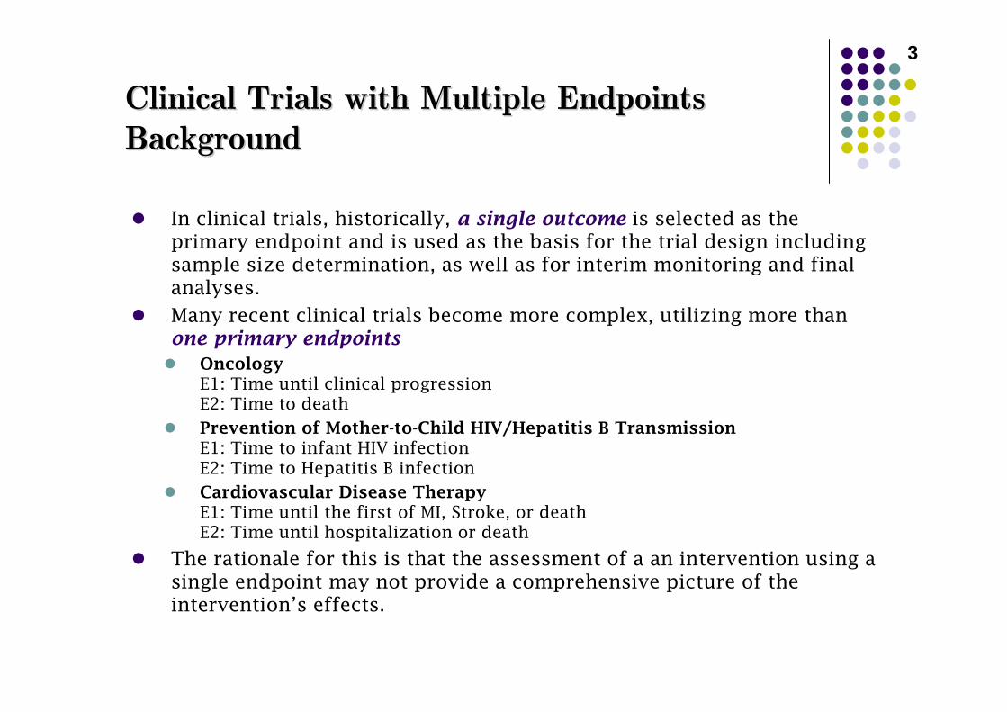
In clinical trials, historically, a single outcome is selected as the primary endpoint and is used as the basis for the trial design including sample size determination, as well as for interim monitoring and final analyses.
Many recent clinical trials become more complex, utilizing more than one primary endpoints
Oncology E1: Time until clinical progressionE2: Time to death
Prevention of Mother-to-Child HIV/Hepatitis B TransmissionE1: Time to infant HIV infectionE2: Time to Hepatitis B infection
Cardiovascular Disease TherapyE1: Time until the first of MI, Stroke, or deathE2: Time until hospitalization or death
The rationale for this is that the assessment of a an intervention using a single endpoint may not provide a comprehensive picture of the intervention’s effects.
Clinical Trials with Multiple EndpointsClinical Trials with Multiple EndpointsBackgroundBackground
4
Strategies for Multiple EndpointsStrategies for Multiple EndpointsBackgroundBackground
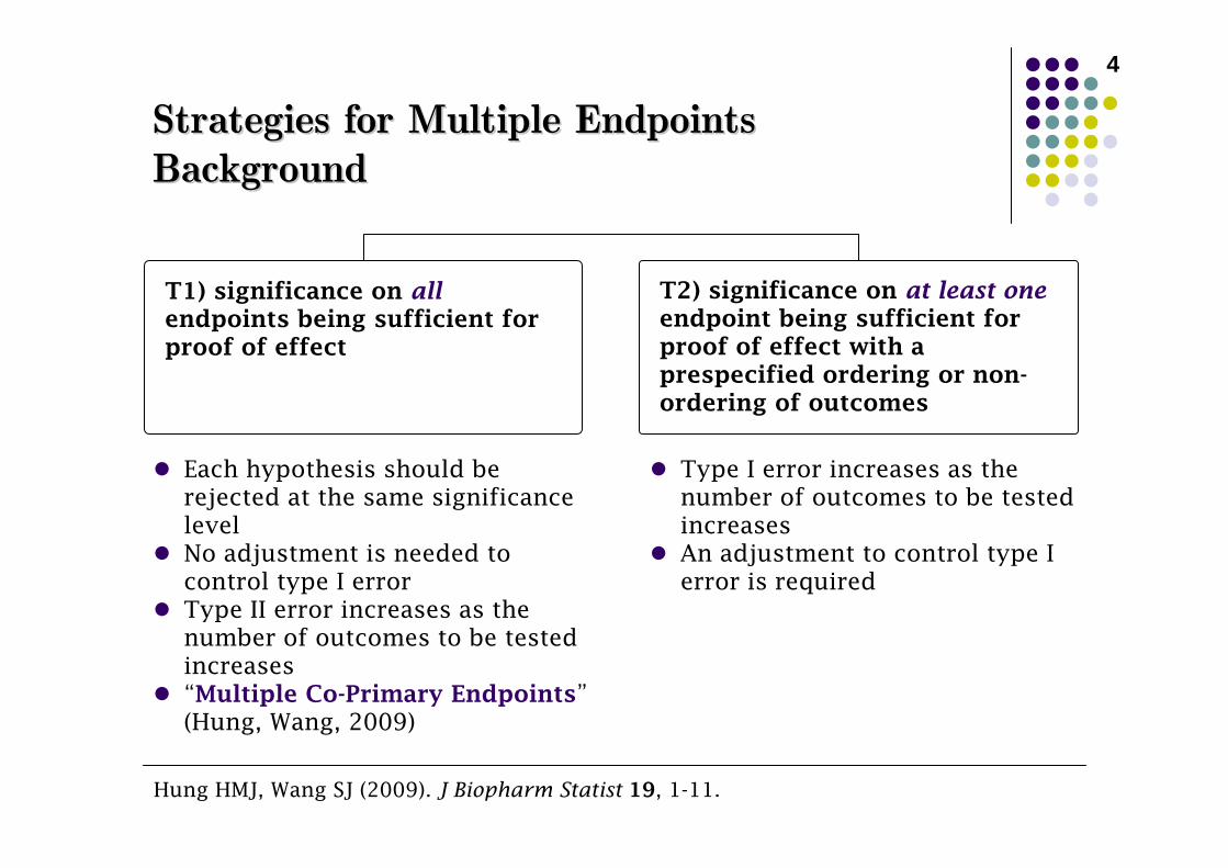
Each hypothesis should be rejected at the same significance level No adjustment is needed to control type I error Type II error increases as the number of outcomes to be tested increases“Multiple Co-Primary Endpoints”(Hung, Wang, 2009)
T1) significance on allendpoints being sufficient for proof of effect
Type I error increases as the number of outcomes to be tested increasesAn adjustment to control type I error is required
Hung HMJ, Wang SJ (2009). J Biopharm Statist 19, 1-11.
T2) significance on at least oneendpoint being sufficient for proof of effect with a prespecified ordering or non-ordering of outcomes

5
How large a sample should be for T1 and T2?
Is there any considerable overestimation or underestimation in the sample size when the correlation is ignored?
Is there any considerable reduction or increase in the sample size when the correlation is taken account into the sample size calculation ?
Arising Natural QuestionsArising Natural QuestionsBackgroundBackground

6
Our Research FocusOur Research FocusObjectivesObjectives
To discuss the power and sample size determination for superiority comparative clinical trials with two possibly correlated time-to-events endpoints to be evaluated as primary variables for the design and analysis, with paying more attention to T1
To consider a simpler approach that assumes that the time-to-event outcomes are exponentially distributed
Sugimoto et al (2011) discuss an approach to sizing clinical trials with two correlated time-to-event outcomes based on the log-rank statistics.
Implementing the method requires technical knowledge, sophisticated programming skill, and expensive computations
We will focus on hazard ratio : results of difference in hazard rates are very similar as seen in those of hazard ratios
Sugimoto T, Hamasaki T, Sozu T (2011). In Abstract of the 7th International Conference on Multiple Comparison Procedure, 121, Washington DC, USA, August 29-September 1, 2011.
7
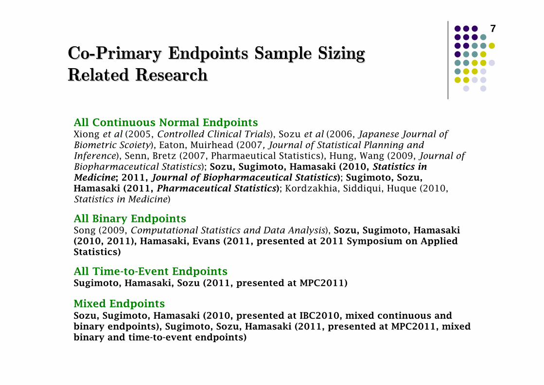
All Continuous Normal EndpointsXiong et al (2005, Controlled Clinical Trials), Sozu et al (2006, Japanese Journal of Biometric Scoiety), Eaton, Muirhead (2007, Journal of Statistical Planning and Inference), Senn, Bretz (2007, Pharmaeutical Statistics), Hung, Wang (2009, Journal of Biopharmaceutical Statistics); Sozu, Sugimoto, Hamasaki (2010, Statistics in Medicine; 2011, Journal of Biopharmaceutical Statistics); Sugimoto, Sozu, Hamasaki (2011, Pharmaceutical Statistics); Kordzakhia, Siddiqui, Huque (2010, Statistics in Medicine)
All Binary EndpointsSong (2009, Computational Statistics and Data Analysis), Sozu, Sugimoto, Hamasaki (2010, 2011), Hamasaki, Evans (2011, presented at 2011 Symposium on Applied Statistics)
All Time-to-Event EndpointsSugimoto, Hamasaki, Sozu (2011, presented at MPC2011)
Mixed EndpointsSozu, Sugimoto, Hamasaki (2010, presented at IBC2010, mixed continuous and binary endpoints), Sugimoto, Sozu, Hamasaki (2011, presented at MPC2011, mixed binary and time-to-event endpoints)
CoCo--Primary Endpoints Sample SizingPrimary Endpoints Sample SizingRelated ResearchRelated Research
8
OutlineOutline
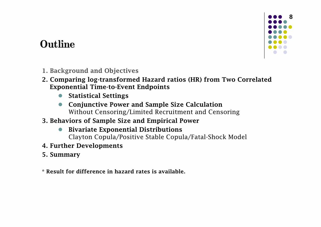
1. Background and Objectives
2. Comparing log-transformed Hazard ratios (HR) from Two Correlated Exponential Time-to-Event Endpoints
Statistical Settings
Conjunctive Power and Sample Size CalculationWithout Censoring/Limited Recruitment and Censoring
3. Behaviors of Sample Size and Empirical Power
Bivariate Exponential DistributionsClayton Copula/Positive Stable Copula/Fatal-Shock Model
4. Further Developments
5. Summary
* Result for difference in hazard rates is available.
2. Required Sample Size to Compare 2. Required Sample Size to Compare Hazard Ratio from Two Correlated Hazard Ratio from Two Correlated Exponential TimeExponential Time--toto--Event EndpointsEvent Endpoints
Statistical Setting
Conjunctive Power and Sample Size Calculation
10
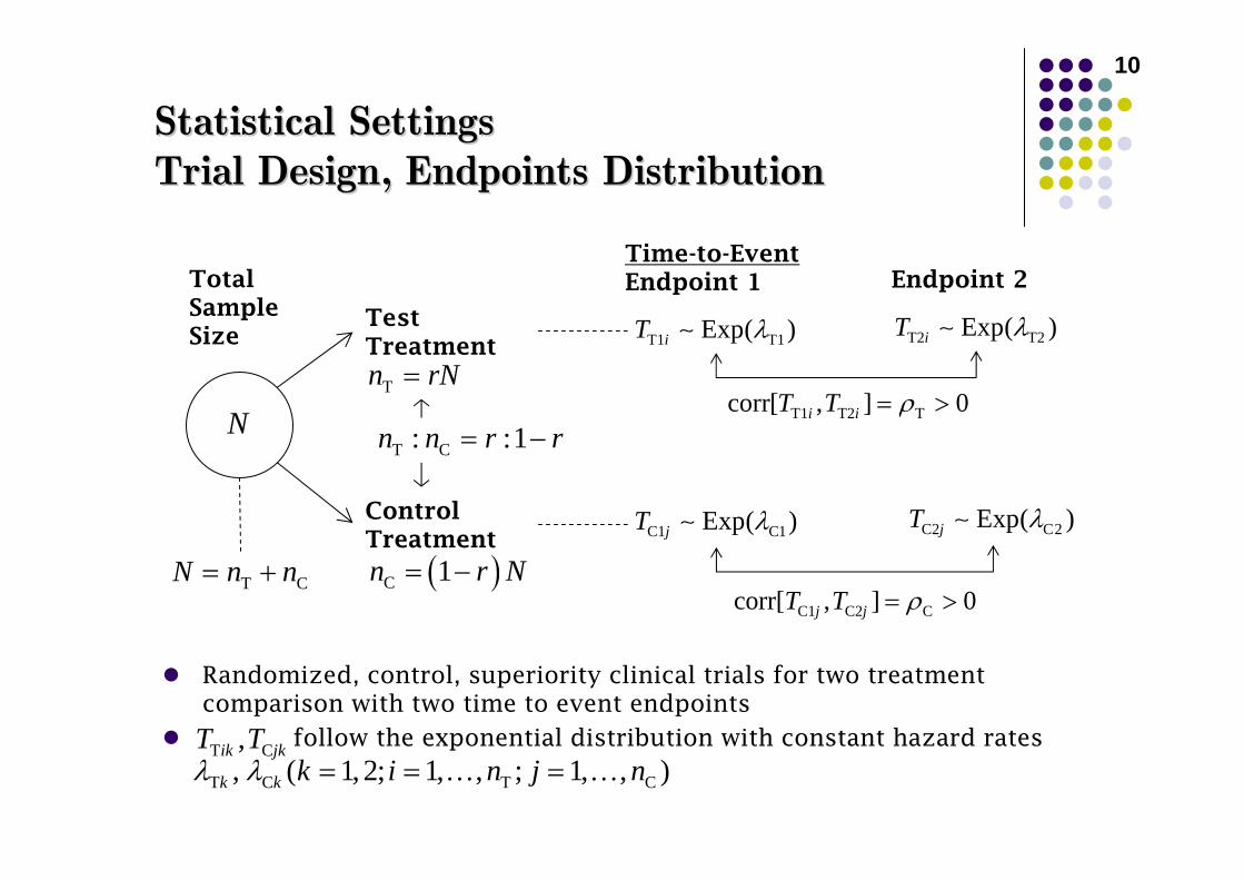
Randomized, control, superiority clinical trials for two treatment comparison with two time to event endpoints
follow the exponential distribution with constant hazard rates
Statistical SettingsStatistical SettingsTrial Design, Endpoints DistributionTrial Design, Endpoints Distribution
Test Treatment
ControlTreatment
Tn rN=
( )C 1n r N= −
N
T CN n n= +
Time-to-EventEndpoint 1 Endpoint 2 Total
Sample Size T1 T1Exp( )iT λ∼ T2 T2Exp( )iT λ∼
C1 C1Exp( )jT λ∼ C2 C2Exp( )jT λ∼
T1 T2 Tcorr[ , ] 0i iT T ρ= >
C1 C2 Ccorr[ , ] 0j jT T ρ= >
T C: :1n n r r= −
T C,ik jkT TT C T C, ( 1, 2; 1, , ; 1, , )k k k i n j nλ λ = = =… …
11
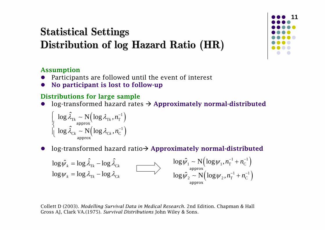
Statistical SettingsStatistical SettingsDistribution of log Hazard Ratio (HR)Distribution of log Hazard Ratio (HR)
AssumptionParticipants are followed until the event of interestNo participant is lost to follow-up
Distributions for large samplelog-transformed hazard rates Approximately normal-distributed
log-transformed hazard ratio Approximately normal-distributed
( )( )
1T T T
1C C C
ˆlog N log ,
ˆlog N log ,
k k
k k
n
n
λ λ
λ λ
−
−
⎧⎪⎨⎪⎩
∼
∼
T C
T C
ˆ ˆˆlog log loglog log log
k k k
k k k
ψ λ λψ λ λ
= −
= −
approx
approx
( )( )
1 11 1 T C
1 12 2 T C
ˆlog N log ,
ˆlog N log ,
n n
n n
ψ ψ
ψ ψ
− −
− −
+
+
∼
∼approx
approx
Collett D (2003). Modelling Survival Data in Medical Research. 2nd Edition. Chapman & HallGross AJ, Clark VA.(1975). Survival Distributions John Wiley & Sons.
12
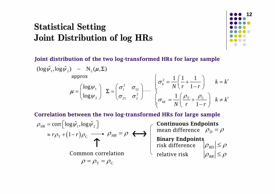
Statistical SettingStatistical SettingJoint Distribution of log Joint Distribution of log HRsHRs
1 2 2ˆ ˆ(log , log ) N ( , )ψ ψ ∼ μ Σ
21 1 12
22 21 2
loglog
ψ σ σψ σ σ
⎛ ⎞⎛ ⎞= = ⎜ ⎟⎜ ⎟⎝ ⎠ ⎝ ⎠
μ Σ
2
CT
1 1 11
11
k
kk
k kN r r
k kN r r
σ
ρρσ ′
⎧ ⎛ ⎞ ′= + =⎪ ⎜ ⎟−⎝ ⎠⎪⎨
⎛ ⎞⎪ ′= + ≠⎜ ⎟⎪ −⎝ ⎠⎩
approx
( )1 2
T C
ˆ ˆcorr log , log
1HR
r r
ρ ψ ψ
ρ ρ
= ⎡ ⎤⎣ ⎦≈ + −
T Cρ ρ ρ= =
HRρ ρ=Continuous Endpointsmean difference
Binary Endpointsrisk difference
relative risk
Dρ ρ=
RRρ ρ≤RDρ ρ≤
Correlation between the two log-transformed HRs for large sample
Joint distribution of the two log-transformed HRs for large sample
Common correlation
13
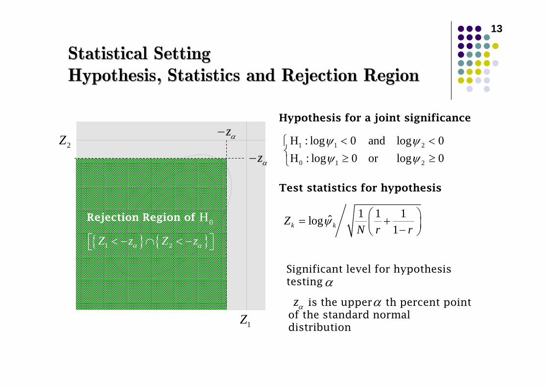
Statistical Setting Statistical Setting Hypothesis, Statistics and Rejection RegionHypothesis, Statistics and Rejection Region
1 1 2
0 1 2
H : log 0 and log 0H : log 0 or log 0
ψ ψψ ψ
< <⎧⎨ ≥ ≥⎩
1 1 1ˆlog1k kZ
N r rψ ⎛ ⎞= +⎜ ⎟−⎝ ⎠
Hypothesis for a joint significance
Test statistics for hypothesis
is the upper th percent point of the standard normal distribution
zα α
zα−
zα−
1Z
2Z
{ } { }1 2Z z Z zα α⎡ ⎤< − ∩ < −⎣ ⎦
Rejection Region of 0H
Significant level for hypothesis testing α
14
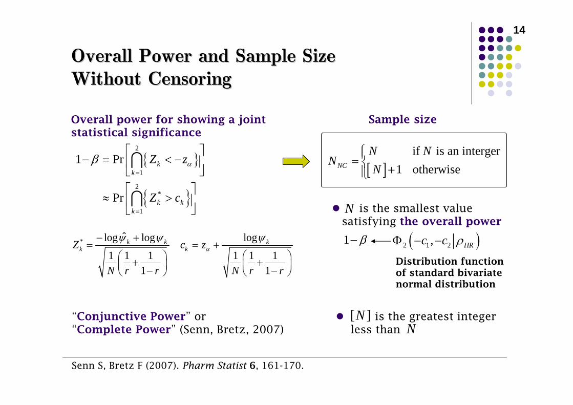
is the greatest integer less than
is the smallest value satisfying the overall power
Overall power for showing a joint statistical significance
Overall Power and Sample SizeOverall Power and Sample SizeWithout CensoringWithout Censoring
{ }
{ }
2
1
2*
1
1 Pr
Pr
kk
k kk
Z z
Z c
αβ=
=
⎡ ⎤− = < −⎢ ⎥
⎣ ⎦⎡ ⎤
≈ >⎢ ⎥⎣ ⎦
∩
∩
* ˆlog log log
1 1 1 1 1 11 1
k k kk kZ c z
N r r N r r
αψ ψ ψ− +
= = +⎛ ⎞ ⎛ ⎞+ +⎜ ⎟ ⎜ ⎟− −⎝ ⎠ ⎝ ⎠
1 β−
Distribution function of standard bivariate normal distribution
Senn S, Bretz F (2007). Pharm Statist 6, 161-170.
Sample size
[ ]if is an interger
1 otherwiseNC
N NN
N⎧⎪= ⎨ +⎪⎩
N
[ ]NN
( )2 1 2, HRc c ρΦ − −
“Conjunctive Power” or “Complete Power” (Senn, Bretz, 2007)
15
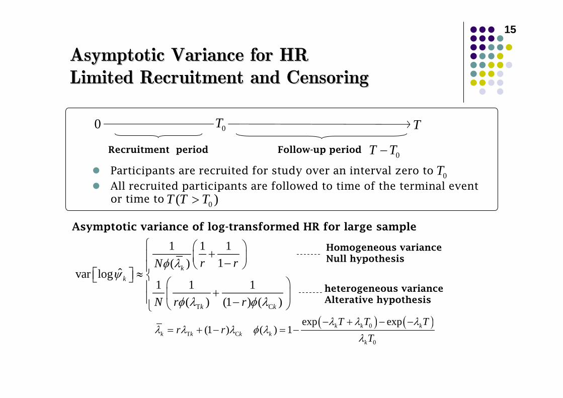
Participants are recruited for study over an interval zero to
All recruited participants are followed to time of the terminal event or time to
Asymptotic Variance for HRAsymptotic Variance for HRLimited Recruitment and CensoringLimited Recruitment and Censoring
0( )T T T>
T C
1 1 11( )
ˆvar log1 1 1
( ) (1 ) ( )
kk
k k
r rN
N r r
φ λψ
φ λ φ λ
⎧ ⎛ ⎞+⎪ ⎜ ⎟−⎝ ⎠⎪≈⎡ ⎤ ⎨⎣ ⎦ ⎛ ⎞⎪ +⎜ ⎟⎪ −⎝ ⎠⎩( ) ( )0
T C0
exp exp(1 ) ( ) 1 k k k
k k k kk
T T Tr r
Tλ λ λ
λ λ λ φ λλ
− + − −= + − = −
0T0 T
Recruitment period Follow-up period 0T T−
0T
Asymptotic variance of log-transformed HR for large sample
Homogeneous varianceNull hypothesis
heterogeneous varianceAlterative hypothesis
16
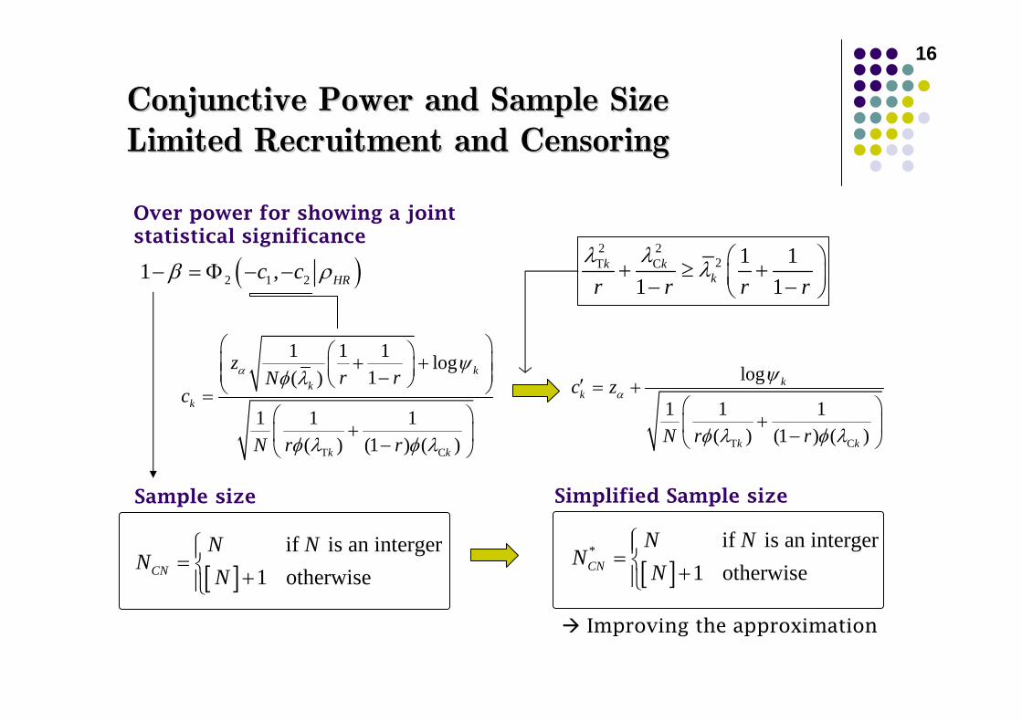
Over power for showing a joint statistical significance
Conjunctive Power and Sample SizeConjunctive Power and Sample SizeLimited Recruitment and CensoringLimited Recruitment and Censoring
T C
1 1 1 log1( )
1 1 1( ) (1 ) ( )
kk
k
k k
zr rN
c
N r r
α ψφ λ
φ λ φ λ
⎛ ⎞⎛ ⎞+ +⎜ ⎟⎜ ⎟⎜ ⎟−⎝ ⎠⎝ ⎠=⎛ ⎞
+⎜ ⎟−⎝ ⎠
( )2 1 21 , HRc cβ ρ− = Φ − −
[ ]if is an interger
1 otherwiseCN
N NN
N⎧⎪= ⎨ +⎪⎩
Sample size
2 22T C 1 1
1 1k k
kr r r rλ λ
λ ⎛ ⎞+ ≥ +⎜ ⎟− −⎝ ⎠
[ ]* if is an interger
1 otherwiseCN
N NN
N⎧⎪= ⎨ +⎪⎩
Simplified Sample size
Improving the approximation
T C
log
1 1 1( ) (1 ) ( )
kk
k k
c z
N r r
αψ
φ λ φ λ
′ = +⎛ ⎞
+⎜ ⎟−⎝ ⎠
17
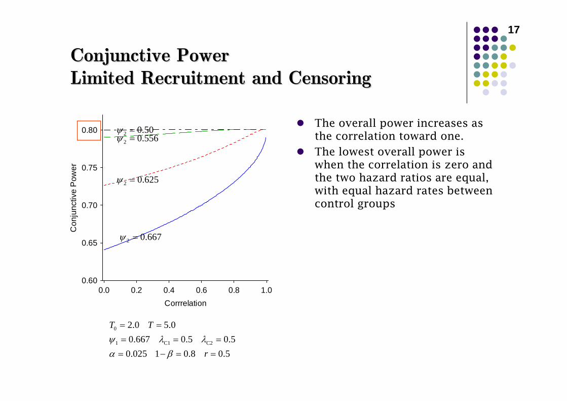
Conjunctive PowerConjunctive PowerLimited Recruitment and CensoringLimited Recruitment and Censoring
The overall power increases as the correlation toward one.
The lowest overall power is when the correlation is zero and the two hazard ratios are equal, with equal hazard rates between control groups
0.0 0.2 0.4 0.6 0.8 1.0Corrrelation
0.60
0.65
0.70
0.75
0.80
Con
junc
tive
Pow
er
0
1 C1 C2
2.0 5.00.667 0.5 0.5
0.025 1 0.8 0.5
T T
rψ λ λα β
= == = =
= − = =
2 0.667ψ =
2 0.625ψ =
2 0.556ψ =2 0.50ψ =
3. Behaviors of Sample Size and 3. Behaviors of Sample Size and Empirical PowerEmpirical Power
Bivariate Exponential Distributions
Sample Size Behavior
Empirical Power for Log-Rank Test
19
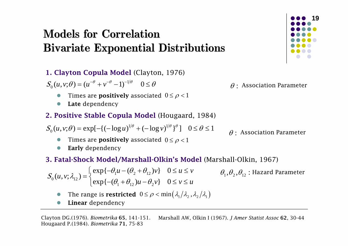
1. Clayton Copula Model (Clayton, 1976)
Times are positively associated
Late dependency
2. Positive Stable Copula Model (Hougaard, 1984)
Times are positively associated
Early dependency
3. Fatal-Shock Model/Marshall-Olkin’s Model (Marshall-Olkin, 1967)
The range is restricted
Linear dependency
Models for CorrelationModels for CorrelationBivariate Exponential DistributionsBivariate Exponential Distributions
( )1 2 2 10 min ,ρ λ λ λ λ≤ <
10 ( , ; ) ( 1) 0u v u vθ θ θθ θ− − −= + − ≤S
0 1ρ≤ <
1 10 ( , ; ) exp[ {( log ) ( log ) } ] 0 1u v u vθ θ θθ θ= − − + − ≤ ≤S
0 1ρ≤ <
:θ Association Parameter
:θ Association Parameter
1 2 120 12
1 12 2
exp{ ( ) } 0( , ; )
exp{ ( ) } 0u v u v
u vu v v u
θ θ θλ
θ θ θ− − + ≤ ≤⎧
= ⎨ − + − ≤ ≤⎩S 1 2 12, , :θ θ θ Hazard Parameter
Clayton DG.(1976). Biometrika 65, 141-151. Hougaard P.(1984). Biometrika 71, 75-83
Marshall AW, Olkin I (1967). J Amer Statist Assoc 62, 30-44
20
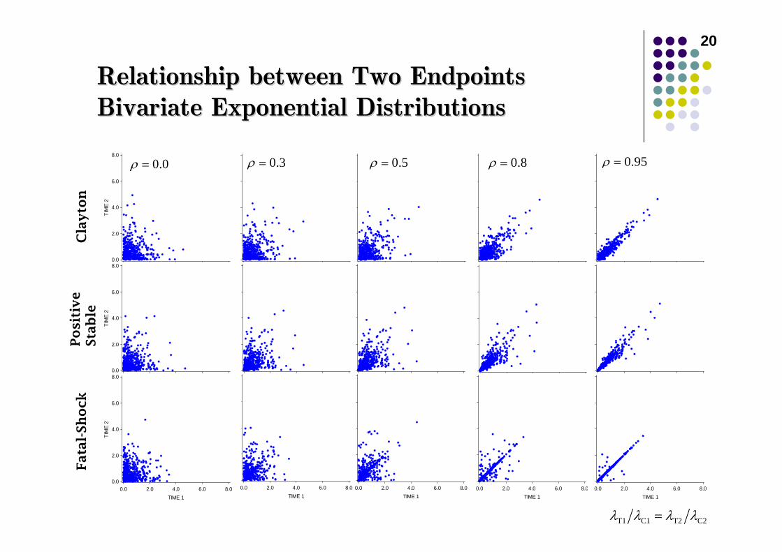
Relationship between Two Endpoints Relationship between Two Endpoints Bivariate Exponential DistributionsBivariate Exponential Distributions
0.0
2.0
4.0
6.0
8.0
TIM
E 2
0 0 2 0 4 0 6 0 8 00.0
2.0
4.0
6.0
8.0
TIM
E 2
0.0 2.0 4.0 6.0 8.0TIME 1
0.0
2.0
4.0
6.0
8.0
TIM
E 2
0.0 2.0 4.0 6.0 8.0TIME 1
0.0 2.0 4.0 6.0 8.0TIME 1
0.0 2.0 4.0 6.0 8.0TIME 1
Fata
l-Sh
ock
Cla
yto
nPosi
tive
Sta
ble
0.0ρ = 0.3ρ = 0.5ρ = 0.8ρ = 0.95ρ =
0.0 2.0 4.0 6.0 8.0TIME 1
T1 C1 T2 C2λ λ λ λ=
21
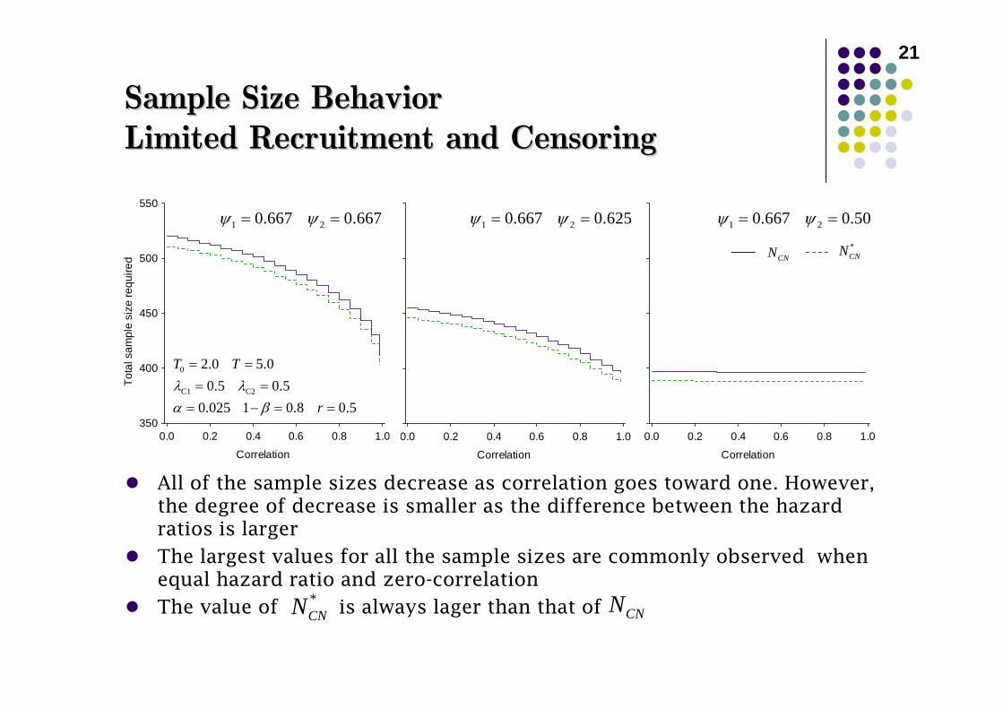
Sample Size BehaviorSample Size BehaviorLimited Recruitment and CensoringLimited Recruitment and Censoring
All of the sample sizes decrease as correlation goes toward one. However, the degree of decrease is smaller as the difference between the hazard ratios is larger
The largest values for all the sample sizes are commonly observed when equal hazard ratio and zero-correlation
The value of is always lager than that of
Correlation
0.0 0.2 0.4 0.6 0.8 1.0Correlation
Tota
l sam
ple
size
requ
ired
0.0 0.2 0.4 0.6 0.8 1.0350
400
450
500
550
Correlation
0.0 0.2 0.4 0.6 0.8 1.0
0
C1 C2
2.0 5.00.5 0.5
0.025 1 0.8 0.5
T T
rλ λα β
= == =
= − = =
*CNN CNN
1 20.667 0.667ψ ψ= = 1 20.667 0.625ψ ψ= = 1 20.667 0.50ψ ψ= =
CNN *CNN
22
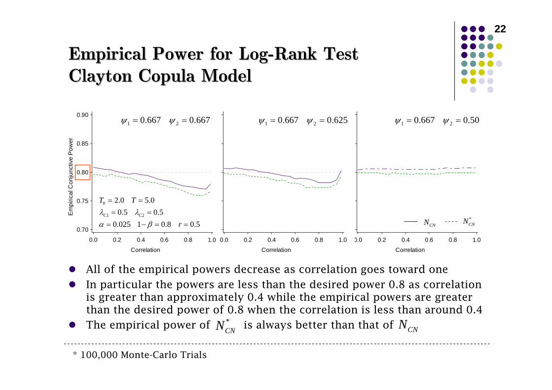
Empirical Power for LogEmpirical Power for Log--Rank TestRank TestClayton Copula ModelClayton Copula Model
All of the empirical powers decrease as correlation goes toward one
In particular the powers are less than the desired power 0.8 as correlation is greater than approximately 0.4 while the empirical powers are greater than the desired power of 0.8 when the correlation is less than around 0.4
The empirical power of is always better than that of
Correlation
Em
piric
al C
onju
nctiv
e P
ower
0.0 0.2 0.4 0.6 0.8 1.0
0.70
0.75
0.80
0.85
0.90
Correlation
0.0 0.2 0.4 0.6 0.8 1.0
Correlation
0.0 0.2 0.4 0.6 0.8 1.0
1 20.667 0.667ψ ψ= =
0
C1 C2
2.0 5.00.5 0.5
0.025 1 0.8 0.5
T T
rλ λα β
= == =
= − = =
*CNN CNN
1 20.667 0.625ψ ψ= = 1 20.667 0.50ψ ψ= =
CNN *CNN
* 100,000 Monte-Carlo Trials
23
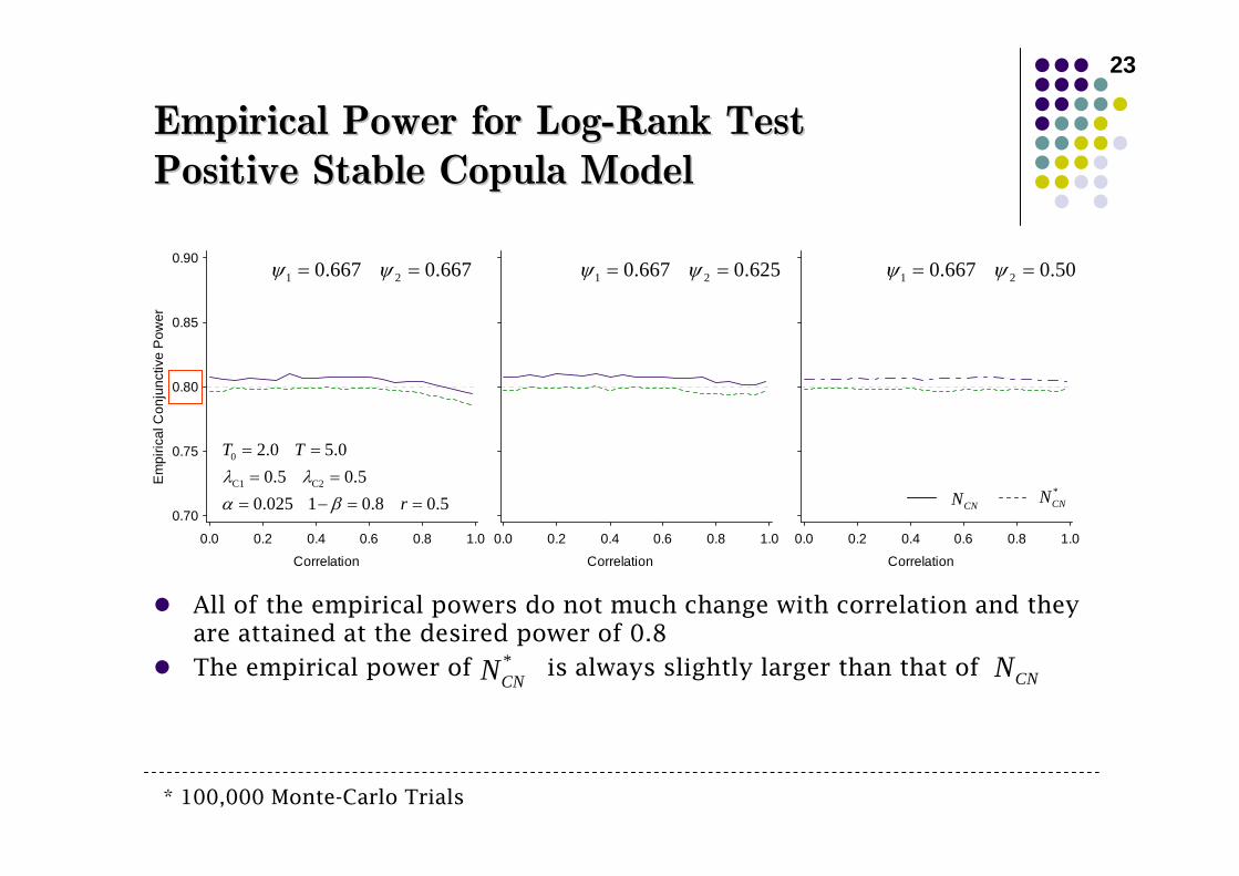
Empirical Power for LogEmpirical Power for Log--Rank TestRank TestPositive Stable Copula ModelPositive Stable Copula Model
Correlation
Em
piric
al C
onju
nctiv
e P
ower
0.0 0.2 0.4 0.6 0.8 1.0
0.70
0.75
0.80
0.85
0.90
Correlation
0.0 0.2 0.4 0.6 0.8 1.0
Correlation
0.0 0.2 0.4 0.6 0.8 1.0
0
C1 C2
2.0 5.00.5 0.5
0.025 1 0.8 0.5
T T
rλ λα β
= == =
= − = =
All of the empirical powers do not much change with correlation and they are attained at the desired power of 0.8
The empirical power of is always slightly larger than that of *CNN CNN
1 20.667 0.667ψ ψ= = 1 20.667 0.625ψ ψ= = 1 20.667 0.50ψ ψ= =
CNN *CNN
* 100,000 Monte-Carlo Trials
24
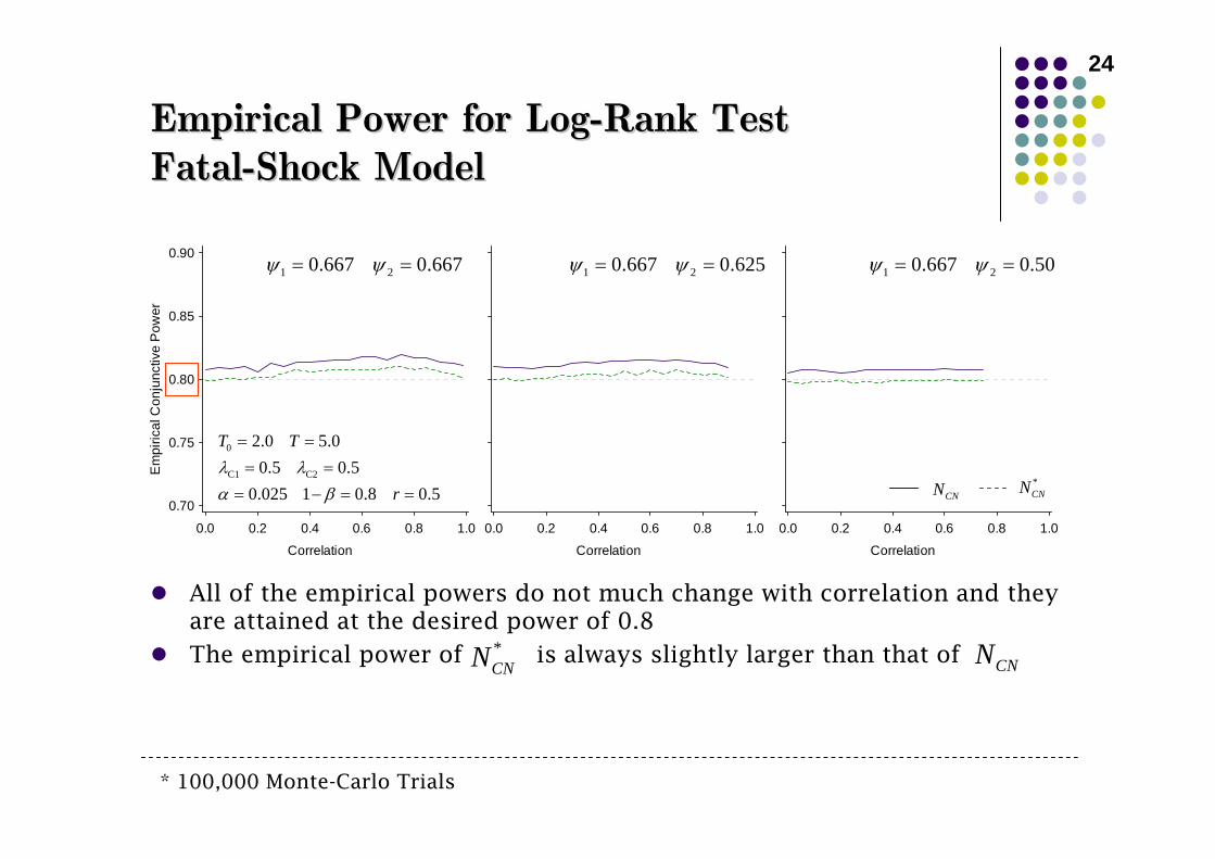
Empirical Power for LogEmpirical Power for Log--Rank TestRank TestFatalFatal--Shock ModelShock Model
Correlation
Em
piric
al C
onju
nctiv
e P
ower
0.0 0.2 0.4 0.6 0.8 1.0
0.70
0.75
0.80
0.85
0.90
Correlation
0.0 0.2 0.4 0.6 0.8 1.0
Correlation
0.0 0.2 0.4 0.6 0.8 1.0
0
C1 C2
2.0 5.00.5 0.5
0.025 1 0.8 0.5
T T
rλ λα β
= == =
= − = =
All of the empirical powers do not much change with correlation and they are attained at the desired power of 0.8
The empirical power of is always slightly larger than that of *CNN CNN
1 20.667 0.667ψ ψ= = 1 20.667 0.625ψ ψ= = 1 20.667 0.50ψ ψ= =
CNN *CNN
* 100,000 Monte-Carlo Trials
4. Further Developments4. Further Developments
At Least One Statistical Significance
Non-Inferiority Hypothesis
Mixed Binary and Time-to-Event Endpoints

26
At Least One Statistical SignificanceAt Least One Statistical SignificancePower for Bonferroni Adjustment Power for Bonferroni Adjustment
0.0 0.2 0.4 0.6 0.8 1.0Corrrelation
0.0
0.1
0.2
0.3
0.4
0.5
0.6
0.7
0.8
0.9
1.0
Dis
junc
tive
Pow
er
2 0.667ψ =
2 0.625ψ =
2 0.556ψ =
2 0.50ψ =
0.0 0.2 0.4 0.6 0.8 1.0Correlation
1.0
1.1
1.2
1.3
1.4
1.5
1.6
1.7
Rat
io o
f Tot
al S
ampl
e S
ize
Req
uire
d2 0.667ψ =
2 0.625ψ =
2 0.556ψ =
2 0.50ψ =0
1 C1 C2
2.0 5.00.667 0.5 0.5
0.025 1 0.8 0.5
T T
rψ λ λα β
= == = == − = =
Overall power for showing statistical significance for at least oneendpoint with Bonferroni adjustment
{ }2
21
1 1 Pr kk
Z zαβ=
⎡ ⎤− = − > −⎢ ⎥
⎣ ⎦∩ “Disjunctive power” or “Minimal power”
(Senn, Bretz, 2007).
27
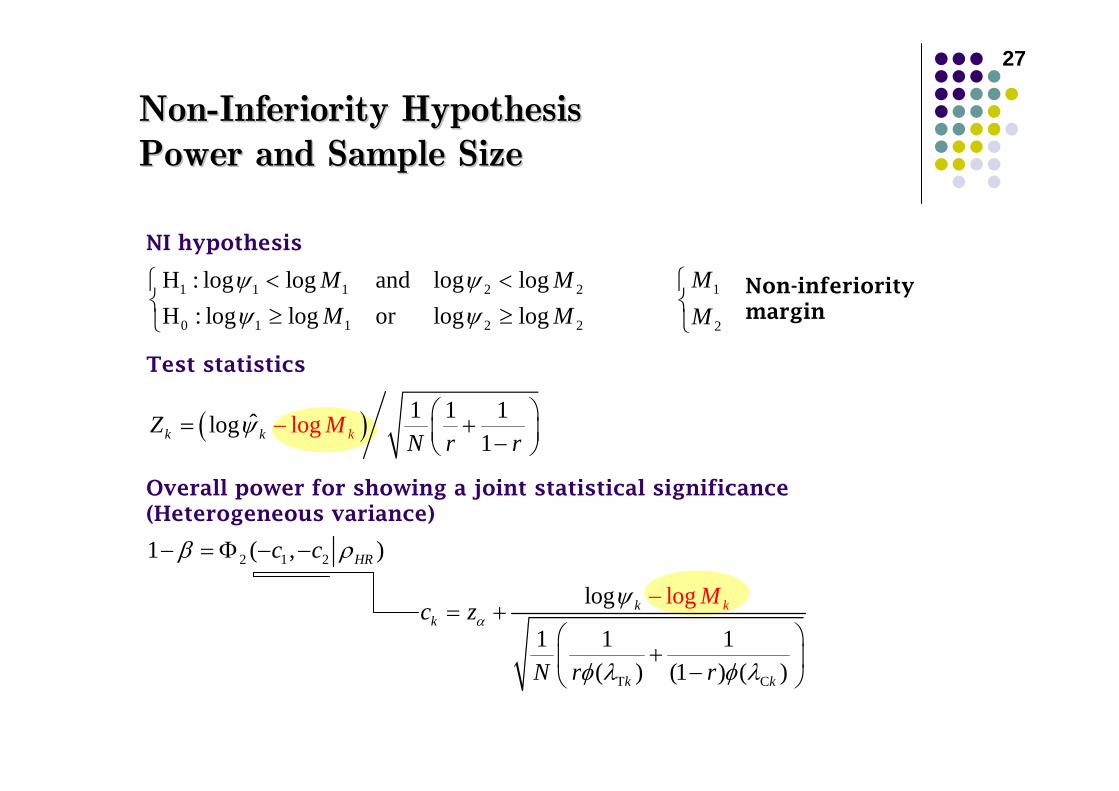
NI hypothesis
Test statistics
Overall power for showing a joint statistical significance (Heterogeneous variance)
NonNon--Inferiority HypothesisInferiority HypothesisPower and Sample SizePower and Sample Size
1 1 1 2 2
0 1 1 2 2
H : log log and log logH : log log or log log
M MM M
ψ ψψ ψ
< <⎧⎨ ≥ ≥⎩
( ) 1 1 1oˆog gl1
lk k kZ MN r r
ψ ⎛ ⎞= +⎜ ⎟−⎝ ⎠−
1
2
MM⎧⎨⎩
Non-inferiority margin
2 1 21 ( , )HRc cβ ρ− = Φ − −
T C
log
1 1 1( ) (1 ) (
log
)
kkk
k k
c zM
N r r
αψ
φ λ φ λ
= +⎛ ⎞
+⎜ ⎟−⎝ ⎠
−
28
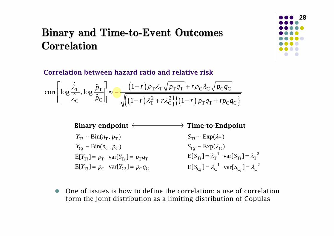
Correlation between hazard ratio and relative risk
Binary and TimeBinary and Time--toto--Event Outcomes Event Outcomes CorrelationCorrelation
( )( ){ } ( ){ }
T T T T C C C CT T
2 2CC T C T T C C
ˆ 1ˆcorr log , logˆ ˆ 1 1
r p q r p qpp r r r p q rp q
ρ λ ρ λλλ λ λ
⎡ ⎤ − +≈⎢ ⎥
⎢ ⎥⎣ ⎦ − + − +−
T T T T T
T C C C C
E[ ] var[ ]E[ ] var[ ]
i i
j j
Y p Y p qY p Y p q
= =
= =
1 2T T T T
1 2C C C C
E[ ] var[ ]
E[ ] var[ ]i i
j j
S S
S S
λ λ
λ λ
− −
− −
= =
= =
T T T
C C C
Bin( , )Bin( , )
i
j
Y n pY n p∼∼
T T
C C
Exp( )Exp( )
i
j
SS
λλ
∼∼
Binary endpoint Time-to-Endpoint
One of issues is how to define the correlation: a use of correlation form the joint distribution as a limiting distribution of Copulas
5. Summary5. Summary
30
SummarySummary
We described the power and sample size determination for comparative clinical trials with two correlated time-to-event endpoints to be evaluated as primary variables.
A simpler approach that assumes that the time-to-event endpoints are exponentially distributed.
Displaying significance on both endpoints for proof of an acceptable efficacy profile
The method may work when the dependency structure is early or linear one. While a careful use of the method is recommended when the late high dependency is observed.
Our research is restricted to “two treatment comparison and twotime-to-event endpoints”
The result from two endpoints gains the insight into more than two endpoints
The extension of the result to more than two hazard ratios is not difficult although other issues will arise.