Embed Size (px)
Citation preview
Sample Size calculations for Stepped Wedge Trials
Gianluca Baio
University College LondonDepartment of Statistical Science
(Joint work with Rumana Omar, Andrew Copas, Emma Beard, James Hargreaves and Gareth Ambler)
Stepped Wedge Trials SymposiumLondon School of Hygiene & Tropical Medicine
London, 22 September 2015
Gianluca Baio ( UCL) Sample size calculations for SWTs LSHTM Symposium, 22 Sep 2015 1 / 10

Objectives of the project/paper
Work supported by a NIHR Research Methods Opportunity Funding SchemeGrant (RMOFS-2013-03-02)
• Critically investigate the conditions under which applying a stepped wedgedesign can result in potential gains in terms of
– Efficiency– Statistical power– Financial/ethical implications
• Produce a toolbox to perform power calculations
– Simulation-based approach– Extension to more general models
• Have lots of fun working in the “Special Issue Crew”!
Gianluca Baio ( UCL) Sample size calculations for SWTs LSHTM Symposium, 22 Sep 2015 2 / 10
Modelling & sample size calculations
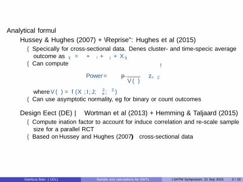
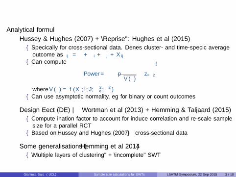
Analytical formulæ
• Hussey & Hughes (2007) + “Reprise”: Hughes et al (2015)
– Specifically for cross-sectional data. Defines cluster- and time-specific averageoutcome as µij = µ+ αi + βj +Xijθ
– Can compute
Power = Φ
(θ√V (θ)
− zα/2
)where V (θ) = f(X, I, J, σ2
e , σ2α)
– Can use asymptotic normality, eg for binary or count outcomes
• Design Effect (DE) — Wortman et al (2013) + Hemming & Taljaard (2015)
– Compute inflation factor to account for induce correlation and re-scale samplesize for a parallel RCT
– Based on Hussey and Hughes (2007) ⇒ cross-sectional data
• Some generalisations (Hemming et al 2014)
– “Multiple layers of clustering” + “incomplete” SWT
Gianluca Baio ( UCL) Sample size calculations for SWTs LSHTM Symposium, 22 Sep 2015 3 / 10

Modelling & sample size calculations
Analytical formulæ
• Hussey & Hughes (2007) + “Reprise”: Hughes et al (2015)
– Specifically for cross-sectional data. Defines cluster- and time-specific averageoutcome as µij = µ+ αi + βj +Xijθ
– Can compute
Power = Φ
(θ√V (θ)
− zα/2
)where V (θ) = f(X, I, J, σ2
e , σ2α)
– Can use asymptotic normality, eg for binary or count outcomes
• Design Effect (DE) — Wortman et al (2013) + Hemming & Taljaard (2015)
– Compute inflation factor to account for induce correlation and re-scale samplesize for a parallel RCT
– Based on Hussey and Hughes (2007) ⇒ cross-sectional data
• Some generalisations (Hemming et al 2014)
– “Multiple layers of clustering” + “incomplete” SWT
Gianluca Baio ( UCL) Sample size calculations for SWTs LSHTM Symposium, 22 Sep 2015 3 / 10
Modelling & sample size calculations
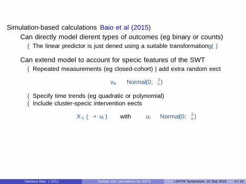
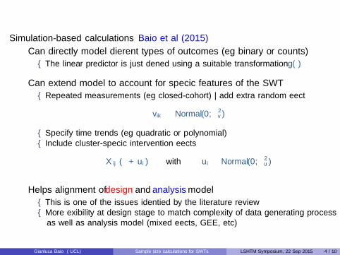
Simulation-based calculations Baio et al (2015)
• Can directly model different types of outcomes (eg binary or counts)
– The linear predictor is just defined using a suitable transformation g(·)
• Can extend model to account for specific features of the SWT
– Repeated measurements (eg closed-cohort) — add extra random effect
vik ∼ Normal(0, σ2v)
– Specify time trends (eg quadratic or polynomial)– Include cluster-specific intervention effects
Xij(θ + ui) with ui ∼ Normal(0, σ2u)
• Helps alignment of design and analysis model
– This is one of the issues identified by the literature review– More flexibility at design stage to match complexity of data generating process
as well as analysis model (mixed effects, GEE, etc)
Gianluca Baio ( UCL) Sample size calculations for SWTs LSHTM Symposium, 22 Sep 2015 4 / 10
Modelling & sample size calculations
Simulation-based calculations Baio et al (2015)
• Can directly model different types of outcomes (eg binary or counts)
– The linear predictor is just defined using a suitable transformation g(·)
• Can extend model to account for specific features of the SWT
– Repeated measurements (eg closed-cohort) — add extra random effect
vik ∼ Normal(0, σ2v)
– Specify time trends (eg quadratic or polynomial)– Include cluster-specific intervention effects
Xij(θ + ui) with ui ∼ Normal(0, σ2u)
• Helps alignment of design and analysis model
– This is one of the issues identified by the literature review– More flexibility at design stage to match complexity of data generating process
as well as analysis model (mixed effects, GEE, etc)
Gianluca Baio ( UCL) Sample size calculations for SWTs LSHTM Symposium, 22 Sep 2015 4 / 10
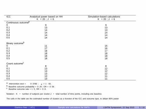
Simulation-based vs analytical calculations
ICC Analytical power based on HH Simulation-based calculationsK = 20, J = 6 K = 20, J = 6
Continuous outcomea
0 9 90.1 13 130.2 14 130.3 14 140.4 14 140.5 14 14
Binary outcomeb
0 11 150.1 17 160.2 18 170.3 18 180.4 18 180.5 18 18
Count outcomec
0 8 80.1 13 120.2 13 120.3 13 120.4 13 110.5 13 11
a Intervention effect = −0.3785; σe = 1.55.b Baseline outcome probability = 0.26; OR = 0.56.c Baseline outcome rate = 1.5; RR = 0.8.
Notation: K = number of subjects per cluster; J = total number of time points, including one baseline.
The cells in the table are the estimated number of clusters as a function of the ICC and outcome type, to obtain 80% power
Gianluca Baio ( UCL) Sample size calculations for SWTs LSHTM Symposium, 22 Sep 2015 5 / 10
Cross-sectional vs closed-cohort data
Effect size & ICC — Continuous outcome
Cross-sectional Closed-cohort
I = 25 clusters, each with K = 20 subjects; J = 6 time points (≡ measurements) including one baseline
Gianluca Baio ( UCL) Sample size calculations for SWTs LSHTM Symposium, 22 Sep 2015 6 / 10
Cross-sectional vs closed-cohort data
Number of steps — Binary outcome
Cross-sectional Closed-cohort
I = 24 clusters, each with K = 20 subjects; individual-level ICC= 0.0016 for closed-cohort
Gianluca Baio ( UCL) Sample size calculations for SWTs LSHTM Symposium, 22 Sep 2015 7 / 10
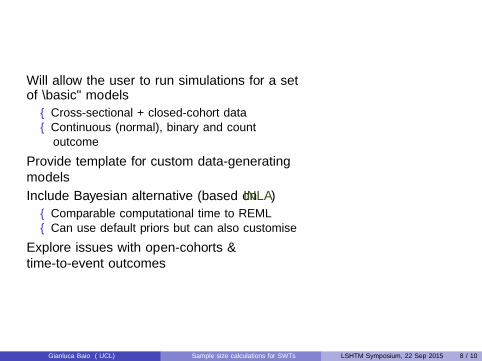
R package SWSamp
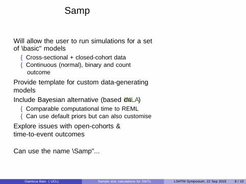
• Will allow the user to run simulations for a setof “basic” models
– Cross-sectional + closed-cohort data– Continuous (normal), binary and count
outcome
• Provide template for custom data-generatingmodels
• Include Bayesian alternative (based on INLA)
– Comparable computational time to REML– Can use default priors but can also customise
• Explore issues with open-cohorts &time-to-event outcomes
• Can use the name “Samp”...
Gianluca Baio ( UCL) Sample size calculations for SWTs LSHTM Symposium, 22 Sep 2015 8 / 10
R package SWSamp
• Will allow the user to run simulations for a setof “basic” models
– Cross-sectional + closed-cohort data– Continuous (normal), binary and count
outcome
• Provide template for custom data-generatingmodels
• Include Bayesian alternative (based on INLA)
– Comparable computational time to REML– Can use default priors but can also customise
• Explore issues with open-cohorts &time-to-event outcomes
• Can use the name “Samp”...
Gianluca Baio ( UCL) Sample size calculations for SWTs LSHTM Symposium, 22 Sep 2015 8 / 10
(Only a very few!) References
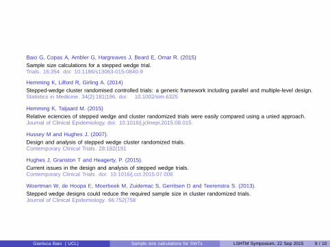
Baio G, Copas A, Ambler G, Hargreaves J, Beard E, Omar R. (2015)
Sample size calculations for a stepped wedge trial.Trials. 16:354. doi: 10.1186/s13063-015-0840-9
Hemming K, Lilford R, Girling A. (2014)
Stepped-wedge cluster randomised controlled trials: a generic framework including parallel and multiple-level design.Statistics in Medicine. 34(2):181—196. doi: 10.1002/sim.6325
Hemming K, Taljaard M. (2015)
Relative efficiencies of stepped wedge and cluster randomized trials were easily compared using a unified approach.Journal of Clinical Epidemiology. doi: 10.1016/j.jclinepi.2015.08.015.
Hussey M and Hughes J. (2007).
Design and analysis of stepped wedge cluster randomized trials.Contemporary Clinical Trials. 28:182–191
Hughes J, Granston T and Heagerty, P. (2015).
Current issues in the design and analysis of stepped wedge trials.Contemporary Clinical Trials. doi: 10.1016/j.cct.2015.07.006
Woertman W, de Hoopa E, Moerbeek M, Zuidemac S, Gerritsen D and Teerenstra S. (2013).
Stepped wedge designs could reduce the required sample size in cluster randomized trials.Journal of Clinical Epidemiology . 66:752–758
Gianluca Baio ( UCL) Sample size calculations for SWTs LSHTM Symposium, 22 Sep 2015 9 / 10
Thank you!
Gianluca Baio ( UCL) Sample size calculations for SWTs LSHTM Symposium, 22 Sep 2015 10 / 10