Embed Size (px)
Citation preview

SAMPLE REPORT
Iowa State University Industrial Assessment Center
(A U.S. Department of Energy Sponsored Program)
INDUSTRIAL ASSESSMENT REPORT
No. 666
AUDIT DATE: March 1, 2005
LOCATION: Ames, IA – Story county
PRINCIPAL PRODUCTS: Industrial Equipment
S.I.C. CODE: 3266
N.A.I.C.S. CODE: 335894
REPORT DATE: April 1, 2005
Team Leader: Dr. Greg Maxwell
Pablo Rivera, Graduate Engineer1 Eric Kamm, Student Engineer Alex Rodrigues, Graduate Engineer2 Trevor Gilbertson, Student Engineer 1 Lead Student 2 Safety Coordinator
Iowa State University Industrial Assessment Center
2043 Black Engr. Bldg. Ames, Iowa 50011
(515) 294-3080

1 IA0666
PREFACE
The work described in this report is a service of the Iowa State University Industrial
Assessment Center (IAC). The project is funded by the Industrial Technologies Program under the
U.S. Department of Energy office of Energy Efficiency and Renewable Energy, with supervision of
CAES, the Center for Advanced Energy Systems, at Rutgers, The State University of New Jersey.
The primary objective of the IAC is to identify, evaluate, and recommend opportunities to
conserve energy, minimize waste, and improve productivity by conducting assessments at industrial
sites. Data are gathered through measurements and observations during a one-day site visit. Because
the site visits by IAC personnel are brief, there are no claims made in regards to a comprehensive
knowledge of all plant operations. Specific and quantitative recommendations of cost savings,
energy conservation, waste minimization, and productivity improvements for the plants served are
attempted at all times. However, we do not attempt to prepare detailed engineering designs or
otherwise perform services expected from an engineering firm, vendor, or manufacturer's
representative. When an assessment recommendation (AR) involving engineering design and capital
investment is attractive to the company and engineering services are not available in-house, it is
recommended that a consulting engineering firm be engaged to do the detailed engineering design
and cost estimations for implementing the AR.
Energy conservation, waste minimization, and productivity improvement recommendations
are not intended to deal with the issues of compliance with applicable environmental regulations.
Questions regarding compliance should be addressed to either a reputable engineering firm
experienced with environmental regulations or to the appropriate regulatory agency. Clients are
encouraged to develop positive working relationships with regulators so matters pertaining to
compliance can be addressed and resolved.
The assumptions and equations used for the recommended ARs are given in the report. The
values used in evaluating the equations are intended to be conservative. If the client does not agree
with the assumed values, the client may adjust the assumptions and, using the same equations,
calculate new values for the energy savings, waste reduction, and cost savings for each AR.

2 IA0666
The contents of this report are offered only as guidance. Iowa State University Industrial
Assessment Center, and all technical sources referenced in this report (a) make no warranty or
representation, expressed or implied, with respect to the accuracy, completeness, or usefulness of
the information contained in this report, nor that the use of any information, apparatus, method,
or process disclosed in this report may infringe on privately owned rights; (b) assume no liabilities
with respect to the use of, or for damages resulting from the use of, any information, apparatus,
method or process disclosed in this report. This report does not reflect official views or policies
of the previously mentioned institutions.
As discussed during our visit to the plant, we will contact key facility personnel within six
to twelve months to collect information on which, if any, of our recommendations have been or
will be implemented. This involves only a short telephone conversation.
Please feel free to contact the Iowa State IAC if there are any questions or comments
related to this report. The IAC staff can be contacted as follows: ISU IAC Director: Gregory M. Maxwell, Ph.D. Associate Professor Mechanical Engineering (515) 294-8645 Assistant Director: Ron M. Nelson, Ph.D., P.E. Professor Mechanical Engineering (515) 294-6886 Assistant Director: Frank E. Peters, Ph.D. Associate Professor Industrial and Manufacturing Systems Engineering (515) 294-3855
3 IA0666
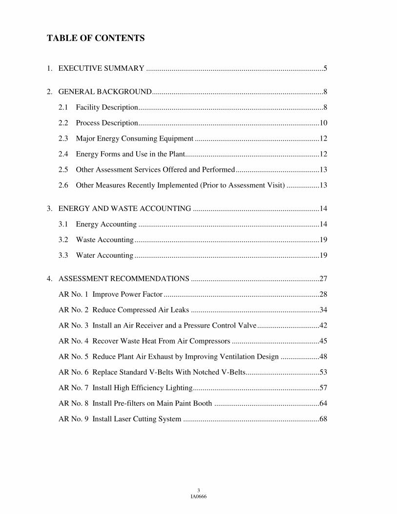
TABLE OF CONTENTS
1. EXECUTIVE SUMMARY ...........................................................................................5 2. GENERAL BACKGROUND........................................................................................8
2.1 Facility Description...............................................................................................8
2.2 Process Description.............................................................................................10
2.3 Major Energy Consuming Equipment ................................................................12
2.4 Energy Forms and Use in the Plant.....................................................................12
2.5 Other Assessment Services Offered and Performed...........................................13
2.6 Other Measures Recently Implemented (Prior to Assessment Visit) .................13 3. ENERGY AND WASTE ACCOUNTING .................................................................14
3.1 Energy Accounting .............................................................................................14
3.2 Waste Accounting...............................................................................................19
3.3 Water Accounting ...............................................................................................19 4. ASSESSMENT RECOMMENDATIONS ..................................................................27
AR No. 1 Improve Power Factor ................................................................................28
AR No. 2 Reduce Compressed Air Leaks ..................................................................34
AR No. 3 Install an Air Receiver and a Pressure Control Valve................................42
AR No. 4 Recover Waste Heat From Air Compressors .............................................45
AR No. 5 Reduce Plant Air Exhaust by Improving Ventilation Design ....................48
AR No. 6 Replace Standard V-Belts With Notched V-Belts......................................53
AR No. 7 Install High Efficiency Lighting.................................................................57
AR No. 8 Install Pre-filters on Main Paint Booth ......................................................64
AR No. 9 Install Laser Cutting System ......................................................................68

4 IA0666
5. ADDITIONAL ASSESSMENT ITEMS CONSIDERED...........................................73
5.1 Install Electronic Ballasts and T8 Lamps .............................................................73
5.2 Install Occupancy sensors.....................................................................................73
5.3 Install High Efficiency Motors .............................................................................74
6. RESOURCE DIRECTORY.........................................................................................75
6.1 State Programs ......................................................................................................75
6.2 National Resources ...............................................................................................75

5 IA0666
1. EXECUTIVE SUMMARY
Report No.: 666
S.I.C. No.: 3266 Location: Ames, IA Assessment Date: 04/01/05
Principal Products: Industrial Equipment
Annual production: 2,000 Annual Sales: $50 million
No. of Employees: 100 No. of ARs: 9
Estimated Cost of the Audit to the Client: 8 hours, $400
The cost saving opportunities that were evaluated for your facility are referred to as
Assessment Recommendations (ARs). This report describes nine assessment recommendations
which the audit team feels should be considered. The nine recommendations along with
potential cost saving, implementation cost, and simple payback are shown in Table 1.1.
Table 1.1 Summary of Assessment Recommendations Cost Savings
AR Description
Total Potential Cost
Savings ($/year)
Implementation Costs
($)
Simple Payback
1. Improve Power Factor 3,669 3,750 1.0 yr 2. Reduce Compressed Air Leaks 1,216 416 4 mo 3. Install an Air Receiver and a Pressure Control Valve 5,245 7,072 1.4 yr 4. Recover Waste Heat From Air Compressors 3,182 1,044 4 mo 5. Reduce Plant Air Exhaust by Improving Ventilation Design 12,016 2,495 3 mo 6. Replace Standard V-Belts With Notched V-Belts 528 136 4 mo 7. Install High Efficiency Lighting 1,628 - - 8. Install Pre-filters on Main Paint Booth 4,044 440 2 mo 9. Install Laser Cutting System 852,215 1,270,000 1.5 yr
Totals 883,743 1,285,353
The cost savings are based on reductions in energy usage, productivity improvement, and
waste minimization. Table 1.2 summarizes these values for each AR.

6 IA0666
Table 1.2 Summary of Assessment Recommendations Resource Savings
AR Description
Potential Electricity
Usage Savings (kWh/yr)
Potential Demand Savings
(kW-mo/yr)
Potential Natural
Gas Usage Savings
(MMBtu/yr)
Potential Labor
Reduct (hr/yr)
Primary Area*
Affected
1. Improve Power Factor - - - - P 2. Reduce Compressed Air Leaks 33,016 64.6 - -12 E 3. Install an Air Receiver and a Pressure Control Valve 63,700 420.0 - - E 4. Recover Waste Heat From Air Compressors - - 480 - E 5. Reduce Plant Air Exhaust by Improving Ventilation Design 11,658 22.8 1,725 - E 6. Replace Standard V-Belts With Notched V-Belts 7,890 34.8 - - E 7. Install High Efficiency Lighting 99,405 194.4 - - E 8. Install Pre-filters on Main Paint Booth - - - 80 P 9. Install Laser Cutting System - - - 2,080 P
Totals 215,669 736.6 2,314 2,148 * E = energy, W = waste, P = productivity
The energy consumption and corresponding costs at this facility from December 2002
through November 2003 are summarized in Table 1.3.
Table 1.3 Annual Energy Consumption and Corresponding Costs
Energy Source Billing Units MMBtu $
Electricity 1,982,400 kWh 6,765 130,953
Natural Gas 86,497 therms 8,651 61,881
Totals 15,416 192,834
The energy conservation ARs could save an estimated 2,941 MMBtu each year or 19.1% of
this plant’s total energy usage. The ARs could also save an estimated 736.6 kW-months of
demand each year, or 11% of the average monthly demand. The recommended productivity AR
could save 2,160 labor hours.
Comments
It should be noted that a "law of diminishing returns" applies to the total cost savings.
That is, the figures in Table 1.1 are based on the sum of the cost savings for each AR as if they
were independent. They are not; for example, if AR No. 3, Install an Air receiver and a Pressure
Control Valve, were implemented, the compressed air line pressure would be lower than at

7 IA0666
present and therefore, the magnitude of the air leaks and the cost savings to be realized by
implementing AR No. 2, Reduce Compressed Air Leaks, would be less than indicated above.
When deciding which recommended ARs to implement, AR interaction should be taken into
consideration.

8 IA0666
2. GENERAL BACKGROUND
2.1 Facility Description
The company considered in this report produces telescopic high-reach forklifts, which are
distributed internationally and nationally. Typically, 150 employees are involved in the
manufacturing of 1,650 units for an annual sales figure of approximately $120,000,000.
Approximate operating schedules of the various areas considered in this report are given in Table
2.1.
Table 2.1 Plant Operating Schedules
OPERATING SCHEDULE OF AREAS Area Operating
Schedule Days/wk Wk/yr Total hr/yr
Offices 7 a.m. to 5 p.m. Mon - Fri 52 2,600
Production 24 hr/day Mon - Thu 52 4,992
Production 7 a.m. to 11 p.m. Fri 52 832
Production 7 a.m. to 1 p.m. Sat 52 312
The facility is comprised of one building, with a total area of approximately 200,000 sq ft.
Most of the manufacturing processes are performed in the Production area. It is estimated that
4% of the building area is dedicated to office space. A simple layout of the facility is given in
Figure 2.1.
The building walls are constructed with a metal structure and 6” fiberglass insulated panels;
metal beams support the 6” fiberglass insulated roof. Only Offices are air-conditioned. Space
heating in the plant is done by natural gas burners at the makeup air units.

9 IA0666
Figure 2.1 Simple Facility Layout
Outdoor Testing Area
Offices
Welding Area
Painting Area Fabrication Area
Boom Assembly Area
Tractor Assembly Area
Final Assembly
Parts Storage
Pre-cut Metal Storage

10 IA0666
2.2 Process Description
A simplified description of the manufacturing processes performed at this facility is given
in this section. It is not intended to be a complete detailed description, but rather to provide
general information on the processes, with a focus on energy requirements and significant waste
streams.
This plant manufactures industrial equipment. Production begins with the arrival of pre-cut
steel, other raw materials, and assembly parts. Materials are delivered to the corresponding
storage area while assembly parts can go directly to the corresponding assembly area. Some
materials are placed on a short-term storage location. The main raw material is pre-cut steel
which is used to produce the telescopic boom and the chassis. The pre-cut steel is first finished
by machining processes, which include boring, chamfering, and forming. Then parts are pre-
assembled in jigs for welding. Manual welding or robotic welding completes the main parts.
Next, parts go for finishing, trimming and inspection. The final operation for making the parts is
painting, which is performed with an electrostatic liquid painting system, for which parts are
prepared either by blasting or by a phosphate wash. After inspection, parts go to the
corresponding assembly area All parts are finally assembled together in a separate area. All
equipments are tested for correct functioning before they are sent to the shipping area.
A process flowsheet, which shows the incoming and outgoing material streams of the
facility, is presented in Figure 2.2.

11 IA0666
Figure 2.2 Process Flowsheet
Receiving and
Storage
Pre-cut Steel
Receiving
Steel
Short Term Storage
Machining and Forming
Welding
Finishing
Painting
Final Assembly
Shipping
Controls
Paint
Parts Assembly
Parts Assembly
Testing
Seat

12 IA0666
2.3 Major Energy Consuming Equipment
The following list is an approximate summary of the major energy-consuming equipment
at this facility.
1. Electrical
A. Air Compressors (2) 100 hp Screw type unit, operating pressure at 110 psig (1) 25 hp Reciprocating unit, used as a Back-up
B. Major Process Related Equipment (32) welders, 15 kW each Several punch presses Several lathes, mills, drills, and folding presses C. HVAC (Heating, Ventilation and Air Conditioning) Fans Several extraction fans
Cooling (4) packaged air conditioning units, 62,000 Btu/hr each
D. Lighting 180 kW total estimated installed capacity
2. Natural Gas A. Major Process Related Equipment (1) paint drying booth, 2.0 MMBtu/hr
B. Space Heating (3) make up air units, 5.9 MMBtu/hr each
2.4 Energy Forms and Use in the Plant
Electrical energy is used for operating process-related equipment, lighting, compressing air,
and space cooling. Natural gas is used for paint drying and heating of the plant. No other energy
sources or fuels are consumed at this facility.

13 IA0666
2.5 Other Assessment Services Offered and Performed
According to facility personnel, no offers for assessments were made by other groups
within the last five years.
2.6 Other Measures Recently Implemented (Prior to Assessment Visit)
Some other significant energy conservation and waste minimization measures had been
implemented prior to the visit by the ISU assessment team, based on investigation and action by
facility personnel. These actions are summarized below.
2.6.1 Previous Waste Minimization Efforts
• Steel recycling
• Solvent recycling or disposal through licensed third party

14 IA0666
3. ENERGY AND WASTE ACCOUNTING
3.1 Energy Accounting
An essential component of any energy management program is a continuing account of
energy use and its corresponding cost. For energy, this can be developed by keeping up-to-date
records of energy consumption and associated costs on a monthly basis. When utility bills are
received, it is recommended that energy use and costs be recorded as soon as possible. A
separate record will be required for each type of energy used, i.e., gas, electric, oil, etc. A
combination will be necessary, for example, when both gas and oil are used interchangeably in a
boiler. A single energy unit should be used to express the heating values of the various fuel
sources so that a meaningful comparison of fuel types and fuel combinations can be made. The
energy unit used in this report for comparison is the Btu, British thermal unit, or million Btu’s
(MMBtu). The conversion factors are:
ENERGY CONVERSION FACTORS Unit Equivalent
1 MBtu 1,000 Btu 1 MMBtu 1,000,000 Btu 1 kWh 3,412 Btu 1 therm 100,000 Btu 1 hp-h (motor horsepower) 2,545 Btu 1 hp-h (boiler horsepower) 33,500 Btu 1 ton-h (refrigeration) 12,000 Btu
ENERGY CONTENT OF FUELS* Fuel Unit Energy Equivalent
1 cu ft natural gas 1,000 Btu 1 gallon No. 2 oil (diesel) 140,000 Btu 1 gallon No. 4 oil 145,000 Btu 1 gallon No. 5 oil 149,000 Btu 1 gallon No. 6 oil 150,000 Btu 1 gallon gasoline 130,000 Btu 1 gallon propane 92,000 Btu 1 ton coal 20,000,000 Btu
*varies with supplier

15 IA0666
The value of energy and cost records can be understood by examining those represented for
your facility on the following pages. The electrical energy usage and monthly demand are
tabulated by months in Table 3.1.1, and the natural gas energy usage in Table 3.1.2. Table 3.1.3
summarizes this information. Total annual energy usage and energy costs are shown in Figures
3.1.1 and 3.1.2. Figure 3.1.3 shows the annual electrical cost broken down as the total cost,
usage cost, demand cost, and other cost. A pie chart illustrating the percentage of energy use for
various functions is shown in Figure 3.1.4, and another pie chart illustrating the percentage of
energy costs for various functions is shown in Figure 3.1.5. From these figures, trends and
irregularities in energy usage and costs can be detected and the relative merits of energy
conservation and load management can be assessed.
In addition to plotting monthly energy consumption and cost, it may also be desirable to
plot the ratio of monthly energy consumption to monthly production. An appropriate measure of
production should be used consistent with the company's production record-keeping procedures.
The measure of production can be gross sales, number of units produced or processed, pounds of
raw material used, etc. It is important that the same time period be used for energy consumption
and production.
Marginal Costs
Economists define the marginal cost of a good as the price paid for one additional unit.
This concept is useful in energy calculation since the value of energy saved or the cost of
additional energy purchased will be at the marginal rate.
Marginal rates are almost always lower than average rates. There are two common reasons
for the difference. One is that fixed costs such as meter charges are usually constant each month
no matter how much energy is purchased. The other reason is that many utility companies
charge less per unit as the quantity purchased increases.

16 IA0666
Electricity Billing
The electrical usage and demand are tabulated in Table 3.1.1. The total electrical usage
and demand for each month is the sum of the usage and demand readings of the only electrical
meters at this facility. The usage cost is the sum of energy charges and the demand cost is the
sum of the billed demand charges. There is a flat rate throughout the day for either energy and
demand usage, i.e., there are not Peak hours defined. Other costs consist of all other charges that
do not depend on usage or demand. For this facility, other costs consist of the Sales Tax. The
total cost is simply the sum of all electrical costs.
The electric demand charges come from applying a fixed tiered billing structure, the first
100 kW are billed at one rate, the second 400 kW at a different rate, and the remainder kW at a
third rate. Every three months the utility company adjusts these rates.
The facility is billed extra charges if the average power factor (PF) is below 95%, which is
seen on the bills. If the power factor is above 95%, there are not extra charges. The low power
factor charge, LPF, can be calculated as:
LPF = [(demand) x (95%)/(PF) – (demand)] x (cost of first tier of demand)
For example, for the month of January , the plant’s demand was 529.2 kW with a power
factor of 89.4%, therefore the correction can be calculated as:
LPF = [(529.2) x (95%)/(89.4) – (529.2)] x ($8.07/kW)
LPF = $267.50
The marginal rate for electric energy, MRE, is the rate of the last kWh added to the bill in
the billing period. There are no different rates for different consumption levels. However, there
is a monthly Power Cost Adjustment that the utility company charges to recover the costs of the
fuel used to produce the electricity. The marginal rate for electricity is simply the quotient of the
summation of the energy costs by the number of kWh spent for each month. For the month of
December 2002, the marginal rate was calculated as:
MRE = [(Energy Cost) + (Power Cost Adjustment)] / (Energy Consumed)
Substituting values
MRE = [(3,073.04) + (1,877.67)] / (139,500)

17 IA0666
MRE = $0.0355/kWh
Electricity used in the plant is almost 68% of the cost but only 44% of the total energy usage.
Electric Bill Sample Calculation
The following is an example of the electric charges for this facility for the month of
December 2002: Billing Demand = 529.2 kW Energy Consumed = 135,900 kWh Demand Charges: 100 kW @ $8.07/kW = $807.00 400 kW @ $7.37/kW = $2,948.00 29.2 kW @ $6.67/kW = $194.76 Low Power Factor charges: LPF = $267.50 Energy Charges: 139,500 kWh @ $0.02203/kWh = $3,073.19 139,500 kWh @ $0.01346/kWh = $1,877.67 Other Costs: State Sales Tax = $550.08 Total Electric Charges:
Demand Charges + Energy Charges + LPF + Other Costs = $9,718.20
In order to calculate the marginal cost for demand usage, MCD, it is necessary to account
for the effect of the low power factor in the final bill as well as looking at the cost of the last kW
added to the billing demand. Following with the example, for the month of December 2002, the
marginal cost for demand can be estimated as:
MCD = (cost of last kW added) + [(95%)/(PF) – 1 ] x (First Tier Cost)
Substituting values,
MCD = ($6.67/kW) + [(95%)/(0.894) – 1 ] x ($8.07/kW)
MCD = $7.18/kW

18 IA0666
Natural Gas Billing
The natural gas usage is tabulated in Table 3.1.2. The total natural gas usage is tabulated
for the only meter for each month. The usage cost is the gas cost and the delivery charges.
Other costs consist of all other charges that do not depend on usage. For this facility, other costs
consist of basic service charge and sales tax. The total cost is simply the sum of all costs
associated with natural gas. There are no discounts for large quantity purchases. For the
determination of the yearly average marginal cost, a weighted average is calculated. Each
month’s marginal rate is weighted by the monthly gas therms consumed. Natural gas use for
heating the plant is 48% of the total energy usage but only 28% of the cost. Natural gas used for
the process is 8% of the total energy usage but only 4% of the cost.
Natural Gas Bill Sample Calculation
The following is an example of the natural gas charges for this facility for the month of
December 2002
Total Billed Usage = 1,368.7 MMBtu
Energy Charges:
1,368.7 MMBtu @ $4.7111/MMBtu = $6,448.08
Delivery Charges:
1,368.7 MMBtu @ $0.7201/MMBtu = $985.60
Other Costs:
Service Charges + State and Local Taxes = ($60.00) + (449.42) = $509.42
Total Natural Gas Charges:
Energy Charges + Other Costs = $7,943.10
The marginal rate for natural gas, MGC, for this month is simply the gas unitary cost plus
the unitary delivery charge:
MGC = (3.031) + (0.821) = $3.85/MMBtu

19 IA0666
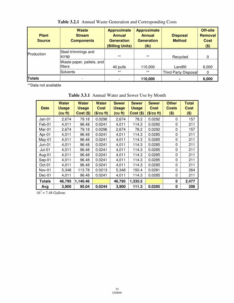
3.2 Waste Accounting
The manufacturing operations in this plant utilize various raw materials and produce
several waste streams. The values shown for the annual waste generation were found through
examination of monthly invoices for various waste streams and through discussions with plant
personnel on the day of the assessment.
Table 3.2.1 summarizes the waste streams at this facility and the costs associated with each
waste stream.
3.3 Water Accounting
The water consumption, sewer disposal and corresponding costs at this facility from
January 2003 through December 2003 are summarized in Table 3.3.1. The water usage cost and
sewer costs are calculated with different rates with their corresponding usage in cubic feet and
summed in the total cost column. Figure 3.3.1 shows the total annual water and sewer usage in
cubic feet. Al water usage pays sewer charges.
The costs for water and sewer are shown graphically in Figure 3.3.2. There are no other
costs other than direct costs for water and sewer usage. The sewer usage costs are higher than
the water usage costs. This fact is also evident in the pie chart, which graphically outlines the
percentages of costs.

20 IA0666
Table 3.1.1 Electric Energy Use by Month
Date Usage Usage Usage Demand Demand Other Total Marginal Marginal (kWh) (MMBtu) Cost ($) (kW) Cost ($) Cost ($) Cost ($) ($/kWh) ($/kW)
Dec-02 139,500 476 4,951 529 4,217 550 9,718 0.0355 7.18
Jan-03 177,300 605 6,164 597 4,738 654 11,556 0.0348 7.23
Feb-03 164,100 560 5,896 580 4,573 627 11,096 0.0359 7.15
Mar-03 155,700 531 5,618 541 4,275 593 10,486 0.0361 7.12
Apr-03 172,200 588 6,115 541 4,256 622 10,993 0.0355 7.09
May-03 171,900 587 6,111 533 4,109 614 10,834 0.0356 6.88
Jun-03 163,200 557 5,854 535 4,120 598 10,572 0.0359 6.92
Jul-03 168,300 574 6,130 606 4,615 644 11,389 0.0364 6.92
Aug-03 180,600 616 6,495 582 4,491 659 11,645 0.0360 6.96
Sep-03 159,300 544 5,852 584 4,486 621 10,959 0.0367 7.00
Oct-03 160,800 549 5,840 550 4,262 606 10,708 0.0363 6.99
Nov-03 169,500 578 6,129 542 4,245 623 10,997 0.0362 7.07
Total 1,982,400 6,765 71,155 N/A 52,387 7,411 130,953 N/A 84.52 Avg 165,200 564 5,930 560 4,366 618 10,913 0.0359 N/A
Table 3.1.2 Natural Gas Energy Use by Month
Date Usage Usage Usage Other Total Marginal (Therms) (MMBtu) Cost ($) Cost ($) Cost ($) ($/MMBtu)
Dec-02 13,687 1,369 7,434 509 7,943 5.43
Jan-03 23,813 2,381 14,975 1,280 16,255 6.29
Feb-03 16,924 1,692 12,678 824 13,502 7.49
Mar-03 7,001 700 6,328 447 6,775 9.04
Apr-03 2,496 250 1,525 155 1,680 6.11
May-03 1,390 139 948 120 1,068 6.82
Jun-03 735 74 552 97 649 7.51
Jul-03 728 73 524 95 619 7.20
Aug-03 710 71 453 91 544 6.38
Sep-03 1,380 138 899 118 1,017 6.52
Oct-03 5,776 578 3,503 273 3,776 6.06
Nov-03 11,857 1,186 7,537 516 8,053 6.36
Total 86,497 8,651 57,356 4,525 61,881 N/A Avg 7,208 721 4,780 377 5,157 6.63
Note: Marginal cost for Natural Gas Usage is based on a weighted average

21 IA0666
Table 3.1.3 Summary of Total Energy Usage
OVERALL ANNUAL
ENERGY & COST SUMMARY:
Total Energy = 15,416 MMBtu/yr
Total Cost = 192,834 $/yr
ENERGY END USES
Usage Type MMBtu % MMBtu Cost ($) % Cost
Cooling 203 1% 3,929 2%
Process Electric 6,562 43% 127,024 66%
Process Gas 1,211 8% 8,663 4%
Heating 7,440 48% 53,218 28%
Total 15,416 100% 192,834 100%
AVERAGE MARGINAL RATES
Electrical Usage = 0.0359 ($/kWh)
Electrical Usage = 10.52 ($/MMBtu)
Electrical Demand = 84.52 ($/kW-yr)
Natural Gas = 6.63 ($/MMBtu)

22 IA0666
0
500
1,000
1,500
2,000
2,500
3,000
Dec
-02
Jan-
03
Feb-
03
Mar
-03
Apr
-03
May
-03
Jun-
03
Jul-0
3
Aug
-03
Sep
-03
Oct
-03
Nov
-03
Ene
rgy,
MM
Btu
Figure 3.1.1 Annual Energy Usage
0
2,000
4,000
6,000
8,000
10,000
12,000
14,000
16,000
18,000
Dec
-02
Jan-
03
Feb-
03
Mar
-03
Apr
-03
May
-03
Jun-
03
Jul-0
3
Aug
-03
Sep
-03
Oct
-03
Nov
-03
Cos
t, $
Electricity Natural Gas
Figure 3.1.2 Annual Energy Costs

23 IA0666
0
2,000
4,000
6,000
8,000
10,000
12,000
14,000
Dec
-02
Jan-
03
Feb-
03
Mar
-03
Apr
-03
May
-03
Jun-
03
Jul-0
3
Aug
-03
Sep
-03
Oct
-03
Nov
-03
Cos
t, $
Total Usage Demand Other
Figure 3.1.3 Annual Electrical Costs

24 IA0666
Cooling1%
Process Electric43%Heating
48%
Process Gas8%
Figure 3.1.4 Percentage of Energy Usage
Cooling2%
Process Electric66%
Heating28%
Process Gas4%
Figure 3.1.5 Percentage of Energy Costs
25 IA0666
Table 3.2.1 Annual Waste Generation and Corresponding Costs
Waste Approximate Approximate Off-site Plant Stream Annual Annual Disposal Removal
Source Components Generation Generation Method Cost (Billing Units) (lb) ($)
Production Steel trimmings and scrap ** ** Recycled 0
Waste paper, pallets, and filters 40 pulls 110,000 Landfill 6,000
Solvents ** ** Third Party Disposal 0
Totals - - 110,000 - 6,000
**Data not available
Table 3.3.1 Annual Water and Sewer Use by Month
Water Water Water Sewer Sewer Sewer Other Total Date Usage Usage Cost Usage Usage Cost Costs Cost
(cu ft) Cost ($) ($/cu ft) (cu ft) Cost ($) ($/cu ft) ($) ($)
Jan-01 2,674 79.18 0.0296 2,674 78.2 0.0292 0 157 Feb-01 4,011 96.48 0.0241 4,011 114.3 0.0285 0 211 Mar-01 2,674 79.18 0.0296 2,674 78.2 0.0292 0 157 Apr-01 4,011 96.48 0.0241 4,011 114.3 0.0285 0 211 May-01 4,011 96.48 0.0241 4,011 114.3 0.0285 0 211 Jun-01 4,011 96.48 0.0241 4,011 114.3 0.0285 0 211 Jul-01 4,011 96.48 0.0241 4,011 114.3 0.0285 0 211 Aug-01 4,011 96.48 0.0241 4,011 114.3 0.0285 0 211 Sep-01 4,011 96.48 0.0241 4,011 114.3 0.0285 0 211 Oct-01 4,011 96.48 0.0241 4,011 114.3 0.0285 0 211 Nov-01 5,348 113.78 0.0213 5,348 150.4 0.0281 0 264 Dec-01 4,011 96.48 0.0241 4,011 114.3 0.0285 0 211
Totals 46,795 1,140.46 46,795 1,335.5 0 2,477 Avg 3,900 95.04 0.0244 3,900 111.3 0.0285 0 206
1ft3 = 7.48 Gallons

26 IA0666
0
1,000
2,000
3,000
4,000
5,000
6,000
Jan-
01
Feb-
01
Mar
-01
Apr
-01
May
-01
Jun-
01
Jul-0
1
Aug
-01
Sep
-01
Oct
-01
Nov
-01
Dec
-01
Wat
er U
se, c
f
Water Sewer
Figure 3.3.1 Annual Water and Sewer Usage
0
20
40
60
80
100
120
140
160
Jan-
01
Feb-
01
Mar
-01
Apr
-01
May
-01
Jun-
01
Jul-0
1
Aug
-01
Sep
-01
Oct
-01
Nov
-01
Dec
-01
Cos
t, $
Water Sewer Other
Figure 3.3.2 Annual Water and Sewer Costs

27 IA0666
4. ASSESSMENT RECOMMENDATIONS
The following sections describe each of the assessment recommendations for this facility.
Included in each discussion is a summary of the recommended action, a background description,
the calculation of anticipated savings, and an estimate of the implementation cost. Finally, it
should be noted that, in general, these recommendations do not take into account any possible
future savings attributed to such things as changing rates and/or regulations.

28 IA0666
AR No. 1 - Improve Power Factor Recommended Action
Install capacitors to correct for low power factor.
Estimated Cost Savings = $3,699/yr
Estimated Implementation Cost = $3,750
Simple Payback = 1 year Background
Power factor is a way of quantifying the reaction of alternating current (AC) electricity to
various types of electrical loads. Inductive loads, such as motors and fluorescent lamp ballasts, cause
the voltage and current to shift out of phase. The utility company must supply additional power,
measured in kilovolt-amps (kVA), to make up for the phase shift. The total power requirement of the
load is made up of two components, the resistive, or real, component and the reactive component.
The resistive component, measured in kilowatts (kW) by a watt meter, does the useful work. The
reactive component, measured in reactive kilovolt-amps (kVAR), represents the current needed to
produce the magnetic field for the operation of a motor or other inductive device. This component
does no useful work, is not registered on a power meter, but contributes to the heating of generators,
transformers and transmission lines, constituting a loss for the utility company.
The ratio of real, usable power (kW) to apparent power (kVA) is known as the power
factor. To reduce reactive losses, the user should increase the power factor to a value as close to
unity (1.0) as is practical for the entire manufacturing plant. The utility supplying electricity to
this facility assesses a power factor charge when the power factor falls below a specified level
because more apparent power must be supplied as the user's power factor decreases.

29 IA0666
Figure 4.1.1 Components of Electrical Power
For example, it is assumed that a manufacturing plant has an average annual power factor of
0.78. A power factor of 0.78 means that for every 78 kW of usable power that the plant requires,
the utility must supply 78 kW/(PF) or 100 kVA. If the plant's power factor is changed from 0.78
to 0.95, then for every 78 kW required by the plant, the utility needs only to supply 78 kW/0.95 or
82 kVA.
The utility supplying electricity to this facility assesses a power factor charge when the
power factor is below 95%. This charge is often accomplished by increasing the billing demand
(kW) by 1% for each 1% by which the power factor is less than 95%.
Capacitor banks can be installed to decrease the reactive power (kVAR) and thus the
apparent power. Capacitors draw current that leads the voltage, while inductive loads draw
current that lags the voltage. The net result is that the current in the supply line is brought more
closely in phase with the supply voltage. A power factor of 1.0 indicates that the current and the
voltage are exactly in phase.
30 IA0666
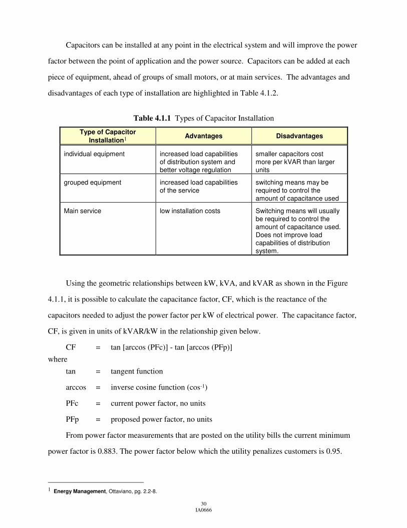
Capacitors can be installed at any point in the electrical system and will improve the power
factor between the point of application and the power source. Capacitors can be added at each
piece of equipment, ahead of groups of small motors, or at main services. The advantages and
disadvantages of each type of installation are highlighted in Table 4.1.2.
Table 4.1.1 Types of Capacitor Installation
Type of Capacitor Installation1
Advantages Disadvantages
individual equipment increased load capabilities of distribution system and better voltage regulation
smaller capacitors cost more per kVAR than larger units
grouped equipment increased load capabilities of the service
switching means may be required to control the amount of capacitance used
Main service low installation costs Switching means will usually be required to control the amount of capacitance used. Does not improve load capabilities of distribution system.
Using the geometric relationships between kW, kVA, and kVAR as shown in the Figure
4.1.1, it is possible to calculate the capacitance factor, CF, which is the reactance of the
capacitors needed to adjust the power factor per kW of electrical power. The capacitance factor,
CF, is given in units of kVAR/kW in the relationship given below.
CF = tan [arccos (PFc)] - tan [arccos (PFp)] where tan = tangent function
arccos = inverse cosine function (cos-1)
PFc = current power factor, no units
PFp = proposed power factor, no units
From power factor measurements that are posted on the utility bills the current minimum
power factor is 0.883. The power factor below which the utility penalizes customers is 0.95.
1 Energy Management, Ottaviano, pg. 2.2-8.

31 IA0666
Thus, the kVAR/kW of capacitors needed to avoid power factor charges can be computed as
follows:
CF = tan [arccos (0.883)] - tan [arccos (0.95)]
CF = 0.203 kVAR/kW
Table 4.1.2, generated from the above equation, provides the capacitance factor that can be
used to determine the amount of capacitance required to correct from an existing to a desired
power factor. The number in the table is multiplied by the current demand (kW) to get the
amount of capacitors (kVAR) needed to correct from the existing to the desired power factor.
Table 4.1.2 Power Factor Correction
Existing Power Corrected Power Factor
Factor 1.00 0.95 0.90 0.85 0.80 0.75 0.66 1.138 0.810 0.654 0.519 0.388 0.256 0.68 1.078 0.750 0.594 0.459 0.328 0.196 0.70 1.020 0.692 0.536 0.400 0.270 0.138 0.72 0.964 0.635 0.480 0.344 0.214 0.082 0.74 0.909 0.580 0.425 0.289 0.159 0.027 0.76 0.855 0.526 0.371 0.235 0.105 0.78 0.802 0.474 0.318 0.183 0.052 0.80 0.750 0.421 0.266 0.130 0.82 0.698 0.369 0.214 0.078 0.84 0.646 0.317 0.162 0.026 0.86 0.593 0.265 0.109 0.88 0.540 0.211 0.055 0.90 0.484 0.156 0.92 0.426 0.097 0.94 0.363 0.034 0.96 0.292 0.98 0.203 0.99 0.142
For this facility, the maximum monthly demand load during the previous year is
approximately 606 kW. The power factor correction as calculated above is 0.203. Table 4.1.2
can also be used to determine the amount of capacitors needed to correct this power factor to
95% where there would be no power factor charge. The amount of capacitors needed, kVAR,
can now be determined:
kVAR = (D) x (CF)

32 IA0666
where D = maximum annual demand, kW
CF = correction factor, as calculated above or read from table, kVAR/kW Therefore, kVAR = (606) x (0.203) = 123 kVAR � 125 kVAR
The cost savings can be calculated by multiplying the demand cost by the increased
demand due to low power factor for each month, as follows:
CS = (Dpf) x (demand cost)
The increased billing demand due to low power factor, Dpf, is estimated as:
Dpf = {(D) x [ (PFp) / (PFc) ]} – (D) where D = measured peak demand for the month, kW
PFp = minimum power factor necessary to avoid power factor charges, no units
PFc = current power factor, no units
As an example for your facility, the cost due to low power factor in December 2002 is found as:
Dpf = {(529.2) [ (0.95) / (0.894) ]} – (529.2)
Dpf = 33.14 kW
Following with the substitutions,
CSDec = (33.14) (8.07) = $268
Table 4.1.3 details the potential cost savings. The total cost savings for the year analyzed would
be:
CS = $3,699/yr

33 IA0666
Table 4.1.3 Summary of Cost Savings
Month
Power Factor
Demand
(kW) Cost
($/kW) CS ($)
Dec-02 0.8940 529.2 8.07 268 Jan-03 0.8880 597.0 8.07 336 Feb-03 0.8882 579.6 7.99 322 Mar-03 0.8906 541.2 7.99 288 Apr-03 0.8938 540.9 7.99 272 May-03 0.8910 533.1 7.77 274 Jun-03 0.8871 534.6 7.77 295 Jul-03 0.8870 606.0 7.77 334 Aug-03 0.8830 581.7 7.81 345 Sep-03 0.8866 583.5 7.81 326 Oct-03 0.8843 549.6 7.81 319 Nov-03 0.8839 542.4 7.88 320
Total 3,699
Implementation Cost
As calculated on the previous page, the installation of capacitors rated at 125 kVAR would
be required to correct for low power factor. The installation of these capacitors should increase
the power factor to the desired level of 95%. With this improved power factor there would be no
power factor charge. The installed cost for capacitors is estimated as $30/kVAR, and therefore
the implementation cost, IC, is estimated as:
IC = (125 kVAR) ($30/kVAR) = $3,750
Therefore, the annual cost savings of $3,699/yr would pay for the implementation cost of
$3,750 within 1 year. To determine the exact optimum power correction factor and the
specification of the capacitors requires engineering work beyond the scope of this report. It is
recommended that additional professional advice be obtained from a capacitor supplier or an
engineering firm. Finally, note that no energy savings can be attributed to this action; the
savings are strictly monetary.

34 IA0666
AR No. 2 - Reduce Compressed Air Leaks Recommended Action
Repair leaks in compressed air lines on a regular basis.
Estimated Electrical Demand Savings = 5.38 kW-mo/yr or 64.6 kW-mo/yr
Estimated Electrical Energy Savings = 33,016 kWh/yr
Estimated Electrical Demand Cost Savings = $455/yr
Estimated Electrical Energy Cost Savings = $1,181/yr
Estimated Net Cost Savings = $1,216/yr
Estimated Implementation Cost = $416
Simple Payback = 4 months Background
Compressed air is sometimes referred to as the most expensive "utility" in a plant. Air
compressors can consume a great deal of electrical energy and contribute significantly to electric
demand. Blow-offs using compressed air and avoidable air leaks are therefore quite costly.
Repairing even small leaks can lead to significant savings. The following table lists the various
air compressors at this facility and the operating conditions.
Table 4.2.1 Compressor Operating Conditions
Compressor #
Compressor Type Motor Size Operating Pressure
1 Screw 100 hp 110
2 Screw 100 hp 110
3 Reciprocating 25 hp Back-up
On the day of the audit, specific leaks were located and tagged in the facility. These
locations are summarized in Table 4.2.2.
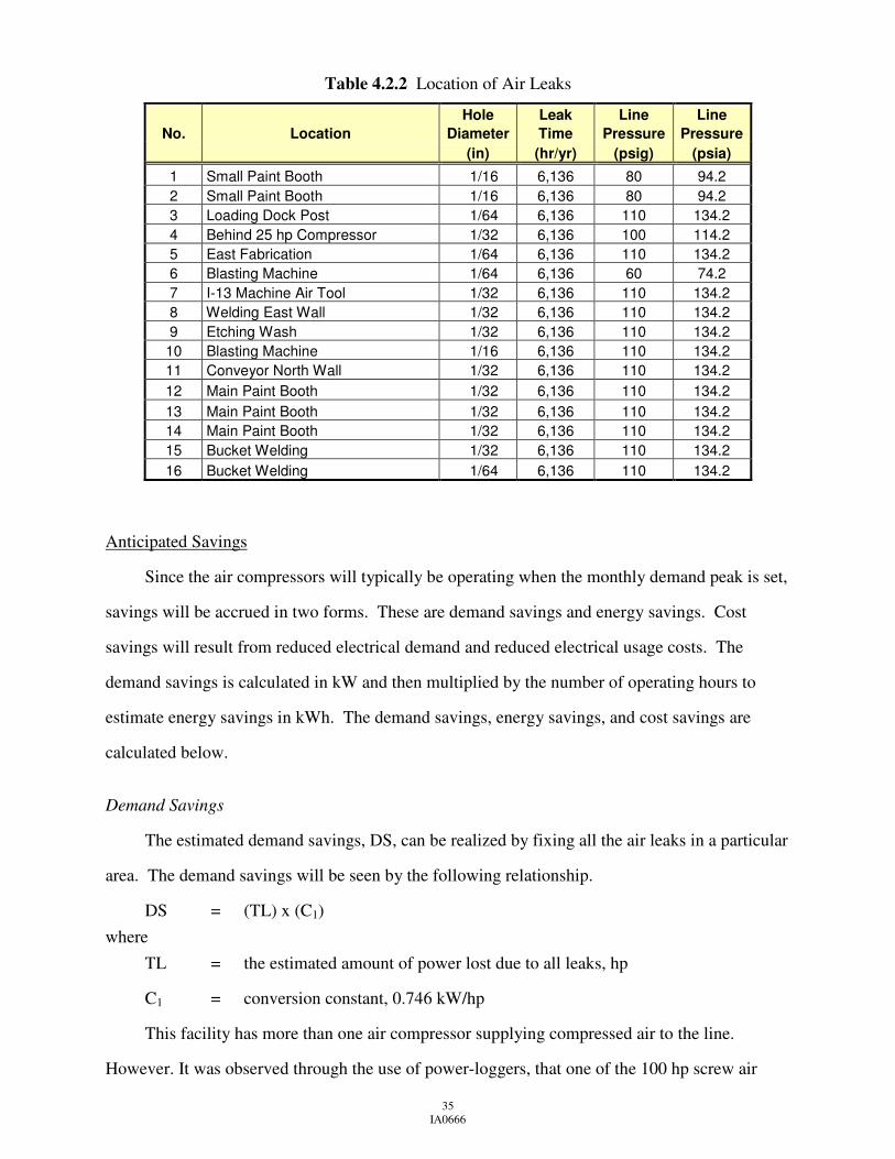
35 IA0666
Table 4.2.2 Location of Air Leaks
Hole Leak Line Line No. Location Diameter Time Pressure Pressure
(in) (hr/yr) (psig) (psia)
1 Small Paint Booth 1/16 6,136 80 94.2 2 Small Paint Booth 1/16 6,136 80 94.2 3 Loading Dock Post 1/64 6,136 110 134.2 4 Behind 25 hp Compressor 1/32 6,136 100 114.2 5 East Fabrication 1/64 6,136 110 134.2 6 Blasting Machine 1/64 6,136 60 74.2 7 I-13 Machine Air Tool 1/32 6,136 110 134.2 8 Welding East Wall 1/32 6,136 110 134.2 9 Etching Wash 1/32 6,136 110 134.2 10 Blasting Machine 1/16 6,136 110 134.2 11 Conveyor North Wall 1/32 6,136 110 134.2 12 Main Paint Booth 1/32 6,136 110 134.2 13 Main Paint Booth 1/32 6,136 110 134.2 14 Main Paint Booth 1/32 6,136 110 134.2 15 Bucket Welding 1/32 6,136 110 134.2 16 Bucket Welding 1/64 6,136 110 134.2
Anticipated Savings
Since the air compressors will typically be operating when the monthly demand peak is set,
savings will be accrued in two forms. These are demand savings and energy savings. Cost
savings will result from reduced electrical demand and reduced electrical usage costs. The
demand savings is calculated in kW and then multiplied by the number of operating hours to
estimate energy savings in kWh. The demand savings, energy savings, and cost savings are
calculated below.
Demand Savings
The estimated demand savings, DS, can be realized by fixing all the air leaks in a particular
area. The demand savings will be seen by the following relationship.
DS = (TL) x (C1) where TL = the estimated amount of power lost due to all leaks, hp
C1 = conversion constant, 0.746 kW/hp
This facility has more than one air compressor supplying compressed air to the line.
However. It was observed through the use of power-loggers, that one of the 100 hp screw air

36 IA0666
compressor was responsible for almost 100% of the compressed air production. As a result, only
one compressor was considered in the analysis. As both 100 hp screw air compressors are
identical, it does not affects the results whichever is in use.
The volumetric flow rate of free air, V, exiting the hole is dependent upon whether the
flow is choked. When the ratio of atmospheric pressure to line pressure, Patm/Pline, is less than
0.5283, the flow is said to be choked (i.e. it is traveling at the speed of sound). The volumetric
flow rate of free air, V, exiting the leak under choked flow conditions is calculated as follows:
Vj = (Tin + 460) x (
PlinejPatm ) x (C4) x (C5) x (C6) x (Cd) x (
Dj2
4 ) x (PI)
(Tline + 460)0.5
where Tin = temperature of the air at the inlet of compressor “i”, °F
Plinej = line pressure at leak “j”, psia
Patm = atmospheric pressure, 14.2 psia (based on 1,000 ft above sea level)
C4 = isentropic sonic volumetric flow constant, 28.37 ft/sec-°R0.5
C5 = conversion constant, 60 sec/min
C6 = conversion constant, 1/144 ft2/in2
Cd = coefficient of discharge for square edged orifice, 0.8 no units2
Dj = leak diameter, in
PI = π, 3.1416
Tline = average line temperature, °F
Thus, the volumetric flow rate of air exiting the leak at the Small Paint Booth area that can
be contributed to the 100 hp screw air compressor is:
V1 = (85 + 460) (
94.214.2 ) (28.37) (60) (
1144 ) (0.8) (
0.06252
4 ) (3.1416)
( 75 + 460)0.5
V1 = 4.53 cfm
In order to calculate the power loss from each leak, each volume component must be
evaluated separately, and then summed together. The power loss from each component, Lj, is
2 A.H. Shapiro, The Dynamics and Thermodynamics of Compressible Fluid Flow, Vol. 1, Ronald Press, N.Y. 1953, p. 100.

37 IA0666
estimated as the power required to compress the volume of air lost, VL, from atmospheric
pressure, Patm, to the compressor discharge pressure, Po, as follows3,4:
Lj = (Patm) x (C2) x (Vi) x [
(k)(k − 1) ] x (N) x (C3) x { [
(Po)(Patm) ] [
(k − 1)
(k x N) ] − 1 }
(Eai) x (Emi)
where
C2 = conversion constant, 144 in2/ft2
k = specific heat ratio of air, 1.4, no units
N = number of stages of compressor “i”, no units
C3 = conversion constant, 3.03 x 10⁻⁵ hp-min/ft-lb
Po = compressor operating pressure, psia
Ea = air compressor isentropic (adiabatic) efficiency5, no units (0.82 for rotary screw compressors)
Em = compressor motor efficiency, no units
The power loss component for the leak found at the Small Paint Booth area can now be
calculated as:
L1 = (14.2) (144) (4.53) [
(1.4)(1.4 − 1) ] (1) (3.03 x 10⁻⁵) { [
(124.2)(14.2) ] [
(1.4 − 1)
(1.4 x 1) ] − 1 }
(0.82) (0.936)
L1 = 1.10 hp
The demand savings, DS1, from the air leak found in the Paint Booth (shipping) area will
be:
DS1 = (TL1) x (0.746 kW/hp)
DS1 = (1.10) (0.746)
DS1 = 0.82 kW
From Table 4.2.3, it is seen that the total estimated monthly demand savings, found from
summing the demand savings for each leak, is:
3 Chapters 10 and 11, Compressed Air and Gas Handbook, Fifth Edition, Compressed Air and Gas Institute, New Jersey, 1989. 3 Gibbs, Charles W. ed. Compressed Air and Gas Data, Ingersoll-Rand Company, New Jersey, 1971. 5 From Table 1, p. 49, Pneumatic Handbook, 7th ed., Antony Barber, Trade and Technical Press, 1989.

38 IA0666
DS = 5.38 kW
Energy Savings
The energy savings realized by repairing air leaks, ES, can be calculated as follows:
ES = (DS) x (H) where H = operating hours of the compressor in each area, hr/yr
Therefore, the savings associated with the Small Paint Booth will be:
ES1 = (0.82) (6,136)
ES1 = 5,032 kWh/yr
Table 4.2.3 describes the savings associated with fixing the air leaks. The total estimated
energy savings, ES, can be found in Table 4.2.3 as:
ES = 33,016 kWh/yr Cost Savings
The annual cost savings, CSi, associated with each leak can be estimated as follows:
CSi = (ECSi) + (DCSi)
where
ECSi = energy cost savings, $/yr
DCSi = demand cost savings, $/yr
The energy cost savings can be calculated as follows:
ECSi = (ESi) x (unit usage cost, $/kWh)
ECSi = (5,032 kWh/yr) ($0.0359/kWh)
ECSi = $181/yr
The total estimated annual energy cost savings , ECS, can be found in Table 4.2.3 as:
ECS = $1,181/yr
And the demand cost savings can be calculated as:
DCSi = (DSi) x (unit demand cost, $/kW-yr)
DCSi = (0.82 kW) ($84.52/kW-yr)
DCSi = $69/yr

39 IA0666
The total estimated annual demand cost savings , CS, can be found in Table 4.2.3 as:
DCS = $455/yr
Substituting values,
CSi = (181) + (69)
CSi = $250/yr
The total estimated annual cost savings, CS, can be found in Table 4.2.3 as:
CS = $1,636/yr
Increased Costs
Inspecting the compressed air system and detecting leaks has a cost associated. It is
recommended on a regular basis to conduct an air leak detection survey. The period between
surveys cannot be determined due to the fact that it cannot be predicted how many air leaks will
be found. It is recommended to continue with inspections once a year, during the yearly plant
shut down, and adjust the period between surveys according to results. Also, plant personnel
should be encouraged to report leaks if discovered, and corrective actions could be scheduled. It
is assumed that for this facility, a crew of two people would be able to inspect the compressed air
system in six ours.
So, the increased costs, IC, can be estimated as:
IC = (N) x (HS) x (LC)
where
N = number of inspectors, person
HS = hours to conduct the survey, hr/yr
LC = labor cost, $/hr
Substituting values:
IC = (2) x (6) x (35)
IC = $420/yr
Finally, the net cost savings, NCS, for implementing this recommendation, are estimated
by the following equation:

40 IA0666
NCS = (ECS) + (DCS) – (IC)
Substituting values,
NCS = (1,181) + (455) – ($420/yr)
NCS = $1,216/yr
Table 4.2.3 also gives the volumetric flow rate, power lost due to the leak, energy and
demand savings and total cost savings for fixing the leaks.
Table 4.2.3 Cost of Compressed Air Leaks
Volumetric Power Demand Energy Demand Energy Total No. flow rate Loss Savings Savings Savings Savings Savings
(cfm) (hp) (kW) (kWh/yr) ($/yr) ($/yr) ($/yr)
1 0.00 1.10 0.82 5,032 69 181 250 2 4.53 1.10 0.82 5,032 69 181 250 3 0.37 0.09 0.07 430 6 15 21 4 1.37 0.33 0.25 1,534 21 55 76 5 0.37 0.09 0.07 430 6 15 21 6 0.22 0.05 0.04 245 3 9 12 7 1.49 0.36 0.27 1,657 23 59 82 8 1.49 0.36 0.27 1,657 23 59 82 9 1.49 0.36 0.27 1,657 23 59 82 10 5.98 1.45 1.08 6,627 91 238 329 11 1.49 0.36 0.27 1,657 23 59 82 12 1.49 0.36 0.27 1,657 23 59 82 13 1.49 0.36 0.27 1,657 23 59 82 14 1.49 0.36 0.27 1,657 23 59 82 15 1.49 0.36 0.27 1,657 23 59 82 16 0.37 0.09 0.07 430 6 15 21
7.18 5.38 33,016 455 1,181 1,636
From Table 4.2.3, it can be seen that the cost of compressed air leaks increases as the size
of the leak increases. This fact can be seen even more clearly in the following air leak graph,
Figure 4.2.1. Figure 4.2.1 is based upon the operating conditions for this facility including the
energy costs, line pressure, and operating hours. As part of a continuing program to find and
repair compressed air leaks, this graph can be referenced to estimate the cost of any leaks that
may be found.

41 IA0666
0
1,500
3,000
4,500
6,000
7,500
9,000
0 1/ 32 1/ 16 3/ 32 1/ 8 5/ 32 3/ 16 7/ 32 1/ 4 9/ 32 5/ 16 11/ 32 3/ 8
Air Leak Diameter, in
Yea
rly
Los
ses,
$/yr
$0.03590
110.0
6,136
Energy Cost, $/kWh =
Line Pressure, psig =
Operating Hours, hr/yr =
Operating Conditions
Demand Cost, $/kW-yr = $84.52
Figure 4.2.1 Cost of Energy Losses Due to Air Leaks Implementation Cost
Implementation of this AR will involve repairing the air leaks found in the facility. The
cost estimate for materials needed in these repairs is found from the 2000-2001 Grainger
General Catalog and are shown in Table 4.2.4.
Table 4.2.4 Materials Costs for Air Leak Repairs
Description Unit Price ($) Number of Units Total ($)
200 psi General purpose hose 94.00/(100 ft length) 1 94
Coupling 6.00 ea 7 42
Total 136
It is estimated that two air leaks could be repaired in one hour. Thus, the 16 leaks could be
repaired in approximately 8 hours at a labor cost of $35/hr. The annual net cost savings of
$1,216/yr will pay for the estimated implementation cost of $416 within 4 months.

42 IA0666
AR No. 3 – Install an Air Receiver and a Pressure Control Valve
Recommended Action
Install an air receiver (surge tank) in the compressed air system and a pressure control
valve. This can eliminate the use of the second compressor.
Estimated Electrical Demand Savings = 35.0 kW each month, or 420.0 kW-mo/yr
Estimated Electrical Energy Savings = 63,700 kWh/yr
Estimated Cost Savings = $5,245/yr
Estimated Implementation Cost = $7,072
Simple Payback Period = 1.4 years
Background
Receivers are usually a necessary part of a Compressed Air System. Adding more
compressed air storage decreases the number of times a compressor must alternate between
loaded and unloaded states. In addition, the receiver provides a buffer of air for the system. This
buffer allows peaks in the load to be supplied by air from the receiver and hence avoiding an
additional compressor to get into service, as well as assuring all equipments fed by the system
always have acceptable pressure levels for operation.
Normally at this facility, a lead 100 hp screw air compressor runs the entire shifts, while a
secondary 100 hp screw air compressor runs during moments of peaks in consumption. The
second compressor operates approximately for six hours unloaded every day, and about an hour
supplying air to the line. The installation of the receiver tank could allow the lead compressor to
successfully carry the entire load every day.
In addition, it is recommended a constant pressure valve be installed after the receiver. As
significant amount of compressed air is being used in air leaks and blow-offs, limiting the
pressure of the system automatically limits the amount of air lost in leaks or other loads
dependant on line pressure.

43 IA0666
Anticipated Savings
The secondary 100 hp screw air compressor contributes to the demand reading, therefore
savings will accrue from the decrease in monthly demand and the decrease in annual energy
usage. The demand savings are calculated in kW and then multiplied by the number of operating
hours to get energy savings in kWh. The demand savings, energy savings and cost savings are
calculated below.
Demand Savings
The annual demand savings, DS, after the receiver has been installed can be estimated as
follows:
DS = (DU) where DU = demand when compressor is unloaded, kW
The demand contribution when the compressor is unloaded was measured with power
loggers on the day of the audit. As the secondary compressor runs unloaded for at least 15
minutes before being automatically shut off, the demand contribution is just the unloaded power.
DS = (35)
DS = 35 kW
Energy Savings
The annual energy savings that could be realized by avoiding the use of the secondary
compressor, ES, can be estimated by the following equation:
ES = (DS) x (H)
Where
H = secondary compressor operational yearly hours, hr/yr
H = (7 hr/day) x (5 day/week) x (52 week/yr)
H = 1,820 hr/yr
Following through with the previous calculation,
ES = (35) x (1,820)

44 IA0666
ES = 63,700 kWh/yr
Electrical Cost Savings
Annual electrical cost savings, ECS, for the 40 hp compressor is estimated as:
ECS = [ (DS) x (unit cost of demand) ] + [ (ES) x (unit cost of electricity) ]
ECS = [ (35 kW) x ($84.52/kW-yr) ] + [ (63,700 kWh/yr) x ($0.0359/kWh) ]
ECS = $5,245/yr
Implementation Costs
Implementing this measure will require purchasing and installing a receiver (surge tank).
The receiver size that would be needed is estimated in 1,000 gallons. The costs associated with
purchasing and installing this size receiver are broken down in Table 4.3.1.
Table 4.3.1 Materials Costs for Installing a Receiver and a Pressure Control Valve
Description Unit Price ($) Number of Units Total ($)
1,000 gallons receiver 3,000 1 3,000
1” relief valve 72 1 72
3” flow pressure control valve 750 1 750
miscellaneous materials 800 1 800
Delivery of materials 350 1 350
Total 4,972
It is estimated that 60 hours of labor would be necessary to install the receiver, at a labor
cost of $35/hr result in a total labor cost of $2,100. The total implementation cost of the project
is $7,072. The annual savings of $5,245 would pay for the implementation cost within 1.4 years.

45 IA0666
AR No. 4 - Recover Waste Heat From Air Compressors
Install ductwork to allow warm air from the air compressors outlet to be used to
supplement the plant heating load for neighboring areas of the plant.
Estimated Energy Savings = 480 MMBtu/yr
Estimated Cost Savings = $3,182/yr
Estimated Implementation Cost = $1,044
Simple Payback Period = 4 months
Background
Presently, waste heat from the air compressor is discharged outside. By installing
additional ductwork, the compressor waste heat would be available to heat the other areas in the
plant. During the months when heating is not required, the heat from the compressor should still
be ducted to the outside so no additional heating loads are added which will warm the plant. A
simple damper in the ductwork can be used to switch from a cooling to heating season setting.
Anticipated Savings
By recovering the heat lost from the air compressor and using it to supplement the natural
gas heaters in the plant, an energy savings, ES, will accrue due to the decrease in natural gas
used in the existing heaters. By using less gas and therefore less energy, a cost savings, CS, will
occur. The procedure used here calculates the rate of heat loss in MMBtu per hour and then
multiplies by the seasonal operating hours to get the savings in MMBtu. The energy savings and
cost savings are calculated below.
Energy Savings
It is estimated that typically screw compressors can have about 60% of their energy
recovered in the form of heat. On the day of the audit, power measurements taken for the 100 hp

46 IA0666
screw air compressor indicated an average power requirement of 75 kW. Thus, a simple
calculation can estimate the amount of energy that can be recovered.
Q = (D) x (H) x (FHR)
where,
D = average demand of the compressor, 80 kW
H = estimated hours when heat recovery is plausible, h/yr
FHR = fraction of heat available for recovery, no units
Thus, the total amount of energy recovered is:
Q = (75) x (2,500) x (0.60)
Q = 112,500 kWh/yr
The rate of heat loss from the compressor is the total heat added to the plant by the
compressor. Given this information, the natural gas energy savings from the heat added to the
plant each year can be estimated as:
ES = (Q) x (C1) x (C2) / (Eff)
where,
C1 = conversion constant, 3,412 Btu/kWh
C2 = conversion constant, 10-6 MMBtu/Btu
Eff = efficiency of the heating system, no units
Substituting values,
ES = (112,500) x (3,412) x (10-6) / (0.80)
ES = 480 MMBtu/yr
Costs Savings
The annual energy cost savings for the decreased use of the natural gas heaters, ECS, is
calculated as follows:
ECS = (ES) x (marginal unit usage cost of gas $/MMBtu)
ECS = (480) x (6.63)
ECS = $3,182/yr

47 IA0666
There will not be significant additional operation cost associated with the proposed
installation. The existing compressor fan would be able to force the air into the plant.
Implementation Cost
Sheet metal ductwork would be easily used to move the waste heat from the compressor
outlet to the rest of the plant. The total implementation cost for material and labor to make this
modification to the compressor room is broken down in Table 4.4.1.
Table 4.4.1 Costs for Implementing the Ductwork
Description Unit Cost # of Units Total ($)
Damper $157 ea 2 314 Duct 3'x5' $20/ft 5 100 Labor $35/hr 18 630
Total: 1,044
The annual cost savings of $3,182/yr will pay for the implementation cost of $1,044 within 4
months.

48 IA0666
AR No. 5 – Reduce Plant Air Exhaust by Improving Ventilation Design
Recommended Action
Add a 16,000 cfm fan at a convenient location and avoid using one of the 32,600 cfm
exhaust fan. This action would reduce the overall electrical energy and demand requirements,
and reduce the gas usage for heating of the plant.
Estimated Electrical Demand Savings = 1.9 kW each month, or 22.8 kW-month/yr
Estimated Electrical Energy Savings = 11,658 kWh/yr
Estimated Gas Usage Savings = 1,725 MMBtu/yr
Estimated Cost Savings = $12,016/yr
Estimated Implementation Cost = $2,495
Simple Payback = 3 months
Background
The existing plant ventilation system has eleven 5 hp air exhaust fans (32,600 cfm), and
two 1.5 hp air exhaust fans(10,600 cfm). The amount of air drawn from the plant is controlled
manually by choosing which exhaust fans should be in operation. Normally, several of the 5 hp
fans and the two 1.5 hp fans operate. According to the activity on the plant, and in order to
evacuate fumes generated at the Welding area, additional fans are brought into service. On the
day of the audit, it was observed that the locations of the fans do not favor the air circulation
from the “clean” areas to the Welding area. Actually, it causes a path for fumes to move into the
“clean” areas such as Fabrication, Boom Assembly, and Tractor Assembly. The problem is fixed
by exhausting more air from these areas while creating even more conditions for the fumes to be
driven into these areas.
It is recommended to perform a detailed ventilation study, which would probably result in
the addition of new exhaust fans at more convenient locations. For estimating the savings from
implementing this recommendation, it is assumed that by installing a 2 hp air exhaust fan (
16,000 cfm) at a convenient location, one of the 5 hp air exhaust fans ( 32,600 cfm) would not be

49 IA0666
used. This would reduce the demand and energy used by the ventilation system and also reduce
the amount of plant air being exhausted. As a consequence, the heating energy that must be used
to condition the outdoor air which makes up the exhaust would be reduced.
Anticipated Savings
The anticipated savings for the recommendation would be accrued in three forms: electric
demand savings, electric energy savings, and gas usage savings with the associated cost savings.
Demand Savings
The calculations are based on the required power by the different motor sizes. The demand
savings, DS, for the smaller fan motor can be estimated using the following relationship:
DS = (CD) – (PD)
where:
CD = the current demand of a 5 hp motor, kW
PD = the proposed demand of a 2 hp motor, kW
The current demand, CD, can be estimated as follows:
CD = (HP) x (C1) x (LF) / (EFF)
where
HP = motor horsepower, hp
C1 = conversion constant, 0.746 kW/hp
LF = load factor, no units
EFF = efficiency of fan motor, no units
Substituting values:
CD = [(5) x (0.746) x (0.9) / (0.885)]
CD = 3.8 kW
By performing the same calculations for the 2 hp motor. Substituting values.
PD = [(2) x (0.746) x (0.9) / (0.846)]
PD = 1.9 kW

50 IA0666
Following with substitutions,
DS = (3.8) – (1.9)
DS = 1.9 kW
Electrical Energy Savings
The electrical energy savings, ES can be calculated using the following relationship:
ES = (DS) x (H)
where:
H = hours of operation of the system per year, hr/yr
Substituting values,
ES = (1.9) x (6,136)
ES = 11,658 kWh/yr Gas Usage Savings
The energy savings from reducing the amount of exhaust air comes from a reduction in the
natural gas consumption by the makeup air system.
To estimate the reduction in gas usage for heating for the exhaust systems after a 2 hp fan
is used in substitution of a 5 hp fan, the following energy balance equation was used.
Qma = (CFM) x (ρ) x (Cp) x [(Ti) - (To)] x (C2) x (C3)
where,
Qma = energy reduction in heating from the gas air heaters, MMBtu/hr
CFM = reduction in volumetric flow rate, ft3/min
Cp = constant pressure specific heat of air, 0.24 Btu/(lb-°F)
ρ = air density at plant air temperature, lb/ft3
Ti = plant winter temperature, °F
To = average outside air temperature, °F
C2 = conversion constant, 60 min/hr
C3 = conversion constant, 10-6 MMBtu/Btu
Substituting values,

51 IA0666
Qma = [(32,600) – (16,000)] x (0.07) x (0.24) x [(65) - (32)] x (60) x (10-6)
Qma = 0.552 MMBtu/hr
Now, it is possible to calculate the natural gas energy savings, GES, as:
GES = (Qma) x (HH) / (EFFHS)
where,
HH = hours of operation of the plant’s heating system
EFFHS = efficiency of the plant’s heating system, no units
Substituting values,
GES = (0.552) x (2,500) / (0.80)
GES = 1,725 MMBtu/hr
Cost Savings
The estimated annual cost savings, CS, from implementing this recommendation are
obtained by adding the costs savings from the natural gas energy reduction, GES, to the electrical
costs savings from using a smaller fan’s motor.
CS = (GCS) + (ECS) + (DCS)
Applying the monthly marginal energy rates, the natural gas cost savings from reducing the
amount of exhaust air were calculated.
The annual energy cost savings for the decreased use of the natural gas heaters, GCS, is
calculated as follows:
GCS = (ES) x (marginal unit usage cost of gas $/MMBtu)
GCS = (1,725) x (6.63)
ECS = $11,436/yr
The demand cost savings, DCS can be calculated using the following relationship:
DCS = (DS) x (marginal demand cost, $/kW-yr)
Substituting values,
DCS = (1.9 kW) x ($84.52/kWyr)
DCS = $161/yr

52 IA0666
The electrical energy cost savings are estimated by multiplying the total electrical energy
reduction by the average marginal rate for electrical energy.
ECS = (ES) x (marginal electrical energy cost, $/kWh)
ECS = (11,658) x (0.0359)
ECS = $419/yr
Substituting values,
CS = (11,436) + (419) + (161)
CS = $12,016/yr
Implementation Cost
The implementation cost for this recommendation is the cost of the new exhaust fan and
the labor required to install this type of system. Table 4.5.2 shows the estimated cost of the
components that are necessary to accomplish this recommendation.
Table 4.5.1 Estimated Costs for Installing the New Air Exhaust Fan.
Component Cost , $
(1) Air Exhaust Fan, 2 hp 895
Installation materials: cables, terminals, boxes, etc 200
Labor (40 hr at $35/hr) 1,400
Total : 2,495
Therefore, the total yearly cost savings of $12,016 would pay for the total implementation
cost of $2,495 within 3 months.

53 IA0666
AR No. 6 - Replace Standard V-Belts With Notched V-Belts Recommended Action
Replace the standard V-belts and sheaves on the production equipment listed below with
notched V-belts on a replacement basis.
Estimated Electrical Demand Savings = 2.9 kW each month, or 34.8 kW-mo/yr
Estimated Electrical Energy Savings = 7,890 kWh/yr
Estimated Energy Cost Savings = $283/yr
Estimated Demand Cost Savings = $245/yr
Estimated Implementation Cost = $136
Simple Payback = 4 months Background
The use of notched V-belts has been demonstrated to provide energy savings through
reduction of belt slippage on drive sheaves. Notched V-belts bend easier than regular belts and
therefore wrap around the sprockets more closely. This results in reduced slippage during
regular operation with allowance for slippage during startup. Manufacturers claim energy
savings of three to five percent when standard V-belts are replaced with notched V-belts,
depending on the type of equipment driven, operation cycles and maintenance of existing V-
belts. For this application, savings are estimated as approximately three percent based on
manufacturer's literature.
Anticipated Savings
The motors in question typically run during the time when the monthly demand peak is set,
and thus contribute to the peak. As a result, savings will be accrued in two forms: demand
savings and energy savings. Cost savings will result from reduced electrical demand and
reduced electrical energy usage costs. The demand savings is calculated in kW and then
multiplied by the number of operating hours to get energy savings in kWh. The demand savings,
energy savings, and cost savings are calculated below.

54 IA0666
Demand Savings
The electrical demand savings, DS, due to replacement with notched V-belts can be
estimated as follows:
DS = (N) x (HP) x (LF) x (CF) x (FS) x (C) / (EFF) where
N = number of motors of given size, no units
HP = power rating of motors driving the equipment considered, hp
LF = fraction of rated power at which equipment operates, no units
CF = coincident factor
FS = fractional energy savings, no units
C = conversion constant, 0.746 kW/hp
EFF = efficiency of motor driving equipment considered, no units
For example, replacing the existing belt drive on the 40 hp motor of the MAU, results in
the following demand savings, DS1:
DS1 = (1) (40) (0.9) (0.03) (0.746) / (0.935)
DS1 = 0.86 kW
A summary of demand savings is given in Table 4.6.1. Energy Savings
The electrical energy savings, ES, due to replacement with notched V-belts can be
estimated as follows:
ES = (DS) x (H) x (UF) where
H = annual operating hours of the equipment, hr/yr
UF = fraction of operating time that motor is in use, no units
For example, replacing the existing belt drive on the 40 hp motor of the MAU, results in
the following energy savings, ES1:
ES1 = (0.86) (2,500) (1)
ES1 = 2,150 kWh/yr

55 IA0666
A summary of energy savings is also given in Table 4.6.1. Cost Savings
Annual cost savings for the 40 hp motor of the MAU, CS1, is estimated as:
CS1 = (ECS1) + (DCS1)
where
ECS1 = energy cost savings, $/yr
DCS1 = demand cost savings, $/yr
The energy cost savings for the same motor can be calculated as follows:
ECS1 = (ES1) x (unit energy cost, $/kWh)
ECS1 = (2,150) x ($0.0359/kWh)
ECS1 = $77/yr
The total estimated annual energy cost savings, ECS, can be found in Table 4.6.1.
ECS = $283/yr
Similarly, the demand cost savings for the 40 hp motor of the MAU, DCS1, can be calculated as:
DCS1 = (DCS1) x (unit demand cost, $/kWh)
DCS1 = (0.86) x ($84.52/kW)
DCS1 = $73/yr
The total estimated annual demand cost savings, DCS, can be found in Table 4.6.1.
DCS = $245/yr
Finally, the total estimated annual cost savings result from adding the total energy cost savings to
the total demand cost savings:
CS = (283) + (245)
CS = $528/yr
Table 4.6.1 contains a summary of the savings calculations for all motors considered at this
facility.
From Table 4.6.1, the total demand savings, DS, is estimated as 2.9 kW, and the total
energy savings, ES, is estimated as 7,890 kW/yr, which corresponds to a cost savings of $528/yr.

56 IA0666
Table 4.6.1 Summary of Savings Calculations
Item name N HP EFF LF UF FS H DS DCS ES ECS (hr/yr) (kW) ($/yr) (kWh/yr) ($/yr)
AHU 1 1 40 0.935 0.9 1 0.03 2,500 0.86 72.69 2,150 77.19 AHU 2 1 40 0.935 0.9 1 0.03 2,500 0.86 72.69 2,150 77.19 AHU 3 1 40 0.935 0.9 1 0.03 2,500 0.86 72.69 2,150 77.19 Oven 1 15 0.950 0.9 1 0.03 4,500 0.32 27.05 1,440 51.70
Totals 2.90 245.12 7,890 283.27
Implementation Cost
The total implementation cost, IC, to replace the standard belt drive systems with notched
V-belts on a replacement basis can be estimated from the following equation:
IC = [(NB) x (PC)]
where
NB = number of belts
PC = premium cost for the corresponding notched V-belt, $/belt
The price per notched V-belt is quoted from the 2005 Grainger Catalog. For example, the
implementation cost, IC1, for replacing the existing belt drive on 40 hp motor of the MAU is
estimated as follows:
IC1 = [(4) x (10.60)]
IC1 = $42.40
Table 4.6.2 summarizes the implementation cost for each machine drive system and the
corresponding payback period.
Table 4.6.2 Summary of Costs and Payback
Item name # of Premium Cost per Total Belt Simple Belts Belt Cost Payback ($) ($) (yr)
AHU 1 4 10.60 42.40 0.3 AHU 2 4 10.60 42.40 0.3 AHU 3 4 10.60 42.40 0.3 Oven 2 4.26 8.52 0.1
Totals: 135.72

57 IA0666
The estimated annual cost savings of $528/yr will pay for the estimated implementation
cost of $136 within 4 months.

58 IA0666
AR No. 7 - Install High Efficiency Lighting Recommended Action
Replace existing lamps with high-efficiency (low wattage) lamps as the existing lamps
burn out. The projected savings, listed below, will be achieved when all lamps have been
replaced. Until then, savings will be less than the total amount.
Estimated Electrical Demand Savings = 16.2 kW-mo/yr or 194.4 kW-mo/yr
Estimated Electrical Energy Savings = 99,405 kWh/yr
Estimated Electrical Energy Cost Savings = $3,568/yr
Estimated Electrical Demand Cost Savings = $1,369/yr
Estimated Annual Cost Savings = $4,937/yr
Estimated Annual Cost Premium = $3,309/yr
Estimated Annual Net Savings = $1,628/yr Background
Improved lighting technology has led to lamps that have longer life and require less
wattage at a minimal decrease in overall lumens. These improved lamps have been designed as a
direct replacement for the standard lamps without the need for purchasing new fixtures. Anticipated Savings
Detailed tables of the lighting calculations for the areas mentioned are shown in Tables
4.7.1 and 4.7.2. The values given in the Existing Lighting table are the result of a lighting survey
conducted on the day of the audit. Values in the Proposed Lighting table are calculated based on
replacing the existing lamps with high efficiency lamps. The demand savings is calculated in
kW and then multiplied by the number of operating hours to get energy savings in kWh. The
demand savings, energy savings, and cost savings are calculated below.

59 IA0666
Table 4.7.1 Existing Lighting
Total
Area Area Lamp Ballast Lamp Lamp No. Total Usage Energy
No. Type Usage Life Wattage of Demand Time Usage
(frac.) (Hrs) (W) Lamps (kW) (hr/yr) (kWh/yr)
1 Main Assembly MH-400 0.2 20,000 400 92 44.2 6,136 271,211
2 Truck Assembly MH-400 0.2 20,000 400 27 13.0 6,136 79,768
3 Welding MH-400 0.2 20,000 400 71 34.1 6,136 209,238
4 Paint MH-400 0.2 20,000 400 22 10.6 6,136 65,042
5 Axle Assembly MH-400 0.2 20,000 400 12 5.8 6,136 35,589
6 Shipping / Storage MH-400 0.2 20,000 400 110 52.8 6,136 323,981
Totals 160.5 984,829
MH-400 400 Watt Metal Halide
Table 4.7.2 Proposed Lighting
Total Monthly Energy Demand Total
Area Lamp Ballast Lamp No. Total Energy Demand Energy Cost Cost Cost Simple
No. Type Usage Wattage of Demand Usage Savings Saved Savings Savings Savings Payback
(frac.) (W) Lamps (kW) (kWh/yr) (kW) (kWh/yr) ($/yr) ($/yr) ($/yr) (yrs)
1 MH-360 0.2 360 92 39.7 243,599 4.5 27,612 991 380 1,371 2.1
2 MH-360 0.2 360 27 11.7 71,791 1.3 7,977 286 110 396 2.2
3 MH-360 0.2 360 71 30.7 188,375 3.4 20,863 749 287 1,036 2.2
4 MH-360 0.2 360 22 9.5 58,292 1.1 6,750 242 93 335 2.1
5 MH-360 0.2 360 12 5.2 31,907 0.6 3,682 132 51 183 2.1
6 MH-360 0.2 360 110 47.5 291,460 5.3 32,521 1,168 448 1,616 2.2
144.3 885,424 16.2 99,405 3,568 1,369 4,937 2.2
MH-360 360 Watt Metal Halide
Demand Savings
The annual demand savings, DS, after all the lamps have been replaced in any area of the
facility, can be estimated as follows:
DS = (CD) - (PD) where CD = current demand, kW
PD = proposed demand, kW
The current and proposed demand from the lighting system in any area of the facility can
be estimated as follows:

60 IA0666
CD or PD = (N) x (W) x [ 1 + (FB) ] x (C2) where N = number of lamps, no units
W = wattage of the individual lamps, W
FB = fractional increase in power draw due to ballast, no units
C2 = conversion constant, 0.001 kW/W
Lighting manufacturers' literature shows that high intensity discharge ballasts typically
draw about 20% of the energy consumed by the lamp. Incandescent lamps have no ballast, so
the value used for the fractional increase in power due to ballast draw is zero.
As an example, the current demand, CD1, by the lights in the Main Assembly area is:
CD1 = (92) x (400) x [ 1 + (0.2) ] x (0.001)
CD1 = 44.2 kW
The proposed demand, PD1, for the lights in the same area is estimated as:
PD1 = (92) x (360) x [ 1 + (0.2) ] x (0.001)
PD1 = 39.7 kW
Thus, the estimated demand savings, DS1, for retrofitting the 400 W lamps in the Main
Assembly area with 360 W lamps are given by the following:
DS1 = (CD1) - (PD1)
DS1 = (44.2) - (39.7)
DS1 = 4.50 kW
Table 4.7.2 describes the monthly demand savings associated with the proposed high efficiency
lamps. The total demand savings, DS, can be found in Table 4.7.2.
DS = 16.2 kW
Energy Savings
The energy savings, ES, can be calculated by multiplying the demand savings by the
operating hours of the lighting. Therefore, the energy savings associated with this measure can
be calculated as follows:
ES = (DS) x (H) where

61 IA0666
H = operating hours of the lighting system, hr/yr
As an example, the energy savings for the Main Assembly area, ES1, is
ES1 = (4.5) x (6,136)
ES1 = 27,612 kWh/yr
The total energy savings, ES, can be found in Table 4.7.2.
ES = 99,405 kWh/yr
Cost Savings
The cost savings associated with the proposed electronic ballasts and high efficiency lamps
is broken down by area in Table 4.7.2. The anticipated annual cost savings, CSi, associated with
the replacement of all lamps in a particular area is estimated as:
CSi = (ECSi) + (DCSi)
where
ECSi = energy cost savings, $/yr
DCSi = demand cost savings, $/yr
The energy cost savings can be calculated as follows:
ECSi = (ESi) x (unit usage cost, $/kWh)
As an example, the energy cost savings for the Main Assembly area, ES1, is
ECS1 = (ES1) x (unit usage cost, $/kWh)
ECS1 = $991/yr
The total estimated annual energy cost savings, ECS, can be found in Table 4.7.2
The demand cost savings can be calculated as follows:
DCSi = (DSi) x (unit usage cost, $/kW-yr)
As an example, the demand cost savings for the Main Assembly area, ES1, is
DCS1 = (DS1) x (unit usage cost, $/kWh)
DCS1 = $380/yr
The total estimated annual demand cost savings, DCS, can be found in Table 4.7.2
Following with the example, the total estimated cost savings for the Main Assembly area,
CS1, is

62 IA0666
CS1 = (991) + (380)
CS1 = $1,371/yr
The total cost savings, CS, associated with implementing this measure in all of the areas
considered is summarized in Table 4.7.2.
CS = $4,937/yr Incremental Savings
The total annual energy and cost savings will be achieved once all of the lamps have been
replaced. Until then, savings will be less than the total amount.
The incremental demand, energy, and cost savings can be estimated by multiplying the
annual savings in any area by the fraction of lamps that will be replaced each year in the same
area. The fraction of lamps that will be replaced per year, f, can be estimated as follows:
f = (annual operating hours) / (hours of total lamp life)
The hours of total lamp life can be obtained from the Illuminating Engineering Society
1985 Ready Reference book. As an example, the expected life of a metal halide lamp is 20,000
hours. Thus, the value of (f) for the new 360 W metal halide lamps in the Main Assembly area is
estimated as:
f = (6,136) / (20,000)
f = 0.31
Therefore, the demand, energy, and cost savings for the first year in this same area are estimated as:
DS(1st) = (f) x (DS)
DS(1st) = (0.31) x (4.5 kW)
DS(1st) = 1.4 kW
ES(1st) = (f) x (ES)
ES(1st) = (0.31) x (27,612 kWh/yr)
ES(1st) = 8,560 kWh/yr
CS(1st) = (f) x (CS)
CS(1st) = (0.31) x ($1,371/yr)
CS(1st) = $425/yr

63 IA0666
Second year savings would be two times the above figures, and so forth, until the maximum annual savings of $4,937 is achieved. The incremental savings for the first two years of the replacement process are summarized in Table 4.7.3.
Table 4.7.3 Summary of Savings for First Two Years
1st Cumulative 1st Year 1st Year 2nd Year 2nd Year 1st Year 1st Year 1st Year 2nd Year 2nd Year 2nd Year
Area Lamp f Year Cost Demand Energy Demand Energy Demand Energy Cost Demand Energy Cost
No. Type Value Cost Premium Savings Savings Savings Savings Savings Savings Savings Savings Savings Savings
Premium in 2nd Year (kW) (kWh/yr) (kW) (kWh/yr) ($) ($) ($) ($) ($) ($)
1 MH-400 0.31 911 1,822 1.4 8,560 2.8 17,119 118 307 425 237 615 852
2 MH-400 0.31 268 536 0.4 2,473 0.8 4,946 34 89 123 68 178 246
3 MH-400 0.31 703 1,406 1.1 6,468 2.1 12,935 93 232 325 177 464 641
4 MH-400 0.31 218 436 0.3 2,093 0.7 4,185 25 75 100 59 150 209
5 MH-400 0.31 119 238 0.2 1,141 0.4 2,283 17 41 58 34 82 116
6 MH-400 0.31 1,090 2,180 1.6 10,082 3.3 20,163 135 362 497 279 724 1,003
Totals 3,309 6,618 5.0 30,817 10.1 61,631 422 1,106 1,528 854 2,213 3,067
Implementation Cost
The cost of implementing this energy conservation measure is based only on the cost
premium for high efficiency lamps, since the cost of replacing burned-out lamps is assumed to be
normal maintenance cost. Table 4.7.4 illustrates the cost premium associated with different
types of lamps. Table 4.7.4 Summary of Lamp Costs
Existing Lamp Proposed Lamp Cost Difference
($)
Metal Halide 400 W Metal Halide 360 W 31.96
The annual lamp cost premium, LCP, for high efficiency lamps is calculated as follows:
LCP = (f) x (N) x (CP) where N = number of lamps, no units
CP = cost premium per lamp, $
As an example, the lamp cost premium for the lamps in the Main Assembly area is estimated as:
LCP1 = (0.31) x (92) x (31.96)
LCP1 = $911

64 IA0666
Table 4.7.3 summarizes the annual lamp cost premium for each area considered at this
facility. The total annual lamp cost premium is estimated as $3,309/yr.
When all changes are fully implemented there will be total cost savings of approximately
$4,937/yr and an annual lamp cost premium of approximately $3,309yr. These values result in
net annual savings of $1,628/yr.
Another way to look at the savings is to consider the simple payback periods. The simple
payback period, SP, is calculated as follows:
SP = (N) x (CP) / (CS)
As an example, the simple payback period to replace all of the lamps in the Main Assembly on a
replacement basis is estimated as:
SP1 = (92) x ($31.96) / ($1,371/yr)
SP1 = 2.1 years
Table 4.7.3 summarizes the simple payback period for each area considered at this facility.

65 IA0666
AR No. 8 – Install Pre-filters on Main Paint Booth
Recommended Action:
Cover paint filters on the Main Paint Booth with pre-filters. This action would cut down
on the number of filters the company replaces every year.
Estimated Filtering Material Cost Savings = $1,244/yr
Estimated Labor Cost Savings = $2,800/yr
Estimated Total Cost Savings = $4,044/yr
Estimated Implementation Cost = $440
Simple Payback = 2 months
Background:
Pre-filters can increase the life of the filters by collecting about 80% of the over spray.
They are designed to catch all the large globules of paint and allowing only the smaller emissions
to reach the filters. Because filters are intended to handle the smaller particles, not the larger
ones, the pre-filter system can increase the life of the filters by a ratio of approximately 4:1.
Thus, on the proposed operation filters will need to be changed only once a month instead of
weekly. After pre-filters are installed, the number of filters used will be reduced. Therefore,
there will be filter cost savings as well as labor savings.
Anticipated Savings:
Savings from this recommendation will accrue it two ways: filter cost savings and labor
savings. Cost savings will accrue because fewer filters will be purchased due to pre-filter usage.
Labor savings will accrue because less time will be spent changing filters due to the extension on

66 IA0666
the life of the filters. Because the new pre-filter system is designed for quick replacement of the
pre-filter material, the labor necessary to change the pre-filters can be neglected.
Filter Cost Savings:
According to information gathered on the day of the audit from plant personnel, the four
filters on the Main Paint Booth are changed once a week. By installing paint pre-filters over the
filters the same way they are presently done on the Small Paint Booth, it is estimated that filters
will only be changed once every four weeks. The pre-filter material will be pulled over the
filters from a roll mounted above the filters. The Main Paint Booth filters are ten feet long, and a
roll of pre-filter material is 100 feet long and cost $38.25/roll. So the cost of each pre-filter can
be estimated as $3.825. The estimated filter cost savings (FCS) can be calculated with the
following equation:
FCS = (CF) – (PF)
Where,
CF = current filter costs, $/yr
PF = proposed filter costs, $/yr
The current filter cost is the cost to replace filters and can be calculated with the
following equation:
CF = (N) x (FC) x (NYC)
Where,
N = number of filters changed, filters/change
FC = cost of each filter, $/filter
NYC = current number of changes per year, changes/year
Following through with the equation:
CF = (4) x (12.75) x (52)

67 IA0666
CF = $2,652/yr
In order to find the proposed cost, several factors must be taken into account, as shown in the
following equation:
PC = (N) x ((FC) x (NYP) + (N) x (BC) x (NYC))
Where,
NYP = proposed number of changes per year, changes/yr
BC = pre-filter material cost, $/pre-filter
Following through with the equation:
PC = (4) x ((12.75) x (12) + (4) x (3.825) x (52))
PC = $1,408/yr
From these numbers, the cost savings results:
FCS = (2,652) – (1,408)
FCS = $1,244/yr
Labor savings
Currently, two employees spend one hour every week replacing filters on the Main Paint
Booth. If paint pre-filters are installed as suggested, the number of times filters are replaced will
be reduced; therefore cutting the labor that is needed to replace filters. The labor hours would be
reduced to 24 hr/yr from 104 hr/yr, which means a yearly labor savings, LS, of 80 hr/yr The
paint pre-filters that are suggested have a very simple design, meaning that the time it takes to
replace them will be negligible. The following equation can be used to calculate the labor
savings by installing the paint baffles:
LCS = (LS) x (HW)
Where,
HW = hourly wage for labor, $/hr

68 IA0666
Substituting values,
LCS = (80) x (35)
LCS = $2,800/yr
Total Cost Savings
Finally, the total cost savings, TCS, are simply the summation of the filter cost savings
and the labor cost savings as:
TCS = (LCS) + (FCS)
TCS = (2,800) + (1,244)
TCS = $4,044/yr
Implementation Cost
The implementation cost is the cost associated with installing the paint pre-filter system.
It is estimated that the installation of the paint pre-filter should cost approximately $300 in
supplies and fixtures and will take two employees two hours to complete. The following
equation will give the implementation cost (IC)
IC = [(N) x (HW) x (H)] + (SC)
Where,
N = number of employees, no units
SC = cost of supplies, fixtures, $
Following through with the equation:
IC = [(2) x (35) x (2)] + (300)
IC = $440
The annual net cost savings of $4,044 will pay for the implementation cost of $440 within two
months.

69 IA0666
AR No. 9 – Install An Industrial Laser Metal Cutter
Recommended Action
Install an industrial laser metal cutter to obtain cost savings from reducing manufacturing
costs, improving plant layout and facility utilization, reducing inventory costs, and avoiding non-
value added labor.
Estimated Manufacturing Costs Savings = $750,750
Estimated Inventory Costs Savings = $28,665/yr
Estimated Labor Savings = 2,080 hr/yr
Estimated Labor Savings = $72,800/yr
Estimated Total Costs Savings = $852,215/yr
Estimated Implementation Cost = $1,270,000
Simple Payback Period = 1.5 years
Background
Currently the facility receives prefabricated parts from an external manufacturer in order to
supply these parts to Fabrication to make the final products. Because the process relies on
external conditions, such as shipping, a 25-day inventory turnover is required to keep production
running steady. Currently, prefabricated parts and parts in process are often stored outside where
weather and other natural occurrences begin to oxidize them. In order to assure the product meet
quality standards, the parts must be cleansed with a phosphate wash or sandblasted. After
cleaning, parts are stored inside near the Fabrication area at which they are needed. Storage of
these parts occupies valuable space within the facility and can sometimes hinder production. In
addition to high maintenance and inventory costs, purchasing these prefabricated parts cost more
than if they were produced in-house.
The long inventory turnover, additional cost of cleaning and welding preparation, and high
cost of prefabricated parts are major expenses for the company that could be avoided by
installing an industrial laser metal cutter. The cutter will reduce the inventory and turnover rate

70 IA0666
by cutting parts on site without creating an additional stockpile and will still easily feed
production. This lower inventory will also open up space in the existing facility, ease production
flow, and increase productivity.
The implementation of a laser metal cutter would not be limited to simply installing a cutter
in the current facility, but would be much better utilized if installed in an addition to the existing
facility.
Anticipated Savings
It is estimated that there three main sources for savings by implementing an industrial laser
cutter, which are: manufacturing costs savings, inventory reduction, and labor savings.
Manufacturing Costs Savings
The facility orders prefabricated parts from an external source as part of the production
process. Implementation of a laser metal cutter will replace prefabricated parts with sheets of
steel that the facility can cut as needed, which will reduce the overall manufacturing costs. The
manufacturing costs savings, MCS, can be estimated as:
MCS = (W) x (U) x [ (CP) – (EP) ]
where
W = the average weight of each unit made of prefabricated steel, lbs/unit
U = number of units produced per year, unit/yr
CP = current price for prefabricated steel, $/lb
EP = estimated in-house cost for cut steel, $/lb
Substituting values,
MCS = (6,500) x (1,650) x [ (0.45) – (0.38) ]
MCS = $750,750/yr
Inventory Cost Savings

71 IA0666
By installing a laser metal cutter the facility could decrease the inventory capital. It is
estimated that the difference in the amount of money tied up in inventory before and after the
laser cutter implementation could be invested into another project or location generating money
instead of laying dormant in inventory. The inventory costs savings, IS, can be estimated as:
IS = (U) x (W) x (MARR) x [ (N1) x (CP) – (N2) x (EP) – (N3) x (RP) ]
where
U = average number of units produced per day, units/day
W = the weight of each unit that is composed of prefabricated steel, lb/unit
N1 = current inventory turnover, day
N2 = estimated inventory turnover, day
N3 = estimated stock steel turnover, day
CP = current cost of steel per pound, $/lb
EP = estimated cost of steel per pound, $/lb
RP = market cost of steel per pound, $/lb
MARR = company’s marginal rate of return, %
Note that the MARR is merely the interest rate that the company believes it could get if
funds were invested elsewhere.
IS = (6) x (6,500) x (0.10) x [ (25) x (0.45) – (5) x (0.38) – (10) x (0.20) ]
IS = $28,665/yr
Labor Cost Savings
The facility’s inventory currently has on average a 25-day turnover rate, where significant
amounts of prefabricated material are stored outside. In order to meet company standards, these
parts are sprayed with a phosphate wash or sandblasted. It is assumed that after the new system
is in place, enough space will be freed to store parts inside the facility. This would eliminate the
need for taking care of oxidized parts, hence eliminating the labor associated. It is estimated that
the amount of non-value-added work is equivalent to one employee full time over the course of
one year. The estimated labor savings, LS, can be estimated as:

72 IA0666
LS = (H) x (employee wage, $/hr)
Where
H = hours each employee works per year, hr/yr
It was estimated that a full-time employee works 2,080 hours per year at the rate of $35/hr,
resulting in labor costs savings of:
LS = (2,080) x (35)
LS = $72,800/yr
Total Cost Savings
The total costs savings from implementing this recommendation are summarized in Table
4.9.1. Table 4.9.1 Cost Savings Summary
Type of Savings ($/yr)
Manufacturing Costs 750,750 Inventory Costs 28,665 Labor Costs 72,800 Total: 852,215
The total cost savings, CS, are shown in Table 4.9.1.
CS = $852,215/yr

73 IA0666
Implementation Cost
For this project it is estimated that the company would invest $800,000 for the laser metal
cutter machine. Along with the purchase of the machine there are costs for installation, training
of employees, software, and the new facility that would house the laser metal cutter. Table 4.9.2
shows all the estimated costs for a conservative implementation of a laser metal cutter.
Table 4.9.2 Implementation Costs
Description ($)
Laser Metal Cutter 800,000 Installation 100,000 Training 50,000 Facility (5,000 ft2) 300,000 Software 20,000 Total: 1,270,000
The annual cost savings of $852,215/yr will pay for the implementation cost of $1,270,000
within 1.5 years.

74 IA0666
5. ADDITIONAL ITEMS CONSIDERED
Some items discussed during the audit at this facility have energy savings or waste
minimization potential but would require relatively lengthy simple payback periods. Other items
would save very little, and are presented here for general information only; the items do not
require extensive discussion. Finally, investigation of some measures is beyond the scope of this
report. Calculations of savings and costs for all of these items are not included in the main body
of the report, but results are summarized here for general information.
5.1 Install Electronic Ballasts and T8 Lamps
It is suggested to retrofit the existing four-foot and eight-foot fluorescent light fixtures in
the offices with electronic ballasts and T-8 lamps. Improved lighting technology has led to
fluorescent lamps and ballasts that have both higher efficiency and also give better color
rendering to objects viewed under their light. If this recommendation were implemented, it
would save approximately 9 kW of demand each month, and 10,000 kWh/yr in energy per year.
However, with an estimated implementation cost of $4,000, the simple payback period of 6 years
seems too long and the recommendation cannot be justified at this time. However, it may
happen in the future that the utility company offer a rebate that could help reduce the payback
period.
5.2 Install Occupancy Sensors
Install occupancy sensors in the office areas at this facility to reduce electrical energy usage
when rooms are unoccupied. For small rooms, occupancy sensors can be used in place of wall
switches. An override switch allows the user to still maintain control manually. There are
several types of occupancy sensors available. Infrared units turn the lights off and on by
detecting differences in the heat given off by a human body and the surroundings. Infrared
occupancy sensors work best in enclosed offices where the sensor has a clear view of the entire
area. Infrared occupancy sensors should not be used in restrooms or areas where only very small
motion is present. Ultrasonic sensors work by bouncing ultrasonic sound waves off objects in

75 IA0666
the room. The lights are turned on when the sound waves return at a faster or slower rate
indicating that someone has entered the room. Applications for these sensors include bathrooms
and larger office spaces.
Because of the reduced number of hours of office space use, the cost savings from
implementing this recommendation would pay for the implementation cost in about four years.
Therefore, this recommendation cannot be justified at this time.
5.3 Install High Efficiency Motors
Depending on the horsepower rating of a given high efficiency motor, operating
efficiencies of Premium Efficiency motors may be from 1% to 10% higher than the operating
efficiencies of the existing motors. The electric motors in this facility typically contribute to the
demand reading, therefore savings will accrue from the decrease in monthly demand and the
decrease in annual energy usage. However, in absence of rebates from the utility company to
help pay for the transition, the payback period for the motors considered is about nine years and
the recommendation cannot be justified.

76 IA0666
6. RESOURCE DIRECTORY
There are many other sources of implementation assistance and information available to
manufacturers. In this section is a list of government-sponsored economic development offices
and information sources known to the audit team. Other programs may also be available.
Internet URLs have been added when applicable.
6.1 State Programs
Iowa Department of Natural Resources (DNR) Energy Bureau 515/281-5385 http://www.state.ia.us/dnr/organiza/egd/eb.htm
Iowa DNR Waste Reduction Assistance Program, 515/281-8927 http://www.recycleiowa.org/wrap/wrap.html
Iowa Manufacturing Technology Center, 515/965-7125 http://www.tecnet.org/iowamtc/
Iowa Waste Exchange, 319/273-2079 http://www.recycleiowa.org/tech/bawss.html
Iowa Waste Reduction Center, 319/273-8905 http://www.iwrc.org/
Minnesota Office of Environmental Assistance, 612/296-3417
Minnesota Technical Assistance Program, 612/627-4646 http://es.epa.gov/program/regional/state/minn/mntap/mntap.html
Keep Nebraska Beautiful Waste Exchange, 800/486-4562 http://www.knb.org/knb/exchange.html
Nebraska Industrial Competitiveness Service, 402/471-3755 http://nics.ded.state.ne.us/
6.2 National Resources
Energy Efficiency and Renewable Energy Network of the U.S. Department of Energy http://www.eren.doe.gov/
North American Insulation Manufacturers Association http://www.pipeinsulation.org/ (information on pipe insulation)
Office of Industrial Technologies Program, US Department of Energy http://www.eere.energy.gov/industry/