Sample dispersion in isotachophoresis - Stanford University · Sample dispersion in isotachophoresis 457 physical properties. In particular, the important role of species mobility

J. Fluid Mech. (2011), vol. 679, pp. 455–475. c! Cambridge University Press 2011

doi:10.1017/jfm.2011.139

455

Sample dispersion in isotachophoresis

G. GARCIA-SCHWARZ1, M. BERCOVICI2, L. A. MARSHALL3

AND J. G. SANTIAGO1†1Department of Mechanical Engineering, Stanford University, Stanford, CA 94305, USA

2Department of Aeronautics and Astronautics, Stanford University, Stanford, CA 94305, USA3Department of Chemical Engineering, Stanford University, Stanford, CA 94305, USA

(Received 29 October 2010; revised 27 January 2011; accepted 14 March 2011;

first published online 12 May 2011)

We present an analytical, numerical and experimental study of advective dispersionin isotachophoresis (ITP). We analyse the dynamics of the concentration fieldof a focused analyte in peak mode ITP. The analyte distribution is subject toelectromigration, di!usion and advective dispersion. Advective dispersion resultsfrom strong internal pressure gradients caused by non-uniform electro-osmotic flow(EOF). Analyte dispersion strongly a!ects the sensitivity and resolution of ITP-basedassays. We perform axisymmetric time-dependent numerical simulations of fluid flow,di!usion and electromigration. We find that analyte properties contribute greatlyto dispersion in ITP. Analytes with mobility values near those of the trailing (TE)or leading electrolyte (LE) show greater penetration into the TE or LE, respectively.Local pressure gradients in the TE and LE then locally disperse these zones of analytepenetration. Based on these observations, we develop a one-dimensional analyticalmodel of the focused sample zone. We treat the LE, TE and LE–TE interfaceregions separately and, in each, assume a local Taylor–Aris-type e!ective dispersioncoe"cient. We also performed well-controlled experiments in circular capillaries,which we use to validate our simulations and analytical model. Our model allows forfast and accurate prediction of the area-averaged sample distribution based on knownparameters including species mobilities, EO mobility, applied current density andchannel dimensions. This model elucidates the fundamental mechanisms underlyinganalyte advective dispersion in ITP and can be used to optimize detector placementin detection-based assays.

Key words: MHD and electrohydrodynamics, microfluidics

1. IntroductionIsotachophoresis (ITP) is a well-established electrophoretic separation and focusing

technique used for sample preconcentration and analysis in a wide range of chemicaland biological applications (Gebauer, Mala & Bocek 2007). In ITP, sample ionsfocus between leading (LE) and trailing electrolytes (TE) with respectively higher andlower e!ective ion mobility. ITP leverages sharp gradients in electric field establishedby applying voltage to a heterogenous bu!er system. These gradients create self-sharpening interfaces which typically migrate at a constant velocity. For fully ionizedspecies (strong electrolytes), maximum achievable analyte concentration is governed by

† Email address for correspondence: [email protected]

456 G. Garcia-Schwarz, M. Bercovici, L. A. Marshall and J. G. Santiago

the Kohlrausch regulating function (KRF) (Kohlrausch 1897). For bu!er chemistriesusing (partially ionized) weak electrolytes, the maximum analyte concentration is ruledby the Jovin and Alberty relations (Alberty 1950; Jovin 1973). Analytes can focus intwo modalities depending on initial analyte concentration as well as focusing rate andtime. High initial analyte concentrations and su"cient focusing time result in ‘plateaumode’, which is characterized by distinct analyte zones each at a locally uniformconcentration determined generally by the Jovin and Alberty relations (Alberty 1950;Martin & Everaerts 1970; Jovin 1973). In contrast, su"ciently low initial analyteconcentrations lead to ‘peak mode’ focusing where sample ions accumulate in asharp peak between neighbouring species (e.g. between the LE and TE if no otherplateau mode species are present). Peak mode analytes do not typically significantlycontribute to local conductivity (Chen et al. 2005). In this latter modality, peak widthsare determined in part by the thickness of the dispersed boundary between adjoiningspecies. For all analytes in peak mode, dispersion of the LE–TE interface and theelectrophoretic focusing dynamics of the analyte itself each contribute to the shapeand width of the analyte distribution.

The study of the di!usive LE–TE boundary has received significant attention as itplays an important role in determining the sensitivity (and sometimes resolution) ofITP (for a discussion of ITP sensitivity versus resolution, see Khurana & Santiago2008). An analytical derivation of this boundary’s characteristic width was firstpresented by MacInnes & Longsworth (1932) who modelled ITP as a one-dimensionalbalance of di!usion and electromigration. Similar derivations were later provided aspart of the analytical and experimental work of Konstantinov & Oshurkova (1966) andthe numerical work of Saville (1990). However, the aforementioned studies neglectedthe e!ect of convective dispersion due to non-uniform electro-osmotic flow (EOF).In the presence of finite wall zeta potentials, axially non-uniform electro-osmotic (EO)slip velocities give rise to internal pressure gradients that disperse ITP interfaces.Dispersion has been shown to significantly decrease the sensitivity and resolution ofITP-based assays (Bharadwaj et al. 2008; Khurana & Santiago 2008).

To our knowledge, Konstantinov & Oshurkova (1966) were the first to explorethe e!ect of convective dispersion on ion concentration fields in ITP. They studieddispersion due to uniform pressure-driven flow and suggested a simple heuristicrelation between the area-averaged interface width and the magnitude of the uniformpressure gradient. Saville (1990) later presented an analytical derivation for thesame case, where dispersion is due solely to an externally imposed and uniformparabolic flow. Khurana & Santiago (2008) modelled ITP dispersion as a balancebetween axial convection/di!usion and transverse (e.g. radial) electromigration.They presented a semi-empirical scaling relationship for the e!ective dispersioncoe"cient at the interface that yields improved agreement with experiments comparedto Saville’s model. Recently, Schonfeld et al. (2009) developed a two-dimensionaltranslationally invariant numerical simulation of ITP that couples the mass transportand incompressible flow equations to account for non-uniform EOF. They poseda simple heuristic scaling wherein the ITP interface width is proportional to thedi!erence between the LE and TE slip velocities as well as to the characteristic radialdi!usion time. They verified this scaling with their simulations. They also presentexperimental visualizations of a focused fluorescent species showing pronouncedcurvature in the transverse direction due to non-uniform EOF.

Despite these advancements, all flow analyses and numerical models have so farfocused on dispersion of the di!use LE–TE boundary. We know of no models for thedistribution of a focused and dispersed analyte which takes into account the analyte’s

Sample dispersion in isotachophoresis 457

physical properties. In particular, the important role of species mobility and its valuerelative to the TE and LE ion mobilities has not been explored. All dispersion modelshave also neglected the e!ects of electrohydrodynamic body forces associated withthe coupling of conductivity gradients and di!usion at ITP interfaces. Such couplingcreates regions of net free charge in the bulk liquid (outside the electric double layer)that can modify electrokinetic flow and lead to instabilities (Lin et al. 2004; Chen et al.2005; Sounart & Baygents 2007; Santos & Storey 2008; Persat & Santiago 2009).

In this work we describe numerical, analytical and experimental studies of analytedispersion dynamics in peak mode ITP. We develop an axisymmetric numericalsimulation which accounts for non-uniform EOF, the mobility and di!usivity of thefocused species in peak mode, and electric body forces. We use this simulation toshow that the value of the analyte mobility relative to the TE and LE mobilities canhave a dramatic e!ect on the shape and width of the analyte distribution. As weshall see, this e!ect can lead to significant electromigration-based dispersion of theanalyte peak even in the absence of non-uniform EOF. This mobility e!ect can alsostrongly couple with advective dispersion to further broaden the sample distribution.We propose a heuristic analytical model for analyte dispersion dynamics wherethe analyte characteristic width is dominated by local Taylor–Aris-type dispersion(Taylor 1953; Aris 1956). This leads to a closed-form area-averaged model that, forthe first time, enables detailed predictions of dispersed sample distributions in ITPand accounts for the specific ion mobilities of the TE, LE and analyte species. Weconclude by validating and exploring the limits of our model and simulations witha set of controlled experiments including repeatable quantitative concentration fieldmeasurements under a variety of conditions.

2. ITP dispersion due to EOFIn microfluidic systems with channels of order 10 µm or larger, EOF is

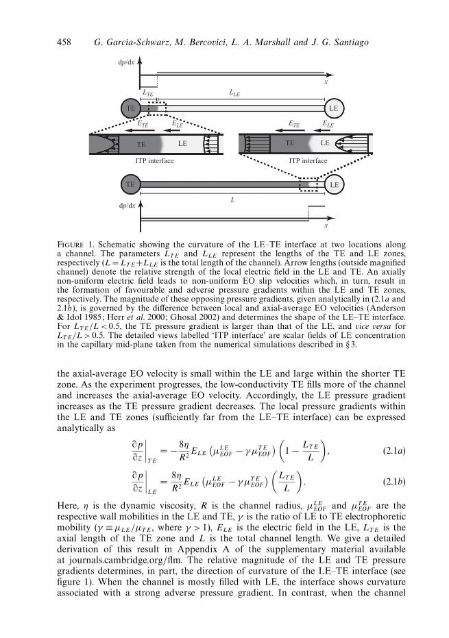
often modelled using a simple slip velocity condition known as the Helmholtz–Smoluchowski equation (Probstein 1994). This boundary condition provides a linearrelationship between EO slip and local applied electric field and can be applied to flowswith non-uniform conductivities (Santiago 2001). In ITP, a current applied throughaxial conductivity gradients creates electric field gradients that lead to analyte focusing.The electric field is uniform within both the LE and the TE, and its value in each zonecan be related through the ITP condition, µLEELE = µT EET E (Everaerts, Beckers &Verheggen 1976). Axial variation of the electric field also causes non-uniform EO slipvelocities, depicted in figure 1, which in turn generate internal pressure gradients. Farfrom the LE–TE interface, local pressure gradients are uniform and proportional tothe di!erence between local and axial-average EO velocities (Anderson & Idol 1985;Herr et al. 2000; Ghosal 2002). An adverse pressure gradient (relative to bulk flow)forms in the TE where the EO slip is typically higher than the axial-average EOF,and a favourable pressure gradient forms in the LE where the EO slip is typicallylower than the axial-average EOF.

Figure 1 describes some of the main features of ITP boundaries dispersed by non-uniform EOF. Throughout this paper, we will assume negative EO mobility (typical forglass or silica for approximately pH 4 and above, see Kirby & Hasselbrink 2004) andanionic ITP, but the concepts are easily extended to cover cationic ITP and/or positivewall charge. Near the beginning of a typical ITP experiment, the high-conductivityLE fills most of the channel so that the axial-average EOF is dominated by the EOslip in the LE zone. In this case, the mismatch between the local EO slip velocity and


TE

ETE ETE

LTE

x

LLE

ELE ELE

TE LETE LE

ITP interface ITP interface

TE

dp/dx

dp/dx

L

x

LE

LE

Figure 1. Schematic showing the curvature of the LE–TE interface at two locations alonga channel. The parameters LT E and LLE represent the lengths of the TE and LE zones,respectively (L =LT E+LLE is the total length of the channel). Arrow lengths (outside magnifiedchannel) denote the relative strength of the local electric field in the LE and TE. An axiallynon-uniform electric field leads to non-uniform EO slip velocities which, in turn, result inthe formation of favourable and adverse pressure gradients within the LE and TE zones,respectively. The magnitude of these opposing pressure gradients, given analytically in (2.1a and2.1b), is governed by the di!erence between local and axial-average EO velocities (Anderson& Idol 1985; Herr et al. 2000; Ghosal 2002) and determines the shape of the LE–TE interface.For LT E/L < 0.5, the TE pressure gradient is larger than that of the LE, and vice versa forLT E/L > 0.5. The detailed views labelled ‘ITP interface’ are scalar fields of LE concentrationin the capillary mid-plane taken from the numerical simulations described in § 3.

the axial-average EO velocity is small within the LE and large within the shorter TEzone. As the experiment progresses, the low-conductivity TE fills more of the channeland increases the axial-average EO velocity. Accordingly, the LE pressure gradientincreases as the TE pressure gradient decreases. The local pressure gradients withinthe LE and TE zones (su"ciently far from the LE–TE interface) can be expressedanalytically as

!p

!z

!!!!T E

= " 8!

R2ELE

"µLE

EOF " "µT EEOF

# $1 " LT E

L

%, (2.1a)

!p

!z

!!!!LE

=8!

R2ELE

"µLE

EOF " "µT EEOF

# $LT E

L

%. (2.1b)

Here, ! is the dynamic viscosity, R is the channel radius, µLEEOF and µT E

EOF are therespective wall mobilities in the LE and TE, " is the ratio of LE to TE electrophoreticmobility (" # µLE/µT E , where " > 1), ELE is the electric field in the LE, LT E is theaxial length of the TE zone and L is the total channel length. We give a detailedderivation of this result in Appendix A of the supplementary material availableat journals.cambridge.org/flm. The relative magnitude of the LE and TE pressuregradients determines, in part, the direction of curvature of the LE–TE interface (seefigure 1). When the channel is mostly filled with LE, the interface shows curvatureassociated with a strong adverse pressure gradient. In contrast, when the channel


is mostly filled with TE, the interface shows curvature associated with a stronglyfavourable pressure gradient. The detailed views showing ‘ITP interface’ scalar fieldsin figure 1 are results from numerical simulations presented in § 3.

EOF also a!ects the velocity of ITP zones. The axial-average EOF velocity (UEOF )acts against anion electromigration and thus results in a reduced zone velocity,Uzone . This adjusted zone velocity depends on values of EO mobility in the TE andLE as well as the axial position of the LE–TE interface. The adjusted velocity,Uzone = UITP + UEOF , can be expressed as

Uzone = µLEELE +

&$LT E

L

%µT E

EOFET E +

$1 " LT E

L

%µLE

EOFELE

'. (2.2)

Here UITP # µLEELE is the ITP velocity in the absence of EOF, µLE is the LEelectrophoretic mobility and ET E is the electric field in the TE. The interplay ofelectrophoresis and EOF can have drastic e!ects on ITP. For example, the samplezone will not enter the channel from the TE reservoir if the EO mobility in the LEis greater than the LE electrophoretic mobility (µLE

EOF >µLE). When instead the EOmobility in the TE is greater than the LE electrophoretic mobility (µT E

EOF >µLE), thesample zone eventually becomes stationary within the channel where the bulk flowvelocity exactly counterbalances the ITP velocity (UEOF = " UITP ). Under the lattercondition, the sample zone can also enter the channel from the LE reservoir (for thecase where the channel is initially filled entirely with TE).

3. Numerical simulations of dispersion in ITP3.1. Governing equations and boundary conditions

In this section we present the governing equations for our numerical model of ITP. Weassume that all species are dilute and monovalent. We define the total concentration,ci , of a monovalent species i as

ci = ci,0 + ci,±1, (3.1)

where ci,0 is the concentration of its neutral form and ci,±1 is the concentration of itsionized form (with valence of +1 or "1). We define the e!ective mobility of the ithspecies as

µi =

$ci,±1

ci

%µi,±1, (3.2)

where µi,±1 is the corresponding fully ionized mobility. With these conventions andsimplifications, the general convective-di!usion equation governing transport of theLE, TE, counter-ion and analyte through electromigration, di!usion and convectionis

!ci

!t+ ! · [uci + ziµi Eci " Di!ci] = 0 for i = LE, TE, CI, A. (3.3)

Here ci is the total concentration of the ith species, u is the fluid velocity field, zi is thevalence of the ith species, µi is the e!ective electrophoretic mobility of the ith species,Di is the di!usivity of the ith species and E is the electric field. In general E = " !#,where # is the electric potential. The subscripts CI and A refer respectively to thecounter-ion (here a cation) and the focused analyte ion. We use the Nernst–Einsteinequation to relate ion di!usivity to electrophoretic mobility, Di =µi,±1RµT/F , whereRµ is the gas constant, T is the temperature in kelvin and F is Faraday’s constant.


The fluid velocity and pressure are governed by the low-Reynolds-number Stokesequations with an electric body force,

!p = !$2u + [$! · E] E, (3.4)

! · u = 0. (3.5)

Here p is the pressure and $ is the electrolyte permittivity. The final term in themomentum equations represents the electric body force, which accounts for a forceexerted on the fluid by regions of net free charge moving under the influence of anelectric field. In our domain of interest, this net charge resides in the bulk liquid(outside the electric double layer) and is associated with the coupling of electric fieldand conductivity gradients (see Lin et al. 2004 for further discussion). We assumeconstant permittivity and extract $ from the divergence operator.

The electric potential is governed by the conservation of charge,

!%e

!t+ ! · j = 0, (3.6)

where

j = F

(E

)

i

ziµi,zici,zi

+ u)

i

zici,zi"

)

i

ziDi!ci,zi

*. (3.7)

Here %e is the free charge density and j is the current density, which includesconductive, convective and di!usive components.

As mentioned above, conductivity gradients in ITP lead to distributions of netcharge in the bulk liquid. However, as discussed by Saville & Palusinski (1986), inITP the characteristic length scale of the conductivity interface is typically much largerthan the electric length scale associated with regions of significant net charge (i.e.much larger than the Debye length). We can therefore invoke the electroneutralityapproximation and neglect the unsteady and convective terms in (3.6). Under theelectroneutrality approximation, we still account for forces associated with even asmall amount of net charge by retaining the body force term in the momentumequation. We refer the reader to Appendix B in the supplementary material for amore detailed derivation of the electroneutrality approximation using perturbationanalysis. We express the electroneutrality approximation as

)

i

zi

$µi

µi,zi

%ci % 0. (3.8)

In our formulation, we use (3.8) in place of the counter-ion species transport equation(the convective-di!usion equation for cCI ) to close the system of governing equations.

This formulation constitutes a total of eight equations for eight unknowns (cLE ,cT E , cCI , cA, u, v, p and #). The final form of the governing equations is

!ci

!t+ ! · [uci + ziµi Eci " Di!ci] = 0 for i = LE, TE, A, (3.9)

)

i

zi

$µi

µi,zi

%ci % 0, (3.10)

!p = !$2u + $ [! · E] E, (3.11)

! · u = 0, (3.12)


! ·(

E)

i

ziµici ")

i

ziDi

$µi,zi

µi

%!ci

*= 0. (3.13)

We performed all numerical simulations with the commercial package COMSOLMultiphyscis (version 3.5, COMSOL AB, Stockholm, Sweden) using the Nernst–Planck and incompressible Navier–Stokes modules. We reduced computational cost byaxially truncating the channel domain and transforming the flow boundary conditionsto a frame of reference moving with the sample zone. The velocity of this frame ofreference, Uzone , is given in (2.2). The transformed boundary conditions for the species,velocity, pressure and electric potential were the same as those given by Schonfeldet al. (2009) and are reproduced in Appendix C of the supplementary material.

We discretized the domain using rectangular mesh elements with a uniform griddensity in the radial dimension. We used non-uniform grid spacing in the axialdimension with high resolution in the interface region (&0.5 µm) and much lowerresolution within the LE and TE zones (&5 µm on average), which remain at steadystate. We used a total of 16 000 cells throughout the domain. Additionally, weperformed tests to assess the grid sensitivity at this resolution and established gridindependence. More details regarding domain discretization are provided in AppendixC of the supplementary material.

3.2. Simulation results

We use our numerical simulations to investigate the impact of analyte mobility andnon-uniform EOF on sample distributions in ITP. A table with parameter valuesused in our simulations is provided in Appendix D of the supplementary material.Unless otherwise noted, for this part of our study the simulation parameters reflectthe LE and TE chemistry of the validation experiments presented in § 5. We non-dimensionalize the applied current density, j , with a characteristic current densityjR . We define jR as the current density in a non-dispersed ITP process where theLE–TE interface width (&) is equal to the channel radius (R). The width of the LE–TEinterface is given by the one-dimensional theory of MacInnes & Longsworth (1932)as

& # 4RµT

FUITP

µLEµT E

µLE " µT E

. (3.14)

The derivation of this result neglects the di!usive component of current density,which is typically small compared to the electromigration component. We thereforeexpress the current density as j = 'LEELE , where 'LE = F (zLEµLEcLE + zCIµCI cCI ) isthe LE conductivity. We rearrange (3.14), letting & = R, to solve for the characteristiccurrent density

jR # 4RµT

F

$µT E

µLE " µT E

%'LE

R. (3.15)

For the simple case of ITP without EOF, an analyte focused at the LE–TE interfacehas a finite distribution width determined solely by the balance between di!usionand electromigration. Even in this case, the penetration length of the focused analyteinto each of its bracketing zones depends strongly on its electrophoretic mobilityrelative to the LE and TE. For example, an analyte with mobility very near the TEmobility will experience a strong restoring force upon di!using into the LE zone buta weak restoring force upon di!using into the TE zone. This results in greater samplepenetration into the TE. We demonstrate this e!ect in figure 2 using area-averagedanalyte distributions predicted by simulations of non-dispersed ITP with relatively


1 2 3 4 5

1 1

00 1 2 3

x/R x/R4 5

CA

/Cm

ax

C

C

B

A

A

A. exp(x/!TE)B. exp((x–")2/s2)C. exp(x/!LE)

A. exp(x/!TE)B. exp((x–")2/s2)C. exp(x/!LE)

B

EE

(a) (b)µA /µ– = 0.76 LTE /L = 0.07 µA /µ– = 2 LTE /L = 0.93

CTECTE

CLECLE

III III

IIII

II

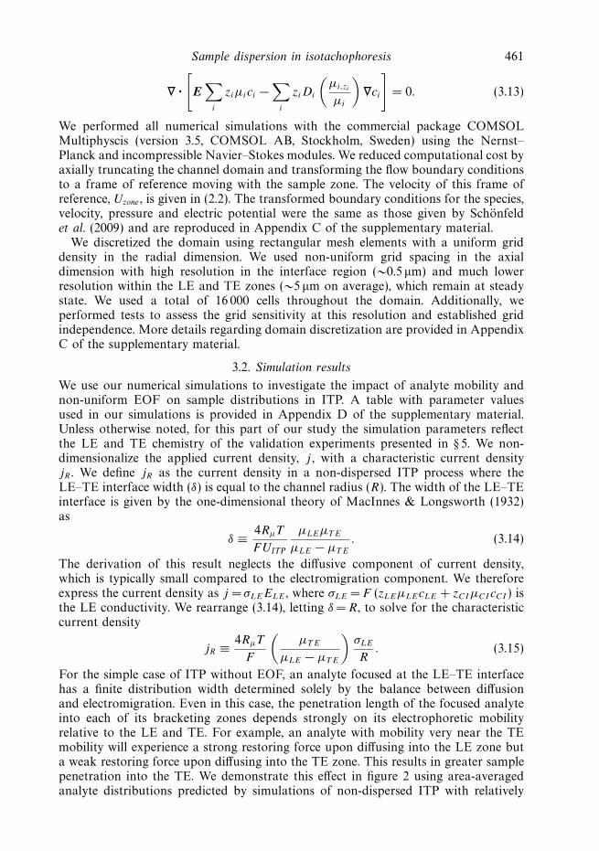
Figure 2. Schematic showing the construction of the analytical model and comparing this toarea-averaged sample distributions from dispersed and non-dispersed numerical simulations.We fix current density at j/jR = 3.13 and consider two conditions: µA/µ = 0.76, LT E/L = 0.07(a) and µA/µ = 2, LT E/L = 0.93 (b). Here the constant µ (defined in § 4.1) is the value ofanalyte mobility at which the sample distribution is symmetric under non-dispersed conditions(µEOF = 0) . We assume that EO mobility is axially uniform (µEOF = µT E

EOF = µLEEOF ) and consider

the case where µEOF/µLE = 0.22 for simulations that include dispersion. Two-dimensionalconcentration profiles of the dispersed sample are shown in row II along with superimposedlines tangent to combined electromigration and convective mass flux components. Thearea-averaged distributions corresponding to this dispersed case and to the non-dispersedsimulations are shown in row III as red (solid) and blue (dot) curves, respectively. In bothcases dispersion a!ects the already strongly tailing portions of the distributions. The analyticalmodel prediction, which is also shown (dashed curve), is composed of two exponential tailsmatched to a central Gaussian. The matching points (xi , defined in § 4.1) are shown withvertical dashed lines in row III. These vertical lines extend to row I, where we show thearea-average LE and TE species concentrations along with the area-average electric field fromsimulations including dispersion. The location of the matching points reveals that the tails ofthe distribution (regions A and C) correspond to the regions of uniform electric field, whilethe central Gaussian (region B) corresponds to a region of strong electric field gradient.

low- and high-mobility analytes (figures 2a and 2b, respectively). We divide the sampledistribution into three parts, corresponding to the two ‘tails’ of the sample distribution(regions A and C) and to its central peak (region B). Under non-dispersed conditions,a low analyte mobility results in strong sample penetration into the TE zone (regionA), while a high analyte mobility results in strong penetration into the LE zone(region C).

Figure 2 also shows area-averaged sample distributions from simulations with non-zero EO mobility (solid curves, bottom row). The corresponding area-averaged axialelectric field is shown in the top row of figure 2. For figures 2(a) and 2(b), whichcorrespond to relatively low- and high-mobility analytes, respectively, we choosethe axial interface position corresponding to a dominant pressure gradient in thezone of greater sample penetration. The resulting strong parabolic flow broadensthe distribution tails in these respective zones while leaving the other tail nearlyunchanged. We note that the tails of the sample distribution (regions A and


C) occupy regions of approximately uniform electric field while the peak of thedistribution (region B) lies within a strong electric field gradient. The regions ofuniform electric field correspond to uniform parabolic flow profiles. This suggeststhat analyte distribution tails primarily experience axially uniform dispersive flow.

The middle row of figure 2 depicts the centreline sample concentration field of thedispersed analytes. Lines tangent to the vector sum of electromigration and advectivevelocities are also depicted. These images show the interface position-dependentcurvature of the sample zone discussed in § 2 (see figure 1). In the near-TE-reservoirposition (figure 2a) the transverse curvature resembles the favourable parabolic flowin the TE, while in the near-LE-reservoir position (figure 2b) the curvature insteadresembles the adverse parabolic flow in the LE. The latter finding regarding pressuregradients is consistent with the numerics of Schonfeld et al. (2009), and the analytepeak shape of figure 2(b) is consistent with their qualitative visualizations. In contrastto that work, here we also model the strong e!ect of analyte mobility relative to theTE and LE, which results in e!ects of analyte tailing and enhanced dispersion, asdescribed above.

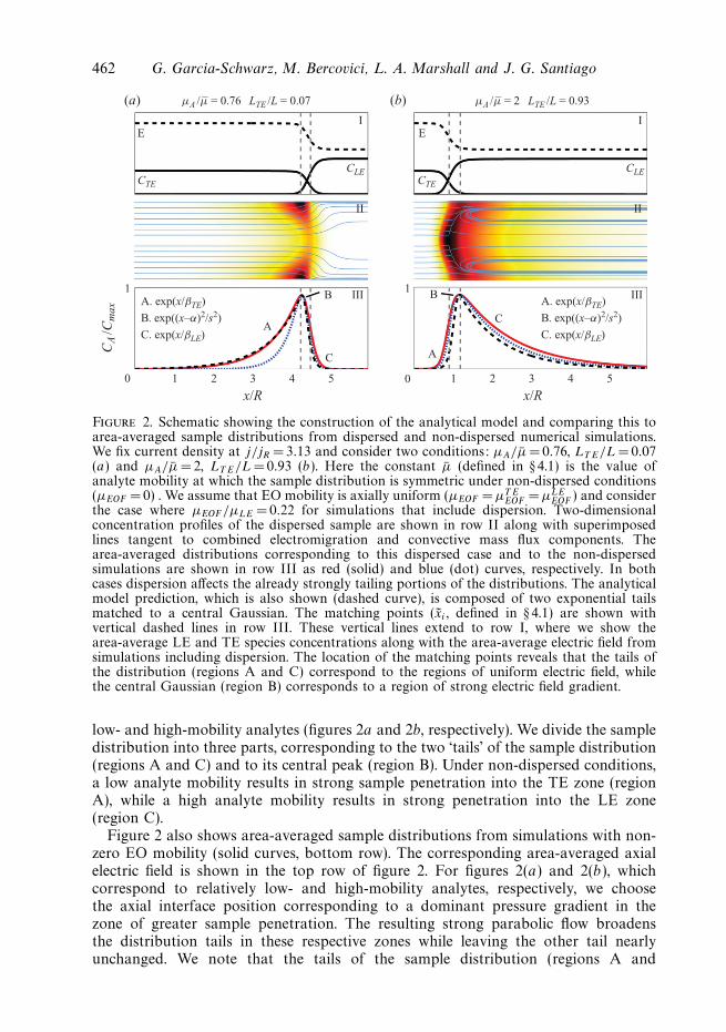
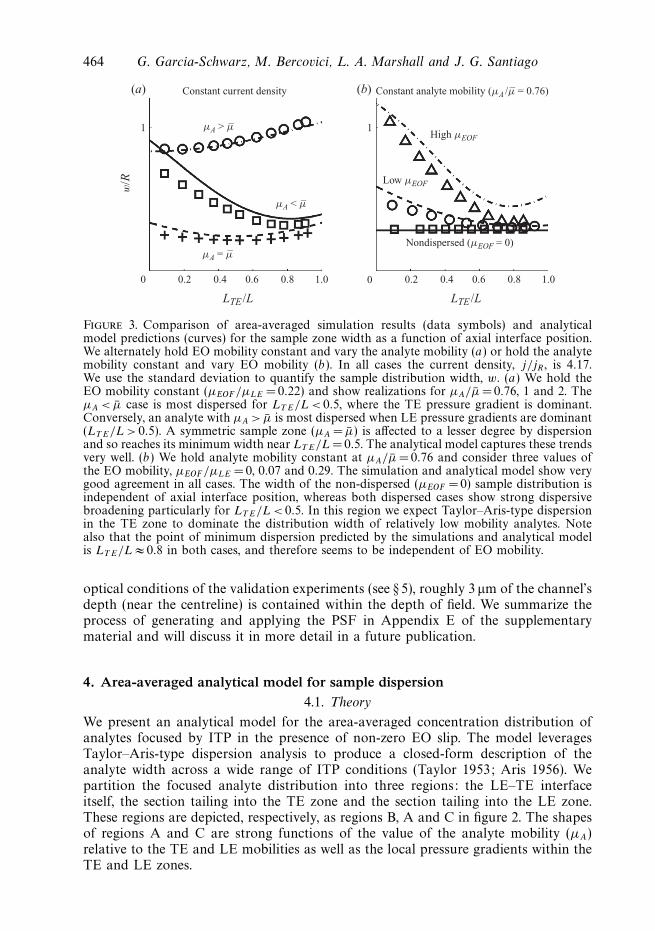
In figure 3 we summarize the dependence of analyte distribution widths (w) onanalyte mobility, axial interface position and EO mobility. We use the axial standarddeviation of the area-averaged analyte concentration to quantify the distribution widthand also as an inverse measure of sensitivity. We plot curves of the analyte distributionwidth against axial interface position for three analyte mobilities in figure 3(a) andthree EO mobilities in figure 3(b). The analyte mobility is compared to a characteristicmobility scale, µ, which results in approximately symmetric analyte profiles and isdescribed in detail in § 4. Figure 3(a) shows that, in general, dispersion is greatest atthe two extremes of the channel, with a minimum width typically achieved withinroughly the middle portion of the channel. Analytes with relatively near-TE or near-LE mobility exhibit strong dispersion when near the TE or LE reservoir, respectively.In each case, the most dispersed region corresponds to axial interface positions wherethe dominant pressure gradient coincides with the zone of greater sample penetration.The intermediate case (where µA = µ) has a symmetric distribution with a minimumin dispersion near the channel’s axial centre, LT E/L = 0.5. By comparison with theother cases where µA/µ is smaller or greater than 1, we note that the point ofminimum dispersion is strongly dependent on analyte mobility. In figure 3(b) weconsider a fixed analyte mobility (µA/µ = 0.76) and vary dimensionless EOF mobility(µEOF/µLE) for values commonly observed in glass channels at this pH. For the caseof zero dispersion (µEOF = 0), the analyte distribution width is independent of axialinterface position. As EO mobility increases, analyte dispersion increases primarily inthe near-TE-reservoir region and remains nearly unchanged elsewhere. Note that forthis low-mobility analyte, the width of the distribution is approximately insensitiveto the magnitude of the pressure gradient in the LE, as all of the curves shown infigure 3(b) approach the same value in the LT E/L > 0.5 region. Additionally, both ofthe dispersed curves shown in figure 3(b) (and others we examined) have a point ofminimum dispersion around LT E/L =0.8. This suggests that the point of minimumdispersion is at most weakly dependent on EO mobility.

To aid in later comparisons with experimental data, we approximated the di!ractivee!ects of microscope imaging on simulation data. In figures 6 and 7, which arediscussed at length in § 5, we convolve our numerical data with a three-dimensionaloptical point spread function (PSF) that accounts for di!raction introduced bythe microscope objective. In this three-dimensional convolution, we account for thevarying values of magnification at each plane relative to the focal plane. Under the


0.2 0.4

LTE /L LTE /L

0.6 0.8 1.0

11

(a) (b)

0

w/R

0 0.2

Nondispersed (µEOF = 0)

Constant analyte mobility (µA /µ– = 0.76)Constant current density

High µEOF

Low µEOF

0.4 0.6 0.8 1.0

µA = µ–

µA < µ–

µA > µ–

Figure 3. Comparison of area-averaged simulation results (data symbols) and analyticalmodel predictions (curves) for the sample zone width as a function of axial interface position.We alternately hold EO mobility constant and vary the analyte mobility (a) or hold the analytemobility constant and vary EO mobility (b). In all cases the current density, j/jR , is 4.17.We use the standard deviation to quantify the sample distribution width, w. (a) We hold theEO mobility constant (µEOF/µLE = 0.22) and show realizations for µA/µ = 0.76, 1 and 2. TheµA < µ case is most dispersed for LT E/L < 0.5, where the TE pressure gradient is dominant.Conversely, an analyte with µA > µ is most dispersed when LE pressure gradients are dominant(LT E/L > 0.5). A symmetric sample zone (µA = µ) is a!ected to a lesser degree by dispersionand so reaches its minimum width near LT E/L = 0.5. The analytical model captures these trendsvery well. (b) We hold analyte mobility constant at µA/µ =0.76 and consider three values ofthe EO mobility, µEOF/µLE = 0, 0.07 and 0.29. The simulation and analytical model show verygood agreement in all cases. The width of the non-dispersed (µEOF = 0) sample distribution isindependent of axial interface position, whereas both dispersed cases show strong dispersivebroadening particularly for LT E/L < 0.5. In this region we expect Taylor–Aris-type dispersionin the TE zone to dominate the distribution width of relatively low mobility analytes. Notealso that the point of minimum dispersion predicted by the simulations and analytical modelis LT E/L % 0.8 in both cases, and therefore seems to be independent of EO mobility.

optical conditions of the validation experiments (see § 5), roughly 3 µm of the channel’sdepth (near the centreline) is contained within the depth of field. We summarize theprocess of generating and applying the PSF in Appendix E of the supplementarymaterial and will discuss it in more detail in a future publication.

4. Area-averaged analytical model for sample dispersion4.1. Theory

We present an analytical model for the area-averaged concentration distribution ofanalytes focused by ITP in the presence of non-zero EO slip. The model leveragesTaylor–Aris-type dispersion analysis to produce a closed-form description of theanalyte width across a wide range of ITP conditions (Taylor 1953; Aris 1956). Wepartition the focused analyte distribution into three regions: the LE–TE interfaceitself, the section tailing into the TE zone and the section tailing into the LE zone.These regions are depicted, respectively, as regions B, A and C in figure 2. The shapesof regions A and C are strong functions of the value of the analyte mobility (µA)relative to the TE and LE mobilities as well as the local pressure gradients within theTE and LE zones.


The unsteady time scale is the time for the ITP zone to move a significant fractionof the channel length, L/ |Uzone |. This value is on the order of 100 s for the regimesof interest here and is thus significantly larger than the time scales associated withdi!usion and electromigration, both on the order of 0.1 s (see below for a discussionof relevant dispersion time scales). We therefore assume quasi-steady-state dispersionthroughout the channel length. We approximate focusing dynamics in A and C byassuming that these regions have a uniform axial pressure gradient and electricfield. In region B, we approximate the electric field as a linear function of the axialdimension, x. In constructing this approximate model, we assume that all variablesare uniform in the radial dimension, r . For each of the three regions, the steady-stateflux conservation equation for the area-averaged analyte concentration (Bharadwajet al. 2008) in a frame of reference moving with the ITP zones (Uzone , see (2.2)) is

d

dx

&$µAEcA + UEOFcA " De!

dcA

dx

%" UzonecA

'= 0. (4.1)

Here E is the axial electric field, cA is the (area-averaged) analyte concentration,UEOF is the axial-average EOF velocity and De! is the analyte e!ective Taylordispersion di!usivity (Taylor 1953; Aris 1956; Bharadwaj et al. 2008). We cangenerally separate and integrate (4.1) for the analyte concentration assuming zeroconcentration su"ciently far from the LE–TE interface to find

cA = Ki exp

$+µAE " UITP

De!dx

%, (4.2)

where Ki is a constant of integration. As mentioned above, we approximate theelectric field as uniform su"ciently far from the LE–TE interface and linear acrossthis boundary. In regions A and C, the e!ective di!usivity is determined by thepressure gradient in the TE and LE, respectively:

De! ,i = DA

(1 +

1

48

$RUi

DA

%2*, (4.3)

where

U i # µiEOFEi "

&$LT E

L

%µT E

EOFET E +

$1 " LT E

L

%µLE

EOFELE

'. (4.4)

The subscript i denotes the TE or LE regions (respectively A and C in figure 2). U i

is the magnitude of the dispersive (parabolic) flow component, whose area average isequal to the di!erence between the local and axial-average EO velocities.

We can therefore express (4.2) separately for regions A, B and C as follows:

cT EA = KT E exp

&$µAET E " UITP

De! ,T E

%x

', (4.5a)

cINTA = KINT exp

&1

DA

+ $µA

$(E

a&x + E

%" UITP

%dx

', (4.5b)

cLEA = KLE exp

&$µAELE " UITP

De! ,LE

%x

'. (4.5c)

Here cT EA , cINT

A and cLEA are the analyte concentrations in the TE, interface

and LE regions, respectively. KT E , KINT and KLE are the correspondingconstants of integration. E is the arithmetic average of the (axial) electric fields,


E # (ET E + ELE) /2, and the di!erence in the electric field between the LE and TEzones is denoted as (E # ELE " ET E . We hypothesize that the contribution of theinterface region (region B) to the distribution width is negligible when compared toits dispersed tails (regions A and C). We further assume that the interface regionis well-modelled without accounting for dispersion. In (4.5b), we therefore use theanalyte di!usitvity, DA, in place of De! . We also write the electric field in this region interms of the di!usion-limited width of the interface, a&. The dimensionless constanta is the prefactor introduced to scale the LE–TE interface width as given by thesimple relation in (3.14). In our model, this prefactor determines the slope of theelectric field at the LE–TE interface, neglecting dispersion. We determined the valueof a by analysing the electric field gradient of area-averaged numerical simulationsof ITP neglecting dispersion, similar to those performed by Khurana & Santiago(2008). For a fairly wide range of applied current densities, we find that a prefactorvalue of a % 1.58 best describes the slope of the electric field at its point of inflection(located within region B). We refer the reader to Appendix F for further details onthe determination of a.

Lastly, we determine analytically the coe"cients Ki of each region by imposing threematching conditions to produce a composite, smooth, area-averaged concentrationdistribution: (i) function values must be equal at both matching points, xi (i.e. theA–B and B–C interfaces), (ii) function derivatives must be equal at both matchingpoints (to guarantee smoothness of the distribution) and (iii) the integral of thecomposite solution must reflect the total amount of accumulated sample. We notethat continuity of the electric field is not ensured under these conditions.

By imposing these conditions and solving (4.5a)–(4.5c) we arrive at the followingcomposite solution for the one-dimensional (area-averaged) sample distribution alongthe axial dimension, x:

cA (x) = K

,--------.

--------/

exp

&)

*T E

+s2

(2*T E)2

'exp

&x

*T E

', x < xT E

exp

&" (x + ))2

s2

', xT E < x < xLE,

exp

&)

*LE

+s2

(2*LE)2

'exp

&x

*LE

', x > xLE

(4.6)

where

xi =s2

2*i

" ), (4.7)

*LE

&=

1

4

µA(µLE " µT E)

µT E(µA " µLE)

De! ,LE

DA

, (4.8)

*T E

&=

1

4

µA(µLE " µT E)

µLE(µA " µT E)

De! ,T E

DA

, (4.9)

s

&=

0a

2, (4.10)

)

&= a

&1

2" µLE

µA

$µA " µT E

µLE " µT E

%'. (4.11)


Here *i and s naturally arise as characteristic length scales for the regions of uniformand linear electric field, respectively. ) is an axial displacement (relative to the centreof the LE–TE interface) of the peak value of the central Gaussian portion of the curve(see region B in figure 2). The constant K normalizes the distribution so that its axialintegral reflects the total accumulated amount of sample. We note that the matchingpoints, xi , are entirely determined by the continuity and smoothness conditions above.

An important contribution of this model is that it accounts for analyte properties(e.g. analyte mobility) in determining the distribution width. To establish a basis ofcomparison between relatively low and relatively high values of analyte mobility, wecan derive the analyte mobility that results in an approximately symmetric distribution,µ. A symmetric distribution results when the analyte focuses in the central portionof the electric field gradient (x = 0 in figure 2) such that the tails in regions A and Cdecay over the same length scale (i.e. when *T E = "*LE). In our analytical model, thelocation of the analyte peak is governed by the parameter ), which shifts the positionof the central Gaussian of region B. These conditions are satisfied by letting ) =0(or, equivalently, by letting *T E = "*LE and De! ,i = DA) and solving for the resultinganalyte mobility. Thus, the analyte mobility resulting in a symmetric distribution is

µ =µLEµT E

12 (µLE + µT E)

. (4.12)

For µA < µ we expect that the sample will have a longer penetration length in theTE, while for µA > µ we expect a longer penetration length in the LE.

In addition to µA/µ, we also use (µA " µT E) / (µLE " µT E) as a non-dimensionalparameter describing analyte mobility. The latter parameter appears in (4.11) andvaries from a minimum value of zero (where µA = µT E) to a maximum value of 1(where µA = µLE). Analytes with e!ective mobility outside this range do not focus.We use this normalization parameter for the contour maps in figure 4 and elsewhereuse µ as a non-dimensional parameter describing analyte tailing.

Before continuing, we note that the main assumption underlying Taylor–Arisdispersion analysis is that the time scale of radial di!usion, tr , should be smallcompared to the time scale(s) of axial dispersion, tdisp . The radial di!usion time istr = R2/DA and, under typical conditions, has a value on the order of 0.1 s. Thereare several possible time scales for the dispersion process. These include the unsteadytime scale, L/ |Uzone | (discussed above), and the characteristic focusing time associatedwith analyte axial electromigration, !/ |UA| (here UA = µAEi " UITP is the relativevelocity of the analyte with respect to the moving LE–TE interface and ! is thelength of the analyte zone). However, these time scales do not account for the directdependence of the dispersive process on EO mobility. Thus, perhaps the most relevantis an axial dispersion time scale governed by the magnitude of the non-uniform flowcomponent of the velocity and the characteristic length scale of the analyte zone,tdisp = !/ |µEOF(E|. Here, we find the velocity magnitude by evaluating (4.4) for thehighest value of U i (cf., figure 1). The length of the analyte zone, !, scales as thetailing dimension *i . For a symmetric analyte, µA % µ, tailing is minimal and tdisp is onthe order of 0.1 s. For cases with significant tailing (e.g. µA < µ), ! increases and thevalue of tdisp can be on the order of 1 s. While the condition tr ' tdisp does not alwayshold strictly, we believe that the Taylor–Aris analysis is a useful approximation formodelling dispersion in ITP under a wide variety of conditions. As we will show, theTaylor–Aris approximation leads to very good agreement between our area-averagedmodel, numerical simulations and experiments.


0.1

0.2

0.3

0.4

0.5

0.6

0.7

0.8

0.9

(a) (b)j/jR = 0.52 j/jR = 4.69

0.1

0.2

0.3

0.4

0.5

0.6

0.7

0.8

0.9

0.2 0.4 0.6 0.8

14

8

7

6

5

4

3

2

1

12

10

8

6

4

2

0.2 0.4 0.6 0.8

µA = µ– µA = µ–

LTE/L LTE/L

w/Rw/R(µ

A –

µTE

)/(µ

LE –

µTE

)

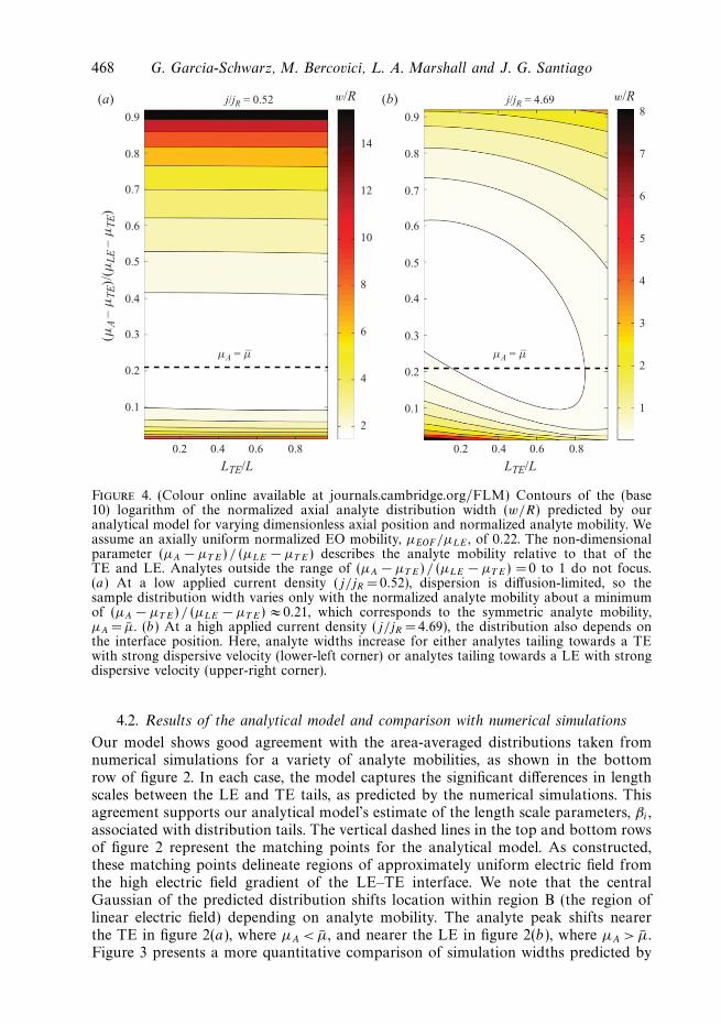
Figure 4. (Colour online available at journals.cambridge.org/FLM) Contours of the (base10) logarithm of the normalized axial analyte distribution width (w/R) predicted by ouranalytical model for varying dimensionless axial position and normalized analyte mobility. Weassume an axially uniform normalized EO mobility, µEOF/µLE , of 0.22. The non-dimensionalparameter (µA " µT E) / (µLE " µT E) describes the analyte mobility relative to that of theTE and LE. Analytes outside the range of (µA " µT E) / (µLE " µT E) = 0 to 1 do not focus.(a) At a low applied current density (j/jR = 0.52), dispersion is di!usion-limited, so thesample distribution width varies only with the normalized analyte mobility about a minimumof (µA " µT E) / (µLE " µT E) % 0.21, which corresponds to the symmetric analyte mobility,µA = µ. (b) At a high applied current density (j/jR = 4.69), the distribution also depends onthe interface position. Here, analyte widths increase for either analytes tailing towards a TEwith strong dispersive velocity (lower-left corner) or analytes tailing towards a LE with strongdispersive velocity (upper-right corner).

4.2. Results of the analytical model and comparison with numerical simulations

Our model shows good agreement with the area-averaged distributions taken fromnumerical simulations for a variety of analyte mobilities, as shown in the bottomrow of figure 2. In each case, the model captures the significant di!erences in lengthscales between the LE and TE tails, as predicted by the numerical simulations. Thisagreement supports our analytical model’s estimate of the length scale parameters, *i ,associated with distribution tails. The vertical dashed lines in the top and bottom rowsof figure 2 represent the matching points for the analytical model. As constructed,these matching points delineate regions of approximately uniform electric field fromthe high electric field gradient of the LE–TE interface. We note that the centralGaussian of the predicted distribution shifts location within region B (the region oflinear electric field) depending on analyte mobility. The analyte peak shifts nearerthe TE in figure 2(a), where µA < µ, and nearer the LE in figure 2(b), where µA > µ.Figure 3 presents a more quantitative comparison of simulation widths predicted by


the analytical model and numerical simulations. Here analytical model predictionsof the sample distribution width show excellent agreement with simulations over awide range of conditions varying analyte mobility, applied current density and axialposition of the interface.

Having corroborated our analytical model with numerical simulations (cf., figures 2and 3), we now use this model to explore the dependence of the distribution width ona continuum of values of analyte mobility and axial interface position. Figure 4 showscontour maps of the analyte distribution width (scaled by the channel radius, R) asit varies with axial interface position and analyte mobility. Figures 4(a) and 4(b)respectively explore the cases of relatively low and high applied current densities,j/jR = 0.52 and 4.69 respectively. These values correspond to applied current densitiesof 0.80 and 7.16 A cm"2. For the lower applied current density, dispersion is di!usion-limited (dominated by the balance of di!usion and electrophoretic restoring fluxes)and therefore varies only with analyte mobility. Note that analyte mobility relativeto that of the TE and LE plays a key role in determining the sample zone width.For example, dispersion is negligible in figure 4(a) and yet w/R can vary significantlywith the non-dimensional mobility parameter. The distribution width is minimum forµA = µ, as per our derivation of (4.12), and significantly greater when µA approacheseither the mobility of the LE or TE. For example, for values of the scaled mobilityparameter of 0.2 and 0.9, w/R equals approximately 2 and 15, respectively. Athigher current densities, the e!ect of analyte mobility is compounded by the growingimportance of advective dispersion. Collectively, this results in a slanting of the w/Rcontours. Dispersion is greatest in two regions, namely the bottom-left and top-rightcorners of the plot. These regions correspond, respectively, to sample penetration inthe TE with dominant TE pressure gradient and sample penetration in the LE withdominant LE pressure gradient.

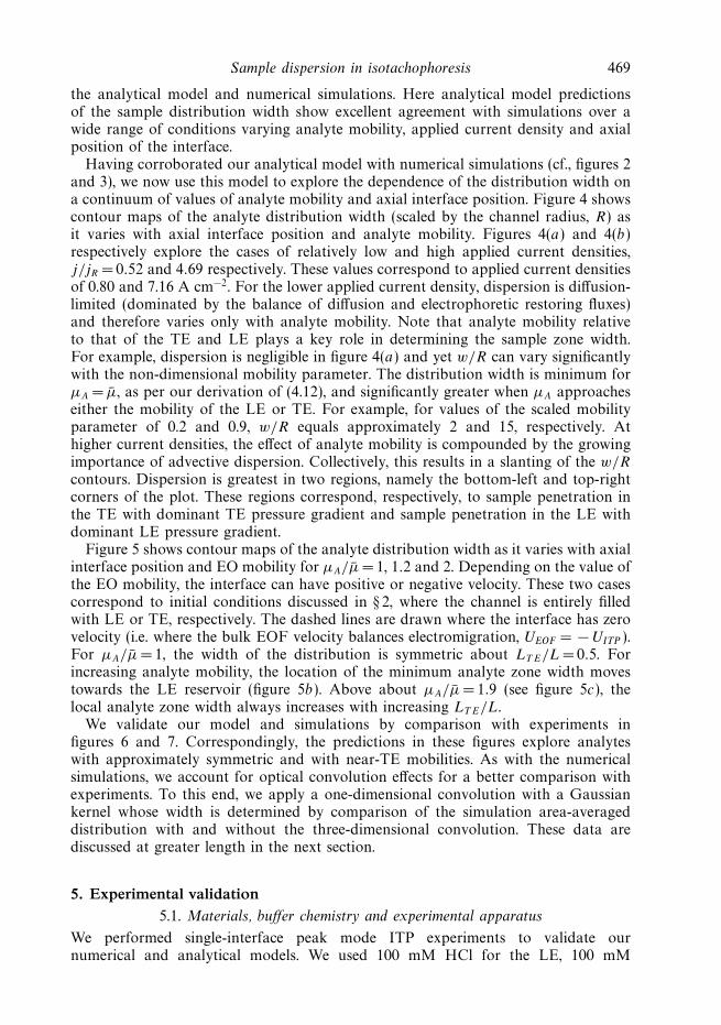
Figure 5 shows contour maps of the analyte distribution width as it varies with axialinterface position and EO mobility for µA/µ = 1, 1.2 and 2. Depending on the value ofthe EO mobility, the interface can have positive or negative velocity. These two casescorrespond to initial conditions discussed in § 2, where the channel is entirely filledwith LE or TE, respectively. The dashed lines are drawn where the interface has zerovelocity (i.e. where the bulk EOF velocity balances electromigration, UEOF = " UITP ).For µA/µ = 1, the width of the distribution is symmetric about LT E/L =0.5. Forincreasing analyte mobility, the location of the minimum analyte zone width movestowards the LE reservoir (figure 5b). Above about µA/µ = 1.9 (see figure 5c), thelocal analyte zone width always increases with increasing LT E/L.

We validate our model and simulations by comparison with experiments infigures 6 and 7. Correspondingly, the predictions in these figures explore analyteswith approximately symmetric and with near-TE mobilities. As with the numericalsimulations, we account for optical convolution e!ects for a better comparison withexperiments. To this end, we apply a one-dimensional convolution with a Gaussiankernel whose width is determined by comparison of the simulation area-averageddistribution with and without the three-dimensional convolution. These data arediscussed at greater length in the next section.

5. Experimental validation5.1. Materials, bu!er chemistry and experimental apparatus

We performed single-interface peak mode ITP experiments to validate ournumerical and analytical models. We used 100 mM HCl for the LE, 100 mM


0.20

0.2

0.4

0.6

0.8

1.0

0

0.2

0.4

0.6

0.8

0.5

1.0

1.5

2.0

0.5

1.0

1.5

2.0

2

3

4

51.0

0

0.2

0.4

0.6

0.8

1.0

0.4

Uzone > 0

Uzone < 0

Uzone = 0

0.6 0.8 0.2 0.4 0.6 0.8 0.2 0.4 0.6 0.8

µE

OF

/µLE

w/R w/R w/RµA /µ– = 1 µA /µ– = 1.2 µA /µ– = 2(a) (b) (c)

LTE /L LTE /L LTE /L

Figure 5. (Colour online) Contours of the (base 10) logarithm of the normalized axial analytedistribution width, w/R, predicted by our analytical model for varying dimensionless axialposition, LT E/L, and normalized EO mobility, µEOF/µLE . We hold current density constant(j/jR = 3.13) and, for simplicity, assume µEOF =µT E

EOF = µLEEOF . We show separate contour maps

for normalized analyte mobility values of µA/µ = 1, 1.2 and 2. The dashed line is drawnwhere the interface tends to zero velocity (i.e. where bulk EOF balances electromigration,UEOF = " UITP ). Solutions to the left of this line are for positive interface velocities, forexperiments where the channel is initially filled with LE. To the right, we show solutions forwhich interface velocity is negative, so that the channel is initially filled with TE and the zonetravels into the channel in the direction of EOF. For the latter case, µT E

EOFET E >UITP is anecessary condition for the interface to enter the channel from the LE reservoir. (a) For asymmetric sample distribution (µA/µ = 1), the contour map is symmetric about LT E/L = 0.5and the distribution width may reach a minimum at this point of symmetry. (b)–(c) As theanlayte mobility increases, the location of this minimum shifts towards lower values of LT E/L(e.g. near LT E/L = 0.3 when µA/µ =1.2) and vanishes altogether for µA/µ of about 1.9 orgreater.

2-(N-morpholino)ethanesulphonic acid (MES) for the TE and 200 mM Bis-Tris as thebackground bu!ering ion. We added 2 mM Ba(OH)2 to the TE in order to minimizezone broadening due to focusing of carbonic acid (see Khurana & Santiago 2009).We also prepared 1 µm stock solution of Alexa Fluor 488 (Invitrogen, Carlsbad,CA) and fluorescein (J.T. Baker, Phillipsburg, NJ), which we used to visualize asample zone focused in peak mode (anionic) ITP. All solutions were prepared inUltraPure DNase/RNase free distilled water (GIBCO Invitrogen, Carlsbad, CA). Thechemical properties for HCl, MES and Bis-Tris were obtained from the PeakMaster5.1 database (Jaros et al. 2004), which contains fully ionized mobility and pKa valuesdetermined by Hirokawa et al. (1983). We determined the fully ionized mobility ofAlexa Fluor 488 ("37 ( 10"9 m2 V"1 s"1) through on-chip capillary electrophoresis.For fluorescein, we chose the e!ective mobility to result in the best fit with simulationand model predictions. The resulting value ("18.9 ( 10"9 m2 V"1 s"1) is withinthe uncertainty bounds of values reported in the literature (Martin & Lindqvist1975; Mchedlov-Petrossyan, Kukhtik & Alekseeva 1994; Shakalisava et al. 2009) andaccepted models for ionic strength correction (Bahga, Bercovici & Santiago 2010).

We obtained images using an inverted epifluorescent microscope (IX70, Olympus,Hauppauge, NY) equipped with an LED lamp (LEDC1, Thor Labs, Newton, NJ) andU-MWIBA filter-cube from Olympus (460–490 nm excitation, 515 nm emission and


LTE/L = 0.2 LTE/L = 0.5 LTE/L = 0.8

40 µm

Experiment

Experiment

Inte

nsity

(A

U)

Model

Simulation

Simulation

x

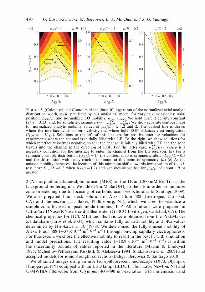
Figure 6. Comparison of our numerical simulations and analytical model with experimentsof focused Alexa Fluor 488 for j/jR = 3.13. We normalize all distributions to represent equalamounts of focused sample (i.e. all curve or area integrals normalized to unity). Simulationdistributions are adjusted to account for optical di!raction e!ects through convolution of thesimulation data with the theoretical three-dimensional PSF corresponding to the microscopeobjective. The analytical model inherently reflects a cross-sectional-area average, and so axialdistributions are adjusted by approximating the optical three-dimensional convolution as aone-dimensional convolution with a Gaussian. The simulations and model are in very goodagreement with experiments in both the two-dimensional and area-averaged distributions. Theconditions shown here are representative of both a typical ITP bu!er chemistry and valueof applied current density. For these experiments we used a 20 ( objective with 0.5 numericalaperture, 10 ms exposure time and a 40 µm inner diameter fused silica capillary.

505 nm cuto! dichroic). We used a 20 ( (NA = 0.5, WD = 2.1 mm) UPlanFl objectivefor Alexa Fluor 488 experiments and a 10 ( (NA = 0.4, WD = 3.1 mm) UPlanApoobjective for fluorescein experiments, both also from Olympus. We captured imagesusing a 12 bit, 1300(1030 pixel array CCD camera (Coolsnap-fx 16s, PrincetonInstruments, Trenton, NJ). We controlled the camera using Winview32 (PrincetonInstruments, Trenton, NJ) and processed the images with MATLAB (R2007b,Mathworks, Natick, MA). We triggered the camera at 10 Hz (Alexa Fluor 488experiments) and 5 Hz (fluorescein experiments) with an external signal generator(model 33220A, Agilent Technologies, Santa Clara, CA). We chose relatively lowexposure times of 10 ms (Alexa Fluor 488 experiments) and 20 ms (fluoresceinexperiments) to avoid smearing due to motion of the sample plug.

We performed all experiments in 40 µm inner diameter circular fused silicacapillaries (TSP040375, Polymicro Technologies, Phoenix, AZ). We removed thecapillary protective (and fluorescent) polyimide coating with the flame of a lighterto expose the fused silica. We immobilized the capillaries on a microscope slide withinstant adhesive (401, LOCTITE, Rocky Hill, CT). We fabricated reservoirs usingthreaded 1.5 ml tubes (64115, E&K Scientific, Santa Clara, CA) and used UV-curingoptical adhesive (no. 63, Norland Optical, Cranbury, NJ) to bond them to the surfaceat each end of the capillary. We covered the length of the capillary with a layer of


Experiment

Experiment

Exp.

–250

0.2

0.4

0.6

0.8

1.0

–20 –15

x/R–10 –5 0

Model

Simulation

Simulation

Sim.

LTE/L = 0.8

LTE/L = 0.2Inte

nsity

(A

U)

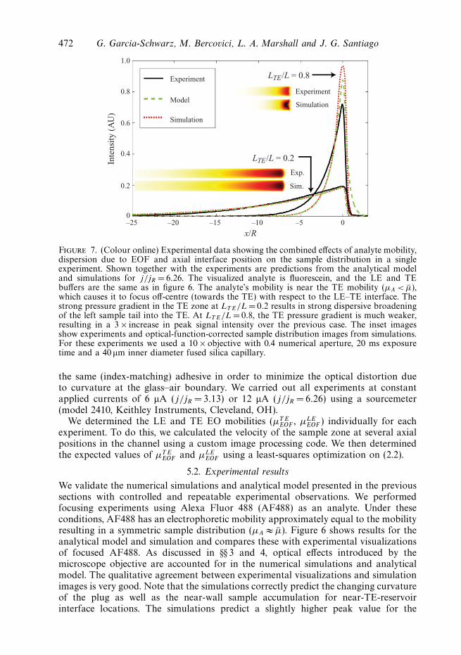
Figure 7. (Colour online) Experimental data showing the combined e!ects of analyte mobility,dispersion due to EOF and axial interface position on the sample distribution in a singleexperiment. Shown together with the experiments are predictions from the analytical modeland simulations for j/jR =6.26. The visualized analyte is fluorescein, and the LE and TEbu!ers are the same as in figure 6. The analyte’s mobility is near the TE mobility (µA < µ),which causes it to focus o!-centre (towards the TE) with respect to the LE–TE interface. Thestrong pressure gradient in the TE zone at LT E/L = 0.2 results in strong dispersive broadeningof the left sample tail into the TE. At LT E/L = 0.8, the TE pressure gradient is much weaker,resulting in a 3 ( increase in peak signal intensity over the previous case. The inset imagesshow experiments and optical-function-corrected sample distribution images from simulations.For these experiments we used a 10 ( objective with 0.4 numerical aperture, 20 ms exposuretime and a 40 µm inner diameter fused silica capillary.

the same (index-matching) adhesive in order to minimize the optical distortion dueto curvature at the glass–air boundary. We carried out all experiments at constantapplied currents of 6 µA (j/jR = 3.13) or 12 µA (j/jR =6.26) using a sourcemeter(model 2410, Keithley Instruments, Cleveland, OH).

We determined the LE and TE EO mobilities (µT EEOF , µLE

EOF ) individually for eachexperiment. To do this, we calculated the velocity of the sample zone at several axialpositions in the channel using a custom image processing code. We then determinedthe expected values of µT E

EOF and µLEEOF using a least-squares optimization on (2.2).

5.2. Experimental results

We validate the numerical simulations and analytical model presented in the previoussections with controlled and repeatable experimental observations. We performedfocusing experiments using Alexa Fluor 488 (AF488) as an analyte. Under theseconditions, AF488 has an electrophoretic mobility approximately equal to the mobilityresulting in a symmetric sample distribution (µA % µ). Figure 6 shows results for theanalytical model and simulation and compares these with experimental visualizationsof focused AF488. As discussed in §§ 3 and 4, optical e!ects introduced by themicroscope objective are accounted for in the numerical simulations and analyticalmodel. The qualitative agreement between experimental visualizations and simulationimages is very good. Note that the simulations correctly predict the changing curvatureof the plug as well as the near-wall sample accumulation for near-TE-reservoirinterface locations. The simulations predict a slightly higher peak value for the


area-averaged distribution than that observed in experiments but nonetheless capturethe axial dependence of distribution tailing. Sample distributions predicted by theanalytical model show excellent agreement with experiments.

In figure 7 we consider the more dramatic case of fluorescein as the focusedsample. Under these conditions, the value of the parameter µA/µ is approximately0.66, predicting strong tailing towards the TE. Shown are experimental data togetherwith predictions from both simulation and our analytical model. The TE and LEbu!ers are identical to those of figure 6 in order to highlight the dramatic e!ect ofanalyte mobility on distribution shape. The strong skew and tailing of the fluoresceindistribution makes the peak width sensitive to the pressure gradients in the TEzone. At LT E/L = 0.2, the measured standard deviation width is approximately sixtimes greater than the di!usion-limited (non-dispersed) minimum width due to stronganalyte tailing into the locally dispersive TE zone. For a near-LE-reservoir positionof LT E/L = 0.8, the TE pressure gradient is much weaker and dispersive broadeningdecreases significantly. For the latter case, the maximum analyte concentrationincreases by roughly a factor of 3 over the case where LT E/L = 0.2. The comparisonof fluorescein distribution between LT E/L = 0.2 and 0.8 shows the dramatic e!ectof analyte position on dispersion. This particular case of analyte dispersion dueto the combined e!ects of analyte mobility and EOF-associated dispersion showsthat detector placement can be of great importance in ITP assays with non-negligibleEOF. Once again, our model and simulations show good agreement with experimentaldata. The only significant di!erence is in the LT E/L = 0.2 case, where the simulationand model predict a significantly higher maximum concentration than found inexperiments. Nevertheless, the simulation and model capture the significant trendsincluding the shape of the sample distribution and the sharp increase in peakconcentration due to decreased dispersion in the TE. Once again, as in figure 6,the concentration distributions predicted by the analytical model show very goodagreement with experiments.

6. Summary and conclusionsAnalytes focused in peak mode ITP show strong penetration into the TE if their

mobility is near that of the TE and strong penetration into the LE if their mobilityis near that of the LE. This penetration can cause strongly asymmetric ‘tails’ in thedistribution, even in the absence of advective dispersion. Advective dispersion canbe generated by axially non-uniform EOF and leads to further peak-broadening.Gradients in electric field are established by axial conductivity gradients and cancouple with non-zero zeta potentials to lead to the generation of internal pressuregradients and secondary flows. These internal pressure gradients are approximatelyuniform within the LE and TE zones (away from the ITP interface), and theirrelative magnitudes are determined by the axial position of the ITP interface alongthe channel. Strong TE pressure gradients arise when the interface is near the TEreservoir, and strong LE pressure gradients arise when the interface is near theLE reservoir. The dispersive velocities associated with these local pressure gradientsbroaden analyte distributions that tail into the TE or LE, respectively.

We have developed and experimentally validated numerical and analytical modelsof sample zone dispersion due to analyte mobility e!ects and non-uniform EOF inpeak mode ITP. Our numerical simulations show that analyte properties coupled withlocal pressure gradients in the LE and TE play a key role in dispersion of focusedspecies. We constructed our analytical model based on this finding. In addition


to taking analyte properties into account, this model incorporates e!ects of localpressure gradients through separate Taylor–Aris-type dispersion coe"cients for theLE and TE regions. We validated our model and simulations with well-controlledvisualizations of two di!erent fluorescent analytes focused in peak mode ITP. Animportant conclusion of our study is that the analyte zone width in peak mode ITPis mostly controlled by dispersion in regions immediately adjacent but not within theanalyte peak itself. The overall analyte zone width is therefore mostly governed bydispersion processes in regions of locally uniform electric field and secondary fluidflow. This is fortunate, as the peak region itself can contain strong radial gradientsof velocity, electric potential and species concentration which are di"cult to model.We found that even a simple treatment of this complex central peak region (herewe simply use axial molecular di!usion) is su"cient in capturing the overall analytewidth, provided the adjacent regions are well modelled by considering a coupling ofdispersion dynamics and focusing due to analyte electromigration.

Our area-averaged model provides fast and accurate predictions of sample zoneconcentration distribution based on known parameters such as species electrophoreticmobilities, EO mobility, current density and channel dimensions. To our knowledge,this is the first analytical model of dispersion in ITP to take into account analyteproperties. This is also the first time that the coupling of analyte tailing andlocal pressure gradients has been identified as the dominant mechanism for sampledispersion in peak mode ITP.

We gratefully acknowledge funding from DARPA sponsored Micro/Nano FluidicsFundamentals Focus (MF3) Center under contract number N66001-10-1-4003, andfrom DARPA grant N660001-09-C-2082. G.G.-S. is supported by a Stanford Schoolof Engineering graduate fellowship. M.B. is supported by an O"ce of TechnologyLicensing Stanford Graduate Fellowship and a Fulbright Fellowship. The authorsthank Denitsa Milanova for sharing her experimental measurements of fluorophoremobility.

Supplementary material is available at journals.cambridge.org/flm.

REFERENCES

Alberty, R. A. 1950 Moving boundary systems formed by weak electrolytes. Theory of simplesystems formed by weak acids and bases. J. Am. Chem. Soc. 72 (6), 2361–2367.

Anderson, J. L. & Idol, W. K. 1985 Electroosmosis through pores with nonuniformly chargedwalls. Chem. Engng Commun. 38 (3), 93.

Aris, R. 1956 On the dispersion of a solute in a fluid flowing through a tube. Proc. R. Soc. Lond.A 235 (1200), 67–77.

Bahga, S. S., Bercovici, M. & Santiago, J. G. 2010 Ionic strength e!ects on electrophoretic focusingand separations. Electrophoresis 31 (5), 910–919.

Bharadwaj, R., Huber, D. E, Khurana, T. & Santiago, J. G. 2008 Taylor dispersion insample preconcentration methods. In Handbook of Capillary and Microchip Electrophoresisand Associated Microtechniques , pp. 1085–1120. CRC Press.

Chen, C.-H., Lin, H., Lele, S. K. & Santiago, J. G. 2005 Convective and absolute electrokineticinstability with conductivity gradients. J. Fluid Mech. 524, 263–303.

Everaerts, F. M., Beckers, J. L. & Verheggen, T. P. E. M. 1976 Isotachophoresis: Theory,Instrumentation, and Applications . Elsevier.

Gebauer, P., Mala, Z. & Bocek, P. 2007 Recent progress in capillary ITP. Electrophoresis 28 (1–2),26–32.

Ghosal, S. 2002 Band broadening in a microcapillary with a stepwise change in the zeta-potential.Anal. Chem. 74 (16), 4198–4203.


Herr, A. E., Molho, J. I., Santiago, J. G., Mungal, M. G., Kenny, T. W. & Garguilo, M. G. 2000Electroosmotic capillary flow with nonuniform zeta potential. Anal. Chem. 72 (5), 1053–1057.

Hirokawa, T., Nishino, M., Aoki, N., Kiso, Y., Sawamoto, Y., Yagi, T. & Akiyama, J. I 1983 Tableof isotachophoretic indices. I. Simulated qualitative and quantitative indices of 287 anionicsubstances in the range pH 3–10. J. Chromatogr. A 271 (2), D1–D106.

Jaros, M., Hruska, V., Stedry, M., Zuskova, I. & Gas, B. 2004 Eigenmobilities in back-ground electrolytes for capillary zone electrophoresis. IV. Computer program peakmaster.Electrophoresis 25 (18–19), 3080–3085.

Jovin, T. M. 1973 Multiphasic zone electrophoresis. I. Steady-state moving-boundary systems formedby di!erent electrolyte combinations. Biochemistry 12 (5), 871–879.

Khurana, T. K. & Santiago, J. G. 2008 Sample zone dynamics in peak mode isotachophoresis.Anal. Chem. 80 (16), 6300–6307.

Khurana, T. K & Santiago, J. G. 2009 E!ects of carbon dioxide on peak mode isotachophoresis:simultaneous preconcentration and separation. Lab Chip 9 (10), 1377–1384.

Kirby, B. J. & Hasselbrink, E. F. 2004 Zeta potential of microfluidic substrates. 1. Theory,experimental techniques, and e!ects on separations. Electrophoresis 25 (2), 187–202.

Kohlrausch, F. 1897 Uber concentrations-verschiebungen durch electrolyse im inneren vonlosungen und losungsgemischen. Ann. Phys. 298 (10), 209–239.

Konstantinov, B. P. & Oshurkova, O. V. 1966 Instrument for analyzing electrolyte solutions byionic mobilities. Sov. Phys.-Tech. Phys. 11 (5), 693–704.

Lin, H., Storey, B. D., Oddy, M. H., Chen, C.-H. & Santiago, J. G. 2004 Instability of electrokineticmicrochannel flows with conductivity gradients. Phys. Fluids 16 (6), 1922.

MacInnes, D. A. & Longsworth, L. G. 1932 Transference numbers by the method of movingboundaries. Chem. Rev. 11 (2), 171–230.

Martin, A. J. P. & Everaerts, F. M. 1970 Displacement electrophoresis. Proc. R. Soc. Lond. A316 (1527), 493–514.

Martin, M. M. & Lindqvist, L. 1975 The pH dependence of fluorescein fluorescence. J. Lumin.10 (6), 381–390.

Mchedlov-Petrossyan, N. O., Kukhtik, V. I. & Alekseeva, V. I. 1994 Ionization and tautomerismof fluorescein, rhodamine b, n,n-diethylrhodol and related dyes in mixed and nonaqueoussolvents. Dyes Pigment. 24 (1), 11–35.

Persat, A. & Santiago, J. G. 2009 Electrokinetic control of sample splitting at a channel bifurcationusing isotachophoresis. New J. Phys. 11 (7), 075026.

Probstein, R. F. 1994 Physicochemical Hydrodynamics: An Introduction . Wiley-Interscience.Santiago, J. G. 2001 Electroosmotic flows in microchannels with finite inertial and pressure forces.

Anal. Chem. 73 (10), 2353–2365.Santos, J. J. & Storey, B. D. 2008 Instability of electro-osmotic channel flow with streamwise

conductivity gradients. Phys. Rev. E 78 (4), 46316.Saville, D. A. 1990 The e!ects of electroosmosis on the structure of isotachophoresis boundaries.

Electrophoresis 11 (11), 899–902.Saville, D. A. & Palusinski, O. A. 1986 Theory of electrophoretic separations. Part I. Formulation

of a mathematical model. AIChE J. 32 (2), 207–214.Schonfeld, F., Goet, G., Baier, T. & Hardt, S. 2009 Transition zone dynamics in combined

isotachophoretic and electro-osmotic transport. Phys. Fluids 21 (9), 092002.Shakalisava, Y., Poitevin, M., Viovy, J. L. & Descroix, S. 2009 Versatile method for electroosmotic

flow measurements in microchip electrophoresis. J. Chromatogr. A 1216 (6), 1030–1033.Sounart, T. L. & Baygents, J. C. 2007 Lubrication theory for electro-osmotic flow in a non-uniform

electrolyte. J. Fluid Mech. 576, 139–172.Taylor, G. 1953 Dispersion of soluble matter in solvent flowing slowly through a tube. Proc. R.

Soc. Lond. A 219 (1137), 186–203.

Documents

Sample dispersion in isotachophoresis - Stanford University · Sample dispersion in isotachophoresis 457 physical properties. In particular, the important role of species mobility