General rights Copyright and moral rights for the publications made accessible in the public portal are retained by the authors and/or other copyright owners and it is a condition of accessing publications that users recognise and abide by the legal requirements associated with these rights.

• Users may download and print one copy of any publication from the public portal for the purpose of private study or research. • You may not further distribute the material or use it for any profit-making activity or commercial gain • You may freely distribute the URL identifying the publication in the public portal

If you believe that this document breaches copyright please contact us providing details, and we will remove access to the work immediately and investigate your claim.

Downloaded from orbit.dtu.dk on: Sep 08, 2018

Same-Risk-Area Assessment Model (SRAAM) User’s manual

Hansen, Flemming Thorbjørn; Christensen, Asbjørn

Publication date:2016

Document VersionPublisher's PDF, also known as Version of record

Link back to DTU Orbit

Citation (APA):Hansen, F. T., & Christensen, A. (2016). Same-Risk-Area Assessment Model (SRAAM) User’s manual. NationalInstitute of Aquatic Resources, DTU Aqua. Technical University of Denmark. (DTU Aqua report; No. 318-2016).

DTU Aqua report no. 318-2016By Flemming Thorbjørn Hansen and Asbjørn Christensen

Same-Risk-Area Assessment Model (SRAAM)User’s manual

Same-Risk-Area Assessment Model (SRAAM) User's Manual

DTU Aqua report no. 318-2016

Flemming Thorbjørn Hansen and Asbjørn Christensen

Colophon

Title Same-Risk-Area Assessment Model (SRAAM). User’s manual

Authors Flemming Thorbjørn Hansen and Asbjørn Christensen

DTU Aqua report no. 318-2016

Year November 2016

Reference

Hansen, F. T. & Christensen, A. (2016). Same-Risk-Area Assessment Model

(SRAAM). User’s manual. DTU Aqua report no. 318-2016. National Institute of

Aquatic Resources, Technical University of Denmark. 42 pp.

Cover Example of delineation of connected areas of the North Sea, Skagerrak, Katte-

gat, the Danish Belts and Western Baltic Sea where dispersals of marine organ-

isms are high.

Published by

National Institute of Aquatic Resources, Jægersborg Allé 1, 2920 Charlotten-

lund, Denmark

Download

aqua.dtu.dk/english/publications

ISSN

1395-8216

ISBN 978-87-7481-234-0

Preface

This user’s manual describes the installation and use of the prototype of the Same-Risk-Area Assessment Model (SRAAM). The development is the outcome of the project "Ballast water – Tool for delineating of a Same Risk Area ", which has been prepared by DTU Aqua for the Dan-ish Agency for Water and Nature Management (SVANA) and funded by The Danish Maritime Fund (DDMF). Charlottenlund, November 2016 Flemming Thorbjørn Hansen Special advisor

Contents

1. Short description of the tool ..................................................................................................................... 5

2. User interface .................................................................................................................................................... 72.1 User interface overview ....................................................................................................... 7 2.2 User input for larvae dispersal calculation .......................................................................... 8 2.2.1 Hydrographic data ........................................................................................................ 8

Working directory. ................................................................................................ 9 IBMLib sub-directory. ........................................................................................... 9 Hydrographic data format .................................................................................... 9

2.2.2 Simulation parameters ................................................................................................ 10 Simulation duration and settings ........................................................................ 10 Agent spawning areas and numbers ................................................................. 10 Biological parameters ........................................................................................ 13 Output file and storage frequency ...................................................................... 13

2.2.3 Execution of larvae dispersal simulation .................................................................... 13 2.3 User input for result presentation and analysis ................................................................. 14 2.3.1 World View Setup ....................................................................................................... 14

Import Bathymtry data from NetCDF result file .................................................. 15 Setting world extend .......................................................................................... 15

2.3.2 Animation of larvae dispersal ..................................................................................... 17 2.3.3 Delineation of Hydrographic Regions ......................................................................... 19

X and Y resolution for connectivity analysis ...................................................... 19 Creation of a connectivity matrix ........................................................................ 20 Finding hydrographic regions from cluster analyses ......................................... 20

2.4 World View ........................................................................................................................ 23

3. Hydrographic data formats ...................................................................................................................... 253.1 Grid descriptor file format .................................................................................................. 26 3.2 Hydrographic data format .................................................................................................. 27

4. Application examples .................................................................................................................................. 294.1 Static hydrographic data ................................................................................................... 29 4.2 Dynamic hydrographic data .............................................................................................. 32

5. Installation guide ........................................................................................................................................... 365.1 R installation ...................................................................................................................... 36 5.1.1 Install R 3.2.3 for Windows ......................................................................................... 36 5.1.2 Install R extensions .................................................................................................... 36 5.2 Netlogo installation ............................................................................................................ 37 5.2.1 Install Netlogo 5.3.1 for Windows ............................................................................... 37 5.2.2 Install Netlogo extensions .......................................................................................... 38 5.3 Download SRAAM tool setup files .................................................................................... 38 5.4 Setting the path for R-extensions in netlogo ..................................................................... 39 5.5 Known issues .................................................................................................................... 41 5.5.1 Problems with 64-version .................................................................................. 41

References ..................................................................................................................................................................... 42

5

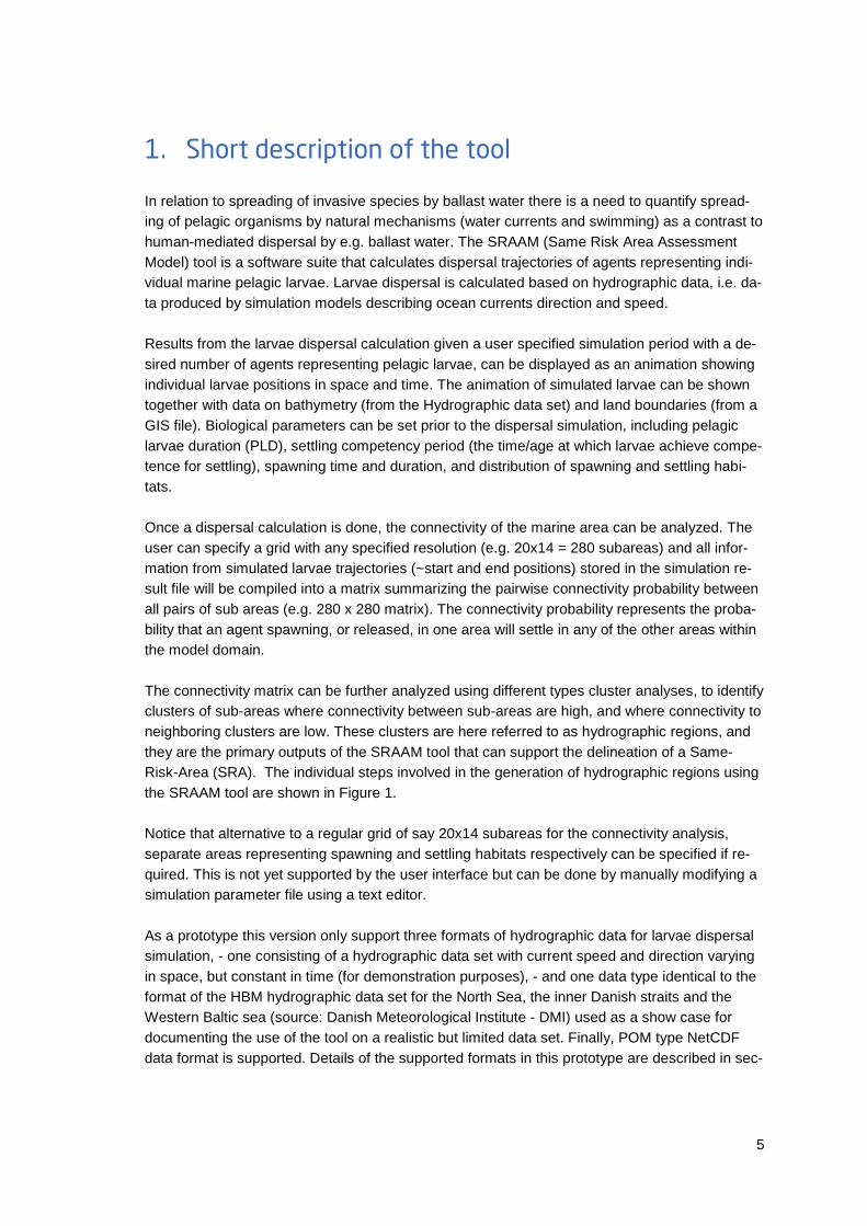
1. Short description of the tool In relation to spreading of invasive species by ballast water there is a need to quantify spread-ing of pelagic organisms by natural mechanisms (water currents and swimming) as a contrast to human-mediated dispersal by e.g. ballast water. The SRAAM (Same Risk Area Assessment Model) tool is a software suite that calculates dispersal trajectories of agents representing indi-vidual marine pelagic larvae. Larvae dispersal is calculated based on hydrographic data, i.e. da-ta produced by simulation models describing ocean currents direction and speed. Results from the larvae dispersal calculation given a user specified simulation period with a de-sired number of agents representing pelagic larvae, can be displayed as an animation showing individual larvae positions in space and time. The animation of simulated larvae can be shown together with data on bathymetry (from the Hydrographic data set) and land boundaries (from a GIS file). Biological parameters can be set prior to the dispersal simulation, including pelagic larvae duration (PLD), settling competency period (the time/age at which larvae achieve compe-tence for settling), spawning time and duration, and distribution of spawning and settling habi-tats. Once a dispersal calculation is done, the connectivity of the marine area can be analyzed. The user can specify a grid with any specified resolution (e.g. 20x14 = 280 subareas) and all infor-mation from simulated larvae trajectories (~start and end positions) stored in the simulation re-sult file will be compiled into a matrix summarizing the pairwise connectivity probability between all pairs of sub areas (e.g. 280 x 280 matrix). The connectivity probability represents the proba-bility that an agent spawning, or released, in one area will settle in any of the other areas within the model domain. The connectivity matrix can be further analyzed using different types cluster analyses, to identify clusters of sub-areas where connectivity between sub-areas are high, and where connectivity to neighboring clusters are low. These clusters are here referred to as hydrographic regions, and they are the primary outputs of the SRAAM tool that can support the delineation of a Same-Risk-Area (SRA). The individual steps involved in the generation of hydrographic regions using the SRAAM tool are shown in Figure 1. Notice that alternative to a regular grid of say 20x14 subareas for the connectivity analysis, separate areas representing spawning and settling habitats respectively can be specified if re-quired. This is not yet supported by the user interface but can be done by manually modifying a simulation parameter file using a text editor. As a prototype this version only support three formats of hydrographic data for larvae dispersal simulation, - one consisting of a hydrographic data set with current speed and direction varying in space, but constant in time (for demonstration purposes), - and one data type identical to the format of the HBM hydrographic data set for the North Sea, the inner Danish straits and the Western Baltic sea (source: Danish Meteorological Institute - DMI) used as a show case for documenting the use of the tool on a realistic but limited data set. Finally, POM type NetCDF data format is supported. Details of the supported formats in this prototype are described in sec-

6

tion “Hydrographic data”. Support for additional hydrographic formats may be implemented on demand.

Figure 1. Individual steps supported by the SRAAM tool: 1. Larvae dispersal simulation based on existing hy-

drographic data. 2. Area subdivision, - dividing the model domain into a regular grid or dividing the area into 2 irregular grids, 1 representing spawning habitats, and 1 representing settling habitats. 3. Generation of a con-

nectivity probability matrix. 4. Cluster analysis for dividing the model domain into hydrographic regions repre-

senting region of high connectivity within each region, and low connectivity between regions.

The animation of simulated larvae trajectories is mostly an option available for visualizing the dispersal patterns and drivers in the system analyzed, and should only be done using simulation results for relatively limited number of agents , e.g. ~ 100 - 1000 agents for 1 year simulation, due to pc-processing time and optimal visualization.

The SRAAM tool utilizes a combination of 3 freeware/open source programs:

- Netlogo – which is one of the most popular software programs for Agent-Based / Indi-vidual-based Modeling (Wilensky, U. 1999). NetLogo is used as GUI for setting up/analyzing simulations

- R – which is a popular software package for statistical and mathematical data analyses and processing (R Core Team 2013). R provides statistical cluster analyses of the con-nectivity matrix.

- IBMlib – This is a modelling system (~model library) specifically developed for linking agent-based simulations to simulated 3D hydrodynamic data (Christensen 2008, Chris-tensen et al. in review). It is used as calculation engine for agent-based simulations.

7

2. User interface

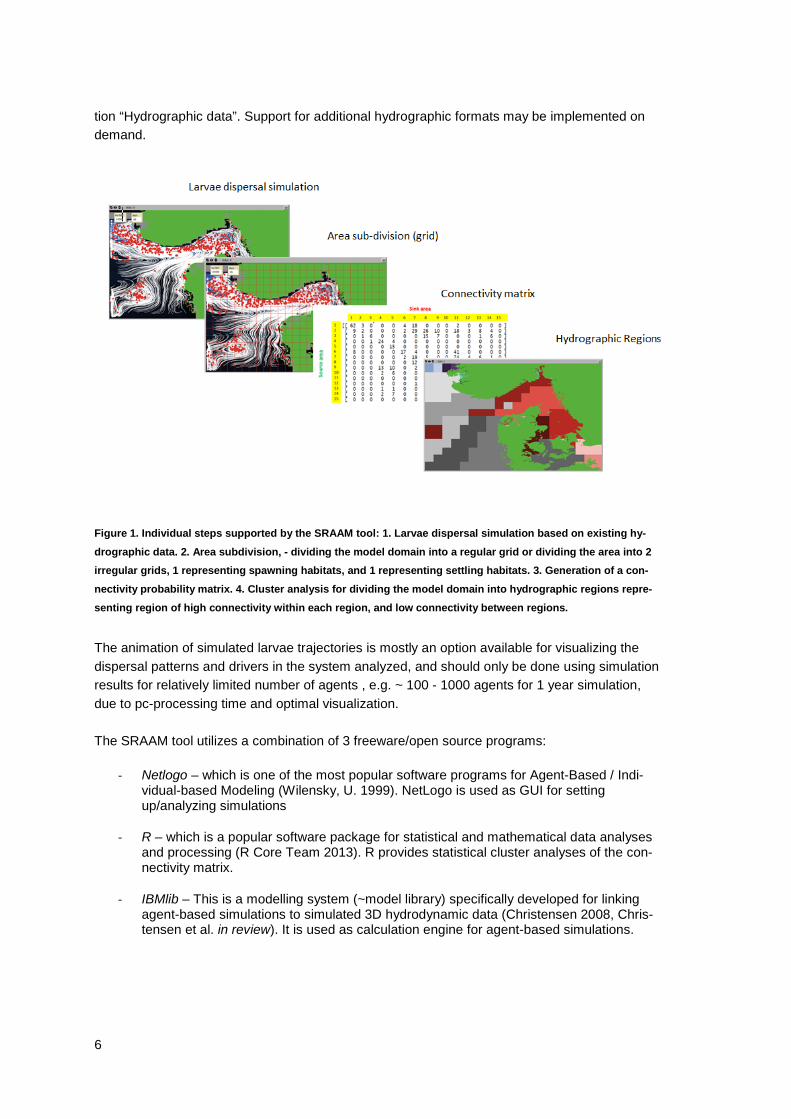
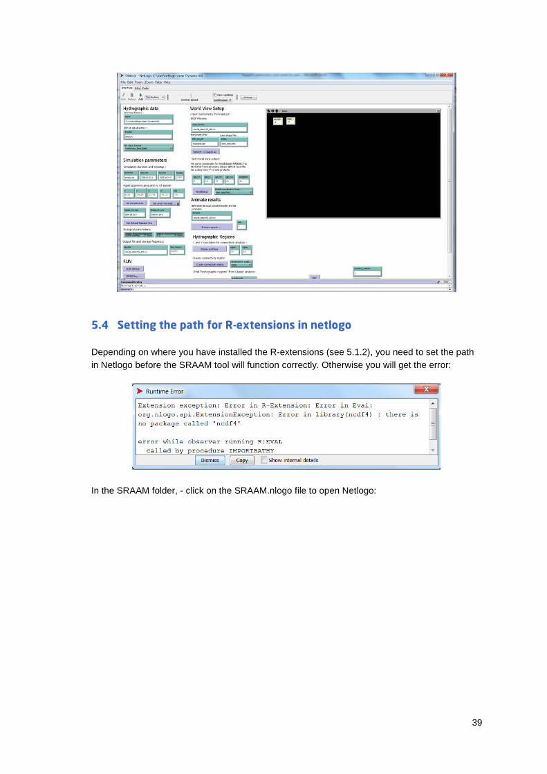
2.1 User interface overview The user interface for this SRAAM tool prototype is generated in Netlogo 5.3.1 using standard Netlogo interface components. All user inputs and displays are compiled within one single win-dow. No attempts have been done to hide un-necessary menus and graphical user interfaces, which may not be relevant for the use of the SRAAM tool. To get acquainted with the standard Netlogo user interface, please refer to the Netlogo Dictionary: file:///C:/Program%20Files/NetLogo%205.3.1/app/docs/index2.html.

Figure 2. The SRAAM tool Graphical User-Interface showing the Netlogo “interface” tab where all user inputs and result presentations are given/shown. Here the interface is divided into 4 main sections: 1. User input for

larvae dispersal calculation. 2. User input for result analysis, presentation and delineation of hydrographic re-

gions. 3 . World View – for displaying bathymetry data, land areas , larvae dispersal animations and hydro-graphic regions delineation.

In short, - apart from the upper standard program menu including “File” , “Edit” etc. the main program window include 3 tabs, - “Interface” , “info” and “code”. The former (figure 2) is the in-

8

terface from where all SRAAM tool operations are done. The latter is where all code is written associated with buttons, sliders, data-input boxes etc. The user inteface developed for the SRAAM tool including larvae dispersal simulations and delineation of hydrographic regions can be divided into three main sections (figure 2):

1. User inputs for larvae dispersal calculation2. User inputs for result presentation and delineation of hydrographic regions3. World View – for displaying bathymetry data, land areas, larvae dispersal animation and

hydrographic region delineation.

In addition to these tool specific sections, - the lower part of the progam window consist of the Netlogo “control center”. Here progress and information during SRAAM tool execusions are shown. Also if some error may occurs.

2.2 User input for larvae dispersal calculation The user input for larvae dispersal calculation are further divided into 3 sub-sections:

- Hydrographic data – where working directories are set and where the hydrographic data format is chosen.

- Simulation parameters – where all paramters and setting for the larvae dispersal simulation are specified

- RUN – where the larvae dispersal simulation is executed.

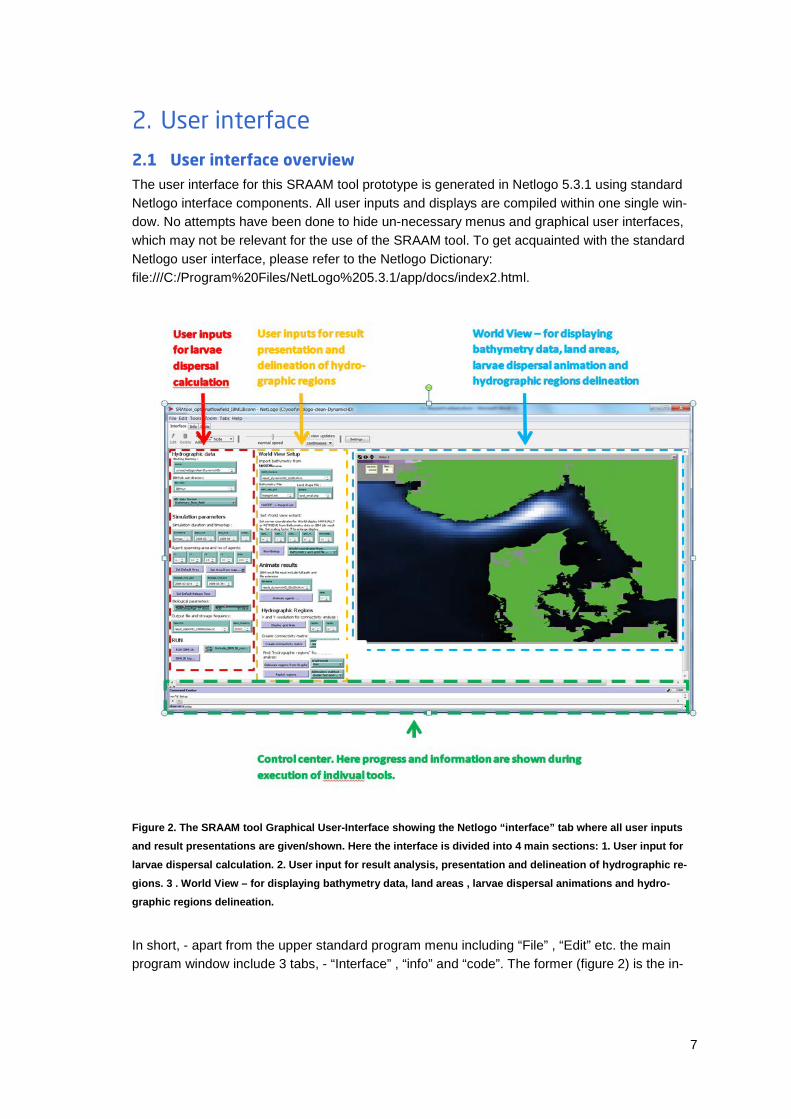
2.2.1 Hydrographic data

The “hydrographic data” section requires 3 user inputs:

1. Working directory2. IBMLib Sub-directory3. HD data Format

9

Working directory A full path of the working directory must be specified. The working directory refers to the folder where all files generated by the SRAAM tool will be located, such as the Netlogo project file (*.nlogo) and R-script files (*.r). Any GIS polygon files representing land areas (*.shp) or grid bathymetry files (*.asc) must be placed here.

IBMLib sub-directory In addition to the working directory a sub-directory name must be specified, i.e. a sub-folder where all files related to the IBMLib will be stored including sub-folders for each set of hydro-graphic data. Format of the hydrographic data sets, please see chapter 2.4. In this folder the IMBrun_connect_xxx.exe file must be located. This is the file that the SRAAM tool calls when larvae dispersal calculations are executed. Notice that there will be an IMBrun_connect_xxx.exe file for each hydrographic data format supported (e.g. IBMrun_connect_HBM.exe, IBMrun_connect_bootHD.exe, IBMrun_connect_POMtype.exe). The IBMrun_connect_xxx.exe file require an input parameter file (e.g. simpar.txt) which will be automatically generated from the user input in the “simulation parameters” section (see later) once you press the “RUN” but-ton for execution of the larvae dispersal simulation.

Hydrographic data format In the current prototype, only 2 types of hydrographic data are supported:

1. Static flow field2. Dynamic flow field (HBM)3. POM type flow fields

Static flow field: This data consists of a hydrographic data set with current speed and direction varying in space, but constant in time. This data is included for demonstration purposes. Since data do not vary in time, the larvae dispersal calculation execution is fast. It must be empha-sized that a static flow field is not a realistic data set and should be regarded as a data set pri-marily for demonstrating the capability of the SRAAM tool or quick test runs of a given setup.

Dynamic flow field (HBM): This data format is identical to the format of the HBM hydrographic data set for the North Sea, the inner Danish straits and the Western Baltic sea (source: DMI1) used as a show case for documenting the use of the SRAAM tool on a realistic but limited data set. Details of this supported format in this prototype are described in section 2.4. Time varying 3D hydrodynamic data files for larger areas and for realistic periods are large (>> 1 GB) and thus only a few days of this data source has been included in this SRAAM tool prototype for download.

POM type flow field): This data format is derived from a POM type setup and is described later in section 3.2. The format is rather simple and can potentially be used as target format to recast another type dynamic flow field.

1 http://ocean.dmi.dk/models/hbm.uk.php

10

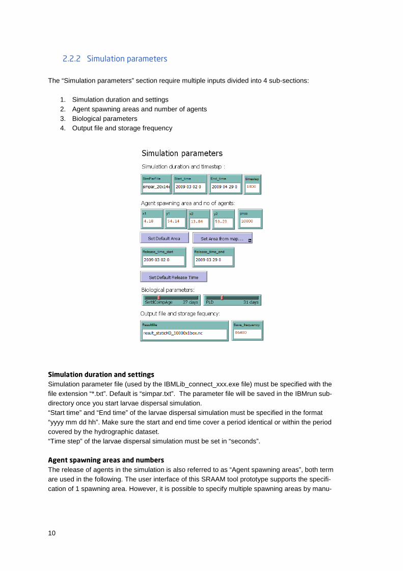
2.2.2 Simulation parameters

The “Simulation parameters” section require multiple inputs divided into 4 sub-sections:

1. Simulation duration and settings2. Agent spawning areas and number of agents3. Biological parameters4. Output file and storage frequency

Simulation duration and settings Simulation parameter file (used by the IBMLib_connect_xxx.exe file) must be specified with the file extension “*.txt”. Default is “simpar.txt”. The parameter file will be saved in the IBMrun sub-directory once you start larvae dispersal simulation. “Start time” and “End time” of the larvae dispersal simulation must be specified in the format “yyyy mm dd hh”. Make sure the start and end time cover a period identical or within the period covered by the hydrographic dataset. “Time step” of the larvae dispersal simulation must be set in “seconds”.

Agent spawning areas and numbers The release of agents in the simulation is also referred to as “Agent spawning areas”, both term are used in the following. The user interface of this SRAAM tool prototype supports the specifi-cation of 1 spawning area. However, it is possible to specify multiple spawning areas by manu-

11

ally updating the simulation parameter file, see later. There are 3 ways to set the spawning ar-ea using the user interface:

1. Manually type in the geographical coordinates of the lower left (x1, y1) and upper right(x2, y2) corners of a rectangle representing the release area. Make sure the coordi-nates lye within the model domain.

2. Use the “Set Default Area” which will set the lower left and upper right corner coordi-nates to the corner coordinates of the model domain.

3. Use the “Set Area from map…” which enables the user to interactively click on the“World View” to retrieve first the lower left and secondly upper right corner coordinates.This requires that the World View has been setup (see section 2.3.1). The first click hasto be the coordinate of the lower left corner!

Using the latter 2 options, the corner coordinates will be updated in the input boxes, i.e. x1, y1, x2 and y2.

The total number (integer) of agents released within the area covered by the specified rectangle must be specified in the “pnos” input box.

The time period for agent release has to be set by specifying a “Release time start” and a “Re-lease time end”. The time format is “yyyy mm dd h”.

Agents will be randomly distributed in space and time: i.e. within the specified spawning area (= rectangle) and within the specified release period.

When using the SRAAM tool GUI as described here, all agents are assumed to be able to settle in the area identical to the specified spawning/release area.

Option for Multiple spawning areas

An option for multiple spawning areas is possible but not supported by the user interface of this prototype. Multiple spawning areas is a relevant option if you want to distribute agents irregular-ly in the model domain, for instance limited to specific spawning areas and/or with varying den-sities.

Multiple spawning areas can be included by manually adding a list of corner coordinates in the “simpar.txt” file by opening the file using a text editor.

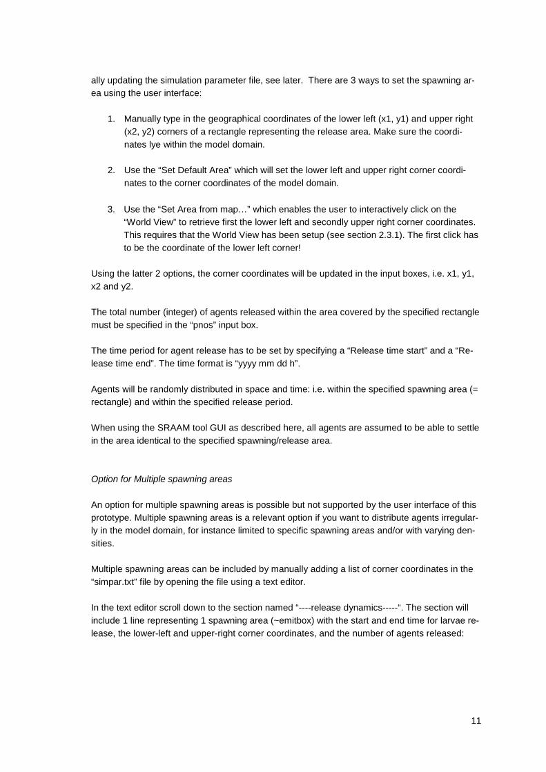
In the text editor scroll down to the section named “----release dynamics-----“. The section will include 1 line representing 1 spawning area (~emitbox) with the start and end time for larvae re-lease, the lower-left and upper-right corner coordinates, and the number of agents released:

12

When applying multiple release areas, simply copy and paste the line and modify the release time, release corner coordinates and the number of agents to be released:

Option for including settling areas

In the simulation parameter file (simpar.txt) below the section “release dynamics”, a section is available for “settlement dynamics”. In this section, areas representing larvae settlement habi-tats can be specified. This option is relevant if you want to simulate a scenario where larvae are released from one type of habitats (or specific ballast water release locations) and where the larvae will only be able to settle successfully in a specific and different habitat. In such a scenar-io you will need to manually specify a set of spawning areas (see above), and a set of settle-ment areas. IBMlib will then calculate a connectivity matrix describing the connectivity probabil-ity between each spawning area and each settlement area.

Settlement areas are specified similar to spawning areas described above including information on lower-left and upper-right corner coordinates of each settlement area:

To include the connectivity matrix calculated by IBMLib at the end of each simulation, in the simulation result file (*.nc) the section below needs to be present in the simpar.txt file:

13

At this stage of the SRAAM tool development there is no further cluster or network analysis im-plemented to evaluate these results linking spawning/release areas to settlement areas. How-ever, the IBMlib generated connectivity matrix can be imported into R using the R extension NCDF4 and subsequently analysed manually in R or some other system.

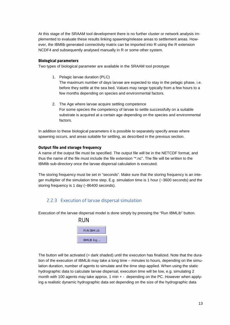
Biological parameters Two types of biological parameter are available in the SRAAM tool prototype:

1. Pelagic larvae duration (PLC)The maximum number of days larvae are expected to stay in the pelagic phase, i.e.before they settle at the sea bed. Values may range typically from a few hours to afew months depending on species and environmental factors.

2. The Age where larvae acquire settling competenceFor some species the competency of larvae to settle successfully on a suitablesubstrate is acquired at a certain age depending on the species and environmentalfactors.

In addition to these biological parameters it is possible to separately specify areas where spawning occurs, and areas suitable for settling, as described in the previous section.

Output file and storage frequency A name of the output file must be specified. The output file will be in the NETCDF format, and thus the name of the file must include the file extension “*.nc”. The file will be written to the IBMlib sub-directory once the larvae dispersal calculation is executed.

The storing frequency must be set in “seconds”. Make sure that the storing frequency is an inte-ger multiplier of the simulation time step. E.g. simulation time is 1 hour (~3600 seconds) and the storing frequency is 1 day (~86400 seconds).

2.2.3 Execution of larvae dispersal simulation

Execution of the larvae dispersal model is done simply by pressing the “Run IBMLib” button.

The button will be activated (= dark shaded) until the execution has finalized. Note that the dura-tion of the execution of IBMLib may take a long time – minutes to hours, depending on the simu-lation duration, number of agents to simulate and the time step applied. When using the static hydrographic data to calculate larvae dispersal, execution time will be low, e.g. simulating 2 month with 100 agents may take approx. 1 min + - depending on the PC. However when apply-ing a realistic dynamic hydrographic data set depending on the size of the hydrographic data

14

files, execution time may be significantly longer, - minutes to hours. This prototype does not in-clude any information on the progress of the IBMLib calculation. However, it is possible to open a simulation log file, and scroll to the end of the file and notice the latest time step. This file is continuously updated and thus can provide an approximate info on execution progress. The log file “stdout.txt” is located in the IBMrun-subdirectory.

Figure 3. The time step progress of the IBMLib execution written to the IBMLib simulation log file “sdout.txt”.

Once the IBMLib execution has finished, the Run IBMlib button will change to “unshaded” and to inspect the IBMlib log, click the “IBMLib log …” and the last 20 lines in the IBMlib log file will be displayed in the Netlogo command center. This option is usefull if the IBMlib simulation ter-minates before starting, - and may provide some information on the reason for IBMlib being un-able to start. If the log is empty the run was not initiated properly. To view the entire log e.g. of successful simulation or a simulation where an error occurs after simulation has been initiated but fails to end successfully, open the log file “stdout.txt” in a text editor, e.g. Notepad++.

2.3 User input for result presentation and analysis

2.3.1 World View Setup Before any visualization of larvae dispersal trajectories or delineation of hydrographic regions can be done, the World View needs to be setup to cover the model domain, or part of the model domain. Notice that coordinates are assumed to be in geographical coordinates.

This section includes two subsections:

1. Import Bathymtry data from NetCDF result file2. Setting world extend

15

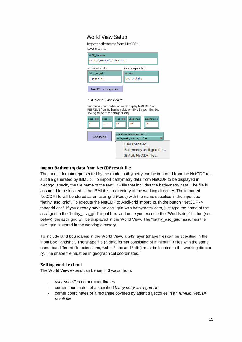
Import Bathymtry data from NetCDF result file The model domain represented by the model bathymetry can be imported from the NetCDF re-sult file generated by IBMLib. To import bathymetry data from NetCDF to be displayed in Netlogo, specify the file name of the NetCDF file that includes the bathymetry data. The file is assumed to be located in the IBMLib sub-directory of the working directory. The imported NetCDF file will be stored as an ascii-grid (*.asc) with the name specified in the input box “bathy_asc_grid”. To execute the NetCDF to Ascii-grid import, push the button “NetCDF -> topogrid.asc”. If you already have an ascii grid with bathymetry data, just type the name of the ascii-grid in the “bathy_asc_grid” input box, and once you execute the “Worldsetup” button (see below), the ascii grid will be displayed in the World View. The “bathy_asc_grid” assumes the ascii grid is stored in the working directory.

To include land boundaries in the World View, a GIS layer (shape file) can be specified in the input box “landshp”. The shape file (a data format consisting of minimum 3 files with the same name but different file extensions, *.shp, *.shx and *.dbf) must be located in the working directo-ry. The shape file must be in geographical coordinates.

Setting world extend The World View extend can be set in 3 ways, from:

- user specified corner coordinates - corner coordinates of a specified bathymetry ascii grid file - corner coordinates of a rectangle covered by agent trajectories in an IBMLib NetCDF

result file

16

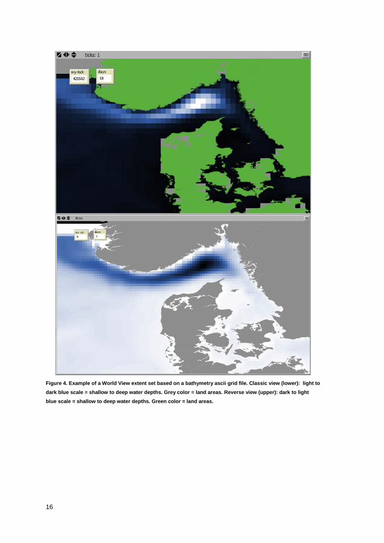
Figure 4. Example of a World View extent set based on a bathymetry ascii grid file. Classic view (lower): light to

dark blue scale = shallow to deep water depths. Grey color = land areas. Reverse view (upper): dark to light

blue scale = shallow to deep water depths. Green color = land areas.

17

First select which of the 3 methods to use, - select from the pull down menu “World-coordinates-from…”.

To set the World View extent manually, select “User specified…”, and simply type in the geographical coordinates of the lower left (xgeo_min, ygeo_min) and upper right (xgeo_max, ygeo_max) corners of the world view extent.

To set the World View from a specified bathymetry file, select “Bathymetry ascii grid file…”. This option will use the corner coordinates of the bathymetry ascii grid file specified in the “bathy_asc_grid” input box, as described above.

To set the World View from an “IBMLib NetCDF result file, select “IBMLib NetCDF file…”. This option will use the corner coordinates of the IBMLib result file specified in the “Animate Results” section, see section 2.3.2 below.

To setup the World View from the World View extent method selected above, click the button “Worldsetup” and the World View will be updated (see figure 4).

A scaling factor can be applied to increase or decrease the world view extent to fit the pc screen as required. Setting the “Scaling factor” to any integer will multiply the World View extent in the x and y dimenstion respectively. As a start set the factor to 1, then gradually increase the factor to increase the visual extent. A too large value may stall Netlogo and you will need to restart.

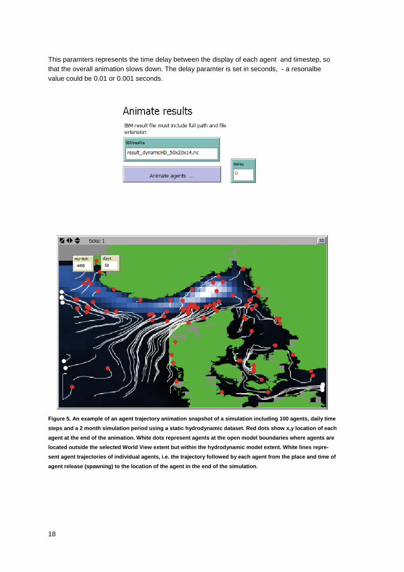
2.3.2 Animation of larvae dispersal To animate simulated agent trajectories in the World View, simply spedify the IBMLib NetCDF file (*.nc) to be animated in the “IBMresfile” input box in the “Animate results” section, and click the button “Animate agents … “. The World View will be updated and agent trajectories displayed (e.g. figure 5). For large data files with large numbers of agents (e.g. >= 1000 agents) this may take a considerable time. Thus, it is recommended for animation purposes to only include a limited number of agents in the simulation (e.g. <= 1000 agents). To reduce the time for reading the IBMLib result files, the “storing frequency” in the “Simulation parameters” section, can be set to 1 day (= 86400 seconds) instead of e.g. hours or minutes. For small result files (e.g. < 100 agents) and with a storing frequency of e.g. daily timesteps the animation may be displayed too fast for a meaningfull visual inspection. In this case a “delay” paramter can be set.

18

This paramters represents the time delay between the display of each agent and timestep, so that the overall animation slows down. The delay paramter is set in seconds, - a resonalbe value could be 0.01 or 0.001 seconds.

Figure 5. An example of an agent trajectory animation snapshot of a simulation including 100 agents, daily time

steps and a 2 month simulation period using a static hydrodynamic dataset. Red dots show x,y location of each

agent at the end of the animation. White dots represent agents at the open model boundaries where agents are located outside the selected World View extent but within the hydrodynamic model extent. White lines repre-

sent agent trajectories of individual agents, i.e. the trajectory followed by each agent from the place and time of

agent release (spawning) to the location of the agent in the end of the simulation.

19

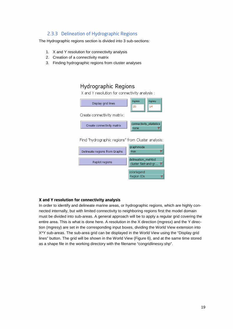
2.3.3 Delineation of Hydrographic Regions The Hydrographic regions section is divided into 3 sub-sections:

1. X and Y resolution for connectivity analysis2. Creation of a connectivity matrix3. Finding hydrographic regions from cluster analyses

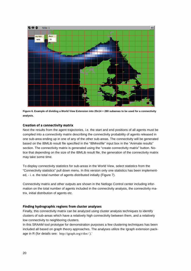
X and Y resolution for connectivity analysis In order to identify and delineate marine areas, or hydrographic regions, which are highly con-nected internally, but with limited connectivity to neighboring regions first the model domain must be divided into sub-areas. A general approach will be to apply a regular grid covering the entire area. This is what is done here. A resolution in the X direction (mgresx) and the Y direc-tion (mgresy) are set in the corresponding input boxes, dividing the World View extension into X*Y sub-areas. The sub-area grid can be displayed in the World View using the “Display grid lines” button. The grid will be shown in the World View (Figure 6), and at the same time stored as a shape file in the working directory with the filename “congridlinesxy.shp”.

20

Figure 6. Example of dividing a World View Extension into 20x14 = 280 subareas to be used for a connectivity analysis.

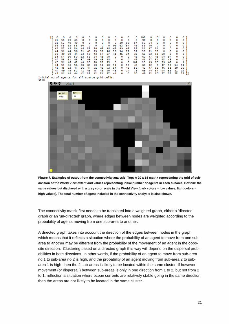
Creation of a connectivity matrix Next the results from the agent trajectories, i.e. the start and end positions of all agents must be compiled into a connectivity matrix describing the connectivity probability of agents released in one sub-area ending up in one of any of the other sub-areas. The connectivity will be generated based on the IBMLib result file specified in the “IBMresfile” input box in the “Animate results” section. The connectivity matrix is generated using the “create connectivity matrix” button. No-tice that depending on the size of the IBMLib result file, the generation of the connectivity matrix may take some time. To display connectivity statistics for sub-areas in the World View, select statistics from the “Connectivity statistics” pull down menu. In this version only one statistics has been implement-ed, - i. e. the total number of agents distributed initially (Figure 7). Connectivity matrix and other outputs are shown in the Netlogo Control center including infor-mation on the total number of agents included in the connectivity analysis, the connectivity ma-trix, initial distribution of agents etc. Finding hydrographic regions from cluster analyses Finally, this connectivity matrix can be analyzed using cluster analysis techniques to identify clusters of sub-areas which have a relatively high connectivity between them, and a relatively low connectivity to neighboring clusters. In this SRAAM tool prototype for demonstration purposes a few clustering techniques has been included all based on graph theory approaches. The analyses utilize the Igraph extension pack-age in R (for details see: http://igraph.org/r/doc/ ).’

21

Figure 7. Examples of output from the connectivity analysis. Top: A 20 x 14 matrix representing the grid of sub-

division of the World View extent and values representing initial number of agents in each subarea. Bottom: the same values but displayed with a grey color scale in the World View (dark colors = low values, light colors =

high values). The total number of agent included in the connectivity analysis is also shown.

The connectivity matrix first needs to be translated into a weighted graph, either a ‘directed’ graph or an ‘un-directed’ graph, where edges between nodes are weighted according to the probability of agents moving from one sub-area to another. A directed graph takes into account the direction of the edges between nodes in the graph, which means that it reflects a situation where the probability of an agent to move from one sub-area to another may be different from the probability of the movement of an agent in the oppo-site direction. Clustering based on a directed graph this way will depend on the dispersal prob-abilities in both directions. In other words, if the probability of an agent to move from sub-area no.1 to sub-area no.2 is high, and the probability of an agent moving from sub-area 2 to sub-area 1 is high, then the 2 sub-areas is likely to be located within the same cluster. If however movement (or dispersal ) between sub-areas is only in one direction from 1 to 2, but not from 2 to 1, reflection a situation where ocean currents are relatively stable going in the same direction, then the areas are not likely to be located in the same cluster.

22

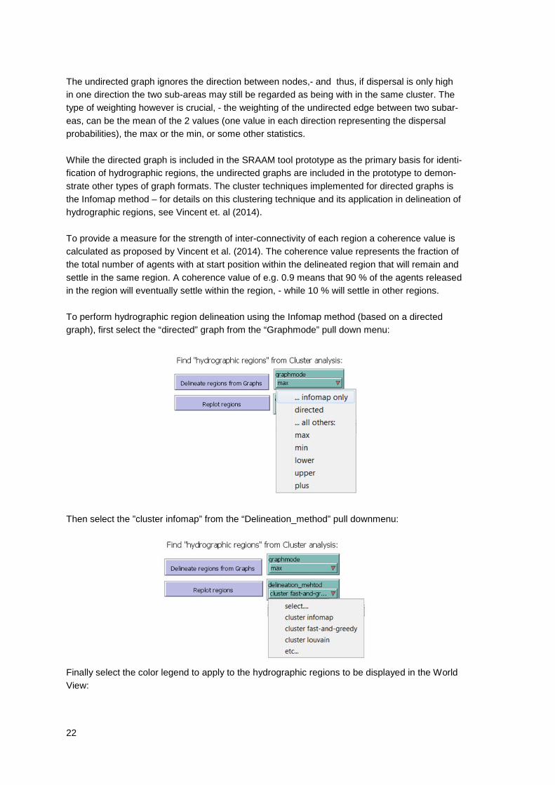
The undirected graph ignores the direction between nodes,- and thus, if dispersal is only high in one direction the two sub-areas may still be regarded as being with in the same cluster. The type of weighting however is crucial, - the weighting of the undirected edge between two subar-eas, can be the mean of the 2 values (one value in each direction representing the dispersal probabilities), the max or the min, or some other statistics. While the directed graph is included in the SRAAM tool prototype as the primary basis for identi-fication of hydrographic regions, the undirected graphs are included in the prototype to demon-strate other types of graph formats. The cluster techniques implemented for directed graphs is the Infomap method – for details on this clustering technique and its application in delineation of hydrographic regions, see Vincent et. al (2014). To provide a measure for the strength of inter-connectivity of each region a coherence value is calculated as proposed by Vincent et al. (2014). The coherence value represents the fraction of the total number of agents with at start position within the delineated region that will remain and settle in the same region. A coherence value of e.g. 0.9 means that 90 % of the agents released in the region will eventually settle within the region, - while 10 % will settle in other regions. To perform hydrographic region delineation using the Infomap method (based on a directed graph), first select the “directed” graph from the “Graphmode” pull down menu:

Then select the ”cluster infomap” from the “Delineation_method” pull downmenu:

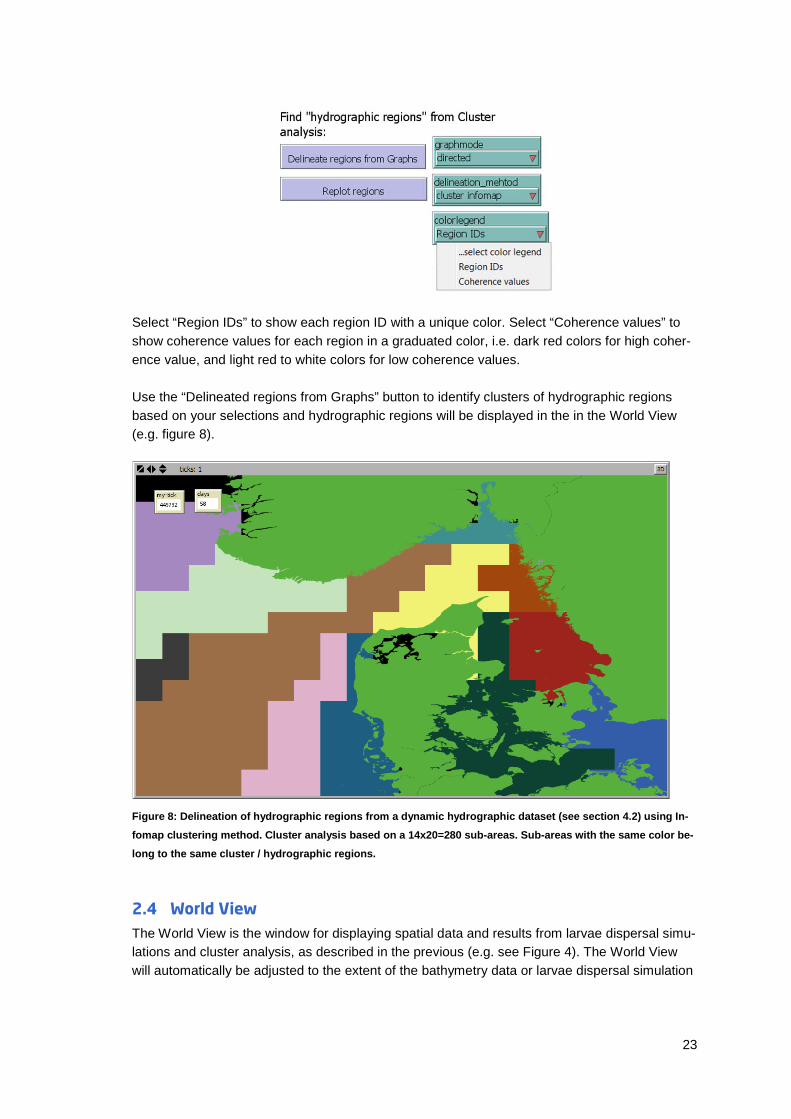
Finally select the color legend to apply to the hydrographic regions to be displayed in the World View:

23

Select “Region IDs” to show each region ID with a unique color. Select “Coherence values” to show coherence values for each region in a graduated color, i.e. dark red colors for high coher-ence value, and light red to white colors for low coherence values. Use the “Delineated regions from Graphs” button to identify clusters of hydrographic regions based on your selections and hydrographic regions will be displayed in the in the World View (e.g. figure 8).

Figure 8: Delineation of hydrographic regions from a dynamic hydrographic dataset (see section 4.2) using In-

fomap clustering method. Cluster analysis based on a 14x20=280 sub-areas. Sub-areas with the same color be-

long to the same cluster / hydrographic regions.

2.4 World View The World View is the window for displaying spatial data and results from larvae dispersal simu-lations and cluster analysis, as described in the previous (e.g. see Figure 4). The World View will automatically be adjusted to the extent of the bathymetry data or larvae dispersal simulation

24

result files, i.e the extent covered by the geographical datasets. Bathymetry data is here shown in a blue-white color scale with increasing depth with increasing darkness (classic view) or the reverse (reverse view). Land areas are shown in grey (classic view) or green (reverse view). In the upper left corner a “tick” counter and a “days” counter is placed. These are only relevant for animation of larvae dispersal sTicks counts each combination of agents and timestep, while days counts each day in the simulation results.

25

3. Hydrographic data formats The normal way to interface IBMlib with a new hydrographic format is to add a new physical interface layer that couples the data set to IBMlib. This procedure does not require reformatting of the hydrographic data set, but IBMlib can then read data as-provided. Alternatively, one can recast a new hydrographic data set into a format corresponding to an already implemented interface; this alternative should be pursued with caution, because (i) recasting may involve numerical truncation and thus accuracy loss and (ii) recasting may be faulty because the translator either have misunderstood the native hydrographic format or the format specification and (iii) some special features of the hydrographic data set may be lost because it can not be represented by the target format. Extensive testing is therefore recommended before actual result generating runs are performed. The suggested target format for recasting is based on the POM output layout (Princeton Ocena Model, see http://www.ccpo.odu.edu/POMWEB/), which is relatively simple and transparent; the abundance of regional POM setups also gives a chance that very little data transformation actually has to be done, if you are lucky. The format will support many typical usages of IBMlib. The target grid is regular longitude-latitude (with arbitrary user provided longitude-latitude spacing), vertically sigma-type (with number of layers specified by user), dynamic sea-level elevation and arbitrary topography. Data is stored as daily averaged hydrography frames with a filename corresponding to the date. The format is stored in netCDF (see http://www.unidata.ucar.edu/software/netcdf/) and consists of (1) A grid desciptor file "grid.nc" (2) A sequence of daily hydrography frames with filename "hydrography_YYYY_MM_DD.nc"

where (YYYY, MM, DD) is year, month and day-in-month number, respectively, with prepended zeroes as necessary, i.e. hydrography for February 15 2016 should be stored in file "hydrography_2016_02_15.nc". For convenience, the grid desciptor file may be merged with each hydrography file, but this requires a little extra storage, because the grid desciptor is duplicated many times. The templates for grid desciptor and hydrography frames are provided "grid.CDL" and "hydrography_YYYY_MM_DD.CDL". CDL is the text translation of netCDF, so these files show exactly what IBMlib expects - just show the CDL file to your hydrography data pusher. The period where you can conduct simulations correspond to the period covered by files hydrography_YYYY_MM_DD.nc. At runtime IBMlib tries to read the needed files hydrography_YYYY_MM_DD.nc and stops, if the file is not found (with the expected filename in the expected folder). You don't have to structure or declare the hydrographic database further, just place expected files in the path announced in the simulation input file with the proper names hydrography_YYYY_MM_DD.nc. If the format for one reason or another does not support your specific needs, it is recommended that you follow instructions within IBMlib for creating a specific physical interface for the data set and recompile IBMlib for your setup. IBMlib is free and open source, but if fortran programming and code compilation is a dangerous animal to you, you may contact the IBMlib developers to explore possibilities and conditions for a collaboration. Below you will find the content of "grid.CDL" and "hydrography_YYYY_MM_DD.CDL" that can be copied and pasted into a plain text file, if needed.

26

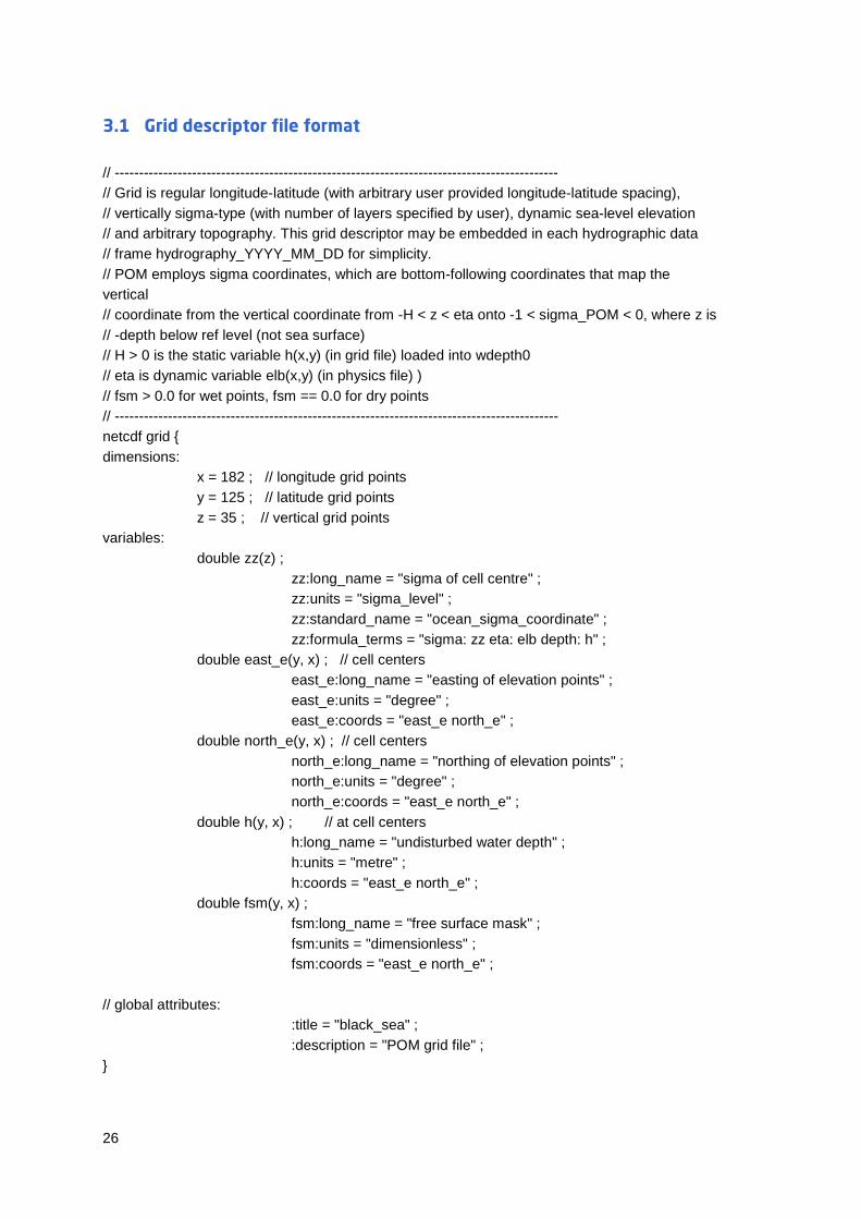
3.1 Grid descriptor file format // -------------------------------------------------------------------------------------------- // Grid is regular longitude-latitude (with arbitrary user provided longitude-latitude spacing), // vertically sigma-type (with number of layers specified by user), dynamic sea-level elevation // and arbitrary topography. This grid descriptor may be embedded in each hydrographic data // frame hydrography_YYYY_MM_DD for simplicity. // POM employs sigma coordinates, which are bottom-following coordinates that map the vertical // coordinate from the vertical coordinate from -H < z < eta onto -1 < sigma_POM < 0, where z is // -depth below ref level (not sea surface) // H > 0 is the static variable h(x,y) (in grid file) loaded into wdepth0 // eta is dynamic variable elb(x,y) (in physics file) ) // fsm > 0.0 for wet points, fsm == 0.0 for dry points // -------------------------------------------------------------------------------------------- netcdf grid { dimensions: x = 182 ; // longitude grid points y = 125 ; // latitude grid points z = 35 ; // vertical grid points variables: double zz(z) ; zz:long_name = "sigma of cell centre" ; zz:units = "sigma_level" ; zz:standard_name = "ocean_sigma_coordinate" ; zz:formula_terms = "sigma: zz eta: elb depth: h" ; double east_e(y, x) ; // cell centers east_e:long_name = "easting of elevation points" ; east_e:units = "degree" ; east_e:coords = "east_e north_e" ; double north_e(y, x) ; // cell centers north_e:long_name = "northing of elevation points" ; north_e:units = "degree" ; north_e:coords = "east_e north_e" ; double h(y, x) ; // at cell centers h:long_name = "undisturbed water depth" ; h:units = "metre" ; h:coords = "east_e north_e" ; double fsm(y, x) ; fsm:long_name = "free surface mask" ; fsm:units = "dimensionless" ; fsm:coords = "east_e north_e" ; // global attributes: :title = "black_sea" ; :description = "POM grid file" ; }

27

3.2 Hydrographic data format // ------------------------------------------------------------------------------ // POM employs sigma coordinates, which are bottom-following coordinates that map the // vertical coordinate from the vertical coordinate from -H < z < eta onto -1 < sigma_POM < 0, / // where z is -depth below ref level (not sea surface) // H > 0 is the static variable h(x,y) (in grid file) loaded into wdepth0 eta is dynamic variable // elb(x,y) (in physics file) ) // nz is number of faces vertically so that the number of wet cells is nz-1 vertically. // Cell-centered arrays like t (temperature) are padded with an arbitrary value in last // element iz=35 (surface cell at iz=1) // netCDF variable w(x,y,z) refers to vertical faces (not cell centers), so w(x,y,1) ~ 0 // at sea surface and w(x,y,nz=35) = 0 at the sea bed. // Currently load these fields (in native units/conventions, c-declaration index order): // float elb(y, x) = "surface elevation in external mode at -dt" units = "metre" ; // staggering = (east_e, north_e) // float u(z, y, x) = "x-velocity" units = "metre/sec" ; // staggering = (east_u, north_u, zz) // float v(z, y, x) = "y-velocity" units = "metre/sec" ; // staggering = (east_v, north_v, zz) // float w(z, y, x) = "sigma-velocity" units = "metre/sec" ; // staggering = (east_e, north_e, z) // float t(z, y, x) = "potential temperature" ; units = "K" ; // staggering = (east_e, north_e, zz) // float s(z, y, x) = "salinity x rho / rhoref" ; units = "PSS" ; // staggering = (east_e, north_e, zz) // float rho(z, y, x) = "(density-1000)/rhoref" ; units = "dimless" // staggering = (east_e, north_e, zz) // float kh(z, y, x) = "vertical diffusivity" ; units = "m^2/sec"; // staggering = (east_e, north_e, zz) // float aam(z, y, x) = "horizontal kinematic viscosity" ; units = "metre^2/sec"; // staggering = (east_e, north_e, zz) // u(ix,iy,iz) in grid position (ix-0.5, iy , iz) (i.e. western cell face) // v(ix,iy,iz) in grid position (ix , iy-0.5, iz) (i.e. southern cell face) // w(ix,iy,iz) in grid position (ix , iy, iz-0.5) (i.e. upper cell face) // The boundary condition: w( ix, iy, nz+0.5 ) = 0 is implicit // ------------------------------------------------------------------------------ netcdf hydrography_YYYY_MM_DD { dimensions: z = 35 ; y = 125 ; x = 182 ; variables: float elb(y, x) ; elb:long_name = "surface elevation in external mode at -dt" ; elb:units = "metre" ; elb:coordinates = "east_e north_e" ;

28

float u(z, y, x) ; u:long_name = "x-velocity" ; u:units = "metre/sec" ; u:coordinates = "east_u north_u zz" ; float v(z, y, x) ; v:long_name = "y-velocity" ; v:units = "metre/sec" ; v:coordinates = "east_v north_v zz" ; float w(z, y, x) ; w:long_name = "sigma-velocity" ; w:units = "metre/sec" ; w:coordinates = "east_e north_e zz" ; float t(z, y, x) ; t:long_name = "potential temperature" ; t:units = "K" ; t:coordinates = "east_e north_e zz" ; float s(z, y, x) ; s:long_name = "salinity x rho / rhoref" ; s:units = "PSS" ; s:coordinates = "east_e north_e zz" ; float rho(z, y, x) ; rho:long_name = "(density-1000)/rhoref" ; rho:units = "dimensionless" ; rho:coordinates = "east_e north_e zz" ; float kh(z, y, x) ; kh:long_name = "vertical diffusivity" ; kh:units = "metre^2/sec" ; kh:coordinates = "east_e north_e zz" ; float aam(z, y, x) ; aam:long_name = "horizontal kinematic viscosity" ; aam:units = "metre^2/sec" ; aam:coordinates = "east_e north_e zz" ; // global attributes: :title = "black_sea" ; :description = "restart file" ; }

29

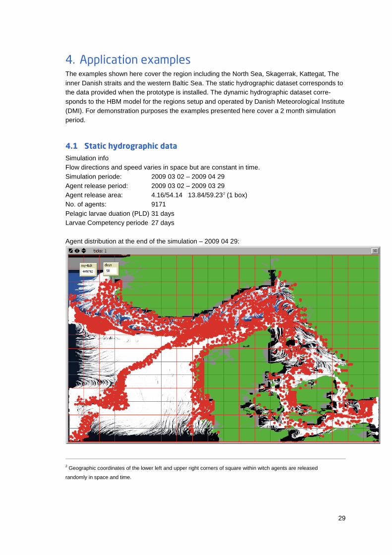
4. Application examples The examples shown here cover the region including the North Sea, Skagerrak, Kattegat, The inner Danish straits and the western Baltic Sea. The static hydrographic dataset corresponds to the data provided when the prototype is installed. The dynamic hydrographic dataset corre-sponds to the HBM model for the regions setup and operated by Danish Meteorological Institute (DMI). For demonstration purposes the examples presented here cover a 2 month simulation period.

4.1 Static hydrographic data Simulation info Flow directions and speed varies in space but are constant in time. Simulation periode: 2009 03 02 – 2009 04 29 Agent release period: 2009 03 02 – 2009 03 29 Agent release area: 4.16/54.14 13.84/59.232 (1 box) No. of agents: 9171 Pelagic larvae duation (PLD) 31 days Larvae Competency periode 27 days Agent distribution at the end of the simulation – 2009 04 29:

2 Geographic coordinates of the lower left and upper right corners of square within witch agents are released

randomly in space and time.

30

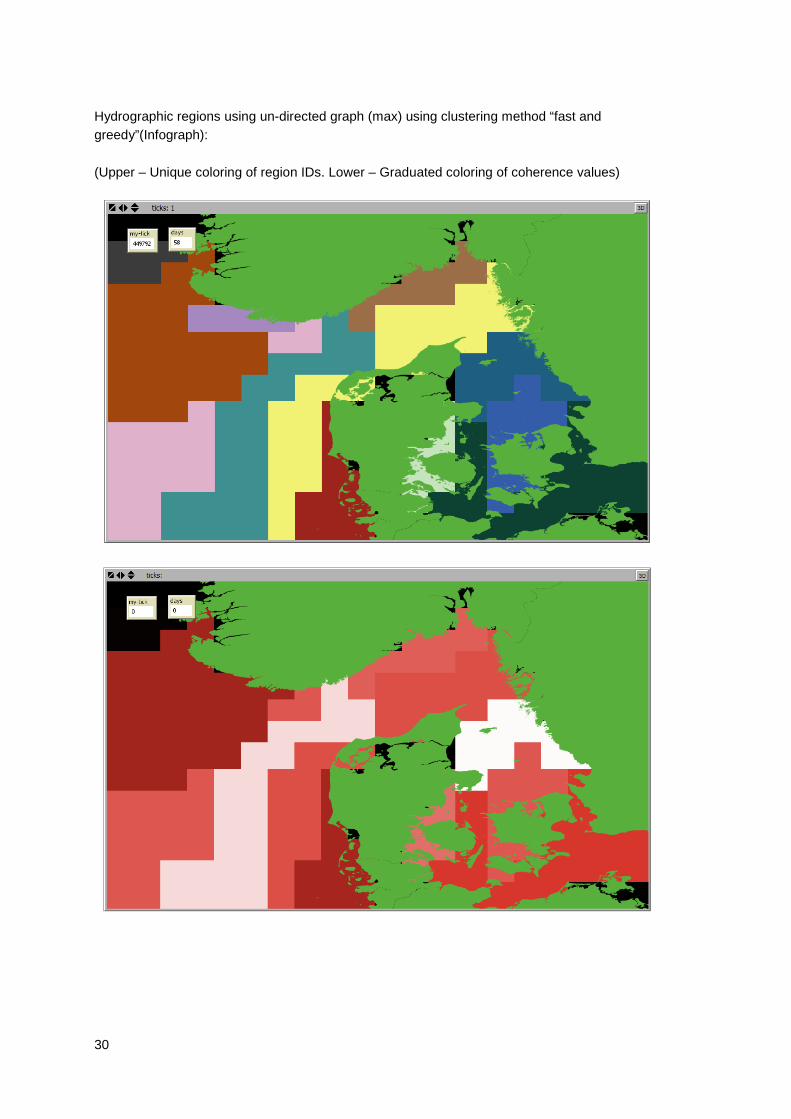
Hydrographic regions using un-directed graph (max) using clustering method “fast and greedy”(Infograph): (Upper – Unique coloring of region IDs. Lower – Graduated coloring of coherence values)

31

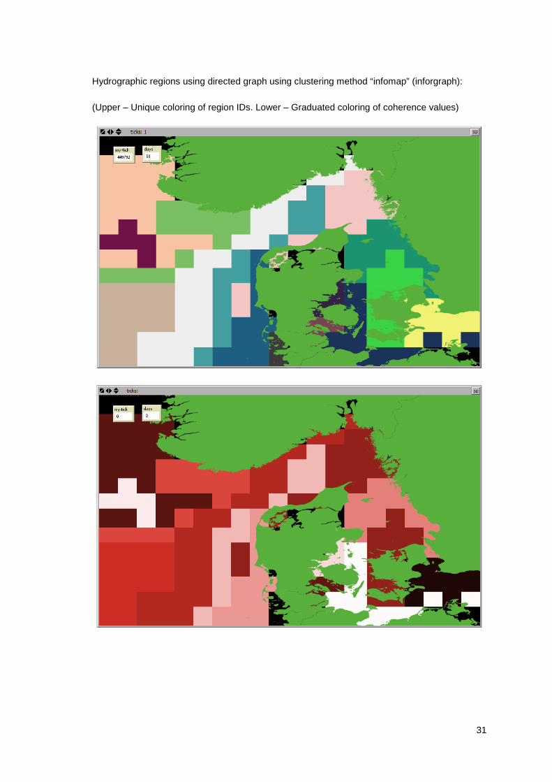
Hydrographic regions using directed graph using clustering method “infomap” (inforgraph): (Upper – Unique coloring of region IDs. Lower – Graduated coloring of coherence values)

32

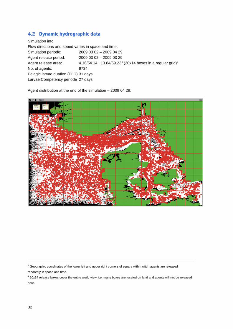
4.2 Dynamic hydrographic data Simulation info Flow directions and speed varies in space and time. Simulation periode: 2009 03 02 – 2009 04 29 Agent release period: 2009 03 02 – 2009 03 29 Agent release area: 4.16/54.14 13.84/59.233 (20x14 boxes in a regular grid)4 No. of agents: 9734 Pelagic larvae duation (PLD) 31 days Larvae Competency periode 27 days Agent distribution at the end of the simulation – 2009 04 29:

3 Geographic coordinates of the lower left and upper right corners of square within witch agents are released

randomly in space and time. 4 20x14 release boxes cover the entire world view, i.e. many boxes are located on land and agents will not be released

here.

33

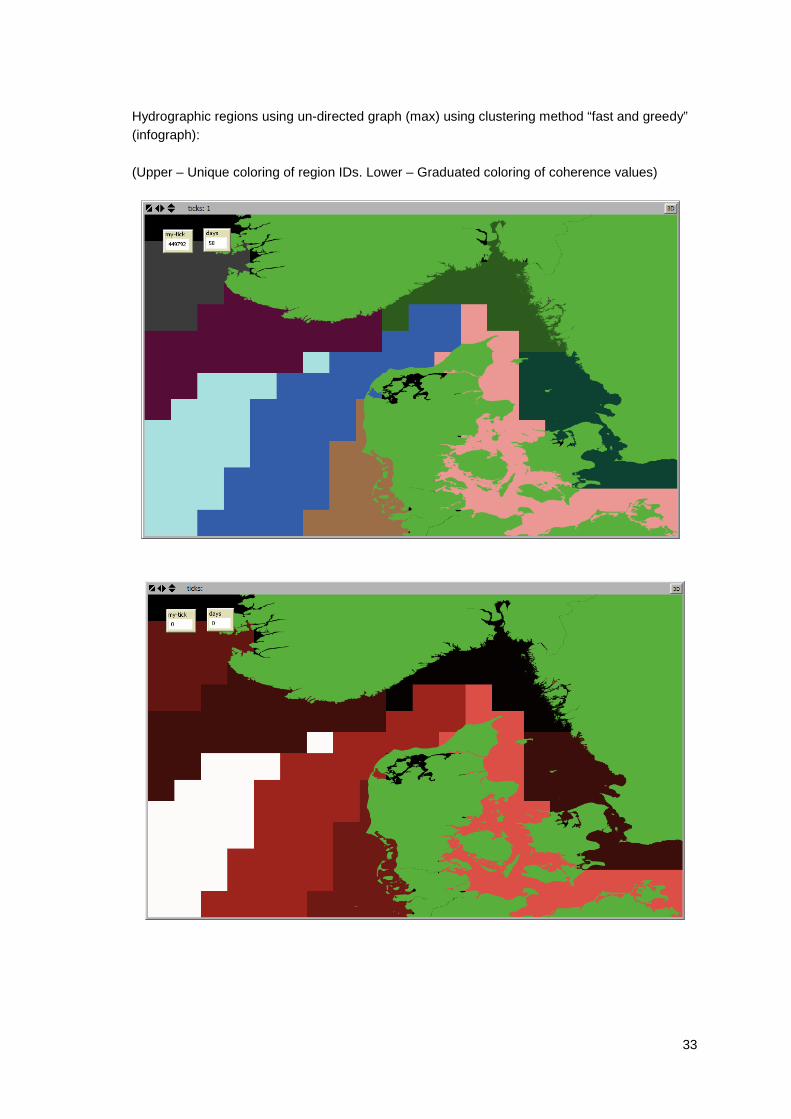
Hydrographic regions using un-directed graph (max) using clustering method “fast and greedy” (infograph): (Upper – Unique coloring of region IDs. Lower – Graduated coloring of coherence values)

34

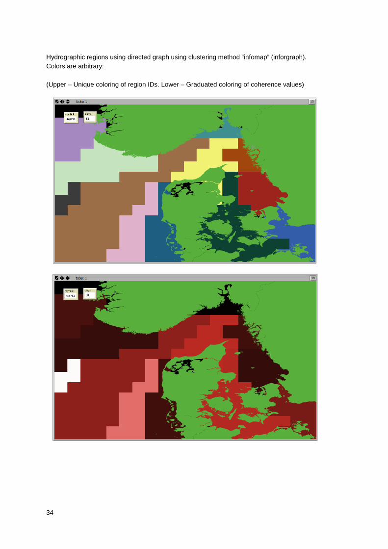
Hydrographic regions using directed graph using clustering method “infomap” (inforgraph). Colors are arbitrary: (Upper – Unique coloring of region IDs. Lower – Graduated coloring of coherence values)

35

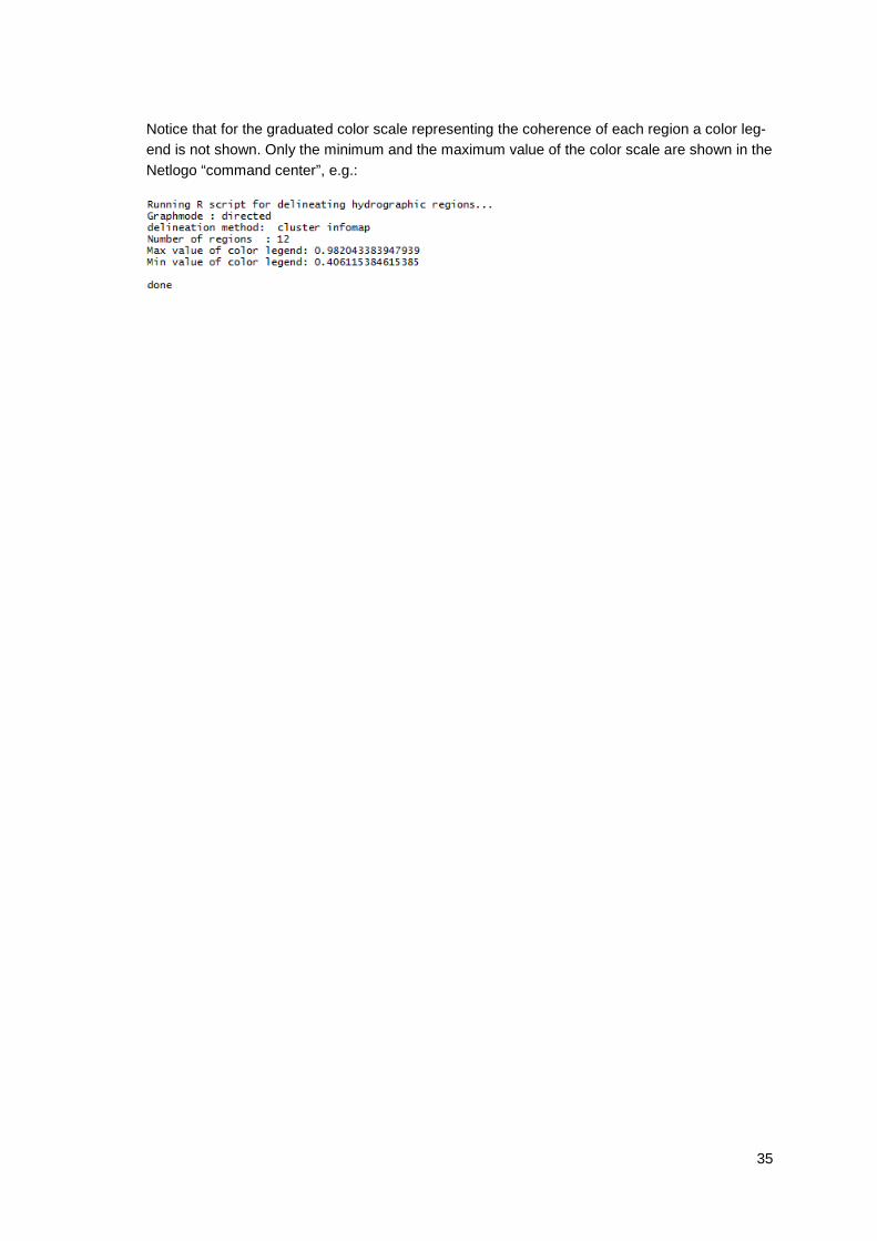
Notice that for the graduated color scale representing the coherence of each region a color leg-end is not shown. Only the minimum and the maximum value of the color scale are shown in the Netlogo “command center”, e.g.:

36

5. Installation guide The installation of the SRAAM tool require as a minimum 3 software components:

- R 3.2.3 for Windows - Netlogo 5.3.1 - IBMLib

Since Netlogo requires JAVA, make sure you have a correct JAVA version installed on your pc.

5.1 R installation

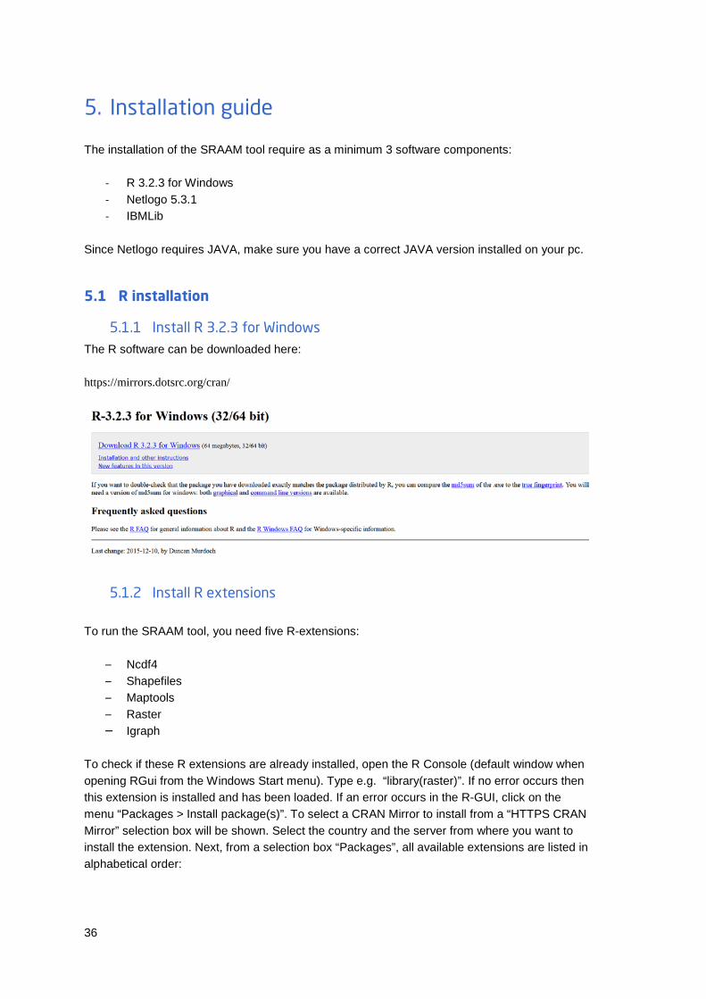
5.1.1 Install R 3.2.3 for Windows The R software can be downloaded here: https://mirrors.dotsrc.org/cran/

5.1.2 Install R extensions To run the SRAAM tool, you need five R-extensions:

– Ncdf4 – Shapefiles – Maptools – Raster – Igraph

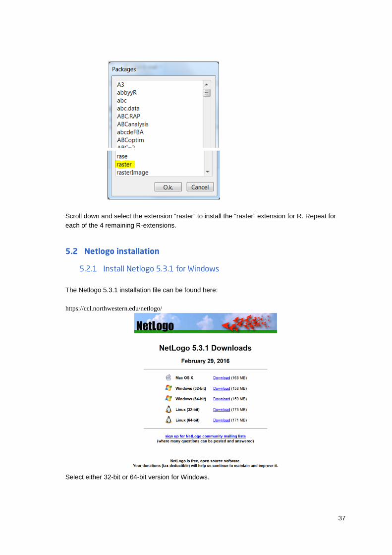
To check if these R extensions are already installed, open the R Console (default window when opening RGui from the Windows Start menu). Type e.g. “library(raster)”. If no error occurs then this extension is installed and has been loaded. If an error occurs in the R-GUI, click on the menu “Packages > Install package(s)”. To select a CRAN Mirror to install from a “HTTPS CRAN Mirror” selection box will be shown. Select the country and the server from where you want to install the extension. Next, from a selection box “Packages”, all available extensions are listed in alphabetical order:

37

Scroll down and select the extension “raster” to install the “raster” extension for R. Repeat for each of the 4 remaining R-extensions.

5.2 Netlogo installation

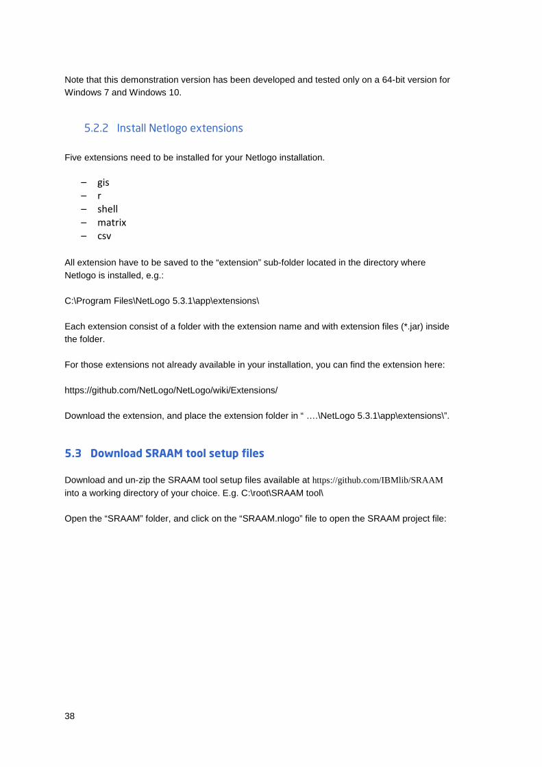
5.2.1 Install Netlogo 5.3.1 for Windows The Netlogo 5.3.1 installation file can be found here: https://ccl.northwestern.edu/netlogo/

Select either 32-bit or 64-bit version for Windows.

38

Note that this demonstration version has been developed and tested only on a 64-bit version for Windows 7 and Windows 10.

5.2.2 Install Netlogo extensions Five extensions need to be installed for your Netlogo installation.

– gis – r – shell – matrix – csv

All extension have to be saved to the “extension” sub-folder located in the directory where Netlogo is installed, e.g.: C:\Program Files\NetLogo 5.3.1\app\extensions\ Each extension consist of a folder with the extension name and with extension files (*.jar) inside the folder. For those extensions not already available in your installation, you can find the extension here: https://github.com/NetLogo/NetLogo/wiki/Extensions/ Download the extension, and place the extension folder in “ ….\NetLogo 5.3.1\app\extensions\”. 5.3 Download SRAAM tool setup files Download and un-zip the SRAAM tool setup files available at https://github.com/IBMlib/SRAAM into a working directory of your choice. E.g. C:\root\SRAAM tool\ Open the “SRAAM” folder, and click on the “SRAAM.nlogo” file to open the SRAAM project file:

39

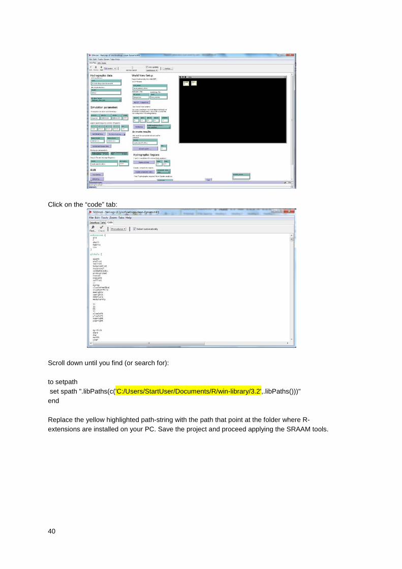
5.4 Setting the path for R-extensions in netlogo Depending on where you have installed the R-extensions (see 5.1.2), you need to set the path in Netlogo before the SRAAM tool will function correctly. Otherwise you will get the error:

In the SRAAM folder, - click on the SRAAM.nlogo file to open Netlogo:

40

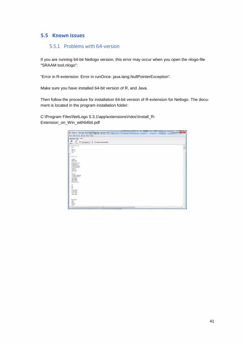
Click on the “code” tab:

Scroll down until you find (or search for): to setpath set spath ".libPaths(c('C:/Users/StartUser/Documents/R/win-library/3.2',.libPaths()))" end Replace the yellow highlighted path-string with the path that point at the folder where R-extensions are installed on your PC. Save the project and proceed applying the SRAAM tools.

41

5.5 Known issues

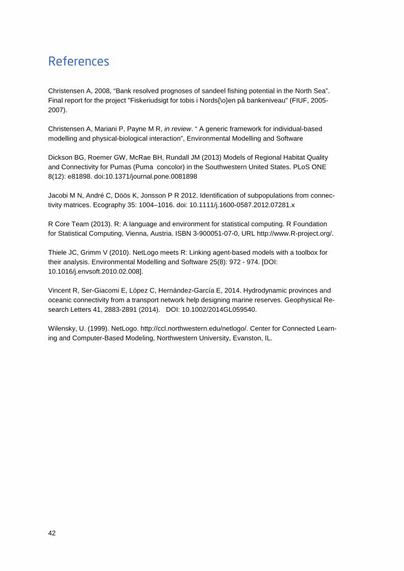
5.5.1 Problems with 64-version If you are running 64-bit Netlogo version, this error may occur when you open the nlogo-file “SRAAM tool.nlogo”: “Error in R-extension: Error in runOnce: java.lang.NullPointerException”. Make sure you have installed 64-bit version of R, and Java. Then follow the procedure for installation 64-bit version of R-extension for Netlogo. The docu-ment is located in the program installation folder: C:\Program Files\NetLogo 5.3.1\app\extensions\r\doc\Install_R-Extension_on_Win_with64bit.pdf

42

References

Christensen A, 2008, “Bank resolved prognoses of sandeel fishing potential in the North Sea”. Final report for the project "Fiskeriudsigt for tobis i Nords{\o}en på bankeniveau" (FIUF, 2005-2007). Christensen A, Mariani P, Payne M R, in review. “ A generic framework for individual-based modelling and physical-biological interaction”, Environmental Modelling and Software Dickson BG, Roemer GW, McRae BH, Rundall JM (2013) Models of Regional Habitat Quality and Connectivity for Pumas (Puma concolor) in the Southwestern United States. PLoS ONE 8(12): e81898. doi:10.1371/journal.pone.0081898 Jacobi M N, André C, Döös K, Jonsson P R 2012. Identification of subpopulations from connec-tivity matrices. Ecography 35: 1004–1016. doi: 10.1111/j.1600-0587.2012.07281.x R Core Team (2013). R: A language and environment for statistical computing. R Foundation for Statistical Computing, Vienna, Austria. ISBN 3-900051-07-0, URL http://www.R-project.org/. Thiele JC, Grimm V (2010). NetLogo meets R: Linking agent-based models with a toolbox for their analysis. Environmental Modelling and Software 25(8): 972 - 974. [DOI: 10.1016/j.envsoft.2010.02.008]. Vincent R, Ser-Giacomi E, López C, Hernández-García E, 2014. Hydrodynamic provinces and oceanic connectivity from a transport network help designing marine reserves. Geophysical Re-search Letters 41, 2883-2891 (2014). DOI: 10.1002/2014GL059540. Wilensky, U. (1999). NetLogo. http://ccl.northwestern.edu/netlogo/. Center for Connected Learn-ing and Computer-Based Modeling, Northwestern University, Evanston, IL.

DTU Aqua

National Institute of Aquatic Resources

Technical University of Denmark

Jægersborg Allé 1

2920 Charlottenlund

Denmark

Tel: + 45 35 88 33 00

aqua@aqua.dtu.dk

www.aqua.dtu.dk