0

WP/17/3

SAMA Working Paper

Commercial Bank Credit and Sectoral Economic Growth:

Granger Causality Analysis

November 2017

By

Saudi Arabian Monetary Authority

Ahmed Alabbadi

Economic Research Department

The views expressed are those of the author(s) and do not necessarily reflect the

position of the Saudi Arabian Monetary Authority (SAMA) and its policies. This

Working Paper should not be reported as representing the views of SAMA.

1

Commercial Bank Credit and Sectoral Economic Growth: Granger

Causality Analysis*

Abstract

This paper examines the long-run relationship between bank credit and economic

growth across the sectors in the Saudi economy using panel data from 1970 to 2014.

The analysis was carried out using panel co-integration and causality techniques

controlling for the presence of cross-sectional dependence. The variables are determined

to be panel I(1) and co-integrated . A uni-causal link from economic growth to bank

credit can be deduced from Panel Granger causality tests. While further examination of

long-run dynamics reveals a narrow causal link from bank credit to economic growth in

the commerce sector, the results have been related to the literature and followed by

policy recommendations.

Keywords: Bank credit, Tradable sectors, Economic growth, financial development, Panel

co-integration.

JEL Classifications: G10, G11, G12, G18, G20.

* The author would like to thank Dr. Os. Ouattara for valuable comments and suggestions. Author contacts:

Ahmed Alabbadi, Economic Research Department, Saudi Arabian Monetary Authority, P. O. Box 2992 Riyadh

11169, Email: aalabadi@sama.gov.sa.

2

1. Introduction

An extensive literature has identified financial sector development as a critical factor in

inclusive economic development. Nevertheless, many empirical studies on the finance-growth

nexus show ambiguous results. These conflicting results could primarily be due to the wide

array of methodologies and datasets used as well as the peculiarities of the cases. While some

studies focus on the case of one economy using either time series or micro-level panel data

methodologies, others use panel data methodologies by pooling data across countries. In many

studies, however, countries with oil-based economies are usually excluded; some justify this

exclusion by suggesting the different factors that generate economic development in these

economies, or pointing out that financial sectors play different roles and have different

structures (Beck, 2010). Therefore, exploring the role of the financial sector development in

economic growth of an oil-based economy such as Saudi Arabia is important for policymakers.

One chief objective of the economic policymaker in Saudi Arabia is to diversify the economy

away from oil dominance. Financial sector development could help in this respect by facilitating

funds for industries that are most reliant on external finance along with small enterprises that

are more opaque and have been freshly introduced in the economy (Beck and Demirgüç-Kunt,

2009; Rajan and Zingales, 1998). These aspects on the relationship between finance and growth

in an oil-driven economy contribute to the importance of this study in addition to the following

point. This is the first empirical study on the finance-growth nexus to employ panel data

methods within the context of one country’s macroeconomic level. This study applies the

analysis on the level of economic sectors; namely, GDP per sector. These different sectors under

analysis are presented in Table (1). Finding the direction of causality is relevant because

determining the causal pattern between financial indicators and the macro-economy has

important implications for policymakers. As it is elsewhere, in theory and in empirical evidence,

there is no consensus on the direction of causality between financial development and economic

growth.

This study addresses the empirical relationship between financial development, namely private

credit, and economic growth for eight sectors of the overall private non-oil sector in Saudi

Arabia. The study covers the period 1970 – 2014 and is organized as follows: Section 2 initiates

3

a general literature review, section 3 presents a brief review of the different econometric

techniques employed, section 4 discusses the empirical results and section 5 provides relevant

policy recommendations after a concise summary.

Table 1: Sector’s description Sector Description

Agriculture Agriculture, fisheries, forestry

Transport Communication and transport

Commerce Wholesale and retail trade

Utility Electricity, water and gas

Mining Non-oil mining and quarrying

Manufacturing Non-oil manufacturing and processing

Construction Building and construction

Services Aggregation of finance sectors and ‘Community, Social & Personal

Services’ to align with bank credit data

Source: SAMA annual report 2015.

2. Brief Literature Review

The finance-growth nexus has been extensively analyzed over the last two decades from aspects

of both financial intermediation and financial markets. Both theoretical and empirical works

remain contested over the channels and even the direction of causality. Generally, the literature

distinguishes a number of main themes for this relationship. This was pioneered by Patrick

(1966)1 who suggested that causality runs in a two-way direction between financial

development and economic growth. At early stages of development, the direction was from

finance to economic growth. Then, as the economy matures, the direction has become from

economic growth to finance. Existing studies report four possible causal patterns in the finance-

growth nexus: finance-led growth or “supply-leading” (where financial development causes

economic growth), growth-driven finance or “demand-following” (where growth exerts a

causal effect on financial development) and the two-way (bi-directional) causal relationship

which is termed feedback. Lastly, few studies have reported no evident causal link in the

finance-growth nexus.

1 - In 1966, based on lessons from the Japanese industrialization experience, Hugh Patrick introduced his theory

on "supply-leading" and “demand-following” causality patterns.

4

In the context of Saudi Arabia, Al-Jasser (1986) studied the role of financial development in

economic development during the period from 1965 to 1984, using financial ratios such as

currency and monetary ratios. The non-oil private sector GDP was used as a proxy for economic

development. He applied both a simple correlation test and a bivariate Granger-Sims causality

test. The result showed that financial development in Saudi Arabia was positively correlated

with economic development. In addition, the results of the causality test revealed that the

causality is unidirectional from the financial development to economic growth as measured by

the non-oil private sector GDP. More recently, Abu Bader and Abu-Qarn (2008a) examined the

causal pattern for six Middle Eastern and North African countries1 within a quadvariate vector

autoregressive framework. Empirically, they used the augmented vector autoregression (VAR)

of Toda and Yamamoto (1995) to test for Granger causality. Their causality testing results

strongly supported the hypothesis that financial development leads to economic growth in the

long run in five out of the six countries tested. Habibullah and Eng (2006) pooled a sample of

Asian developing countries2 and employed the GMM-system technique developed by Arellano

and Bover (1995). They conducted causality testing analysis and used the ratio of domestic

credit to GDP to proxy for financial development and real per capita GDP to proxy for growth.

Their findings supported the contention made by Calderon and Liu (2003) that “there is strong

evidence for the supply-leading growth hypothesis which asserts that financial intermediation

promotes economic growth”. They also observed that liberalization and reform policies have

shown to improve economic growth.

The view that rampant economic growth creates a demand for more financial services which

stimulate the development of the financial sector is dubbed “Growth-driven” or “demand-

following” in the literature. In contrast to the finance-led growth hypothesis, the growth-driven

finance hypothesis suggests that an increase in growth and expansion in the real sector generally

leads to an increased demand for financial services; hence, financial development. This view

was pioneered by Robinson (1952) and Patrick’s (1966) hypothesis of ‘demand-following’,

stipulating that financial development primarily follows the expansion in the economy’s

growth, as a result of an increased demand for financial services.

2- These are Algeria, Egypt, Israel, Morocco, Syria, and Tunisia.

5

Considerable empirical evidence suggests economic growth precedes subsequent financial

development such as the works by Thornton (1996), Waqabaca, (2004), Habibullah (1999),

Ram (1999), and Odhiambo (2010) amongst others. In the same vein, Kuznets (1955), Lucas

(1988), and Levine and Zervos (1996) argued that financial systems do not promote economic

growth. Rather, they respond to the expansion in the real economy.

More recently, Ang and McKibbin (2007) conducted multivariate co-integration and several

causality tests in the small open economy of Malaysia. Their findings suggested that output

growth causes financial development in the long run. Although the country has more features

of a bank-based financial system, the findings did not specify that this form of system has a

significant contribution to growth in the long run. Boulila and Trabelsi (2004)3 studied 16 of

the MENA countries with 25 annual observations for each. They utilized co-integration

techniques based on bivariate VAR in addition to Granger causality. Their findings suggested

that there is little evidence that finance is predicting long-run growth in the sample. Moreover,

empirical evidence confirms that there is a unidirectional causality running from growth in the

real sector to the financial sector.

Al-Yousif (2002) examined 30 developing countries4 for the period 1970-1999 using both time

series and panel data and utilizing Granger’s causality test in an ECM, and Johansen-Juselius

approach to test co-integration . The empirical findings lent strong support to the hypothesis

that there is a feedback causality pattern between financial development and economic growth;

that is, causality is bi-directional. To a lesser extent, however, there is some support for other

directions of causality, supply-leading, demand-leading and no causal relationship. He

concluded that the results are variable-sensitive tending to vary across countries depending on

the kind of variable used to measure financial development as it is in other studies (see for

example, Darrat, 1999; Demetrides and Hussein, 1996).

Chuah and Thai (2004) examined the relationship between financial development and economic

growth in the GCC countries utilizing Bivariate time series for the period 1973–2002. The

empirical evidence indicated that there is a bidirectional causal link between financial

3- They studied Algeria, Bahrain, Egypt, Iran, Jordan, Kuwait, Mauritania, Morocco, Oman, Qatar, Saudi

Arabia, Sudan, Syria, Tunisia, Turkey, and the UAE for time-series sets ranging from 1960 to 2002. 4- This includes the GCC countries: Saudi Arabia, Kuwait, Bahrain, Oman, Qatar, and the UAE.

6

development and economic growth in five out of the six GCC countries, with the exception of

Kuwait where causality runs from finance to growth.

Similarly, Al-Awad and Harb (2005) examined the causal pattern in Middle Eastern countries5.

Empirically, they combined both panel co-integration techniques along with the conventional

time series methodologies such as Johansen’s method, Granger causality and variance

decompositions. Overall, findings from panel co-integration tests suggested a long-term relation

between financial development and economic growth. Furthermore, there was evidence of a

unidirectional causal pattern from economic growth to financial development and no feedback

causality. They also applied causality tests based on individual countries’ time series but the

evidence on the direction of causation was inconclusive.

Within the context of the Saudi economy, Almalki (2011) examined the causal and dynamic

relationship between financial intermediary development and economic growth using time

series data over the period from 1970 to 2008. He employed the ARDL-bounds testing approach

to co-integration proposed by Pesaran et al. (2001). Causality results support the bidirectional,

supply-leading and the demand-following hypotheses in terms of the relationship between

financial development (banking sector), human capital, openness and economic output in Saudi

Arabia.

Focusing also on Saudi Arabia, Samargandi et al. (2014) studied the link between various

elements of financial development, including bank credit, on one side and oil- and non-oil GDP

on the other. They based their time series analysis on ARDL framework covering 42 years span.

Their generalized results (using composite index to gauge financial development) suggested the

non-oil sector is favorably affected by financial development at 10% significant level and a

magnitude that “does not warrant a positive relationship” with the economy as a whole.

Finally, there were also studies that suggested evidence cannot be discerned on the causal

relationship between financial development and economic growth. This was a view held by

Lucas (1988) who stated, “Economists badly overstress the role of financial factors in economic

growth”. Similar views reemerged as recently as Arestis (2005) who found no evidence to

support the view that financial development helps in predicting future economic growth if all

5- These are Algeria, Egypt, Iran, Jordan, Kuwait, Morocco, Saudi Arabia, Syria, Tunisia, and Turkey over the

period 1969-2000.

7

contemporaneous correlations in the relationship are accounted for. Furthermore, Levine et al.

(1999) posited that the causality pattern depends on the level of economic development. In less

developed countries, financial development causes economic growth, and vice versa in

developed countries.

3. Methodology

In this study, the empirical modelling framework consists of four steps. First, the study will

establish the order of integration for the variables. Secondly, analysis of potential co-integrated

relationship follows using different tests. Thirdly, causality tests suitable for the dataset will be

implemented. These methodologies are described and justified in a concise manner in the

following lines.

According to the standard co-integration literature, the concept of co-integration was first

introduced by Granger (1969), which basically conveys the presence of a long-run relationship

between variables in one model. Testing for co-integration is to test whether two or more

integrated variables deviate significantly from a certain relationship (Abadir et al., 1999). One

can say variables are co-integrated if they maintain predictable co-movement over time. This

means short-term disturbances will be corrected in the long run. If not co-integrated in the long

run, two series may wander arbitrarily far away from each other over time (Dickey et. al., 1991).

That is, if a linear combination of the integrated variables of order d is integrated of a

smaller order than d, then these variables are co-integrated . This can be tested after

establishing the order of integration for the series. Once co-integration is established, the long-

run parameters can be estimated efficiently using panel techniques not principally different from

methodologies applied to single time-series models. The use of panel data contributes to the

power of co-integration analysis, allowing the estimation of better parameters than would have

been identified along the time or with the cross-sectional dimensions alone. However, the

increased power is usually achieved under assumptions of parameter homogeneity and error

cross- section independence in the case of linear panel data models with a short time dimension

(Geweke et al., 2006). Pierse and Snell (1995) as well as Perron (1991) found that the power of

standard Dickey-Fuller (DF) and Augmented Dickey-Fuller (ADF) unit root tests can be

improved if the time dimension is extended. With a longer time span, Pedroni (2004) also

established that the time span of the data more than the frequency is important for increasing

the power of the tests. Nevertheless, an extended time series that covers long period can suffer

8

other types of problems, such as structural breaks and regime shifts. One way to maintain

increased power of the tests and the number of observations can be by means of compiling

cross-sectional data, say, across countries, sectors, industries, etc., which leads to better

performance of panel data unit root and co-integration tests.

3.1 Unit Root Testing

Before testing for the existence of a long-run relationship, it is necessary to determine the level

of integration for the variables and test for the existence of unit roots in the panel-series. Using

co-integration techniques requires that the study must first check the properties of the

underlying series. Taking the autoregressive property of the time-series data in mind, the level

of integration of each variable must first be established before the regression relationship can

be estimated between the variables. Many tests have been developed to check for the presence

of a unit root in a series. This study applied panel unit root tests with cautious consideration of

the choice of tests so as to be suitable to the nature of the study’s panel dataset (such as

homogeneity and the presence of cross-sectional dependence). Hence, a number of panel data

unit root tests that account for cross-sectional dependence will be employed. Due to Breitung

(2000), a new test is proposed that highly resembles the ADF regression as in LLC test assuming

a common unit root. An alternative panel unit root test advanced in Hadri (2000) proposed the

reversed hypothesis by assuming that the panel data have a common stationary process while

an alternative hypothesis assumes that the panel is of nonstationary process. Recently, also

studies attempting to account for the presence of cross-sectional dependence in unit root tests

include Pesaran (2004) who suggested a simpler way of “getting rid of cross-sectional

dependence, based on augmenting the usual ADF regression with the lagged cross-sectional

mean and its first difference to capture the cross-sectional dependence that arises through a

single factor model” (Baltagi, 2013).

3.2 Co-integration Tests

Co-integration came out of the attempt to realize potentially long-run relationships between

variables. As compared to the well-established panel unit root tests, the analysis of co-

integration in panels is a relatively new area of exploration.6 This field was pioneered by the

research of Kao (1999), McCoskey and Kao (1998), and Pedroni (1999). Since then, panel co-

6 - Surveys of the panel unit root and cointegration literature are covered in Banerjee (1999), Baltagi and Kao

(2000), Choi (2006), and Breitung and Pesaran (2006).

9

integration tests have become widely used in the finance-growth nexus study.

The study’s primary objective is to test whether there is a long-run co-integrating

relationship between economic growth and financial development variables. To this end,

the study employed Kao’s (1999) residual-based panel co-integration test. After which, the

study applied the tests due to Larsson et al. (2001), called Maximum-Likelihood-

Based Tests. To add to robustness, the tests developed by Westerlund (2007) and

described as ECM-based Panel Co-integration Tests will also be used along with further

variation of the tests developed by Westerlund and Edgerton (2007a).

3.3 Causality Analysis

After establishing that a co-integrated relationship between financial development and

economic growth exists, the study proceeded to also test for Granger causality as introduced by

Engle and Granger (1987). The essential advantage of this method is to establish the role

financial development plays in the economic process, whether it is supply-leading or demand-

following. Granger causality assumes a temporal structure in order to address the question of

causal direction using purely probabilistic methods. Granger (1969) provided a method for

testing temporal causality that was met with wide approval and was subsequently developed to

application on panel data sets.

Kidd et al., (2006) suggested that failure to analyze the presence of heterogeneity in cross-

section units could easily lead to faulty conclusions such as finding a causal link in all the cross-

section units when it only exists in a subset of the examined units. This could even lead to

rejecting the link of the causal link for all the cross-section units when it only exists in at least

a subset of the cross-section units (Kidd et al., 2006). Kar et al. (2011) identified three

approaches to causality in panel time-series. An approach was developed by Hurlin and Venet

(2001, 2003) and Hurlin (2004, 2007, 2008) and is based on the Panel Granger causality.

For two variables X and Y, Hurlin and Venet (2003) represented a VAR model framework in a

panel data with fixed effects as follows:

𝑋𝑖,𝑡 = ∑ 𝑎𝑘𝑋𝑖,𝑡−𝑘 + ∑ 𝐵𝑖𝑘𝑌𝑖,𝑡−𝑘 + 𝑣𝑖,𝑡

𝑝

𝑘=𝑜

𝑝

𝑘=1

(29)

10

𝑌𝑖,𝑡 = ∑ 𝛾𝑘𝑋𝑖,𝑡−𝑘 + ∑ ∅𝑖𝑘𝑋𝑖,𝑡−𝑘 + 𝑣𝑖,𝑡

𝑝

𝑘=𝑜

𝑝

𝑘=1

(30)

where 𝑣𝑖,𝑡 = 𝜏𝑖 + 𝜀𝑖,𝑡 , 𝜏𝑖 are the individual effects and 𝜀𝑖,𝑡 are the disturbance terms and are

i.i.d. (0, 𝜎𝜀2).

If the homogenous causality hypothesis is rejected7, the study proceeded to test for panel

causality between the variables X and Y. This means that causality may exist in some of the

cross-sections and implies testing in which of the N individuals of the panel the causality exists.

Hurlin and Venet (2003) is proposed here to use a conventional Granger-causality test for each

cross-sectional unit of the panel. But since, most of the time, macroeconomic variables are non-

stationary and co-integrated , the study opted for the method developed by Pesaran et al. (1999)

which was more suitable in estimating non-stationary heterogeneous panels. The method is

called the Pooled Mean Group (PMG) and is basically a dynamic error-correction model that

allows the short-run parameters to vary across the cross-sections (countries) while at the same

time imposes restriction on long-run elasticities to be identical. In Pesaran et al. (1999), an

alternative technique called the Mean Group (MG) estimator was also presented. It simply

involves the estimation of separate equations for each cross-section and the computation of the

mean of the estimates. This is carried out without imposing any constraint on the parameters.

Choosing between PMG and MG is based on the test of the homogeneity of the long-run

coefficients. This test is known as Hausman test and is based on the null that the two sets of

coefficients generated by the PMG and MG estimators are not statistically different (Mahony

and Vecchi, 2003). For causality to hold, it has to be negative and significant for the error

correction model to be valid. Yet again, the presence of cross-sectional dependence must be

accounted for. Kar et al. (2011) suggested that if cross-sectional dependency and country

specific heterogeneity in a panel causality analysis are ignored, it could form potential sources

of misleading inferences about the strength and type of causality.

7- In our sample, cross-sector heterogeneity may arise from different factors, such as the degree of credit reliance

on sectors as documented in (Rajan and Zingales 1998).

11

4. Empirical Analysis

4.1 Data and variables

To investigate the relationship between growth and financial development, this study applied a

balanced panel for the eight sectors over the period 1970-2014 and estimated the following

baseline specification:

𝑌𝑖𝑡 = 𝐵0𝑖 + 𝐵1𝑖𝐶𝑅𝐸𝑖𝑡 + 𝜀𝑖𝑡 (34)

where Y is the real GDP per sector, CRE is the proxy of financial development which is the

ratio of bank credit to a particular sector of GDP, i and t represent sector and time period,

respectively, and 𝜀 is an error term. This model will be used for the period of economic

development in Saudi Arabia from 1970-2014 for eight economic sectors. Once the researcher

confirms the presence of a co-integrating relationship among the variables, it is possible then to

proceed to examine the causal link between the variables.

Since this empirical analysis deals with GDP per sector, the study took the natural log of a GDP

per sector as the dependent variable drawn from SAMA’s Annual Report (2015). It can be

argued that the GDP as a whole in the case of oil-driven economies does not perfectly measure

the level of economic activity. This is because of the influence of oil production levels and its

prices being determined outside of the economy.

On the other hand, theory suggests that commercial credit provided to the private sector, one

aspect of financial development, translates into higher productivity to a much larger extent than

credit provided to the public sector. The literature also distinguishes bank credit to the private

sector as a channel for quality investments because of the financial intermediaries’ evaluation

of project viability from loans directed at the public sector (Beck et al., 2000). This measure is

popular in the literature and was employed by studies such as Ang and McKibbin (2007), Levine

et al. (2000), Odhiambo (2007), and others. Higher levels of this ratio are indicative of higher

levels of financial intermediaries’ engagement with private sector and lower transaction costs.

For the purpose of this study, the standard measure for bank credit used is in line with relevant

literature, which is private credit for the sector as a ratio to real GDP of the respective sector.

The data employed were in real terms and obtained from SAMA’s Annual Report (2015).

12

4.2 Unit Root Results

To pool the cross-sectional data and conform to the panel methodologies, the Breitung (2000),

Hadri (2000), Harris and Tzavalis (1999), and Pesaran (2005) panel unit root tests were applied

to the cross-sectional data. Cross-sectional dependence tests were employed: Friedman (1937)

and Frees (1995, 2004) are semi-parametric tests in addition to the parametric testing

procedures proposed by Pesaran (2004). In addition, the Breusch and Pagan (1980) (B-PLM

henceforth) test was used which is a more appropriate test for panels with a large T and a small

N. These tests are valid in fixed-effects or random-effects panel data models with the standard

assumption in panel data models that the error terms are independent across cross-sections. The

tests (Table 5.2) show a rejection of the null hypothesis of cross-sectional independence which

indicates the presence of cross-sectional dependence in the panel set.

Table 2: Tests of Cross-Sectional Dependence

Friedman test B-PLM test Frees test Pesaran test

Stat P-val Stat P-val Stat Stat P-val

45.62***

0.00 267.35*** 0.00 2.601*** 5.09*** 0.00

The null hypothesis of all the tests is the presence of cross-sectional independence. (***), (**), and (*)

denote the rejection of the null hypothesis at 1%, 5%, and 10% respectively. B-PLM denotes the Breusch

Pagan test. Test was performed in STATA software.

Cross-sectional dependence is evident (Table 2) when tested across sections, which requires

implementing unit-root tests with special specifications (options) to subtract cross-sectional

means or allow for cross-sectional dependence. The first generation panel unit root tests (i.e.

Levin et al., (2002)) allowed for parameter heterogeneity but assumed errors were cross-

sectionally independent and thus were not adopted here. More flexibility in underlying the

assumptions came with the tests by Moon and Perron (2004) and Pesaran (2007) which allowed

for error cross-section dependence. Pesaran’s (2003) test (CADF) runs the t-test for unit roots

in heterogenous panels with cross-section dependence parallel to Im, Pesaran and Shin (IPS,

2003). As alluded to, the tests are based on the mean of individual DF (or ADF) t-statistics of

each unit in the data time-series data set. To eliminate problems arising from cross dependence,

the standard DF (or ADF) regressions are “augmented” with the cross section averages of

lagged levels and first-differences of the individual series (as in CADF statistics). The unit root

tests for the Hadri , Harris-Tzavalis, and Breitung tests are provided in Table (3), and the test

13

for Pesaran’s (2003) test (CADF) is provided in Table (4). Results confirm that the variables of

interest are I(1) and therefore can proceed to test for the presence of a co-integrated

relationship.

Table 3: Panel Unit Roots Tests

Hadri Harris-

Tzavalis

Breitung

Levels Diff Levels Diff Levels Diff

GDP 39.3** 22.63** -0.30 -24.5** 1.57 -5.09**

CRE 15.9** 1.05 -0.03 -25.11** -0.10 -8.23**

Note: In the null hypothesis for the Hadri test, there is no unit root while for the Harris-Tzavalis and Breitung

tests, there is a unit root. Tests are carried for constant and trend. The specification used for the Hadri test is

demean, and for the Breitung and Harris-Tzavalis tests, they are robust as prescribed in the presence of cross-

sectional dependence. (***), (**), and (*) denote the rejection of the null hypothesis at 1%, 5%, and 10%

respectively.

Table 4: CADF Panel Unit Root tests in the Presence of Cross-sectional Dependence

(Pesaran 2005)

Series

GDP

∆GDP

CRE

∆ CRE

Const. Constant & Trend

Z[t-bar] P-Value Z[t-bar] P-Value

-0.037 0.48

-12.61***

0.00

-0.76 0.22

-2.33**

0.01

0.60 0.52

-4.88***

0.00

-0.54 0.29

-1.30* 0.09

Note: Critical values of t-bar are CV1%: -2.380, CV5%: -2.200 and CV10%: -2.380 when the deterministic

term chosen is constant and CV1%: -2.88, CV5%: -2.72 and CV10%: -2.63 when the deterministic terms chosen

are constant & trend. (***), (**), and (*) denote the rejection of the null hypothesis at 1%, 5%, and 10%.

4.3 Co-integration Test Results

Table 5: Kao Residual-based Panel Co-integration Tests

GDP CRE

t- statistic

ADF -2.70(0.00)***

(***) denotes the rejection of the null hypothesis of no co-integration at 1% probability. The test uses automatic

lag length selection based on AIC, with a maximum lag of 4, Newey-West automatic bandwidth selection and

Bartlett Kernel. Test was performed in Eviews software.

Table 6: Westerlund’s (2008) Durbin-Hausman Panel Co-integration Test

Series: GDP CRE

Westerlund’s

Durbain-Hausman

test

DHp 9.82***

DHg 4.53***

The null hypothesis is no co-integration . (***), (**), and (*) denote the rejection of the null hypothesis at 1%,

5%, and 10% respectively. Estimation was performed in GAUSS software.

14

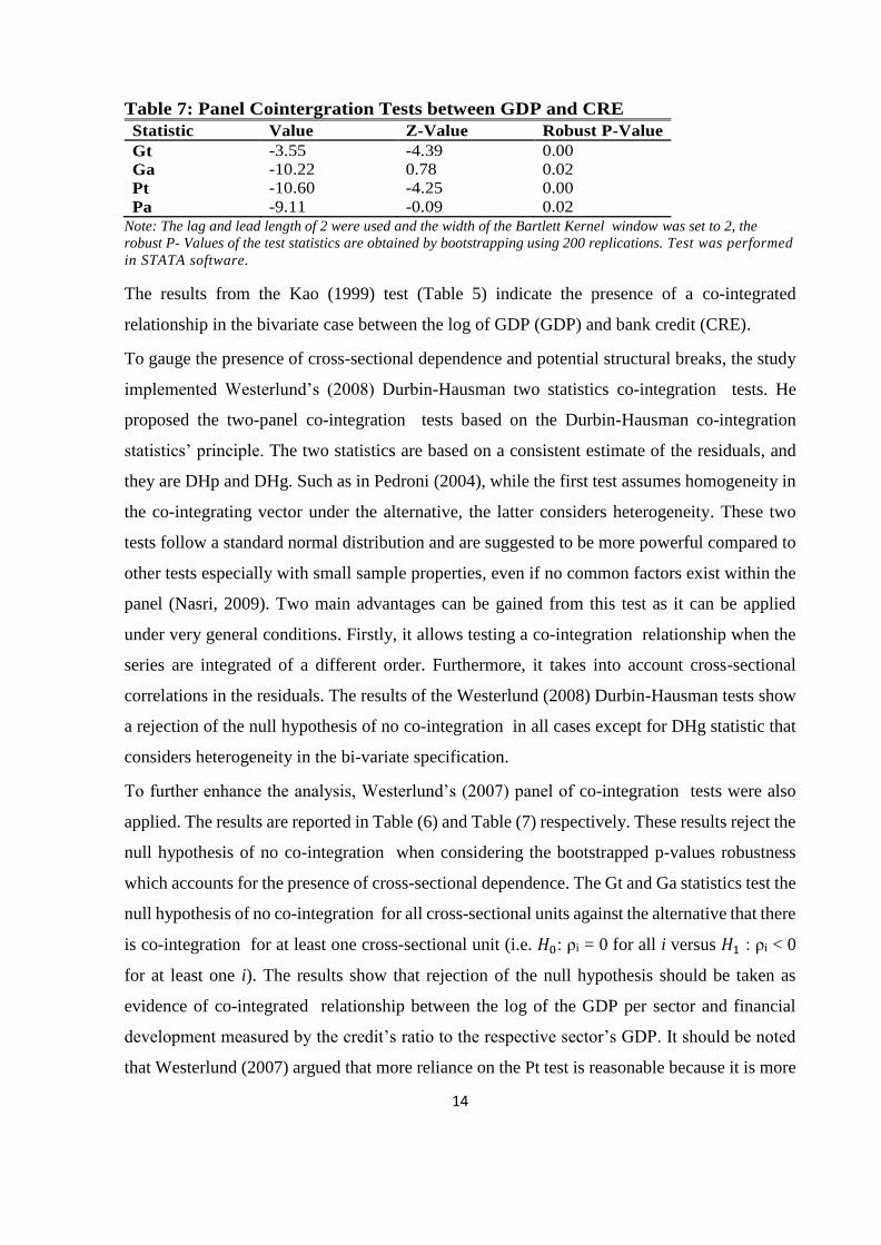
Table 7: Panel Cointergration Tests between GDP and CRE

Statistic Value Z-Value Robust P-Value

Gt -3.55 -4.39 0.00

Ga -10.22 0.78 0.02

Pt -10.60 -4.25 0.00

Pa -9.11 -0.09 0.02

Note: The lag and lead length of 2 were used and the width of the Bartlett Kernel window was set to 2, the

robust P- Values of the test statistics are obtained by bootstrapping using 200 replications. Test was performed

in STATA software.

The results from the Kao (1999) test (Table 5) indicate the presence of a co-integrated

relationship in the bivariate case between the log of GDP (GDP) and bank credit (CRE).

To gauge the presence of cross-sectional dependence and potential structural breaks, the study

implemented Westerlund’s (2008) Durbin-Hausman two statistics co-integration tests. He

proposed the two-panel co-integration tests based on the Durbin-Hausman co-integration

statistics’ principle. The two statistics are based on a consistent estimate of the residuals, and

they are DHp and DHg. Such as in Pedroni (2004), while the first test assumes homogeneity in

the co-integrating vector under the alternative, the latter considers heterogeneity. These two

tests follow a standard normal distribution and are suggested to be more powerful compared to

other tests especially with small sample properties, even if no common factors exist within the

panel (Nasri, 2009). Two main advantages can be gained from this test as it can be applied

under very general conditions. Firstly, it allows testing a co-integration relationship when the

series are integrated of a different order. Furthermore, it takes into account cross-sectional

correlations in the residuals. The results of the Westerlund (2008) Durbin-Hausman tests show

a rejection of the null hypothesis of no co-integration in all cases except for DHg statistic that

considers heterogeneity in the bi-variate specification.

To further enhance the analysis, Westerlund’s (2007) panel of co-integration tests were also

applied. The results are reported in Table (6) and Table (7) respectively. These results reject the

null hypothesis of no co-integration when considering the bootstrapped p-values robustness

which accounts for the presence of cross-sectional dependence. The Gt and Ga statistics test the

null hypothesis of no co-integration for all cross-sectional units against the alternative that there

is co-integration for at least one cross-sectional unit (i.e. 𝐻0: ρi = 0 for all i versus 𝐻1 : ρi < 0

for at least one i). The results show that rejection of the null hypothesis should be taken as

evidence of co-integrated relationship between the log of the GDP per sector and financial

development measured by the credit’s ratio to the respective sector’s GDP. It should be noted

that Westerlund (2007) argued that more reliance on the Pt test is reasonable because it is more

15

robust to cross-sectional correlations if present since the Pa statistic is normalized by T, which

may cause the test statistic to frequently reject the null too. This level of the analysis reveals

that there is a single co-integrating vector. Therefore, it can be concluded that the co-integrated

relationship exists between the variables of interest, and thereby we proceed to examine the

nature of the causal relationship.

4.4 Causality Analysis

Table 9: Pair-wise Granger panel causality test

Direction of

Causality

L = 1 L = 2 L = 3 L=4

CRE → GDP 1.5(0.69) 0.39(0.67) 0.52(0.00) 1.9(0.94)

GDP→CRE 125.5(0.00) *** 0.39(0.67) 0.52(0.66) 18.9(0.00) ***

(***) denotes the rejection of the null hypothesis at 1%. L is lag length, F-statistics are reported with P-values in

parenthesis.

In the Granger pair-wise panel causality test, the null hypothesis states non-existence of causal

relationships across N. If this null is rejected, there is evidence of Granger-causality. The test

results from table (9) show a causal link running from the GDP to the bank credit when tested

with 1, 3, and 4 lags. A causal link from the bank credit to the GDP, on the other hand, could

not be established.

Since the Granger causality hypothesis is rejected as running from bank credit to GDP, we then

proceed to find in which of the cross-sections (sectors) the causal links –if at all – are present.

Given this study utilizes a panel of variables that are found to be co-integrated , it is suitable to

employ an error-correction model in examining the causal link between bank credit and

economic growth. To this end, two methods are commonly employed in non-stationary panels:

the Mean Group (MG) due to Pesaran & Shin (1995) or the Pooled Mean Group (PMG)

estimation of Pesaran et al. (1999). The choice between the two procedures can be

based on the Hausman test. The validity of the long-run homogeneity restriction across

sectors, and hence the efficiency of the PMG estimator over the other estimators, is

examined by the Hausman test. This will test the homogeneity of the long-run coefficients.

The null hypothesis here is that the two sets of coefficients generated by the PMG and MG

estimators are not statistically conflicting. It has been reported that under the null hypothesis

the PMG estimators are consistent and more efficient than the MG estimators (see Pesaran

et al., 1999).

16

Table 10: Hausman Test between PMG and MG

Ho: The difference in coefficients is not systematic

Hausman stat (𝜹𝟐) P value

0.09 0.75

The Hausman test is carried out after running the PMG and MG estimations successively.

Table 11: Panel Causality between CRE and GDP

Sectors L-R causality

(z-stat)

𝜑i =0

Agriculture -0.07(0.94)

Commerce 2.17(0.03)***

Construction 0.55(0.58)

Manufacture 1.53(0.12)

Mining -0.77(0.44)

Services -0.81(0.41)

Transportation

and

Communication

-0.68(0.49)

Utilities 1.29(0.20)

The P-values are in parentheses, and (***), (**), and (*) denote the rejection of the null hypothesis at 1%, 5%,

and 10% respectively.

For MG, however, no constraints are placed on coefficients whether in short- or long-run; the

suitability of either is decided according to the results of the Hausman test as in Table (10). As

for Hausman test results (Table 10), at 10 per cent significance, the null hypothesis of the

homogeneity of the long-run coefficients cannot be rejected. It can be concluded that the PMG

estimators are consistent and more efficient than MG estimators for the purpose of this study’s

estimation. Subsequently, to assess the causality between bank credit and economic growth,

this study opts for the PMG estimation.

The panel causality analysis based on the error correction term obtained from the PMG model

is presented in Table (11). Results indicate that bank credit to the commerce sector shows a

strong causal link to the sector’s GDP. Overall, the panel causality test supports that financial

development, as proxied for by commercial bank credit, follows a ‘demand-following’ pattern

17

in general. The financial development may take place following, and in response to, growing

demand from the real economy and is not a leading factor in economic growth across sectors.

Exception to that exists only in the commerce sector where causality seems to be running from

bank credit to the sector GDP.

5. Conclusion

A simple model was constructed to examine the causal link between bank credit and economic

growth at the sectoral level. The variables were tested for cross-section dependence and found

to exhibit strong cross-sectional dependence. This could be attributed to the interlinked

relationships between the economic sectors in Saudi Arabia and their pronounced exposure to

government spending. Using a novel methodology, panel causality tests, as developed by Hurlin

(2004, 2007, 2008) and Hurlin and Venet (2003), revealed insightful contribution to the

literature. Results from Granger causality tests seem to echo earlier studies that held a general

view of a Saudi banking system following the passive or “demand-following” approach

(Abdeen and Shook, 1984; Johany et al., 1986; Dukheil, 1995). Only in the commerce sector

does the analysis reveal a long-run causal link running from commercial bank credit to the

sector’s GDP. This empirical evidence shows that banks active lending to the commercial

sector, which includes retail, wholesale, and trade outlets, has spurred economic expansion in

the sector as measured by it’s GDP. The evidence can also be in concurrence with Ramady

(2010), who suggests that bank credit to the private sector suffers short-termism, manifested in

the absence of a long-run causal link. This aspect in commercial bank credit activities is

unfavorable to the development of productive tradable sectors which usually require the

commitment of long-term financing. The results stress the notion that the banking sector, while

sufficiently sophisticated, has functions that were not optimized effectively to exert positive

impact on economic growth across productive sectors. For policy makers, this may signal sub-

optimal allocation of credit and an incentive mis-match on the part of the intermediary sector.

The recommendation is to hasten banking sector reforms to align incentives with the national

vision 2030, and induce sophisticated instruments that cater to the financing needs of small and

medium enterprises (SMEs), especially in the tradable sector.

18

Bibilography

Abadir, K. M., Hadri, K. & Tzavalis, E. (1999). “The influence of VAR dimensions on

estimator biases.” Econometrica, 67, 163-181.

Abu-Bader, S. & Abu-Qarn, A. S. (2008a). “Financial development and economic

growth: empirical evidence from six MENA countries.” Review of Development

Economics, 12(4), 803-817.

Abu-Bader, S. & Abu-Qarn, A. S. (2008b). “Financial development and economic

growth: the Egyptian experience.” Journal of Policy Modeling, 30(5), 887-898.

Al-Awad, M. & Harb, N. (2005). “Financial development and economic growth in

the Middle East.” Applied Financial Economics, 15, 1041-1051.

Al-Jasser, M. (1986). The role of financial development in economic development: the

case of Saudi Arabia. Ph. D Dissertation. Riverside, California: University of California.

Almalki, A. M. (2008). “Has the Saudi stock market grown during the period 2003-

2007?” In the Proceedings of the 2 n d Saudi International Innovation Conference.

University of Leeds.

Al-Yousif, Y. K. (2002). “Financial development and economic growth; another look at

the evidence from developing countries.” Review of Financial Economics, 11, 131-

150.

Amsler, C. & Lee, J. (1995). “An LM test for a unit root in the presence of a structural

change.” Econometric Theory, 11(2), 359-368.

Ang, J. B. & McKibbin, W. J. (2007). “Financial liberalization, financial sector

development and growth.” Journal of Development, 84(1), 215-233.

Arellano, M. & Bover, O. (1995). “Another look at the instrumental variable estimation

of error-components models.” Journal of Econometrics, 68(1), 29-51.

Arestis, P. (2005). “Financial liberalization and the relationship between finance and

growth.” CEPP Working Paper No. 05/05. Centre for Economic and Public Policy,

University of Cambridge.

Bai, J. & Ng, S. (2004). “A panic attack on unit roots and co-integration .” Econometrica,

72, 1127-1177.

Baltagi, B. H. (2013). Econometric Analysis of Panel Data. 5th ed. New York: John

Wiley & Sons.

Banerjee, A., Dolado, J. & Mestre, R. (1998). “Error-correction Mechanism Test for Co-

integration in Single Equation Framework.” Journal of Time Series Analysis, 19(3), 267-

283.

Beck, T. (2010). “Finance and oil: is there a resource curse in financial

development?” European Banking Center Discussion Paper, (2010-004).

19

Beck, T., Demirgüç-Kunt, A. & Levine, R. (2009). “Financial institutions and markets

across countries and over time: data and analysis.” Policy Research Working Paper No.

4943. The World Bank.

Bhattacharyya, S., & Hodler, R. (2014). Do natural resource revenues hinder financial

development? The role of political institutions. World Development, 57, 101-113.

Boulila, G. & Trabelsi, M. (2004). “The causality issue in the finance and growth

nexus: empirical evidence from Middle East and North African countries.” Quarterly

Review, 23, 3. Central Bank of Lesotho.

Breitung, J. (2000). “The local power of some unit root tests for panel data. Advances in

Econometrics, 15.” In B. H. Baltagi (Ed.), Nonstationary Panels, Panel Co-integration ,

and Dynamic Panels, 161-178. Amsterdam: JAY Press.

Breitung, J. (2005). “A parametric approach to the estimation of co-integration vectors in

panel data.” Econometric Reviews, 24(2), 151-173.

Breitung, J. & M. Pesaran, M. H. (2006). “Unit roots and co-integration in panels.” In L.

Matyas & P. Sevestre (Eds.). The Econometrics of Panel Data. 3rd ed. Kluwer Academic

Publishers.

Breusch, T. S. & Pagan, A. R. (1980). “The Lagrange multiplier test and its applications

to model specification in econometrics.” The Review of Economic Studies, 239-253.

Calderon, C. & Liu, L. (2003). “The direction of causality between financial

development and economic growth.” Journal of Development Economics, 72(1), 321-

334.

Choi, I. (2002). “Instrumental variable estimation of a nearly nonstationary,

heterogeneous error components model.” Journal of Econometrics, 109, 1-32.

Choi, I. (2006). Combination unit root tests for cross-sectionally correlated panels (pp.

311-333). Econometric Theory and Practice: Frontiers of Analysis and Applied

Research: Essays in Honor of Peter CB Phillips. Cambridge University Press.

Christopoulos, D. K. & Tsionas, E. G. (2004). “Financial development and economic

growth: evidence from panel unit root and co-integration tests.” Journal of

Development Economics, 73, 55-74.

Darrat, A. F. (1999). “Are financial deepening and economic growth causality related?

Another look at the evidence.” International Economic Journal, 13(3), 19-35.

Demetriades, P. O. & Hussein, K. A. (1996). “Does financial development cause

economic growth? Time-series evidence from 16 countries.” Journal of Development

Economics, 51(2), 387-411.

Demetriades, P. O. & Luintel, K. B. (2001). “ Financial restraints in the South Korean

miracle.” Journal of Development Economics, 64, 459-479.

20

Dickey, D. A., Jansen, D. W. & Thornton, D. L. (1991). “A primer on co-integration with

an application to money and income.” Federal Reserve Bank of St. Louis Review, 73, 58-

78.

Frees, E. W. (1995). “Assessing cross-sectional correlation in panel data.” Journal of

econometrics, 69(2), 393-414.

Frees, E. W. (2004). Longitudinal and panel data: analysis and applications in the social

sciences. Cambridge University Press.

Friedman, M. (1937). “The use of ranks to avoid the assumption of normality implicit in

the analysis of variance.” Journal of the American Statistical Association, 32(200), 675-

701.

Friedman, M. (1988). “Money and the stock market.” Journal of Political Economy, 96,

221-245.

Fry, M. J. (1978). “Money and capital or financial deepening in economic development?”

Journal of Money, Credit, and Banking, 10(4), 464-475.

Galbis, V. (1977). “ Financial intermediation and economic growth in less-developed

countries: a theoretical approach.” Journal of Development Studies, 13(2), 58-72.

Geweke, J., Horowitz, J. L & Pesaran, M. H. (2006). Econometrics: a bird’s eye view.

Discussion Paper Series. IZA DP No. 2458.

Granger, C. W. J. (1969). “Investigating causal relations by econometric models and

cross spectral methods.” Econometrica, 37, 428-438.

Granger, C. W. & Joyeux, R. (1980). “An introduction to long‐memory time series

models and fractional differencing.” Journal of Time Series Analysis, 1(1), 15-29.

Greenwood, J. & Jovanovic, B. (1990). “ Financial development, growth and the

distribution of income.” Journal of Political Economy, 98(5), 1076-1107.

Gylfason, T. (2001). “Natural resources, education, and economic development.”

European Economic Review, 45, 847-859.

Gylfason, T. (2004). Monetary and fiscal management, finance and growth. No source

Habibullah, M. S. (1999). “Financial development and economic growth in Asian

countries: testing the financial-led growth hypothesis.” Savings and Development, 23(3),

279-291.

Habibullah, M. S. & Eng, Y-K. (2006). “Does financial development cause economic

growth? A panel data dynamic analysis for the Asian developing countries.” Journal of

the Asia Pacific Economy, 11(4), 377-393.

Hadri, K. (2000). “Testing for stationarity in heterogeneous panel data.” The

Econometrics Journal, 3(2), 148-161.

21

Harris, R. D. F. & Tzavalis, E. (1999). “Inference for unit roots in dynamic panels where

the time dimension is fixed.” Journal of Econometrics, 91(2), 201-226.

Hurlin, C. (2004). “Testing Granger causality in heterogeneous panel data models with

fixed coefficients.” Document de Recherche LEO, 5.

Hurlin, C. (2007). Testing Granger non-causality in heterogeneous panel data models

University of Orleans: Orleans Economic Laboratory (LEO).

Hurlin, C. (2008). Testing for Granger non-causality in heterogeneous panels. Working

Paper. University of Orleans: Department of Economics.

Hurlin, C. & Venet, B. (2001). “Granger causality tests in panel data models with fixed

coefficients” Cahier de Recherche EURISCO. Université Paris IX Dauphine.

Johansen, S. (1988). “Statistical analysis of co-integration vectors.” Journal of Economic

Dynamics Control, 12, 231-254.

Jung, W. S. (1986). “Financial development and economic growth: international

evidence.” Economic Development and Cultural Charge, 34, 333-346.

Kao, C. (1999). “Spurious regression and residual-based tests for co-integration in panel

data.” Journal of Econometrics, 90(1), 1-44.

Kar, M., Nazlıoğlu, Ş. & Ağır, H. (2011). “Financial development and economic growth

nexus in the MENA countries: Bootstrap panel granger causality analysis.” Economic

Modelling, 28(1), 685-693.

King, R. G. & Levine, R. (1993). Finance, entrepreneurship and growth. Journal of

Monetary Economics, 32(3), 513-542.

Kingdom of Saudi Arabia, Saudi Arabian Monetary Agency (SAMA) Annual Report,

2015. Research and Statistics Department.

Knight, M. D. (1998). “Developing countries and the globalization of financial markets.”

World Development, 26(7), 1185-1200.

Kuznets, S. (1955). “Economic growth and income inequality.” The American Economic

Review, 45(1), 1-28.

Kwiatkowski, D., Phillips, P. C. B., Schmidt, P. and Shin, Y. (1992). “Testing the null

hypothesis of stationarity against the alternative of a unit root: how sure are we that

economic time series have a unit root?” Journal of Econometrics, 54, 159-178.

Levin, A. & Lin, C. F. (1992). “Unit root tests in panel data: Asymptotic and finite sample

properties.” Discussion Paper. 56. University of California, San Diego: Department of

Economics.

Levin, A. & Lin, C. F. (1993). “Unit root tests in panel data: New results.” Discussion

Papers. 92-93. University of California, San Diego: Department of Economics.

Levine, R. & Zervos, S. (1996). “Stock market development and long-run growth.”

World Bank Economıc Revıew, 10(2), 323-339.

22

Levine, R., Loayza, N. & Beck, T. (1999). “Financial intermediation and growth:

causality and causes.” Journal of Monetary Economics, 46, 31-77.

Lucas, R. E. (1988). “On the mechanics of economic development.” Journal of

Monetary Economics, 22(1), 3-42.

Maddala, G. S. & Wu, S. (1999). “A comparative study of unit root tests with panel data

and a new simple test.” Oxford Bulletin of Economics and Statistics, 61(S1), 631-652.

McCoskey, S. & Kao, C. (1998). “A residual-based test of the null of co-integration in

panel data.” Econometric Reviews, 17(1), 57-84.

Manzano, O. & Rigobon, R. (2007). “Resource curse or debt overhang”, in D. Lederman

& W. F. Maloney (Eds.), Natural Resources: Neither Curse nor Destiny, Washington,

DC: World Bank, pp. 41–70.

Moon, H. R. & Perron, B. (2005). “Efficient estimation of the seemingly unrelated

regression co-integration model and testing for purchasing power parity.” Econometric

Reviews, 23(4), 293-323.

Odhiambo, N. M. (2010). “Finance-investment-growth nexus in South Africa: an ARDL

bounds testing procedure.” Economic Change Restructuring. Available online at: DOI:

10.1007/s10644-010-9085-5.

Patrick, H. T. (1966). “Financial development and economic growth in under-developed

countries.” Economic Development and Cultural Change, 14, 174-189.

Pedroni, P. (1999). “Critical values for co-integration tests in heterogeneous panels with

multiple regressors.” Oxford Bulletin of Economics and Statistics, 61(S1), 653-670.

Pedroni, P. (2004). Social capital, barriers to production and capital shares. Williams

College, mimeo.

Perron, P. (1991). Test consistency with varying sampling frequency. Econometric

Theory, 7(3), 341.

Pesaran, M. H. (2004). General diagnostic tests for cross section dependence in panels.

Unpublished. University of Cambridge and USC.

Pesaran, M. H. (2007). “A simple panel unit root test in the presence of cross‐section

dependence.” Journal of Applied Econometrics, 22(2), 265-312.

Pesaran, M. H. & Pesaran, B. (1997). Working with Microfit 4.0: Interactive

Econometric Analysis. Oxford: Oxford University Press.

Pesaran, M. H. & Shin, Y. (1995). “Autoregressive distributed lag modeling approach to

co-integration analysis.” DAE Working Paper Series No. 9514. Department of

Economics, University of Cambridge.

Pesaran, M. H. & Shin, Y. (1998). “An autoregressive distributed-lag modelling

approach to co-integration analysis.” Econometric Society Monographs, 31, 371-413.

23

Pesaran, M. H. & Shin, Y. (1999). An autoregressive distributed lag modelling approach

to co-integration analysis. In S. Storm (Ed.), Econometrics and economic theory in the

20th century: the Ragnar Frisch Centennial Symposium. Cambridge: Cambridge

University Press, chapter 11.

Pesaran, M. H. & Smith, R. P. (1998). “Structural analysis of co-integrating

VARs.” Journal of Economic Surveys, 12(5), 471-505.

Pesaran, M. H., Shin, Y. & Smith, R. J. (1996). “Testing the existence of long-run

relationship.” DAE Working Paper Series No. 9622. Department of Applied Economics,

University of Cambridge.

Pesaran, M. H., Shin, Y. & Smith, R. P. (1999). “Pooled mean group estimation of

dynamic heterogeneous panels.” Journal of the American Statistical Association,

94(446), 621-634.

Pesaran, M. H., Shin, Y. & Smith, R. J. (2001). “Bounds testing approaches to the

analysis of level relationships.” Journal of Applied Econometrics, 16, 289-326.

Phillips, P. C. B. & Ouliaris, S. (1990). “Asymptotic properties of residual based tests for

co-integration .” Econometrica: Journal of the Econometric Society, 165-193.

Pierse, R. G. & Snell, A. J. (1995). “Temporal aggregation and the power of tests for a

unit root.” Journal of Econometrics, 65(2), 333-345.

Rajan, R. G. & Zingales, L. (1998). “Financial dependence and growth.” American

Economic Review, 88, 559-586.

Ram, R. (1999). “Financial development and economic growth.” Journal of

Development Studies, 35(4), 164-174.

Ramady, M. A. (2010). The Saudi Arabian economy, policies, achievements, and

challenges. 2nd ed. Springer.

Robinson, J. (1952). “The generalization of the general theory.” In J . Robinson.

The rate of interest and other essays. The American Economic Review, 43(4), 636-

641London: Macmillan.

The Saudi Arabian Monetary Agency. “Annual Report,” Various issues.

Thornton, J. (1996). “Financial deepening and economic growth in developing

economies.” Applied Economic Letters, 3(4), 243-246.

Waqabaca, C. (2004). Financial development and economic growth in Fiji. Reserve

Bank of Fiji: Economics Department.

Westerlund, J. (2005a). “A panel CUSUM test of the null of co-integration .” Oxford

Bulletin of Economics and Statistics, 67(2), 231-262.

Westerlund, J. (2006). “Testing for panel co-integration with multiple structural breaks.”

Oxford Bulletin of Economics and Statistics, 68(1), 101-132.

24

Westerlund, J. (2007). “Testing for error correction in panel data.” Oxford Bulletin of

Economics and Statistics, 69(6), 709-748.

Westerlund, J. (2008). “Panel co-integration tests of the Fisher effect.” 233 (August

2007), 193-233.

Westerlund, J. and Edgerton, D. L. (2007a). “A panel bootstrap co-integration test.”

Economics Letters, 97(3), 185-190.

Westerlund, J. and Edgerton, D. L. (2007b). “A simple test for co-integration in

dependent panels with structural breaks.” Oxford Bulletin of Economics and

Statistics, 70(5), 665-704.