Embed Size (px)
Citation preview

Sam Houston State University
Department of Economics and International Business Working Paper Series
_____________________________________________________
Elemental Tests of the Traditional Rational Voting Model
Darren Grant and Michael Toma
SHSU Economics & Intl. Business Working Paper No. SHSU_ECO_WP07-09 October 2007
Abstract: A simple, robust, quasi-linear, structural general equilibrium rational voting model indicates turnout by voters motivated by the possibility of deciding the outcome is bell-curved in the ex-post winning margin and inversely proportional to electorate size. Applying this model to a large set of union certification elections, which often end in ties, yields exacting, lucid tests of the theory. Voter turnout is strongly related to election closeness, but not in the way predicted by the theory. Thus, this relation is generated by some other mechanism, which is indeterminate, as no existing theory explains the nonlinear patterns of turnout in the data.
SHSU ECONOMICS WORKING PAPER

Comments from Larry Kenny, Joe McGarrity, Daniel Sutter, and seminar participants at the1
Public Choice Society Conference, the Academy of Economics and Finance Meetings, and UT-Arlington are appreciated. Diane Bridge of the National Labor Relations Board provided helpfulbackground information about the voting process in union certification elections. The data used inthis paper are publicly available from the National Labor Relations Board, Washington, DC. Allundocumented proofs and numerical results are available from the first author upon request.
This paper both builds on and relaxes Fischer’s (1999) carefully argued contention that thecalculation of P can be thought of as a problem in decision theory, even though “there were strategic,or game-theoretic, elements to the problem.” This paper does not eliminate those strategic elements,but merely finds a facile way to incorporate them into a structural rational voting model.
ELEMENTAL TESTS OF THE TRADITIONAL RATIONAL VOTING MODEL1
Darren GrantDepartment of Economics
Box 19479University of Texas–Arlington
Arlington, TX 76019
Michael TomaDepartment of Economics
Armstrong Atlantic State UniversitySavannah, GA 31419
Abstract: A simple, robust, quasi-linear, structural general equilibrium rational voting modelindicates turnout by voters motivated by the possibility of deciding the outcome isbell-curved in the ex-post winning margin and inversely proportional to electoratesize. Applying this model to a large set of union certification elections, which oftenend in ties, yields exacting, lucid tests of the theory. Voter turnout is strongly relatedto election closeness, but not in the way predicted by the theory. Thus, this relationis generated by some other mechanism, which is indeterminate, as no existing theoryexplains the nonlinear patterns of turnout in the data.
While P is certainly very small in extremely large electorates, such as those in presidential2
elections, a ceteris paribus turnout/closeness relation seems not to obtain there (Foster, 1984), inwhich case the theory and data do not conflict. Elsewhere, only two studies formally examinewhether the turnout/closeness relation is too large to be justified by rational voting (Hansen, Palfrey,and Rosenthal, 1987; Grant, 1998); both conclude otherwise.
“(The rational voter model) should be rejected only if it can be shown to be outperformed3
by some coherent alternative. This has yet to be demonstrated.” (Coate and Conlin, 2004, p. 1496.)Most alternative theories amplify an individual’s value of voting far beyond its privately “rational”
1
Half a century has passed since the basic economic theory of voting, the traditional “rational
voter model,” was set out (Downs, 1957), yet its empirical validity remains in question today.
Ironically, this is not because of the evidence, but in spite of it. The model predicts self-interested
individuals are more likely to vote when that vote is more likely to determine the electoral outcome,
generating a positive relation between election closeness and voter turnout. While this prediction
has received widespread empirical support (Mueller, 2003; Matsusaka and Palda, 1993), many
analysts do not believe this finding supports the model, arguing that the probability of casting the
deciding vote, P, in the elections studied is so small that it should exert virtually no influence on
individuals’ voting decisions. The turnout/closeness relation must be caused by something other
than rational voting. Consequently, researchers have turned their efforts to the development of
alternative, more complex models of voter turnout (Feddersen, 2004). The traditional model is being
abandoned despite confirmation of its key prediction.
For several reasons this development is premature at best and unwarranted at worst. The
claim “P is too small to matter” need not be generally accurate, rarely being formally scrutinized, and
faring poorly when it is. Assessing the model by the perceived realism of its assumptions also2
deviates from economics’ positivist tradition of judging theories on their predictive power, a
standard this model has met, so far, in abundance. Most importantly, however, the claim “P is too3

amount, which inherently involves strong, potentially controversial assumptions of one sort oranother (see Coate and Conlin, 2004, p. 1497, and Feddersen, 2004, p. 106). This makes it unlikelyany such theory will be widely accepted without satisfying the positivist criterion.
2
small to matter” does not refute the theory. It merely renders it inapplicable. If this claim is true,
the predicted relation between closeness and turnout would be extremely small, and empirical studies
would lack the statistical power needed to distinguish between this small relationship and no
relationship at all. A discerning test of the model would not be possible (see also Noury, 2004).
We should not and need not be satisfied with such an inconclusive assessment of this most
fundamental theory. Each problem is remediable, and the research design required to do so is
straightforward. Test all central implications of the model, not just the sign of the closeness/turnout
relation, which could arise in other ways. If the rational voter model is truly invalid, one should be
able to identify fundamental predictions that conflict with the data. Use a large sample, to ensure
statistical power, of elections in which P is large enough that the model unambiguously predicts a
sizeable positive closeness/turnout relationship, which cannot be gainsaid if uncovered.
In this paper we design and execute tests fitting these criteria that are simple, lucid, and
powerful. We begin by integrating essential features of previous rational voting models into a single,
robust, structural equation. This equation yields four heuristics that can be individually examined
using semiparametric methods, or it can be estimated and subjected to rigorous specification tests.
We then apply these techniques to a novel data set well suited to this research design, on U.S.
union certification elections, which determine whether the union can represent the workers in that
bargaining unit with their employer. (Several studies, such as Devinatz and Rich, 1993, and Moranto
and Fiorito, 1987, try to explain who wins these elections, but do not examine turnout.) These
elections concern a matter of great significance to workers, involve small electorates, exhibit

3
(1)
substantial variation in election closeness, and often result in ties, eliminating the small P problem.
They are also abundant: we use nearly ten thousand observations, ten to one-hundred times the
number found elsewhere. These features eliminate interpretation issues that have bedeviled many
other studies and allow precise description of the large, nonlinear relation between turnout and the
determinants of P.
Section I of the paper contains theoretical developments, Section II a discussion of union
certification elections and the data, and Section III the empirical work. Turnout and election
closeness are indeed strongly related in our data, but all other predictions are rejected, indicating
another mechanism must be responsible for this behavior. We examine alternatives in Section IV,
using the patterns of turnout revealed by the semiparametric regression. These patterns, it turns out,
are extremely simple to characterize and extremely difficult to explain. Section V concludes.
I. Theory: Past, Present, and Future.
Our theoretical developments are best understood in historical perspective. Early empirical
studies used a “reduced form” regression specification to test the theory:
where M is the winning margin (winner’s vote share - loser’s vote share), S is the size of the
electorate (the number of eligible voters), T is turnout (actual voters/eligible voters), and X is a
vector of control variables. Some individuals, motivated perhaps by a sense of duty, will vote even
if they cannot decide the electoral outcome, but others, called “instrumental” voters, are motivated

4
(2)
in part or whole by this possibility. Larger values of M or S imply a smaller ex ante probability of
1 2doing so, reducing the number of instrumental voters, so J and J should be negative.
While equation (1) is suitable for estimating slope coefficients, however, neither the linearity
nor the separability of M and S are supported theoretically. This crude model’s success thus
motivated the creation of structural models derived from first principles. These have developed in
two distinct, and to some extent divergent, directions.
The first focuses on the role of preference uncertainty. Early calculations of P assumed each
candidate’s popularity in the pool of potential voters was known with certainty. Then P had a “knife-
edge” property: if the two candidates were almost identically popular, P could be substantial even
in large electorates, otherwise it was virtually zero. This unrealistic property dissolves when
candidate popularity is not known with certainty, yielding the following formula, thrice derived
independently (Good and Mayer, 1975; Margolis, 1977; Chamberlain and Rothschild, 1981):
where N is the standard normal density function, N the number of voters, M* the expected (ex ante)
winning margin, and F the precision of that expectation. Asymptotically, voters expect the actual,
ex post margin, M, will be distributed normally with mean M* and standard deviation F. The term
P is simply the product of N(C)/F, the density of a perfectly divided electorate in the distribution of
M, and 1/N, the “width [in this distribution] occupied by one voter” (Margolis, 1977). The relation
between P and M is not knife-edged, but bell-curved.
Turnout by instrumental voters should be closely related to P, and one can derive from
microfoundations a straightforward causal link embodying this feature:
5
(3)
with ßP being instrumental turnout. Grant (1998) did this and applied this model to a large sample
of congressional elections, employing awkward adjustments for the ex ante unobservability of M*
and N in equation (2) and the endogeneity of the latter, discussed shortly. He assessed the model
favorably because it outperformed its “foil,” equation (1), and had significant and economically
reasonable parameter estimates. To date this is the only structural, traditional rational voting model
employing preference uncertainty that has been estimated.
The other strand of structural models focuses on P’s other determinant: the number of voters.
That N and P are jointly determined is easily seen by writing out T=N/S and combining eqq. (2) and
(3). In the early 1980s several papers, culminating in Palfrey and Rosenthal (1985), developed this
aspect of the problem using game theory. When potential voters’ preferences and net voting costs
(costs - noninstrumental benefits) known with certainty, equilibria involve mixed strategies and are
hard to compute even with only one thousand voters. The problem is no less cumbersome when net
voting costs are drawn with replacement from a known distribution, as assumed by the two
(nonexperimental) empirical studies of this type: Hansen, Palfrey, and Rosenthal (1987), which
confirmed the model using criteria similar to Grant’s, and Coate, Conlin, and Moro (2004), which
rejected it.
This computational conundrum led to significant restrictions on both studies’ samples; the
former included only closely contested elections (M . 0) and the latter elections with at most 900
voters. Coupled to this is the knife-edge, a consequence of assuming preferences are known with
certainty. This is mediated in Coate, Conlin, and Moro (2004) by the very strong assumption that
6
(4)
(5)
all turnout is instrumental, but this in turn generates the counterfactual side effect that turnout is very
low when M is large (Appendix, Claim 1). Altogether the literature is unsatisfactory because
existing structural models are too intractable and too methodologically divergent.
These issues can be resolved by recognizing that introducing more uncertainty into game-
theoretic models can simplify computation. This is, in fact, a method of finding Nash equilibria in
industrial organization (Seim, forthcoming). With preference uncertainty, as in equation (2), pure
strategy exist in which voters below a critical net cost level vote and the remainder abstain, even
under the simpler and more manageable assumption that the realized distribution of net voting costs
is known (or known up to a random, additive constant, as in equation (3)). A model with these
features is more realistic, lacking the knife-edge, and far more tractable. With the modest,
reasonable assumption that most turnout is noninstrumental, one can derive a quasi-linear structural
relation that expresses turnout in general equilibrium in terms of the observables S, which is
exogenous, and M, an unbiased indicator of exogenous M* under rational expectations.
Split turnout in equation (3) into instrumental and non-instrumental components T , T :I N
From a Bayesian perspective the density of M* conditional on M, h(M**M), is itself asymptotically
normal with a standard deviation of F. Rearranging and taking expectations across M* yields:
The left-hand side of this equation cannot be observed or estimated. But under the reasonable

Assumptions about voting costs determine whether T is known exactly or stochastically,4 N
and will determine the form that error will take. Robustness means that using the expectation of TN
will be acceptable under all these alternatives. To demonstrate robustness to T , define L as the left-N
hand side of equation (6). The relative error in the parameter estimates is nearly proportional to
0|M²L/ME(T )MT ÷ ML/ME(T )|, and one can easily show this is bounded above by ½E (T )/T , whichI N I I N
is small under the maintained assumption of T >> T .N I
7
(6)
assumption T >> T , a Taylor series approximation gives an expression that can (Appendix, ClaimN I
3). Given T , E(T *M,S) is expressed in terms of the structural parameters ß and F:N I
0where E (T ) represents E(T |M=0). (While E(T ) can be solved for analytically, the form above isI I I
best.) Calculations confirm the accuracy of this approximation even when T >> T holds weakly.N I
This equation is remarkably robust, effortlessly interpreted, and easily estimated, properties
that ultimately produce a powerful way to assess the theory. Robustness is based foremost on the
simple, realistic, unexceptional assumptions underlying equation (6). Furthermore, the T ,M,SI
relation it embodies is not sensitive to the value of T . Thus this relation is adequately characterizedN
under alternative assumptions about voting costs, a point of difference in previous studies, and
estimation and inference will not be sensitive to modest errors in imputing T .N 4
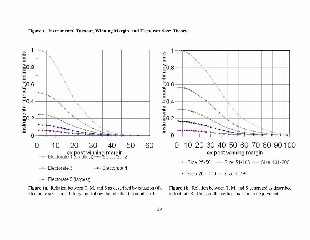
The equation can be interpreted directly, term by term, or its properties described using
simple heuristics. To do both, consider Figure 1a, which relates instrumental turnout to the winning
margin for five hypothetical electorates, constructed so each is twice as large as its predecessor (the
largest is sixteen times the size of the smallest). The bell curve shape of each line stems from the
quadratic in M, while the space between each line is controlled by the ln(S) term; the vertical scale
(which here is arbitrary) is determined by ß and the horizontal scale by F, set to a reasonable ten

None of the theoretical implications listed below are sensitive to the value of F. When5
F=10, precision about the winner’s percentage of the vote equals five percentage points, comparableto that estimated by Grant (1998) or to the margin of error in most political polls.
8
percentage points. The second term on the left-hand side is the general equilibrium “correction”5
that accounts for the effect of closeness on the number of voters used in calculating P. The term’s
effect depends on the magnitudes of T and T ; this is small when, as in the figure, the formerN I
dominates the latter.
The T, M, S relationship in Figure 1a is characterized as follows.
Implication 1: Turnout is negatively related to electorate size and the winning margin.
These well-supported predictions underlie the tests in equation (1). We call them “first-order”
predictions because they concern slope signs taken from first derivatives.
Implication 2: The negative relationship between turnout and the winning margin obtains
only over a limited range of M, above which it falls to zero. When the expected winning margin is
very large, incremental changes in this margin have little effect on P and hence little effect on
turnout. The (marginal) “tightening” of an election, in which the opposing sides become more
evenly matched, will affect turnout only if the election was expected to be fairly close to begin with.
Implication 3: The turnout/margin relationship is stronger in small electorates. The
tightening of an election is more likely to generate a tie when the number of voters is small. Thus,
in Figure 1a, the turnout/margin relation is strongest–steepest–in smaller electorates.
Implication 4: For any given margin, instrumental turnout is inversely proportional to
electorate size. In Figure 1a both electorate size and (roughly) the number of voters doubles when
moving from one electorate to its successor. With twice as many voters, one’s chances of casting
the deciding vote are twice as small: instrumental turnout should be cut in half. So, in the figure, the

9
height of adjacent curves halves as one moves downward to progressively larger electorates. The
inverse relation between P and N has been empirically confirmed by Mulligan and Hunter (2003).
These three “second-order” implications are one step more refined than Implication 1. Still,
they remain fundamental, not esoteric, model predictions: each is explained using simple heuristics
and justified with straightforward logic. If any of them are violated, the model is soundly rejected.
A two-stage estimation procedure assesses both these heuristic implications and the structural
equation they are based on. Each implication is directly tested with semiparametric methods that
essentially re-create Figure 1 with empirical estimates. The theory is rejected if any implication is
not satisfied. Then, using those estimates, one can easily estimate equation (6), which is linear in
suitably redefined parameters. The theory is rejected if there is significant misspecification. In
addition to the robustness already described, this two-stage approach has exceptional lucidity and
rigor. Semiparametric relations are more transparent than simple parameter estimates: if the model
fails, one learns which features are suitable and which are not. And specification tests incorporate
all model predictions, and so are more comprehensive than tests of coefficients alone. A structural
model could meet all assessment criteria used previously without satisfying Implications 1-4 or
passing a specification test.
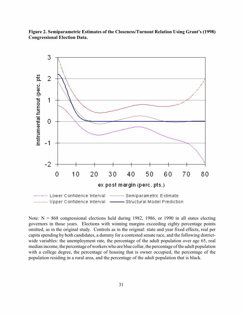
We illustrate with a brief, non-technical application of this methodology to the congressional
election data used in Grant (1998), to which we have access. (A brief description is found in the note
to Figure 2.) These electorates have similar sizes, so the S dimension is essentially eliminated;
semiparametric regression yields a single E(T )xM curve that should resemble those in Figure 1a,I
with a possible shift in horizontal scale. Deferring estimation details at present, Figure 2 shows the
semiparametric estimates and the associated estimated structural relation, based on equation (6),
10
which yields parameter estimates virtually identical to those in the original. The semiparametric
estimates closely match the theoretical predictions in Figure 1a, and the structural relation is clearly
not misspecified. With these data, one can ask no more of the model than this.
This example also illustrates the pertinence of the data issues raised earlier. Without much
(relative) S variation in these data, the study cannot test Implications 3 and 4, reducing its analytical
power. And with these electorates exceeding 100,000 voters, assessments of the reasonableness of
the closeness/turnout relation (a two percentage point increase in the closest elections), even at their
most rigorous, are inherently somewhat subjective. Both issues are eliminated in the data used here.
II. Union Certification Elections in the United States: 1994-2001.
Background. A union certification election is initiated when the National Labor Relations Board
(NLRB) is provided with the documented support of at least thirty percent of the employees in a
collective-bargaining unit, workers with a “community of interest” on the job. (See
http://www.nlrb.gov/nlrb/shared_files/brochures/engrep.asp. This method of initiating elections
raises selection issues, addressed in a footnote below, that turn out to be minor.) Bargaining units
are small: 98% have fewer than five hundred voters. The organization of small, employment-based
bargaining units along occupational lines makes these electorates relatively homogenous.
All workers in the bargaining unit are eligible to vote. The election, supervised by NLRB
agents, is conducted by secret ballot; challenges to voter eligibility are investigated by the NLRB.
Because firms and unions have strong incentives to scrutinize the conduct of the election and the
results are closely reviewed for irregularities, key variables are measured with little error, avoiding
11
an important source of bias (Cox, 1988). A majority is needed to certify the union, so a voter can
determine the electoral outcome by making a tie into a one-vote win for certification or vice versa.
As in political elections, both sides attempt to influence voters. Union tactics include house
calls and small group meetings; employer tactics include letters, meetings, and changes in
employment conditions (Bronfenbrenner, 1997). These efforts are focused on persuasion, not
mobilization, but can affect turnout by altering the perceived costs or benefits of unionizing. Their
magnitude will be determined by resource availability (Heneman and Sandver, 1989), the expected
effect of unionization on wages and profits, and the likelihood they will alter the electoral outcome.
Turnout will depend upon the costs of voting, the benefits of being the deciding voter, and
the probability of being decisive. Each differs greatly between political elections and union
certification elections. Voters in the former incur large transportation and waiting costs, both of
which are small in the latter, which are usually held at work and have few voters. On the other hand,
the benefit of deciding the outcome of a union certification election is substantial, as union
representation can greatly affect wages (by an average of 15-20%), employment security, working
conditions, and labor-management relations. (To any individual the net benefits of unionizing can
be positive or negative; all that matters is that the magnitude be large.) The benefits of choosing
one’s preferred political candidate are, at least, less tangible and less direct.
But the greatest distinction between the two types of elections concerns the probability of
casting the deciding vote. Here this is non-negligible, because union certification elections are small:
one vote would change the outcome of more than 2% of all elections in the sample and more than
15% of all elections with a winning margin under ten percentage points. In contrast, the comparable
probability was only 0.005% in the presidential contests studied by Nalebuff and Shachar (1999,

The data overlap the change in the classification scheme used by the Office and6
Management of Budget (OMB) to categorize establishments into industries. In 1997, the NAICSsystem replaced the SIC system. Although NAICS codes do not directly map to SIC codes, there isa rough correspondence among highly aggregated industries. The level of aggregation of the two-digit SIC codes is similar to that of the three-digit NAICS codes. Therefore, separate sets of dummyvariables at the two-digit SIC and three-digit NAICS level are used to identify the industry of thebargaining unit. See “Introducing NAICS” at http://www.dol.state.ga.us.
12
looking for ties at the state level) and the congressional elections studied by Grant (1998) and
Mulligan and Hunter (2003). The large expected instrumental benefits of voting in close union
certification elections should yield noticeable changes in turnout, making these elections suitable for
testing the theory. And they have other desirable features. Potential voters should be able to
estimate the closeness of the contest, because they work together and the election is held several
weeks after it is initiated. Also these are single issue elections, with no “third party candidates.”
Data. We study private sector union certification elections held in the U.S. between October, 1994
and September, 2001 using data maintained by the NLRB, available to the public upon request.
Screens were applied to remove multiple-unit elections, elections with missing data, and elections
held in U.S. territories. We also apply two screens with regard to electorate size. While the small
electorates in our data are an advantage, extremely small electorates may be problematic if social
pressures and coalition building dominate. Therefore we focus on elections with at least twenty-five
eligible voters, and also conduct some estimations on the subsample with at least one hundred
eligible voters. This leaves 9,854 observations in the full sample and 3,167 in the subsample. For
each election the data identifies the number of eligible voters, yea and nay votes for certification,
two-digit industry, union name, type of bargaining unit, election date, and geographic location. All6
these variables are used, either to calculate T, S, and M or for controls.

A control is also included for the fraction of potential voters whose eligibility is challenged;7
a successful challenge prevents those individuals from voting. The most important bias that mightbe introduced by insufficient controls concerns persuasion efforts, which should be related to P, asdiscussed above (see Nalebuff and Shachar, 1999, in a political context). To the extent they are notcaptured by the controls, the results will be biased in favor of the rational voting model, becausestrategic influence efforts will be ascribed to rational voting instead. This will ultimately strengthenthe paper’s conclusions, because the data provide only limited support for the model.
13
These controls, suggested by theory and by studies of union certification election outcomes
(Moranto and Fiorito, 1987), can be grouped into six categories: union characteristics, such as dues
or the extent of local control; firm and industry characteristics, such as profitability or injury rates;
worker characteristics, such as income or political philosophy; macroeconomic conditions, such as
unemployment; the legal environment, such as the presence of right to work laws; and union and
management organizing resources, as discussed previously. Some controls are measured directly:
the statewide, annual unemployment rate and the number of work stoppages in that state in that
month, both taken from the Bureau of Labor Statistics, and a dummy for a right-to-work law in that
state in that year. The others are proxied using sets of dummy variables identifying the union (151),
state (50), two-digit industry (159), type of bargaining unit (8), year (7), month (11), and day of the
week (6). Geographic dummies capture inter-state differences in the legal environment and political
philosophy; year dummies capture nationwide trends in the macroeconomy and in political attitudes;
union dummies capture differences in union characteristics and union resources; industry dummies
capture differences in industrial conditions; and the bargaining unit type variables proxy for
occupation, and thus for differences in worker socioeconomic status.7
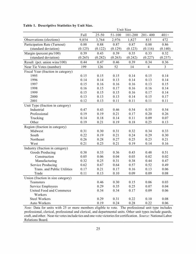
Descriptive Statistics. Table 1 contains descriptive statistics for the full sample and for five groups
of elections, based on electorate size, used in the formal analysis below. These are constructed as
14
in Figure 1a: the smallest group contains 25-50 eligible voters, and the range of eligible voters
doubles in each succeeding group. Table 1 shows that the elections in our sample are dispersed
geographically and in terms of industry, unit type, and union type.
While election outcomes are evenly divided–certification prevails 44% of the time–most
elections are not close. In Table 1 the average margin is thirty-nine percentage points, a 69.5%-
30.5% victory for the winning side. The coupling of large margins with divided outcomes might
reflect the relative homogeneity of the voters in union certification elections (Demsetz, 1993).
Homogeneity within the bargaining unit generates large margins, because voters with similar
characteristics tend to vote similarly; heterogeneity across units explains the divide in outcomes.
Voter turnout, averaging 88%, is far higher than in political elections, as expected. But this
high mean masks considerable variation: the standard deviation of turnout is 12.5 percentage points.
This variation does not conform to some conventions regarding turnout in political elections. In
Table 2, which tabulates election characteristics by fiscal year, unit type, region, industry, and union,
turnout is, if anything, higher in the South and lower among more educated (professional) workers,
and exhibits no downward trend (trends in outcomes are examined by Farber, 2001). The high
turnout mean suggests many workers are non-marginal in terms of the voting decision, and would
vote even if the outcome was certain. But the substantial standard deviation indicates there are also
many marginal voters who respond to changes in costs and benefits. The empirics will show how
these individuals respond to changes in P. While T >> T , T need not be zero.N I I
The high turnout and large margins observed here stand in sharp contrast to political elections
that are generally marked by voter apathy and smaller margins. Still, with small electorates and a
large sample, there are enough close elections that key parameters can be estimated with precision.

As in equation (10) in the Appendix, conditional P is calculated using the binomial8
distribution, with the number of voters used in this calculation calculated from M and S (in effectinstrumenting the number of voters with M and S), using the estimates in row 2 of Table 3.
15
In summary, these are the key differences between the two types of elections:
UNION CERTIFICATION ELECTIONS POLITICAL ELECTIONS
C small numbers of voters large numbers of votersC high benefit of voting, low cost high cost of voting, uncertain benefitC issues are primarily economic, not political issues are primarily politicalC homogenous electorates heterogenous electoratesC ties and near ties not infrequent ties and near ties quite rareC elections generated by petition elections held at regular intervals
Model Implications. The asymptotics in equation (2) assume large electorates, while we have
advocated the study of small electorates. This is not much of a problem. Equation (2) applies when
N >> 1/F², which should be satisfied even with only one thousand voters. When there are fewer, as
in our data, P is still approximately normal in M*, but “sampling error” inflates the variance of M
above F². (See the Appendix, Claim 2.) Thus, the functional form in equation (6) is still valid, only
F cannot be strictly interpreted as defined. Implications 1-4 depend only on this functional form and
will continue to hold.
To illustrate, the predicted T ,M,S relationship in our data is generated numerically,I
maintaining the same degree of uncertainty about candidate preferences (F = 0.10) as before, but
without using the large-electorate formula for P. This is graphed in Figure 1b, using the same8
format as Figure 1a. The two figures are not identical, and the vertical scale differs, as expected, but
the shapes of the curves and the relations between them, which generate Implications 1-4, remain.
To confirm the similarity in functional forms, we treat equation (6) as a regression in the
The model is estimated using OLS, which is traditional. Though some classical model9
assumptions are not strictly met, results are not sensitive to the estimation method used. Weightingthe observations by electorate size did not materially affect the results; neither did a tobit estimator.Repeat elections in the same bargaining unit generate correlated errors, but there are few of these.
16
parameters ß and F, and “fit” it to the points plotted in Figure 1b (scaling instrumental turnout so its
maximum is half of non-instrumental turnout, as in the actual data). The results are presented in the
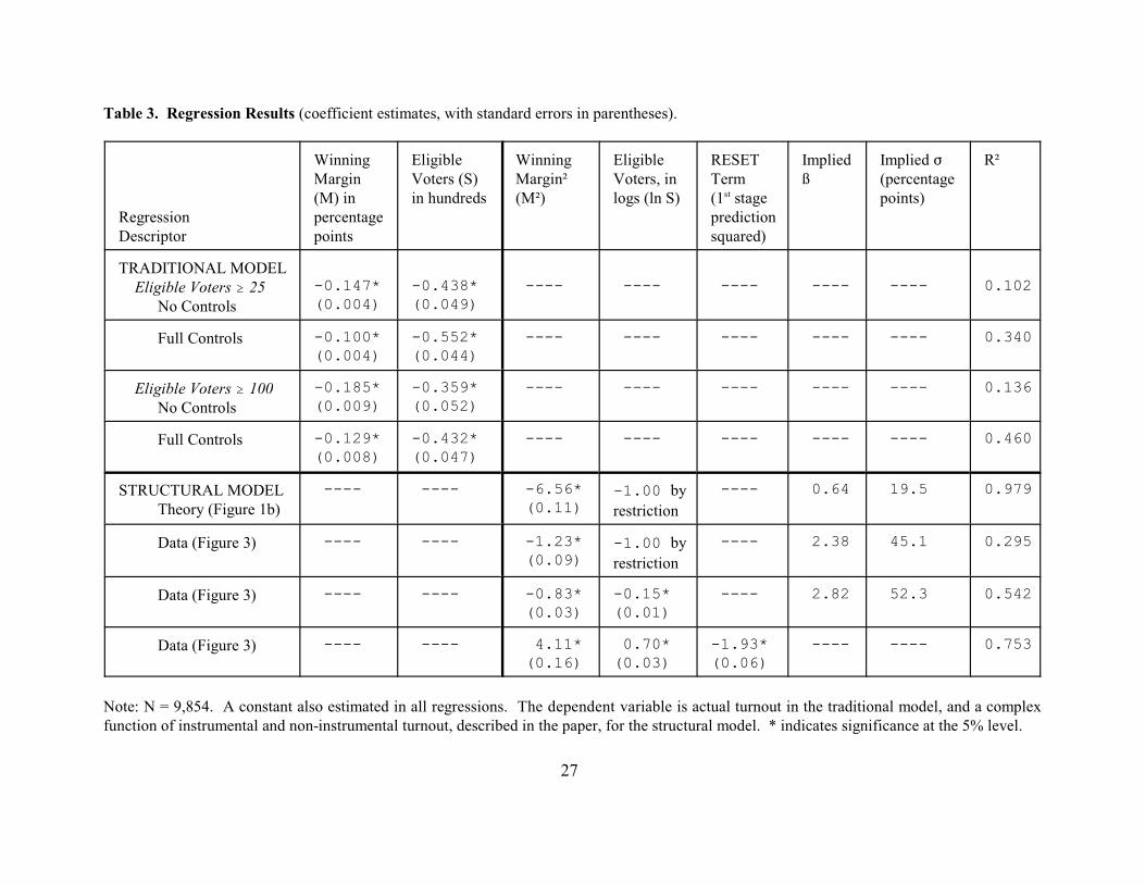
fifth row of Table 3. The true value of F is not obtained, reflecting the broader horizontal scale in
Figure 1b, but the fit is excellent. With just one free parameter (other than the constant, ß), R² is
0.98, and the correlation between actual and predicted T is virtually one. Equation (6) can be usedI
for specification tests in very small electorates, though the structural parameters cannot be recovered.
III. Estimation.
First Order Implications. Estimates of equation (1), which tests Implication 1, are presented in the
top panel of Table 3, for the full sample and for the subsample for which S $ 100, with and without
controls. The coefficients on M and S are always negative, as predicted, and highly significant;9
there is no material difference between the full sample and the subsample, as is the case with the rest
of the estimates we present. A ten percentage point increase in the winning margin, or two hundred
additional eligible voters, reduces turnout by about one percentage point. The predicted difference
in turnout between a hotly contested election involving one hundred voters and a lopsided election
involving one thousand voters is nearly twenty percentage points, one-fifth of the mean. Here, many
individuals vote only in close elections. As we have argued, this is reasonable given the importance
of the issue being decided and the significant possibility of a tie in a close election.

Sampling error in estimating these fixed effects inflates this standard deviation. To reduce10
this problem, the calculations omit unions and industries appearing in at most five observations.
For example, a linear regression of total turnout on M², to test Implication 2, an M*S11
interaction, to test Implication 3, and 1/S, to test Implication 4, will not work. The sign of M²T/MM²varies with M, so the hypothesized coefficient on the quadratic term is indeterminate, and the M*Sterm muddies the coefficient on 1/S. A double-log specification relating ln(T) to ln(N(M)), ln(S),and controls implies total turnout approaches zero as P vanishes, and is also unacceptable.
17
(7)
Further perspective on the turnout/closeness relationship can be obtained by comparing it to
the relation between turnout and other key factors: state, union, and industry. This is done by
calculating the standard deviation of the appropriate set of fixed effects. A one standard deviation10
change in M and S yields a 4.7 percentage point change in turnout. In contrast, the state fixed effects
have a standard deviation of 2.6 percentage points; the union fixed effects, 4.3 percentage points;
the industry fixed effects, 4.4 percentage points. The turnout/closeness relationship estimated here
is not just empirically significant; it is the strongest empirical regularity observed in these data.
Second Order Implications. To test the second order implications, we must uncover the T ,M,SI
relation in the data without imposing unnecessary functional form, as the functional form implied
by theory generates these implications to begin with. No natural reduced form specification will do
this. But semiparametric regression accurately reveals this relation without restriction.11
Here the controls enter parametrically, as before, but not the winning margin. Rather, turnout
gis an arbitrary function of M, f (M), for each of the five electorate size groups defined in Table 1:
i,gwhere i indexes elections and g electorate size groups, and the dummy D equals one if election i

The more general option is to estimate a surface representing instrumental turnout in12
T×M×S space. But estimation suffers from the curse of dimensionality and is infeasible, and theapproach adopted here is a more convenient way of depicting the data’s defiance of the theory in anyevent. However, electorate size was divided into more than five groups for the structural estimationconducted below. Groups were based on ln(S), which was partitioned into intervals of 0.1.
Figure 3 could be “distorted” by selection bias stemming from the requirement that 30%13
of employees in the bargaining unit support a petition in order to hold the election. Units disinclinedto unionize and large units will find it more difficult to meet this requirement. Of these units, thoseholding elections will have workers that are especially willing to participate in the certificationdecision. One way to determine whether selection bias drives the results is to distinguish union winsfrom union losses: selection problems should be smaller in units that support certification, becauseit should be easier to satisfy the petition requirement. When Figure 3 was replicated (separately) for
18
falls within group g and zero otherwise. This specification takes the form of a generalized additive
model (Hastie and Tibshirani, 1990), which allows quick estimation via spline smoothing techniques
(Yatchew, 2003). The theory is supported only if Implications 2-4 are all confirmed.12
1 5The results–estimates of f - f –are graphed in Figure 3, using the same format as Figure 1b,
with which they can be compared. Turnout is scaled to zero at the largest margin for the largest
electorate size group, so the vertical axis represents instrumental turnout, at least putatively.
Confidence intervals are discussed in the note but omitted from the graph, for clarity; the standard
errors, usually less than one percentage point, are small in absolute and relative terms.
All second-order implications of the model are contradicted. The negative relation between
winning margin and turnout obtains throughout the full range of winning margins, in contrast to
Implication 2; indeed, it is strongest for large margins, not small ones. It is also strongest in large
electorates, in contrast to Implication 3. Finally, the inverse relation between size and instrumental
turnout asserted in Implication 4 is not observed. Larger electorates do exhibit lower turnout, as in
Implication 1, but instrumental turnout is not halved when electorate size doubles. Turnout responds
to election closeness, but not in the way rational voting theory predicts.13
the subsamples of union wins and of union losses, however, the patterns described in the text werealways clearly visible. Therefore the results are not attributable to selection bias.
19
(8)
There is formal statistical support for these assertions. The “average slope” of each line in
Figure 3 is easily obtained; these can be compared using an F-test to formally assess Implication 3.
Here, the F statistic of 8.83 rejects the null of equal slopes at p < 0.01, but except for line D, these
slopes monotonically increase in magnitude, in contrast to theory. Statistical tests of the significance
of the nonlinearities in lines A-E are available in our statistical package (SAS). Each is statistically
significant at p << 0.01, but is also the opposite of that implied by theory. Formal tests of
Hypothesis 4 await the final step, structural estimation. These tests easily reject Implication 4.
Structural Estimation. One need not return to the original data to conduct structural estimation of
equation (6). With large samples, one can recast this equation as a regression employing the
semiparametric estimates as dependent variables, essentially “estimating” Figure 3. Least squares
can be used to do this, so computation is far simpler than in other general equilibrium voting models.
Using a general semiparametric form T = f(M,S) + 7X + , for notational simplicity,
recombine the terms estimated in equation (7) as follows:
MAXas long as P vanishes in unanimous elections in the largest electorates, of size S . The residual,
included in calculating T , is assumed to represent factors known to the agent but not the$ N
econometrician. As discussed in Section I, however, parameter estimates will be very similar if T$N
excludes the residual, and this is easily confirmed with our data.

20
(9)
When sampling error in the semiparametric estimates, 0, is small, ln(x+0) . ln(x) + 0/x.
0 0Substituting into equation (6), and defining T to be the empirical analog of E , yields:
This can be estimated using least squares. Heteroskedasticity exists, as the error term < contains
both sampling and specification error. But the latter may dominate given small sampling error, so
weighting using the standard errors on the semiparametric estimates may not be desirable.
2Estimating ( instead of restricting it to be -1 allows Implication 4 to be formally tested. As
previously discussed, the structural parameters ß and F can be directly recovered from this regression
in all but the smallest electorates, and specification tests can still be conducted even in these.
OLS estimates of equation (9) are presented at the bottom of Table 3. The coefficient
estimate on ln(S) is tiny, reflecting the weak relation already observed. The R² value, 0.57, reflects
the tremendous misspecification in equation (9); otherwise, R² would deviate from one only due to
sampling error in the semiparametric estimates, which is minute. Formal specification tests, against
parametric or nonparametric alternatives, can be conducted using standard methods; the covariance
matrix of the semiparametric estimates should be employed to give the tests proper power. These
are superfluous here, as Implications 2-4 were each decisively rejected, but for completeness Table
3 presents a simple RESET test, which strongly rejects the null of no specification error.
IV. Comparison with Other Voting Models.
21
The semiparametric regression reveals that the turnout/margin relationship in our data is
especially strong in large electorates and when the winning margin is large, and that instrumental
turnout is negatively related but not inversely proportional to electorate size. The failure of the
rational voter model to explain these heuristics motivates an inquiry into alternative explanations.
One final advantage of the methodology introduced here is that it facilitates such comparisons.
The brute force approach would be to formally test each alternative theory with our data.
This is prevented by their variety (which precludes an exhaustive comparison), their computational
complexity (many new theories require nonlinear, structural estimation), and their inexactness (some
theories do not specify the relation between turnout and election closeness). Our approach, instead,
is to compare the relationships predicted by alternative theories to the patterns revealed by the
semiparametric estimates, looking for a perfect match. Even when these relationships are not
precisely specified, one can often determine whether the patterns observed in our data are plausible.
We do this for three sets of self-interested voting theories that feasibly predict a positive
turnout/closeness relation: information theories such as Matsusaka (1995), group voting theories
such as Morton (1991), and theories of expressive voting (Brennan and Lomasky, 1993). (Ethical
or altruistic voting theories are omitted because they probably do not apply to union certification
elections.) None explains all the patterns in the data, for reasons that appear to be fundamental.
In Matsusaka’s (1995) information theory, the likelihood of voting is the product of P and
the potential voter’s confidence that his preferred choice is truly the best choice, in a world of
imperfect information about the “true” attractiveness of the options on the ballot. Left unspecified
is the relationship between winning margin and voter confidence. If these two quantities are
independent, the relationships between T, M, and S match those in the rational voter model. If voter
The idea being that a lopsided election means one candidate is pervasively viewed as being14
superior. The instrumental disincentive to vote at higher margins would be counterbalanced byincreased confidence in the “correctness” of one’s vote. Thus the turnout/margin relationship wouldbe even flatter at high margins, and possibly positive. These patterns do not match Figure 3.
22
confidence is greater at high margins, the patterns in Figure 3 still would not be replicated.14
Furthermore, this model predicts Implications 3 and 4, as S affects turnout only through P, and these
are also not reflected in the data.
Group voting models posit two opposing blocks of potential voters. Each decides how many
members to send to the polls in order to maximize the net expected benefits of the election to that
block (the expected benefits of electoral victory minus the costs of voting). Coate and Conlin (2004)
have successfully tested one such model, and Nalebuff and Shachar (1999) have successfully tested
a variant in which group turnout is generated by the mobilization efforts of elites. Turnout need not
be inversely proportional to electorate size in these models (though some predict turnout and
electorate size are unrelated, counter to our findings). But voting is still motivated instrumentally,
just at the level of the group instead of the individual, so Implication 2 should still hold. Turnout
should increase when the expected margin narrows, but the greatest increases should not occur at
large margins, as observed in our data. There is little benefit to increasing turnout from a block of
voters when an election is expected to be lopsided.
Finally, in expressive voting models, such as Brennan and Hamlin (1998), individuals vote
because they derive utility from expressing themselves, not because they expect to alter the outcome
of the election. The expected margin need not be of direct interest to expressive voters; any
turnout/margin relationship must result from a correlation between the winning margin and the
expressive benefit of voting. This is not specified in many variants of expressive voting theory, so
In the elections studied here, a larger margin may have utilitarian value by enhancing the15
union’s negotiating power. The authors experimented extensively with “augmented” expressivemodels of this type, in which the motivation to vote is to provide information about the preferencesof the electorate. These predict the observed relation between T and M, but Implication 3, whichis not observed, still holds.
23
the relationship between turnout and election closeness is similarly unspecified. (This is not needed
to test the theory; see Kan and Yang, 2001.) An exception is Schuessler (2000), which predicts
higher turnout in closer elections, as we observe. Furthermore, Schuessler’s model is sufficiently
general that the non-linearities between T and M observed in our data cannot be ruled out. But the
relation between turnout and electorate size does not appear to match the data. The expressive
motive in most models, including Schuessler’s, is independent of electorate size, so turnout should
not be negatively related to electorate size, as observed here.15
No theory yields a perfect match, though some outperform the rational voting model, and
might achieve success with further development (perhaps by letting electorate size influence
turnout). Thus, while we reject the rational voter model here, we do not have a ready replacement.
V. Conclusion.
In union certification elections, like political elections, closeness matters. Turnout is strongly
related to the two determinants of one’s chances of deciding the electoral outcome: the size of the
electorate and the winning margin. Turnout in the closest elections in our sample is much higher
than in their weakly contested counterparts, an economically reasonable finding given the high stakes
in these elections and the substantial probability an individual vote will be decisive in a close contest.
Rigorous tests require asking not just ask whether turnout responds to election closeness, but

24
how. In our data the turnout/margin relationship is especially strong for large electorates and large
winning margins, counter to rational voting theory, which predicts stronger relationships for small
electorates and small winning margins. And, while instrumental turnout is negatively related to
electorate size, the inverse relationship postulated is not observed. Something else must generate
these turnout patterns. A survey of alternative theories reveals none that can fully do so. Still, the
simple heuristics we have articulated can help guide future theoretical developments.
With straightforward, distinct theoretical predictions and abundant data, rational voting is
an auspicious area for empirical research. The existing literature has not fully capitalized on these
advantages: the interpretation of empirical results is often subject to question, because of the small
P problem or because the first-order implication being tested is not unique to rational voting theory,
while the complexity of other models can hinder their application elsewhere and obscure the role of
key modeling assumptions. The methodology presented here moves the literature closer to the ideal:
empirical tests that are transparent, rigorous, easily executed, and unambiguously interpreted.
25
Table 1. Descriptive Statistics by Unit Size.Unit Size
Full 25-50 51-100 101-200 201- 400 401+
Observations (elections) 9,854 3,764 2,976 1,827 815 472
Participation Rate (Turnout)(standard deviation)
0.88(0.125)
0.88(0.122)
0.87(0.129)
0.87(0.123)
0.88(0.116)
0.86(0.140)
Margin (percent pts/100)(standard deviation)
0.39(0.265)
0.43(0.282)
0.39(0.263)
0.35(0.242)
0.33(0.227)
0.32(0.237)
Result (pct. union wins/100) 0.44 0.47 0.46 0.39 0.34 0.36
Near Tie Votes (number) 199 126 52 14 4 3
Fiscal Year (fraction in category)1995199619971998199920002001
0.150.140.150.160.150.130.12
0.150.140.160.150.150.130.13
0.150.130.160.170.150.130.11
0.140.140.160.160.160.140.11
0.150.130.130.160.170.150.11
0.140.140.150.140.140.170.11
Unit Type (fraction in category)IndustrialProfessionalTrucking Other
0.470.190.140.19
0.430.190.180.21
0.460.210.140.19
0.540.170.110.18
0.550.200.090.25
0.540.260.070.13
Region (fraction in category) Midwest South Northeast West
0.310.220.260.21
0.300.190.280.23
0.310.210.270.21
0.320.240.250.19
0.340.290.230.14
0.330.300.210.16
Industry (fraction in category) Goods Producing
Construction Manufacturing
Service ProducingTrans. and Public UtilitiesTrade
0.380.050.320.620.170.11
0.330.060.250.670.210.13
0.360.040.310.640.170.10
0.430.030.380.570.160.09
0.480.020.440.520.130.09
0.510.020.470.490.060.08
Union (fraction in size category)TeamstersService EmployeesUnited Food and Commerce
WorkersSteel WorkersAuto Workers
0.460.290.34
0.290.19
0.300.350.34
0.310.24
0.150.250.17
0.220.28
0.060.070.09
0.100.22
0.030.040.06
0.080.06
Note: Data for units with 25 or more members eligible to vote. The professional unit type includesprofessional, clerical, professional and clerical, and departmental units. Other unit types include guards,craft, and other. Near-tie votes include ties and one-vote victories for certification. Source: National LaborRelations Board.

26
Table 2. Descriptive Statistics by Year, Unit Type, and Region.
ElectionsEligibleVoters
ParticipationRate Margin Result
Full Sample 9,854 117.3 (173.1) 0.88 (0.125) 0.39 (0.265) 0.44
Fiscal Year 1995199619971998199920002001
1,4581,3461,5161,5421,5001,3271,165
113.6 (157.4)113.3 (163.1)114.0 (165.4)117.0 (167.9)115.7 (154.0)132.0 (211.4)116.2 (193.0)
0.88 (0.118)0.88 (0.125)0.88 (0.127)0.87 (0.123)0.88 (0.117)0.87 (0.137)0.87 (0.125)
0.38 (0.261)0.41 (0.261)0.40 (0.272)0.38 (0.270)0.39 (0.272)0.37 (0.260)0.39 (0.258)
0.440.410.460.450.470.390.41
Unit TypeIndustrialProfessionalTruckingOther
4,6691,9171,4111,856
125.4 (170.1)131.0 (211.1) 89.4 (135.9)104.1 (157.0)
0.89 (0.120)0.87 (0.119)0.89 (0.104)0.84 (0.148)
0.37 (0.256)0.38 (0.261)0.39 (0.253)0.44 (0.293)
0.420.460.350.52
Region Midwest South Northeast West
3,0702,1692,5932,021
123.2 (190.7)132.9 (179.1)108.3 (155.5)103.0 (157.5)
0.89 (0.110)0.89 (0.129)0.86 (0.129)0.86 (0.130)
0.35 (0.249)0.39 (0.261)0.43 (0.284)0.39 (0.262)
0.390.420.480.48
Industry Goods Producing
Construction Manufacturing
Service ProducingTrans./Public Util.Trade
3,716 4443,1486,1371,7111,054
135.9 (199.6) 74.1 (90.2) 143.9 (207.0) 106.0 (153.8) 90.4 (118.3) 104.4 (154.6)
0.90 (0.118)0.78 (0.214)0.90 (0.083)0.86 (0.126)0.87 (0.118)0.89 (0.098)
0.36 (0.249)0.51 (0.306)0.34 (0.233)0.40 (0.273)0.37 (0.257)0.40 (0.252)
0.340.420.330.490.440.37
Union Teamsters Service Employees
United Food and Commerce Workers
Steel WorkersAuto Workers
1,996 575 494
440 340
93.9 (140.5)115.2 (136.6)129.6 (210.3)
142.2 (180.0)171.2 (197.9)
0.89 (0.100)0.83 (0.142)0.88 (0.097)
0.93 (0.068)0.92 (0.089)
0.38 (0.244) 0.43 (0.296) 0.37 (0.237)
0.30 (0.221) 0.28 (0.234)
0.34 0.67 0.47
0.38 0.49
Note: Standard deviations in parenthesis. Data are for units with 25 or more eligible voters. Theprofessional unit type includes professional, clerical, and departmental units. Other unit types includeguards, craft, and other. One extremely large election at Boeing in 2001 (17,000 eligible voters) is omittedbecause it substantially skews means and standard deviations in the categories in which it is included.Result and margin are defined as in Table 1. Source: National Labor Relations Board.
27
Table 3. Regression Results (coefficient estimates, with standard errors in parentheses).
Regression Descriptor
WinningMargin(M) inpercentagepoints
EligibleVoters (S)in hundreds
WinningMargin²(M²)
EligibleVoters, inlogs (ln S)
RESET Term (1 stagest
predictionsquared)
Impliedß
Implied F(percentagepoints)
R²
TRADITIONAL MODEL Eligible Voters $ 25
No Controls
-0.147*(0.004)
-0.438*(0.049)
---- ---- ---- ---- ---- 0.102
Full Controls -0.100*(0.004)
-0.552*(0.044)
---- ---- ---- ---- ---- 0.340
Eligible Voters $ 100No Controls
-0.185*(0.009)
-0.359*(0.052)
---- ---- ---- ---- ---- 0.136
Full Controls -0.129*(0.008)
-0.432*(0.047)
---- ---- ---- ---- ---- 0.460
STRUCTURAL MODELTheory (Figure 1b)
---- ---- -6.56* (0.11)
-1.00 by
restriction
---- 0.64 19.5 0.979
Data (Figure 3) ---- ---- -1.23* (0.09)
-1.00 by
restriction
---- 2.38 45.1 0.295
Data (Figure 3) ---- ---- -0.83* (0.03)
-0.15*(0.01)
---- 2.82 52.3 0.542
Data (Figure 3) ---- ---- 4.11* (0.16)
0.70*(0.03)
-1.93*(0.06)
---- ---- 0.753
Note: N = 9,854. A constant also estimated in all regressions. The dependent variable is actual turnout in the traditional model, and a complexfunction of instrumental and non-instrumental turnout, described in the paper, for the structural model. * indicates significance at the 5% level.

28
29
Figure 1. Instrumental Turnout, Winning Margin, and Electorate Size: Theory.
Figure 1a. Relation between T, M, and S as described by equation (6). Figure 1b. Relation between T, M, and S generated as describedElectorate sizes are arbitrary, but follow the rule that the number of in footnote 8. Units on the vertical axis are not equivalent

30
eligible voters in electorate g is twice that in electorate g-1. between the two graphs.
31
Figure 2. Semiparametric Estimates of the Closeness/Turnout Relation Using Grant’s (1998)Congressional Election Data.
Note: N = 868 congressional elections held during 1982, 1986, or 1990 in all states electinggovernors in those years. Elections with winning margins exceeding eighty percentage pointsomitted, as in the original study. Controls as in the original: state and year fixed effects, real percapita spending by both candidates, a dummy for a contested senate race, and the following district-wide variables: the unemployment rate, the percentage of the adult population over age 65, realmedian income, the percentage of workers who are blue collar, the percentage of the adult populationwith a college degree, the percentage of housing that is owner occupied, the percentage of thepopulation residing in a rural area, and the percentage of the adult population that is black.

32
Figure 3. Instrumental Turnout, Winning Margin, and Electorate Size: SemiparametricEstimates.
Note: Confidence intervals are not presented in the graph, for clarity, but are described here. Theyare generally narrow, and are smaller for smaller electorates and smaller margins, where there aremore observations. At M = 10 percentage points, the 95% confidence intervals in Lines A-E haveranges of ± 0.5, 0.6, 1.0, 1.0, and 1.3 percentage points, respectively. At M = 50 percentage points,the 95% confidence intervals in Lines A-E have ranges of ± 0.7, 0.8, 1.1, 1.4, and 1.8 percentagepoints, respectively. At M = 90 percentage points, the 95% confidence intervals in Lines A-E haveranges of ± 0.8, 1.2, 2.0, 2.8, and 3.4 percentage points, respectively. These intervals are narrowenough that the confidence intervals of adjacent lines sometimes do, and sometimes do not, overlap.

33
(10)
(11)
(12)
(13)
(14)
APPENDIX
Let P be one-half the probability of a tie vote (there is a 50% chance a tie would be broken inthe deciding voter’s favor), p be the actual probability any randomly chosen voter chooses the morepopular electoral option, and N be the actual number of voters (assumed to be even, as the extensionto odd N is trivial). If p is known with certainty, P is given by the binomial distribution:
Claim 1. Using Stirling’s formula, the combination term can be replaced with 2 (BN/2) ,N -½
generating:
Substituting the above into the identity T = ßP, taking logs, and rearranging as in the text yields:I
with the ex post winning margin M equal to 2p - 1 asymptotically. When T = 0, as in Coate,N
Conlin, and Moro (2004), this reduces to:
whose solution involves Lambert’s W function. Evaluating this solution for a wide range of S andM values generates the assertion in Section I that total turnout drops considerably as M grows awayfrom zero, so that the model cannot support realistic levels of turnout for both large and small M.A similar solution can be obtained for Hansen, Palfrey, and Rosenthal (1987), who restrict M=0instead. Recognize, however, that both of these studies adopt slightly different set-ups from thatused here, so these equations only approximate the outcomes of those other models.
Claim 2. If p is not known with certainty, one must determine the unconditional probabilityof casting the deciding vote, P, from the conditional probability in equation (10) and the distributionof p. The asymptotics have already been proved, as noted in the text, but the small electorate resultshave not yet been established. To derive these, begin with a first-order normal approximation toequation (10) above, adapted from Owen and Grofman (1984):
34
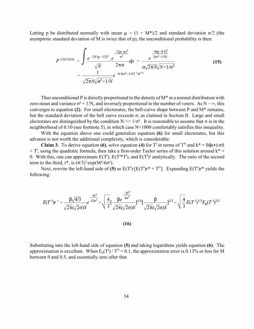
(15)
(16)
Letting p be distributed normally with mean : / (1 + M*)/2 and standard deviation F/2 (theasymptotic standard deviation of M is twice that of p), the unconditional probability is then:
Thus unconditional P is directly proportional to the density of M* in a normal distribution withzero mean and variance F² + 1/N, and inversely proportional to the number of voters. As N 6 4, thisconverges to equation (2). For small electorates, the bell-curve shape between P and M* remains,but the standard deviation of the bell curve exceeds F, as claimed in Section II. Large and smallelectorates are distinguished by the condition N >> 1/F². It is reasonable to assume that F is in theneighborhood of 0.10 (see footnote 5), in which case N=1000 comfortably satisfies this inequality.
With the equation above one could generalize equation (6) for small electorates, but thisadvance is not worth the additional complexity, which is considerable. Claim 3. To derive equation (6), solve equation (4) for T in terms of T and k* = ßN(C)/FSI N
< T , using the quadratic formula, then take a first-order Taylor series of this solution around k* =I
0. With this, one can approximate E(T ), E(T *T ), and E(T )² analytically. The ratio of the secondI I I I
term to the third, r*, is (4/3) exp(M²/6F²). ½
Next, rewrite the left-hand side of (5) as E(T )@[E(T )r* + T ]. Expanding E(T )r* yields theI I N I
following:
Substituting into the left-hand side of equation (5) and taking logarithms yields equation (6). The
0approximation is excellent. When E (T ) / T = 0.1, the approximation error is 0.13% or less for MI N
between 0 and 0.5, and essentially zero after that.

35
REFERENCES
Brennan, G., and Lomasky, L. Democracy and Decision. Cambridge: Cambridge University Press(1993).
Brennan, G., and Hamlin, A. “Expressive Voting and Electoral Equilibrium,” Public Choice 108,3,4: 295-312 (1998).
Bronfenbrenner, Kate. “The Role of Union Strategies in NLRB Certification Elections,” Industrialand Labor Relations Review 50, 2:195-212 (1997).
Chamberlain, Gary, and Michael Rothschild. "A Note on the Probability of Casting a DecisiveVote," Journal of Economic Theory 25:152-162 (1981).
Coate, Stephen, and Michael Conlin. “A Group Rule-Utilitarian Approach to Voter Turnout: Theoryand Evidence,” American Economic Review 94, 3:1476-1504 (2004).
Coate, Stephen, Michael Conlin, and Andrea Moro. “The Performance of the Pivotal-Voter Modelin Small-Scale Elections: Evidence from Texas Liquor Referenda.” NBER Working Paper10797 (2004).
Cox, Gary. "Closeness and Turnout: A Methodological Note," Journal of Politics 50:768-775(1988).
Demsetz, Rebecca. “Voting Behavior in Union Representation Elections: The Influence of SkillHomogeneity and Skill Group Size,” Industrial and Labor Relations Review 47:99-113 (1993).
Devinatz, Victor, and Daniel Rich. “Representation Type and Union Success in CertificationElections,” Journal of Labor Research 14, 1:85-92 (1993).
Downs, Anthony. An Economic Theory of Democracy. New York: Harper and Row (1957).
Farber, Henry. “Union Success in Representation Elections: Why Does Unit Size Matter?”Industrial and Labor Relations Review 54, 2:329-348 (2001).
Feddersen, Timothy. “Rational Choice Theory and the Paradox of Not Voting,” Journal ofEconomic Perspectives 18:99-112 (2004).
Fischer, A. “The Probability of Being Decisive,” Public Choice 101: 267-283 (1999).
Foster, Carroll. “The Performance of Rational Voter Models in Recent Presidential Elections,”American Political Science Review 78:678-690 (1984).
36
Good, I., and Lawrence Mayer. “Estimating the Efficacy of a Vote,” Behavioral Science 20, 1:25-33(1975).
Grant, Darren. “Searching for the Downsian Voter with a Simple Structural Model,” Economics andPolitics 10, 2:107-126 (1998).
Hansen, Stephen, Thomas Palfrey, and Howard Rosenthal. “The Downsian Model of ElectoralParticipation: Formal Theory and Empirical Analysis of the Constituency Size Effect,” PublicChoice 52, 1:15-33 (1987).
Hastie, T., and R. Tibshirani. Generalized Additive Models. New York: Chapman and Hall (1990).
Heneman, III, Herbert, and Marcus Sandver. “Union Characteristics and Organizing Success,”Journal of Labor Research 10,4:377-389 (1989).
Kan, Kamhon, and C.C. Yang. “On Expressive Voting: Evidence from the 1988 U.S. PresidentialElection,” Public Choice 108:295-312 (2001).
Margolis, Howard. “Probability of a Tied Election,” Public Choice 31:134-7 (1977).
Matsusaka, John, and Filip Palda. “The Downsian Voter Meets the Ecological Fallacy,” PublicChoice 77: 855-878 (1993).
Matsusaka, John. “Explaining Voter Turnout Patterns: An Information Theory,” Public Choice84:91-117 (1995).
Montgomery, B. Ruth. “The Influence of Attitudes and Normative Pressures on Voting Decisionsin a Union Certification Election,” Industrial and Labor Relations Review 42:263-279 (1989).
Moranto, Cheryl, and Jack Fiorito. “The Effects of Union Characteristics on the Outcome of UnionCertification Elections,” Industrial and Labor Relations Review 40:225-240 (1987).
Morton, Rebecca. “Groups in Rational Turnout Models,” American Journal of Political Science35:758-76 (1991).
Mueller, Dennis. Public Choice III. Cambridge: Cambridge University Press (2003).
Mulligan, Casey B and Charles G. Hunter. “The Empirical Frequency Of A Pivotal Vote,” PublicChoice 116:31-54 (2003).
Nalebuff, Barry and Ron Shachar. “Follow the Leader: Theory and Evidence on PoliticalParticipation,” American Economic Review 89, 3:525-547 (1999).

37
Noury, Abdul. “Abstention in Daylight: Strategic Calculus of Voting in the European Parliament,”Public Choice 212:179-211 (2004).
Owen, G., and B. Grofman. "To Vote or Not to Vote: The Paradox of Non-Voting," Public Choice42:311-325 (1984).
Palfrey, Thomas, and Howard Rosenthal. “Voter Participation and Strategic Uncertainty,” AmericanPolitcal Science Review 79:62-78 (1985).
Schuessler, Alexander. A Logic of Expressive Choice. Princeton: Princeton University Press (2000).
Seim, Katja. “An Empirical Model of Firm Entry with Endogenous Product-Type Choices,” RANDJournal of Economics, forthcoming.
Yatchew, Adonis. Semiparametric Regression for the Applied Econometrician. Cambridge:Cambridge University Press (2003).