1

Gaussian distributions on Riemannian symmetric spaces :statistical learning with structured covariance matrices

Salem Said, Hatem Hajri, Lionel Bombrun, Baba C. Vemuri

Abstract

The Riemannian geometry of covariance matrices has been essential to several successful applications, in computer vision, biomedical signaland image processing, and radar data processing. For these applications, an important ongoing challenge is to develop Riemannian-geometric toolswhich are adapted to structured covariance matrices. The present paper proposes to meet this challenge by introducing a new class of probabilitydistributions, Gaussian distributions of structured covariance matrices. These are Riemannian analogs of Gaussian distributions, which only samplefrom covariance matrices having a preassigned structure, such as complex, Toeplitz, or block-Toeplitz. The usefulness of these distributions stemsfrom three features : (1) they are completely tractable, analytically or numerically, when dealing with large covariance matrices, (2) they providea statistical foundation to the concept of structured Riemannian barycentre (i.e. Frechet or geometric mean), (3) they lead to efficient statisticallearning algorithms, which realise, among others, density estimation and classification of structured covariance matrices. The paper starts from theobservation that several spaces of structured covariance matrices, considered from a geometric point of view, are Riemannian symmetric spaces.Accordingly, it develops an original theory of Gaussian distributions on Riemannian symmetric spaces, of their statistical inference, and of theirrelationship to the concept of Riemannian barycentre. Then, it uses this original theory to give a detailed description of Gaussian distributionsof three kinds of structured covariance matrices, complex, Toeplitz, and block-Toeplitz. Finally, it describes algorithms for density estimation andclassification of structured covariance matrices, based on Gaussian distribution mixture models.

Index Terms

Structured covariance matrix, Riemannian barycentre, Gaussian distribution, Riemannian symmetric space, Gaussian mixture model

I. INTRODUCTION

Data with values in the space of covariance matrices have become unavoidable in many applications (here, the term covariance matrix istaken to mean positive definite matrix). For example, these data arise as “tensors” in mechanical engineering and medical imaging [1]–[3], or as“covariance descriptors” in signal or image processing and computer vision [4]–[6][7]–[10]. Most often, the first step in any attempt to analyse thesedata consists in computing some kind of central tendancy, or average : the Riemannian barycentre [1][3][11] (i.e. Frechet or geometric mean), theRiemannian median [5][6], the log-det or Stein centre [12][13], etc. Therefore, an important objective is to provide a rigorous statistical frameworkfor the use of these various kinds of averages. In the case of the Riemannian barycentre, this objective was recently realised, through the introductionof Gaussian distributions on the space of covariance matrices [14][15].

Gaussian distributions on the space of covariance matrices were designed to extend the useful properties of normal distributions, from theusual context of Euclidean space, to that of the Riemannian space of covariance matrices equipped with its affine-invariant metric described in [3].Accordingly, they were called “generalised normal distributions” in [14] and “Riemannian Gaussian distributions” in [15]. The most attractivefeature of these Gaussians distributions is that they verify the following property, which may also be taken as their definition,

defining property of Gaussian distributions : maximum likelihood is equivalent to Riemannian barycentre (1)

This is an extension of the defining property of normal distributions on Euclidean space, dating all the way back to the work of Gauss [16].Indeed, in a Euclidean space, the concept of Riemannian barycentre reduces to that of arithmetic average. By virtue of Property (1), efficientalgorithms were developed, which use Riemannian barycentres in carrying out prediction and regression [14][17], as well as classification anddensity estimation [18]–[20], for data in the space of covariance matrices.

The present paper addresses the problem of extending the definition of Gaussian distributions, from the space of covariance matrices to certainspaces of structured covariance matrices. The motivation for posing this problem is the following. The structure of a covariance matrix is ahighly valuable piece of information. Therefore, it is important to develop algorithms which deal specifically with data in the space of covariancematrices, when these are known to possess a certain structure. To this end, the paper introduces a new class of probability distributions, Gaussiandistributions of structured covariance matrices. These are Gaussian distributions which only sample from covariance matrices having a certainpreassigned structure. Using these new distributions, it becomes possible to develop new versions of the algorithms from [14][17][18]–[20], whichdeal specifically with structured covariance matrices.

In the following, Gaussian distributions of structured covariance matrices will be given a complete description for three structures : complex,Toeplitz, and block-Toeplitz. This is achieved using the following observation, which was made in [14][15]. The fact that it is possible to useProperty (1), in order to define Gaussian distributions on the space of covariance matrices, is a result of the fact that this space, when equippedwith its affine-invariant metric, is a Riemannian symmetric space of non-positive curvature. Starting from this observation, the following newcontributions are developed below, in Sections III, IV and V. These employ the mathematical background provided in Section II and Appendix A.

— In Section III : Gaussian distributions on Riemannian symmetric spaces of non-positive curvature are introduced. If M is a Riemanniansymmetric space of non-positive curvature, then a Gaussian distribution G(x, σ) is defined on M by its probability density function, with respectto the Riemannian volume element of M,

p.d.f. of a Gaussian distribution : p(x| x, σ) =1

Z(σ)× exp

[−d 2(x, x)

2σ 2

]x ∈M , σ > 0 (2)

where d :M×M→ R+ denotes Riemannian distance in M. In all generality, as long as M is a Riemannian symmetric space of non-positivecurvature, Proposition 1 provides the exact expression of the normalising factor Z(σ), and Proposition 2 provides an algorithm for samplingfrom the Gaussian distribution G(x, σ). Also, Propositions 3 and 4 characterise the maximum likelihood estimates of the parameters x and σ. Inparticular, Proposition 3 shows that definition (2) implies Property (1).

— In Section IV : as special cases of the definition of Section III, Gaussian distributions of structured covariance matrices are described forthree spaces of structured covariance matrices : complex, Toeplitz, and block-Toeplitz. Each one of these three spaces of structured covariancematrices becomes a Riemannian symmetric space of non-positive curvature, when equipped with a so-called Hessian metric [21]–[24],

Riemannian metric = Hessian of entropy (3)

where the entropy function, for a covariance matrix x, is H(x) = − log det(x), as in the case of a multivariate normal model [25]. For each oneof the three structures, the metric (3) is given explicitly, the normalising factor Z(σ) is computed analytically or numerically, and an algorithm forsampling from a Gaussian distribution with known parameters is provided, (these algorithms are described in Appendix B).

arX

iv:1

607.

0692

9v2

[m

ath.

ST]

12

May

201

7

2

— In Section V : efficient statistical learning algorithms are derived, for classification and density estimation of data in a Riemannian symmetricspace of non-positive curvature, M. These algorithms are based on the idea that any probability density on M, at least if sufficiently regular, canbe approximated to any desired precision by a finite mixture of Gaussian densities,

mixture of Gaussian densities : p(x) =

K∑κ=1

ωκ × p(x| xκ, σκ) (4)

where ω1, . . . , ωK > 0 satisfy ω1 + . . .+ωK = 1 and where each density p(x| xκ, σκ) is given by (2). A BIC criterion for selecting the mixtureorder K, and an EM (expectation-maximisation) algorithm for estimating mixture parameters (ωκ, xκ, σκ) are provided. Applied in the settingof Section IV, these lead to new versions of the algorithms in [15][18]–[20], which deal specifically with structured covariance matrices, and whichperform, with a significant reduction in computational complexity, the same tasks as the recent non-parametric methods of [26]–[28].

Table 1. below summarises some of the new contributions of Sections III and IV. The table is intended to help readers navigate directly todesired results.

The main geometric ingredient in the defining Property (1) of Gaussian distributions is the Riemannian barycentre. Recall that the Riemannianbarycentre of a set of points x1, . . . , xN in a Riemannian manifold M is any global minimiser xN of the variance function

variance function : EN (x) =1

N

N∑n=1

d 2(x, xn) (5)

where xN exists and is unique whenever M is a Riemannian space of non-positive curvature [29][30]. The Riemannian barycentre of covariancematrices arises when M = Pn , the space of n × n covariance matrices, equipped with its affine-invariant metric. Its existence and uniquenessfollow from the fact that Pn is a Riemannian symmetric space of non-positive curvature [14][15].

Due to its many applications, the Riemannian barycentre of covariance matrices is the subject of intense ongoing research [11][31][32]. Recently,attention has been directed to the problem of computing the Riemannian barycentre of structured covariance matrices [23][24][33]. This problemarises because if Y1, . . . , YN ∈ Pn are covariance matrices which have some additional structure, then their Riemannian barycentre YN need nothave this same structure [33]. In order to resolve this issue, two approaches have been proposed, as follows.

Note that a space of structured covariance matrices is the intersection of Pn with some real vector space V of n× n matrices. This is heredenoted V Pn = V ∩ Pn . The vector space V can be that of matrices which have complex, Toeplitz, or block-Toeplitz structure, etc. The firstapproach to computing the Riemannian barycentre YN of Y1, . . . , YN ∈ V Pn was proposed in [33]. It defines YN as a minimiser of the variancefunction (5) over V Pn , rather than over the whole of Pn . This is an extrinsic approach, since it considers V Pn as a subspace of Pn . By contrast,the second approach to computing YN is an intrinsic approach, proposed in [21]–[24]. It considers V Pn as a “stand-alone” Riemannian manifoldM = V Pn equipped with the Hessian metric (3). Then, YN is given by the general definition of the Riemannian barycentre, applied to thisRiemannian manifold M.

For the present paper, the intrinsic approach to the definition of the Riemannian barycentre of structured covariance matrices is preferred. Inthis approach, a space V Pn of structured covariance matrices is equipped with the Hessian metric (3). If V Pn is the space of complex, Toeplitz, orblock-Toeplitz covariance matrices, then it becomes a Riemannian symmetric space of non-positive curvature, when equipped with this metric [21]–[24]. In turn, this allows for the definition of Gaussian distributions, based on Section III. In general, note that V Pn is an open convex cone inthe real vector space V . If V Pn is moreover a homogeneous and self-dual cone, then it becomes a Riemannian symmetric space of non-positivecurvature, when equipped with a Hessian metric of the form (3), which is given in [21][34]. Thus, the definition of Gaussian distributions, basedon Section III, extends to any space V Pn of structured covariance matrices, whenever V Pn is a homogeneous and self-dual cone.

Throughout the following, the normalising factor Z(σ) appearing in (2) will play a major role. Proposition 1 establishes its two main properties :(i) although (2) contains two parameters x and σ, this normalising factor does not depend on x but only on σ, (ii) when expressed in terms of the“natural parameter” η = −1/2σ 2, this normalising factor is a strictly log-convex function. Proposition 3 shows these two properties are crucialingredients in the definition of Gaussian distributions. Precisely, if x1, . . . , xN are independent samples from a Gaussian distributions G(x, σ)given by (2), then the log-likelihood function for the parameters x and σ is given by

log-likelihood function of a Gaussian distribution : L(x, σ) = −N logZ(σ) −1

2σ2

N∑n=1

d 2(x, xn) (6)

Then, (i) guarantees that the defining Property (1) is verified. Indeed, since the first term in (6) does not depend on x, maximisation of L(x, σ)with respect to x is equivalent to minimisation of the sum of squared distances appearing in its second term. However, this is the same as thevariance function (5). On the other hand, (ii) guarantees that maximisation of L(x, σ) with respect to σ is equivalent to a one-dimensional convexoptimisation problem, (expressed as a Legendre transform in equation (28)). Note the exact expression of Z(σ) is given by formulae (19) and(22) in the Proof of Proposition 1. In [35], a Monte Carlo integration technique was designed which uses these formulae to generate the graph ofZ(σ). In Section IV, this technique is shown to effectively compute Z(σ) when the space M is a space of large structured covariance matrices.

In conclusion, it is expected that Gaussian distributions on Riemannian symmetric spaces of non-positive curvature will be valuable tools indesigning statistical learning algorithms which deal with structured covariance matrices. Such algorithms would combine efficiency with reducedcomputational complexity, since the main requirement for maximum likelihood estimation of Gaussian distributions is computation of Riemannianbarycentres, a task for which there exists an increasing number of high-performance routines. As discussed in Section V, this is the essentialadvantage of the definition of Gaussian distributions adopted in the present paper, over other recent definitions, also used in designing statisticallearning algorithms, such as those considered in [26]–[28].

Table 1. : Gaussian distributions on symmetric spaces and spaces of structured covariance matrices

Notation Riemannian metric Normalising factor Z(σ) Sampling algorithm

Section III :symmetric space M

(19) and (22)in Proposition 1

Algorithm 1.based on Proposition 2

Paragraph IV-A : n×ncomplex covariancematrices

Monte Carlointegration from (34h)

Algorithm 2.in Appendix BM = Hn Hessian metric (34b)

Paragraph IV-B : n×nToeplitz covariancematrices

Algorithm 3.in Appendix BM = Tn Hessian metric (37a) Analytic expression (37h)

Paragraph IV-C : n×nblock-Toeplitzcovariance matriceswith N ×N blocks

Monte Carlointegration from(40i) and (40j)

Algorithm 4.in Appendix BM = T Nn Hessian metric (40a)

3

II. MATHEMATICAL BACKGROUND ON RIEMANNIAN SYMMETRIC SPACES

This section gives five facts about Riemannian symmetric spaces, Facts 1–5 below, which will be essential for the following. These are herestated in their general form, but three concrete examples are presented in Section IV.

A Riemannian symmetric space is a Riemannian manifold M such that, for each point x ∈ M, there exists an isometry transformationIx :M→M whose effect is to reverse geodesic curves passing through x [36] (Chapter IV, Page 170). Any Riemannian symmetric space is aRiemannian homogeneous space, although the converse is not true. In particular, Riemannian symmetric spaces share in two important propertiesof Riemannian homogeneous spaces, given in Facts 1 and 2 below : invariance of distance, and invariance of integrals.

To say that M is a Riemannian homogeneous space means a Lie group G acts transitively and isometrically on M [36] (Chapter II, Page113). Each element g ∈ G defines a geometric transformation of M which maps each point x ∈ M to its image g · x. These transformationssatisfy the group action property,

( g1g2) · x = g1 · ( g2 · x) (7)

Then, transitivity of group action means that for any two points x and y of M, there exists g ∈ G such that g · x = y.When G acts onM transitively, one says thatM is a homogeneous space. Homogeneous spaces admit a general description, as the quotient of

G by a compact Lie subgroup H . Precisely, choose some point o ∈M as origin, and let H be the subgroup of all h ∈ G such that h · o = o [36](Chapter II, Page 113). Then, M is identified with the quotient G/H .

When G acts on M isometrically, the transformations x 7→ g · x preserve the Riemannian metric and Riemannian distance of M. Thisis expressed in Fact 1 below, which uses the following notation [37]. The Riemannian metric of M is denoted ds2. For x ∈ M, this definesa quadratic form : ds2

x(dx) = squared length of a displacement dx away from x. The Riemannian distance corresponding to the metric ds2 isdenoted d(x, y) for x, y ∈M. Fact 1 is not a theorem, but really part of the definition of a Riemannian homogeneous space [36].I Fact 1 (Invariant distance): For g ∈ G and x, y ∈M,

preservation of metric : z = g · x ⇒ ds2z(dz) = ds2

x(dx) (8a)

preservation of distance : d( g · x, g · y) = d(x, y) (8b)

Turning to Fact 2, recall that the Riemannian metric ds2 defines a Riemannian volume element dv [37]. Fact 1 states that the transformationsx 7→ g · x preserve the metric ds2. Therefore, these transformations must also preserve the volume element dv. This leads to the invariance ofintegrals with respect to dv, as follows [36] (Chapter X, Page 361).I Fact 2 (Invariant integrals): For any integrable function f :M→ R and g ∈ G,

preservation of volume :∫M

f(g · x) dv(x) =

∫M

f(x) dv(x) (9)

Facts 1 and 2 above hold for any Riemannian homogeneous space. The following fact 3 requires that M should have non-positive curvature. Thisguarantees the existence and uniqueness of Riemannian barycentres in M [29].

Let π be a probability distribution on M. The Riemannian barycentre of π is a point xπ defined as follows. Consider Eπ :M→ R+ ,

variance function : Eπ(x) =

∫M

d 2(x, z) dπ(z) (10)

The Riemannian barycentre xπ is then a global minimiser of Eπ . Fact 3 states that xπ exists and is unique [29] (Theorem 2.1., Page 659).I Fact 3 (Riemannian barycentre): Assume that M has non-positive curvature. For any probability distribution π on M, the Riemannian

barycentre xπ exists and is unique. Moreover, xπ is the unique stationary point of the variance function Eπ .Fact 2 above states that integrals with respect to the Riemannian volume element dv are invariant. However, it does not show how these integralscan be computed. This is done by the following Fact 4, which requires that M should be a Riemannian symmetric space of non-compact type.This means that the group G is a semisimple Lie group of non-compact type [36] (Chapter V). It should be noted that this property implies thatM has (strictly) negative curvature, so that Fact 3 holds true.

To state Fact 4, assume that G is a semisimple Lie group of non-compact type. Recall that H is a compact Lie subgroup of G. Let g and hdenote the Lie algebras of G and H respectively, and let g have the following Iwasawa decomposition [36] (see details in Chapter VI, Page 219),

Iwasawa decomposition : g = h + a + n (11)

where a is an Abelian subalgebra of of g, and n is a nilpotent subalgebra of g. Each x ∈ M can be written in the following form [36] (ChapterX),

polar coordinates : x = exp (Ad(h) a) · o a ∈ a , h ∈ H (12)

where exp : g → G is the Lie group exponential, and Ad is the adjoint representation. Here, it will be said that (a, h) are polar coordinates ofx, which is then written x = x(a, h) (this is an abuse of notation, since (a, h) are not unique, but it will provide useful intuition).

The following integral formula holds [36] (Chapter X, Page 382). It makes use of the concept of roots. These are linear mappings λ : a→ R,which characterise the Lie algebra g. For a minimal, introduction to this concept, see Appendix A.I Fact 4 (Integration in polar coordinates): For any integrable function f :M→ R,∫

Mf(x) dv(x) = C×

∫H

∫a

f(a, h)D(a) da dh (13)

where C is a constant which does not depend on the function f , dh is the normalised Haar measure on H and da is the Lebesgue measure on a.The function D : a→ R+ is given by

D(a) =∏λ>0

sinhmλ (|λ(a)|) (14)

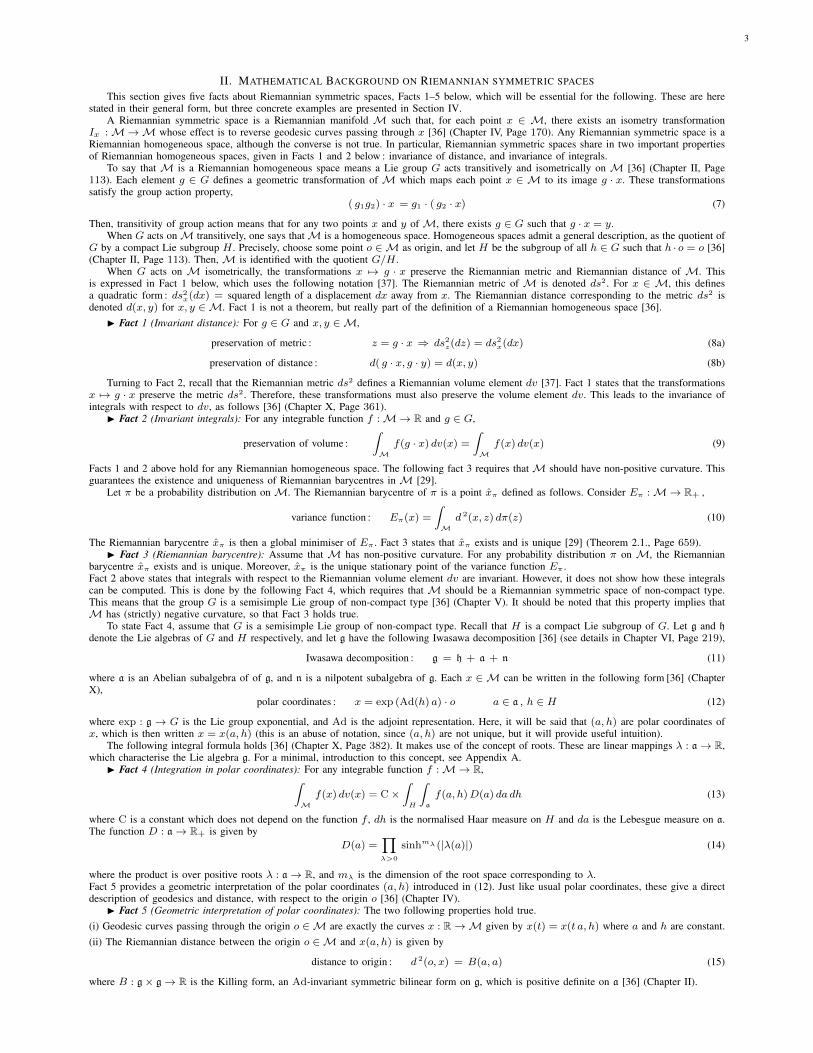
where the product is over positive roots λ : a→ R, and mλ is the dimension of the root space corresponding to λ.Fact 5 provides a geometric interpretation of the polar coordinates (a, h) introduced in (12). Just like usual polar coordinates, these give a directdescription of geodesics and distance, with respect to the origin o [36] (Chapter IV).I Fact 5 (Geometric interpretation of polar coordinates): The two following properties hold true.

(i) Geodesic curves passing through the origin o ∈M are exactly the curves x : R→M given by x(t) = x(t a, h) where a and h are constant.(ii) The Riemannian distance between the origin o ∈M and x(a, h) is given by

distance to origin : d 2(o, x) = B(a, a) (15)

where B : g× g→ R is the Killing form, an Ad-invariant symmetric bilinear form on g, which is positive definite on a [36] (Chapter II).

4

III. GAUSSIAN DISTRIBUTIONS ON RIEMANNIAN SYMMETRIC SPACES

This section introduces Gaussian distributions on Riemannian symmetric spaces, and studies maximum likelihood estimation of their parameters.These distributions establish a connection between the statistical concept of maximum likelihood estimation, and the geometric concept ofRiemannian barycentre.

Here, M is a Riemannian symmetric space of non-positive curvature. Recall d(x, y) denotes Riemanniain distance between x, y ∈ M, anddv denotes the Riemannian volume element of M. A Gaussian distribution is one that has the following probability density with respect to dv,

p(x| x, σ) =1

Z(σ)× exp

[−d 2(x, x)

2σ 2

](16)

where x ∈M and σ > 0. This distribution will be denoted G(x, σ).The main feature of the probability density (16) is that the normalising factor Z(σ) does not depend on the parameter x. This will be proved as

part of Proposition 1 below, and is the key ingredient in the relationship between Gaussian distributions and the concept of Riemannian barycentre.In [14][15], this relationship was developed in the special case where M = Pn , the symmetric space of real n × n covariance matrices. Thepresent paper considers the general case where M is any symmetric space of non-positive curvature. This allows for Gaussian distributions of theform (16) to be extended to spaces of structured covariance matrices, such as complex, Toeplitz, and block-Toeplitz covariance matrices, as donein Section IV below.

In the following, Paragraph III-A gives Proposition 1 which characterises the normalising factor Z(σ), and Proposition 2 which explains howto sample from a Gaussian distribution with given parameters. Paragraph III-B is concerned with maximum likelihood estimation of the parametersof a Gaussian distribution. In particular, it contains Proposition 3 which shows that the maximum likelihood estimate xN of the parameter xis precisely the Riemannian barycentre of available observations x1, . . . , xN . Finally, Proposition 4 can be used to obtain the consistency andasymptotic normality of xN .

A. Definition : the role of invarianceThis paragraph shows how the invariance properties of the Riemannian symmetric spaceM, described in Section II, can be used to characterise

Gaussian distributions onM. Precisely, for a Gaussian distribution G(x, σ), it is possible to obtain a) an exact expression of the normalising factorZ(σ) appearing in (16), and b) a generally applicable method for sampling from this distribution G(x, σ).

Proposition 1 is concerned with the normalising factor Z(σ). A fully general expression of Z(σ) is given by (19) and (22) in the proof ofthis proposition. To state Proposition 1, consider the following notation,

f(x| x, σ) = exp

[−d 2(x, x)

2σ 2

]Z(x, σ) =

∫M

f(x| x, σ) dv(x) (17)

In other words, f(x| x, σ) is the “profile” of the probability density p(x| x, σ).Proposition 1 (Normalising factor): The two following properties hold true.

(i) Z(x, σ) = Z(o , σ) for any x ∈M, where o is some point chosen as origin of M.(ii) Z(σ) = Z(o , σ) is a strictly log-convex function of the parameter η = −1/2σ 2.Proof : the proof of (i) follows from Facts 1 and 2. Since G acts transitively on M, any x ∈ M is of the form x = g · o for some g ∈ G.Applying (8b) from Fact 2 to (17), it then follows that f(x| x, σ) = f(g−1 · x| o , σ). Accordingly,

Z(x, σ) =

∫M

f(x| x, σ) dv(x) =

∫M

f(g−1 · x| o , σ) dv(x)

Now, by Fact 2, (and using g−1 instead of g in (9)),∫M

f(g−1 · x| o , σ) dv(x) =

∫M

f(x| o , σ) dv(x) = Z(o , σ)

so that (i) is indeed true. The proof of (ii) is based on Facts 4 and 5. Assume first thatM is a Riemannian symmetric space of non-compact type.By (13) and (15),

Z(σ) =

∫M

f(x| o , σ) dv(x) = C×∫H

∫a

exp

[−B(a, a)

2σ 2

]D(a) da dh (18)

But the function under the integral does not depend on h. Since dh is the normalised Haar measure on H ,

Z(σ) = C×∫a

exp

[−B(a, a)

2σ 2

]D(a) da (19)

In general, a Riemannian symmetric spaceM of non-positive curvature decomposes into a product Riemannian symmetric space [36] (Chapter V,Page 208),

M =M1 × . . .×Mr (20)

where each Mp is either a Euclidean space or a Riemannian symmetric space of non-compact type. Now, each x ∈ M is an r-tuple x =(x1, . . . , xr) where xp ∈Mp. Moreover, for x, y ∈M,

d 2(x, y) =r∑p=1

d 2p (xp , yp) (21)

where dp(xp , yp) is the Riemannian distance in Mp between xp and yp (where y = (y1, . . . , yr)). Replacing (21) in (17), it follows that,

Z(σ) = Z1(σ)× . . .× Zr(σ) (22)

where Zp(σ) is the normalising factor for the space Mp. Recall that a product of strictly log-convex functions is strictly log-convex. If Mp isa Euclidean space of dimension q, then Zp(σ) = (2πσ2)−q/2, which is a strictly log-convex function of η. If Mp is a Riemannian symmetricspace of non-compact type, Zp(σ) is given by (19). Let ρ = B(a, a) and µ(dρ) the image of D(a)da under the mapping a 7→ ρ. It follows that

Z(σ) = C ×∫ ∞

0

eη ρ µ(dρ) (23)

As a function of η , this is the moment-generating function of the positive measure µ(dρ), and therefore a strictly log-convex function [38], (Chapter7, Page 103). Thus, Z(σ) is a product (22) of strictly log-convex functions of η, and therefore itself strictly log-convex. This proves (ii).

5

The following Proposition 2 shows that polar coordinates (12) can be used to effectively sample from a Gaussian distribution G(x, σ). Thisproposition is concerned with the special case where M is a Riemannian symmetric space of non-compact type. However, the general case whereM is a Riemannian symmetric space of non-positive curvature can then be obtained using decomposition (20). This is explained in the remarkfollowing the proposition.

In the statement of Proposition 2, the following usual notation is used. If X is a random variable and P is a probability distibution, X ∼ Pmeans that X follows the probability distribution P .

Proposition 2 (Gaussian distribution via polar coordinates): Let M be a Riemannian symmetric space of non-compact type. Let M = G/Hwhere g has Iwasawa decomposition (11). Let h and a be independent random variables in H and a, respectively. Assume h is uniformly distributedon H , and a has probability density, with respect to the Lebesgue measure da on a,

p(a) ∝ exp

[−B(a, a)

2σ 2

]D(a) (24)

where ∝ indicates proportionality. The following hold true.(i) If x = x(a, h) as in (12), then x ∼ G(o, σ).(ii) If x ∼ G(o, σ) and x = g · o , then g · x ∼ G(x, σ).Proof : the proof of (ii) is a direct application of Fact 2, (compare to [15], proof of Proposition 5). Only the proof of (i) will be detailed. Thisfollows using Fact 4. Recall that a uniformly distributed random variable h in H has constant probability density, identically equal to 1, withrespect to the normalised Haar measure dh. Let h and a be as in the statement of the proposition. Since h and a are independent, (24) impliesthat for any function ϕ : H × a→ R, the expectation of ϕ(h, a) is equal to∫

H

∫a

ϕ(h, a) p(a) da dh ∝∫H

∫a

ϕ(h, a) exp

[−B(a, a)

2σ 2

]D(a) da dh

Then, if x = x(a, h) as in (12) and ϕ :M→ R, the expectation of ϕ(x) is proportional to,∫H

∫a

ϕ(x(h, a)) exp

[−B(a, a)

2σ 2

]D(a) da dh ∝

∫M

ϕ(x) p(x| o, σ) dv(x)

as follows from (13), (15) and (16). Since the function ϕ is arbitrary, this shows that the probability density of x with respect to dv is equal top(x| o, σ). In other words, x ∼ G(o, σ).

I Remark 1 : Proposition 2 only deals with the special case whereM is a Riemannian symmetric space of non-compact type. The general casewhereM is a Riemannian symmetric space of non-positive curvature is obtained as follows. LetM have decomposition (20) and x = (x1, . . . , xr)be a random variable in M with distribution G(x, σ). If x = (x1, . . . , xr), then it follows from (16) and (21) that

p(x| x, σ) = p(x1| x1, σ) × . . . × p(xr| xr, σ) (25)

Therefore, x1, . . . , xr are independent and each xp has distribution G(xp , σ). Conversely, (25) implies that if x1, . . . , xr are independent andeach xp has distribution G(xp , σ), then x has distribution G(x, σ).

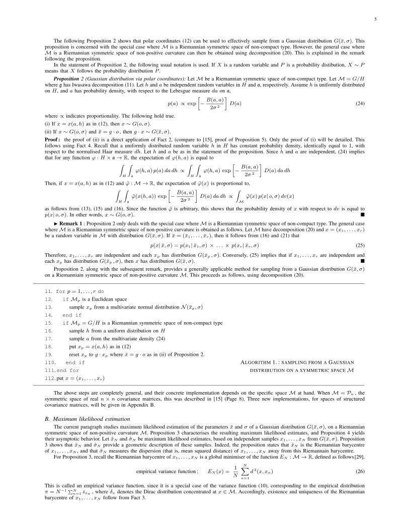
Proposition 2, along with the subsequent remark, provides a generally applicable method for sampling from a Gaussian distribution G(x, σ)on a Riemanniain symmetric space of non-positive curvature M. This proceeds as follows, using decomposition (20).

l1. for p = 1, . . . , r do

l2. ifMp is a Euclidean spacel3. sample xp from a multivariate normal distribution N (xp, σ)

l4. end if

l5. ifMp = G/H is a Riemannian symmetric space of non-compact typel6. sample h from a uniform distribution on Hl7. sample a from the multivariate density (24)l8. put xp = x(a, h) as in (12)l9. reset xp to g · xp where x = g · o as in (ii) of Proposition 2.l10. end if ALGORITHM 1. : SAMPLING FROM A GAUSSIAN

l11. end for DISTRIBUTION ON A SYMMETRIC SPACEMl12. put x = (x1, . . . , xr)

The above steps are completely general, and their concrete implementation depends on the specific space M at hand. When M = Pn , thesymmetric space of real n × n covariance matrices, this was described in [15] (Page 8). Three new implementations, for spaces of structuredcovariance matrices, will be given in Appendix B.

B. Maximum likelihood estimationThe current paragraph studies maximum likelihood estimation of the parameters x and σ of a Gaussian distribution G(x, σ), on a Riemannian

symmetric space of non-positive curvature M. Proposition 3 characterises the resulting maximum likelihood estimates, and Proposition 4 yieldstheir asymptotic behavior. Let xN and σN be maximum likelihood estimates, based on independent samples x1, . . . , xN from G(x, σ). Proposition3 shows that xN and σN provide a geometric description of these samples. Indeed, the proposition states that xN is the Riemannian barycentreof x1, . . . , xN , and that σN measures the dispersion (that is, mean squared distance) of x1, . . . , xN away from this Riemannain barycentre.

For Proposition 3, recall the Riemannian barycentre of x1, . . . , xN is a global minimiser of the function EN :M→ R, defined as follows[29],

empirical variance function : EN (x) =1

N

N∑n=1

d 2(x, xn) (26)

This is called an empirical variance function, since it is a special case of the variance function (10), corresponding to the empirical distributionπ = N−1 ∑N

n=1 δxn , where δx denotes the Dirac distribution concentrated at x ∈M. Accordingly, existence and uniqueness of the Riemannianbarycentre of x1, . . . , xN follow from Fact 3.

6

Proposition 3 (MLE and Riemannian barycentre): Let x1, . . . , xN be independent samples from G(x, σ). The maximum likelihood estimatesxN and σN , based on these samples, exist and are unique. Precisely,(i) xN is the Riemannian barycentre of x1, . . . , xN .(ii) There exists a strictly increasing bijective function Φ : R+ → R+, such that

σN = Φ(

1N

∑Nn=1d

2(xN , xn))

(27)

Proof : from (16), the log-likelihood function for the parameters x and σ is given by

L(x, σ) = −N logZ(σ) −1

2σ2

N∑n=1

d 2(x, xn)

By definition, xN and σN are found by maximising this function. The sum in the second term on the right hand side does not depend on σ.Therefore, xN can be found separately, by minimising this sum over the values of x (minimisation instead of maximisation is due to the minussign ahead of the sum). However, this is the same as minimising the empirical variance function (26). Now, the unique global minimiser of theempirical variance function is the Riemannian barycentre of x1, . . . , xN , whose existence and uniqueness follow from Fact 3 as noted before theproposition. This proves (i). Now, assume xN has been found. Then, to find σN , it is convenient to maximise L(xN , σ) over the values of theparameter η = −1/2σ 2 , which was already used in Proposition 1. Indeed, note that

1

NL(xN , σ) = η ρ− ψ(η)

where ρ = N−1 ∑Nn=1 d

2(xN , xn) and ψ(η) = logZ(σ). Thus, the maximum likelihood estimate ηN is given by

ηN = argmaxη η ρ− ψ(η) (28)

Recall that (ii) of Proposition 1 states that ψ is a strictly convex function, so its derivative ψ′ is strictly increasing. But, from (28), ηN is givenby ψ′(ηN ) = ρ. It follows that ηN exists and is unique, whenever ρ is in the range of ψ′. It is possible to show, using (23), that this range isequal to R+, which implies existence and uniqueness of ηN in general. Now, to complete the proof of (ii), it is enough to perform the change ofparameter from ηN back to σN .

Proposition 3 shows how the maximum likelihood estimates xN and σN can be computed, based on the samples x1, . . . , xN . Since xN is theRiemannian barycentre of these samples, xN can be computed using a variety of existing algorithms for computation of Riemannian barycentres.These include gradient descent [39][40], Newton method [41][42], recursive estimators [43][44], and stochastic methods [45][46]. Some of thesealgorithms are specifically adapted to Riemannian symmetric spaces of non-positive curvature (that is, to the context of the present paper) [42]–[44].Least computationally expensive are the recursive estimators [43][44]. On the other hand, the most computationally expensive, involving exactcalculation of the Hessian of squared Riemannian distance, is the Newton method of [42]. Computation of σN amounts to solving the equationψ′(ηN ) = ρ. This is a scalar non-linear equation, which can be solved using standard methods, such as the Newton-Raphson algorithm.

I Remark 2 : the entropy of a Gaussian distribution G(x, σ) is directly related to the function ψ introduced in the proof of Proposition 1.By definition, the entropy of G(x, σ) is [25],

h(x, σ) =

∫M

log p(x| x, σ)× p(x| x, σ) dv(x)

Using Fact 2 as in the proof of (i) in Proposition 1, it follows h(x, σ) = h(o, σ), so the entropy does not depend on x. Evaluataion of h(o, σ)gives, in the notation of (23),

h(o, σ) = C ×∫ ∞

0

(η ρ− ψ(η))× eη ρ−ψ(η) µ(dρ)

Following [38] (Chapter 9), let ψ∗ be the Legendre transform of ψ and ρ = ψ′(η). Then, the entropy h(o, σ) is equal to

entropy of a Gaussian distribution : ψ∗(ρ) = η ρ− ψ(η) (29)

Essentially, this is due to the fact that, when x is fixed, G(x, σ) takes on the form of an exponential distribution with natural parameter η andsufficient statistic ρ.

The following Proposition 4 clarifies the significance of the parameters x and σ of a Gaussian distribution G(x, σ). This Proposition is anasymptotic counterpart of Proposition 3. In particular, it can be used to obtain the consistency and asymptotic normality of xN . This is explainedin the remark after the proposition. For the statement of Proposition 4, recall the definition (10) of the variance function Eπ : M → R+ of aprobability distribution π on M. If π = G(x, σ), denote Eπ(x) = E(x| x, σ).

Proposition 4 (significance of the parameters): The parameters x and σ of a Gaussian distribution G(x, σ) are given by,

x is the Riemannian barycentre of G(x, σ) : x = argminx∈M E(x| x, σ) (30a)

σ = Φ(∫Md 2(x, z) p(z| x, σ) dv(z)

)(30b)

where Φ : R+ → R+ is the strictly increasing function introduced in Proposition 3.Proof : the proof can be carried out by direct generalisation of the one in [15] (proof of Proposition 9). An alternative, shorter proof of (30a),based on the definition of a Riemannian symmetric space, can be obtained by generalising [14] (proof of Theorem 2.3.).

I Remark 3 : Proposition 4 yields the consistency and asymptotic normality of the maximum likelihood estimate xN . Precisely,

consistency of xN : limN

xN = x (31a)

asymptotic normality of xN :√N Logx(xN )⇒ Nd(0 , C−1) (31b)

where Log denotes the Riemannian logarithm mapping [37], and Nd a normal distribtuion in d dimensions, (d being the dimension of M). Here,

C =∫M

(σ−2 Logx(z)

)⊗(σ−2 Logx(z)

)p(z| x, σ) dv(z) (32)

where ⊗ denotes exterior product of tangent vectors to M. Indeed, (31a) follows from Propositions 3 and 4. According to [47] (Theorem 2.3.,Page 8), the Riemannian barycentre xN of independent samples x1, . . . , xN from G(x, σ) converges to the Riemannien barycentre of G(x, σ).But this is exactly x. As for (31b), it can be proved by direct generalisation of the proof in [15] (Proposition 11).

7

IV. APPLICATION TO SPACES OF STRUCTURED COVARIANCE MATRICES

The previous Section III introduced the notion of a Gaussian distribution on a Riemannian symmetric space of non-positive curvature,M. In thepresent section, the development of Section III is applied to the special case whereM is a space of structured covariance matrices. Three variantsare considered : M = space of complex covariance matrices, M = space of Toeplitz covariance matrices, and M = space of block-Toeplitzcovariance matrices. In [14][15], Gaussian distributions were studied for M = space of real covariance matrices. Here, they are extended tospaces of covariance matrices with additional structure.

It seems that [21][22], in general, a space of structured covariance matrices becomes a Riemannian symmetric space of non-positive curvature,when it is equipped with a so-called Hessian metric. Roughly, a Hessian metric is a Riemannian metric arising from the entropy function,

Riemannian metric = Hessian of entropy (33)

where, ifM is a space of structured covariance matrices, the entropy of x ∈M is minus its log-determinant, H(x) = − log det(x) [25] (Chapter8, Page 254), as in the usual formula for the entropy of a multivariate normal distribution, with covariance x.

For each of the three variants mentioned above, the following development will be carried out. First, (33) is used to obtain a Riemannian metricds2 on M. It turns out that, as intended, this metric makes M into a Riemannian symmetric space of non-positive curvature. Second, Gaussiandistributions onM are characterised, as in Section III. Precisely, the graphs of the functions logZ : R+ → R and Φ : R+ → R+ are given basedon Propositions 1 and 3. Further, the reader is referred to Appendix B, for algorithms which provide samples from a Gaussian distribution on M.

A. Complex covariance matricesHere, M = Hn , the space of n× n complex covariance matrices. Precisely, each element Y ∈ Hn is an n× n Hermitian positive definite

matrix. This space Hn is equipped with a Hessian metric as follows.– Hessian metric : application of the general prescription (33) leads to a Riemannian metric on Hn which is identical to the well-known

affine-invariant metric, used in [48][3]. Indeed, the Hessian of the entropy function H(Y ) = − log det(Y ) has the following expression,

Hessian of entropy : D2H(Y )[v, w] = tr[Y −1v Y −1w

]Y ∈ Hn

for any complex matrices v and w, where tr denotes the trace. This expression can be found using the matrix differentiation formulae, as in [49](Appendix A, Page 196),

D log det(Y )[w] = tr[Y −1w

]DY −1[v] = −Y −1v Y −1 (34a)

Replacing in (33), gives the affine-invariant metric of Hn,

ds2Y (dY ) = D2H(Y )[dY, dY ] = tr

[Y −1dY Y −1dY

]Y ∈ Hn (34b)

The Riemannian distance corresponding to the metric (34b) has the following expression [48][3],

d 2(X,Y ) = tr[log(X−1/2Y X−1/2

)]2X,Y ∈ Hn (34c)

where all matrix functions, (matrix power and logarithm), are Hermitian matrix functions [50]. Moreover, the Riemannian volume element dv isgiven by, (this can be checked using [51], Lemma 2.1),

dv(Y ) = det(Y )−n∏i≤j

Re dYij∏i<j

Im dYij (34d)

where subscripts denote matrix elements, and Re and Im denote real and imaginary parts.– Symmetric space : equipped with the Riemannian metric (34b), Hn is a Riemannian symmetric space of non-positive curvature [36].

Accordingly, it is possible to apply Facts 1–5. To do so, note that G = GL(n,C), the Lie group of n × n invertible complex matrices, acts onHn transitively and isometrically by congruence transformations [48],

g · Y = g Y gH g ∈ G , Y ∈ Hn (34e)

where H denotes the conjugate transpose. Then, Facts 1 and 2 state that definitions (34b)–(34d) verify the general identities (8) and (9). Furthermore,Fact 3 states the existence and uniqueness of Riemannian barycentres in Hn.

The application of Facts 4 and 5 to Hn leads to the two following formulae, which are proved in Example 1 of Appendix A,∫Hn

f(Y ) dv(Y ) = C×∫U(n)

∫Rn

f(r, U)∏i<j

sinh2(|ri − rj |/2) dr dU (34f)

d 2(I, Y ) = ‖r‖2 =n∑j=1

r2j (I = n× n identity matrix) (34g)

For Hn, formulae (34f) and (34g) play the same role as formulae (13) and (15), for a general symmetric space M. Here Y = UerUH is thespectral decomposition of Y , with U ∈ U(n), the group of n × n unitary matrices, and er = diag(er1 , . . . , ern ) for r = (r1, . . . , rn) ∈ Rn.Moreover, dr denotes the Lebesgue measure on Rn and dU denotes the normalised Haar measure on U(n).

– Gaussian distributions : the functions logZ : R+ → R and Φ : R+ → R+, for Gaussian distributions on Hn, can be obtained usingformulae (34f) and (34g). These yield the following expression for Z(σ), similar to (18) in the proof of Proposition 1,

Z(σ) =

∫Hn

exp

[−d 2(I, Y )

2σ 2

]dv(Y ) = C×

∫U(n)

∫Rn

exp

[−‖r‖2

2σ 2

] ∏i<j

sinh2(|ri − rj |/2) dr dU

Since the function under the double integral does not depend on U , this integral simplifies to a formula similar to formula (19) in the proof ofProposition 1,

Z(σ) = C×∫Rn

exp

[−‖r‖2

2σ 2

] ∏i<j

sinh2(|ri − rj |/2) dr (34h)

For any moderate value of n, (in practice, up to n ≈ 40 has been considered), this formula can be numerically evaluated on a desktop computer,using a specifically designed Monte Carlo technique [35], leading to the graph of Z(σ). Then, obtaining the graphs of logZ : R+ → R andΦ : R+ → R+ is straightforward. In particular, it follows from (28) in the proof of Proposition 3 that the function Φ is obtained by solving, foreach ρ ∈ R+, the equation ρ = ψ′(η). Denoting η the unique solution of this equation, it follows that Φ(ρ) = σ where η = −1/2σ2.

8

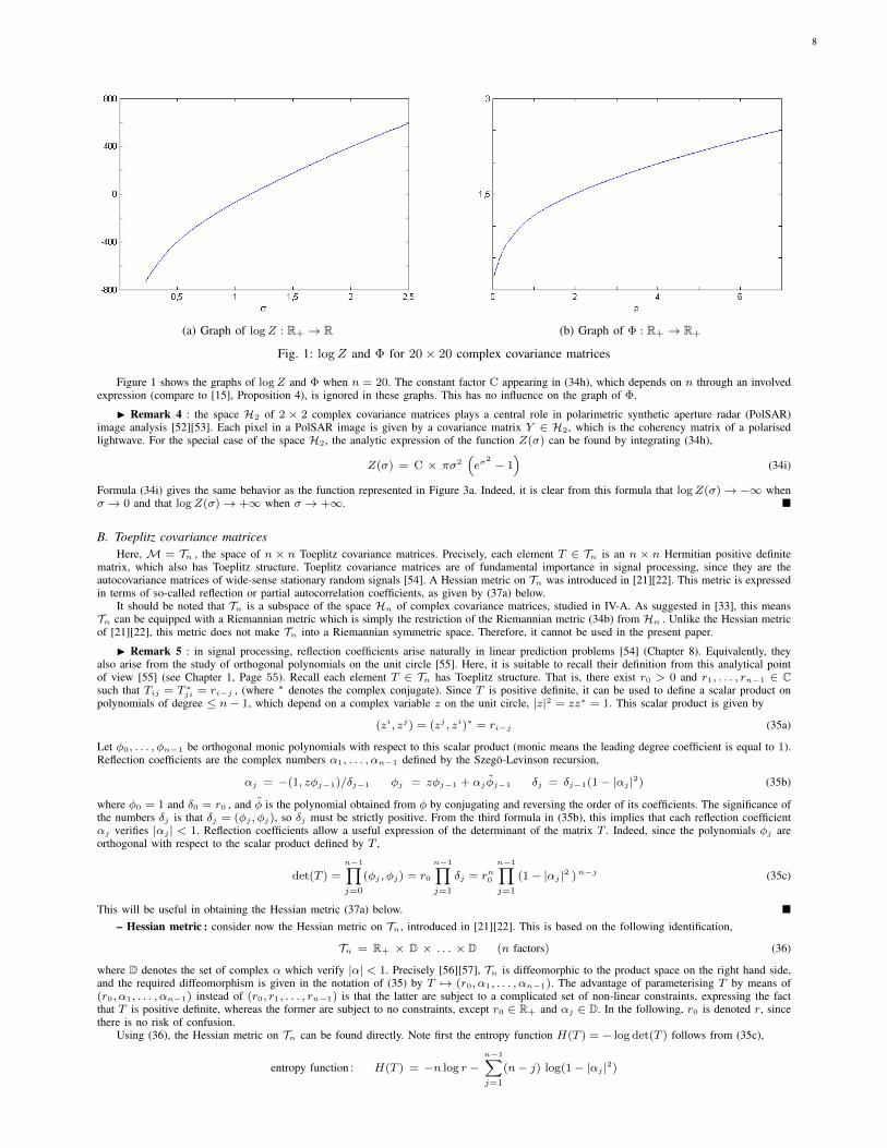
(a) Graph of logZ : R+ → R (b) Graph of Φ : R+ → R+

Fig. 1: logZ and Φ for 20 × 20 complex covariance matrices

Figure 1 shows the graphs of logZ and Φ when n = 20. The constant factor C appearing in (34h), which depends on n through an involvedexpression (compare to [15], Proposition 4), is ignored in these graphs. This has no influence on the graph of Φ.

I Remark 4 : the space H2 of 2 × 2 complex covariance matrices plays a central role in polarimetric synthetic aperture radar (PolSAR)image analysis [52][53]. Each pixel in a PolSAR image is given by a covariance matrix Y ∈ H2, which is the coherency matrix of a polarisedlightwave. For the special case of the space H2, the analytic expression of the function Z(σ) can be found by integrating (34h),

Z(σ) = C × πσ2(eσ

2 − 1)

(34i)

Formula (34i) gives the same behavior as the function represented in Figure 3a. Indeed, it is clear from this formula that logZ(σ)→ −∞ whenσ → 0 and that logZ(σ)→ +∞ when σ → +∞.

B. Toeplitz covariance matricesHere, M = Tn , the space of n × n Toeplitz covariance matrices. Precisely, each element T ∈ Tn is an n × n Hermitian positive definite

matrix, which also has Toeplitz structure. Toeplitz covariance matrices are of fundamental importance in signal processing, since they are theautocovariance matrices of wide-sense stationary random signals [54]. A Hessian metric on Tn was introduced in [21][22]. This metric is expressedin terms of so-called reflection or partial autocorrelation coefficients, as given by (37a) below.

It should be noted that Tn is a subspace of the space Hn of complex covariance matrices, studied in IV-A. As suggested in [33], this meansTn can be equipped with a Riemannian metric which is simply the restriction of the Riemannian metric (34b) from Hn . Unlike the Hessian metricof [21][22], this metric does not make Tn into a Riemannian symmetric space. Therefore, it cannot be used in the present paper.

I Remark 5 : in signal processing, reflection coefficients arise naturally in linear prediction problems [54] (Chapter 8). Equivalently, theyalso arise from the study of orthogonal polynomials on the unit circle [55]. Here, it is suitable to recall their definition from this analytical pointof view [55] (see Chapter 1, Page 55). Recall each element T ∈ Tn has Toeplitz structure. That is, there exist r0 > 0 and r1, . . . , rn−1 ∈ Csuch that Tij = T ∗ji = ri−j , (where ∗ denotes the complex conjugate). Since T is positive definite, it can be used to define a scalar product onpolynomials of degree ≤ n− 1, which depend on a complex variable z on the unit circle, |z|2 = zz∗ = 1. This scalar product is given by

(zi, zj) = (zj , zi)∗ = ri−j (35a)

Let φ0, . . . , φn−1 be orthogonal monic polynomials with respect to this scalar product (monic means the leading degree coefficient is equal to 1).Reflection coefficients are the complex numbers α1, . . . , αn−1 defined by the Szego-Levinson recursion,

αj = −(1, zφj−1)/δj−1 φj = zφj−1 + αj φj−1 δj = δj−1(1− |αj |2) (35b)

where φ0 = 1 and δ0 = r0 , and φ is the polynomial obtained from φ by conjugating and reversing the order of its coefficients. The significance ofthe numbers δj is that δj = (φj , φj), so δj must be strictly positive. From the third formula in (35b), this implies that each reflection coefficientαj verifies |αj | < 1. Reflection coefficients allow a useful expression of the determinant of the matrix T . Indeed, since the polynomials φj areorthogonal with respect to the scalar product defined by T ,

det(T ) =

n−1∏j=0

(φj , φj) = r0

n−1∏j=1

δj = rn0

n−1∏j=1

(1− |αj |2 )n−j (35c)

This will be useful in obtaining the Hessian metric (37a) below.

– Hessian metric : consider now the Hessian metric on Tn, introduced in [21][22]. This is based on the following identification,

Tn = R+ × D × . . . × D (n factors) (36)

where D denotes the set of complex α which verify |α| < 1. Precisely [56][57], Tn is diffeomorphic to the product space on the right hand side,and the required diffeomorphism is given in the notation of (35) by T 7→ (r0, α1, . . . , αn−1). The advantage of parameterising T by means of(r0, α1, . . . , αn−1) instead of (r0, r1, . . . , rn−1) is that the latter are subject to a complicated set of non-linear constraints, expressing the factthat T is positive definite, whereas the former are subject to no constraints, except r0 ∈ R+ and αj ∈ D. In the following, r0 is denoted r, sincethere is no risk of confusion.

Using (36), the Hessian metric on Tn can be found directly. Note first the entropy function H(T ) = − log det(T ) follows from (35c),

entropy function : H(T ) = −n log r −n−1∑j=1

(n− j) log(1− |αj |2)

9

Note the following elementary calculations,

∂2H

∂r2= n

1

r2

∂2H

∂αj ∂α∗j= (n− j)

[1− |αj |2

]−2

These immediately yield the Riemannian metric [21][22],

ds2T (dr, dα) = n

(dr

r

)2

+

n−1∑j=1

(n− j) ds2αj

(dαj) (37a)

where ds2α(dα) = |dα|2

/[1− |α|2

] 2α ∈ D

Here, ds2α is recognised as the Poincare metric on D [58] (Chapter III). Accordingly, the Riemannian distance and Riemannian volume element

on Tn have the following expressions,

d2(T (1), T (2)) = n∣∣log

(r(2)

)− log

(r(1)

) ∣∣2 +

n−1∑j=1

(n− j) d 2D (α

(1)j , α

(2)j ) (37b)

where dD(α, β) = atanh

∣∣∣∣ α− β1− α∗β

∣∣∣∣ α, β ∈ D

dv(T ) =√n∏n−1j=1 (n−j) ×

dr

r

n−1∏j=1

dv(αj) (37c)

where dv(α) =Re dα Im dα

[1− |α|2 ] 2 α ∈ D

Here, d 2D (α, β) and dv(α) denote the Riemannian distance and Riemannian volume element on D, corresponding to the Poincare metric ds2

α

appearing in (37a) [58].– Symmetric space : to see that the Riemannian metric (37a) makes Tn into a Riemannian symmetric space of non-positive curvature, it is

enough to notice that decomposition (36) is of the form (20), as in the proof of Proposition 1 in III-A. Indeed, in this decomposition, R+ appearsas a one-dimensional Euclidean space, by identification with R through the logarithm function, while each copy of D appears as a scaled versionof the Poincare disc, with the scale factor (n − j)1/2 , and therefore as a Riemannian symmetric space of non-compact type [58] (Chapter III),(the Poincare disc is the set D with the Poincare metric ds2

α , and is a space of constant negative curvature).To apply Facts 1–5 to Tn , consider the group G = R+ × SU(1, 1) × . . . × SU(1, 1), where SU(1, 1) is the group of 2 × 2 complex

matrices u such that

u =

(a bc d

): uT

(0 −11 0

)u =

(0 −11 0

), uH

(−1 00 1

)u =

(−1 00 1

)(37d)

with a, b, c, d ∈ C and T denotes the transpose. This group acts transitively and isometrically on Tn in the following way,

g · T = (s r, u1 · α1, . . . , un−1 · αn−1) , g = (s, u1, . . . , un−1) (37e)

where u · α =aα+ b

c α+ du ∈ SU(1, 1) , α ∈ D

Then, Facts 1 and 2 state that definitions (37a)–(37c) verify the general identities (8) and (9). Furthermore, Fact 3 states the existence and uniquenessof Riemannian barycentres in Tn.

The application of Facts 4 and 5 to Tn leads to the two following formulae, which are proved in Example 2 of Appendix A,∫Tn

f(T ) dv(T ) = C×∫ +∞

−∞

∫D. . .

∫Df(t, α1, . . . , αn−1) dv(α1) . . . dv(αn−1) dt (37f)∫

Df(α) dv(α) = C×

∫ 2π

0

∫ +∞

−∞f(ρ, θ) sinh(|ρ|)dρ dθ

d 2(I, T ) = n t2 +

n−1∑n=1

(n− j)ρ 2j (I = n× n identity matrix) (37g)

For Tn, formulae (37f) and (37g) play the same role as formulae (13) and (15), for a general symmetric space M. Here r = et and αj =tanh(ρj) e

iθj for j = 1, . . . , n− 1, where i =√−1.

– Gaussian distributions : using formulae (37f) and (37g), it is possible to find the exact analytic expression of the function logZ : R+ → Rfor Gaussian distributions on Tn. From this expression, which is given in (37i) below, the function Φ : R+ → R+ is found in the same waydiscussed in IV-A.

Unlike Gaussian distributions on Hn, for which the function logZ cannot be found analytically, but only using the Monte Carlo techniqueof [35], Gaussian distributions on Tn admit an exact analytic expression of logZ for any value of n. This means there is no computationallimitation on the size (given by n) of Toeplitz covariance matrices which can be modelled using Gaussian distributions.

Consider the calculation of Z(σ) using (37f) and (37g). Recall from (18) in the proof of Proposition 1,

Z(σ) =

∫Tn

exp

[−d 2(I, T )

2σ 2

]dv(T )

Upon replacing (37f) and (37g), this becomes,

Z(σ) = C×∫ +∞

−∞exp

[−n t2

2σ2

]dt ×

n−1∏j=1

∫ 2π

0

∫ +∞

−∞exp

[−

(n− j) ρ2j

2σ2

]sinh(|ρj |)dρj dθj

10

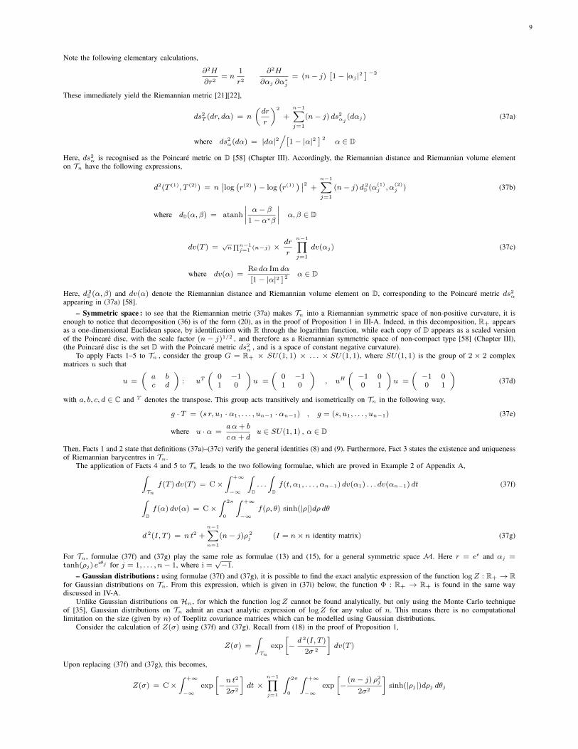
(a) Graph of logZ : R+ → R(b) Graph of Φ : R+ → R+

Fig. 2: logZ and Φ for 20 × 20 Toeplitz covariance matrices

by computing each integral in the product, it follows that

Z(σ) = C×√

2π/n σ ×n−1∏j=1

ZD

(σ/√

n− j)

(37h)

ZD(σ) = (2π)2/3 σ eσ2

2 × erf

(σ√

2

)where erf denotes the error function [59]. Finally, this yields the analytic expression of logZ,

logZ(σ) = C + log(σ/√

n)

+

n−1∑j=1

logZD(σ/√

n−j)

(37i)

Using (37h) and (37i), Figure 2 shows the graphs of logZ and Φ when n = 20. These graphs ignore the constant C appearing in (37i).

C. Block-Toeplitz covariance matricesHere,M = T Nn , the space of n×n block-Toeplitz covariance matrices which have N ×N Toeplitz blocks. Precisely, each element T ∈ T Nn

is an nN × nN Hermitian positive definite matrix, which has a block structure of the following form

T =

T0 T∗1 . . . T∗n−1

T1 T0 T∗1 . . . T∗n−2

T1 T0

......

...Tn−1 Tn−2 . . . T0

T0, . . . , Tn−1 ∈ TN

Block-Toeplitz covariance matrices which have Toeplitz blocks play a fundamental role in signal and image processing, where they arise in multi-channel and two-dimensional linear prediction and filtering problems [60][61]. A Hessian metric on T Nn was considered in [23], see (40a) below.This generalises the Hessian metric (37a) on the space Tn of Toeplitz covariance matrices, considered in the previous Paragraph IV-B. Precisely,in the same way as the metric (37a) was expressed in terms of scalar reflection coefficients α1, . . . , αn−1 which belong to the complex unit discD, the metric (40a) will be expressed in terms of matrix reflection coefficients Ω1, . . . ,Ωn−1 which belong to the matrix unit disc DN : the setof N × N symmetric complex matrices Ω which verify I − Ω∗Ω 0, where I denotes the N × N identity matrix and the Loewner order,(X Y means that X − Y is positive definite) [48].I Remark 6 : in signal and image processing, matrix reflection coefficients arise naturally in multi-channel and two-dimensional linear

prediction problems [60][61]. Here, they are introduced through the formalism of orthogonal matrix polynomials on the unit circle [62][63](compare to Remark 5, Paragraph IV-B). A matrix polynomial P on the unit circle is an expression P (z) = P0 + . . . + Pm zm, where z is acomplex variable on the unit circle, and P0, . . . , Pm are complex N × N matrices (here, m ≤ n − 1). Following [62] (Section 3, Page 43),consider for a fixed T ∈ T Nn the so-called left and right matrix scalar products of matrix polynomials. These are given by,

〈P zi , Qzj 〉L = P Ti−j QH 〈P zi , Qzj 〉R = PH Ti−j Q (38a)

for any complex N × N matrices P and Q , where Ti−j = T ∗j−i . Let ϕL0 , . . . , ϕLn−1 and ϕR0 , . . . , ϕ

Rn−1 be orthonormal matrix polynomials

with respect to these matrix scalar products. Matrix reflection coefficients Ω1, . . . ,Ωn−1 are given by the generalised Szego-Levinson recursion,

zϕLj−1 − ρjϕLj = ϕRj−1Ωj zϕRj−1 − ϕRj ρ∗j = ΩjϕLj−1 (38b)

where ρj = (I−Ω∗j Ωj )1/2, and where P , for a matrix polynomial P , denotes the polynomial obtained by taking the conjugate transposes of thecoefficients of P and reversing their order. It follows from [63] (Definition 2.3., Page 1615), that Ω1, . . . ,Ωn−1 ∈ DN . Moreover, Ω1, . . . ,Ωn−1

allow a useful expression of the determinant of the matrix T [23] (Page 10),

det(T ) = det(T0)nn−1∏j=1

det(I − Ω∗jΩj )n−j (38c)

This will be useful in obtaining the Hessian metric (40a) below.

11

– Hessian metric : consider now the Hessian metric on T Nn , introduced in [23]. This is based on the following identification,

T Nn = TN × DN × . . . × DN (n factors) (39)

where, as already stated, DN denotes the set of N × N symmetric complex matrices Ω which verify I − Ω∗Ω 0. Precisely [23], T Nn isdiffeomorphic to the product space on the right hand side, and the required diffeomorphism is given by T 7→ (T0,Ω1, . . . ,Ωn−1), in the notationof (38). In the following, T0 is denoted P , in order to avoid the unnecessary subscript.

Using (39), the Hessian metric on Tn can be found directly [23]. Note first the entropy function H(T ) = − log det(T ) follows from (38c),

entropy function : H(T ) = −n log det(P )−n−1∑j=1

(n− j) log det(I − Ω∗jΩj )

Then [23] (Page 10), applying the matrix differentiation formulae (34a) yields the required Hessian metric

ds2T (dP, dΩ) = nds2

P (dP ) +

n−1∑j=1

(n− j) ds2Ωj

(dΩj) (40a)

where ds2Ω(dΩ) = tr

[(I − ΩΩ∗)−1 dΩ (I − Ω∗Ω)−1 dΩ∗

]Ω ∈ DN

Here, ds2P is the Riemannian metric (37a) of the space TN , evaluated at P ∈ TN . On the other hand, ds2

Ω is recognised as the Siegel metric onDN [64]. Accordingly, the Riemannian distance and Riemannian volume element on Tn have the following expressions,

d 2(T (1), T (2)) = nd2TN

(P (1), P (2)) +

n−1∑j=1

(n− j) d 2DN

(Ω(1)j ,Ω

(2)j ) (40b)

where d 2DN

(Φ,Ψ) = tr[atanh2

(R1/2

)]R = (Ψ− Φ)(I − Φ∗Ψ)−1(Ψ∗ − Φ∗)(I − ΦΨ∗)−1 Φ,Ψ ∈ DN

Here, d2TN

(P (1), P (2)) is the Riemannian distance (37b) between P (1), P (2) ∈ TN .

dv(T ) =√n∏n−1j=1 (n−j) × dvTN (P )

n−1∏j=1

dv(Ωj) (40c)

where dv(Ω) =

∏i≤j Re dΩij Im dΩij

det (I − ΩΩ∗)N+1Ω ∈ DN

Here, dvTN (P ) is the Riemannian volume element (37c) computed at P ∈ TN . In expressions (40b) and (40c), d 2DN

(Φ,Ψ) and dv(Ω) denotethe Riemannian distance and Riemannian volume element on DN , corresponding to the Siegel metric ds2

Ω appearing in (40a). These may be foundin [23] (Page 10) and [65] (Chapter IV, Page 84), respectively.

– Symmetric space : to see that the Riemannian metric (40a) makes T Nn into a Riemannian symmetric space of non-positive curvature, itis enough to notice that decomposition (39) identifies T Nn with a product of Riemannian symmetric spaces of non-positive curvature. The firstfactor in this decomposition is the space TN of Toeplitz covariance matrices. This was seen to be a Riemannian symmetric space of non-positivecurvature in the previous Paragraph IV-B. Each of the remaining factors is a copy of DN , equipped with a scaled version of the Siegel metric ds2

Ω,as in (40a). With this metric, DN is a Riemannian symmetric space of non-compact type, known as the Siegel disc [36] (Exercice D.1., Page 527).

To apply Facts 1–5 to T Nn , consider the group G = GTN × Sp(n,R) × . . . ×Sp(n,R), where GTN = R+ × SU(1, 1) × . . . × SU(1, 1),as in (37d)–(37e) of Paragraph IV-B, and where Sp(n,R) is the group of 2N × 2N complex matrices U such that [64] (Page 10),

U =

(A BC D

): UT

(0 −II 0

)U =

(0 −II 0

), UH

(−I 00 I

)U =

(−I 00 I

)(40d)

with A,B,C,D complex N ×N matrices. This group G acts transitively and isometrically on T Nn in the following way,

g · T = (S · P ,U1 · Ω1, . . . , Un−1 · Ωn−1) , g = (S,U1, . . . , Un−1) (40e)

where U · Ω = (AΩ +B)(C Ω +D)−1 U ∈ Sp(n,R) , Ω ∈ DN

where S · P is given by (37e) for S ∈ GTN and P ∈ TN . Then, Facts 1 and 2 state that definitions (40a)–(40c) verify the general identities (8)and (9). Furthermore, Fact 3 states the existence and uniqueness of Riemannian barycentres in T Nn .

The application of Facts 4 and 5 to T Nn leads to the two following formulae, which are proved in Example 3 of Appendix A,∫TNn

f(T ) dv(T ) = C×∫TN

∫DN

. . .

∫DN

f(P,Ω1, . . . ,Ωn−1) dv(Ω1) . . . dv(Ωn−1) dvTN (P ) (40f)

∫DN

f(Ω) dv(Ω) = C×∫SU(N)

∫RN

f(r,Θ)∏i<j

sinh(|ri − rj |)∏i≤j

sinh(|ri + rj |) dr dΘ

d 2(I, T ) = nd2TN

(I, P ) +

n−1∑j=1

(n− j) d 2DN

(I,Ωj) (I = nN × nN identity matrix) (40g)

d 2DN

(I,Ω) = ‖r‖2 =

n∑j=1

r2j

For T Nn , formulae (40f) and (40g) play the same role as formulae (13) and (15), for a general symmetric spaceM. Here, dvT (P ) and d2TN

(I, P )are given by (37f) and (37g). Moreover, Ω ∈ DN is written in the form,

Ω = Θ tanh(r) ΘT tanh(r) = diag (tanh(r1), . . . , tanh(rn)) (40h)

where Θ ∈ SU(N), the group of unitary N × N matrices which have unit determinant, and r ∈ RN (this is called the Takagi factorisationin [66]). In (40f), dr denotes the Lebesgue measure on RN and dΘ denotes the normalised Haar measure on SU(N).

12

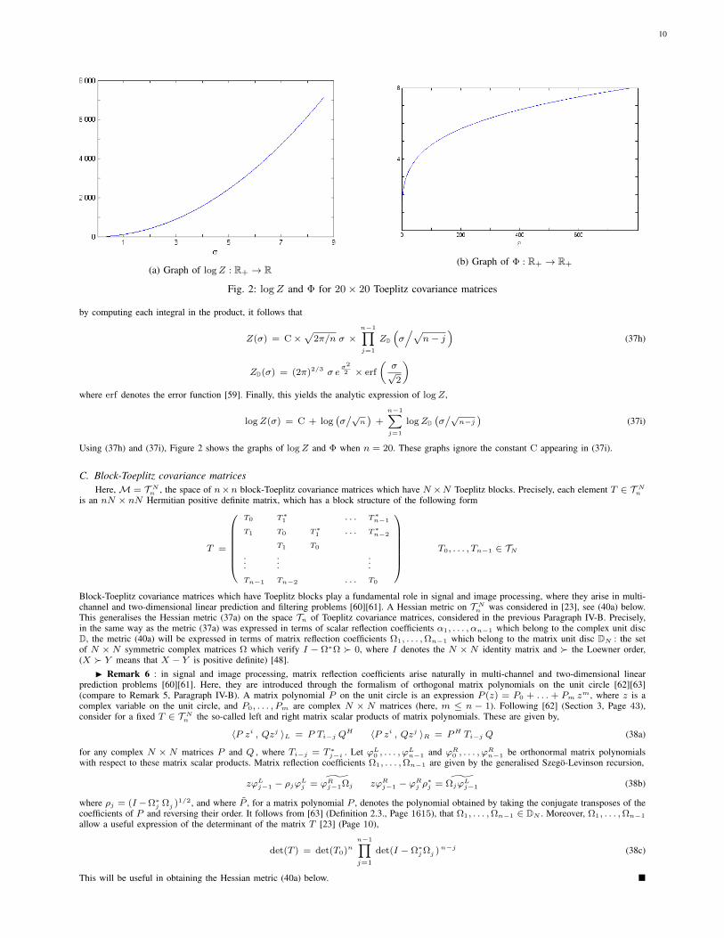
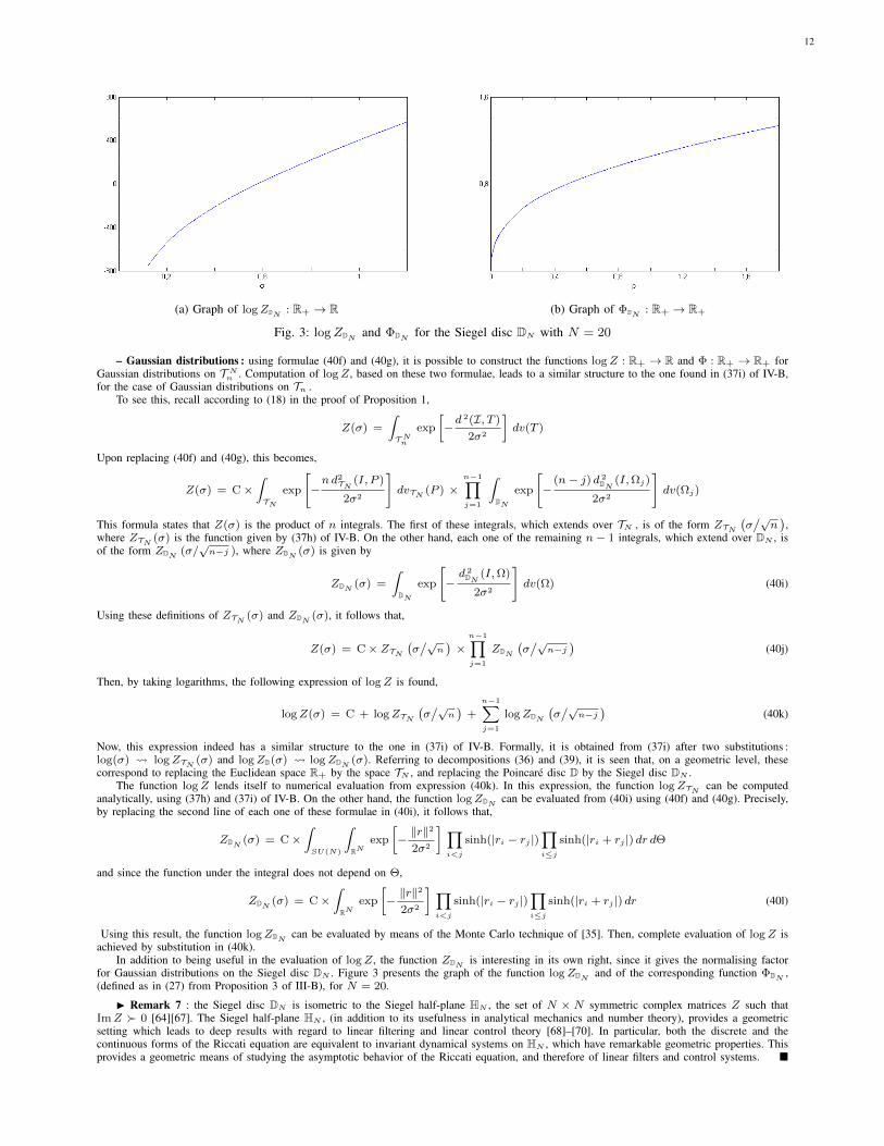
(a) Graph of logZDN : R+ → R (b) Graph of ΦDN : R+ → R+

Fig. 3: logZDN and ΦDN for the Siegel disc DN with N = 20

– Gaussian distributions : using formulae (40f) and (40g), it is possible to construct the functions logZ : R+ → R and Φ : R+ → R+ forGaussian distributions on T Nn . Computation of logZ, based on these two formulae, leads to a similar structure to the one found in (37i) of IV-B,for the case of Gaussian distributions on Tn .

To see this, recall according to (18) in the proof of Proposition 1,

Z(σ) =

∫TNn

exp

[−d 2(I, T )

2σ2

]dv(T )

Upon replacing (40f) and (40g), this becomes,

Z(σ) = C×∫TN

exp

[−nd2TN

(I, P )

2σ2

]dvTN (P ) ×

n−1∏j=1

∫DN

exp

[−

(n− j) d 2DN

(I,Ωj)

2σ2

]dv(Ωj)

This formula states that Z(σ) is the product of n integrals. The first of these integrals, which extends over TN , is of the form ZTN(σ/√

n),

where ZTN (σ) is the function given by (37h) of IV-B. On the other hand, each one of the remaining n− 1 integrals, which extend over DN , isof the form ZDN (σ/

√n−j ), where ZDN (σ) is given by

ZDN (σ) =

∫DN

exp

[−d 2DN

(I,Ω)

2σ2

]dv(Ω) (40i)

Using these definitions of ZTN (σ) and ZDN (σ), it follows that,

Z(σ) = C× ZTN(σ/√

n)×n−1∏j=1

ZDN

(σ/√

n−j)

(40j)

Then, by taking logarithms, the following expression of logZ is found,

logZ(σ) = C + logZTN(σ/√

n)

+

n−1∑j=1

logZDN

(σ/√

n−j)

(40k)

Now, this expression indeed has a similar structure to the one in (37i) of IV-B. Formally, it is obtained from (37i) after two substitutions :log(σ) logZTN (σ) and logZD(σ) logZDN (σ). Referring to decompositions (36) and (39), it is seen that, on a geometric level, thesecorrespond to replacing the Euclidean space R+ by the space TN , and replacing the Poincare disc D by the Siegel disc DN .

The function logZ lends itself to numerical evaluation from expression (40k). In this expression, the function logZTN can be computedanalytically, using (37h) and (37i) of IV-B. On the other hand, the function logZDN can be evaluated from (40i) using (40f) and (40g). Precisely,by replacing the second line of each one of these formulae in (40i), it follows that,

ZDN (σ) = C×∫SU(N)

∫RN

exp

[−‖r‖2

2σ2

] ∏i<j

sinh(|ri − rj |)∏i≤j

sinh(|ri + rj |) dr dΘ

and since the function under the integral does not depend on Θ,

ZDN (σ) = C×∫RN

exp

[−‖r‖2

2σ2

] ∏i<j

sinh(|ri − rj |)∏i≤j

sinh(|ri + rj |) dr (40l)

Using this result, the function logZDN can be evaluated by means of the Monte Carlo technique of [35]. Then, complete evaluation of logZ isachieved by substitution in (40k).

In addition to being useful in the evaluation of logZ, the function ZDN is interesting in its own right, since it gives the normalising factorfor Gaussian distributions on the Siegel disc DN . Figure 3 presents the graph of the function logZDN and of the corresponding function ΦDN ,(defined as in (27) from Proposition 3 of III-B), for N = 20.

I Remark 7 : the Siegel disc DN is isometric to the Siegel half-plane HN , the set of N × N symmetric complex matrices Z such thatImZ 0 [64][67]. The Siegel half-plane HN , (in addition to its usefulness in analytical mechanics and number theory), provides a geometricsetting which leads to deep results with regard to linear filtering and linear control theory [68]–[70]. In particular, both the discrete and thecontinuous forms of the Riccati equation are equivalent to invariant dynamical systems on HN , which have remarkable geometric properties. Thisprovides a geometric means of studying the asymptotic behavior of the Riccati equation, and therefore of linear filters and control systems.

13

V. DENSITY ESTIMATION WITH FINITE MIXTURES OF GAUSSIAN DENSITIES

The present section introduces finite mixtures of Gaussian densities, as a tool for dealing with the problem of density estimation in a Riemanniansymmetric space of non-positive curvature, M. A finite mixture of Gaussian densities on M is a probability density of the form

p(x) =

K∑κ=1

ωκ × p(x| xκ, σκ) (41)

where the weights ω1, . . . , ωK > 0 are such that ω1 + . . .+ ωK = 1, and where each density p(x| xκ, σκ) is a Gaussian density given by (16)of Section III. Definition (41) is directly based on the standard definition of a finite mixture of probability densities [71][72].

The problem of density estimation in M is the following [73][74]. Assume a population of data points x1, . . . , xN ∈ M is under study.Assume further this population was generated from some unknown probability density q(x). The problem is to approximate this unknown densityusing the data x1, . . . , xN .

Concretely, this problem arises in the following manner [18]–[20] [26]–[28]. As in Section IV, the spaceM is a space of structured covariancematrices. For example, M = Hn, M = Tn, or M = T Nn , (recall these notations from Table 1. in the introduction). A database of signalsor images is under study, and each object in this database is represented by a covariance descriptor. This descriptor is taken to be a structuredcovariance matrix x ∈ M. The database of signals or images is thus mapped into a population x1, . . . , xN ∈ M. In a real-world setting, it ishopeless to attempt any simplifying hypothesis with regard to the probability density q(x) of this population. Rather, one attempts to approximateq(x) within a sufficiently rich class of candidate densities p(x).

The use of mixtures of Gaussian densities as a tool for solving this problem is founded on the idea that the probability density q(x), at leastif sufficiently regular, can be approximated to any precision by a density p(x) of the form (41). Accordingly, consider the mathematical problemof finding a density p(x) of the form (41) which best approximates the unknown density q(x), in the sens of Kullback-Leibler divergence. Recallthis is given by [25],

p = argminp D(q ‖ p) D(q ‖ p) =

∫M

q(x) log

[q(x)

p(x)

]dv(x) (42)

where dv is the Riemannian volume element of M. Here, the minimum is over all densities p(x) of the form (41). Following the general idea of“empirical risk minimisation” [73] (Page 32), the above integral with respect to the unknown density q(x) is replaced by an empirical average.The minimisation problem (42) is then replaced by

pN = argminp1

N

N∑n=1

log

[q(xn)

p(xn)

]= argminp −

1

N

N∑n=1

log p(xn) (43)

This new minimisation problem is equivalent to the problem of maximum likelihood estimation of the parameters (ωκ, xκ, σκ) ; κ = 1, . . . ,Kof the finite mixture of Gaussian densities p(x), under the assumption that the data x1, . . . , xN are independently generated from p(x).

In [15], an original EM (expectation maximisation) algorithm was proposed for solving this problem of maximum likelihood estimation. Thisalgorithm was derived in the special case whereM = Pn , the space of n×n covariance matrices. It was successfully applied to real data, mainlyfrom remote sensing, with the aim of carrying out density estimation as well as classification [18]–[20]. This algorithm generalises directly fromM = Pn to any M which is a Riemannian symmetric space of non-positive curvature, and its derivation remains formally the same as in [15](Paragraph IV.A., Page 13).

In the present general setting, it can be described as follows. The algorithm assumes that K, the number of mixture components in (41),has already been selected. It iteratively updates an approximation θ = (ωκ, xκ, σκ) of the maximum likelihood estimates of the parameters(ωκ, xκ, σκ). The required update rules (45a)–(45c), as given below, are repeated as long as this leads to a sensible increase in the joint likelihoodfunction of (ωκ, xκ, σκ). These update rules involve the two quantities πκ(xn, θ) and Nκ(θ), defined as follows,

πκ(xn, θ) ∝ ωκ × p(xn| xκ, σκ) Nκ(θ) =

N∑n=1

πκ(xn, θ) (44)

where the constant of proportionality, corresponding to “∝” in the first expression, is chosen so ∑κ πκ(xn, θ) = 1. Each iteration of the EM

algorithm consists in an application of the updatte rules,

EM update rules for mixture estimation :

ωnewκ = Nκ(θ)

/N (45a)

xnewκ = argminx∈M Eκ(x) Eκ(x) = N−1κ (θ)

N∑n=1

πκ(xn, θ) d2(x, xn) (45b)

σnewκ = Φ(Eκ(xnewκ )) Φ given by (27) of Proposition 3 (45c)

Realisation of update rules (45a) and (45c) is straightforward. On the other hand, realisation of update rule (45b) requires minimisation ofthe function Eκ(x) over x ∈ M. It is clear this function is a variance function of the form (10), corresponding to the probability distributionπ∝

∑Nn=1 πκ(xn,θ)×δxn where δx denotes the Dirac distribution concentrated at x ∈ M. Therefore, existence and uniqueness of xnewκ follow

from Fact 3, and computation of xnewκ can be carried out using existing routines for the computation of Riemannian barycentres [40][42][44][45].The EM algorithm just described requires prior selection of the number K of mixture components. When this EM algorithm was applied

in [18]–[20], (for the special case M = Pn) , K was selected by maximising a BIC criterion. In general, this criterion is given following [75],

BIC criterion : K∗ = argmaxK BIC(K) BIC(K) = `(K) −1

2DF × ln(N) (46)

Here, `(K) is the maximum value of the joint likelihood function of (ωκ, xκ, σκ) for given K, and DF is the number of parameters to beestimated, or number of degrees of freedome. This is DF = K × [ 2 + dim(M) ] − 1. For the three spaces of structured covariance matricesconsidered in Section IV, the dimension of M is given by,

dim(Hn) = n2 dim(Tn) = 2n− 1 dim(T Nn ) = 2N − 1 + (n− 1)× (N2 +N) (47)

14

The EM algorithm given by update rules (45a)–(45c), and the BIC criterion (46), together provide a complete programme for solving the problemof density estimation in M, using finite mixtures of Gaussian densities. The output of this programme is an approximation of the finite mixtureof Gaussian densities pN defined by (43). Then, with a slight abuse of notation, it is possible to write,

pN (x) =K∑κ=1

ωκ × p(x| xκ, σκ) (48)

In [15][18]–[20], an additional problem of classification was addressed, whose aim is to use (48) as an explicative model of the data x1, . . . , xN ,revealing the fact that these data arise from K disjoint classes, where the κth class is generated from a single Gaussian distribution G(xκ, σκ).In [15] (Paragraph IV.B., Page 15), this problem was solved in the special case M = Pn . In general, the proposed solution remains valid aslong as M is a Riemannian symmetric space of non-positive curvature. It is based on a Bayes optimal classification rule. This is a functionκ∗ :M→ 1, . . . ,K , obtained by minimising the a posteriori probability of classification error [74] (Section 2.4., Page 21),

κ∗(x) = argminκ=1,...,K [ 1− P (κ|x) ] (49)

where P (κ|x) is found from Bayes rule, P (κ|x) ∝ p(x|κ)×P (κ), after replacing p(x|κ) = p(x| xκ, σκ) and P (κ) = ωκ , where p(x| xκ, σκ)is given by (16). Carrying out the minimisation (49) readily gives the expression,

κ∗(x) = argminκ=1,...,K

[− log ωκ + log Z(σκ) +

d 2(x, xκ)

2σ2κ

](50)

This is a generalisation of the so-called minimum-distance-to-mean classification rule, which corresponds to all ωκ and all σκ being constant, (inthe sense that they do not depend on κ). In [4], the minimum-distance-to-mean classification rule was shown to give very good performance inthe area brain-computer interface decoding. Ongoing work, started in [35], examines the application of (50) in this same area.

Comparison to kernel density estimationIn recent literature [26]–[28], a fully non-parametric method for density estimation inM was developed. This is based on the method of kernel

density estimation on Riemannian manifolds, first outlined in [76]. This non-parametric method is alternative to the method of the present section,based on finite mixtures of Gaussian distributions. Currently, no practical comparison of these two methods is available, as they have not yet beentested side-by-side on real or simulated data. However, it is interesting to compare them from a theoretical point of view.

The main idea of kernel density estimation on Riemannian manifolds is the following [76] : classical performance bounds for kernel densityestimation on a Euclidean space can be immediately transposed to any Riemannian manifold M, provided the kernel function K : R → R+ isadjusted to the Riemannian volume element of M.

In the present context, where M is a Riemannian symmetric space of non-positive curvature, consider the case of a Gaussian kernel K(x) =(2π)−1/2 exp(−x2/2). When this Gaussian kernel is adjusted to the Riemannian volume element of M, the result is a family of RiemannianGaussian kernels K(x| x, σ) on M, which provides the following method.

Kernel density estimation on M :

K(x| x, σ) = (2πσ2)−dim(M)/2 × J(x, x) × exp

[−d 2(x, x)

2σ 2

](51a)

where the “adjusting factor” J(x, x) is expressed in [27] (Page 11), The kernel density estimate qN (x) of the unknown density q(x) of the datax1, . . . , xN is then defined by [27] (Formula (7), Page 8)

qN (x) =1

N

N∑n=1

K(x|xn, σ) (51b)

and the integrated mean square error between qN (x) and q(x) can be made to decrease as a negative power of N , by a suitable choice ofσ = σ(N), under the condition that q(x) is twice differentiable [76] (Theorem 3.1., Page 302).

The EM algorithm (45a)–(45c) and the kernel density estimation method (51a)–(51b) provide two approaches to the problem of densityestimation in M, which differ in the following ways,A–Cost in memory : for the EM algorithm, evaluation of the output pN from (48) requires bounded memory, essentially independent of N . Forkernel density estimation, evaluation of qN from (51b) requires storing N data points, each of dimension dim(M), which can be found in (47).B–Computational cost : each iteration of the EM algorithm involves computing K Riemannian barycentres of N data points. For kernel densityestimation, computing qN (x) at a single point x ∈M requires computing N factors J(x, xn) and N Riemannian distances d(x, xn). Concretely,Riemannian distances on M are found from highly non-linear formulae, such as (34c), (37b) and (40b).C–Rate of convergence : EM algorithms are known to be slow, and to get trapped in local minima or saddle points. However, stochastic versionsof EM, such as the SEM algorithm [77], effectively remedy these problems. For kernel density estimation, (51b) is an exact formula which can becomputed directly. However, it should be kept in mind, the precision obtained using this formula suffers from the curse of dimensionality.D–Free parameters : running the EM algorithm requires fixing the mixture order K. The BIC criterion (46) proposed to this effect may be difficultto evaluate. Kernel density estimation requires choosing the kernel width σ = σ(N). This also seems to be a difficult task, especially when thedimension of M is high.

In conclusion, the EM algorithm (45a)–(45c) provides an approach to the problem of density estimation inM, which can be expected to offera suitable rate of convergence and which is not greedy in terms of memory. The main computational requirement of this algorithm is the ability tofind Riemannian barycentres, a task for which there exists an increasing number of high-performance routines [42][44][45][11][31][32]. The factthat the EM algorithm reduces the problem of probability density estimation in M to one of repeated computation of Riemannian barycentres isdue to the unique connection which exists between Gaussian distributions in M and the concept of Riemannian barycentre. This connection isstated in the defining Property (1) of these Gaussian distributions, and was a guiding motivation for the present paper.

I Remark 8 : a Riemannian Gaussian kernel K(x| x, σ) is a probability density with respect to the Riemannian volume element ofM. Thatis, it is positive and its integral with respect to this volume element is equal to one. Precisely, K(x| x, σ) is the probability density of a randompoint x inM, given by x = Expx(v) where v is a tangent vector toM at x with distribution v ∼ N (0, σ), and where Expx is the Riemannianexponential mapping [37]. This probability density K(x| x, σ) is not a Gaussian density and therefore is not compatible with Property (1).

15

ACKNOWLEDGEMENT

This research was in part funded by the NSF grant IIS-1525431 to B.C. Vemuri.

REFERENCES

[1] M. Moakher, “On the averaging of symmetric positive-definite tensors,” Journal of Elasticity, vol. 82, no. 3, pp. 273–296, 2006.[2] P. J. Basser, J. Mattiello, and D. Le Bihan, “MR diffusion tensor spectroscopy and imaging,” Biophys. J., vol. 66, no. 1, pp. 259–267, 1994.[3] X. Pennec, P. Fillard, and N. Ayache, “A Riemannian framework for tensor computing,” Int. J. Comput. Vision, vol. 66, no. 1, pp. 41–66,

2006.[4] A. Barachant, S. Bonnet, M. Congedo, and C. Jutten, “Multiclass brain–computer interface classification by Riemannian geometry,” IEEE

Trans. Biomed. Eng., vol. 59, no. 4, pp. 920–928, 2012.[5] M. Arnaudon, F. Barbaresco, and L. Yang, “Riemannian medians and means with applications to Radar signal processing,” IEEE J. Sel. Topics

Signal Process, vol. 7, no. 4, pp. 595–604, 2013.[6] L. Yang, “Medians of probability measures in Riemannian manifolds and applications to radar target detection,” Ph.D. dissertation, Universite

de Poitiers, 2011, arnaudon, M. and Barbaresco, F. (supervisors). [Online]. Available: https://tel.archives-ouvertes.fr/tel-00664188[7] S. Jayasumana, R. Hartley, M. Salzmann, H. Li, and M. Harandi, “Kernel methods on the Riemannian manifold of symmetric positive definite

matrices,” in IEEE Conference on Computer Vision and Pattern Recognition (CVPR), 2013, pp. 73–80.[8] L. Zheng, G. Qiu, J. Huang, and J. Duan, “Fast and accurate nearest neighbor search in the manifolds of symmetric positive definite matrices,”

in IEEE International Conference on Acoustics, Speech and Signal Processing (ICASSP), 2014, pp. 3804–3808.[9] O. Tuzel, F. Porikli, and P. Meer, “Pedestrian detection via classification on Riemannian manifolds,” IEEE Trans. Pattern Anal. and Mach.

Intell., vol. 30, no. 10, pp. 1713–1727, 2008.[10] R. Caseiro, J. F. Henriques, P. Martins, and J. Batista, “A nonparametric Riemannian framework on tensor field with application to foreground

segmentation,” Pattern Recognition, vol. 45, no. 11, pp. 3997 – 4017, 2012.[11] B. Jeuris, R. Vandebril, and B. Vandereycken, “A survey and comparison of contemporary algorithms for computing the matrix geometric

mean,” Electron. Trans. Numer. Anal., vol. 39, pp. 379–402, 2012. [Online]. Available: http://etna.mcs.kent.edu/volumes/2011-2020/vol39/abstract.php?vol=39&pages=379-402

[12] H. Salehian, G. Cheng, B. C. Vemuri, and J. Ho, “Recursive estimation of the stein center of spd matrices and its applications,” in IEEEInternational Conference on Computer Vision (ICCV), 2013, pp. 1793–1800.

[13] A. Cherian, “Similarity search in visual data,” Ph.D. dissertation, University of Mnnesota, 2013, Papanikolopoulos, N. (supervisor). [Online].Available: https://lear.inrialpes.fr/people/cherian/papers/

[14] G. Cheng and B. C. Vemuri, “A novel dynamic system in the space of SPD matrices with applications to appearance tracking,” SIAM J.Imaging Sci., vol. 6, no. 1, pp. 592–615, 2013.

[15] S. Said, L. Bombrun, Y. Berthoumieu, and J. H. Manton, “Riemannian Gaussian distributions on the space of symmetric positive definitematrices (under review),” IEEE Trans. Inf. Theory, 2016. [Online]. Available: http://arxiv.org/abs/1507.01760

[16] S. Stahl, “The Evolution of the Normal Distribution,” Mathematics Magazine, vol. 79, pp. 96–113, 2006.[17] M. Banerjee, R. Chakraborty, E. Ofori, D. Vaillancourt, and B. C. Vemuri, “Nonlinear regression on Riemannian manifolds and its applications

to neuro-image analysis,” in Medical Image Computing and Computer-Assisted Intervention (MICCAI), 2015, pp. 719–727.[18] R. Rosu, M. Donias, L. Bombrun, S. Said, O. Regniers, and J. P. Da Costa, “Structure tensor Riemannian statistical models for CBIR and

classification of remote sensing images (accepted),” IEEE Trans. Geosci. Remote Sens., 2016.[19] I. Ilea, H. Hajri, S. Said, L. Bombrun, C. Germain, and Y. Berthoumieu, “An M-estimator for robust centroid estimation on the manifold of

covariance matrices: performance analysis and application to image classification,” in European Signal Processing Conference (EUSIPCO),2016, pp. 2196–2200.

[20] R. Rosu, L. Bombrun, S. Said, O. Regniers, M. Donias, and J. P. Da Costa, “Modeles probabilistes Riemanniens de tenseurs de structurepour le traitement d’images texturees,” in Groupe d’Etude du Traitement du Signal et des Images (GRETSI), 2015, pp. 1–4.

[21] F. Barbaresco, “Interactions between symmetric cone and information geometries: Bruhat-Tits and Siegel spaces models for high resolutionautoregressive Doppler imagery,” in Emerging trends in Visual Computing, ser. Lecture notes in Computer Science, F. Nielsen, Ed. SpringerBerlin Heidelberg, 2009, vol. 5416, pp. 124–163.

[22] ——, “Information geometry of covariance matrix: Cartan-Siegel homogeneous bounded domains, Mostow/Berger fibration and Frechetmedian,” in Matrix Information Geometry, F. Nielsen and R. Bhatia, Eds. Springer Berlin Heidelberg, 2013, pp. 199–255.

[23] B. Jeuris and R. Vandebril, “The Kahler mean of Block-Toeplitz matrices with Toeplitz structured blocks,” SIAM J. Matrix Anal. Appl.,2016. [Online]. Available: https://lirias.kuleuven.be/handle/123456789/497758

[24] B. Jeuris, “Riemannian Optimization for Averaging Positive Definite Matrices,” Ph.D. dissertation, Department of Computer Science, KULeuven, 2015, vandebril, R. and Nicaise, J. (supervisors). [Online]. Available: https://lirias.kuleuven.be/handle/123456789/496544

[25] T. M. Cover and J. A. Thomas, Elements of Information Theory (Wiley series in telecommunications). Wiley-Interscience, 2006.[26] E. Chevallier, F. Barbaresco, and J. Angulo, “Non-parametric density estimation on Siegel space applied to radar processing (accepted),”

Entropy, 2016. [Online]. Available: https://hal.archives-ouvertes.fr/hal-01344910/[27] E. Chevallier, E. Kalunga, and J. Angulo, “Kernel density estimation on spaces of Gaussian distributions and symmetric positive definite

matrices (accepted),” SIAM J. Imaging Sci., 2015. [Online]. Available: https://hal.archives-ouvertes.fr/hal-01245712/[28] E. Chevallier, F. Barbaresco, and J. Angulo, “Probability density estimation on the hyperbolic space applied to radar processing,” in Geometric

Science of Information (GSI), 2015, pp. 753–761.[29] B. Afsari, “Riemannian Lp center of mass: existence, uniqueness and convexity,” Proc. Amer. Math. Soc., vol. 139, no. 2, pp. 655–673, 2011.[30] M. Moakher, “A differential geometric approach to the geometric mean of symmetric positive-definite matrices,” SIAM J. Matrix Anal. and

Appl., vol. 26, no. 3, pp. 735–747, 2005.[31] M. Congedo, B. Afsari, A. Barachant, and M. Moakher, “Approximate joint diagonalisation and geometric mean of symmetric positive definite

matrices,” PLoS ONE, Public Library of Science, vol. 10, no. 4, pp. 379–402, 2015.[32] M. Congedo, R. Phlypo, and A. Barachant, “A fixed-point algorithm for estimating power means of symmetric positive definite matrices,” in

European Signal Processing Conference (EUSIPCO), 2016.[33] D. A. Bini, B. Iannazzo, B. Jeuris, and R. Vandebril, “Geometric means of structured matrices,” BIT., vol. 54, no. 1, pp. 55–83, 2014.[34] J. Faraut and A. Koranyi, Analysis on symmetric cones. Claredon Press, Oxford, 1994.[35] P. Zanini, S. Said, M. Congedo, Y. Berthoumieu, and C. Jutten, “Parameter estimates of Riemannian Gaussian distributions in the manifold

of covariance matrices,” in Sensor Array and Multichannel Signal Processsing Workshop (SAM), 2016.[36] S. Helgason, Differential geometry and symmetric spaces. New York and London: Academic Press, 1962.[37] M. Berger, A panoramic view of Riemannian geometry. Berlin–Heidelberg: Springer-Verlag, 2002.[38] O. Barndorff-Nielsen, Information and exponential families in statistical theory. John Wiley & Sons, 1978.[39] X. Pennec, “Intrinsic statistics on Riemannian manifolds: Basic tools for geometric measurements,” J. Math. Imaging Vis., vol. 25, no. 1, pp.

127–154, 2006.

16

[40] C. Lenglet, M. Rousson, R. Deriche, and O. Faugeras, “Statistics on the manifold of multivariate normal distributions,” J. Math. Imaging Vis.,vol. 25, no. 3, pp. 423–444, 2006.

[41] D. Groisser, “Newton’s method, zeroes of vector fields, and the Riemannian center of mass,” Adv. in Appl. Math., vol. 33, no. 1, pp. 95 –135, 2004.

[42] R. Ferreira, J. Xavier, J. P. Costeira, and V. Barroso, “Newton algorithms for Riemannian distance related problems on connected locallysymmetric manifolds,” IEEE J. Sel. Topics Signal Process., vol. 7, no. 4, pp. 634–645, 2013.

[43] K. T. Sturm, “Probability measures on metric spaces of nonpositive curvature,” in Heat kernels and analysis on manifolds, graphs and metricspaces, ser. Contemporary Mathematics, P. Auscher, T. Coulhon, and A. Grigoryan, Eds. American Mathematical Society, 2002, vol. 338,pp. 357–391.

[44] J. Ho, G. Cheng, H. Salehian, and B. C. Vemuri, “Recursive Karcher expectation estimators and geometric law of large numbers.” in ArtificialIntelligence and Statistics (AISTATS), ser. JMLR Workshop and Conference Proceedings, vol. 31, 2013, pp. 325–332.

[45] S. Bonnabel, “Stochastic gradient descent on Riemannian manifolds,” IEEE Trans. Autom. Control., vol. 122, no. 4, pp. 2217–2229, 2013.[46] M. Arnaudon and L. Miclo, “Means in complete manifolds : uniqueness and approximation,” ESAIM Probability and statistics, vol. 18, pp.

185–206, 2014.[47] R. Bhattacharya and V. Patrangenaru, “Large sample theory of intrinsic and extrinsic sample means on manifolds. I,” Ann. Stat., vol. 31,

no. 1, pp. 1–29, 2003.[48] R. Bhatia, Positive definite matrices. Princeton University Press, 2007.[49] P. A. Absil, R. Mahony, and R. Sepulchre, Optimization algorithms on matrix manifolds. Princeton University Press, 2008.[50] N. J. Higham, Functions of matrices, Theory and computation. Society for Industrial and Applied Mathematics, 2008.[51] D. Nagar, A. K. Gupta, and L. E. Sanchez, “A class of integral identities with hermitian matrix argument,” Proc. Amer. Math. Soc., vol. 134,

no. 11, pp. 3329–3341, 2006.[52] Y. Wang, C. Han, and F. Tupin, “PolSAR data segmentation by combining tensor space cluster analysis and Markovian framework,” IEEE

Geosci. Remote Sens. Lett., vol. 7, no. 1, pp. 210–214, 2010.[53] O. D’Hondt, S. Guillaso, and O. Hellwich, “Bilateral filtering of PolSAR data based on Riemannian metrics,” in International Geoscience

and Remote Sensing Symposium (IGARSS), 2012, pp. 5153–5156.[54] C. W. Therrien, Discrete random signals and statistical signal processing. Prentice-Hall Inc., 1992.[55] B. Simon, Orthogonal polynomials on the unit circle. Part 1 : classical theory. American Mathematical Society, 2005.[56] O. Barndorff-Nielsen and G. Schou, “On the parameterization of autoregressive models by partial autororrelations,” J. Multivariate Anal.,

vol. 3, no. 4, pp. 408–419, 1973.[57] F. L. Ramsey, “Characterization of the partial autocorrelation function,” Ann. Statist., vol. 2, no. 6, pp. 1296–1301, 1974.[58] A. Terras, Harmonic analysis on symmetric spaces and applications, Vol. I. Springer-Verlag, 1985.[59] M. Abramowitz and I. A. Stegun, Handbook of mathematical functions with formulas, graphs, and mathematical tables. U.S. Government

Printing Office, Washington, D.C., 1964.[60] C. Therrien, “Relations between 2-D and multichannel linear prediction,” IEEE Trans. Acoust. Speech Signal Process., vol. 29, no. 3, pp.

454–456, 1981.[61] A. Jakobsson, S. L. Marple, and P. Stoica, “Computationally efficient two-dimensional Capon spectrum analysis,” IEEE Trans. Signal Process.,

vol. 48, no. 9, pp. 2651–2661, 2000.[62] D. Damanik, A. Pushnitski, and B. Simon, “The analytic theory of matrix orthogonal polynomials,” Surveys in approximation theory, vol. 4,

pp. 1 – 85, 2008.[63] H. Dette and J. Wagener, “Matrix measures on the unit circle, moment spaces, orthogonal polynomials and the geronimus relations,” Linear

Algebra Appl., vol. 432, no. 7, pp. 1609 – 1626, 2010.[64] C. L. Siegel, “Symplectic geometry,” Am. J. Math., vol. 65, no. 1, pp. 1–86, 1943.[65] L. K. Hua, Harmonic analysis of functions of several complex variables in the classical domains. American Mathematical Society, 1963.[66] R. A. Horn and C. R. Johnson, Matrix analysis (second edition). Cambridge University Press, 2012.[67] A. Terras, Harmonic analysis on symmetric spaces and applications, Vol. II. Springer-Verlag, 1988.[68] M. I. Zelikin, Control theory and optimization I, (Encyclopedia of Mathematical Sciences, Vol. 86). Springer-Verlag, 1999.[69] P. Bougerol, “Filtre de kalman-Bucy et exposants de Lyapounov,” in Lyapunov Exponents, ser. Lecture Notes in Mathematics 1186, L. Arnold,

H. Crauel, and J. P. Eckmann, Eds., 1991, pp. 112–122.[70] ——, “Kalman filtering with random coefficients and contractions,” SIAM J. Control Optim., vol. 31, no. 4, pp. 942–959, 1993.[71] D. M. Titterington, A. F. M. Smith, and U. E. Makov, Statistical analysis of finite mixture distributions. John Wiley & Sons Ltd., 1985.[72] S. Fruhwirth-Schnatter, Finite mixture and Markov switching models. Springer, 2006.[73] V. N. Vapnik, Statistical learning theory. John Wiley and Sons, 1998.[74] T. Hastie, R. Tibshirani, and J. Friedman, The elements of statistical learning: data mining, inference, and prediction. Springer, 2009.[75] B. G. Leroux, “Consistent estimation of a mixing distribution,” Ann. Statist., vol. 20, no. 3, pp. 1350–1360, 1992.[76] B. Pelletier, “Kernel density estimation on riemannian manifolds,” Statistics and Probability Letters, vol. 73, no. 3, pp. 297–304, 2005.[77] G. Celeux, D. Chauveau, and J. Diebolt, “On Stochastic Versions of the EM Algorithm,” INRIA, Research Report RR-2514, 1995. [Online].

Available: https://hal.inria.fr/inria-00074164[78] M. L. Eaton, Multivariate statistics, a vector space approach (Monograph series, Vol. 53). Institute of Mathematical Statistics, 2007.

17

APPENDIX ATHE CARTAN DECOMPOSITION, KILLING FORM, AND ROOTS

This appendix provides additional details on the mathematical facts, concerning Riemannian symmetric spaces, which were introduced inSection II. It also justifies the application of these facts to spaces of structured covariance matrices, which was made in Section IV.

In Section II, Facts 4 and 5 introduced roots in formula (13) and the Killing form in formula (15), in order to express i) integrals of functionsoverM, and ii) distances between pairs of points inM, whereM is a Riemannian symmetric space of non-compact type. In Section IV, formulae(13) and (15) were specified to spaces of structured covariance matrices, according to the following scheme,

Section II Section IV

Facts4 & 5

IV-A : Complex covariance matrices formulae (34f) and (34g)IV-B : Toeplitz covariance matrices formulae (37f) and (37g)IV-C : Block-Toeplitz covariance matrices formulae (40f) and (40g)

Here, the definitions of roots and of the Killing form are briefly recalled, and the specific formulae of Section IV are accordingly proved. Thestarting point will be the Cartan decomposition.

THE CARTAN DECOMPOSITION AND KILLING FORM : A Riemannian symmetric space of non-compact type M may always be expressed inthe formM = G/H , where G is a semisimple Lie group of non-compact type and H a compact Lie subgroup of G [36] (Chapter VI). Let g andh denote the Lie algebras of G and H , respectively. The local geometric properties of M are equivalent to algebraic properties of the pair (g, h).This equivalence is expressed in terms of the Cartan decomposition, the Killing form, and roots. The Cartan decomposition is the following [36](Chapter III, Page 156),

Cartan decomposition : g = h + p (52)

where p is a subspace of g , which is complementary to h , and such that : [h, p] ⊂ p and [p, p] ⊂ h. For the geometric meaning of these conditions,see [37] (Chapter 4, Page 186). In particular, for any point o ∈M there exists a Cartan decomposition (52) such that ToM is identified with p,and the isotropy algebra of ToM is identified with h. Here, ToM denotes the tangent space to M at o. The Killing form B : g× g→ R is anAd-invariant symmetric bilinear form on g, given by

Killing form : B(v, w) = tr (ad(v) ad(w)) v, w ∈ g (53)

where ad(v) : g→ g is the linear mapping ad(v)u = [v, u]. The Killing form is negative definite on h and positive definite on p [36] (Proposition7.4., Page 158).

The Cartan decomposition and Killing form provide an algebraic expression for the local Riemannian geometry ofM. Precisely, when ToMis identified with p, the Riemannian metric and the Riemannian curvature tensor of M can be written as follows [36] (Theorem 4.2., Page 180),

Riemanniain metric : ‖v‖2o = B(v, v) v ∈ ToM∼= p (54a)

Riemanniain curvature : Ro(v, w)u = − [ [v, w] , u ] v, w, u ∈ ToM∼= p (54b)

where ‖v‖o denotes the Riemannian length of v ∈ ToM and Ro the Riemannian curvature tensor at o ∈M.ROOTS : It is clear that application of expressions (54a) and (54b) requires an efficient means of computing the linear mapping ad(v) for

v ∈ p. This is nicely done using the roots of the Lie algebra g. A root λ of g is a linear mapping λ : a → R, where a is a maximal Abeliansubspace of p (Abelian means commutative, so [a1, a2] = 0 for a1, a2 ∈ a). Precisely, λ : a→ R is called a root of g if there exists a non-trivialsubspace gλ ⊂ g such that ad(a)w = λ(a)w for all w ∈ gλ, see [36] (Chapter III).

First, roots provide an efficient means of computing ad(a) when a ∈ a. Note that the subspace gλ is called the root space corresponding to λ.Its dimension is denoted mλ, (as in (14) of Section II). The various subspaces gλ are in direct sum, so that the linear mappings ad(a) for a ∈ aare jointly diagonalisable, and equal to λ(a) times the identity mapping on each subspace gλ. Second, any v ∈ p is of the form v = Ad(h) a forsome a ∈ a and h ∈ H . Then, ad(v) = Ad(h) ad(a) Ad(h−1 ), so that the linear mappings ad(v) and ad(a) are the same up to similarity.

Note finally that the system of roots λ of g possesses a distinct symmetry, which is described by a discrete group of permutations, called theWeyl group. Here, it is only mentioned that if λ is a root, then so is −λ. Moreover, the set of non-zero roots can be split into two disjoint subsets,called positive roots and negative roots, in such a way that the positive roots span the dual space of a [36] (Chapter VI). To indicate that a root λis positive, one writes λ > 0, (again, as in (14) of Section II).I Example 1: here, it is shown that formulae (34f) and (34g) follow from Facts 4 and 5, applied to the case where M = Hn as in IV-A.

Precisely, (34f) and (34g) can be obtained from Facts 4 and 5, by substitution from the following table [36][67].

Table 2. : Data for the symmetric space Hn

Group action : G = n× n complex invertible matrices action given by (34e)

Quotient space : Hn = G/H H = n× n unitary matrices

Lie algebraof G : g = n× n complex matrices

Lie algebraof H : h = n× n skew-Hermitian matricesCartan decom-position (52) : p = n× n Hermitian matrices TIHn ∼= p, (I = n× n identity matrix)

Abelian sub-space a : a = n× n real diagonal matrices r ∈ a is written r = diag(r1, . . . , rn)

Positive roots : λij(r) = ri − rj ; i < j with mλij= 2

Killing form : B(r, r) = 12n

∑ij (ri−rj)2 for r ∈ a

The data in this table can be substituded into (13) and (15), to obtain (34f) and (34g). While (34f) follows immediately, additional care is requiredfor (34g). This is because Hn is not a Riemannian symmetric space of non-compact type, but only a Riemannian symmetric space of non-positivecurvature [67] (Page 262). Therefore, (34g) does not follow directly from (15), but rather from (15) and (21), after noticing Hn = R × SHn ,where SHn is the subset of Y ∈ Hn such that det(Y ) = 1. This implies that r ∈ a should be considered as a couple r = (tr(r), r) wherer = r − 1

ntr(r) I ∈ a. Then, using the notation of (54a), it follows from (21) that ‖r‖2I = 1

ntr2(r) + B(r, r), which is the same as the right

hand side of (34g).

18

I Example 2: the space Tn of Toeplitz covariance matrices, treated in IV-B, is a special case of the space T Nn of block-Toeplitz covariancematrices, treated in IV-C. Precisely, this is the special case obtained when N = 1. Therefore, in order to show that formulae (37f) and (37g) followfrom Facts 4 and 5, applied to the case where M = Tn , it is enough to replace N = 1 in the argument of the following example.

I Example 3: here, it is shown that formulae (40f) and (40g) follow from Facts 4 and 5, applied to the case where M = T Nn as in IV-C.Recall that T Nn admits the decomposition (39). Through (40b) and (40c), this decomposition implies the first line in each of the two formulae(40f) and (40g). The second line in each of these two formulae can be found from Facts 4 and 5, by substitution from the following table [36][67].In this table, U , J , C, w, and v, denote 2N × 2N complex matrices, where

U =

(A BC D

), J =

(0 −II 0

), C =

(−I 00 I

)(I = N ×N identity matrix)

Table 3. : Data for the Siegel disc DN

Group action : G = U |UTJ U = J , UHC U = C action given by (40e)

Quotient space : DN = G/H H = U |A = DH , A unitary

Lie algebraof G : g = w |wTJ + J w = 0 , wHC + C w = 0

Lie algebraof H : h =

w =

(ω 0

0 ωH

) ∣∣∣∣ω skew-Hermitian

Cartan decom-position (52) : p =

v =

(0 s

sH 0

) ∣∣∣∣ s complex symmetric

T0 DN ∼= p, (0 = N ×N zero matrix)

Abelian sub-space a : a =

(0 r

r 0

) ∣∣∣∣ r real diagonal

r = diag(r1, . . . , rN )

Positive roots : λij(r) = ri − rj ; i < j with mλij= 1 (identically zero when N = 1)

νij(r) = ri + rj ; i ≤ j with mνij= 1 (positive for any value of N )

Killing form : B(r, r) =∑i r

2i for r ∈ a

Indeed, the data in this table can be substituded into formulae (13) and (15), as these directly apply to the Siegel disc DN , which is a Riemanniansymmetric space of non-compact type, in order to obtain the second line in each of (40f) and (40g).

APPENDIX BSAMPLING GAUSSIAN STRUCTURED COVARIANCE MATRICES

Algorithm 1. of III-A gave a generally applicable method for sampling from a Gaussian distribution on a Riemannian symmetric space ofnon-positive curvature M. Here, Algorithms 2., 3., and 4. are specific versions of Algorithm 1., which deal with the three spaces of structuredcovariance matrices considered in Section IV. Precisely, Algorithms 2., 3., and 4. sample Gaussian structured covariance matrices, by implementingthe instructions of Algorithm 1., labeled l1 to l12. Accordingly, in the description below, each instruction in Algorithms 2., 3., and 4. will begiven the same label as the corresponding instruction in Algorithm 1.

I Example 1: here, Algorithm 2. samples from a Gaussian distribution on the space M = Hn , which was considered in IV-A. Precisely,the output of Algorithm 2. is a sample Y from a Gaussian distribution G(Y , σ) with parameters Y ∈ Hn and σ > 0. In reference to Algorithm1., only instructions l6 to l9 are required. In these instructions, the role of the compact group H is played by the group U(n) of n× n unitarymatrices, and the role of (12) and (24) is played by the following (55a) and (55b), respectively,

spectral decomposition : Y (r, U) = U er UH (55a)

p(r) ∝ exp

[−‖r‖2

2σ 2

] ∏i<j

sinh2(|ri − rj |/2) for r = (r1, . . . , rn) ∈ Rn (55b)

In instruction l9 below, the notation Y 1/2 · Y is that of (34e), so that Y 1/2 · I = Y , where I is the n× n identity matrix, (compare to (ii) ofProposition 2).

l6. sample U from a uniform distribution on U(n)

l6-a. generate Z with n× n i.i.d. complex normal entriesl6-b. perform QR decomposition : Z = UT % T upper triangular with unit diagonal

% see [78] (Proposition 7.3., Page 234)l7. sample r from the multivariate density (55b) ALGORITHM 2. : SAMPLING FROM A

l8. put Y = Y (r, U) as in (55a) GAUSSIAN DISTRIBUTION ON Hnl9. reset Y to Y 1/2 · Y % Y 1/2 = Hermitian square root of Y

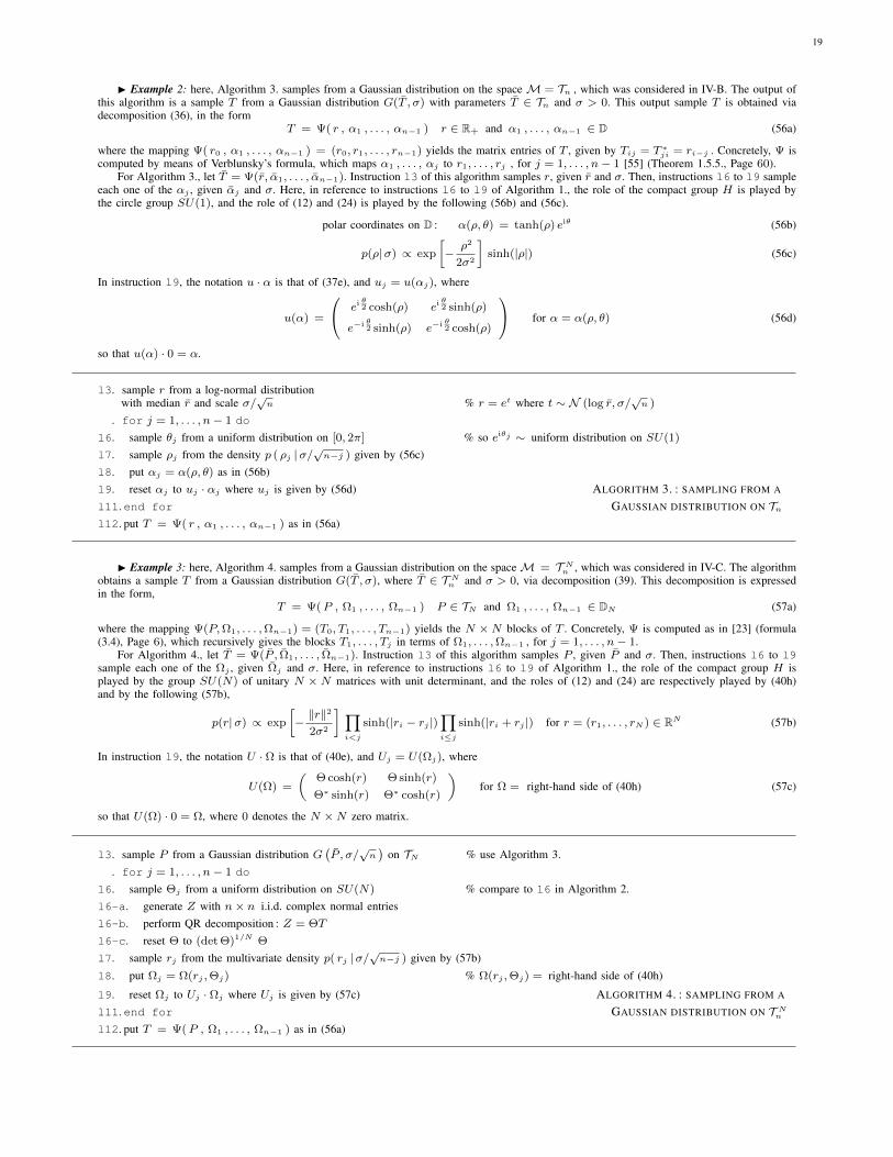
19

I Example 2: here, Algorithm 3. samples from a Gaussian distribution on the space M = Tn , which was considered in IV-B. The output ofthis algorithm is a sample T from a Gaussian distribution G(T , σ) with parameters T ∈ Tn and σ > 0. This output sample T is obtained viadecomposition (36), in the form

T = Ψ( r , α1 , . . . , αn−1 ) r ∈ R+ and α1 , . . . , αn−1 ∈ D (56a)

where the mapping Ψ( r0 , α1 , . . . , αn−1 ) = (r0, r1, . . . , rn−1) yields the matrix entries of T , given by Tij = T ∗ji = ri−j . Concretely, Ψ iscomputed by means of Verblunsky’s formula, which maps α1 , . . . , αj to r1, . . . , rj , for j = 1, . . . , n− 1 [55] (Theorem 1.5.5., Page 60).

For Algorithm 3., let T = Ψ(r, α1, . . . , αn−1). Instruction l3 of this algorithm samples r, given r and σ. Then, instructions l6 to l9 sampleeach one of the αj , given αj and σ. Here, in reference to instructions l6 to l9 of Algorithm 1., the role of the compact group H is played bythe circle group SU(1), and the role of (12) and (24) is played by the following (56b) and (56c).

polar coordinates on D : α(ρ, θ) = tanh(ρ) eiθ (56b)

p(ρ|σ) ∝ exp

[−ρ2

2σ2

]sinh(|ρ|) (56c)

In instruction l9, the notation u · α is that of (37e), and uj = u(αj), where

u(α) =

ei θ2 cosh(ρ) ei θ

2 sinh(ρ)

e−i θ2 sinh(ρ) e−i θ

2 cosh(ρ)

for α = α(ρ, θ) (56d)

so that u(α) · 0 = α.

l3. sample r from a log-normal distributionwith median r and scale σ/

√n % r = et where t ∼ N (log r, σ/

√n )

. for j = 1, . . . , n− 1 do

l6. sample θj from a uniform distribution on [0, 2π] % so eiθj ∼ uniform distribution on SU(1)

l7. sample ρj from the density p ( ρj |σ/√n−j ) given by (56c)

l8. put αj = α(ρ, θ) as in (56b)l9. reset αj to uj · αj where uj is given by (56d) ALGORITHM 3. : SAMPLING FROM A

l11. end for GAUSSIAN DISTRIBUTION ON Tnl12. put T = Ψ( r , α1 , . . . , αn−1 ) as in (56a)

I Example 3: here, Algorithm 4. samples from a Gaussian distribution on the spaceM = T Nn , which was considered in IV-C. The algorithmobtains a sample T from a Gaussian distribution G(T , σ), where T ∈ T Nn and σ > 0, via decomposition (39). This decomposition is expressedin the form,

T = Ψ(P , Ω1 , . . . , Ωn−1 ) P ∈ TN and Ω1 , . . . , Ωn−1 ∈ DN (57a)

where the mapping Ψ(P,Ω1, . . . ,Ωn−1) = (T0, T1, . . . , Tn−1) yields the N ×N blocks of T . Concretely, Ψ is computed as in [23] (formula(3.4), Page 6), which recursively gives the blocks T1, . . . , Tj in terms of Ω1, . . . ,Ωn−1 , for j = 1, . . . , n− 1.

For Algorithm 4., let T = Ψ(P , Ω1, . . . , Ωn−1). Instruction l3 of this algorithm samples P , given P and σ. Then, instructions l6 to l9sample each one of the Ωj , given Ωj and σ. Here, in reference to instructions l6 to l9 of Algorithm 1., the role of the compact group H isplayed by the group SU(N) of unitary N × N matrices with unit determinant, and the roles of (12) and (24) are respectively played by (40h)and by the following (57b),

p(r|σ) ∝ exp

[−‖r‖2

2σ2

] ∏i<j

sinh(|ri − rj |)∏i≤j

sinh(|ri + rj |) for r = (r1, . . . , rN ) ∈ RN (57b)

In instruction l9, the notation U · Ω is that of (40e), and Uj = U(Ωj), where

U(Ω) =

(Θ cosh(r) Θ sinh(r)

Θ∗ sinh(r) Θ∗ cosh(r)

)for Ω = right-hand side of (40h) (57c)

so that U(Ω) · 0 = Ω, where 0 denotes the N ×N zero matrix.

l3. sample P from a Gaussian distribution G(P , σ/

√n)

on TN % use Algorithm 3.. for j = 1, . . . , n− 1 do

l6. sample Θj from a uniform distribution on SU(N) % compare to l6 in Algorithm 2.l6-a. generate Z with n× n i.i.d. complex normal entriesl6-b. perform QR decomposition : Z = ΘT

l6-c. reset Θ to (det Θ)1/N Θ

l7. sample rj from the multivariate density p( rj |σ/√n−j ) given by (57b)

l8. put Ωj = Ω(rj ,Θj) % Ω(rj ,Θj) = right-hand side of (40h)

l9. reset Ωj to Uj · Ωj where Uj is given by (57c) ALGORITHM 4. : SAMPLING FROM A

l11. end for GAUSSIAN DISTRIBUTION ON T Nnl12. put T = Ψ(P , Ω1 , . . . , Ωn−1 ) as in (56a)