Double for Nothing? Experimental Evidence on the Impact of an Unconditional Teacher Salary Increase on Student Performance in Indonesia

Joppe de Ree Karthik Muralidharan Menno Pradhan Halsey Rogers†

15 January 2016

Abstract: How does a large unconditional increase in salary affect employee performance in the public sector? We present the first experimental evidence on this question to date in the context of a unique policy change in Indonesia that led to a permanent doubling of base teacher salaries. Using a large-scale randomized experiment across a representative sample of Indonesian schools that affected more than 3,000 teachers and 80,000 students, we find that the doubling of pay significantly improved teacher satisfaction with their income, reduced the incidence of teachers holding outside jobs, and reduced self-reported financial stress. Nevertheless, after two and three years, the doubling in pay led to no improvements in measures of teacher effort or student learning outcomes, suggesting that the salary increase was a transfer to teachers with no discernible impact on student outcomes. Thus, contrary to the predictions of various efficiency wage models of employee behavior (including gift-exchange, reciprocity, and reduced shirking), as well as those of a model where effort on pro-social tasks is a normal good with a positive income elasticity, we find that unconditional increases in salaries of incumbent teachers had no meaningful positive impact on student learning. JEL Classification: H42, J31, J45, I21, C93, O15 Keywords: efficiency wages, gift exchange, fair wages, reciprocity, teacher salaries, teacher motivation, teacher performance, education quality, Indonesia, field experiments, randomized controlled trials, student learning, personnel economics, public sector labor markets

† Joppe de Ree: World Bank; joppederee@gmail.com Karthik Muralidharan: UC San Diego, NBER, BREAD, J-PAL; kamurali@ucsd.edu Menno Pradhan: University of Amsterdam and VU University Amsterdam; m.p.pradhan@vu.nl Halsey Rogers: World Bank; hrogers@worldbank.org We thank Nageeb Ali, Julie Cullen, Gordon Dahl, Uri Gneezy, Richard Murphy, Derek Neal, Ben Olken, Valerie Ramey, Miguel Urquiola, and several seminar participants for comments. We are grateful to the Indonesian Ministry of Education and Culture for its interest in evaluating its teacher pay reforms, and for supporting this large-scale experiment and data collection. This evaluation would not have been possible without generous financial support from the government of the Kingdom of the Netherlands. The authors are grateful to Dedy Junaedi (and team), Titie Hadiyati (and team), Susiana Iskandar, Amanda Beatty, and Andy Ragatz for their exceptional efforts and support in conducting this evaluation as part of the World Bank BERMUTU project team at various points of time over the course of this project, and to counterparts at the Indonesian Ministry of Education and Culture, including Dr. Baedhowi, Dian Wahyuni, Santi Ambarukmi, Yendri Wirda Burhan, Simon Sili Sabon (and the team at puslitjak), Dhani Nugaan, Bastari, Hari Setiadi, Rahmawati and Yani Sumarno (and the team at puspendik), who supported this experiment and implemented it flawlessly. Over the years, the project also benefited from excellent research assistance of Ai Li Ang, Husnul Rizal and others at the World Bank office in Jakarta. The findings, interpretations, and conclusions expressed in this paper are entirely those of the authors. They do not necessarily represent the views of the National Bureau of Economic Research, the International Bank for Reconstruction and Development/World Bank and its affiliated organizations, or those of the Executive Directors of the World Bank or the governments they represent.

1

1. Introduction

How does a large unconditional increase in salary affect the performance of incumbent

employees in the public sector? While unconditional salary increases do not provide a direct

incentive for increased effort on the job, there are several classes of "efficiency wage" models

that predict improved worker effort in response to such pay increases. These include models of

reciprocity and gift-exchange where employees pay back employers for a wage premium with an

effort premium (Akerlof 1982), and models that posit that employees will shirk less in response

to wage increases because of the increased cost of losing a job with a wage premium (Shapiro

and Stiglitz 1984). A further mechanism highlighted in public-sector contexts is that increasing

the pay of public workers in pro-social tasks like teaching or healthcare provision, would reduce

the incidence of outside jobs and increase time and effort on their primary job, from which they

draw intrinsic utility (UNESCO 2014).

Given the centrality of this question to labor and personnel economics, a large empirical

literature has tried to study the impact of unconditional pay raises on worker effort and

productivity, with varying results (see Esteves-Sorenson and Macera 2015 for a recent review).

However, since it is difficult to exogenously change salaries in real employment settings, most of

the evidence to date has relied on laboratory experiments and short-term field experiments with

researcher-led variation in pay. Thus, despite a large empirical literature on this question, we are

not aware of any experimental study of the impact of a permanent unconditional salary increase

in the context of an existing long-term employment contract. This is a critical gap because

estimates from the existing literature are often used to make inferences about real employment

contracts, which can be problematic (see Levitt and List 2007 for a discussion).1

In this paper, we attempt to bridge this gap by providing experimental evidence on the

intensive-margin impacts on teacher effort and student learning outcomes of a unique policy

change in Indonesia that permanently doubled the base pay of eligible teachers who went

through a certification process.2 Given the large fiscal impact of the policy, teacher access to the

certification program was phased in over 10 years (from 2006 to 2015), with priority in the

1 As they note: "Such inference raises at least two relevant issues. First, is real-world on-the-job effort different in nature from that required in lab tasks? Second, does the effort that we observe in the lab manifest itself over longer time periods?" (Levitt and List 2007) 2 The policy was designed to reward a process of teacher skill upgrading (signaled by "certification") by providing a certification allowance that was equal to the base pay (thereby doubling base pay). However, in practice, the certification mainly consisted of the pay increase (see section 2 for details).

2

certification queue being determined by seniority. Thus, many "eligible" teachers had to wait

several years before being allowed to enter the certification process.

Working closely with the Government of Indonesia, we implemented an experimental design

that allowed all eligible teachers in 120 randomly-selected primary and junior secondary public

schools to immediately access the certification process and the resulting doubling of pay, while

teachers in control schools experienced the "business as usual" access to the certification process

through the gradual phase in over time. The experiment thus created a sharp increase in the

fraction of teachers in treated schools with a permanent doubling of pay during the three years of

our study, which allows us to identify the intensive margin impacts of an unconditional

permanent increase in pay on performance. Further, the experiment featured random assignment

of 120 treatment and 240 control schools within a near-nationally representative sample of 360

schools across 20 districts and all major regions of Indonesia, thereby providing considerable

external validity to our results.3

Given the challenges of implementing a randomized experiment at scale with a national

government, the experiment worked remarkably well with a strong "first stage". It resulted in a

28 percentage point differential increase in the fraction of teachers in treatment schools who had

been certified and paid the salary supplement at the end of two years, and a 23 percentage point

increase at the end of three years (relative to the control group).4 Among the "target" teachers

affected by the experiment (those who were eligible but not certified at the baseline), there was a

54 (and 43) percentage point differential increase in teachers who were certified and paid their

professional allowance at the end of two (and three) years in treatment schools.

The experiment also produced significant impacts on the intermediate mechanisms through

which policymakers hoped that the increase in salary would lead to better education quality. At

the end of two and three years of the experiment, teachers in treated schools had significantly

higher income, were significantly more likely to be satisfied with their income, significantly less

likely report financial stress, and significantly less likely to hold a second job.

3 See Heckman and Smith (1995) for a discussion of the threats to external validity of experiments resulting from site-selection bias in experimental studies. Allcott (2015) provides evidence of such bias. 4 Roughly 20% of teachers in both treatment schools were already certified at baseline, and another 25% of teachers were not eligible for certification in any case (due to not being civil-service teachers or college graduates). It is the remaining 55% of teachers who were "eligible but not certified" at the baseline who are affected by the experiment and it is in this population of teachers that the experiment induces a significant increase in pay. Note that the "first stage" of the experiment will weaken over time in our setting as teachers in the control schools get certified over time (teachers in the control schools were also getting certified, but at a slower rate).

3

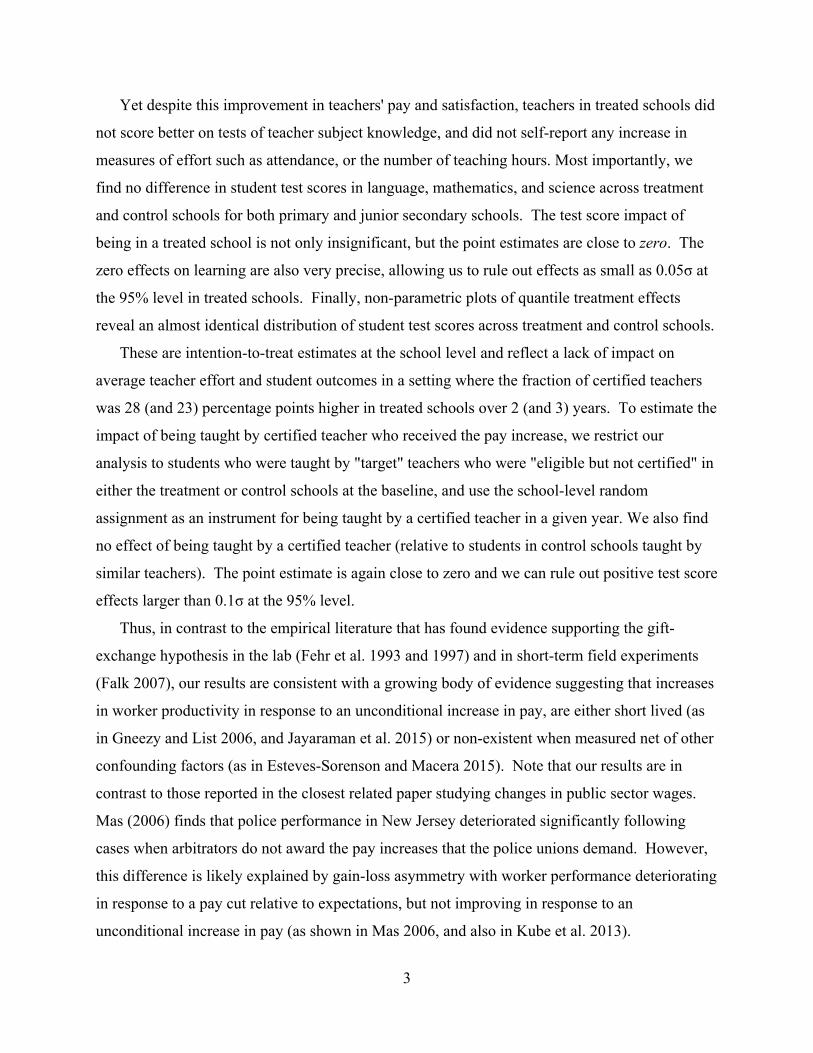
Yet despite this improvement in teachers' pay and satisfaction, teachers in treated schools did

not score better on tests of teacher subject knowledge, and did not self-report any increase in

measures of effort such as attendance, or the number of teaching hours. Most importantly, we

find no difference in student test scores in language, mathematics, and science across treatment

and control schools for both primary and junior secondary schools. The test score impact of

being in a treated school is not only insignificant, but the point estimates are close to zero. The

zero effects on learning are also very precise, allowing us to rule out effects as small as 0.05σ at

the 95% level in treated schools. Finally, non-parametric plots of quantile treatment effects

reveal an almost identical distribution of student test scores across treatment and control schools.

These are intention-to-treat estimates at the school level and reflect a lack of impact on

average teacher effort and student outcomes in a setting where the fraction of certified teachers

was 28 (and 23) percentage points higher in treated schools over 2 (and 3) years. To estimate the

impact of being taught by certified teacher who received the pay increase, we restrict our

analysis to students who were taught by "target" teachers who were "eligible but not certified" in

either the treatment or control schools at the baseline, and use the school-level random

assignment as an instrument for being taught by a certified teacher in a given year. We also find

no effect of being taught by a certified teacher (relative to students in control schools taught by

similar teachers). The point estimate is again close to zero and we can rule out positive test score

effects larger than 0.1σ at the 95% level.

Thus, in contrast to the empirical literature that has found evidence supporting the gift-

exchange hypothesis in the lab (Fehr et al. 1993 and 1997) and in short-term field experiments

(Falk 2007), our results are consistent with a growing body of evidence suggesting that increases

in worker productivity in response to an unconditional increase in pay, are either short lived (as

in Gneezy and List 2006, and Jayaraman et al. 2015) or non-existent when measured net of other

confounding factors (as in Esteves-Sorenson and Macera 2015). Note that our results are in

contrast to those reported in the closest related paper studying changes in public sector wages.

Mas (2006) finds that police performance in New Jersey deteriorated significantly following

cases when arbitrators do not award the pay increases that the police unions demand. However,

this difference is likely explained by gain-loss asymmetry with worker performance deteriorating

in response to a pay cut relative to expectations, but not improving in response to an

unconditional increase in pay (as shown in Mas 2006, and also in Kube et al. 2013).

4

The main contribution of this paper is that it presents the first experimental evidence on the

impact of a permanent wage increase on performance in the context of an existing employment

contract as opposed to researcher-led experiments that have only varied pay in the short run and

have typically been for a new employment contract. It is also (to our knowledge) the largest

experimental study of a wage-increase ever conducted, both in terms of the size of the wage

increase studied and the fiscal commitment represented by the policy (which will cost around

five billion US dollars each year in steady state), and the scale and duration of the experiment

(done in a near-representative sample across a country of 200 million people for three years).

Our results also contribute directly to the literature studying the links between teacher pay

and performance and are consistent with prior evidence finding no correlation between increases

in teacher pay and improved student performance in the US (Hanushek 1986; Betts 1995;

Grogger 1996; Ballou and Podgursky 1997). However, these results have been questioned for not

having adequate exogenous variation in teacher pay, for failing to control for non-wage

compensation and for differences in local labor markets (Loeb and Page 2000), and for being

based on small changes in pay that may be too small to generate detectable impacts on outcomes

(Dolton et al 2011).5 We address all three of these limitations in the existing literature in our

setting.

Our results do not imply that a policy of unconditional salary increases would have no

positive impacts on service delivery in developing countries in the long run. Dal Bo et al (2013)

show that salary increases for public sector jobs in Mexico increased the observable quality of

job applicants, and Ferraz and Finan (2011) find that higher wages for politicians in Brazil led to

improved performance through both a selection channel and an efficiency-wage channel.

However, Dal Bo et al. (2013) are not able to study the impact of higher public sector wages on

performance outcomes or to estimate the cost effectiveness of such a policy, and the results in

Ferraz and Finan (2011) are from a setting where non-performing politicians are more likely to

lose their jobs (where a "reduced shirking" efficiency wage channel is more likely to apply). Our

results complement these by showing that even large unconditional wage increases may yield no

improvement in performance on the intensive margin in a public sector setting of "permanent"

civil-service employment contracts with a low probability of being fired for non-performance.

5 The only study based on a large increase in teacher salaries we are aware of is Ciotti (1998) who studies a large increase in per-child education spending in Kansas City mandated by a court order (a lot of which was spent on teacher salaries), and finds no impact on outcomes. This is, however, a case-study with limited identification.

5

While several education policy reports recommend increasing teacher pay in low-income

countries as a way to improve teacher performance on the intensive margin (UNICEF 2011,

UNESCO 2014), our results suggest that this hypothesis is not supported by the evidence.6 Such

evidence is especially relevant in a public-sector setting, where there is no market test of whether

increasing wages also increases productivity,7 and where policy changes (such as unconditional

increases in salaries) are very difficult to reverse. Thus, policy makers hoping to increase the

quality of government service delivery by increasing salaries across the board need to trade off

the potential benefits on the extensive margin against the large intensive-margin costs of

unconditional increases in public sector pay that may not yield any performance improvement.

The rest of this paper is structured as follows: Section 2 describes the Indonesian education

context and the teacher certification policy, and discusses the theoretical reasons for why the

policy may have improved teacher effort; section 3 describes our experiment (design, validity,

and data collection); section 4 presents results on teacher effort and student outcomes, section 5

interprets our results and discusses policy implications; section 6 concludes.

2. Background, and Policy Change

Indonesia has one of the largest school education systems in the world, serving over 50

million students across 34 provinces and more than 500 districts. The country consists of

thousands of islands spanning over 3000 miles from east to west (Figure 1), making service

delivery quite challenging. Promoting primary education was historically a high policy priority

for Indonesia relative to other developing countries in South Asia and Africa, and Indonesia

achieved high rates of primary school enrollment exceeding 90% by the early 1980s (World

Bank EdStats Database). Nevertheless, the performance of the education system in terms of

student learning outcomes is poor compared to that of many other middle-income countries. For

instance, Indonesian 15-year-olds’ math test scores on the PISA 2012 assessment were

6 Note that our results are based on a large-scale policy experiment, which was not designed to provide a precise test of any one specific theoretical mechanism for why an unconditional salary increase may improve the performance of incumbent workers. However, from a policy perspective, what matters is whether there was an overall effect through any of the plausible mechanisms identified by proponents of higher teacher pay. This is the question that our experiment was designed to answer (see section 3 for a more detailed discussion). 7 In contrast, Henry Ford’s famous "five-dollar workday" led to a similar doubling in wages, but also led to sharp increases in worker productivity (Raff and Summers 1987). Indeed, it is unlikely that Ford would have continued paying high wages if productivity did not go up, whereas the Indonesian government spent billions of dollars on teacher salary increases and has continued doing so each year despite no impact on student learning outcomes.

6

significantly below those of their peers in all but three participating countries, and their scores on

reading and science were similarly low (OECD 2013). On the 2011 TIMSS math assessment,

Indonesian 8th-graders outscored those from only five other countries (Mullis et al. 2012).

Education policy discussions in Indonesia in the years prior to 2005 identified poor teacher

quality and motivation as a key limitation in the performance of the Indonesian education

system. The ambitious education reforms of 2005 aimed explicitly to address this issue and made

a large fiscal commitment to doing so. The highlight of these reforms was the "Teacher Law" of

2005 whereby teachers who met certain eligibility criteria (being a civil-service teacher, and

holding either a four-year university degree, or a high rank in the civil service – typically

obtained through a very long tenure) and who successfully completed a certification process

would receive a "professional allowance" (also referred to as the "certification allowance") equal

to 100% of their base pay (Chang et al. 2014; World Bank 2010).8

The certification process was initially meant to include a high-standards external assessment

of teacher subject knowledge and pedagogical practice, with an extensive skill-upgrading

component for teachers who did not meet these standards that would include up to a year of

additional training and tests. However, teachers’ associations opposed the high-standards

certification exams that were originally planned. Thus, by the time the final law and regulations

were negotiated through the political and policymaking process, the quality-improvement

stipulations had been highly diluted. They were replaced with a much weaker certification

requirement that simply required teachers to submit a portfolio of their teaching materials and

achievements. Even for those who did not pass the portfolio evaluation, just two weeks of

additional training were required to attain certification. Thus in practice the certification process

yielded a doubling of base pay with only a modest hurdle to be surmounted.9

The reform led to a substantial increase in teacher salaries. While pre-reform teacher salaries

in Indonesia were lower than teacher salary benchmarks in other Southeast Asian countries

(which was part of the justification for the policy), teachers were well paid relative to the

distribution of college-graduate salaries in Indonesia both before and after the reform. Using

8 Note that the professional allowance was 100% of base pay, rather than of total pre-certification pay. Teachers often receive other allowances based on location of posting and taking on additional tasks, and so the allowance increased total pay by 80% on average and by 67% for teachers who were eligible for treatment (see Table 5). 9 Very few teachers entering the certification process failed it. For instance, qualitative work showed that “a market for forged certificates and other necessary portfolio items is prevalent.” Further, even those who failed the first attempt were all certified after a two-week training program (World Bank 2010).

7

representative household survey data from the 2012 Indonesian labor force survey (Sakernas,

August 2012), we estimate that the doubling of base pay moved teacher compensation from

around the 50th percentile of the college-graduate salary distribution to the 90th percentile.10

Thus, for eligible teachers the reform significantly improved teachers' financial situation and

hence their ability to focus on their teaching. This very large salary increase was not conditional

on teachers' subsequent effort or effectiveness, but instead depended only on a one-time

determination that the teacher met some certification criteria. Thus, for all practical purposes, the

policy can be considered as having resulted in an unconditional salary increase for eligible

teachers. To the extent that undergoing the certification process actually did increase the human

capital of teachers, our estimates of the impact of certification will be an upper bound on the

intensive-margin impacts of an unconditional increase in pay.

3. Theoretical Considerations

Why should we expect an unconditional salary increase to improve teacher motivation and

effort on the intensive margin? Before discussing the theoretical models that support this idea,

we briefly summarize the policy discourse and documents that informed the policy change.

Before the policy change, its proponents argued that teacher salaries in Indonesia were lower

than those in neighboring middle-income countries (both in absolute terms and relative to per-

capita income), and that low salaries reduced both teachers’ morale and the time they had

available for teaching. A report from early in the reform process that discussed the government’s

justification for the policy change claimed that “[l]ow pay is likely to be one of the main reasons

why teachers perform poorly, have low morale and tend to be poorly qualified” (World Bank

2008). Another stated that “teachers often have a high rate of absenteeism because they take

second jobs to make ends meet. This reality reduces their motivation and effectiveness in the

classroom” (World Bank 2010). After implementation of the Teacher Law, a policy report noted

that “[g]iven the increased remuneration now available to [certified] teachers . . . , it is expected

that there will be some reduction in this (absenteeism) rate” (World Bank 2010).

10 Our estimates are likely to be a lower bound of how well teacher pay ranks among college graduates for several reasons. First, they include only respondents with a positive wage, thus excluding the unemployed. Second, they are based on salaries alone and do not include the generous pensions and benefits for civil-service teachers. Third, they do not account for the certainty value of having much higher levels of employment security relative to the private sector. Consistent with the idea that teacher salaries and benefits were attractive even prior to the reforms, interviews with experts on Indonesian education suggest that teacher quit rates were very low both before and after the reforms.

8

Similar quotes also appear in the global policy literature on teacher quality. UNESCO's

recent "Education for All Global Monitoring Report", claims that "[l]ow salaries reduce teacher

morale and effort" and "teachers often need to take on additional work – sometimes including

private tuition – which can reduce their commitment to their regular teaching jobs and lead to

absenteeism" (UNESCO 2014). Further, qualitative studies of service delivery in developing

countries have highlighted that low pay for public service providers makes it difficult for their

administrative supervisors to demand accountability for performance (e.g., Webb and Valencia

2006 on the case of Peru). A primary school director in Cambodia made this argument

explicitly: "If salaries went up, I could ask them to work harder, give up their second jobs and

spend more time in school planning their work" (VSO 2008). This argument that higher salaries

can lead to greater motivation and better performance appears in the US literature as well; for

example, Hanushek, Kain, and Rivkin (1999) note that in addition to the attraction and retention

channel, "Many influential reports and proposals advocate substantial salary increases as a means

of attracting and retaining more talented teachers in the public schools and encouraging harder

work by current teachers" (emphasis added). A recent US op-ed from the Teacher Salary Project

argued that "Teachers who spend nights and weekends working other jobs cannot possibly

devote the necessary attention to their students or lesson plans."11 Appendix A presents a fuller

list of quotes and extracts from prominent education policy documents in Indonesia and several

countries that claim that increasing teacher pay will increase their motivation and effort.

Thus, this significant policy reform in Indonesia was, at least partly, influenced by the belief,

widely held in the global and local education policy communities, that increasing teacher salaries

would improve teacher effort and student outcomes through intensive-margin channels. Indeed,

the pay increase was widely referred to in policy documents as an "incentive", suggesting an

implicit assumption by policy makers that there would be positive effects on teacher motivation

and effort on the intensive margin (for a recounting of the policymaking process and rationales,

see Chang et al. 2014).12

11 Obtained from https://www.washingtonpost.com/news/answer-sheet/wp/2014/03/25/why-teachers-salaries-should-be-doubled-now/, 13/1/2015 12 The discussion above does not imply that there were no skeptics about the policy in Indonesia (especially in the Ministries of Finance and Planning) and about whether it would be effective at improving education outcomes, especially once the certification program made its way through the political and policymaking process. However, we emphasize the plausible reasons for a positive impact because the policy was implemented despite skepticism from some quarters, and these were among the stated reasons that led to the policy being implemented.

9

In Appendix B, we formalize the different mechanisms underlying the intuitive statements by

practitioners above, and present a simple theoretical sketch of three possible mechanisms for

why teacher effort may increase in response to an unconditional increase in salary and derive

comparative statics. These include: (1) reciprocity and gift exchange in employment contracts

(Akerlof 1982; Fehr and Gachter 2000); (2) a model in which effort on pro-social tasks like

teaching is a normal good with a positive income elasticity, because an increase in salary allows

employees to reduce their hours at outside jobs and frees up time and effort for their primary

teaching job, which gives them greater intrinsic utility (implicit in UNESCO 2014); and (3) a

model where the expected performance of teachers depends on their salary and where non-

pecuniary sanctions or rewards are provided through community and administrative monitoring

based on actual performance relative to expectations (which is the implicit argument made in

Webb and Valencia 2006, and Cotlear 2006).

In principle, the "reduced shirking" channel of efficiency wages (Shapiro-Stiglitz 1984)

should also apply here because there is no theoretical reason for why teachers could not get fired

for low effort. If this were true, an increase in the continuation value of holding their job from

the unconditional salary increase should also induce a reduction in shirking. However, in

practice, it was and is rare for civil-servant teachers to get fired, and we don’t believe that this

channel would apply in our setting as a result. In terms of the model in Appendix B, this would

be equivalent to saying that the "minimum effort" condition (below which employees would get

fired) was not binding before the reform, and would therefore not bind afterwards either (which

is why we do not derive the comparative statics for this channel).

It is important to note that our results are from a large-scale policy experiment that aimed to

improve education quality. Such policy experiments by design are unlikely to yield a precise

theoretical test of any one of the mechanisms listed above. For instance, reciprocity may require

that the "gift" of a higher salary be received from an employer whom the employee interacts with

on a regular basis and towards whom the employee therefore feels an obligation, as opposed to

being received from a "distant" taxpayer. Similarly, the mechanism that depends on reduced

shirking through more effective administrative/ community monitoring may hold only in a

setting where the monitors are able to apply non-pecuniary awards or sanctions that affect

teachers’ behavior. However, policymakers would be less concerned about the precise

mechanism for impact and more interested in whether such an expensive policy had an impact on

10

teacher effort and learning outcomes through any combination of the posited mechanisms above.

This is the question that our study is designed to answer.

4. Experiment Design

4.1. Design, Sampling, and Implementation

Because of the large number of teachers covered, teacher access to the certification process

was phased in for budgetary reasons. The budgetary restrictions meant that only around 10% of

teachers were allowed to go through the certification process each year since implementation of

the certification process began in 2006. Each year, each district was allocated a quota that

indicated how many of its teachers could start the certification process. Once any teacher was in

the process, he or she was practically guaranteed certification, as described above. Other eligible

teachers had to wait in a certification queue, sometimes for several years, with their position in

the queue determined by their seniority.

Our experimental design takes advantage of the phase-in procedure for teacher access to the

certification process. Rather than having teachers wait in the certification queue, the intervention

aimed to allow all eligible but not yet certified teachers (we define these as "target" teachers) in

treatment schools to immediately access the certification process at the start of the experiment (in

2009). Note that the experiment did not change any of the requirements of certification specified

in the law and regulations, but simply allowed otherwise eligible teachers in treatment schools to

enter the certification process early, rather than having to wait for a few more years. The

experimental protocol was implemented in close collaboration with the Ministry of National

Education of the Government of Indonesia, where senior officials were committed to conducting

a high-quality impact evaluation, and provided exemplary support in implementation.

We first identified a near-representative sample of 360 schools across 20 districts of

Indonesia to comprise the universe of the study. We started with the 2006 national teacher

census, which covered roughly 1,600,000 public primary and junior-secondary teachers across

454 districts. Districts that were too small, were too dangerous to visit, or that were included in a

parallel randomized evaluation were excluded13, leaving us with 383 districts in the sampling

13 Note that the district sampling for the two parallel sets of randomized evaluations were conducted using the same procedures, and so the 20 districts dropped on account of not wanting spillovers between the studies were also a representative sample. However, the second study ended up not being implemented. Note also that the districts dropped for access and safety reasons had much lower population on average.

11

frame. These represented nearly 85% of the districts and over 90% of the population of

Indonesia. From these, we randomly sampled 20 districts, stratified across the five major regions

of the country, with more districts assigned to regions with a larger population. The list of

districts sampled and the strata they represent are presented in Table A.1. A map of the sampled

districts and their representativeness is presented in Figure 1.14

Within each district, we stratified schools by the number of teachers, and sampled 12 primary

and 6 junior secondary schools (stratified by school size).15 Thus, the study universe consisted of

a near-representative sample of 240 primary and 120 junior secondary schools across 20 districts

of Indonesia. 80 primary and 40 junior secondary schools were then randomly assigned to

"treatment" status, while the other 160 primary and 80 junior secondary schools were assigned to

a "business as usual" control group. Just like the sampling of schools, the randomization was

also stratified by district, school-type, and school size, and thus the design was identical across

districts, with each district being a microcosm of the overall study.16

Teachers in treatment schools, who were eligible for certification but not yet certified,

received a personal letter from the Ministry of National Education informing them that they had

been granted immediate access to the certification process. To ensure that other teachers would

have no incentive to transfer to treatment schools, only teachers who worked in the treatment

schools at the start of the experiment were eligible for this immediate access. The budget for the

extra certification "slots" created for the experimental study was provided through supplementary

funds from the National Government, and these slots were provided to districts over and above

their regular certification quota.

14 The five major regions of Indonesia and the number of districts sampled in each of them (roughly proportional to population) include Java (10), Sumatra (5), Sulawesi (2), Eastern Indonesia (2), and Kalimantan (1). As the scale in Figure 1 shows, the East-West distance spanned by Indonesia is greater than that of the continental United States, and the design imposed considerable logistical complexity. However, the resulting random assignment in a near-representative sample of schools provides greater external validity to our results. 15 We dropped the strata comprising schools with very large and very small number of teachers. If schools were too large, it would not have been feasible to test all the students in the school during the time that the enumerators would have in the school. If they were too small, they would not provide adequate power. Note that primary schools cover grades 1-6, while junior secondary schools cover grades 7-9. We find no evidence of heterogeneous effects as a function of the number of teachers in the school, and so our results are likely to be representative of all schools, even though the smallest and largest ones were not in the study universe. 16 Specifically, each of the 20 districts had 6 treatment schools (2 junior secondary and 4 primary) and 12 control schools (4 junior secondary and 8 primary). Schools were stratified into "triplets" based on size, and one school in each triplet was assigned to treatment status. Note that the intervention was expensive and thus, optimal sample allocation to maximize power yielded a larger control group than treatment group.

12

The research design did not create any other change in the schools besides the additional

quota allocation to treatment schools and the personalized letter sent to the "target" teachers

(who were eligible but not certified at the start of the 2009-2010 academic year). The teachers in

control schools continued business as usual, and those who were eligible but not certified at the

start of the study progressed through the certification process at the same rate as the rest of the

country. Thus, our identifying variation comes from the sharp increase in the fraction of

certified teachers in the treatment schools during the experiment, contrasted with the gradual,

business-as-usual increase in the control schools.

The possibilities of spillovers to other schools were minimized by making sure that there was

no public announcement of the additional quota: the eligibility for certification was

communicated to teachers only by the personalized letter that they received from the

Government. Further, within the treatment schools, the teachers who did not receive the

certification letter were those who were not eligible for certification in any case (by virtue of not

being a college graduate or a civil-service teacher); as a result, the experiment is less likely to

have engendered resentment among non-target teachers in the school than in settings where the

pay increases might have been seen as arbitrary. Thus, by conducting our study in a setting

where the pay increases were in line with pre-announced policy criteria, we minimize the extent

to which the intervention may be considered ad hoc or unsustainable.

4.2. Project Timeline and Data

The school year in Indonesia runs from July to May, and the experiment was carried out over

three school years from 2009-10 to 2011-12 (and we refer to these three years as Y1, Y2, and Y3

in the paper). The sampling and randomization of schools were conducted during the school

holidays before Y1, and the government sent letters to eligible uncertified teachers announcing

their access to the certification process at the start of the school year. The certification process

(including preparing and submitting the application and teaching portfolio, having this evaluated,

and receiving the certification) typically took one full school year, and teachers typically got

"certified" by the end of Y1, and started receiving their certification allowance (equal to 100% of

base pay) at the start of Y2.

We carried out three waves of data collection, during which we interviewed head-teachers,

teachers, and students, and we conducted independent tests of both teacher knowledge and

student learning outcomes. The first wave was a baseline collected in October 2009, which we

13

refer to as Y0. The baseline was deliberately conducted a few months into the school year (after

the certification eligibility letters were sent to teachers in treatment schools) so that we could

verify through interviews of the teachers that they had in fact received these letters and entered

the certification process. The second wave of data was collected in April-May 2011 at the end of

2 years of the project (Y2), and the third wave was collected in April-May 2012 at the end of 3

years (Y3).17 Figure 2 shows the project timeline for the intervention and data collection.

We collected data on school facilities, finances, and other school-level data from head-

teacher interviews. Teacher interviews included questions on demographics, experience, pay,

outside jobs, income (from teaching and other sources), and job satisfaction. We used a

combination of school and teacher interviews to map teachers to specific classrooms and subjects

(which will not be needed for the school-level ITT estimates, but will be needed for the IV

estimates of the impact of being taught by a certified teacher). Students in all schools were

tested on multiple choice tests of math, science, and Indonesian, and students in junior secondary

schools were also tested in English. The tests also included a short demographic survey to

collect basic information on household assets from students.

4.3 Validity of Experimental Design

The randomization was successful in ensuring that treatment and control schools were similar

prior to the experiment. There was no significant difference between treatment and control

schools on school-level variables such as the number of students, teachers, or student teacher

ratio (Table 1- Panel A). There were also no significant differences in student test scores across

treatment and control schools on test scores in any subject (math, science, Indonesian, or

English) or in an index of household assets (Table 1 - Panel B).18

Similarly, we see no significant difference in teacher characteristics across treatment and

control schools either. There were no significant differences on teacher-level variables including

teachers’ own test scores, their certification status, their base pay, or the incidence of holding an

outside job (Table 2: Columns 1-3). The only difference (which is as expected) is that teachers

17 Since the certification process took one year, the first year in which target teachers in treatment schools would have received the additional allowance was the second year of the project. We therefore felt that it was highly unlikely that there would be any impact at the end of Y1 (since teachers in treatment schools would not have received any additional payments at this point). Thus, given the high costs of surveys across the Indonesian islands, we did not collect data at the end of Y1. 18 Note that the randomization (and communication to "target" teachers was carried out before the baseline survey) and hence the randomization could not be balanced ex ante on these variables. Thus, it is reassuring to see that treatment and control schools were balanced on observables.

14

in treatment schools are 32 percentage points more likely to have entered the certification

quota—a difference that confirms that the intervention successfully led to many more teachers in

treatment schools getting access to the certification process.

We see the impact of the treatment even more clearly in Table 2: Columns 4-6, which are

restricted to the "target" teachers who were "eligible but not certified" in either the treatment or

control schools at the start of the study. In this group, 72.6% of teachers in treatment schools

were in the certification quota, whereas in the control schools, the rate was only 18.5%

(indicating the rate at which eligible but uncertified teachers would have gotten certified in the

absence of the experiment). All other teacher characteristics are identical on average, as

expected. The focus of our analysis will be on school-level ITT estimates (using the sample of

all teachers as shown in columns 1-3), and on IV estimates of being taught by a certified teacher

(using the sample of "target" teachers as shown in columns 4-6).19

In addition to balance on initial characteristics across treatment and control schools, we also

test for differential attrition and entry of students over the period of the study. Table A.3 shows

the different cohorts in our study, the years in which they were tested, and which cohorts are in

our estimation sample at different points of the study. We find that there is no differential

attrition among students who were in our baseline test and who continue to be in our estimation

sample over time (Table A.4 – Panel A), and also that there is no difference in attrition rates

across treatment and control groups as a function of baseline test scores. We also find that the

treatment does not seem to have induced any compositional changes in incoming student cohorts

over time (Table A.5).

5. Results

5.1 First-Stage

The time path of the fraction of teachers in treatment and control schools who had entered the

certification process over the three years of the study is shown in Figure 3. Three points are

noteworthy. First, there was no difference in the rate of teacher certification between treatment

and control schools before the start of the experiment in 2009. Second, the intervention

introduced a sharp increase in the fraction of teachers admitted to the certification process in

treatment schools in 2009, even as the trend in control schools remained constant. Third, the gap

19 We also show balance for teachers who were already certified and for those who were not eligible for certification (Table A.2). Teacher characteristics continue to be balanced in both these sub-groups as well.

15

in fraction of admitted teachers narrowed over time, as the eligible teachers in the control schools

gained access to the certification process at a "business as usual" rate. Thus, the difference in the

fraction of teachers admitted to the certification process across treatment and control schools is

higher at the time of the baseline survey than at the end of Y2 and Y3.20

As described earlier, teachers entered the certification process at the start of each school year,

completed the process over the course of the year, got certified by the end of the year, and started

receiving their payments at the start of the next year. Thus, at the time of the baseline there was

no difference between treatment and control schools in the fraction of teachers who were

certified or who had received the extra certification allowance. However, there was a sharp

increase in both of these indicators at the end of Y2 and Y3 (Figure 4).

Table 3 - Panel A shows the differences in Figures 3 and 4, along with tests of equality. In

the first year, the share of teachers in treatment schools who had entered the certification process

was 32 percentage points higher (or more than double) than that in the control group, while there

was not yet any difference in the fraction certified or paid the certification allowance. At the end

of Y2 and Y3, the difference in the fraction of teachers who had entered the certification process

falls to 17 and 8 percentage points respectively (since the control schools "catch up" over time).

At the end of Y2 (Y3), the fraction of teachers in treatment schools who report being certified is

23 (14) percentage points higher, and the fraction who report being paid the certification

allowance is 28 (23) percentage points higher.

Note that the difference in fraction of teachers who are paid their certification allowance is

higher than the difference in the fraction who are certified (in both Y2 and Y3). This result is

expected: many eligible teachers in the control schools would have entered the certification

process at the start of Y2 and Y3 and then been certified only at the end of Y2 and Y3

respectively, but would only have started getting paid their allowances at the start of the next

school year. These teachers will therefore report being certified but will not yet have started

getting paid their allowance at the time of the Y2 and Y3 surveys, respectively. On the other

hand, teachers in treatment schools who gained access to the certification process at the start of

Y1 will have completed getting certified by the end of Y1, and started getting paid their

20 Some of the teachers who were not eligible for certification at the start of the study (typically because they lacked college degrees) do become eligible over time as they complete the eligibility requirement. However, teachers who become eligible for certification in treatment schools in later years did not receive accelerated access.

16

allowances in Y2.21 Since most of the posited mechanisms by which the pay increase would be

expected to improve teacher effort and student outcomes are based on teachers actually receiving

the extra pay, the most relevant metric of the "effective difference" between treatment and

control schools for our study is the difference in the fraction of teachers who have been "paid

their certification allowance".

In addition to school-level average differences, we also show the impact of being in a treated

school for each of the three categories of teachers: teachers who were "eligible but not certified"

and were the "targets" of the intervention, teachers who were "already certified," and teachers

who were "not eligible" (because they did not have a college degree or were not civil service

teachers). As expected, we see most of the differences in the school-level averages being driven

by the target teachers, for whom there is a 54 percentage point increase in the probability of

entering the certification process. At the end of Y2 (Y3), they are 42 (24) percentage points

more likely to be certified, and 54 (43) percentage points more likely to have been paid their

certification allowance (Table 3 - Panel B). By definition, there is no impact on teachers who

were already certified (Table 3 - Panel C).

For the teachers who were not eligible under the official norms of the Ministry of National

Education, we do see a very small impact of being in a treated school, with a 2 percentage point

increase in the fraction of teachers who are certified and paid at the end of Y2 and Y3 (Table 3 –

Panel D). These most likely reflect cases where teachers may have possessed alternative

credentials that were acceptable as a basis for certification eligibility in lieu of a college degree

(which is the basis on which we classified the eligibility status of teachers), which could have

made them eligible for certification despite our classifying them as ineligible. 22 Since we focus

21 Thus, the difference between treatment and control groups across measures reflects variation in the year of entry into the certification process and the time lag in the process. Once we control for year of entry into certification, the difference between treatment and control schools in the fraction of teachers who are certified and the fraction who are "certified and paid" is the same. 22 Note that some teachers who were not eligible for certification at the start of the experiment do become eligible over time as they complete the eligibility requirement (typically obtaining the equivalent of a college degree). We see that around 19% of these teachers had entered the certification process, around 8% of them had gotten certified, and around 2% had received certification allowances by the end of Y3 (Table 3 – Panel D). This is why the number of teachers entering the certification process grows over time even in the treatment schools (Figure 3). However, the experiment only provided accelerated access to certification to "eligible but not certified" teachers in the treatment schools at the start of the study. This was a one-time process communicated to teachers by an individual letter from the Ministry of National Education with no public announcement. Thus, eligible teachers who may have transferred to the treatment schools later were not provided accelerated access. which is the likely explanation for the insignificant difference in certification rates across treatment and control schools among this group of teachers at the end of Y3.

17

on school-level intention-to-treat effects, the breakdown in Table 3 – Panels B to D is presented

mainly to provide clarity on how the experiment affected the three types of teachers.

5.2 Teacher-level Outcomes

We find that the accelerated access to the certification process and the additional allowance

had several positive impacts on teachers that persisted both two and three years into the

experimental study. At the end of Y2 (Y3), teachers in treatment schools received 96% (54%)

more certification pay and 14% (10%) more total pay compared to those in control schools. They

were also 14% (12%) more likely to report being satisfied with their total income, 18% (16%)

less likely to report facing financial problems and stress, and 18% (18%) less likely to be holding

a second job (Table 4 – columns 1-6).23

As we would expect, the impacts are considerably stronger within the universe of "target"

teachers. "Target" teachers in teachers in treatment schools received 269% (97%) more

certification pay and 25% (18%) more total pay compared to those in control schools. Note that

the certification allowance was 100% of base pay for teachers, but that in practice, the increase

over their total pre-certification pay was around 63-67% because the total pay (prior to

certification) would have included a few allowances in addition to their base pay.24 "Target"

teachers in treatment schools were also 29% (23%) more likely to report being satisfied with

their total income, 29% (30%) less likely to report facing financial problems and stress, and 17%

(20%) less likely to be holding a second job at the end of Y2 (Y3) (Table 4 – Columns 7-12).

The corresponding changes for teachers who were already certified and for those not eligible for

certification are shown in Table A.6.

Since eligible teachers in control schools would also become eligible for certification over

time, our experiment did not induce a doubling in permanent income. Rather, it accelerated a

permanent doubling of base pay, and increased lifetime income for target teachers by 2 to 3 years

23 These figures are presented in percentage changes relative to the mean in the control group. The tables present the changes in percentage points 24 It is easy to back this out from the figures in Tables 3 and 4. In the sample with all teachers, we see in Table 3 that 55.4% of teachers in the treatment group had been paid the certification allowance in Y2, and see in Table 4 that the mean certification pay received by this group was 1.111million IDR (million Indonesian Rupiah). Thus, average certification pay conditional on receiving it was 1.111M/0.554, which is 2.01 million IDR. This is, as it should be, a 100% increase over the mean base pay of 2.02 million IDR. Base pay plus allowances equals 2.79 million IDR, so certification pay was 67% of pre certification pay (2.01/2.97). The calculation can also be done with the "target" teachers, where we see that the average certification pay conditional on receiving it in Y2 was 1.4M/0.72, which is similar at 1.94 million IDR. But since other allowances for civil service teachers were higher, the pre-certification pay for the "target" teachers was 3.1M. Thus, certified teachers received a 63% increase (1.94/3.1) in their total pay.

18

of base pay. Further, while eligible teachers in control schools may have been able to anticipate

their future increase in income, credit constraints may have limited the extent to which they

could borrow against future income. Thus, the effects we report above on increased job

satisfaction, reduced financial stress, and reduced outside jobs should be interpreted as the result

of the increase in 2 to 3 years of permanent income as well as the liquidity effects of actually

receiving the extra income on hand.

Overall, the teacher pay increase induced by our experiment was successful in achieving the

stated objectives of the certification policy regarding teachers' financial situation, job

satisfaction, and ability to better focus on teaching by reducing the need to hold outside jobs.

However, we find no evidence to suggest that teachers in treatment schools put in greater effort

in response to this pay increase. We find no difference between treatment and control schools on

teacher test scores or the likelihood of pursuing further education, suggesting that teachers did

not use the extra time available for their primary teaching job to upgrade their skills in any

meaningful way. We also find no difference in self-reported teaching hours per week or in

absence rates, suggesting that teacher effort was also unchanged. These results hold for both the

overall sample of teachers and the sample that is restricted to "target" teachers, who received an

even larger increase in pay.

Nevertheless, as per the theoretical mechanisms described in section 3, it is possible that the

reduced financial stress, reduced incidence of second jobs, and increased motivation could have

led to an improvement in teacher effectiveness as measured by student learning outcomes; we

test this possibility in the next section.

5.3 Student Outcomes

5.3.1 Intention to Treat (ITT) Estimates

Since the randomization was conducted at the school level, we first present school-level

intention-to-treat estimates of the impact on student learning outcomes of being in a school that

had a sharp increase in the fraction of certified teachers who had received a large unconditional

increase in pay. Our main estimating equation takes the form:

∙ ijksT ∙ ∙ ∙ (1)

The dependent variable of interest is ijksdT , which is the normalized test score of student i on

subject s, where j, k, denote the grade, and school respectively. )( 0YT indicates the baseline tests,

19

while )( nYT indicates a test at period Y1 and Y2. Including the normalized baseline test score

improves efficiency, due to the autocorrelation between test scores across multiple periods.25

We also include a set of stratum fixed effects ( , to absorb geographic variation and increase

efficiency, and to account for the stratification of the randomization (which was done within

district-level "triplets" of schools as described in section 3.1). Finally, we also include the mean

normalized baseline test scores across all students in the school in the concerned grade and

subject ( ijksT ), which further increases efficiency (Altonji and Mansfield 2014). The main

estimate of interest is , which provides an unbiased estimate of the impact of being in a

"Treatment" school (the intent-to-treat or ITT estimate) since schools were assigned to

"Treatment" status by lottery.

We present these ITT results in Table 5—first combined across school types (columns 1-5),

and then separated by primary schools (columns 6-10) and junior secondary schools (columns

10-14). We present results individually for each subject, and also pooled across subjects, and

present results separately by Y2 and Y3 (Panel A and B respectively). Overall, we find no

evidence that students in treatment schools (which experience a significant increase in the

fraction of certified teachers) scored any better than those in control schools. Not a single effect

(in any subject, in either type of school, or at either of the two time periods) is significantly

different from zero, and the pooled effects across subjects and school types have a point estimate

of 0.00σ at the end of Y2 and 0.01σ at the end of Y3. These zero effects are very precisely

estimated with standard errors of 0.025σ, which provides us adequate power to detect effects as

low as 0.05σ at the 5% level. Thus, not only are the point estimates close to zero, but we can

also reject effect sizes greater than 0.042σ at the end of Y2 and effect sizes greater than 0.061σ at

the end of Y3.

Figure 5 presents quantile treatment effects of being in a treatment school, by plotting student

test scores at each percentile of the control and treatment school test score distribution after Y2

and Y3 (left hand side plots). We see that the treatment effects are not only zero on average, but

close to zero at every part of the test score distribution. On the right-hand side, we plot the

25 As we show in Table A.3, some of the cohorts included in our analysis did not have a baseline test. We set the normalized baseline score to zero for these students (similarly for students who may have been absent at the time of the baseline test but are present in the Y2 and Y3 tests) and include a dummy variable in equation (1) that takes the value 1 when the lagged test score is missing and 0 when it is present. We also allow the coefficient on the lagged test score to vary by grade.

20

corresponding "first stage" quantile plots where we show the number of years that a student at

each quantile of the test-score distribution spent with a certified teacher in a treatment and

control school. The figure makes clear that students at every percentile of the test-score

distribution after Y2 and Y3 experienced a significant increase in their exposure to a certified

teacher, but that nevertheless there was no impact on learning outcomes.

One issue in interpreting our school-level ITT estimates is that it is possible that the

estimated zero effects result from a combination of positive effects on students taught by

teachers who were "targets" of the experimental intervention (who may be motivated to increase

effort by the pay raise) and negative effects on students taught by "non-target" teachers

(especially those who were not eligible for certification), who may have withdrawn effort in

response to the perceived "unfairness" of not receiving the certification allowance.26 We test for

this possibility by decomposing the composite results shown in Table 5 by students taught by

"target" teachers and those taught by non-target teachers (across treatment and control schools)

and present the results in Table 6.

For the Y2 data, we simply consider whether a student was taught by a target teacher in Y2

(since none of the teachers affected by the treatment would have been paid the certification

allowance in Y1), and find no significant difference in the outcomes of these students across

treatment and control schools in any subject or in either type of school (Table 6 - Panel A). For

the Y3 data, we consider the four possible combinations of teacher type that a student could have

had in Y2 and Y3 (target – target; target – non-target; non-target – target; and non-target – non-

target) and again find no significant different in test-score outcomes across these categories

between treatment and control schools. When we focus on the most extreme comparison of

students in treatment schools, by comparing those who were taught by a target teacher in both

Y2 and Y3 with those taught by a non-target teacher in both Y2 and Y3, we still find no evidence

that the former did better (if anything, the point estimates on those taught by non-target teachers

in both years are slightly higher for all subjects).

5.3.2 Instrumental Variable (IV) Estimates

The ITT estimates presented above are at the school level, and are based on a 28 (23)

percentage point increase in the fraction of "certified and paid" teachers in the treatment schools

26 As described earlier, the design of the experiment would have mitigated against this possibility, because the experiment did not change any of the certification norms stipulated in the law, and thus there is no reason for non-eligible teachers to feel such resentment. But we still test for this possibility.

21

at the end of Y2 (Y3). To estimate the direct impact of being taught by a certified teacher, we

restrict ourselves to the students who were taught by a "target" teacher and instrument for being

taught by a certified teacher using the random assignment of treatment across schools.

Specifically, we aim to estimate:

∙ ijksT ∙ ∙ ∙ (2a)

∙ ijksT ∙ ϒ ∙

∙ (2b)

where the coefficient of interest is , which estimates the impact on student test-scores for each

year of being taught by a Certified teacher (with the additional pay), and the rest of the variables

are defined as in Eq. (1).

One technical consideration in estimating Eq. (2b) is the issue of test-score decay (or

incomplete persistence) over time. Estimates from several settings suggest that there is

considerable annual decay in test scores, with the persistence parameter ϒ(estimated as the

coefficient on the lagged test score in a standard value-added model) typically being around 0.5

(Andrabi et al. 2013, Muralidharan 2012). Since it is not possible to jointly estimate the

persistence parameter and an unbiased experimental treatment effect at the same time (see

Andrabi et al. 2013 and Muralidharan 2012 for further discussion), we estimate Eq. (2b) for

different values of ϒ and present estimates of , along with standard errors for a range of values

of ϒ in Table 7. The estimates with ϒ = 0 correspond to complete decay of any test score gains

in a year by the end of the next year, while those with ϒ = 1 correspond to complete persistence.

Based on several prior studies, our preferred estimates assume ϒ = 0.5.

The main threat to interpreting these estimates as the annual impact of being taught by a

certified teacher (at different persistence rates) is the possibility of endogenous re-assignment of

certified teachers within treatment schools to potentially weaker students. We test for this in

Table A.7 and find that there is no significant difference in the characteristics of students

assigned to target teachers across treatment and control schools during either the second and

third year of the project (Table A.7 – Panel A). We also find no difference in the probability of

22

students being assigned to a target teacher as a function of whether they are above or below the

median asset ownership.27

Thus, the results in Table 7 use the experiment to credibly show that the causal impact on

student test score gains of being taught by a certified teacher is close to zero. We present IV

estimates for both the full sample of students, as well as for the sample of students taught by

target teachers (which will give us more precise IV estimates, since the first-stage is higher in

this case). Focusing on students who were taught by target teachers, we can reject a positive

effect greater than 0.065σ at the 95% level in the Y2 data. In the Y3 data, our preferred estimate

is the one where the sample includes students who were taught by a target teacher in either Y2 or

Y3, and we find that we can reject a positive effect greater than 0.1σ at the 95% level.28

Finally, we examine heterogeneity of treatment effects as a function of several school-level

characteristics, including the fraction of all teachers who were target teachers, the total number

of target teachers, average student affluence, several measures of school size, as well as mean

baseline test scores in the school. We find no evidence of heterogeneous effects by any of these

characteristics (Table 8). Thus, we find that doubling teacher base pay had almost no impact on

improving student test scores, either in aggregate or in any subset of the data. This finding

suggests that the various posited mechanisms for why such a pay increase may have a positive

impact on student learning (as described in Section 3) were not empirically salient in this setting.

6. Cost Effectiveness and Policy Implications

Viewed as a program to improve learning outcomes in developing countries, increasing

teacher salaries across the board as was done in Indonesia is clearly very expensive. Of course,

most of the costs of the program do not represent a social cost, because the salary increase

mostly represents a transfer to teachers. The actual social cost of the program would be the

deadweight loss of raising tax revenue, and the cost of implementing the certification program.

However, developing countries often face hard budget constraints because of limited ability to

run deficits and the cost of ineffective public spending should also include the opportunity cost 27 Note that we test for differential assignment of students to target teachers as a function of the household asset index (as opposed to the baseline test scores) because we do not have baseline test scores for many of the cohorts in our final estimation sample. As Table A.3 shows, we do not have baseline test scores for any cohort in Y3 for junior secondary schools because junior secondary school only lasts for 3 years. 28 We also show the ITT effects for each estimation sample in Table 7 to enable a clear comparison between ITT and IV estimates. These are almost identical because we find very little difference in outcomes across students taught by target and non-target teachers (as seen in Table 6).

23

of potentially higher-return public spending that was crowded out.29 To simplify our analysis,

we limit the use of this "opportunity cost" framework to education. We assume that there is a

fixed education budget, and compare this program to other education interventions that may have

been possible to implement with the same resources.

For this experiment, the additional salary costs due to accelerated certification were about 66

US dollars per student in the treatment schools.30 The cost of implementing the certification

program should also be added to this figure, but we have too little information to make a credible

estimate. Doing so would require assessing the time costs of teachers, assessors, and trainers--

who have to prepare and assess portfolios and possibly attend training--as well as other

administrative costs. But even without including those costs, it is clear that other salary-related

interventions have been able to achieve substantial positive effects on learning at much lower

cost. For instance, a multi-year experimental program providing performance-based incentive

pay to teachers in India (Muralidharan and Sundararaman 2011) had additional yearly salary

costs of only about 4 US dollars per student (including implementation costs)31, yet it achieved

student learning gains of 0.27σ and 0.17σ in math and language respectively. Over a 5-year

period, the performance- pay experiment yielded gains of 0.54σ and 0.35σ in math and language

for a cohort exposed to the performance-pay intervention for five years (Muralidharan 2012).

These calculations focus only on the intensive margin, and it is possible that education

quality in Indonesia could improve over time as a result of higher-quality professionals entering

the teaching profession.32 However, there are three considerations to keep in mind while

weighing this extensive-margin argument.

29 In principle, governments should be able to borrow to finance any project that has a higher rate of return than the cost of borrowing. In practice, financial markets find it difficult to evaluate the quality of public spending and impose a sovereign risk interest rate penalty when fiscal deficits exceed a threshold. Thus, ineffective public spending will typically reduce the fiscal space for more productive public investments. 30 Costs were calculated by adding up impacts on monthly certification allowance in Y2 and Y3 (0.543+0.476=1.019mln IDR, Table 4, all teachers), multiplying this by 12 and the average number of teachers (9.3, Table 1) and dividing by the average number of children in a school (190, Table 1), using a 9000 IDR/US dollar exchange rate from the duration of the experiment was 2009-2012. 31 Incentive treatments cost up to Rupees 10,000 per school. Per student costs obtained by dividing by average student in school (113), and using an exchange rate of 44 Rupees to the dollar (in the years of the experiment 2005-2007), yielding a cost of 2 US Dollars per student. The authors conservatively estimate the cost of implementing the program as equal to the costs of the bonuses, and so including the implementation cost would double the per-child cost to 4 USD per student, which is the figure we use. 32 Chang et al. (2014) provide some suggestive evidence that the quality of applicants to education faculties of some tertiary institutions has risen. It is too early to tell, however, whether this has meant higher quality of new entrants into the teaching force, in part because there has not been a good measure of quality of entrants. At the system-wide level, if there have been improvements in quality of new teachers, it has not yet increased scores on international

24

First, even if the policy led to an improvement in the quality of teachers entering the

profession, there would still be a very large intensive margin cost of the policy. For instance, if

we assume a uniform distribution of civil-service teachers between ages 30 and 60, the intensive-

margin cost of a policy of doubling teacher pay across the board would be equal to 15 years of

the annual teacher wage bill in Indonesia. Discounting at 5% (assuming conservatively that

nominal wages increase with inflation, and not with growth rates), the present discounted cost

would be over 10 years of the annual teacher wage bill. Since teacher salaries comprise over

10% of the annual Indonesian government budget, the present discounted intensive margin cost

of the policy is more than 100% of the annual government budget. Since it is politically

challenging for higher salaries to only apply to new entrants, it may be difficult to avoid the large

intensive margin costs of an unconditional across the board pay increase.

Second, even if such an increase raises the general ability of new entrants into the teaching

profession, it is not obvious that this would improve social welfare because that talent would be

getting displaced from other sectors in the economy. While it is possible that the social returns of

attracting more talented individuals to teaching may be higher than the costs to the sector they

are displaced from, there is no evidence that this is the case. Further, since public-sector

management quality and productivity is typically lower than that of the private sector (Bloom

and Van Reenen 2010) it is possible that higher-quality human capital may be less productive in

the public sector and that such a displacement may reduce aggregate output.33

Third and finally, an alternative policy that connected at least some of the pay increases to

performance is likely to be more effective on the extensive margin as well, since increasing the

spread of worker pay to more closely reflect their productivity is likely to also be more effective

at attracting higher-ability candidates than an across-the-board increase in salaries on a

compressed schedule that is not linked to performance (Lazear 2000). In the context of

education, Muralidharan and Sundararaman (2011b) find that teachers who are ex-ante more

willing to accept a mean-preserving spread in pay linked to their performance are the ones who

are more effective ex post, suggesting that a similar argument may apply for teachers in

Indonesia as well.

assessments of lower-secondary students. Indonesia’s average PISA scores in math and science fell between 2006 and 2012, while reading scores were stagnant, and average TIMSS scores fell substantially between 2007 and 2011. 33 For instance, Schuendeln and Playforth (2014) present evidence from India suggesting that educated workers prefer to join the government sector (which has high wages and high private returns) even though the social returns of the government sector are low.

25

Thus, while increasing teacher compensation across the board may have some positive long-

term effects on education quality by increasing teacher quality, our results and the discussion

above suggest that there may be much more cost-effective ways of doing so.

7. Discussion and Conclusion

This paper has offered new evidence on a key question in labor and personnel economics:

How does a large, unconditional increase in salary affect employee job performance on the

intensive margin? Answering this question is especially important in public sector contexts

where arguments are often made that unconditional increases in salary will improve the

performance of incumbent workers. However, there is not only a paucity of evidence on this

question, but there is also no market test of whether this is true in practice, and so it is possible

for policies to be misguided for a long time without a credible feedback mechanism on the

effectiveness of expensive policies such as unconditional increases in employee pay.

This paper contributes to answering this question with a large-scale randomized experiment

in the context of a unique policy change in Indonesia that led to a permanent doubling of base

teacher salaries. The experiment was implemented successfully, and led to a large increase in

teacher incomes in treated schools. We find that the experiment also substantially improved the

intermediate variables through which policymakers hoped that the increase in salary would lead

to better education quality: teachers in treated schools were significantly more likely to be

satisfied with their income, significantly less likely to report financial stress, and significantly

less likely to hold a second job than teachers in control schools.

Yet despite this improvement in teachers' pay and satisfaction, there was no impact on

teacher effort towards upgrading their own skills, on teacher effort in the classroom, or on the

ultimate outcome of student learning. The test score impact of being in a treated school is close

to zero, and we can rule out effects as small as 0.05σ at the 95% level in treated schools.

Similarly, the test score impact of being taught by a certified teacher who had received the pay

increase was also close to zero, and we can rule out positive test score effects larger than 0.1σ at

the 95% level. Thus, it appears that the large increase in teacher salaries was mostly a transfer to

teachers without any corresponding improvement in productivity.

While we find no impact on student test scores from being taught by incumbent teachers with

a pay increase at the end of two and three years, it is possible that the large increase in teacher

26

base pay could improve the quality of entrants into teaching and improve student learning in the

longer-run through such an extensive margin channel. However, given the ratio of new entrants

to incumbents, any such extensive-margin effect would take many years to show significant

effects on aggregate learning scores - and in fact, no improvement in students’ average

performance on international assessments is yet evident.

Thus, policy makers hoping to increase the quality of government service delivery by

increasing salaries across the board need to trade off these potential benefits on the extensive

margin against the large intensive-margin costs of unconditional increases in public sector pay

that may not yield any performance improvement. Our results are likely to be relevant in a broad

range of public sector settings – and especially so in developing countries. For instance, the

decadal Pay Commissions in India routinely recommend large unconditional across-the-board

increases in public employee salaries that are not linked to performance in any way.

Our results suggest that this may not be a very effective use of scarce public funds if the goal

is to improve the quality of public service delivery in a cost-effective manner. They are also

consistent with a small but emerging literature showing that there is a considerable public-sector

wage premium in developing countries (Finan et al. 2015), and that wages of public-sector

workers in these settings are typically not correlated with productivity (see Das et al. 2015 for an

example in the context of public-sector healthcare workers, and Muralidharan 2015 for a policy-

oriented synthesis of the evidence). They also highlight the importance of more research on the

personnel economics of the public sector and on generating more evidence on the effectiveness

of policies to improve public-sector worker productivity (see Finan et al. 2015 for a recent

review of this evidence).

References:

AKERLOF, G. A. (1982): "Labor Contracts as Partial Gift Exchange," Quarterly Journal of Economics, 97, 543-569.

ALLCOTT, H. (2015): "Site Selection Bias in Program Evaluation," Quarterly Journal of Economics, 130, 1117-1165.

ALTONJI, J. G., and R. K. MANSFIELD (2014): "Group-Average Observables as Controls for Sorting on Unobservables When Estimating Group Treatment Effects: The Case of School and Neighborhood Effects," National Bureau of Economic Research, Inc, NBER Working Papers: 20781.

27

ANDRABI, T., J. DAS, A. I. KHWAJA, and T. ZAJONC (2011): "Do Value-Added Estimates Add Value? Accounting for Learning Dynamics," American Economic Journal: Applied Economics, 3 3, 29-54.

BALLOU, D., and M. PODGURSKY (1998): "The Case against Teacher Certification," Public Interest, 17-29.

BETTS, J. R. (1995): "Does School Quality Matter - Evidence from the National Longitudinal Survey of Youth," Review of Economics and Statistics, 77, 231-250.

BLOOM, N., and J. VAN REENEN (2010): "Why Do Management Practices Differ across Firms and Countries?," Journal of Economic Perspectives, 24, 203-224.

CHANG, M. C., S. AL-SAMARRAI, A. B. RAGATZ, J. DE REE, S. SHAEFFER, and R. STEVENSON (2013): Teacher Reform in Indonesia: The Role of Politics and Evidence in Policy Making. Washington, DC: World Bank.

CIOTTI, P. (1998): "Money and School Performance: Lessons from the Kansas City Desegregation Experiment," Cato Policy Analysis No. 298.

COTLEAR, D. (2006): "Improving Education, Health Care, and Social Assistance for the Poor," in A New Social Contract for Peru: An Agenda for Improving Education, Health Care, and the Social Safety Net, ed. by D. Cotlear. A World Bank Country Study. Washington, D.C.: World Bank, xxii, 303.

DAL BÓ, E., F. FINAN, and M. A. ROSSI (2013): "Strengthening State Capabilities: The Role of Financial Incentives in the Call to Public Service*," The Quarterly Journal of Economics, 128, 1169-1218.

DOLTON, P., O. D. MARCENARO-GUTIERREZ, L. PISTAFERRI, and Y. ALGAN (2011): "If You Pay Peanuts Do You Get Monkeys? A Cross-Country Analysis of Teacher Pay and Pupil Performance," Economic Policy, 5-55.

ESTEVES–SORENSON, C., and R. MACERA (2015): "Gift Exchange in the Workplace: Addressing the Conflicting Evidence with a Careful Test," Yale.

FALK, A. (2007): "Gift Exchange in the Field," Econometrica, 75, 1501-1511. FEHR, E., S. GACHTER, and G. KIRCHSTEIGER (1997): "Reciprocity as a Contract Enforcement

Device: Experimental Evidence," Econometrica, 65, 833-860. FEHR, E., G. KIRCHSTEIGER, and A. RIEDL (1993): "Does Fairness Prevent Market Clearing - an

Experimental Investigation," Quarterly Journal of Economics, 108, 437-459. FERRAZ, C., and F. FINAN (2011): "Motivating Politicians: The Impacts of Monetary Incentives

on Quality and Performance," UC Berkeley. FINAN, F., B. OLKEN, and R. PANDE (2015): "The Personnel Economics of the State," NBER

Working Paper 21825. GNEEZY, U., and J. A. LIST (2006): "Putting Behavioral Economics to Work: Testing for Gift

Exchange in Labor Markets Using Field Experiments," Econometrica, 74, 1365-1384. GROGGER, J. (1996): "School Expenditures and Post-Schooling Earnings: Evidence from High

School and Beyond," Review of Economics and Statistics, 78, 628-637. HANUSHEK, E. A. (1986): "The Economics of Schooling - Production and Efficiency in Public-

Schools," Journal of Economic Literature, 24, 1141-1177. HANUSHEK, E. A., J. F. KAIN, and S. G. RIVKIN (1999): "Do Higher Salaries Buy Better

Teachers?," National Bureau of Economic Research, Inc, NBER Working Papers: 7082. HECKMAN, J. J., and J. A. SMITH (1995): "Assessing the Case for Social Experiments," Journal

of Economic Perspectives, 9, 85-110.

28

JALAL, F., M. SAMANI, M. C. CHANG, R. STEVENSON, A. B. RAGATZ, and S. D. NEGARA (2009): "Teacher Certification in Indonesia: A Strategy for Teacher Quality Improvement," Jakarta: World Bank.

JAYARAMAN, R., D. RAY, and F. D. VERICOURT (2015): "Anatomy of a Contract Change," American Economic Review, Forthcoming.

KUBE, S., M. A. MARECHAL, and C. PUPPE (2013): "Do Wage Cuts Damage Work Morale? Evidence from a Natural Field Experiment," Journal of the European Economic Association, 11 4, 853-70.

LAZEAR, E. (2000): "Performance Pay and Productivity," American Economic Review, 90, 1346-61.

LEVITT, S. D., and J. A. LIST (2007): "What Do Laboratory Experiments Measuring Social Preferences Reveal About the Real World?," Journal of Economic Perspectives, 21, 153-174.

LOEB, S., and M. E. PAGE (2000): "Examining the Link between Teacher Wages and Student Outcomes: The Importance of Alternative Labor Market Opportunities and Non-Pecuniary Variation," Review of Economics and Statistics, 82 3, 393-408.

MAS, A. (2006): "Pay, Reference Points, and Police Performance," Quarterly Journal of Economics, 121, 783-821.

MULLIS, I. V., M. O. MARTIN, P. FOY, and A. ARORA (2012): Timss 2011 International Results in Mathematics.

MURALIDHARAN, K. (2012): "Long-Term Effects of Teacher Performance Pay," UC San Diego. — (2015): "A New Approach to Public Sector Hiring in India for Improved Service Delivery,"

UC San Diego. MURALIDHARAN, K., J. DAS, A. HOLLA, and A. MOHPAL (2015): "Quality and Accountability in

Healthcare Delivery: Audit-Study Evidence from Primary Care in India," NBER Working Paper 21405.

MURALIDHARAN, K., and V. SUNDARARAMAN (2011): "Teacher Opinions on Performance Pay: Evidence from India," Economics of Education Review, 30, 394-403.

— (2011): "Teacher Performance Pay: Experimental Evidence from India," Journal of Political Economy, 119, 39-77.

OECD (2013): "Pisa 2012 Results in Focus: What 15-Year-Olds Know and What They Can Do with What They Know."

RAFF, D. M. G., and L. H. SUMMERS (1987): "Did Henry Ford Pay Efficiency Wages?," Journal of Labor Economics, 5 4, S57-86.

SHAPIRO, C., and J. E. STIGLITZ (1984): "Equilibrium Unemployment as a Worker Discipline Device," American Economic Review, 74, 433-444.

UNESCO (2014): Teaching and Learning: Achieving Quality for All. Efa Global Monitoring Report 2013/14. . Paris, France: UNESCO.

VSO (2008): "Teaching Matters: A Policy Report on the Motivation and Morale of Teachers in Cambodia," London: VSO International.

WEBB, R., and S. VALENCIA (2006): "Human Resources in Public Health and Education in Peru," in A New Social Contract for Peru: An Agenda for Improving Education, Health Care, and the Social Safety Net, ed. by D. Cotlear.

WORLD BANK (2010): Transforming Indonesia's Teaching Force. Jakarta: Human Development Department, World Bank East Asia and Pacific Region.

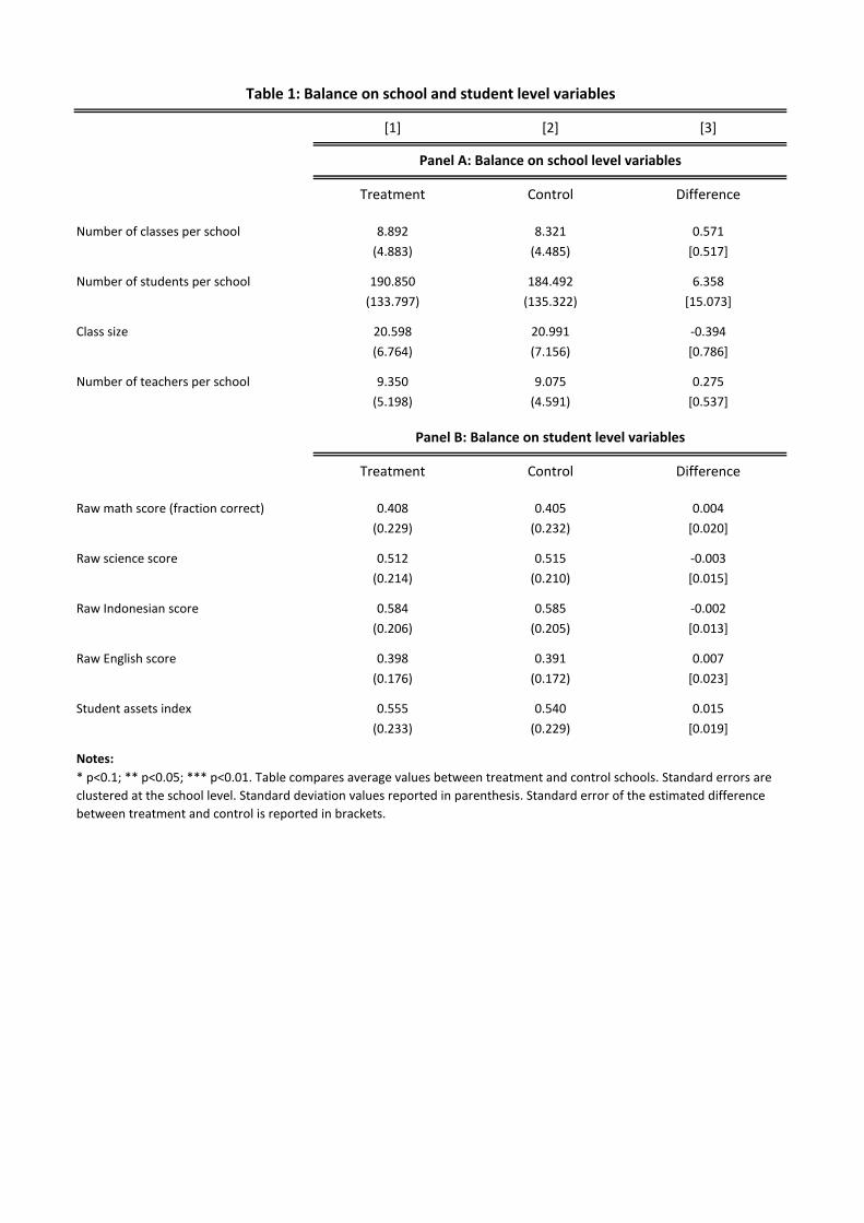
[1] [2] [3]

Treatment Control Difference

Number of classes per school 8.892 8.321 0.571

(4.883) (4.485) [0.517]

Number of students per school 190.850 184.492 6.358

(133.797) (135.322) [15.073]

Class size 20.598 20.991 -0.394

(6.764) (7.156) [0.786]

Number of teachers per school 9.350 9.075 0.275

(5.198) (4.591) [0.537]

Treatment Control Difference

Raw math score (fraction correct) 0.408 0.405 0.004

(0.229) (0.232) [0.020]

Raw science score 0.512 0.515 -0.003

(0.214) (0.210) [0.015]

Raw Indonesian score 0.584 0.585 -0.002

(0.206) (0.205) [0.013]

Raw English score 0.398 0.391 0.007

(0.176) (0.172) [0.023]

Student assets index 0.555 0.540 0.015

(0.233) (0.229) [0.019]

Notes:

* p<0.1; ** p<0.05; *** p<0.01. Table compares average values between treatment and control schools. Standard errors are

clustered at the school level. Standard deviation values reported in parenthesis. Standard error of the estimated difference

between treatment and control is reported in brackets.

Panel B: Balance on student level variables

Table 1: Balance on school and student level variables

Panel A: Balance on school level variables

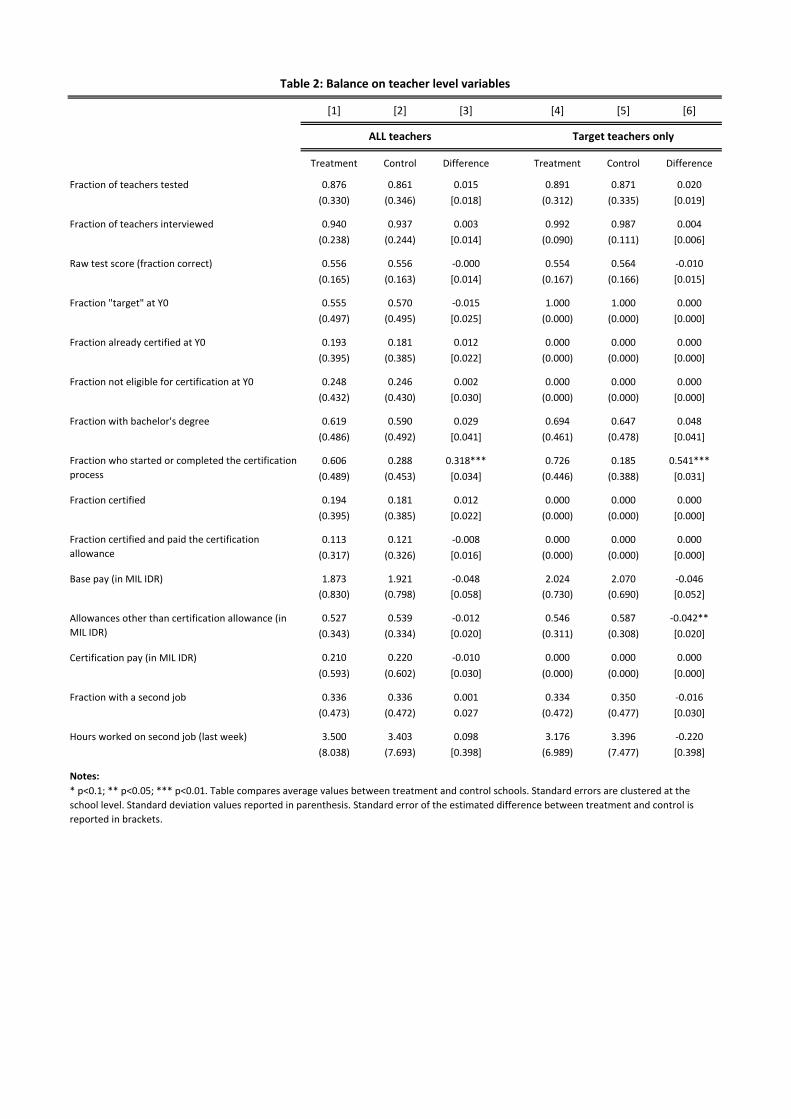
[1] [2] [3] [4] [5] [6]

Treatment Control Difference Treatment Control Difference

Fraction of teachers tested 0.876 0.861 0.015 0.891 0.871 0.020

(0.330) (0.346) [0.018] (0.312) (0.335) [0.019]

Fraction of teachers interviewed 0.940 0.937 0.003 0.992 0.987 0.004

(0.238) (0.244) [0.014] (0.090) (0.111) [0.006]

Raw test score (fraction correct) 0.556 0.556 -0.000 0.554 0.564 -0.010

(0.165) (0.163) [0.014] (0.167) (0.166) [0.015]

Fraction "target" at Y0 0.555 0.570 -0.015 1.000 1.000 0.000

(0.497) (0.495) [0.025] (0.000) (0.000) [0.000]

Fraction already certified at Y0 0.193 0.181 0.012 0.000 0.000 0.000

(0.395) (0.385) [0.022] (0.000) (0.000) [0.000]

Fraction not eligible for certification at Y0 0.248 0.246 0.002 0.000 0.000 0.000

(0.432) (0.430) [0.030] (0.000) (0.000) [0.000]

Fraction with bachelor's degree 0.619 0.590 0.029 0.694 0.647 0.048

(0.486) (0.492) [0.041] (0.461) (0.478) [0.041]

0.606 0.288 0.318*** 0.726 0.185 0.541***

(0.489) (0.453) [0.034] (0.446) (0.388) [0.031]

Fraction certified 0.194 0.181 0.012 0.000 0.000 0.000

(0.395) (0.385) [0.022] (0.000) (0.000) [0.000]

0.113 0.121 -0.008 0.000 0.000 0.000

(0.317) (0.326) [0.016] (0.000) (0.000) [0.000]

Base pay (in MIL IDR) 1.873 1.921 -0.048 2.024 2.070 -0.046

(0.830) (0.798) [0.058] (0.730) (0.690) [0.052]

0.527 0.539 -0.012 0.546 0.587 -0.042**

(0.343) (0.334) [0.020] (0.311) (0.308) [0.020]

Certification pay (in MIL IDR) 0.210 0.220 -0.010 0.000 0.000 0.000

(0.593) (0.602) [0.030] (0.000) (0.000) [0.000]

Fraction with a second job 0.336 0.336 0.001 0.334 0.350 -0.016

(0.473) (0.472) 0.027 (0.472) (0.477) [0.030]

Hours worked on second job (last week) 3.500 3.403 0.098 3.176 3.396 -0.220

(8.038) (7.693) [0.398] (6.989) (7.477) [0.398]

Notes:

* p<0.1; ** p<0.05; *** p<0.01. Table compares average values between treatment and control schools. Standard errors are clustered at the

school level. Standard deviation values reported in parenthesis. Standard error of the estimated difference between treatment and control is

reported in brackets.

ALL teachers Target teachers only

Table 2: Balance on teacher level variables

Fraction who started or completed the certification

process

Fraction certified and paid the certification

allowance

Allowances other than certification allowance (in

MIL IDR)

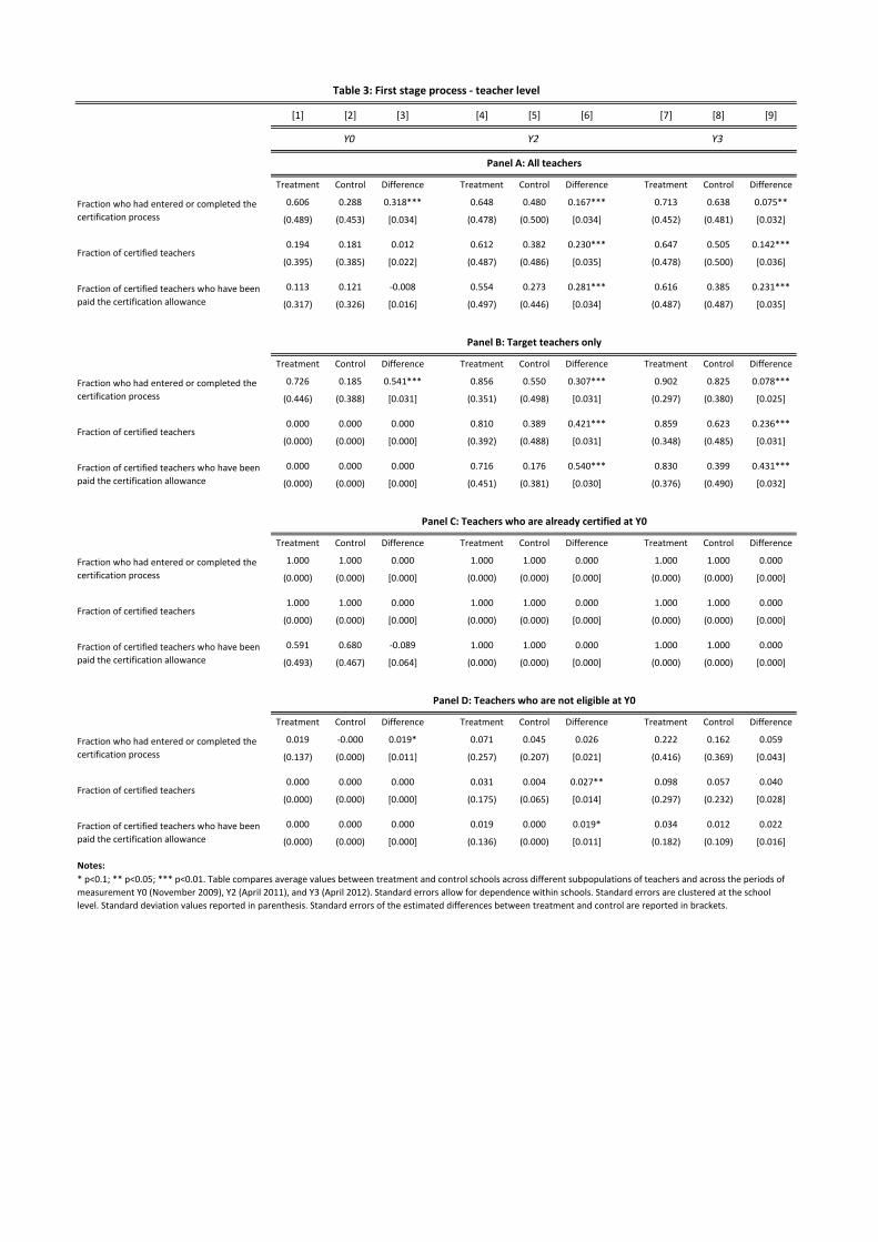
[1] [2] [3] [4] [5] [6] [7] [8] [9]

Treatment Control Difference Treatment Control Difference Treatment Control Difference

0.606 0.288 0.318*** 0.648 0.480 0.167*** 0.713 0.638 0.075**

(0.489) (0.453) [0.034] (0.478) (0.500) [0.034] (0.452) (0.481) [0.032]

0.194 0.181 0.012 0.612 0.382 0.230*** 0.647 0.505 0.142***

(0.395) (0.385) [0.022] (0.487) (0.486) [0.035] (0.478) (0.500) [0.036]

0.113 0.121 -0.008 0.554 0.273 0.281*** 0.616 0.385 0.231***

(0.317) (0.326) [0.016] (0.497) (0.446) [0.034] (0.487) (0.487) [0.035]

Treatment Control Difference Treatment Control Difference Treatment Control Difference

0.726 0.185 0.541*** 0.856 0.550 0.307*** 0.902 0.825 0.078***

(0.446) (0.388) [0.031] (0.351) (0.498) [0.031] (0.297) (0.380) [0.025]

0.000 0.000 0.000 0.810 0.389 0.421*** 0.859 0.623 0.236***

(0.000) (0.000) [0.000] (0.392) (0.488) [0.031] (0.348) (0.485) [0.031]

0.000 0.000 0.000 0.716 0.176 0.540*** 0.830 0.399 0.431***

(0.000) (0.000) [0.000] (0.451) (0.381) [0.030] (0.376) (0.490) [0.032]

Treatment Control Difference Treatment Control Difference Treatment Control Difference

1.000 1.000 0.000 1.000 1.000 0.000 1.000 1.000 0.000

(0.000) (0.000) [0.000] (0.000) (0.000) [0.000] (0.000) (0.000) [0.000]

1.000 1.000 0.000 1.000 1.000 0.000 1.000 1.000 0.000

(0.000) (0.000) [0.000] (0.000) (0.000) [0.000] (0.000) (0.000) [0.000]

0.591 0.680 -0.089 1.000 1.000 0.000 1.000 1.000 0.000

(0.493) (0.467) [0.064] (0.000) (0.000) [0.000] (0.000) (0.000) [0.000]

Treatment Control Difference Treatment Control Difference Treatment Control Difference

0.019 -0.000 0.019* 0.071 0.045 0.026 0.222 0.162 0.059

(0.137) (0.000) [0.011] (0.257) (0.207) [0.021] (0.416) (0.369) [0.043]

0.000 0.000 0.000 0.031 0.004 0.027** 0.098 0.057 0.040

(0.000) (0.000) [0.000] (0.175) (0.065) [0.014] (0.297) (0.232) [0.028]

0.000 0.000 0.000 0.019 0.000 0.019* 0.034 0.012 0.022

(0.000) (0.000) [0.000] (0.136) (0.000) [0.011] (0.182) (0.109) [0.016]

Notes:

* p<0.1; ** p<0.05; *** p<0.01. Table compares average values between treatment and control schools across different subpopulations of teachers and across the periods of

measurement Y0 (November 2009), Y2 (April 2011), and Y3 (April 2012). Standard errors allow for dependence within schools. Standard errors are clustered at the school

level. Standard deviation values reported in parenthesis. Standard errors of the estimated differences between treatment and control are reported in brackets.

Y0 Y2 Y3

Table 3: First stage process - teacher level

Panel A: All teachers

Panel B: Target teachers only

Panel C: Teachers who are already certified at Y0

Panel D: Teachers who are not eligible at Y0

Fraction who had entered or completed the

certification process

Fraction of certified teachers who have been

paid the certification allowance

Fraction who had entered or completed the

certification process

Fraction of certified teachers who have been

paid the certification allowance

Fraction who had entered or completed the

certification process

Fraction of certified teachers who have been

paid the certification allowance

Fraction who had entered or completed the

certification process

Fraction of certified teachers who have been

paid the certification allowance

Fraction of certified teachers

Fraction of certified teachers

Fraction of certified teachers

Fraction of certified teachers

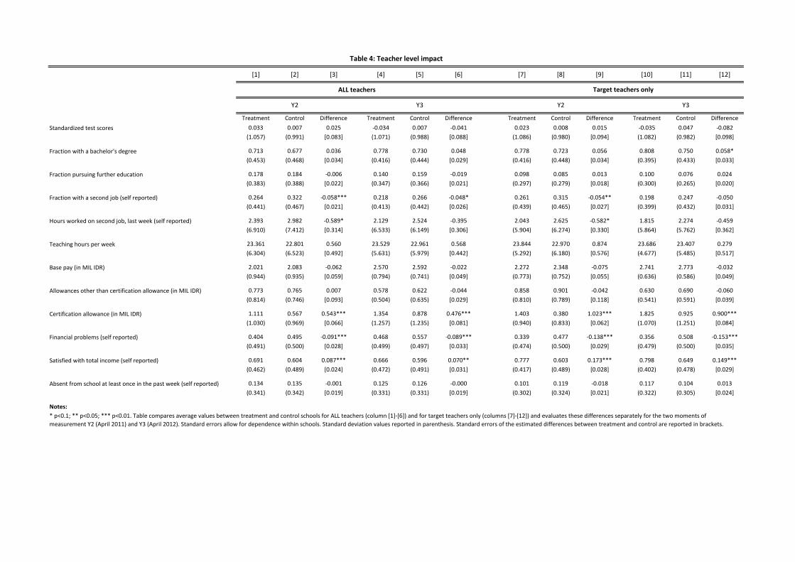
[1] [2] [3] [4] [5] [6] [7] [8] [9] [10] [11] [12]

Treatment Control Difference Treatment Control Difference Treatment Control Difference Treatment Control Difference

Standardized test scores 0.033 0.007 0.025 -0.034 0.007 -0.041 0.023 0.008 0.015 -0.035 0.047 -0.082

(1.057) (0.991) [0.083] (1.071) (0.988) [0.088] (1.086) (0.980) [0.094] (1.082) (0.982) [0.098]

Fraction with a bachelor's degree 0.713 0.677 0.036 0.778 0.730 0.048 0.778 0.723 0.056 0.808 0.750 0.058*

(0.453) (0.468) [0.034] (0.416) (0.444) [0.029] (0.416) (0.448) [0.034] (0.395) (0.433) [0.033]

Fraction pursuing further education 0.178 0.184 -0.006 0.140 0.159 -0.019 0.098 0.085 0.013 0.100 0.076 0.024

(0.383) (0.388) [0.022] (0.347) (0.366) [0.021] (0.297) (0.279) [0.018] (0.300) (0.265) [0.020]

Fraction with a second job (self reported) 0.264 0.322 -0.058*** 0.218 0.266 -0.048* 0.261 0.315 -0.054** 0.198 0.247 -0.050

(0.441) (0.467) [0.021] (0.413) (0.442) [0.026] (0.439) (0.465) [0.027] (0.399) (0.432) [0.031]

Hours worked on second job, last week (self reported) 2.393 2.982 -0.589* 2.129 2.524 -0.395 2.043 2.625 -0.582* 1.815 2.274 -0.459

(6.910) (7.412) [0.314] (6.533) (6.149) [0.306] (5.904) (6.274) [0.330] (5.864) (5.762) [0.362]

Teaching hours per week 23.361 22.801 0.560 23.529 22.961 0.568 23.844 22.970 0.874 23.686 23.407 0.279

(6.304) (6.523) [0.492] (5.631) (5.979) [0.442] (5.292) (6.180) [0.576] (4.677) (5.485) [0.517]

Base pay (in MIL IDR) 2.021 2.083 -0.062 2.570 2.592 -0.022 2.272 2.348 -0.075 2.741 2.773 -0.032

(0.944) (0.935) [0.059] (0.794) (0.741) [0.049] (0.773) (0.752) [0.055] (0.636) (0.586) [0.049]

Allowances other than certification allowance (in MIL IDR) 0.773 0.765 0.007 0.578 0.622 -0.044 0.858 0.901 -0.042 0.630 0.690 -0.060

(0.814) (0.746) [0.093] (0.504) (0.635) [0.029] (0.810) (0.789) [0.118] (0.541) (0.591) [0.039]

Certification allowance (in MIL IDR) 1.111 0.567 0.543*** 1.354 0.878 0.476*** 1.403 0.380 1.023*** 1.825 0.925 0.900***

(1.030) (0.969) [0.066] (1.257) (1.235) [0.081] (0.940) (0.833) [0.062] (1.070) (1.251) [0.084]

Financial problems (self reported) 0.404 0.495 -0.091*** 0.468 0.557 -0.089*** 0.339 0.477 -0.138*** 0.356 0.508 -0.153***

(0.491) (0.500) [0.028] (0.499) (0.497) [0.033] (0.474) (0.500) [0.029] (0.479) (0.500) [0.035]

Satisfied with total income (self reported) 0.691 0.604 0.087*** 0.666 0.596 0.070** 0.777 0.603 0.173*** 0.798 0.649 0.149***

(0.462) (0.489) [0.024] (0.472) (0.491) [0.031] (0.417) (0.489) [0.028] (0.402) (0.478) [0.029]

Absent from school at least once in the past week (self reported) 0.134 0.135 -0.001 0.125 0.126 -0.000 0.101 0.119 -0.018 0.117 0.104 0.013

(0.341) (0.342) [0.019] (0.331) (0.331) [0.019] (0.302) (0.324) [0.021] (0.322) (0.305) [0.024]

Notes:

Table 4: Teacher level impact

ALL teachers Target teachers only

* p<0.1; ** p<0.05; *** p<0.01. Table compares average values between treatment and control schools for ALL teachers (column [1]-[6]) and for target teachers only (columns [7]-[12]) and evaluates these differences separately for the two moments of

measurement Y2 (April 2011) and Y3 (April 2012). Standard errors allow for dependence within schools. Standard deviation values reported in parenthesis. Standard errors of the estimated differences between treatment and control are reported in brackets.

Y2 Y3 Y2 Y3

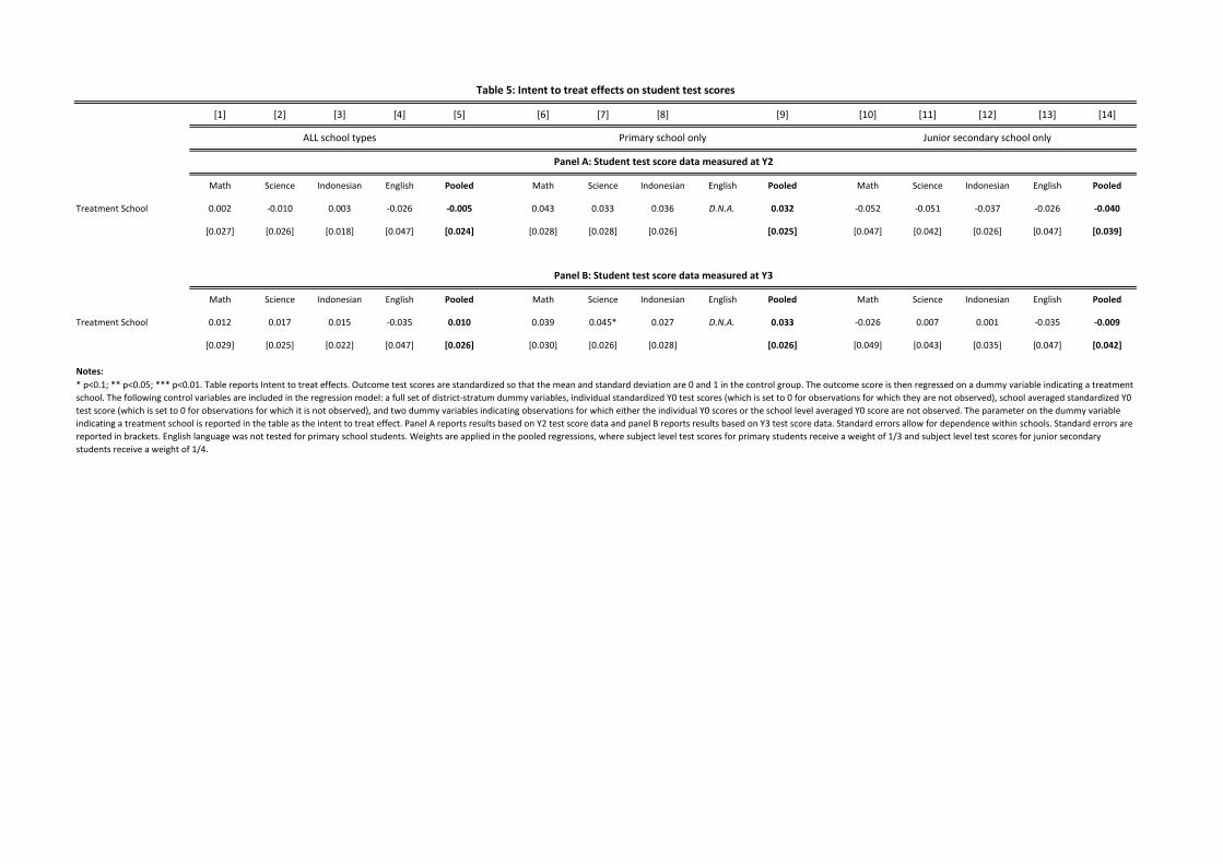
[1] [2] [3] [4] [5] [6] [7] [8] [9] [10] [11] [12] [13] [14]

Math Science Indonesian English Pooled Math Science Indonesian English Pooled Math Science Indonesian English Pooled

Treatment School 0.002 -0.010 0.003 -0.026 -0.005 0.043 0.033 0.036 D.N.A. 0.032 -0.052 -0.051 -0.037 -0.026 -0.040

[0.027] [0.026] [0.018] [0.047] [0.024] [0.028] [0.028] [0.026] [0.025] [0.047] [0.042] [0.026] [0.047] [0.039]

Math Science Indonesian English Pooled Math Science Indonesian English Pooled Math Science Indonesian English Pooled

Treatment School 0.012 0.017 0.015 -0.035 0.010 0.039 0.045* 0.027 D.N.A. 0.033 -0.026 0.007 0.001 -0.035 -0.009

[0.029] [0.025] [0.022] [0.047] [0.026] [0.030] [0.026] [0.028] [0.026] [0.049] [0.043] [0.035] [0.047] [0.042]

Notes:

Table 5: Intent to treat effects on student test scores

Panel A: Student test score data measured at Y2

Panel B: Student test score data measured at Y3

* p<0.1; ** p<0.05; *** p<0.01. Table reports Intent to treat effects. Outcome test scores are standardized so that the mean and standard deviation are 0 and 1 in the control group. The outcome score is then regressed on a dummy variable indicating a treatment

school. The following control variables are included in the regression model: a full set of district-stratum dummy variables, individual standardized Y0 test scores (which is set to 0 for observations for which they are not observed), school averaged standardized Y0

test score (which is set to 0 for observations for which it is not observed), and two dummy variables indicating observations for which either the individual Y0 scores or the school level averaged Y0 score are not observed. The parameter on the dummy variable

indicating a treatment school is reported in the table as the intent to treat effect. Panel A reports results based on Y2 test score data and panel B reports results based on Y3 test score data. Standard errors allow for dependence within schools. Standard errors are

reported in brackets. English language was not tested for primary school students. Weights are applied in the pooled regressions, where subject level test scores for primary students receive a weight of 1/3 and subject level test scores for junior secondary

students receive a weight of 1/4.

ALL school types Primary school only Junior secondary school only

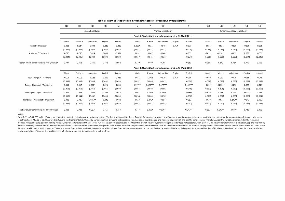
[1] [2] [3] [4] [5] [6] [7] [8] [9] [10] [11] [12] [13] [14]

Math Science Indonesian English Pooled Math Science Indonesian English Pooled Math Science Indonesian English Pooled

Target * Treatment 0.011 -0.014 0.003 -0.030 -0.006 0.065* 0.021 0.040 D.N.A. 0.031 -0.053 -0.021 -0.029 -0.030 -0.035

[0.034] [0.032] [0.022] [0.044] [0.026] [0.037] [0.033] [0.032] [0.029] [0.056] [0.054] [0.032] [0.044] [0.038]

Nontarget * Treatment -0.015 -0.015 0.014 0.009 -0.001 0.032 0.047 0.044 0.039 -0.092 -0.118** -0.039 0.009 -0.051

[0.034] [0.036] [0.029] [0.074] [0.030] [0.037] [0.041] [0.037] [0.034] [0.058] [0.060] [0.038] [0.074] [0.048]

test all causal parameters are zero (p-value) 0.797 0.858 0.886 0.772 0.962 0.170 0.440 0.268 0.363 0.260 0.142 0.434 0.772 0.555

Math Science Indonesian English Pooled Math Science Indonesian English Pooled Math Science Indonesian English Pooled

Target - Target * Treatment -0.020 -0.003 -0.035 -0.059 -0.025 0.031 -0.012 0.019 D.N.A. 0.006 -0.089 0.061 -0.079 -0.059 -0.045

[0.047] [0.046] [0.036] [0.052] [0.033] [0.052] [0.046] [0.045] [0.038] [0.078] [0.082] [0.055] [0.052] [0.048]

Target - Nontarget * Treatment 0.055 0.017 0.087* 0.026 0.054 0.117** 0.128*** 0.177*** 0.132*** -0.069 -0.233** -0.072 0.026 -0.061

[0.058] [0.051] [0.051] [0.066] [0.040] [0.054] [0.049] [0.058] [0.046] [0.117] [0.108] [0.087] [0.066] [0.062]

Nontarget - Target * Treatment 0.016 0.033 0.005 -0.023 0.018 0.042 -0.004 -0.035 -0.006 -0.016 0.109* 0.042 -0.023 0.038

[0.052] [0.044] [0.042] [0.056] [0.039] [0.058] [0.060] [0.050] [0.050] [0.077] [0.057] [0.068] [0.056] [0.054]

Nontarget - Nontarget * Treatment 0.008 0.025 0.086** -0.042 0.032 0.027 0.075* 0.054 0.053 -0.029 -0.071 0.146** -0.042 0.005

[0.051] [0.040] [0.040] [0.071] [0.036] [0.048] [0.043] [0.045] [0.041] [0.111] [0.061] [0.071] [0.071] [0.059]

Test all causal parameters are zero (p-value) 0.811 0.922 0.097* 0.715 0.353 0.247 0.059* 0.016** 0.047** 0.817 0.042** 0.089* 0.715 0.452

Notes:

* p<0.1; ** p<0.05; *** p<0.01. Table reports intent to treat effects, broken down by type of teacher. The first row in panel B -- Target-Target -- for example measures the difference in learning outcomes between treatment and control for the subpopulation of students who had a

target teacher in Y2 AND in Y3. These are the students most (differentially) affected by our intervention. Outcome test scores are standardized so that the mean and standard deviation is 0 and 1 in the control group. The following control variables are included in the regression

model: a full set of district-stratum dummy variables, individual standardized Y0 test scores (which is set to 0 for observations for which they are not observed), school averaged standardized Y0 test score (which is set to 0 for observations for which it is not observed), and two dummy

variables indicating observations for which either the individual Y0 scores or the school level averaged Y0 score are not observed. The parameters reported in the table are the intent to treat effect for different subpopulations of students. Panel A reports results based on Y2 test score

data and panel B reports results based on Y3 test score data. Standard errors allow for dependence within schools. Standard errors are reported in brackets. Weights are applied in the pooled regressions presented in column [4], where subject level test scores for primary students

receive a weight of 1/3 and subject level test scores for junior secondary students receive a weight of 1/4.

Table 6: Intent to treat effects on student test scores -- breakdown by target status

ALL school types Primary school only Junior secondary school only

Panel A: Student test score data measured at Y2 (April 2011)

Panel B: Student test score data measured at Y3 (April 2012)

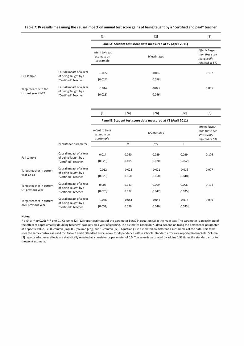
[1] [2] [3]

Intent to treat

estimate on

subsample

IV estimates

Effects larger

than these are

statistically

rejected at 5%

-0.005 -0.016 0.137

[0.024] [0.078]

-0.014 -0.025 0.065

[0.025] [0.046]

[1] [2a] [2b] [2c] [3]

Intent to treat

estimate on

subsample

IV estimates

Effects larger

than these are

statistically

rejected at 5%

Persistence parameter 0 0.5 1

0.014 0.060 0.039 0.029 0.176

[0.026] [0.105] [0.070] [0.052]

-0.012 -0.028 -0.021 -0.016 0.077

[0.029] [0.068] [0.050] [0.040]

0.005 0.013 0.009 0.006 0.101

[0.026] [0.072] [0.047] [0.035]

-0.036 -0.084 -0.051 -0.037 0.039

[0.032] [0.076] [0.046] [0.033]

Notes:

Table 7: IV results measuring the causal impact on annual test score gains of being taught by a "certified and paid" teacher

* p<0.1; ** p<0.05; *** p<0.01. Columns [2]-[12] report estimates of the parameter beta2 in equation (3) in the main text. The parameter is an estimate of

the effect of approximately doubling teachers' base pay on a year of learning. The estimates based on Y3 data depend on fixing the persistence parameter

at a specific value, i.e. 0 (column [2a]), 0.5 (column [2b]), and 1 (column [2c]). Equation (3) is estimated on different a subsamples of the data. This table

uses the same controls as used for Table 5 and 6. Standard errors allow for dependence within schools. Standard errors are reported in brackets. Column

[3] reports whichever effects are statistically rejected at a persistence parameter of 0.5. The value is calculated by adding 1.96 times the standard error to

the point estimate.

Target teacher in current

OR previous year

Causal Impact of a Year

of being Taught by a

"Certified" Teacher

Target teacher in current

AND previous year

Causal Impact of a Year

of being Taught by a

"Certified" Teacher

Panel B: Student test score data measured at Y3 (April 2011)

Target teacher in current

year Y2-Y3

Causal Impact of a Year

of being Taught by a

"Certified" Teacher

Full sample

Target teacher in the

current year Y1-Y2

Causal Impact of a Year

of being Taught by a

"Certified" Teacher

Full sample

Causal Impact of a Year

of being Taught by a

"Certified" Teacher

Causal Impact of a Year

of being Taught by a

"Certified" Teacher

Panel A: Student test score data measured at Y2 (April 2011)

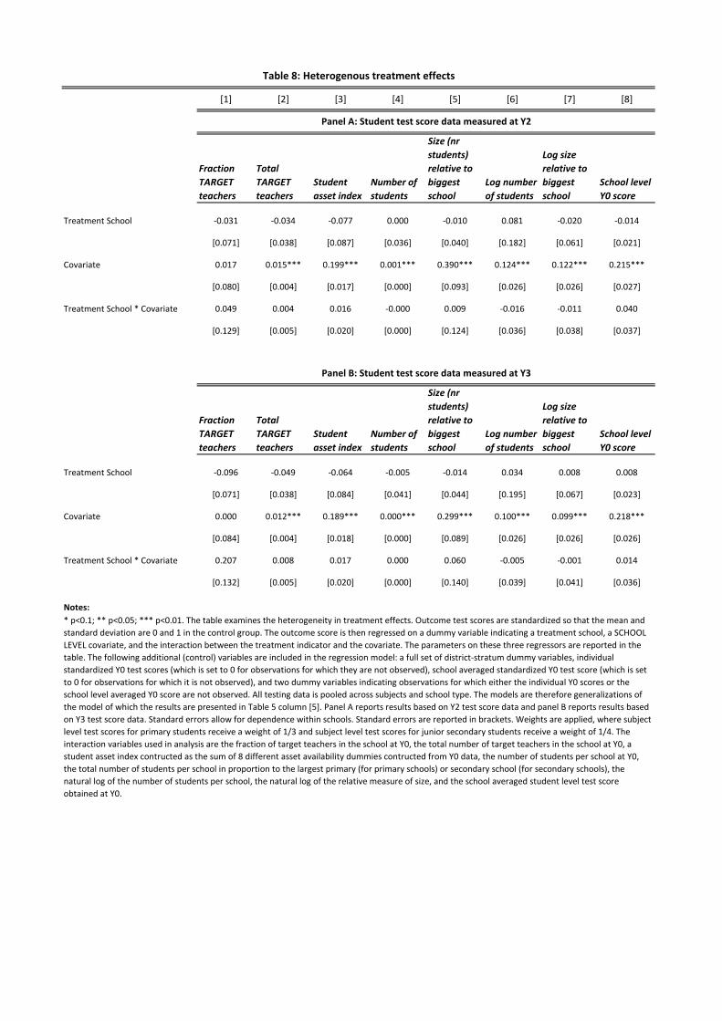
[1] [2] [3] [4] [5] [6] [7] [8]

Fraction

TARGET

teachers

Total

TARGET

teachers

Student

asset index

Number of

students

Size (nr

students)

relative to

biggest

school

Log number

of students

Log size

relative to

biggest

school

School level

Y0 score

Treatment School -0.031 -0.034 -0.077 0.000 -0.010 0.081 -0.020 -0.014

[0.071] [0.038] [0.087] [0.036] [0.040] [0.182] [0.061] [0.021]

Covariate 0.017 0.015*** 0.199*** 0.001*** 0.390*** 0.124*** 0.122*** 0.215***

[0.080] [0.004] [0.017] [0.000] [0.093] [0.026] [0.026] [0.027]

Treatment School * Covariate 0.049 0.004 0.016 -0.000 0.009 -0.016 -0.011 0.040

[0.129] [0.005] [0.020] [0.000] [0.124] [0.036] [0.038] [0.037]

Fraction

TARGET

teachers

Total

TARGET

teachers

Student

asset index

Number of

students

Size (nr

students)

relative to

biggest

school

Log number

of students

Log size

relative to

biggest

school

School level

Y0 score

Treatment School -0.096 -0.049 -0.064 -0.005 -0.014 0.034 0.008 0.008

[0.071] [0.038] [0.084] [0.041] [0.044] [0.195] [0.067] [0.023]

Covariate 0.000 0.012*** 0.189*** 0.000*** 0.299*** 0.100*** 0.099*** 0.218***

[0.084] [0.004] [0.018] [0.000] [0.089] [0.026] [0.026] [0.026]

Treatment School * Covariate 0.207 0.008 0.017 0.000 0.060 -0.005 -0.001 0.014

[0.132] [0.005] [0.020] [0.000] [0.140] [0.039] [0.041] [0.036]

Notes:

* p<0.1; ** p<0.05; *** p<0.01. The table examines the heterogeneity in treatment effects. Outcome test scores are standardized so that the mean and

standard deviation are 0 and 1 in the control group. The outcome score is then regressed on a dummy variable indicating a treatment school, a SCHOOL

LEVEL covariate, and the interaction between the treatment indicator and the covariate. The parameters on these three regressors are reported in the

table. The following additional (control) variables are included in the regression model: a full set of district-stratum dummy variables, individual

standardized Y0 test scores (which is set to 0 for observations for which they are not observed), school averaged standardized Y0 test score (which is set

to 0 for observations for which it is not observed), and two dummy variables indicating observations for which either the individual Y0 scores or the

school level averaged Y0 score are not observed. All testing data is pooled across subjects and school type. The models are therefore generalizations of

the model of which the results are presented in Table 5 column [5]. Panel A reports results based on Y2 test score data and panel B reports results based

on Y3 test score data. Standard errors allow for dependence within schools. Standard errors are reported in brackets. Weights are applied, where subject

level test scores for primary students receive a weight of 1/3 and subject level test scores for junior secondary students receive a weight of 1/4. The

interaction variables used in analysis are the fraction of target teachers in the school at Y0, the total number of target teachers in the school at Y0, a

student asset index contructed as the sum of 8 different asset availability dummies contructed from Y0 data, the number of students per school at Y0,

the total number of students per school in proportion to the largest primary (for primary schools) or secondary school (for secondary schools), the

natural log of the number of students per school, the natural log of the relative measure of size, and the school averaged student level test score

obtained at Y0.

Table 8: Heterogenous treatment effects

Panel A: Student test score data measured at Y2

Panel B: Student test score data measured at Y3

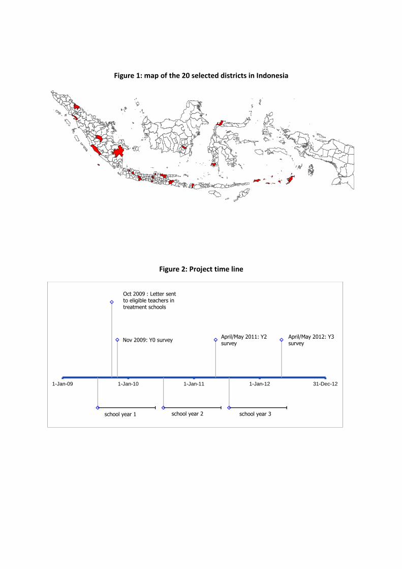
Figure 1: map of the 20 selected districts in Indonesia

Figure 2: Project time line

Nov 2009: Y0 surveyApril/May 2011: Y2 survey

April/May 2012: Y3 survey

Oct 2009 : Letter sent to eligible teachers in treatment schools

school year 1 school year 2 school year 3

1-Jan-09 1-Jan-10 1-Jan-11 1-Jan-12 31-Dec-12

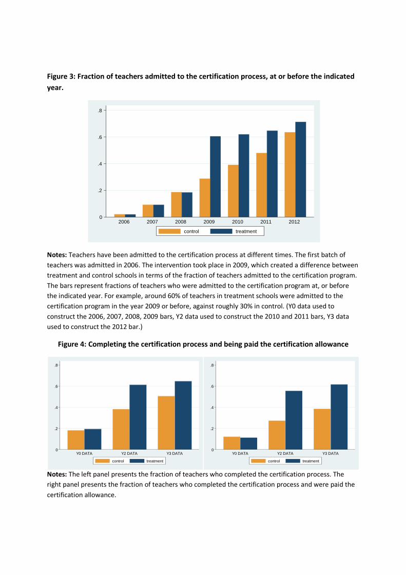
Figure 3: Fraction of teachers admitted to the certification process, at or before the indicated

year.

Notes: Teachers have been admitted to the certification process at different times. The first batch of

teachers was admitted in 2006. The intervention took place in 2009, which created a difference between

treatment and control schools in terms of the fraction of teachers admitted to the certification program.

The bars represent fractions of teachers who were admitted to the certification program at, or before

the indicated year. For example, around 60% of teachers in treatment schools were admitted to the

certification program in the year 2009 or before, against roughly 30% in control. (Y0 data used to

construct the 2006, 2007, 2008, 2009 bars, Y2 data used to construct the 2010 and 2011 bars, Y3 data

used to construct the 2012 bar.)

Figure 4: Completing the certification process and being paid the certification allowance

Notes: The left panel presents the fraction of teachers who completed the certification process. The

right panel presents the fraction of teachers who completed the certification process and were paid the

certification allowance.

0

.2

.4

.6

.8

2006 2007 2008 2009 2010 2011 2012

control treatment

0

.2

.4

.6

.8

Y0 DATA Y2 DATA Y3 DATA

control treatment

0

.2

.4

.6

.8

Y0 DATA Y2 DATA Y3 DATA

control treatment

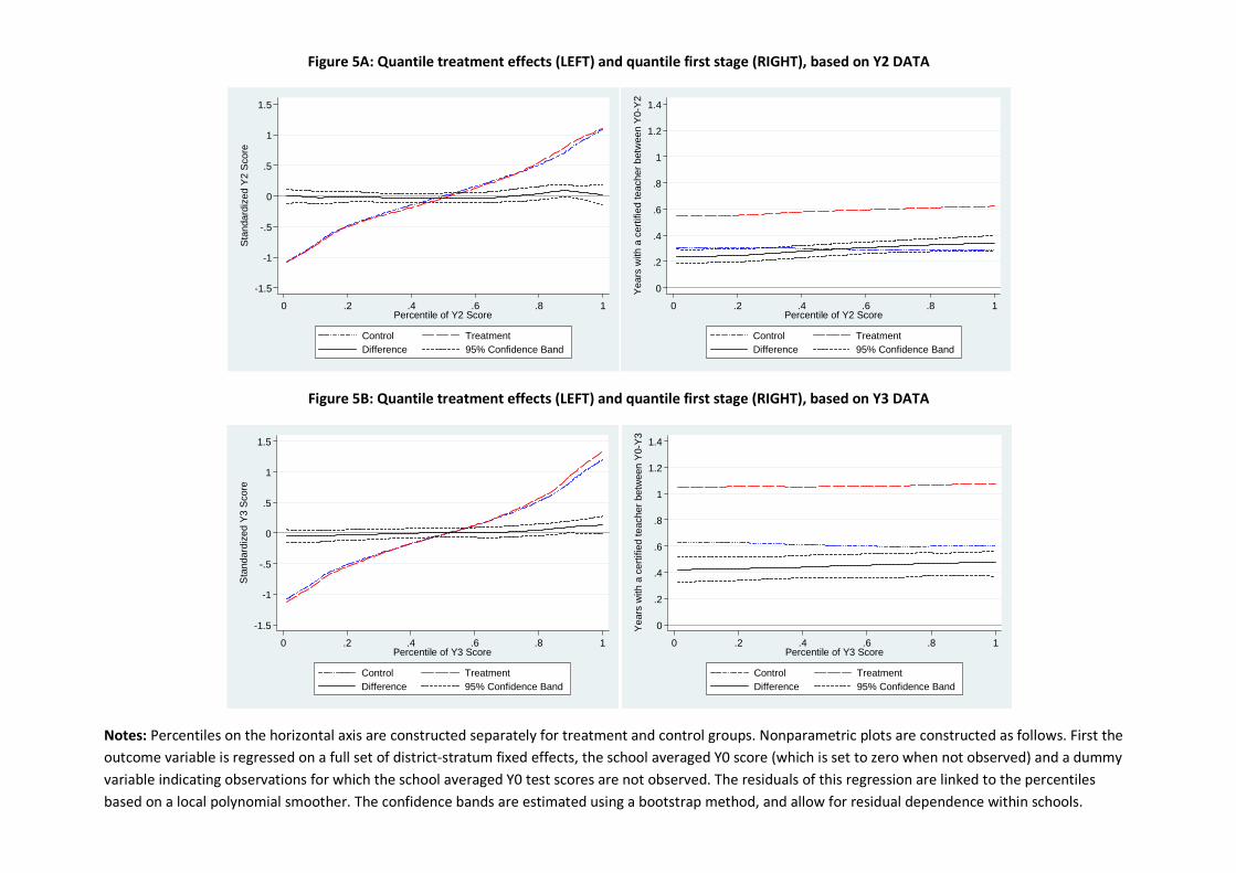
Figure 5A: Quantile treatment effects (LEFT) and quantile first stage (RIGHT), based on Y2 DATA

Figure 5B: Quantile treatment effects (LEFT) and quantile first stage (RIGHT), based on Y3 DATA

Notes: Percentiles on the horizontal axis are constructed separately for treatment and control groups. Nonparametric plots are constructed as follows. First the

outcome variable is regressed on a full set of district-stratum fixed effects, the school averaged Y0 score (which is set to zero when not observed) and a dummy

variable indicating observations for which the school averaged Y0 test scores are not observed. The residuals of this regression are linked to the percentiles

based on a local polynomial smoother. The confidence bands are estimated using a bootstrap method, and allow for residual dependence within schools.

-1.5

-1

-.5

0

.5

1

1.5

Sta

ndar

dize

d Y

2 S

core

0 .2 .4 .6 .8 1Percentile of Y2 Score

Control TreatmentDifference 95% Confidence Band

0

.2

.4

.6

.8

1

1.2

1.4

Yea

rs w

ith a

cer

tifie

d te

ache

r be

twee

n Y

0-Y

2

0 .2 .4 .6 .8 1Percentile of Y2 Score

Control TreatmentDifference 95% Confidence Band

-1.5

-1

-.5

0

.5

1

1.5

Sta

ndar

dize

d Y

3 S

core

0 .2 .4 .6 .8 1Percentile of Y3 Score

Control TreatmentDifference 95% Confidence Band

0

.2

.4

.6

.8

1

1.2

1.4

Yea

rs w

ith a

cer

tifie

d te

ache

r be

twee

n Y

0-Y

30 .2 .4 .6 .8 1

Percentile of Y3 Score

Control TreatmentDifference 95% Confidence Band

Strata Sampled districts

Eastern Indonesia (Maluku and Papua) Maluku Tenggara Barat

Nusa Tenggara Lombok Timur

Western Java Ciamis, Jakarta Timur, Purwakarta

Central Java Bantul, Kudus, Semarang

Eastern Java + Bali Lamongan, Lumajang, Probolinggo, Tuban

Kalimantan Hulu Sungai Selatan

Sulawesi Gowa, Toli Toli

Northern Sumatra Deli Serdang, Tapanuli Tengah

Western Sumatra Tebo

Southern Sumatra Bengkulu Utara, Ogan Ilir

Notes:

Table A.1: Strata and sampled districts

Regions (the strata) are approximate descriptions. Western Java, for example, includes the provinces West Java, Jakarta and Banten, all three located on the western

side of the island of Java

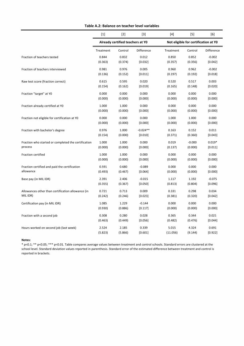
[1] [2] [3] [4] [5] [6]

Treatment Control Difference Treatment Control Difference

Fraction of teachers tested 0.844 0.832 0.012 0.850 0.852 -0.002

(0.363) (0.374) [0.032] (0.357) (0.356) [0.042]

Fraction of teachers interviewed 0.981 0.976 0.005 0.960 0.962 -0.002

(0.136) (0.152) [0.011] (0.197) (0.192) [0.018]

Raw test score (fraction correct) 0.615 0.595 0.020 0.520 0.517 0.003

(0.154) (0.162) [0.019] (0.165) (0.148) [0.020]

Fraction "target" at Y0 0.000 0.000 0.000 0.000 0.000 0.000

(0.000) (0.000) [0.000] (0.000) (0.000) [0.000]

Fraction already certified at Y0 1.000 1.000 0.000 0.000 0.000 0.000

(0.000) (0.000) [0.000] (0.000) (0.000) [0.000]

Fraction not eligible for certification at Y0 0.000 0.000 0.000 1.000 1.000 0.000

(0.000) (0.000) [0.000] (0.000) (0.000) [0.000]

Fraction with bachelor's degree 0.976 1.000 -0.024** 0.163 0.152 0.011

(0.154) (0.000) [0.010] (0.371) (0.360) [0.043]

1.000 1.000 0.000 0.019 -0.000 0.019*

(0.000) (0.000) [0.000] (0.137) (0.000) [0.011]

Fraction certified 1.000 1.000 0.000 0.000 0.000 0.000

(0.000) (0.000) [0.000] (0.000) (0.000) [0.000]

0.591 0.680 -0.089 0.000 0.000 0.000

(0.493) (0.467) [0.064] (0.000) (0.000) [0.000]

Base pay (in MIL IDR) 2.391 2.406 -0.015 1.117 1.192 -0.075

(0.355) (0.367) [0.050] (0.813) (0.804) [0.096]

0.721 0.713 0.009 0.331 0.298 0.034

(0.242) (0.246) [0.023] (0.381) (0.320) [0.042]

Certification pay (in MIL IDR) 1.085 1.229 -0.144 0.000 0.000 0.000

(0.930) (0.886) [0.117] (0.000) (0.000) [0.000]

Fraction with a second job 0.308 0.280 0.028 0.365 0.344 0.021

(0.463) (0.449) [0.056] (0.482) (0.476) [0.044]

Hours worked on second job (last week) 2.524 2.185 0.339 5.015 4.324 0.691

(5.823) (5.866) [0.601] (11.056) (9.144) [0.922]

Notes:

* p<0.1; ** p<0.05; *** p<0.01. Table compares average values between treatment and control schools. Standard errors are clustered at the

school level. Standard deviation values reported in parenthesis. Standard error of the estimated difference between treatment and control is

reported in brackets.

Table A.2: Balance on teacher level variables

Already certified teachers at Y0 Not eligible for certification at Y0

Fraction who started or completed the certification

process

Fraction certified and paid the certification

allowance

Allowances other than certification allowance (in

MIL IDR)

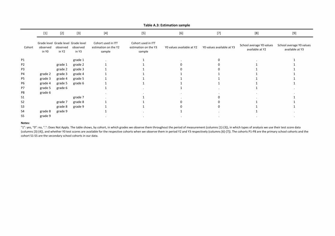
[1] [2] [3] [4] [5] [6] [7] [8] [9]

Cohort

Grade level

observed

in Y0

Grade level

observed

in Y2

Grade level

observed

in Y3

Cohort used in ITT

estimation on the Y2

sample

Cohort used in ITT

estimation on the Y3

sample

Y0 values available at Y2 Y0 values available at Y3School average Y0 values

available at Y2

School average Y0 values

available at Y3

P1 grade 1 . 1 . 0 . 1

P2 grade 1 grade 2 1 1 0 0 1 1

P3 grade 2 grade 3 1 1 0 0 1 1

P4 grade 2 grade 3 grade 4 1 1 1 1 1 1

P5 grade 3 grade 4 grade 5 1 1 1 1 1 1

P6 grade 4 grade 5 grade 6 1 1 1 1 1 1

P7 grade 5 grade 6 1 . 1 . 1 .

P8 grade 6 . . . . . .

S1 grade 7 . 1 . 0 . 1

S2 grade 7 grade 8 1 1 0 0 1 1

S3 grade 8 grade 9 1 1 0 0 1 1

S4 grade 8 grade 9 1 . 1 . 1 .

S5 grade 9 . . . . . .

Notes:

Table A.3: Estimation sample

"1": yes, "0": no, ".": Does Not Apply. The table shows, by cohort, in which grades we observe them throughout the period of measurement (columns [1]-[3]), in which types of analysis we use their test score data

(columns [3]-[4]), and whether Y0 test scores are available for the respective cohorts when we observe them in period Y2 and Y3 respectively (columns [6]-[7]). The cohorts P1-P8 are the primary school cohorts and the

cohort S1-S5 are the secondary school cohorts in our data.

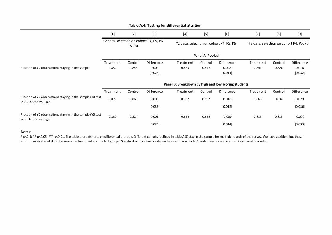
[1] [2] [3] [4] [5] [6] [7] [8] [9]

Treatment Control Difference Treatment Control Difference Treatment Control Difference

Fraction of Y0 observations staying in the sample 0.854 0.845 0.009 0.885 0.877 0.008 0.841 0.826 0.016

[0.024] [0.011] [0.032]

Treatment Control Difference Treatment Control Difference Treatment Control Difference

Fraction of Y0 observations staying in the sample (Y0 test

score above average)0.878 0.869 0.009 0.907 0.892 0.016 0.863 0.834 0.029

[0.033] [0.012] [0.036]

Fraction of Y0 observations staying in the sample (Y0 test

score below average)0.830 0.824 0.006 0.859 0.859 -0.000 0.815 0.815 -0.000

[0.020] [0.014] [0.033]

Notes:* p<0.1; ** p<0.05; *** p<0.01. The table presents tests on differential attrition. Different cohorts (defined in table A.3) stay in the sample for multiple rounds of the survey. We have attrition, but these

attrition rates do not differ between the treatment and control groups. Standard errors allow for dependence within schools. Standard errors are reported in squared brackets.

Table A.4: Testing for differential attrition

Y2 data, selection on cohort P4, P5, P6,

P7, S4Y2 data, selection on cohort P4, P5, P6 Y3 data, selection on cohort P4, P5, P6

Panel A: Pooled

Panel B: Breakdown by high and low scoring students

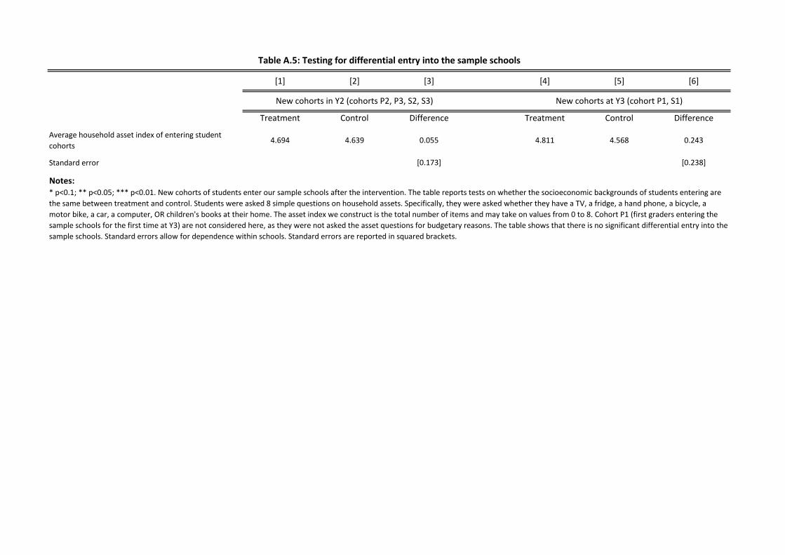
[1] [2] [3] [4] [5] [6]

Treatment Control Difference Treatment Control Difference

Average household asset index of entering student

cohorts4.694 4.639 0.055 4.811 4.568 0.243

Standard error [0.173] [0.238]

Notes:

Table A.5: Testing for differential entry into the sample schools

New cohorts in Y2 (cohorts P2, P3, S2, S3) New cohorts at Y3 (cohort P1, S1)

* p<0.1; ** p<0.05; *** p<0.01. New cohorts of students enter our sample schools after the intervention. The table reports tests on whether the socioeconomic backgrounds of students entering are

the same between treatment and control. Students were asked 8 simple questions on household assets. Specifically, they were asked whether they have a TV, a fridge, a hand phone, a bicycle, a

motor bike, a car, a computer, OR children's books at their home. The asset index we construct is the total number of items and may take on values from 0 to 8. Cohort P1 (first graders entering the

sample schools for the first time at Y3) are not considered here, as they were not asked the asset questions for budgetary reasons. The table shows that there is no significant differential entry into the

sample schools. Standard errors allow for dependence within schools. Standard errors are reported in squared brackets.

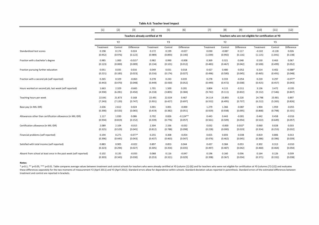
[1] [2] [3] [4] [5] [6] [7] [8] [9] [10] [11] [12]

Treatment Control Difference Treatment Control Difference Treatment Control Difference Treatment Control Difference

Standardized test scores 0.198 0.174 0.024 0.172 0.199 -0.027 0.030 -0.087 0.117 -0.102 -0.128 0.026

(0.952) (0.976) [0.122] (0.989) (0.893) [0.140] (1.039) (0.992) [0.116] (1.115) (1.041) [0.138]

Fraction with a bachelor's degree 0.985 1.000 -0.015* 0.982 0.990 -0.008 0.369 0.321 0.048 0.530 0.463 0.067

(0.123) (0.000) [0.009] (0.134) (0.101) [0.012] (0.483) (0.467) [0.042] (0.500) (0.499) [0.052]

Fraction pursuing further education 0.051 0.035 0.016 0.049 0.031 0.018 0.427 0.480 -0.052 0.314 0.402 -0.088*

(0.221) (0.183) [0.023] (0.216) (0.174) [0.027] (0.496) (0.500) [0.045] (0.465) (0.491) [0.048]

Fraction with a second job (self reported) 0.265 0.329 -0.063 0.278 0.243 0.035 0.278 0.333 -0.054 0.220 0.297 -0.077*

(0.443) (0.470) [0.048] (0.449) (0.430) [0.052] (0.449) (0.472) [0.038] (0.415) (0.457) [0.043]

Hours worked on second job, last week (self reported) 1.663 2.329 -0.665 1.701 1.500 0.201 3.804 4.115 -0.311 3.136 3.472 -0.335

(4.930) (6.281) [0.450] (4.218) (3.805) [0.384] (9.742) (9.111) [0.832] (9.152) (7.546) [0.847]

Teaching hours per week 22.041 21.873 0.168 22.491 22.024 0.467 24.114 23.893 0.220 24.798 23.901 0.897

(7.243) (7.120) [0.747] (5.931) (6.427) [0.697] (6.552) (6.495) [0.737] (6.212) (5.265) [0.826]

Base pay (in MIL IDR) 2.636 2.612 0.024 3.001 3.001 -0.000 1.279 1.366 -0.087 1.904 1.959 -0.055

(0.390) (0.533) [0.065] (0.419) (0.382) [0.051] (0.929) (0.938) [0.095] (0.868) (0.798) [0.101]

Allowances other than certification allowance (in MIL IDR) 1.117 1.030 0.086 0.702 0.826 -0.124** 0.443 0.443 -0.001 0.442 0.458 -0.016

(0.934) (0.819) [0.152] (0.339) (0.776) [0.057] (0.561) (0.509) [0.054] (0.522) (0.649) [0.057]

Certification allowance (in MIL IDR) 2.089 2.104 -0.015 2.304 2.336 -0.032 0.032 -0.000 0.032* 0.060 0.028 0.033

(0.325) (0.529) [0.045] (0.812) (0.788) [0.098] (0.228) (0.000) [0.019] (0.354) (0.253) [0.032]

Financial problems (self reported) 0.194 0.271 -0.077* 0.255 0.308 -0.054 0.655 0.693 -0.038 0.819 0.806 0.013

(0.396) (0.445) [0.043] (0.437) (0.463) [0.047] (0.476) (0.462) [0.045] (0.386) (0.396) [0.039]

Satisfied with total income (self reported) 0.883 0.905 -0.022 0.897 0.853 0.044 0.437 0.384 0.053 0.302 0.313 -0.010

(0.323) (0.294) [0.027] (0.305) (0.354) [0.035] (0.497) (0.487) [0.042] (0.460) (0.464) [0.050]

Absent from school at least once in the past week (self reported) 0.102 0.135 -0.033 0.068 0.116 -0.047 0.196 0.160 0.036 0.164 0.126 0.039

(0.303) (0.343) [0.030] (0.253) (0.321) [0.029] (0.398) (0.367) [0.034] (0.371) (0.332) [0.038]

Notes:

* p<0.1; ** p<0.05; *** p<0.01. Table compares average values between treatment and control schools for teachers who were already certified at Y0 (column [1]-[6]) and for teachers who were not eligible for certification at Y0 (columns [7]-[12]) and evaluates

these differences separately for the two moments of measurement Y2 (April 2011) and Y3 (April 2012). Standard errors allow for dependence within schools. Standard deviation values reported in parenthesis. Standard errors of the estimated differences between

treatment and control are reported in brackets.

Table A.6: Teacher level impact

Teachers already certified at Y0 Teachers who are not eligible for certification at Y0

Y2 Y3 Y2 Y3

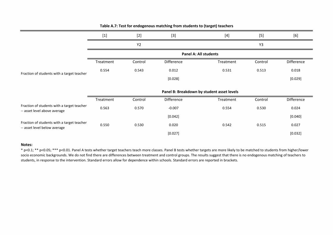
[1] [2] [3] [4] [5] [6]

Treatment Control Difference Treatment Control Difference

Fraction of students with a target teacher0.554 0.543 0.012 0.531 0.513 0.018

[0.028] [0.029]

Treatment Control Difference Treatment Control Difference

Fraction of students with a target teacher

-- asset level above average0.563 0.570 -0.007 0.554 0.530 0.024

[0.042] [0.040]

Fraction of students with a target teacher

-- asset level below average0.550 0.530 0.020 0.542 0.515 0.027

[0.027] [0.032]

Notes:* p<0.1; ** p<0.05; *** p<0.01. Panel A tests whether target teachers teach more classes. Panel B tests whether targets are more likely to be matched to students from higher/lower

socio economic backgrounds. We do not find there are differences between treatment and control groups. The results suggest that there is no endogenous matching of teachers to

students, in response to the intervention. Standard errors allow for dependence within schools. Standard errors are reported in brackets.

Table A.7: Test for endogenous matching from students to (target) teachers

Y2 Y3

Panel A: All students

Panel B: Breakdown by student asset levels

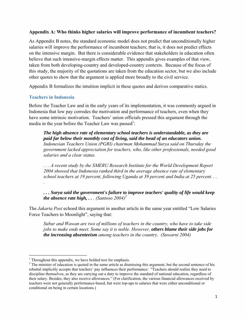
1  

Appendix A: Who thinks higher salaries will improve performance of incumbent teachers?

As Appendix B notes, the standard economic model does not predict that unconditionally higher salaries will improve the performance of incumbent teachers; that is, it does not predict effects on the intensive margin. But there is considerable evidence that stakeholders in education often believe that such intensive-margin effects matter. This appendix gives examples of that view, taken from both developing-country and developed-country contexts. Because of the focus of this study, the majority of the quotations are taken from the education sector, but we also include other quotes to show that the argument is applied more broadly to the civil service.

Appendix B formalizes the intuition implicit in these quotes and derives comparative statics.

Teachers in Indonesia

Before the Teacher Law and in the early years of its implementation, it was commonly argued in Indonesia that low pay corrodes the motivation and performance of teachers, even when they have some intrinsic motivation. Teachers’ union officials pressed this argument through the media in the year before the Teacher Law was passed1:

The high absence rate of elementary school teachers is understandable, as they are paid far below their monthly cost of living, said the head of an educators union. Indonesian Teachers Union (PGRI) chairman Mohammad Surya said on Thursday the government lacked appreciation for teachers, who, like other professionals, needed good salaries and a clear status.

. . . A recent study by the SMERU Research Institute for the World Development Report 2004 showed that Indonesia ranked third in the average absence rate of elementary school teachers at 19 percent, following Uganda at 39 percent and India at 25 percent. . . .

. . . Surya said the government's failure to improve teachers' quality of life would keep the absence rate high, . . . (Santoso 2004)2

The Jakarta Post echoed this argument in another article in the same year entitled “Low Salaries Force Teachers to Moonlight”, saying that:

Subur and Wawan are two of millions of teachers in the country, who have to take side jobs to make ends meet. Some say it is noble. However, others blame their side jobs for the increasing absenteeism among teachers in the country. (Suwarni 2004)

                                                            1 Throughout this appendix, we have bolded text for emphasis. 2 The minister of education is quoted in the same article as dismissing this argument, but the second sentence of his rebuttal implicitly accepts that teachers’ pay influences their performance: "Teachers should realize they need to discipline themselves, as they are carrying out a duty to improve the standard of national education, regardless of their salary. Besides, they also receive allowances.” (For clarification, the various financial allowances received by teachers were not generally performance-based, but were top-ups to salaries that were either unconditional or conditional on being in certain locations.)

2  

That article, too, cited the country’s high teacher absence rates. In November 2005, just before the Teacher Law was passed, “man in the street” interviews by the newspaper encountered similar arguments. See, for example, quotes from these two respondents, neither of whom was a teacher:

Especially in this day and age when the cost of living is so high, Indonesian teachers simply cannot rely on their salaries to make ends meet. That explains why many teachers look for side jobs to supplement their income. As a consequence, this hampers teachers' ability to focus on teaching. How can teachers be expected to give their best to students when they don't know where their family's next meal will come from?

How can we expect to have a better quality education system if teachers are busy looking for additional income outside their schools? While we may have poor facilities or a bad curriculum, as long as we have dedicated and creative teachers we can still have a good education system. Aristotle and Plato only needed to explain subjects in front of their students without having to bother about classrooms or other equipment. So, I believe that with good books and good teachers, we can achieve good quality education. But to get a good teacher, we must pay them enough to allow them to focus on students and the teaching process. (Jakarta Post 2005)

A World Bank report notes this argument in Indonesia, soon after the Law was passed:

Supriadi and Hoogenboom (2004) argue that low teachers’ salaries have contributed significantly to the decline in status of the profession. Given their low salaries, teachers are often forced to find part-time jobs to supplement their incomes. These part-time jobs are often in low status occupations, such as motorcycle driver, tricycle (becak) driver, street vendor, etc6 . Also, the need to seek extra income causes some teachers to neglect their teaching obligations. The high rate of teacher absenteeism demonstrates this phenomenon. (Jalal et al. 2009)

By the same token, if low pay worsens performance, it makes sense that increasing pay should improve teacher performance. And indeed this is the argument made by many. For example, another newspaper article published as the certification program was phased in asserted that:

the certification remains good news for most, if not all, teachers. They welcome the new policy with expectations that it can indeed improve their welfare. . . . . Despite all the issues and the flaws, the teacher certification program remains a hope for many people concerned with education in the country. Thanks to the promised doubled base payment, the educators will compete to improve their quality and the classic problems of welfare will no longer give them an excuse not to do their best before their students. (Maulia 2008)

Some of those involved in the planning also had high hopes for the intensive-margin effects of the salary increase:

3  

[Professor] Riyanto, who helped the Education and Culture Ministry design the procedure for the teacher certification program in 2008, admitted that the program’s results failed to meet his expectations. “We initially assumed that a salary increase would encourage teachers to perform better in schools. However, it turned out that most certified teachers have done almost nothing to improve their [teaching] skills or competency, making them no different than uncertified ones,” he recently told The Jakarta Post. (Widhiarto 2014)

Teachers in the global education discussion

It is not only in Indonesia that we find this argument that low salaries worsen teachers’ motivation and the quality of their teaching, and that conversely higher salaries will improve teaching. At the global level, the same argument appears in numerous recent reports.

The International Labour Organisation’s “Handbook of good human resource practices in the teaching profession” gives two rationales for setting teacher compensation high enough, which we can recognize as encompassing both the extensive-margin and intensive-margin rationales for higher pay:

“All countries need to provide teachers with rewards which meet the two equally important strategic objectives mentioned above: (1) the recruitment, retention and performance needs as defined by the relevant education authority; and (2) the incentives for individuals to become and remain teachers over the full length of a professional career as defined by the education system, as well as foster dedication to professional responsibilities by enabling teachers and their dependants to live in dignity without taking second jobs. . . . .

Together with a tendency for late or non payment of teachers‘ salaries, these are amongst the factors which lead teachers in many countries to take on second jobs, to the detriment of their teaching, morale and well being, or to leave teaching altogether. (ILO 2012)

UNICEF’s report on Protecting Salaries of Frontline Teachers and Healthcare Workers argues that:

Studies suggest that low pay is a key factor behind teacher absenteeism, informal fees, and brain drain, which in turn is a cause for poor child outcomes especially in rural areas. For example, staff absenteeism in the early 2000s was as high as 35 percent in rural Bangladesh, Lesotho, Ghana, Mozambique and Zambia . . . . (UNICEF 2010)

The report proposes as one policy response:

Paying attention to real pay levels to ensure that compensation keeps up with increases in the cost of living in order to minimize the risk of staff absenteeism, brain drain and coping strategies such as informal fees.

4  

Similarly, the UNESCO “Methodological Guide for the Analysis of Teacher Issues” says that:

Status, career, and salary issues all have an impact on the attractiveness of the teaching profession, and therefore on the profile of new teachers, their motivation once hired, as well as on teacher attrition and the social context. Absenteeism levels are also influenced both by teacher motivation and by the dispositions through which the teacher has been hired . . . .

UNESCO’s Global Monitoring Report 2009 (UNESCO 2009), although focused on governance issues, also reflects this view of intensive-margin effects:

In Malawi, average teacher salaries are too low to meet basic needs. There, and in many other countries, teachers often have to supplement their income with a second job, with damaging consequences for the quality of their teaching. . . .

Poor morale and weak motivation undermine teacher effectiveness. Teacher retention and absenteeism and the quality of teaching are heavily influenced by whether teachers are motivated and their level of job satisfaction. Evidence suggests many countries face a crisis in teacher morale that is mostly related to poor salaries, working conditions and limited opportunities for professional development (Bennell and Akyeampong, 2007; DFID and VSO, 2008). . . .

One consequence of low relative pay in Central Asia has been an increase in the number of teachers seeking to supplement their income through a second job – a phenomenon that has been extensively documented in most Central Asian countries (Education Support Program, 2006). This practice can have damaging consequences for the quality of education, with some teachers withholding curriculum to pressure students into private tutoring (Bray, 2003).

Similarly, the Global Monitoring Report 2014 (UNESCO 2014) notes that

[w\hen salaries are too low, teachers often need to take on additional work – sometimes including private tuition – which can reduce their commitment to their regular teaching jobs and lead to absenteeism.

It is important to stress that these reports by international organizations all advocate multipronged approaches to improving teacher performance. None expresses the belief that raising salaries alone will be enough. Yet in each case, embedded somewhere in the argument is the view that salary increases and decreases have intensive-margin effects on the quality of teaching, as these quotes show.

Teachers in other countries

We encounter this argument at the country level in countries other than Indonesia as well.

In the United States, advocates for raising teacher pay commonly cite these intensive-margin effects on teachers’ ability to better serve their students. A San Francisco Chronicle opinion piece by the co-founder of Teacher Salary Project (TSP) argues that

5  

Teachers want to give their all, but being financially stressed and moonlighting does not allow them to teach their best. (Calegari 2015)

To bring this problem alive, the TSP has produced a short documentary about Laney,

a public middle school teacher who works two after-school jobs and spends her nights bartending just so she can afford to stay in the classroom. Laney fears she won’t make enough to pay her bills—and fears even more that she can’t give 100 percent to her students because she is so over-worked and exhausted. . . .

If teachers like Laney were appropriately compensated they would no longer need to work two and three jobs outside of the classroom. Instead of struggling to pay rent, they would be able to fully devote themselves to our nation’s children.

“It makes me really upset to think I’m not giving them my best,” Laney says in the film. (Teacher Salary Project 2015)

In Peru, a survey and study of teachers finds that they too argue that low pay inhibits performance:

77.5 per cent of the Peruvian teachers interviewed consider that they are “badly” or “very badly” paid. Very often, they need to complement their income with other jobs, which results in less time available for lesson preparation and a focus on teaching. Better salaries could benefit the professionalisation of teaching and would allow teachers to focus more on their careers. (van der Tuin and Verger 2013)

In Ethiopia, teachers surveyed for a study also make this argument:

The issues raised by the research were numerous, but the most significant and most often-mentioned causes of demotivation and low morale were: • inadequate salaries • low respect for and low status of teachers • poor management and leadership. These issues have a significant impact on classroom performance, that is, teachers’ ability to deliver good quality education, as well as on levels of teacher retention.

In the case of Cambodia, an NGO study (VSO 2008) cited by some international agencies recommends:

[i]ncreasing the salaries of teachers, school directors and staff of the provincial and district offices of education to a level appropriate to the cost of living and linked to inflation. In every focus group conducted with teachers, the issue of pay emerged as the most powerful de-motivating factor. It is impossible to earn a living on a teacher’s salary in Cambodia. This basic need is going to remain the top priority over and above any other aspirations teachers have for the quality of their teaching practice until it is fulfilled.

It goes on to say that

a reasonable salary would make the pressure to earn a living wage less intense, which should have a positive effect on teachers’ commitment and practice. (VSO 2008)

6  

And in the case of the Caucasus and Central Asia, UNICEF (2011) finds that

The need to rely on additional income from economic activities outside of school applies specifically to teachers in rural areas. . . . . [T]eacher absences during harvesting season are common and tolerated by the school and the community. For a few weeks of the year, the second job absorbs so much of the teachers’ time that they temporarily redefine their professional identities and primarily see themselves as farmers or merchants, and only secondarily as teachers with a part-time teaching job at school.

Other civil servants

Similar intensive-margin arguments have been made for other civil servants in Indonesia. One argument is that (consistent with model 3 in Appendix B) because civil servants’ salaries have been seen as too low, the Indonesian government has not been able to enforce standards of performance. Commenting on a 2009 Law on Public Services, one scholar writes that

Enforcement of the sanctions contained in the law implicitly takes for granted the power of senior bureaucrats within the state apparatus. This may not accurately reflect the power dynamics within Indonesian public service providers. Examining power relations within the bureaucracy more than three decades ago, one observer noted:

In their routine efforts to gather information, implement decisions, and mobilize employees, superiors were faced with the fact that they often did not have sufficient authority to do these things ... [Civil servants often argued] to outsiders, and to themselves, that because government salaries were so low, superiors did not have a right to demand more than a minimum of obedience from them ... It was recognized at the top, just as it was widely claimed at the bottom, that the government did not have the right to demand more than semi-obedience and half-effort ... On paper, Indonesian superiors ... had the power to act against transgressors and to require subordinates to work every hour of each day, but it was recognized by everyone that what was written down was not conceded in fact, and that it would be futile to act as if it were. The natural response of employees who suffered cuts in honoraria or incentive money was to work less ... The incapacity, or extreme reluctance, of superiors to punish transgressions occurring at others’ or even their own expense permitted a chronic crisis of authority to infect every pore of the government bureaucracy. The result was to work at a snail’s pace or, commonly, not to work at all (Conkling 1979: 443–550)

. . . . Weak authority among superiors is likely to persist despite the nominal availability of formal means of punishment, as civil servants will continue to seek refuge in the rhetoric of insubordination because of low pay. (Buehler 2011)

Many Indonesians believe that higher salaries should reduce corruption, while also improving performance along other dimensions. Note that some aspects of poor teacher performance –

7  

such as excessive absenteeism – straddle the line between underperformance and corruption, and so would be covered by both avenues for improving performance:

“Appropriate compensation will not only have an impact on staff turnover and on employees’ productivity and quality of work, but will also reduce tendencies for civil servants to engage in corrupt practices.” (Tjiptoherijanto 2008)

A survey of business executives, household, and civil servants in Indonesia published in 2000, several years before the Teacher Law of 2005, showed that this view was widely shared:

“Respondents were asked to rank the main causes of corruption in society from amongst a list of possible reasons. The results showed a strong consensus among all three groups with more than one-third of households (36%) and business enterprises (37%) attributing the main cause of corruption to low civil servant salaries. Public officials were even more strongly of this view with over half of them (51%) putting this reason first.

. . . . almost half of the public officials reported receiving unofficial payments. The argument that low salaries are a cause of corruption assumes that wages are inadequate to meet daily needs, and thus income has to be supplemented with bribes.” (Partnership for Governance Reform3 2000)

The report’s authors go on to challenge this assumption, saying “While low salaries as a cause of corruption may be the most widely held belief, the accuracy of this relationship is disputed in the corruption research literature.” Nevertheless, a view that was so prevalent may have contribute to the legislature’s decision to raise teacher salaries.

This argument that higher (unconditional) salaries lead to better civil-servant performance is not unique to Indonesia either. In the case of Cambodia, Korm (2011) argues that:

The prevailing opinion is that the low incomes of public servants have led them to pay too little attention to their official tasks and duties as they have diverted their time and effort to obtaining additional sources of income. They have become involved in corruption and „moonlighting‟ in other jobs. Furthermore, it is thought that public servants have rationalised such behaviour using the argument that low pay justifies their poor performance. Whatever the reason, public service delivery is thought to have suffered significantly . . . .

In Cambodia, civil servants are paid sums that cannot support a decent standard of living. Securing adequate income may then become the first priority in their minds as they need to meet their necessary costs of living. Chew (1997) emphasised that if civil servants were well paid in relation to the cost of living, their performance would be good because they could concentrate on their work. When they are paid reasonably, they are happy and they perform to the required standard without being constantly

                                                            3 This partnership included the World Bank, United Nations Development Program, the Asian Development Bank (ADB), and a Governing Board comprising “a number of reform minded individuals including ministers, senior public officials and private entrepreneurs.”

8  

concerned about finding more money to support their living. However, where public servants’ pay is very low in relation to the cost of living, their productivity and quality of performance are similarly low.

As Korm points out, McCourt (2003), in his Global Human Resource Management book, summarizes this situation using the old joke: “you pretend to pay us, and we pretend to work.” Describing the situation in “many developing and transitional countries”, McCourt says that as a result,

It is difficult for a supervisor to criticize an employee’s poor attendance record when the supervisor knows that it is almost forced on the employee (and supervisors are probably in the same position themselves).

Appendix B: Theoretical framework

In this section, we develop three classes of models that illustrate possible mechanisms through which an unconditional salary increase on the primary teaching job could increase a teacher’s effort on that job. The models are extensions of a standard model where, as the salary on primary job is unrelated to performance, the teacher will always exert the minimum level of effort. We extend this model by recognizing that (1) teaching is a pro-social task from which teachers could derive utility through the learning gains they contribute to (2) there maybe reciprocity and gift exchange in employment contracts (Akerlof 1982; Fehr and Gachter 2000) and (3) communities and administrators may provide non-pecuniary sanctions or rewards based on actual performance relative to expectations (Webb and Valencia 2006, Cotlear 2006). The standard model We assume that salary ( ) on the primary teaching job is not dependent on performance, and

that employment contracts are guaranteed as long as a minimum amount of effort ( is

provided (where the p indexes the primary job). This minimum level of effort may exceed the effort threshold at which the teacher would be dismissed, because the teacher is assumed to have some level of professionalism or intrinsic motivation (varying across individuals) that sets his or her default level of effort under low-powered incentives (as in Holmstrom and

Milgrom 1991). Thus, the ( could vary across teachers and should be thought of as the

default level of teacher effort when there are no financial incentives. We also allow for the possibility of secondary jobs. Secondary jobs pay a piece-rate wage ( ) for each unit of effort ( ). Workers are endowed with a fixed amount of effort ( , which they can distribute over effort on the primary job ( , on the secondary job ( ), and on leisure ( .1 (B.1) In this standard setup, a worker derives utility from consumption—which in this static framework (we abstract from savings) is assumed to be equal to total earnings derived from the primary and secondary jobs—and from the effort that is devoted to leisure, . The utility functions and are worker-specific with standard properties. Substituting the effort constraint for , the utility function of the teacher is (B.2)

1 We prefer to model effort allocation rather than time allocation, since time spent at school does not necessarily imply that effort is put into making children learn. Teachers could be away from their classroom chatting with their colleagues, and in fact fieldwork shows that this phenomenon of “shirking while at work” is quantitatively important in some settings, as in India and Indonesia (Kremer et al 2005, McKenzie et al 2014). We would consider this as effort spent on leisure.

In this setting, the teacher will work at his or her default effort level ( on the primary

job. Extra effort beyond this level provides no additional income and reduces leisure. Further, in this standard model, an unconditional increase in salary will lead to a reduction in hours spent on the secondary job, an increase in leisure, and no change in ( , consistent with a positive income elasticity of leisure. We introduce three possible extensions of this standard model, each of which yields an increase in effort on the primary teaching job in response to an unconditional increase in salary . As discussed in the text, our policy experiment does not correspond to a precise test of any of these particular extensions. Rather, our aim is to illustrate the theoretical models of worker behavior that predict increased teacher effort in response to an unconditional increase in base salary. Pro-social preferences The first extension is to assume that the teacher also derives utility from her contribution to the human capital (ΔHC) of students in her classroom. In other words, the teacher is assumed to have pro-social preferences (Levitt and List 2007). While not all workers may exhibit such preferences, it is widely believed that teachers partly select into their jobs because they hold such preferences. We model utility from pro-social preferences as Δ (B.3) where HC is the human capital accumulated by children in the classroom of the teacher, and is assumed to depend positively on the effort exerted by the teacher on her primary job: Δ (B.4) We assume that either one or both of and have decreasing marginal returns to inputs (and

that neither has increasing returns). Hence, the reduced form also has positive and decreasing marginal returns with respect to effort on the primary teaching job: (B.5)

With this addition to the standard model, a teacher with pro-social preferences would

typically exert more than the default minimum effort on the primary teaching job,

because she derives utility from contributing to learning of children.2 It is easy to see how such a set-up generates a positive income elasticity of effort on the primary teaching job. Basically, there are now two kinds of effort: "grunt" work ( ) that yields no intrinsic utility and is only done for income (and the consumption made possible by

2 The main reason for not incorporating the variation in the extent of pro-social preferences into the variation in the teacher's default effort is that pro-social preferences generate a positive income elasticity of effort on the pro-social task, whereas variation in the teacher's default effort level due to variation in their effort norms will not.

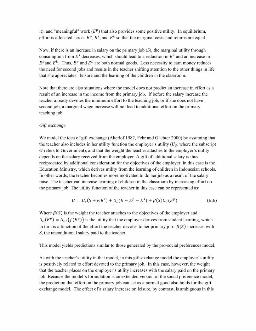
it), and "meaningful" work ( ) that also provides some positive utility. In equilibrium, effort is allocated across , , and so that the marginal costs and returns are equal. Now, if there is an increase in salary on the primary job (S), the marginal utility through consumption from decreases, which should lead to a reduction in and an increase in

and . Thus, and are both normal goods. Less necessity to earn money reduces the need for second jobs and results in the teacher shifting attention to the other things in life that she appreciates: leisure and the learning of the children in the classroom. Note that there are also situations where the model does not predict an increase in effort as a result of an increase in the income from the primary job. If before the salary increase the teacher already devotes the minimum effort to the teaching job, or if she does not have second job, a marginal wage increase will not lead to additional effort on the primary teaching job. Gift exchange We model the idea of gift exchange (Akerlof 1982, Fehr and Gächter 2000) by assuming that the teacher also includes in her utility function the employer’s utility ( ,where the subscript G refers to Government), and that the weight the teacher attaches to the employer’s utility depends on the salary received from the employer. A gift of additional salary is thus reciprocated by additional consideration for the objectives of the employer, in this case is the Education Ministry, which derives utility from the learning of children in Indonesian schools. In other words, the teacher becomes more motivated to do her job as a result of the salary raise. The teacher can increase learning of children in the classroom by increasing effort on the primary job. The utility function of the teacher in this case can be represented as:

(B.6)

Where is the weight the teacher attaches to the objectives of the employer and

is the utility that the employer derives from student learning, which

in turn is a function of the effort the teacher devotes to her primary job. increases with S, the unconditional salary paid to the teacher. This model yields predictions similar to those generated by the pro-social preferences model. As with the teacher’s utility in that model, in this gift-exchange model the employer’s utility is positively related to effort devoted to the primary job. In this case, however, the weight that the teacher places on the employer’s utility increases with the salary paid on the primary job. Because the model’s formulation is an extended version of the social preference model, the prediction that effort on the primary job can act as a normal good also holds for the gift exchange model. The effect of a salary increase on leisure, by contrast, is ambiguous in this

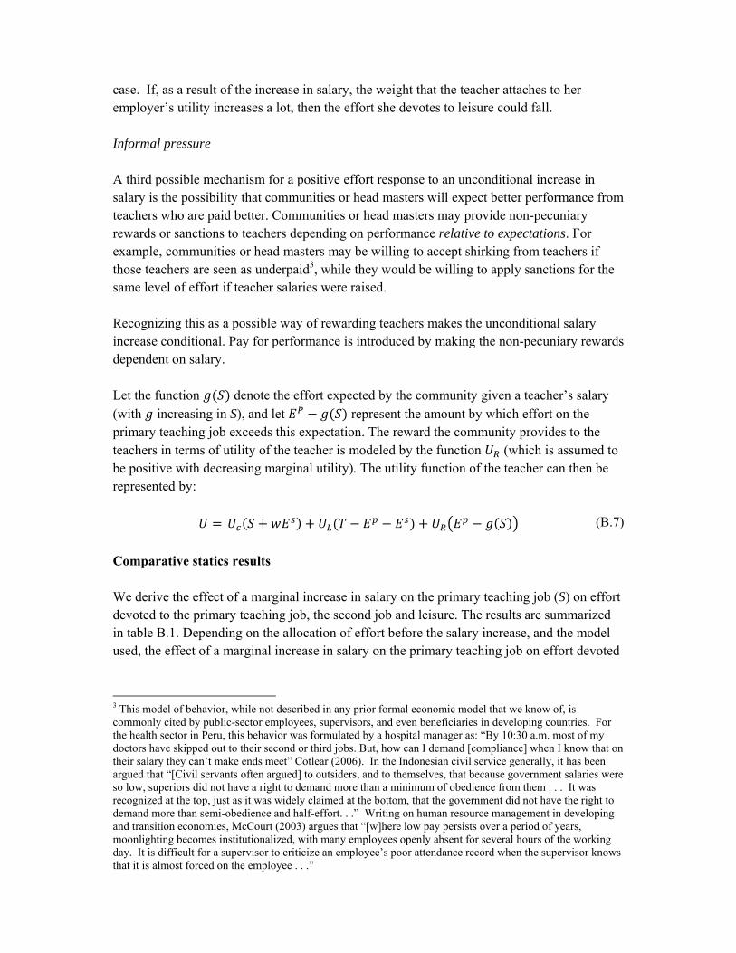
case. If, as a result of the increase in salary, the weight that the teacher attaches to her employer’s utility increases a lot, then the effort she devotes to leisure could fall. Informal pressure A third possible mechanism for a positive effort response to an unconditional increase in salary is the possibility that communities or head masters will expect better performance from teachers who are paid better. Communities or head masters may provide non-pecuniary rewards or sanctions to teachers depending on performance relative to expectations. For example, communities or head masters may be willing to accept shirking from teachers if those teachers are seen as underpaid3, while they would be willing to apply sanctions for the same level of effort if teacher salaries were raised. Recognizing this as a possible way of rewarding teachers makes the unconditional salary increase conditional. Pay for performance is introduced by making the non-pecuniary rewards dependent on salary. Let the function denote the effort expected by the community given a teacher’s salary (with increasing in S), and let represent the amount by which effort on the primary teaching job exceeds this expectation. The reward the community provides to the teachers in terms of utility of the teacher is modeled by the function (which is assumed to be positive with decreasing marginal utility). The utility function of the teacher can then be represented by: (B.7)

Comparative statics results We derive the effect of a marginal increase in salary on the primary teaching job (S) on effort devoted to the primary teaching job, the second job and leisure. The results are summarized in table B.1. Depending on the allocation of effort before the salary increase, and the model used, the effect of a marginal increase in salary on the primary teaching job on effort devoted

3 This model of behavior, while not described in any prior formal economic model that we know of, is commonly cited by public-sector employees, supervisors, and even beneficiaries in developing countries. For the health sector in Peru, this behavior was formulated by a hospital manager as: “By 10:30 a.m. most of my doctors have skipped out to their second or third jobs. But, how can I demand [compliance] when I know that on their salary they can’t make ends meet” Cotlear (2006). In the Indonesian civil service generally, it has been argued that “[Civil servants often argued] to outsiders, and to themselves, that because government salaries were so low, superiors did not have a right to demand more than a minimum of obedience from them . . . It was recognized at the top, just as it was widely claimed at the bottom, that the government did not have the right to demand more than semi-obedience and half-effort. . .” Writing on human resource management in developing and transition economies, McCourt (2003) argues that “[w]here low pay persists over a period of years, moonlighting becomes institutionalized, with many employees openly absent for several hours of the working day. It is difficult for a supervisor to criticize an employee’s poor attendance record when the supervisor knows that it is almost forced on the employee . . .”  

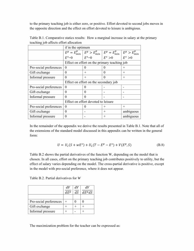
to the primary teaching job is either zero, or positive. Effort devoted to second jobs moves in the opposite direction and the effect on effort devoted to leisure is ambigious. Table B.1. Comparative statics results: How a marginal increase in salary at the primary teaching job affects effort allocation if in the optimum

=0

=0

0

0 Effect on effort on the primary teaching job Pro-social preferences 0 0 0 + Gift exchange 0 + 0 + Informal pressure 0 + 0 + Effect on effort on the secondary job Pro-social preferences 0 0 - - Gift exchange 0 0 - - Informal pressure 0 0 - - Effect on effort devoted to leisure Pro-social preferences 0 0 + + Gift exchange 0 - + ambiguous Informal pressure 0 - + ambiguous In the remainder of the appendix we derive the results presented in Table B.1. Note that all of the extensions of the standard model discussed in this appendix can be written in the general form: , (B.8) Table B.2 shows the partial derivatives of the function W, depending on the model that is chosen. In all cases, effort on the primary teaching job contributes positively to utility, but the effect of salary varies depending on the model. The cross-partial derivative is positive, except in the model with pro-social preference, where it does not appear. Table B.2. Partial derivatives for W

Pro-social preferences + 0 0 Gift exchange + + + Informal pressure + - + The maximization problem for the teacher can be expressed as:

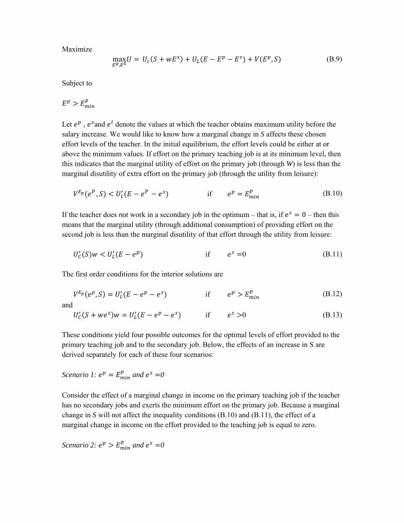
Maximize max

, , (B.9)

Subject to

Let , and denote the values at which the teacher obtains maximum utility before the salary increase. We would like to know how a marginal change in S affects these chosen effort levels of the teacher. In the initial equilibrium, the effort levels could be either at or above the minimum values. If effort on the primary teaching job is at its minimum level, then this indicates that the marginal utility of effort on the primary job (through W) is less than the marginal disutility of extra effort on the primary job (through the utility from leisure): , if (B.10)

If the teacher does not work in a secondary job in the optimum – that is, if 0 – then this means that the marginal utility (through additional consumption) of providing effort on the second job is less than the marginal disutility of that effort through the utility from leisure: if 0 (B.11) The first order conditions for the interior solutions are , if (B.12)

and if 0 (B.13) These conditions yield four possible outcomes for the optimal levels of effort provided to the primary teaching job and to the secondary job. Below, the effects of an increase in S are derived separately for each of these four scenarios:

Scenario 1: and 0

Consider the effect of a marginal change in income on the primary teaching job if the teacher has no secondary jobs and exerts the minimum effort on the primary job. Because a marginal change in S will not affect the inequality conditions (B.10) and (B.11), the effect of a marginal change in income on the effort provided to the teaching job is equal to zero.

Scenario 2: and 0

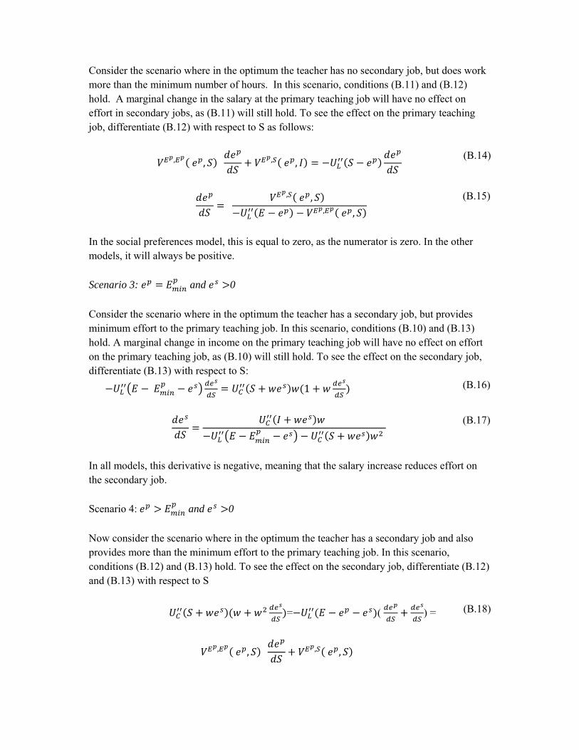
Consider the scenario where in the optimum the teacher has no secondary job, but does work more than the minimum number of hours. In this scenario, conditions (B.11) and (B.12) hold. A marginal change in the salary at the primary teaching job will have no effect on effort in secondary jobs, as (B.11) will still hold. To see the effect on the primary teaching job, differentiate (B.12) with respect to S as follows: , , , ,

(B.14)

, ,

, ,

(B.15)

In the social preferences model, this is equal to zero, as the numerator is zero. In the other models, it will always be positive.

Scenario 3: and 0

Consider the scenario where in the optimum the teacher has a secondary job, but provides minimum effort to the primary teaching job. In this scenario, conditions (B.10) and (B.13) hold. A marginal change in income on the primary teaching job will have no effect on effort on the primary teaching job, as (B.10) will still hold. To see the effect on the secondary job, differentiate (B.13) with respect to S: 1 (B.16)

(B.17)

In all models, this derivative is negative, meaning that the salary increase reduces effort on the secondary job.

Scenario 4: and 0

Now consider the scenario where in the optimum the teacher has a secondary job and also provides more than the minimum effort to the primary teaching job. In this scenario, conditions (B.12) and (B.13) hold. To see the effect on the secondary job, differentiate (B.12) and (B.13) with respect to S = ( ) =

, , , ,

(B.18)

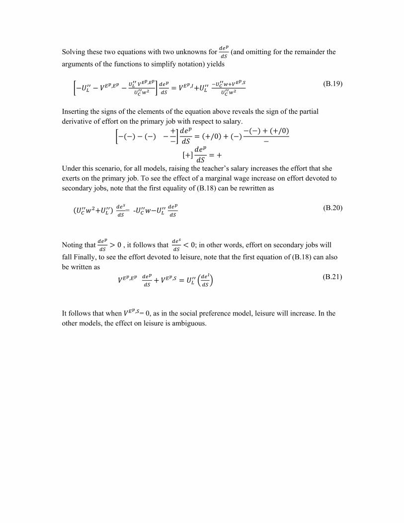
Solving these two equations with two unknowns for (and omitting for the remainder the

arguments of the functions to simplify notation) yields , ,

,,

(B.19)

Inserting the signs of the elements of the equation above reveals the sign of the partial derivative of effort on the primary job with respect to salary.

/0/0

Under this scenario, for all models, raising the teacher’s salary increases the effort that she exerts on the primary job. To see the effect of a marginal wage increase on effort devoted to secondary jobs, note that the first equality of (B.18) can be rewritten as = -

(B.20)

Noting that 0 , it follows that 0; in other words, effort on secondary jobs will

fall Finally, to see the effort devoted to leisure, note that the first equation of (B.18) can also be written as , ,

(B.21)

It follows that when , = 0, as in the social preference model, leisure will increase. In the other models, the effect on leisure is ambiguous.

References for Appendix A and Appendix B BUEHLER, M. (2011): "Indonesia's Law on Public Services: Changing State-Society Relations or

Continuing Politics as Usual?," Bulletin of Indonesian Economic Studies, 47 1, 65-86. CALEGARI, N. (2015): "Why Do Teachers Need Side Jobs to Pay Bills?." HOLMSTROM, B., and P. MILGROM (1991): "Multitask Principal-Agent Analyses: Incentive Contracts,

Asset Ownership, and Job Design," Journal of Law, Economics, and Organization, 7, 24-52. ILO (2012): Handbook of Good Human Resource Practices in the Teaching Profession. Geneva:

International Labour Organization. JAKARTA POST (2005): "'Most Teachers Are Gravely Underpaid'." JALAL, F., M. SAMANI, M. C. CHANG, R. STEVENSON, A. B. RAGATZ, and S. D. NEGARA (2009):

"Teacher Certification in Indonesia: A Strategy for Teacher Quality Improvement," Jakarta: World Bank.

KORM, R. (2011): "The Relationship between Pay and Performance in the Cambodian Civil Service," Doctoral thesis, University of Canberra.

KREMER, M., K. MURALIDHARAN, N. CHAUDHURY, F. H. ROGERS, and J. HAMMER (2005): "Teacher Absence in India: A Snapshot," Journal of the European Economic Association, 3, 658-67.

MAULIA, E. (2008): "Teacher Certification a Hope Amid Concerns About Quality ". MCCOURT, W., and D. ELDRIDGE (2003): Global Human Resource Management: Managing People in

Developing and Transitional Countries. Cheltenham, U.K. and Northampton, Mass.: Elgar. MCKENZIE, P., D. NUGROHO, C. OZOLINS, J. MCMILLAN, S. SUMARTO, N. TOYAMAH, V. FEBRIANY, R.

J. SODO, L. BIMA, and A. A. SIM (2014): "Study on Teacher Absenteeism in Indonesia 2014," Jakarta : Education Sector Analytical and Capacity Development Partnership (ACDP).

PARTNERSHIP FOR GOVERNANCE REFORM (2000): "A Diagnostic Study of Corruption in Indonesia," Jakarta.

SANTOSO, D. (2004): "Govt Expects Too Much from Poverty-Line Teachers: Union." SUWARNI (2004): "Low Salaries Force Teacher to Moonlight." TEACHER SALARY PROJECT (2015): "New Short Documentary Reveals Tradeoffs of Teachers’ Second

Jobs: Teacher Salary Project Continues Push for Equity, Professionalism." TJIPTOHERIJANTO, P. (2008): "Civil Service Reform in Indonesia," Emerald Group Publishing Limited,

39-53 UNESCO (2009): Efa Global Monitoring Report 2009. Overcoming Inequality: Why Governance

Matters. Paris: UNESCO. — (2010): "Methodological Guide for the Analysis of Teacher Issues," Teacher Training Initiative for

Sub-Saharan Africa (TTISSA) Teacher Policy Development Guide. — (2014): Teaching and Learning: Achieving Quality for All. Efa Global Monitoring Report 2013/14. .

Paris, France: UNESCO. UNICEF (2010): "Social and Economic Policy Working Brief: Protecting Salaries of Frontline Teachers

and Health Workers," UNICEF. — (2011): Teachers: A Regional Study on Recruitment, Development and Salaries of Teachers in the

Ceecis Region. Geneva: UNICEF. VAN DER TUIN, M., and A. VERGER (2013): "Evaluating Teachers in Peru: Policy Shortfalls and Political

Implications," in Global Managerial Education Reforms and Teachers: Emerging Policies, Controversies and Issues in Developing Countries, ed. by A. Verger, H. K. Altinyelken, and M. de Koning: Education International Research Institute.

VSO (2008): "Teaching Matters: A Policy Report on the Motivation and Morale of Teachers in Cambodia," London: VSO International.

— (2010): "How Much Is a Good Teacher Worth? A Report on the Motivation and Morale of Teachers in Ethiopia," London: VSO International.

WIDHIARTO, H. (2014): "Amid Soaring Education Budget, Performance Remains Low."