2000/14 October 2000 Documents

Statistics NorwayResearch Department

Hilde Christiane Bjørnland

VAR Models in MacroeconomicResearch

-869:1 71:1 73:1 75:1 77:1 79:1 81:1 83:1 85:1 87:1 89:1 91:1 93:1

-USAGERMANY

- UK6 4-

-USAGERMANY

--- UK

2.

69:1 71:1 73:1 75:1 77:1 79:1 81:1 83:1 85:1 87:1 89:1 91:1 93:10

12 7

10

8

6

- NORWAY

10 T

-1

7 T.

5 4-

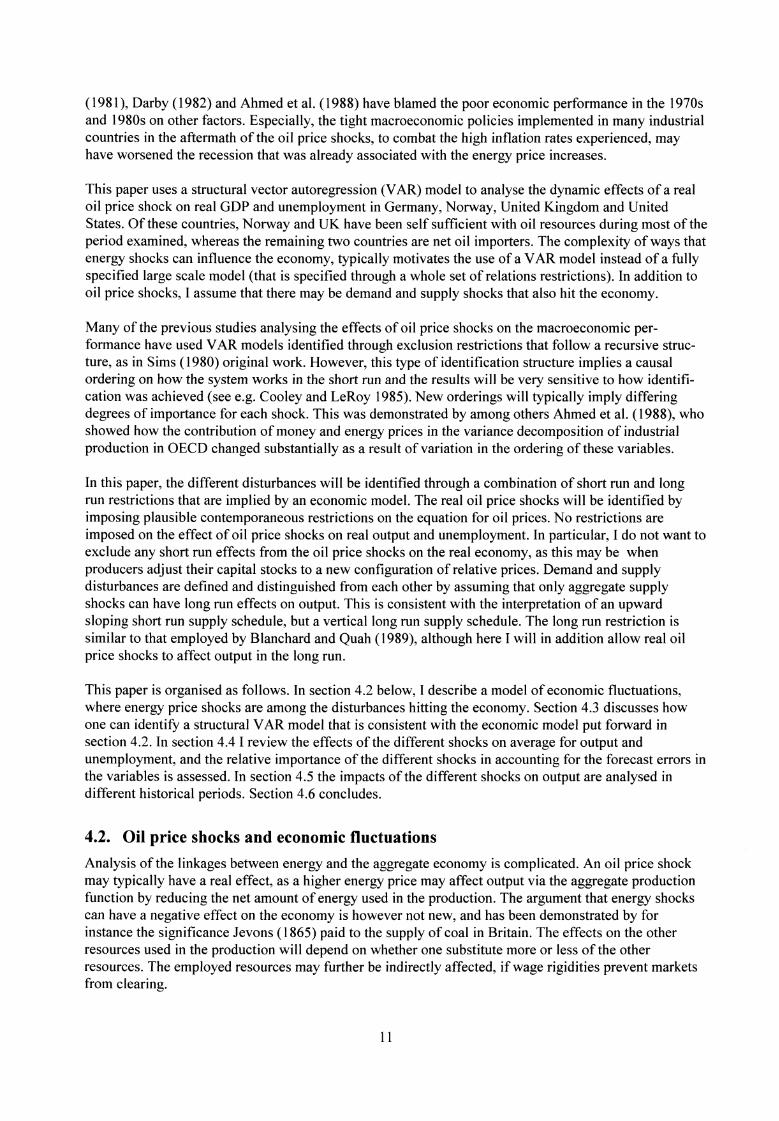
1. IntroductionThe study of possible sources of economic fluctuations has been the major preoccupation inmacroeconomics in recent years. The question is fundamental if one shall gain insight into the workingsof the economy, and aid in the formulation and conduct of economic policy. Earlier empirical studiesaddressing the sources of aggregate economic variability in the Norwegian economy have typically beenconducted using large scale models (or partial econometric analysis). Here I draw on recentdevelopments in modern business cycle research and econometric methodology and discuss how one cananalyse business cycles with the aid of complete, yet small and transparent systems.

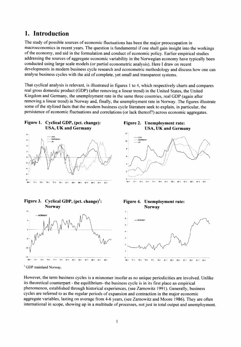
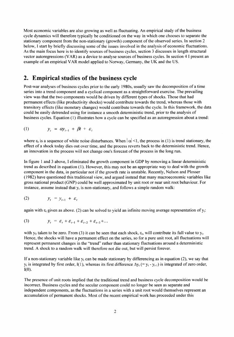
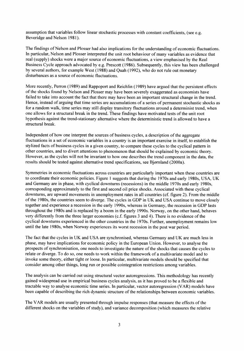
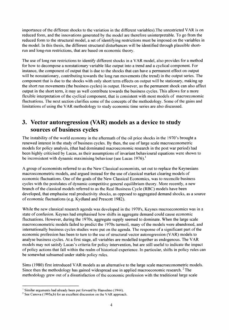
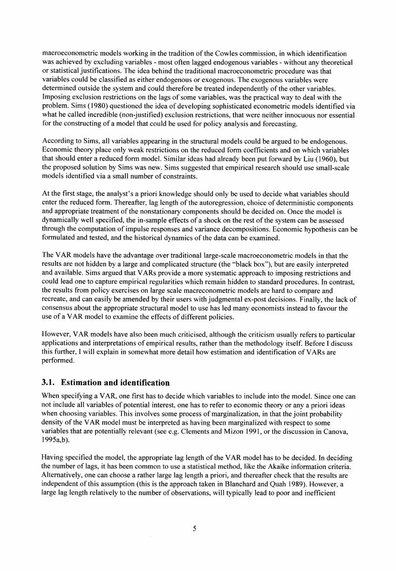
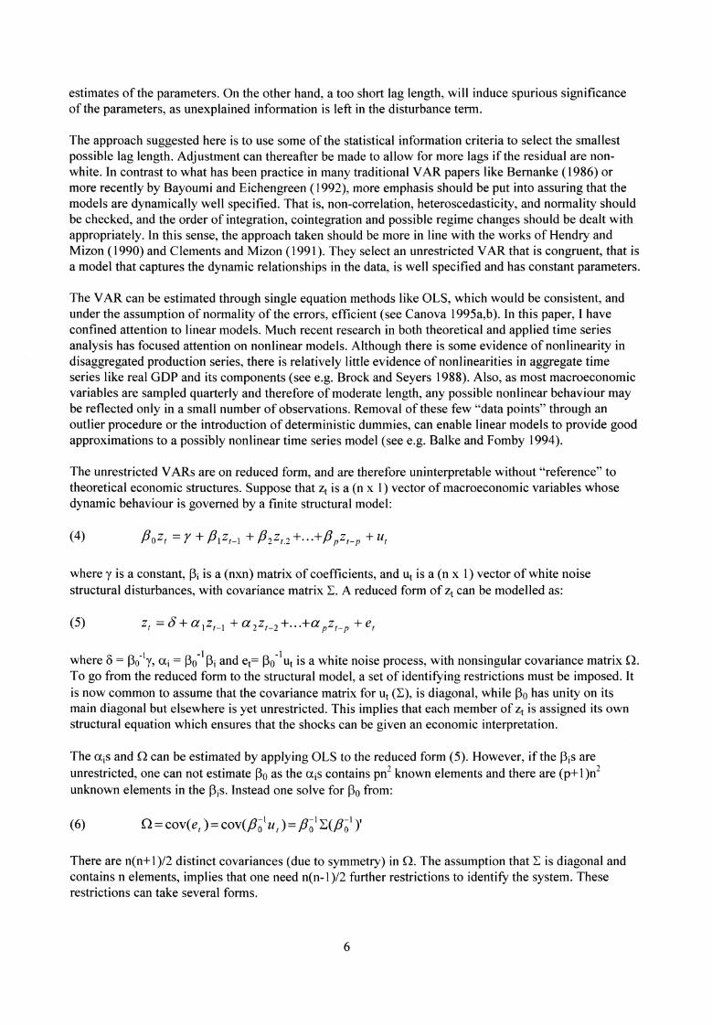
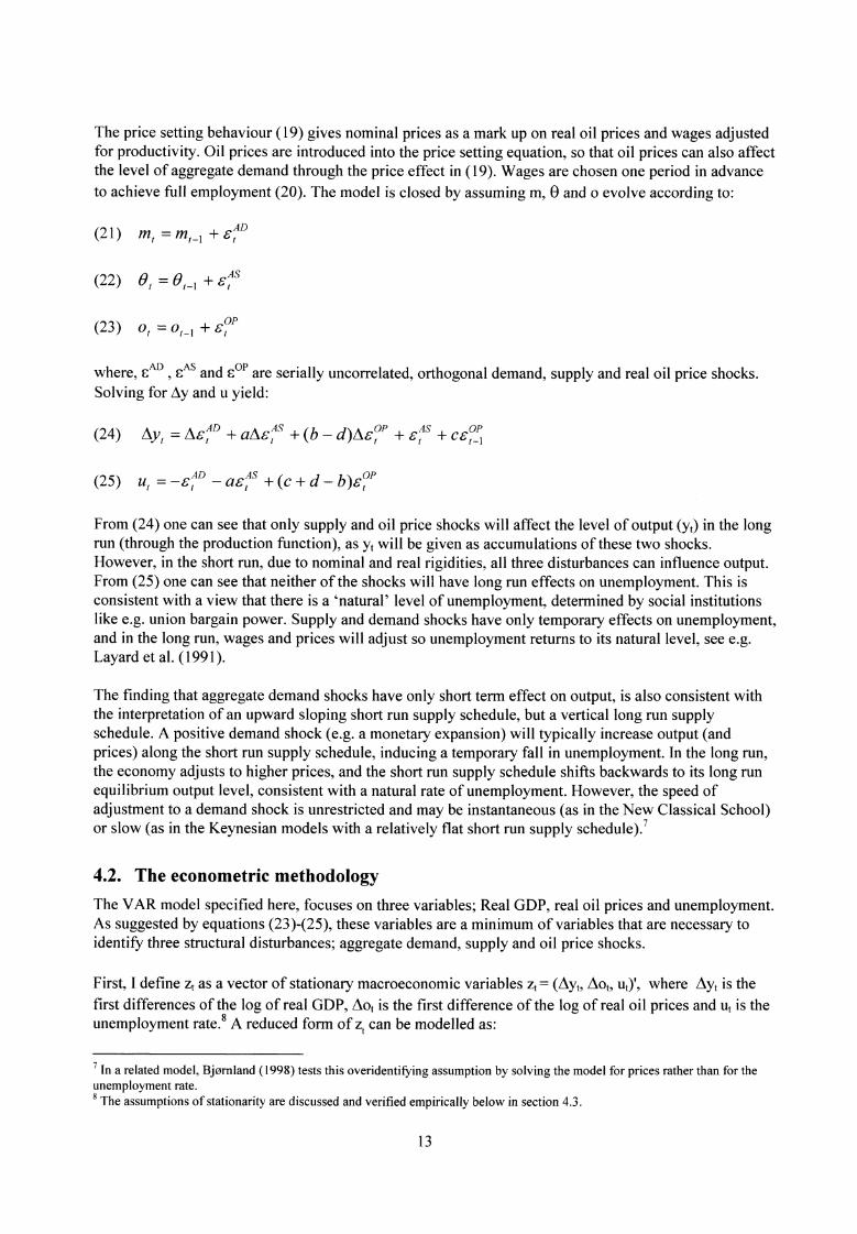
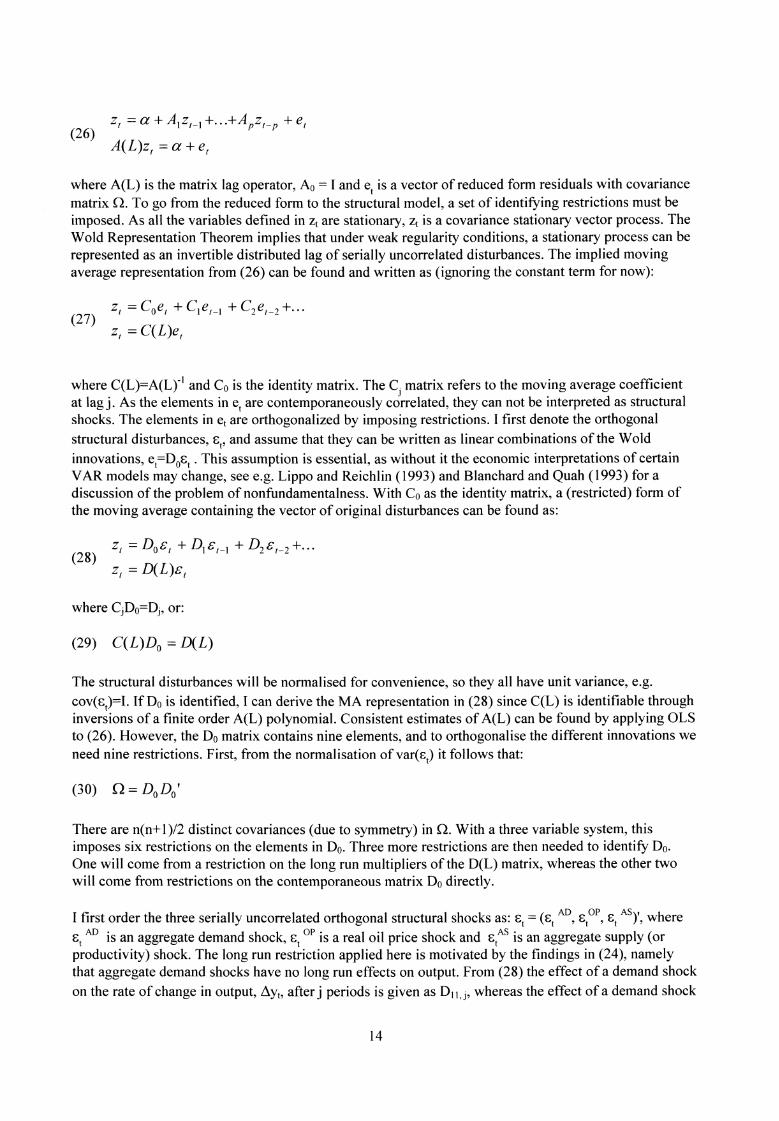
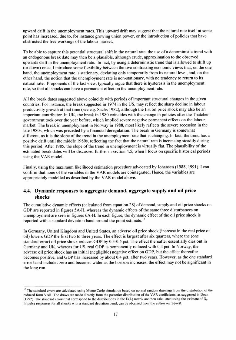
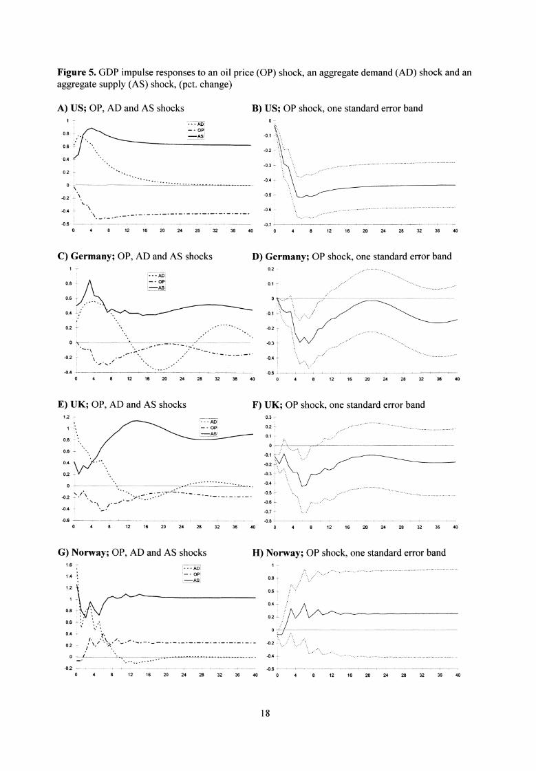
That cyclical analysis is relevant, is illustrated in figures 1 to 4, which respectively charts and comparesreal gross domestic product (GDP) (after removing a linear trend) in the United States, the UnitedKingdom and Germany, the unemployment rate in the same three countries, real GDP (again afterremoving a linear trend) in Norway and, finally, the unemployment rate in Norway. The figures illustratesome of the stylized facts that the modern business cycle literature seek to explain, in particular, thepersistence of economic fluctuations and correlations (or lack thereof?) across economic aggregates.

Figure 1. Cyclical GDP, (pct. change):USA, UK and Germany

Figure 2. Unemployment rate:USA, UK and Germany

Figure 3. Cyclical GDP, (pct. change)': Figure 4. Unemployment rate:Norway Norway

-15 69:1 71:1 73:1 75:1 77:1 79:1 81:1 83:1 85:1 87:1 89:1 91:1 93:1

I GDP mainland Norway.

69:1 71:1 73:1 75:1 77:1 79:1 81:1 83:1 85:1 87:1 89:1 91:1 93:1

However, the term business cycles is a misnomer insofar as no unique periodicities are involved. Unlikeits theoretical counterpart - the equilibrium- the business cycle is in its first place an empiricalphenomenon, established through historical experiences, (see Zarnowitz 1991). Generally, businesscycles are referred to as the regular periods of expansion and contraction in the major economicaggregate variables, lasting on average from 4-6 years, (see Zarnowitz and Moore 1986). They are ofteninternational in scope, showing up in a multitude of processes, not just in total output and unemployment.

1

Most economic variables are also growing as well as fluctuating. An empirical study of the businesscycle dynamics will therefore typically be conditioned on the way in which one chooses to separate thestationary component from the non-stationary (growth) component of the observed series. In section 2below, I start by briefly discussing some of the issues involved in the analysis of economic fluctuations.As the main focus here is to identify sources of business cycles, section 3 discusses in length structuralvector autoregressions (VAR) as a device to analyse sources of business cycles. In section 4 I present anexample of an empirical VAR model applied to Norway, Germany, the UK and the US.

2. Empirical studies of the business cyclePost-war analyses of business cycles prior to the early 1980s, usually saw the decomposition of a timeseries into a trend component and a cyclical component as a straightforward exercise. The prevailingview was that the two components would be driven by different types of shocks. Those that hadpermanent effects (like productivity shocks) would contribute towards the trend, whereas those withtransitory effects (like monetary changes) would contribute towards the cycle. In this framework, the datacould be easily detrended using for instance a smooth deterministic trend, prior to the analysis ofbusiness cycles. Equation (1) illustrates how a cycle can be specified as an autoregression about a trend:

(1) Yt aYt-1 flt + et

where Et is a sequence of white noise disturbances. When I cc' <1, the process in (1) is trend stationary, theeffect of a shock today dies out over time, and the process reverts back to the deterministic trend. Hence,an innovation in the process will not change one's forecast of the process in the long run.

In figure 1 and 3 above, I eliminated the growth component in GDP by removing a linear deterministictrend as described in equation (1). However, this may not be an appropriate way to deal with the growthcomponent in the data, in particular not if the growth rate is unstable. Recently, Nelson and Plosser(1982) have questioned this traditional view, and argued instead that many macroeconomic variables likegross national product (GNP) could be well approximated by unit root or near unit root behaviour. Forinstance, assume instead that y t is non-stationary, and follows a simple random walk:

(2) Yt = Yt_i Et

again with e t given as above. (2) can be solved to yield an infinite moving average representation of Yt:

(3) yt = et + et-1 ± et-2 + 6t-3 +...

with yo taken to be zero. From (3) it can be seen that each shock, E t, will contribute its full value to yt .Hence, the shocks will have a permanent effect on the series, so for a pure unit root, all fluctuations willrepresent permanent changes in the "trend" rather than stationary fluctuations around a deterministictrend. A shock to a random walk will therefore not die out, but will persist forever.

If a non-stationary variable like yt can be made stationary by differencing as in equation (2), we say thatyt is integrated by first order, 41), whereas its first difference Ay t (= yt - yt-1) is integrated of zero order,I(0).

The presence of unit roots implied that the traditional trend and business cycle decomposition would beincorrect. Business cycles and the secular component could no longer be seen as separate andindependent components, as the fluctuations in a series with a unit root would themselves represent anaccumulation of permanent shocks. Most of the recent empirical work has proceeded under this

2

assumption that variables follow linear stochastic processes with constant coefficients, (see e.g.Beveridge and Nelson 1981).

The findings of Nelson and Plosser had also implications for the understanding of economic fluctuations.In particular, Nelson and Plosser interpreted the unit root behaviour of many variables as evidence thatreal (supply) shocks were a major source of economic fluctuations, a view emphasised by the RealBusiness Cycle approach advocated by e.g. Prescott (1986). Subsequently, this view has been challengedby several authors, for example West (1988) and Quah (1992), who do not rule out monetarydisturbances as a source of economic fluctuations.

More recently, Perron (1989) and Rappoport and Reichlin (1989) have argued that the persistent effectsof the shocks found by Nelson and Plosser may have been severely exaggerated as economists havefailed to take into account the fact that there may have been an important structural change in the trend.Hence, instead of arguing that time series are accumulations of a series of permanent stochastic shocks asfor a random walk, time series may still display transitory fluctuations around a determinist trend, whenone allows for a structural break in the trend. These findings have motivated tests of the unit roothypothesis against the trend-stationary alternative where the deterministic trend is allowed to have astructural break.

Independent of how one interpret the sources of business cycles, a description of the aggregatefluctuations in a set of economic variables in a country is an important exercise in itself, to establish thestylized facts of business cycles in a given country, to compare these cycles to the cyclical pattern inother countries, and to divert attentions to phenomenon that should be explained by economic theory.However, as the cycles will not be invariant to how one describes the trend component in the data, theresults should be tested against alternative trend specifications, see Bjornland (2000a).

Symmetries in economic fluctuations across countries are particularly important when these countries areto coordinate their economic policies. Figure 1 suggests that during the 1970s and early 1980s, USA, UKand Germany are in phase, with cyclical downturns (recessions) in the middle 1970s and early 1980s,corresponding approximately to the first and second oil price shocks. Associated with these cyclicaldownturns, are upward movements in unemployment rates in all countries (cf. figure 2). From the middleof the 1980s, the countries seem to diverge. The cycles in GDP in UK and USA continue to move closelytogether and experience a recession in the early 1990s, whereas in Germany, the recession in GDP laststhroughout the 1980s and is replaced by a boom in the early 1990s. Norway, on the other hand, behavesvery differently from the three larger economies (c.f. figures 3 and 4). There is no evidence of thecyclical downturns experienced in the other countries in the 1970s. Further, unemployment remains lowuntil the late 1980s, when Norway experiences its worst recession in the post war period.

The fact that the cycles in UK and USA are synchronised, whereas Germany and UK are much less inphase, may have implications for economic policy in the European Union. However, to analyse theprospects of synchronisation, one needs to investigate the nature of the shocks that causes the cycles torelate or diverge. To do so, one needs to work within the framework of a multivariate model and toinvoke some theory, either tight or loose. In particular, multivariate models should be specified thatconsider among other things, long run or possible cointegration restrictions among variables.

The analysis can be carried out using structural vector autoregressions. This methodology has recentlygained widespread use in empirical business cycles analysis, as it has proved to be a flexible andtractable way to analyse economic time series. In particular, vector autoregression (VAR) models havebeen capable of describing the rich dynamic structure of the relationships between economic variables.

The VAR models are usually presented through impulse responses (that measure the effects of thedifferent shocks on the variables of study), and variance decomposition (which measures the relative

3

importance of the different shocks to the variation in the different variables).The unrestricted VAR is onreduced form, and the innovations generated by the model are therefore uninterpretable. To go from thereduced form to the structural model, a set of identifying restrictions must be imposed on the variables inthe model. In this thesis, the different structural disturbances will be identified through plausible short-run and long-run restrictions, that are based on economic theory.

The use of long run restrictions to identify different shocks in a VAR model, also provides for a methodfor how to decompose a nonstationary variable like output into a trend and a cyclical component. Forinstance, the component of output that is due to the shocks that can have a permanent effect on outputwill be nonstationary, contributing towards the long run movements (the trend) in the output series. Thecomponent that is due to the shocks with only short term effects on output will be stationary, making upthe short run movements (the business cycles) in output. However, as the permanent shock can also affectoutput in the short term, it may as well contribute towards the business cycles. This allows for a moreflexible interpretation of the cyclical component, that is consistent with most models of macroeconomicfluctuations. The next section clarifies some of the concepts of the methodology. Some of the gains andlimitations of using the VAR methodology to study economic time series are also discussed.

3. Vector autoregression (VAR) models as a device to studysources of business cycles

The instability of the world economy in the aftermath of the oil price shocks in the 1970's brought arenewed interest in the study of business cycles. By then, the use of large scale macroeconometricmodels for policy analysis, (that had dominated macroeconomic research in the post war period) hadbeen highly criticised by Lucas, as their assumptions of invariant behavioural equations were shown tobe inconsistent with dynamic maximising behaviour (see Lucas 1976). 1

A group of economists referred to as the New Classical economists, set out to replace the Keynesiansmacroeconometric models, and argued instead for the use of classical market clearing models ofeconomic fluctuations. One of the goals of the New Classical Economics, was to reconcile businesscycles with the postulates of dynamic competitive general equilibrium theory. More recently, a newbranch of the classical models referred to as the Real Business Cycle (RBC) models have beendeveloped, that emphasise real productivity shocks, as opposed to aggregated demand shocks, as a sourceof economic fluctuations (e.g. Kydland and Prescott 1982).

While the new classical research agenda was developed in the 1970's, Keynes macroeconomics was in astate of confusion. Keynes had emphasised how shifts in aggregate demand could cause economicfluctuations. However, during the 1970s, aggregate supply seemed to dominate. When the large scalemacroeconometric models failed to predict the 1970s turmoil, many of the models were abandoned, andinternationally business cycles studies were put on the agenda. The response of a significant part of theeconomic profession has been to turn to the use of structural vector autoregression (VAR) models toanalyse business cycles. At a first stage, all variables are modelled together as endogenous. The VARmodels may not satisfy Lucas's criteria for policy intervention, but are still useful to indicate the impactof policy actions that fall within the realm of historical experience. In particular, shifts in policy rules canbe somewhat subsumed under stable policy rules.

Sims (1980) first introduced VAR models as an alternative to the large scale macroeconometric models.Since then the methodology has gained widespread use in applied macroeconomic research. 2 Themethodology grew out of a dissatisfaction of the economic profession with the traditional large scale

I Similar arguments had already been put forward by Haavelmo (1944).2 See Canova (1995a,b) for an excellent discussion on the VAR approach.

4

macroeconometric models working in the tradition of the Cowles commission, in which identificationwas achieved by excluding variables - most often lagged endogenous variables - without any theoreticalor statistical justifications. The idea behind the traditional macroeconometric procedure was thatvariables could be classified as either endogenous or exogenous. The exogenous variables weredetermined outside the system and could therefore be treated independently of the other variables.Imposing exclusion restrictions on the lags of some variables, was the practical way to deal with theproblem. Sims (1980) questioned the idea of developing sophisticated econometric models identified viawhat he called incredible (non-justified) exclusion restrictions, that were neither innocuous nor essentialfor the constructing of a model that could be used for policy analysis and forecasting.

According to Sims, all variables appearing in the structural models could be argued to be endogenous.Economic theory place only weak restrictions on the reduced form coefficients and on which variablesthat should enter a reduced form model. Similar ideas had already been put forward by Liu (1960), butthe proposed solution by Sims was new. Sims suggested that empirical research should use small-scalemodels identified via a small number of constraints.

At the first stage, the analyst's a priori knowledge should only be used to decide what variables shouldenter the reduced form. Thereafter, lag length of the autoregression, choice of deterministic componentsand appropriate treatment of the nonstationary components should be decided on. Once the model isdynamically well specified, the in-sample effects of a shock on the rest of the system can be assessedthrough the computation of impulse responses and variance decompositions. Economic hypothesis can beformulated and tested, and the historical dynamics of the data can be examined.

The VAR models have the advantage over traditional large-scale macroeconometric models in that theresults are not hidden by a large and complicated structure (the "black box"), but are easily interpretedand available. Sims argued that VARs provide a more systematic approach to imposing restrictions andcould lead one to capture empirical regularities which remain hidden to standard procedures. In contrast,the results from policy exercises on large scale macreconometric models are hard to compare andrecreate, and can easily be amended by their users with judgmental ex-post decisions. Finally, the lack ofconsensus about the appropriate structural model to use has led many economists instead to favour theuse of a VAR model to examine the effects of different policies.

However, VAR models have also been much criticised, although the criticism usually refers to particularapplications and interpretations of empirical results, rather than the methodology itself. Before I discussthis further, I will explain in somewhat more detail how estimation and identification of VARs areperformed.

3.1. Estimation and identification

When specifying a VAR, one first has to decide which variables to include into the model. Since one cannot include all variables of potential interest, one has to refer to economic theory or any a priori ideaswhen choosing variables. This involves some process of marginalization, in that the joint probabilitydensity of the VAR model must be interpreted as having been marginalized with respect to somevariables that are potentially relevant (see e.g. Clements and Mizon 1991, or the discussion in Canova,1995a,b).

Having specified the model, the appropriate lag length of the VAR model has to be decided. In decidingthe number of lags, it has been common to use a statistical method, like the Akaike information criteria.Alternatively, one can choose a rather large lag length a priori, and thereafter check that the results areindependent of this assumption (this is the approach taken in Blanchard and Quah 1989). However, alarge lag length relatively to the number of observations, will typically lead to poor and inefficient

5

estimates of the parameters. On the other hand, a too short lag length, will induce spurious significanceof the parameters, as unexplained information is left in the disturbance term.

The approach suggested here is to use some of the statistical information criteria to select the smallestpossible lag length. Adjustment can thereafter be made to allow for more lags if the residual are non-white. In contrast to what has been practice in many traditional VAR papers like Bernanke (1986) ormore recently by Bayoumi and Eichengreen (1992), more emphasis should be put into assuring that themodels are dynamically well specified. That is, non-correlation, heteroscedasticity, and normality shouldbe checked, and the order of integration, cointegration and possible regime changes should be dealt withappropriately. In this sense, the approach taken should be more in line with the works of Hendry andMizon (1990) and Clements and Mizon (1991). They select an unrestricted VAR that is congruent, that isa model that captures the dynamic relationships in the data, is well specified and has constant parameters.

The VAR can be estimated through single equation methods like OLS, which would be consistent, andunder the assumption of normality of the errors, efficient (see Canova 1995a,b). In this paper, I haveconfined attention to linear models. Much recent research in both theoretical and applied time seriesanalysis has focused attention on nonlinear models. Although there is some evidence of nonlinearity indisaggregated production series, there is relatively little evidence of nonlinearities in aggregate timeseries like real GDP and its components (see e.g. Brock and Seyers 1988). Also, as most macroeconomicvariables are sampled quarterly and therefore of moderate length, any possible nonlinear behaviour maybe reflected only in a small number of observations. Removal of these few "data points" through anoutlier procedure or the introduction of deterministic dummies, can enable linear models to provide goodapproximations to a possibly nonlinear time series model (see e.g. Balke and Fomby 1994).

The unrestricted VARs are on reduced form, and are therefore uninterpretable without "reference" totheoretical economic structures. Suppose that z t is a (n x 1) vector of macroeconomic variables whosedynamic behaviour is governed by a finite structural model:

(4) 130; =Y + + fl 2 Z r 2 ±...±fip Z t _ p

where y is a constant, 13, is a (nxn) matrix of coefficients, and u t is a (n x 1) vector of white noisestructural disturbances, with covariance matrix E. A reduced form of zt can be modelled as:

(5) Zt =6 + alzt-1 + a 2 Zt-2 +.. .+a pZt-p e t

where 6 =130 -17, ai _ (30 1 (3 ; and et 130 l ut is a white noise process, with nonsingular covariance matrix Q.To go from the reduced form to the structural model, a set of identifying restrictions must be imposed. Itis now common to assume that the covariance matrix for ut (E), is diagonal, while po has unity on itsmain diagonal but elsewhere is yet unrestricted. This implies that each member of z t is assigned its ownstructural equation which ensures that the shocks can be given an economic interpretation.

The (x is and Q can be estimated by applying OLS to the reduced form (5). However, if the Pis areunrestricted, one can not estimate po as the ais contains pn 2 known elements and there are (p+1)n 2

unknown elements in the f3 is. Instead one solve for (3c, from:

(6)

= covet) = cov(P 0 1 )= fio I E(fi o l )'

There are n(n+l)/2 distinct covariances (due to symmetry) in Q. The assumption that E is diagonal andcontains n elements, implies that one need n(n-1)/2 further restrictions to identify the system. Theserestrictions can take several forms.

6

To discuss identification in VAR models, it is useful to cast the model in a moving average format.Rewriting first (5) as:

(7) a(L)z, = S + e,

where a(L)=I - a i L - - apLP. Assuming z, is a covariance stationary vector, the Wold movingaverage theorem implies that (7) can be written in the following way (ignoring the constant from now):

(8) zt ,i e,_ : = 0(L)e,

where (1)(L)=a(L) -1 and 4)0 = I. (8) is not identified, so there are many equivalent representations for themodel. To identify the system, one need to orthogonalise the different shocks (innovations) by makingthe disturbances uncorrelated across time and across equations. A simple way to deal with the problem ofidentification is to choose any nonsingular matrix P, such that the positive definite symmetric matrix Qcan be written as the product Q=PP' (see Liitkepohl 1993, pp. 40-41). Rewriting (8) gives:

=E0,PP -1 e

(9)

=E .9 1 6 t-i

where 0,=--(1),P and Et = P-l et . The errors et are white noise errors with covariance matrixcov(ct) = p-1 ) I. As they have uncorrelated components, they are orthogonal. There are manypossible factorisations of a positive definite Q. If P is chosen to be a lower triangular matrix withpositive diagonal elements, it gives a unique factorisation into PP', called the Choleski factorisation.If P-1 is exactly equal to 130, then the orthogonalised innovations would coincide with the true structuraldisturbances: u t = Poet = V i et = Et. However, if P -1 differs from the true structural (3 0, then I have notmanaged to uncover any structural relationship.

Sims (1980) made the assumption that po was lower triangular so orthogonalization of the reduced forminnovations was done through a Choleski decomposition. The system can then be identified recursively.However, this implies a causal ordering on how the system works, and it is hard to justify thecontemporaneously recursive structural models, (see e.g. Cooley and Leroy 1985). Since economictheory rarely provides such an ordering, the Choleski decomposition is often dismissed as a tool oflimited value for providing structural information to a VAR. However, recently, Keating (1996) hasshown that the Choleski decomposition of the covariance matrix of the VAR models can be a usefulindication tool for the set of partially recursive structural models. In particular, it can be useful forevaluating macroeconomic models.

Subsequently, Sims (1986), Bernanke (1986), Blanchard and Watson (1986) and Blanchard (1989) havesuggested that one might choose a more 'structural' system of the VAR, by choosing restrictions on r30which are based on economic or statistical reasoning. As long as the number of unknowns in (3 o remainsthe same, any such alternative pattern will be observable equivalent as they give rise to the same VAR (interms of a (or (13.) and Q). This method has the advantage over the Choleski decomposition if the theoryprovides a valid description of economic behaviour and enough identifying restrictions.

As an example, consider the following structural specification that gives the contemporaneousinteractions among the innovations as:

7

(10) y = bl r + u p(IS equation)

(11) r = b2 y + b 3 m + u R (LM equation)

(12) m = u m (Money supply equation)

where y denotes the log of real output, m is the log of the money supply and r is the nominal interest. up,uR and uu are stochastic processes, describing shocks to the spending (IS) equation, money demand (LM)equation and the money supply equation respectively. The b,'s are coefficients. The specification here isa standard textbook IS-LM model, used by among others Gali (1992) and James (1993) to identify someof the structural shocks in their VAR models. With three zero off-diagonal restrictions, the model aboveis just identified.

Ordering the variables such that z t = (yt, i t, mt)', then the different structural shocks in (10) - (12) can beidentified by imposing the following restrictions on 13 0 :

1 — b l 0

—b2 1 — b 3

0 0 1

Other researchers have exploited other types of restrictions. Blanchard and Quah (1989) and Shapiro andWatson (1988) have used long run restrictions on the dynamic effects of the innovations in the z t

variables, by appealing to a class of models that imposes generic restrictions on the model, such as longrun neutrality or superneutrality. The use of long run restrictions has proved to be very appealing, as therestrictions used are widely accepted and the results obtained have been plausible and consistent witheconomic models. As mentioned above, the method also provides for a better way to interpret permanentand transitory components in nonstationary data, than the univariate Beveridge and Nelson (1981)approach. The idea can be illustrated simply below.

Assume the economy is hit by two types of shocks, an aggregate demand and an aggregate supply shock.The shocks can be distinguished from each other by assuming that only aggregate supply shocks can havea permanent effect on the level of output (cf. Blanchard and Quah 1989, or Bayoumi and Eichengreen1992). This is consistent with the interpretation of an upward sloping short run supply schedule, but avertical long run supply schedule in the price-output space. A positive demand shock (e.g. a monetaryexpansion) will shift up the (downward sloping) aggregate demand curve, increasing both output andprice. In the long run, the aggregate supply curve is vertical in correspondence to the full employmentlevel of output, hence the economy moves back to its initial level of output, where prices have increasedto a permanent higher level. On the other hand, a positive supply shock (e.g. a technologicalimprovement) that shifts both the short run and long run aggregate supply schedule to the right, willincrease output and reduce prices permanently.

In the above framework, the component that is due to the demand (temporary) shocks will be stationary,making up the short run fluctuations in output. The component that is due to the permanent (supply)shocks will be non-stationary, making up the long run movements in output. However, as the permanentshocks can also affect output in the short term, they may also contribute towards the business cycles.

More formal theoretical models have also been presented, that for instance implies long run neutrality forcertain variables. A combination of short run and long run restrictions is used in Gali (1992). However,

(13) Qo =

8

although the methodology has appealing features, it has also been criticised as having a limitedbehavioural interpretation. This will be discussed further below.

Finally, if the variables are cointegrated, the number of identifying restrictions required will be smaller.In particular, if the VAR is of dimension n and has r cointegrating vectors, the variables are said to bedriven by n-r common stochastic trends (see Stock and Watson 1988). Hence, instead of requiring n2

restrictions to identify the system, the (n-r common trends) VAR model is identified using n(n-r)restrictions only. However, although the number of restrictions needed to identify the structural shocks inthe VAR model will be smaller, one has to introduce additional a priori identifying restrictions so that thecointegrated model can be uniquely determined (see Wickens 1996).

3.2. Impulse responses and forecast error variance decomposition

Having estimated and identified the model, the next step in applied VAR modelling is to establish theimpulse responses and the variance decomposition. An impulse response gives the response of onevariable, to an impulse in another variable in a system that may involve a number of other variables aswell. In terms of the notation above, the matrix O s in equation (9) contains the effect of a unit increase ineach of the variable's innovations at time t on all the variables in z at time t+s:

(14) es °Zt+ s

oet'

The row i, column j element of the matrix O s , (0,,, ․), is then the specific impulse response of a unitincreases in the j'th variable's innovation at date t (s.0), for the i'th variable at time t+s (z1 , holding allother innovations constant:

(15)

A plot of the row i, column j element of O s as a function of s is called the impulse response function, andgives the cumulative effect on variable i of an innovation in j. However as discussed above, only whenthe different shocks are uncorrelated, are the impulse responses valid. If the shocks should be correlated,then any experiment changing Ej ,t but keeping the other shocks constant, would violate past relations thatexisted between these shocks. This has been a weakness of traditional regression methods. In particular,experiments have been conducted in which a regressor is varied and its impacts assessed without payingattention to the fact that the other regressors cannot be held constant.

Another important use of the VARs has been to describe the proportion of the forecast error variance ofthe endogenous variables that is due to each of the shocks. Equation (16) describes the mean square error(MSE) matrix of the s-period ahead forecast as (see Liitkepohl 1993, p. 56-58):

s- 1 s-1

(16) MSE(2 ) = E[(z — f, ±s,, t+, t+s )(zt t-f-s t+, I'i.0

,e,' 01 00,'i= 0

where the conditional variance of the level of z t+s, at various horizons s, is split into the variance from thedifferent unforecastable structural shocks, c t+s .

9

3.3. The limitations of the VAR approach

A major limitation of the VAR approach is that it has to be estimated to low order systems. All effects ofomitted variables will be in the residuals. This may lead to major distortions in the impulse responses,making them of little use for structural interpretations (see e.g. Hendry 1995), although the system maystill be useful for predictions (see e.g. Hendry and Doornik 1997, and the references stated there).Further, all measurement errors or misspecifications of the model will also induce unexplainedinformation left in the disturbance terms, making interpretations of the impulse responses even moredifficult. However, this does not imply that that impulse responses are useless, but emphasises insteadthat a careful empirical analysis should be applied when specifying the VAR. Ericsson et al. (1997) put itmore strongly and argue that if inferences are to be made about the characteristics of the underlying datagenerating process on the basis of impulse response analysis of an estimated VAR, it is imperative thatthe model be congruent, encompass rival models, and be invariant to extension of the information used.However, the sensibility of the impulse responses to omitted variables and all types of misspecifiations,should caution the reader against overinterpreting the evidence from VAR models.

Using VAR models, special concern should therefore be given to check against dynamicmisspecifications. All models should also be identified using an economic theory, either tight or loose.Checks can be made as to whether the impulse responses remain invariant to variations in the modelspecifications, by introducing other relevant variables. Overidentifying restrictions are also often used totest for credibility of the identifying restrictions used.

Faust and Leeper (1997) have criticised the use of long run restrictions to identify the structural shocks.They show that unless the economy satisfies some types of strong restrictions, the long run restrictionswill be unreliable. The arguments are essentially the same as above, where the problem stems from thefact that the underlying model has more sources of shocks (with sufficiently different dynamic effects onthe variables considered) than the estimated model. For the long run restrictions to give reliable results,the aggregation of shocks in small models should be checked for consistency using alternative models.

The critique of Faust and Leeper (1997) refers specifically to the bivariate model using only one long runrestriction like that of Blanchard and Quah (1989). By allowing for more variables and using several(short run and) long run restrictions together, may make this criticism less relevant.

To sum up, the reader should bear in mind that due to its limited number of variables and the aggregatenature of the shocks, a VAR model should be viewed as an approximation to a larger structural system.

4 The Dynamic Effects of Aggregate Demand, Supply and OilPrice Shocks3

Below I will illustrate how one can use a structural VAR model to identify sources of business cycles.The VAR model will be identified by a mixture of short and long run restrictions that are motivated byeconomic theory.

4.1. Introduction

The debate as to whether the two successive adverse oil price shocks in 1973/1974 and 1979/1980, couldbe blamed for the severe periods of recessions facing the world economy in the middle 1970s and early1980s has been controversial. Early studies like Hamilton (1983), Burbidge and Harrison (1984) andGisser and Goodwin (1986) have typically argued that the two oil price shocks lowered world output,through a reduction in the supply of a major input of production. On the other hand, Rasche and Tatom

3 This section is based on a short version of Bjornland (2000b).

10

(1981), Darby (1982) and Ahmed et al. (1988) have blamed the poor economic performance in the 1970sand 1980s on other factors. Especially, the tight macroeconomic policies implemented in many industrialcountries in the aftermath of the oil price shocks, to combat the high inflation rates experienced, mayhave worsened the recession that was already associated with the energy price increases.

This paper uses a structural vector autoregression (VAR) model to analyse the dynamic effects of a realoil price shock on real GDP and unemployment in Germany, Norway, United Kingdom and UnitedStates. Of these countries, Norway and UK have been self sufficient with oil resources during most of theperiod examined, whereas the remaining two countries are net oil importers. The complexity of ways thatenergy shocks can influence the economy, typically motivates the use of a VAR model instead of a fullyspecified large scale model (that is specified through a whole set of relations restrictions). In addition tooil price shocks, I assume that there may be demand and supply shocks that also hit the economy.

Many of the previous studies analysing the effects of oil price shocks on the macroeconomic per-formance have used VAR models identified through exclusion restrictions that follow a recursive struc-ture, as in Sims (1980) original work. However, this type of identification structure implies a causalordering on how the system works in the short run and the results will be very sensitive to how identifi-cation was achieved (see e.g. Cooley and LeRoy 1985). New orderings will typically imply differingdegrees of importance for each shock. This was demonstrated by among others Ahmed et al. (1988), whoshowed how the contribution of money and energy prices in the variance decomposition of industrialproduction in OECD changed substantially as a result of variation in the ordering of these variables.

In this paper, the different disturbances will be identified through a combination of short run and longrun restrictions that are implied by an economic model. The real oil price shocks will be identified byimposing plausible contemporaneous restrictions on the equation for oil prices. No restrictions areimposed on the effect of oil price shocks on real output and unemployment. In particular, I do not want toexclude any short run effects from the oil price shocks on the real economy, as this may be whenproducers adjust their capital stocks to a new configuration of relative prices. Demand and supplydisturbances are defined and distinguished from each other by assuming that only aggregate supplyshocks can have long run effects on output. This is consistent with the interpretation of an upwardsloping short run supply schedule, but a vertical long run supply schedule. The long run restriction issimilar to that employed by Blanchard and Quah (1989), although here I will in addition allow real oilprice shocks to affect output in the long run.

This paper is organised as follows. In section 4.2 below, I describe a model of economic fluctuations,where energy price shocks are among the disturbances hitting the economy. Section 4.3 discusses howone can identify a structural VAR model that is consistent with the economic model put forward insection 4.2. In section 4.4 I review the effects of the different shocks on average for output andunemployment, and the relative importance of the different shocks in accounting for the forecast errors inthe variables is assessed. In section 4.5 the impacts of the different shocks on output are analysed indifferent historical periods. Section 4.6 concludes.

4.2. Oil price shocks and economic fluctuations

Analysis of the linkages between energy and the aggregate economy is complicated. An oil price shockmay typically have a real effect, as a higher energy price may affect output via the aggregate productionfunction by reducing the net amount of energy used in the production. The argument that energy shockscan have a negative effect on the economy is however not new, and has been demonstrated by forinstance the significance Jevons (1865) paid to the supply of coal in Britain. The effects on the otherresources used in the production will depend on whether one substitute more or less of the otherresources. The employed resources may further be indirectly affected, if wage rigidities prevent marketsfrom clearing.

11

In addition, aggregate demand may also change in response to energy price changes. An oil price increasewill typically lead to a transfer of income from the oil importing countries to the oil exporting countries.This reduction in income will induce the rational consumers in oil importing countries to hold back ontheir consumption spending, which will reduce aggregate demand and output. However, to the extent thatthe increase in income in the oil exporting countries will increase demand from the oil importingcountries, this effect will be minimised. 4 Finally, the level of demand may also change due to actionstaken by the government in response to changes in oil prices. For instance, several countries pursuedtight monetary policy following the second oil price shock to offset the increase in the general pricelevel, which may have lowered real activity.

Below I propose a simple economic model where energy price shocks may affect the economy throughseveral channels. In addition to energy price shocks, I assume that there are other demand and supplyshocks that also hit the economy. The model is a variant of a simple (Keynesian) model of outputfluctuations presented in Blanchard and Quah (1989) that builds on Fischer (1977). The model consistsof an aggregate demand function, a production function, a price setting behaviour and a wage settingbehaviour.

(17) y, = m, — p, + aO t +bo t

(18) )2, = n t +0, +co t

(19) li t =w t — + do t

(20) w t = n =n]

where y is the log of real output, o is the log of real oil prices, n is the log of employment, 0 is the log ofproductivity, p is the log of the nominal price level, w is the log of the nominal wage, and m is the log ofnominal money supply. n implies the log of full employment. The unemployment rate is defined asu= n — n .

Equation (17) states that aggregate demand is a function of real balances, productivity and real oil prices.Real oil prices are introduced into the aggregate demand function as the level of aggregate demand maychange with higher oil prices. Both productivity and real oil prices are allowed to affect aggregatedemand directly. If a>0, a higher level of productivity may imply higher investment demand (cf.Blanchard and Quah 1989, p. 333), whereas if b<0, higher real oil prices may imply a lower level ofdemand by e.g. the rational consumers. 5

The production function (18) relates output to employment, technology and real energy prices, throughan increasing return Cobb-Douglas production function. Real oil prices are explicitly included as a thirdfactor of production. As will be seen below, it is through this mechanism that oil prices will affect outputin the long run. The real price of oil is used in the production function instead of an energy quantity, ascompetitive producers treat the real price of oil as parametric. Hence, c reflects the inverse of the energyelasticity and one would expect (c_.0), see e.g. Rasche and Tatom (1981, pp. 22-24) and Darby (1982, p.739). 6

4 See e.g. Bohi (1989) and Mork (1994) for a further discussion.5 b>0 is plausible for Norway, where the oil producing sector is large compared to the rest of the economy. Higher oil prices willtypically increase the level of demand from energy producers (like the government).6 Rasche and Tatom (1981) specify a production function that relates output to labour input, capital input, the real price of oiland a time trend through a constant return to scale technology.

12

The price setting behaviour (19) gives nominal prices as a mark up on real oil prices and wages adjustedfor productivity. Oil prices are introduced into the price setting equation, so that oil prices can also affectthe level of aggregate demand through the price effect in (19). Wages are chosen one period in advanceto achieve full employment (20). The model is closed by assuming m, 0 and o evolve according to:

(21) mt mr-1 crAD

(22) e t = + gAt s

OP(23) o f = O t _ i e t

where, EAD , CAS and E°P are serially uncorrelated, orthogonal demand, supply and real oil price shocks.Solving for Ay and u yield:

(24) Ay t A ,AD cAS , _ AS + P(b — d)A6°P + CeO

1

= _6 2,4D ac(25) u + (c + d — b)c °P

From (24) one can see that only supply and oil price shocks will affect the level of output (y t) in the longrun (through the production function), as yt will be given as accumulations of these two shocks.However, in the short run, due to nominal and real rigidities, all three disturbances can influence output.From (25) one can see that neither of the shocks will have long run effects on unemployment. This isconsistent with a view that there is a 'natural' level of unemployment, determined by social institutionslike e.g. union bargain power. Supply and demand shocks have only temporary effects on unemployment,and in the long run, wages and prices will adjust so unemployment returns to its natural level, see e.g.Layard et al. (1991).

The finding that aggregate demand shocks have only short term effect on output, is also consistent withthe interpretation of an upward sloping short run supply schedule, but a vertical long run supplyschedule. A positive demand shock (e.g. a monetary expansion) will typically increase output (andprices) along the short run supply schedule, inducing a temporary fall in unemployment. In the long run,the economy adjusts to higher prices, and the short run supply schedule shifts backwards to its long runequilibrium output level, consistent with a natural rate of unemployment. However, the speed ofadjustment to a demand shock is unrestricted and may be instantaneous (as in the New Classical School)or slow (as in the Keynesian models with a relatively flat short run supply schedule).'

4.2. The econometric methodology

The VAR model specified here, focuses on three variables; Real GDP, real oil prices and unemployment.As suggested by equations (23)-(25), these variables are a minimum of variables that are necessary toidentify three structural disturbances; aggregate demand, supply and oil price shocks.

First, I define z t as a vector of stationary macroeconomic variables z t = (Ayt, Dot, ut)', where Ayt is thefirst differences of the log of real GDP, Do t is the first difference of the log of real oil prices and u t is theunemployment rate.' A reduced form of; can be modelled as:

7 In a related model, Bjornland (1998) tests this overidentifying assumption by solving the model for prices rather than for theunemployment rate.8 The assumptions of stationarity are discussed and verified empirically below in section 4.3.

13

(26)z t =a + A 1 z t-1 +...+A z +ep t-p t

A(L)z t =a +e t

where A(L) is the matrix lag operator, A o = I and e t is a vector of reduced form residuals with covariancematrix a To go from the reduced form to the structural model, a set of identifying restrictions must beimposed. As all the variables defined in z t are stationary, zt is a covariance stationary vector process. TheWold Representation Theorem implies that under weak regularity conditions, a stationary process can berepresented as an invertible distributed lag of serially uncorrelated disturbances. The implied movingaverage representation from (26) can be found and written as (ignoring the constant term for now):

z t =Co e t +Ci e t _ i + C2 e t _ 2 +...(27)

z t = C(L)e t

where C(L)=A(L) -1 and Co is the identity matrix. The C . matrix refers to the moving average coefficientat lag j. As the elements in e t are contemporaneously correlated, they can not be interpreted as structuralshocks. The elements in e t are orthogonalized by imposing restrictions. I first denote the orthogonalstructural disturbances, co and assume that they can be written as linear combinations of the Woldinnovations, e t=Doc t . This assumption is essential, as without it the economic interpretations of certainVAR models may change, see e.g. Lippo and Reichlin (1993) and Blanchard and Quah (1993) for adiscussion of the problem of nonfundamentalness. With C o as the identity matrix, a (restricted) form ofthe moving average containing the vector of original disturbances can be found as:

Z t = Do et + et-1 + D2 Et-2 -F• • •

(28)z t = D(L)E t

where CJD0=DJ , or:

(29) C(L)Do = D(L)

The structural disturbances will be normalised for convenience, so they all have unit variance, e.g.cov(g t)=I. If Do is identified, I can derive the MA representation in (28) since C(L) is identifiable throughinversions of a finite order A(L) polynomial. Consistent estimates of A(L) can be found by applying OLSto (26). However, the Do matrix contains nine elements, and to orthogonalise the different innovations weneed nine restrictions. First, from the normalisation of var(s t) it follows that:

(30) S2 = Do Do '

There are n(n+l)/2 distinct covariances (due to symmetry) in Q. With a three variable system, thisimposes six restrictions on the elements in D o . Three more restrictions are then needed to identify Do.One will come from a restriction on the long run multipliers of the D(L) matrix, whereas the other twowill come from restrictions on the contemporaneous matrix D o directly.

I first order the three serially uncorrelated orthogonal structural shocks as: Et = (Et AD, EtOP, Et AS) , , where

Et AD isOP • ASs an aggregate demand shock, E t is a real oil price shock and Etas an aggregate supply (or

productivity) shock. The long run restriction applied here is motivated by the findings in (24), namelythat aggregate demand shocks have no long run effects on output. From (28) the effect of a demand shockon the rate of change in output, Ay, after j periods is given as D i whereas the effect of a demand shock

14

on the level of output, yt, after k periods is y k D11 . The restriction that aggregate demand shocks have

no long run effects upon the level of yr is then simply found by setting the infinite number of lagcoefficients, D11,; ,

equal to zero. From (29), the long run expression, -y D = yh-id0 I -

4..4 j=0 D , can

be written out in its full matrix format as:

(1)C12 ( 1 )C13 ( 1 )

C (1)C 22 (1)C 23 ( 1 )

C31 (1)C32 )C 33 0)

D11,0 1)12,0 1)13,0 D il (1)D 12 (1)D 13 (1)

D 21 (1)D 22 (1)D 23 (1)

D 31 \ 1 )D32 \ 1 )D33( 1 )

(31) D21,0 1122,0D23,0

D D D31,0 32,0 33,0

where C(1)= E - c and D(1) = E - D indicate the long run matrixes of C(L) and D(L),=0 /.0respectively. C(1) is observable, found by inversion of A(1). The long run identification then impliesthat D i 1 (1)= 0. Hence:

(32) C I (1)D 11 , 0 + C i2 (1)D 21 , 0 + C 13 (1)D 310 = 0

In our trivariate system, two further restrictions are required to identify the system. These are found byassuming two short-run restrictions on oil prices. In (7), oil prices were assumed to be exogenous, withchanges in oil prices driven by exogenous oil price shocks. In a more complex model, demand and supplyshocks may also affect oil prices, at least from large economies as the US. However, oil prices have beendominated by a few large exogenous developments, (e.g. the OPEC embargo in 1973, the Iranianrevolution in 1978/1979, the Iran-Iraq War in 1980/1981, the change in OPEC behaviour in 1986, andmost recently the Persian Gulf War in 1990/1991). The oil price is a financial spot price that reactsquickly to news. I therefore assume that if demand and supply shocks influence oil prices they do so witha lag. Hence the contemporaneous effects of demand and supply shocks in each country on real oil pricesare zero, and only exogenous oil price shocks will contemporaneously affect oil prices. However, after aperiod (one quarter), both demand and supply shocks are free to influence oil prices. The two short termrestrictions on real oil prices then imply that:

(33) D210 =D230 =0

The system is now just identifiable. By using a minimum of restrictions I have been able to disentanglemovements in three endogenous variables (real output, real oil prices and unemployment) into parts thatare due to three structural shocks (aggregate demand, supply and oil price shocks). It turns out that thesystem is linear in its equations, and can be solved numerically. The joint use of short run and long runconstraints used in the VAR model, should also be sufficient to side-step some of the criticism of Faustand Leeper (1997), who argue that for a long-run identifying restriction to be robust, it has to be tied to arestriction on finite horizon dynamics.

Despite the many advantages of using a simple structural VARs, it is also subject to some limitations.Especially, a small VAR should be viewed as an approximation to a larger structural system, since thelimited number of variables and the aggregate nature of the shocks, implies that one will for instance notbe able to distinguish between different aggregate demand shocks (like e.g. increases in money supply orfiscal policy). One way to assess whether the identification structure applied here is meaningful, is toempirically examine whether the different shocks have had the effects as expected on average and in thedifferent historical periods. This will be discussed in the sections that follows.

15

4.3. Empirical results

In the VAR model specified above, the variables were assumed to be stationary and the level of thevariables were not cointegrating. Below I perform some preliminary data analyses, to verify whether Ihave specified the variables according to their time series properties. 9 The dynamic effects of thedifferent shocks on the variables are thereafter estimated.

The data used for each country are the log of real GDP (non-oil GDP for Norway), the log of real oilprices converted to each country's national currency and the total unemployment rate (see appendix Afor data descriptions and sources). The data are quarterly, and the sample varies somewhat between thedifferent countries, reflecting data availability (USA; 1960-1994, Germany; 1969-1994, UK; 1966-1994,and Norway; 1967-1994).

The lag order of the VAR-models are determined using the Schwarz and Hannan-Quinn informationcriteria and F-forms of likelihood ratio tests for model reductions. Based on the 5 pct. critical level, Idecided to use three lags for the US, five lags for Germany, and six lags for Norway and the UK. None ofthe models showed any evidence of serial correlation in the residuals. 1°

Above it was assumed that GDP and real oil prices were nonstationary integrated, 1(1), variables,whereas unemployment was assumed to be stationary, I(0). To test whether the underlying processescontain a unit root, I use the augmented Dickey Fuller (ADF) test of unit root against a (trend) stationaryalternative. However, a standard ADF test may fail to reject the unit root hypothesis if the true datagenerating process is a stationary process around a trend with one structural break. Misspecifying a'breaking trend' model as an integrated process, would mean that one would attribute to muchpersistence to the innovations in the economic variables. To allow for the posibility of a structural breakin the trend, I therefore also conduct the Zivot and Andrews' (1992) test of a unit root against thealternative hypothesis of stationarity around a deterministic time trend with a one time break that isunknown prior to testing.

In none of the countries can I reject the hypothesis that GDP and oil prices are I(1) in favour of the(trend) stationary alternative or the trend stationary with break alternative." However, I can reject thehypothesis that oil prices and GDP are integrated of second order I(2).

Based on the ADF tests, in none of the countries can I reject the hypothesis that the unemployment rate isI(1). However, using the test suggested by Zivot and Andrews (1992), I can reject the hypothesis thatunemployment is I(1) in favour of the trend-break alternative at the 5 pct. level in Norway, at the 10 pct.level in the UK and Germany, but only at the 20 pct. level in the US. The break points occurred in1974Q3 in the US, in 1980Q2 in the UK, in 1985Q3 in Germany and in 1988Q2 in Norway. Although adeterministic trend is included in the estimation procedure, for Norway, UK and US, the trend in theunemployment rate is virtually flat before and after the break, (and barely significant judged by astandard t-test). In the remaining analysis I therefore de-trend the unemployment rate using the breakdates indicated above. For the US where the results for unemployment were more ambiguous, I alsoperform the analysis using a deterministic trend with no break.

The use of trend with a one time break in the unemployment rate, has some substantial economicimplications. Although theoretically, the unemployment rate may be a bounded variable that will returnto its natural level in the long run, many countries have the last 10-15 years experienced a prolonged

9 See Bjornland (2000b) for all the test results.1° To investigate whether the results are sensitive to the truncation of lags, I also estimated VAR models using eight lags for allcountries. The results using eight lags did not differ much from the results presented below and can be obtained from the authoron request.11 Using a very similar test procedure as Zivot and Andrews (1992), Banerjee et al. (1992) do neither find any evidence againstthe unit-root null hypothesis for real GDP in the relevant countries analysed here.

16

upward drift in the unemployment rates. This upward drift may suggest that the natural rate itself at somepoint has increased, due to, for instance growing union power, or the introduction of policies that haveobstructed the free workings of the labour market.

To be able to capture this potential structural shift in the natural rate, the use of a deterministic trend withan endogenous break date may then be a plausible, although crude, approximation to the observedupwards drift in the unemployment rate. In fact, by using a deterministic trend that is allowed to shift up(or down) once, I introduce some flexibility between the two contrasting economic views that, on the onehand, the unemployment rate is stationary, deviating only temporarily from its natural level, and, on theother hand, the notion that the unemployment rate is non-stationary, with no tendency to return to itsnatural rate. Proponents of the last view, typically argue that there is hysteresis in the unemploymentrate, so that all shocks can have a permanent effect on the unemployment rate.

All the break dates suggested above coincide with periods of important structural changes in the givencountries. For instance, the break suggested in 1974 in the US, may reflect the sharp decline in labourproductivity growth at that time (see e.g. Sachs 1982), although the fist oil price shock may also be animportant contributor. In UK, the break in 1980 coincides with the change in policies after the Thatchergovernment took over the year before, which implied severe negative permanent effects on the labourmarket. The break in unemployment in Norway in 1988, most likely reflects the severe recession in thelate 1980s, which was preceded by a financial deregulation. The break in Germany is somewhatdifferent, as it is the slope of the trend in the unemployment rate that is changing. In fact, the trend has apositive drift until the middle 1980s, reflecting the fact that the natural rate is increasing steadily duringthis period. After 1985, the slope of the trend in unemployment is virtually flat. The plausibility of theestimated break dates will be discussed further in section 4.5, when I focus on specific historical periodsusing the VAR model.

Finally, using the maximum likelihood estimation procedure advocated by Johansen (1988, 1991), I canconfirm that none of the variables in the VAR models are cointegrated. Hence, the variables areappropriately modelled as described by the VAR model above.

4.4. Dynamic responses to aggregate demand, aggregate supply and oil priceshocks

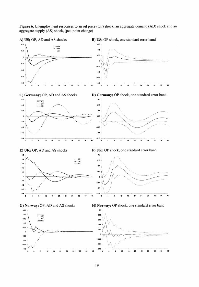
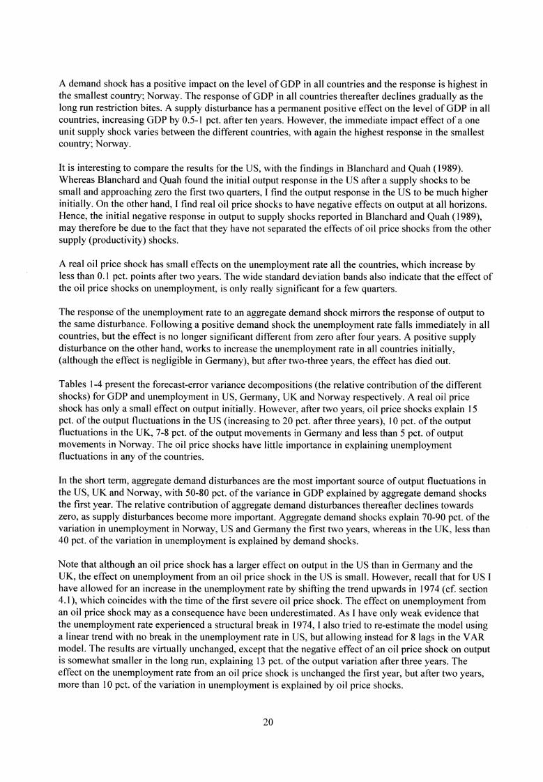
The cumulative dynamic effects (calculated from equation 28) of demand, supply and oil price shocks onGDP are reported in figures 5A-H, whereas the dynamic effects of the same three disturbances onunemployment are seen in figures 6A-H. In each figure, the dynamic effect of the oil price shock isreported with a standard deviation band around the point estimate. 12

In Germany, United Kingdom and United States, an adverse oil price shock (increase in the real price ofoil) lowers GDP the first two to three years. The effect is largest after six quarters, where the (onestandard error) oil price shock reduces GDP by 0.3-0.5 pct. The effect thereafter essentially dies out inGermany and UK, whereas for US, real GDP is permanently reduced with 0.4 pct. In Norway, theadverse oil price shock has an initial (negligible) negative effect on GDP, but the effect thereafterbecomes positive, and GDP has increased by about 0.4 pct. after two years. However, as the one standarderror band includes zero and becomes wider as the horizon increases, the effect may not be significant inthe long run.

12 The standard errors are calculated using Monte Carlo simulation based on normal random drawings from the distribution of thereduced form VAR. The draws are made directly from the posterior distribution of the VAR coefficients, as suggested in Doan(1992). The standard errors that correspond to the distributions in the D(L) matrix are then calculated using the estimate of Do .Impulse responses for all shocks with a standard deviation band, can be obtained from the author on request.

17

A) US; OP, AD and AS shocks B) US; OP shock, one standard error bando -

12 16 20 24 28 32 36 40 0 4 8 12 16 20 24 28 32 36 40

- ms-AS

0.2 -

0.8

0.6 -r

0.4 -0.

02 - -02 -

, - - OP ,

-AS 0.1

Figure 5. GDP impulse responses to an oil price (OP) shock, an aggregate demand (AD) shock and anaggregate supply (AS) shock, (pct. change)

C) Germany; OP, AD and AS shocks D) Germany; OP shock, one standard error band

0"'"" •

-0.3 -

-0.2

-0.4 -0.5

-- , . *%, -0.4 4

s

0 4 8 12 16 20 24 28 32 36 40 0 4 8 12 16 20 24 28 32 36 40

E) UK; OP, AD and AS shocks F) UK; OP shock, one standard error band12

1

0.8

0.6

0.4 -02

0.2 -

'.......... . . -0.4 --'0 - -___, ......•-' ...... . .... ------•........,,, . ‘

-0.5`,. / ‘ _ - . _ _ -

-- - - - - - -... - .... ...... --02 • , " '',. : .:"" ...--. ... ' •-• .-r-, - -0.6 --'- ..--...../.."*/\ / " -". ' - -- -

-0.4 - ...... ,"`4

„....,

-0.6 -0.8 0 4 8 12 16 20 24 28 32 36 40 0 4 8 12 16 20 24 28 32 36 40

G) Norway; OP, AD and AS shocks H) Norway; OP shock, one standard error band

, •-• .........

0.8 ,

uuf

02 -

•.

. ,• •

-0.4 -- .. . .. . .. . .

-0.2 -0.60 4 8 12 16 20 24 28 32 36 40 0 4 8 12 16 20 24 28 32 36 40

0.3

- OP 02-AS 0.1

0

-0.1

..........................

•• • ........................... .

0.4

0.2 -

o'-

o • .

l0

B) US; OP shock, one standard error bandA) US; OP, AD and AS shocks0.15 -

0.1 -

-0.2•

-0.3 -

-. s.

0.3 - 0.2 -

F) UK; OP shock, one standard error bandE) UK; OP, AD and AS shocks

-0.4 'O 4 8 12 16 20 24 28 32 36 40 0 4 8 12 16 20 24 28 32 36 40

0.2 -L

0.15 -

0.1 -;-•

O 4 8 12 16 20 24 28 32 36 40

-AS

0.1 7

4 8 12 16 20 24 28 32 36 40

G) Norway; OP, AD and AS shocks0.25 7-•

0.2

H) Norway; OP shock, one standard error band0.1 -

-0.2 -L

-0.3 L

0.06

Figure 6. Unemployment responses to an oil price (OP) shock, an aggregate demand (AD) shock and anaggregate supply (AS) shock, (pct. point change)

-0.4 -02O 4 8 12 16 20 24 28 32 36 40 0 4 8 12 16 20 24 28 32 36 40

C) Germany; OP, AD and AS shocks D) Germany; OP shock, one standard error band

0.05...... • -

0

-0.05

-0.1 T -0.02 -

-0.15 -0.04 -

-02 0 4 8 12 16 20 24 28 32 36 40 0 4 8 12 16 20 24 28 32 36 40

......

19

A demand shock has a positive impact on the level of GDP in all countries and the response is highest inthe smallest country; Norway. The response of GDP in all countries thereafter declines gradually as thelong run restriction bites. A supply disturbance has a permanent positive effect on the level of GDP in allcountries, increasing GDP by 0.5-1 pct. after ten years. However, the immediate impact effect of a oneunit supply shock varies between the different countries, with again the highest response in the smallestcountry; Norway.

It is interesting to compare the results for the US, with the findings in Blanchard and Quah (1989).Whereas Blanchard and Quah found the initial output response in the US after a supply shocks to besmall and approaching zero the first two quarters, I find the output response in the US to be much higherinitially. On the other hand, I find real oil price shocks to have negative effects on output at all horizons.Hence, the initial negative response in output to supply shocks reported in Blanchard and Quah (1989),may therefore be due to the fact that they have not separated the effects of oil price shocks from the othersupply (productivity) shocks.

A real oil price shock has small effects on the unemployment rate all the countries, which increase byless than 0.1 pct. points after two years. The wide standard deviation bands also indicate that the effect ofthe oil price shocks on unemployment, is only really significant for a few quarters.

The response of the unemployment rate to an aggregate demand shock mirrors the response of output tothe same disturbance. Following a positive demand shock the unemployment rate falls immediately in allcountries, but the effect is no longer significant different from zero after four years. A positive supplydisturbance on the other hand, works to increase the unemployment rate in all countries initially,(although the effect is negligible in Germany), but after two-three years, the effect has died out.

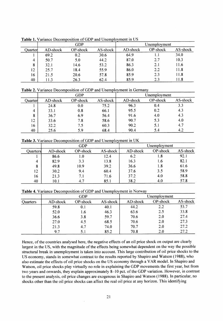
Tables 1-4 present the forecast-error variance decompositions (the relative contribution of the differentshocks) for GDP and unemployment in US, Germany, UK and Norway respectively. A real oil priceshock has only a small effect on output initially. However, after two years, oil price shocks explain 15pct. of the output fluctuations in the US (increasing to 20 pct. after three years), 10 pct. of the outputfluctuations in the UK, 7-8 pct. of the output movements in Germany and less than 5 pct. of outputmovements in Norway. The oil price shocks have little importance in explaining unemploymentfluctuations in any of the countries.

In the short term, aggregate demand disturbances are the most important source of output fluctuations inthe US, UK and Norway, with 50-80 pct. of the variance in GDP explained by aggregate demand shocksthe first year. The relative contribution of aggregate demand disturbances thereafter declines towardszero, as supply disturbances become more important. Aggregate demand shocks explain 70-90 pct. of thevariation in unemployment in Norway, US and Germany the first two years, whereas in the UK, less than40 pct. of the variation in unemployment is explained by demand shocks.

Note that although an oil price shock has a larger effect on output in the US than in Germany and theUK, the effect on unemployment from an oil price shock in the US is small. However, recall that for US Ihave allowed for an increase in the unemployment rate by shifting the trend upwards in 1974 (cf. section4.1), which coincides with the time of the first severe oil price shock. The effect on unemployment froman oil price shock may as a consequence have been underestimated. As I have only weak evidence thatthe unemployment rate experienced a structural break in 1974, I also tried to re-estimate the model usinga linear trend with no break in the unemployment rate in US, but allowing instead for 8 lags in the VARmodel. The results are virtually unchanged, except that the negative effect of an oil price shock on outputis somewhat smaller in the long run, explaining 13 pct. of the output variation after three years. Theeffect on the unemployment rate from an oil price shock is unchanged the first year, but after two years,more than 10 pct. of the variation in unemployment is explained by oil price shocks.

20

GDP Unemployment AD-shock OP-shock AS-shock

69.2

0.2

30.6

50.7

5.0

44.2

32.1

14.6

53.2

25.7

18.4

55.9

21.5

20.6

57.8

11.3

26.3

62.4

AD-shock OP-shock AS-shock

64.9 1.1 34.0

87.0 2.7 10.3

86.3 2.1 11.6

86.0 2.2 11.8

85.9 2.3 11.8

85.9 2.3 11.8

Quarte148

121640

r

GDP Unemployment AD-shock OP-shock AS-shock

24.8

0.0

75.2

33.1

0.8

66.1

36.7

6.9

56.4

33.6

7.8

58.6

32.2

7.5

60.3

25.6

5.9

68.4

AD-shock OP-shock AS-shock

96.3 0.4 3.3

95.5 0.2 4.3

91.6 4.0 4.3

90.7 5.3 4.0

90.2 5.1 4.7

90.4 5.4 4.2

Quarte148

121640

r

GDP Unemployment Quarter

148

121640

AD-shock86.682.949.830.221.310.1

OP-shock AS-shock

1.0

12.4

3.3

13.8

10.9

39.2

9.4

60.4

7.1

71.6

4.7

85.1

AD-shock OP-shock AS-shock

6.2 1.8 92.1

16.3 1.6 82.1

36.6 1.8 61.6

37.6 3.5 58.9

37.2 4.0 58.8

38.2 4.0 57.8

GDP Unemployment AD-shock OP-shock AS-shock

59.8

0.1

40.1

52.0

1.6

46.3

36.6

3.8

59.7

27.0

4.5

68.5

21.3

4.7

74.0

9.7

5.1

85.2

AD-shock OP-shock AS-shock

44.2 2.2 53.7

63.6 2.5 33.8

70.6 2.0 27.4

70.6 2.0 27.3

70.7 2.0 27.2

70.8 2.0 27.2

Quarters

Table 1. Variance Decomposition of GDP and Unemployment in US

Table 2. Variance Decomposition of GDP and Unem ploy ment in Germany

Table 3. Variance Decomposition of GDP and Unemployment in UK

Table 4. Variance Decom p osition of GDP and Unem ployment in Norway

Hence, of the countries analysed here, the negative effects of an oil price shock on output are clearlylargest in the US, with the magnitude of the effects being somewhat dependent on the way the possiblestructural break in unemployment is taken into account. This large contribution of oil price shocks to theUS economy, stands in somewhat contrast to the results reported by Shapiro and Watson (1988), whoalso estimate the effects of oil price shocks on the US economy through a VAR model. In Shapiro andWatson, oil price shocks play virtually no role in explaining the GDP movements the first year, but fromtwo years and onwards, they explain approximately 8-10 pct. of the GDP variation. However, in contrastto the present analysis, oil price changes are exogenous in Shapiro and Watson (1988). In particular, noshocks other than the oil price shocks can affect the real oil price at any horizon. This identifying

21

restrictions may in fact imply that Shapiro and Watson have underestimated the effects of oil priceshocks, and emphasised instead other supply shocks which may have similar effects on the variables inthe model (see also the comments made by Quah to their paper in the same journal).

To conclude then, why should output in the US respond more negatively to an oil price shock than outputin Germany (and UK), and why do Norway and UK (both being oil exporting countries) respond sodifferently?

The structure of the economy will probably play an important role for the macroeconomic adjustments tooil price shocks. Countries with low production dependence of oil, low share of oil in the consumptionbundle and relatively low labour intensities in production, will suffer less from oil price shocks. Germanyhas typically had a relatively small value of labour intensity in the traded goods sector and a low share ofoil in consumption, and may therefore have been less severely affected by the oil price increases, (seee.g. Lehment 1982, Fieleke 1988 and Nandakumar 1988). Rasche and Tatom (1981) suggest that asGermany has traditionally had higher duty on oil prices than US, it may therefore have replaced oil as anenergy source in some of the industry with nuclear power or coal. Especially, between 1973 and 1979,consumption of crude petroleum per capita declined slightly in Germany, whereas in the US it increased.Total import of crude petroleum also declined slightly between 1973 and 1979 in Germany, but increasedin the US, (cf. UN Yearbook of World Energy Statistics).

The fact that in the UK output decreased, whereas in Norway, output actually increased in response to anoil price shock, emphasises how two countries that are self sufficient with oil resources can react verydifferently to oil price shocks. Although the oil sector plays a much larger role in Norway than in the UK,macroeconomic policy has also been conducted very differently in light of the two major oil price shocksin Norway and the UK. In Norway, the oil price increases raised the net national wealth, allowing thegovernment to follow an expansionary fiscal policy during several periods. UK was self sufficient withoil resources when the second oil price shock occurred, but fiscal and monetary policies have remainedrelative tight during the 1980s, aimed primarily at combating the high inflation rates in that period. Withfactory closures and rapidly increasing unemployment rates from the late 1970s in the UK, much of therevenues from the increased oil prices instead went into social security in addition to payment of existingexternal debts.

Finally, the behaviour of output and unemployment in US, UK and Norway, seem consistent with what aKeynesian approach to business cycles would have predicted; Demand disturbances are the mostimportant factor behind output fluctuations in the short run, but eventually prices and wages adjust torestore equilibrium. In Germany, supply disturbances are more important than demand disturbances inexplaining output fluctuations in the short term, suggesting that a real business cycle view may beapplicable.

4.5. Sources of business cycles

Below I focus on specific historical periods by computing the forecast errors in output. The results arepresented in figures 7 for Norway 13 . In panels A-B, I plot the total forecast error in output together withthe forecast error that is due to oil price shocks and demand shocks respectively. In panel C, log GDP isgraphed together with the forecast error in output that is associated with the supply shock when the driftterm in the model is added (I will refer to this as the supply potential). The figure allows me to examinewhether the shocks identified can be well interpreted and assessed in terms of actual episodes thatoccurred in the periods examined.

In section 4.4, adverse oil price shocks were found to have positive effects on output in Norway. This isunderstood more clearly by examining figure 7A. The first oil price shock in 1973/1974 occurred at a

13 See Bjornland (2000b) for the results of the other three countries.

22

10- 143 7142 t

141

14 4

13.9*

13.8

137

las

8 T ...TOTAL;-AD

-2 -

-4 -

-8 70.3 733

-8 703 733 763 793 e23 85:3 833 913 943 763 793 823 E63 863 913 943763 793 823 E63 en 913 943 703 733

time when the Norwegian economy had just discovered huge oil resources in the North Sea. However,the prospect of increased oil revenues brought about by higher oil prices created a potential for profitableoutput. By the end of the 1970's, Norway was a net exporter of oil, so when the second oil price riseoccurred in 1979/1980, overall national wealth and demand increased further. Demand shocks were alsoimportant contributors behind the good economic performance in the middle 1970s, as the governmentfollowed expansionary fiscal policies from 1974-1977 (see figure 7B).

Figure 7. Forecast Error Decompositions for GDP in Norway

A) Oil price, B) Aggregate demand, C) Aggregate supply,(pct. change)

(pct. change)

(drift term added)

During the 1980s, Norway experienced two severe recessions. The first, from 1982 to 1985, wasprimarily demand driven. The economy thereafter experienced a demand driven boom, set off primarilyby a financial deregulation. The high growth rates were dampened somewhat by the collapse of oil pricesin 1986, which eroded the government of potential future income streams. From 1988, negative supplyshocks pushed the economy into another recession, and now both the supply potential and theunemployment rate changed permanently, (c.f. figure 7C and the discussion in section 4.3). The economyrecovered somewhat by 1990, but then the international economy was slowing down, and demand shockscontributed negatively to output growth.

4.6. Conclusions

By using a minimum of restrictions on a VAR model, I have been able to interpret economic fluctuationsin Germany, Norway, United Kingdom and United States in terms of three different shocks that have hitthe economy; Aggregate demand, aggregate supply and oil price shocks. In all countries, the dynamicadjustments of the variables are consistent with the economic model predictions, and the shocksidentified fit well with the actual events that have occurred in the different historical periods.

For all countries except Norway, an adverse oil price shock has had a negative effect on output in theshort run, and for the US, the effect is negative also in the long run (ten years). In Norway, (whose oilproducing sector plays a large role in the economy), the effect of oil price shocks on output is positive atall horizons, although in the long run the effect is not necessarily significant. The different responses inthe UK and Norway to an energy price shock, emphasise how two countries that are self sufficient withoil resources can react very differently to oil price shocks, especially if the governments have differentpriorities when deciding on macroeconomic policies.

Demand disturbances (temporary shocks) are the most important factors driving output in the short run inUnited States, United Kingdom and Norway, although already after two to three years (at the so calledbusiness cycle frequencies), supply shocks (permanent shocks) dominate. In Germany, supply shocksplay the most important role for output movements at all horizons.

23

Appendix A: Data sourcesAll series are seasonally adjusted quarterly data, unless otherwise stated. The series are seasonallyadjusted by their respective sources. The periodicity varies and is given for each country. All variablesare measured in natural logarithms except for the unemployment rate that is measured in levels. For eachcountry I use total GDP or GNP, except for Norway, where I use non-oil GDP, which accounts forapproximately 80 pct. of total GDP.

All countries:Nominal Oil price: Saudi Arabian Light-34, USD per barrel, fob- (n.s.a.). Prior to 1980, posted prices,thereafter spot prices. Source: OPEC BULLETIN and Statistics Norway

Real Oil Price: Nominal Oil Price converted to each countries national currency and deflated by eachcountries implicit GDP deflator, except for Norway which uses the consumer price index (as oil pricesmay be included in the GDP deflator, with approximately 20 pct. of GDP in Norway generated in the oilsector).

United States: 1960Q1-1994Q4Gross Domestic Product, constant 1991 prices. Source: OECDUnemployment, civil labour force. Source: OECDImplicit GDP deflator. Source: OECD

Germany: 1969Q1-1994Q4Gross Domestic Product, constant 1991 prices. Source: OECDUnemployment, (West Germany) . Source: OECDImplicit GDP deflator. Source: OECDExchange rate, mth. average DEM/USD, (n.s.a.). Source OECD.

United Kingdom: 1966Q1-1994Q4Gross Domestic Product, constant 1991 prices. Source: DatastreamUnemployment rate, total labour force. Source: OECDImplicit GDP deflator. Source: OECDExchange rate, mth. average GBF'/USD, (n.s.a.). Source OECD.

Norway: 1967Q1-1994Q4Gross Domestic Product, mainland Norway (GDP less petroleum activitiesand ocean transport) constant 1991 prices. Source: Statistics NorwayUnemployment rate. Source: Statistics NorwayConsumer Price Index. Source: Statistics NorwayExchange rate, mth. avg. NOK/USD, (n.s.a.). Source OECD.

24

ReferencesAhmed, E., J.B. Rosser and R.G. Sheehan (1988): A Global Model of OECD Aggregate Supply andDemand using Vector Autoregressive Techniques, European Economic Review, 32, 1711-1729.

Balke, N.S. and T.B. Fomby (1994): Large Shocks, Small Shocks, and Economic Fluctuations: Outliersin Macroeconomic Time Series, Journal of Applied Econometrics, 9, 181-200.

Banerjee, A., R.L. Lumsdaine and J.H. Stock (1992): Recursive and Sequential Tests of the Unit-Rootand Trend-Break Hypotheses: Theory and International Evidence, Journal of Business and EconomicStatistics, 10, 271-287.

Bayoumi, T. and B. Eichengreen (1992): Shocking Aspects of European Monetary Unification, CEPRDiscussion Paper no. 643.

Bernanke, B.S. (1986): Alternative explanations of the Money-Income Correlation, Carnegie-RochesterConference Series on Public Policy, 25, 49-99.

Beveridge, S. and C.R. Nelson (1981): A New Approach to the Decomposition of Economic Time Seriesinto Permanent and Transitory Components with Particular Attention to Meassurement of the 'BusinessCycle', Journal of Monetary Economics, 7, 151-174.

BjØrnland, H.C. (1998): The Economic Effects of North Sea Oil on the Manufacturing Sector, ScottishJournal of Political Economy, 45, pp. 553-585.

BjØrnland, H.C. (2000a): Detrending Methods and Stylized Facts of Business Cycles in Norway - Aninternational comparison, Empirical Economics, 25, 369-392.

BjØrnland, H.C. (2000b): The Dynamic Effects of Aggregate Demand, Supply and Oil Price Shocks - Acomparative study, The Manchester School of Economic Studies. Forthcoming.

Blanchard, O.J. (1989): A Traditional Interpretation of Macroeconomic Fluctuations, AmericanEconomic Review, 79, 1146-1164.

Blanchard, O.J and D. Quah (1989): The Dynamic Effects of Aggregate Demand and SupplyDisturbances, American Economic Review, 79, 655-673.

Blanchard, O.J and D. Quah (1993): Fundamentalness and the interpretation of time series evidence:Reply to Lippi and Reichlin, American Economic Review, 83, 653-658.

Blanchard, O.J and M.W. Watson (1986): "Are Business Cycles All Alike?", in R. Gordon, (ed.): TheAmerican Business cycle: Continuity and Change, NBER and University of Chicago Press, 123-56.

Bohi, D.R. (1989): Energy price shocks and macroeconomic performance, Washington: Resources forthe Future.

Brock, W.A. and C.L. Seyers (1988): Is the Business Cycle Characterised by Deterministic Chaos?,Journal of Monetary Economics, 22, 71-90.

Burbidge, J. and A. Harrison (1984): Testing for the Effects of Oil-Price Rises Using VectorAutoregressions, International Economic Review, 25, 459-484.

25

Canova, F. (1995a): "Vector Autoregressive Models: Specification, Estimation, Inference, andForecasting" in M.H. Pesaran and M. R. Wickens (eds.): Handbook of Applied Econometrics-Macroeconomics, Oxford: Blackwell Publishers. Ltd., 73-138.

Canova, F. (1995b): "The Economics of VAR Models", in K. Hoover (ed.): Macroeconometrics:Developments, Tensions and Prospects, Dortrecht: Kluwer Press, 57-97.

Clements, M.P. and G.E. Mizon (1991): Empirical analysis of macroeconomic time series. VAR andstructural models, European Economic Review, 35, 887-932.

Cooley, T. and S.F. LeRoy (1985): Atheoretical Macroeconomics. A Critique, Journal of MonetaryEconomics, 16, 283-308.

Darby, M. (1982): The Price of Oil and World Inflation and Recession, American Economic Review, 72,738-751

Doan, T.A. (1992): RATS User's Manual, Version 4, Estima.

Doornik, J.A. and D.F. Hendry (1994): PcFiml 8.0. Interactive Econometric Modelling of DynamicSystems, London: International Thomson Publishing.

Ericsson, N.R., D.F. Hendry and G.E. Mizon (1997): Econometric Issues in Economic Policy Analysis,manuscript, October 1997.

Faust, J. and E.M. Leeper (1997): When Do Long-Run Identifying Restrictions Give Reliable Results?,Journal of Business and Economic Statistics, 15, 345-353.

Fieleke, N.S. (1990): Oil Shock III?, New England Economic Review, September/October, 3-10.

Fischer, S. (1977): Long-Term Contracts, rational Expectations, and the Optimal Money Supply Rule,Journal of Political Economy, 85, 191-205.

Fuller, W. A. (1976): Introduction to Statistical Time Series, New York: Wiley.

Gali, J. (1992): How Well does the IS-LM Model fit Postwar U.S. Data?, Quarterly Journal ofEconomics, 107, 709-738.

Gisser, M. and T.H. Goodwin (1986): Crude Oil and the Macroeconomy: Test of Some Popular Notions,Journal of Money, Credit and Banking, 18, 95-103.

Hamilton, J.D. (1983): Oil and the Macroeconomy since World War II, Journal of Political Economy,91, 228-248.

Hendry, D.F. (1995): Econometrics and Business Cycle Empirics, The Economic Journal, 105, 1622-1636.

Hendry, D.F. and J.A. Doornik (1997): The Implications for Econometric Modelling of Forecast Failure,Scottish Journal of Political Economy, 44, 437-461.

Hendry, D.F. and G.E. Mizon (1991): "Evaluating Dynamic Econometric Models by Encompassing theVAR". In P.C.B. Phillips and V.B. Hall, (eds.), Models, Methods and Applications of Econometrics,Essays in the Honour of Rex Bergstrom, Oxford: Oxford University Press, 272-300.

26

Haavelmo, T. (1944): The Probability Approach in Economics, Econometrica, 12, (Supplement), 1-118.

James, J.A. (1993): Changes in Economic Instability in 19th-Century America, American EconomicReview, 83, 710-731.

Jevons, W.S. (1865): The Coal Question, London: Macmillian.

Johansen, S. (1988): Statistical Analysis of Cointegrating Vectors, Journal of Economic Dynamics andControl, 12, 231-254.

Johansen, S. (1991): Estimation and Hypothesis Testing of Cointegration Vectors in Gaussian VectorAutoregressive Models, Econometrica, 59, 1551-1580.

Keating, J.W. (1996): Structural information in recursive VAR orderings, Journal of EconomicDynamics and Control, 20, 1557-1580.

Kydland, F.E. and E.0 Prescott (1982): Time To Build and Aggregate Fluctuations, Econometrica, 50,1345-1370.

Layard, R., S. Nickel and R. Jackman (1991): Unemployment: Macroeconomic Performance and theLabour Market, Oxford University Press.

Lehment, H. (1982): Economic Policy Response to the Oil Price Shocks of 1974 and 1979, EuropeanEconomic Review, 18, 235-242.

Lippi, M. and L. Reichlin (1993): A note on measuring the dynamic effects of aggregate demand andaggregate supply disturbances, American Economic Review, 83, 644-652.

Liu, T.C. (1960): Underidentification, Structural Estimation, and Forecasting, Econometrica, 28, 855-865.

Lucas, R.E. Jr. (1976): "Econometric policy evaluation: a critique" in K. Brunner and A. Meltzer (eds.):The Phillips Curve and the Labor Market, Vol. 1 of Carnegie-Rochester Conference in Public Policy, asupplementation series to the Journal of Monetary Economics. Amsterdam: North Holland Publishers.

Liitkepohl, H. (1993): Introduction to Multiple Time Series Analysis, 2nd. ed., Berlin: Springer-Verlag.

Mork, K.A. (1994): Business Cycles and the Oil Market, Working Paper 1994/2, the Norwegian Schoolof Management.

Nandakumar, P. (1988): Oil Price Increases and the Structure of Small Open Economies,Weltwirtschaftliches Archiv, 124, 653-666.

Nelson, C.R. and C.I. Plosser (1982): Trends and Random Walks in Macroeconomic Time Series,Journal of Monetary Economics, 10, 129-162.

Osterwald-Lenum, M (1992): A Note with Quantiles of the Asymptotic Distribution of the MaximumLikelihood Cointegration Rank Test Statistics, Oxford Bulletin of Economics and Statistics, 54, 461-471.

Perron, P. (1989): The great Crash, the Oil Price Shock, and the Unit-root Hypothesis, Econometrica, 57,1361-1401.

27

Prescott, E. (1986): Theory Ahead of Business Cycle Measurement, Federal Reserve Bank ofMinneapolis Quarterly Review, 10, 9-22

Quah, D. T. (1992): The Relative Importance of permanent and Transitory Components: Identificationand Some Theoretical Bounds, Econometrica, 60, 107-118.

Rappoport, P. and L. Reichlin (1989): Segmented Trends and Non-Stationary Time Series, EconomicJournal, 99, Conference Supplement, 168-177.

Rasche, R.H. and J.A. Tatom (1981): Energy Price Shocks, Aggregate Supply and Monetary Policy: TheTheory and the International Evidence, Carnegie-Rochester Conference Series on Public Policy: SupplyShocks, Incentives and National Wealth, 14, 9-94.

Reimers, H.-E. (1992): Comparisons of tests for multivariate cointegration, Statistical Papers, 33, 335-359.

Sachs, J. (1982): The Oil Shocks and Macroeconomic adjustment in the United States, EuropeanEconomic Review, 18, 243-248.

Shapiro, M. and M.W. Watson (1988): "Sources of Business Cycle Fluctuations", in S. Fischer (ed.)Macroeconomics Annual, Cambridge: MIT Press, 111-148.

Sims, C.A. (1980): Macroeconomics and Reality, Econometrica, 48, 1-48.

Sims, C.A. (1986): Are Forecasting Models Useful for Policy Analysis?, Federal Reserve Bank ofMinneapolis Quarterly Review, Winter, 2-16.

Stock, J and M. Watson (1988): Testing for Common Trends, Journal of the American StatisticalAssociation, 83, 1097-1107.

West, K.D. (1988): On the Interpretation of Near Random-Walk Behaviour in GNP, The AmericanEconomic Review, 78, 202-209.1

Wickens, M.R. (1996): Interpreting cointegration vectors and common stochastic trends, Journal ofEconometrics, 74, 255-271.

Zarnowitz, V. (1991): What is a Business Cycle, NBER Working Paper No. 3863.

Zarnowitz, V. and G.H. Moore (1986): "Major Changes in Cyclical Behavior" in R.J. Gordon (ed.): TheAmerican Business Cycle, Chicago: The University of Chicago Press, 519-582.

Zivot, E and D.W. K. Andrews (1992): Further Evidence on the Great Crash, the Oil-Price Shock, andthe Unit-Root Hypothesis, Journal of Business and Economic Statistics, 10, 251-270.

28

Recent publications in the series Documents

99/3 K. Rypdal: Nomenclature for Solvent Produc-tion and Use

99/4 K. Rypdal and B. Tornsjo: Construction ofEnvironmental Pressure Information System(EPIS) for the Norwegian Offshore Oil and GasProduction

99/5 M. Soberg: Experimental Economics and theUS Tradable 502 Permit Scheme: A Discussionof Parallelism

99/6 J. Epland: Longitudinal non-response:Evidence from the Norwegian Income Panel

99/7 W. Yixuan and W. Taoyuan: The EnergyAccount in China: A Technical Documentation

99/8 T.L. Andersen and R. Johannessen: TheConsumer Price Index of Mozambique: A shortterm mission 29 November — 19 December1998

99/9 L-C. Zhang: SMAREST: A Survey of SMallARea ESTimation

99/10 L-C. Zhang: Some Norwegian Experience withSmall Area Estimation

99/11

H. Snorrason, 0. Ljones and B.K. Wold: Mid-Term Review: Twinning Arrangement 1997-2000, Palestinian Central Bureau of Statisticsand Statistics Norway, April 1999

99/12

K.-G. Lindquist: The Importance of Disaggre-gation in Economic Modelling

99/13

Y. Li: An Analysis of the Demand for SelectedDurables in China

99/14

T.I. Tysse and K. Vaage: Unemployment ofOlder Norwegian Workers: A Competing RiskAnalysis

1999/15 L. Solheim and D. Roll-Hansen: Photocopyingin Higher Education

1999/16 F. Brunvoll, E.H. Davila, V. Palm, S. Ribacke,K. Rypdal and L. Tangden: Inventory ofClimate Change Indicators for the NordicCountries.

1999/17 P. Schoning, M.V. Dysterud and E. Engelien:Computerised delimitation of urbansettlements: A method based on the use ofadministrative registers and digital maps.

1999/18 L.-C. Zhang and J. Sexton: ABC of Markovchain Monte Carlo

1999/19 K. Flugsrud, W. Irving and K. Rypdal:Methodological Choice in Inventory Prepara-tion. Suggestions for Good Practice Guidance

1999/20 K. Skrede: Gender Equality in the LabourMarket - still a Distant Goal?

1999/21 E. Engelien and P. Schoning: Land Use Statis-tics for Urban Settlements: Methods based onthe use of administrative registers and digitalmaps

1999/22 R. Kjeldstad: Lone Parents and the "WorkLine": Changing Welfare Schemes and Chang-ing Labour Market

2000/1 J.K. Dagsvik: Probabilistic Models forQualitative Choice Behavior: An Introduction

2000/2 A. Senhaji: "An Evaluation of someTechnology Programs executed by theNorwegian Government in the 80's and the 90's

2000/3 K. Rypdal and B. Tornsjo: EnvironmentalPressure Information System (EPIS) for thePulp and Paper Industry in Norway

2000/4 K. Rypdal and B. Toms* Chemicals inEnvironmental Pressure Information System(EPIS)

2000/5 R. Ragnarson: The Role of Subcontracting inthe Production System

2000/6 K.E. Rosendahl: Industrial Benefits and Costsof Greenhouse Gas Abatement Strategies:Applications of E3ME: Modelling externalsecondary benefits in the E3ME model

2000/7 G.A. Ellingsen, K.E. Rosendahl and A.Bruvoll: Industrial Benefits and Costs ofGreenhouse Gas Abatement Strategies:Applications of E3ME: Inclusion of 6greenhouse gases and other pollutants into theE3ME model

2000/8 R. Ragnarson and L. Solheim: IndustryStatistics in Mozambique: Major Findings andRecommendations

2000/9 R. Johannessen: The Consumer Price Index ofMozambique: A Short Term Mission 13-31March 2000

2000/10 B.K. Wold: Planned Co-operation withInstituto Nacional de Estatistica (INE),Mozambique: Report from Short TermIdentification Mission 27 th March to 3 rd April,2000 Requested by NORAD/Oslo

2000/11 P. Boug: Modelling Energy Demand inGermany: A Cointegration Approach

2000/12 E. Engelien and P. Scheming: Land usestatistics for urban settlements

2000/13 M. Ronsen: Impacts on Women's Work andChild Care Choices of Cash-for-Care Programs

29

Documents

E3 Returadresse:Statistisk sentralbyraN-2225 Kongsvinger

Statistics NorwayP.O.B. 8131 Dep.N-0033 Oslo

Tel: +47-22 86 45 00Fax: +47-22 86 49 73

ISSN 0805-9411

160 Statistisk sentralbythStatistics Norway