Embed Size (px)
Citation preview
Sage Primer for Linear Algebra
A First Course in Linear Algebra
Robert A. Beezer
University of Puget Sound
Version 3.11 (October 21, 2013)
c©20042013 Robert A. Beezer
Permission is granted to copy, distribute and/or modify this document under theterms of the GNU Free Documentation License, Version 1.2 or any later versionpublished by the Free Software Foundation; with no Invariant Sections, no Front-Cover Texts, and no Back-Cover Texts. A copy of the license is included in theappendix entitled “GNU Free Documentation License”.
Contents
Systems of Linear Equations 1Solving Systems of Linear Equations . . . . . . . . . . . . . . . . . . . . . 1Reduced Row-Echelon Form . . . . . . . . . . . . . . . . . . . . . . . . . . 5Types of Solution Sets . . . . . . . . . . . . . . . . . . . . . . . . . . . . . 12Homogeneous Systems of Equations . . . . . . . . . . . . . . . . . . . . . 16Nonsingular Matrices . . . . . . . . . . . . . . . . . . . . . . . . . . . . . . 18
Vectors 22Vector Operations . . . . . . . . . . . . . . . . . . . . . . . . . . . . . . . 22Linear Combinations . . . . . . . . . . . . . . . . . . . . . . . . . . . . . . 26Spanning Sets . . . . . . . . . . . . . . . . . . . . . . . . . . . . . . . . . . 30Linear Independence . . . . . . . . . . . . . . . . . . . . . . . . . . . . . . 37Linear Dependence and Spans . . . . . . . . . . . . . . . . . . . . . . . . . 40Orthogonality . . . . . . . . . . . . . . . . . . . . . . . . . . . . . . . . . . 44
Matrices 50Matrix Operations . . . . . . . . . . . . . . . . . . . . . . . . . . . . . . . 50Matrix Multiplication . . . . . . . . . . . . . . . . . . . . . . . . . . . . . 54Matrix Inverses and Systems of Linear Equations . . . . . . . . . . . . . . 57Matrix Inverses and Nonsingular Matrices . . . . . . . . . . . . . . . . . . 59Column and Row Spaces . . . . . . . . . . . . . . . . . . . . . . . . . . . . 62Four Subsets . . . . . . . . . . . . . . . . . . . . . . . . . . . . . . . . . . 68
Vector Spaces 73Subspaces . . . . . . . . . . . . . . . . . . . . . . . . . . . . . . . . . . . . 73Bases . . . . . . . . . . . . . . . . . . . . . . . . . . . . . . . . . . . . . . 74Dimension . . . . . . . . . . . . . . . . . . . . . . . . . . . . . . . . . . . . 78Properties of Dimension . . . . . . . . . . . . . . . . . . . . . . . . . . . . 80
Determinants 81Determinant of a Matrix . . . . . . . . . . . . . . . . . . . . . . . . . . . . 81Properties of Determinants of Matrices . . . . . . . . . . . . . . . . . . . . 84
Eigenvalues 87Eigenvalues and Eigenvectors . . . . . . . . . . . . . . . . . . . . . . . . . 87Properties of Eigenvalues and Eigenvectors . . . . . . . . . . . . . . . . . 92Similarity and Diagonalization . . . . . . . . . . . . . . . . . . . . . . . . 93
Linear Transformations 97Linear Transformations . . . . . . . . . . . . . . . . . . . . . . . . . . . . 97Injective Linear Transformations . . . . . . . . . . . . . . . . . . . . . . . 104Surjective Linear Transformations . . . . . . . . . . . . . . . . . . . . . . 107Invertible Linear Transformations . . . . . . . . . . . . . . . . . . . . . . . 110
Representations 115Vector Representations . . . . . . . . . . . . . . . . . . . . . . . . . . . . . 115Matrix Representations . . . . . . . . . . . . . . . . . . . . . . . . . . . . 117Change of Basis . . . . . . . . . . . . . . . . . . . . . . . . . . . . . . . . . 125
iii
Chapter SLESystems of Linear Equations
Section SSLE: Solving Systems of Linear Equations
GS Getting Started
Sage is a powerful system for studying and exploring many different areas of math-ematics. In the next section, and the majority of the remaining section, we willinslude short descriptions and examples using Sage. You can read a bit more aboutSage in the Preface. If you are not already reading this in an electronic version,you may want to investigate obtaining the worksheet version of this book, wherethe examples are “live” and editable. Most of your interaction with Sage will beby typing commands into a compute cell. That’s a compute cell just below thisparagraph. Click once inside the compute cell and you will get a more distinctiveborder around it, a blinking cursor inside, plus a cute little “evaluate” link belowit.
At the cursor, type 2+2 and then click on the evaluate link. Did a 4 appearbelow the cell? If so, you’ve successfully sent a command off for Sage to evaluateand you’ve received back the (correct) answer.
Here’s another compute cell. Try evaluating the command factorial(300).
Hmmmmm. That is quite a big integer! The slashes you see at the end of eachline mean the result is continued onto the next line, since there are 615 digits in theresult.
To make new compute cells, hover your mouse just above another compute cell,or just below some output from a compute cell. When you see a skinny blue baracross the width of your worksheet, click and you will open up a new computecell, ready for input. Note that your worksheet will remember any calculations youmake, in the order you make them, no matter where you put the cells, so it is bestto stay organized and add new cells at the bottom.
Try placing your cursor just below the monstrous value of 300! that you have.Click on the blue bar and try another factorial computation in the new computecell.
Each compute cell will show output due to only the very last command in thecell. Try to predict the following output before evaluating the cell.
1
Chapter SLE 2
a = 10
b = 6
a = a + 20
a
30
The following compute cell will not print anything since the one command doesnot create output. But it will have an effect, as you can see when you executethe subsequent cell. Notice how this uses the value of b from above. Execute thiscompute cell once. Exactly once. Even if it appears to do nothing. If you executethe cell twice, your credit card may be charged twice.
b = b + 50
Now execute this cell, which will produce some output.
b + 20
76
So b came into existence as 6. Then a cell added 50. This assumes you onlyexecuted this cell once! In the last cell we create b+20 (but do not save it) and it isthis value that is output.
You can combine several commands on one line with a semi-colon. This is a greatway to get multiple outputs from a compute cell. The syntax for building a ma-trix should be somewhat obvious when you see the output, but if not, it is notparticularly important to understand now.
f(x) = x^8 - 7*x^4; f
x |--> x^8 - 7*x^4
f; print ; f.derivative()
x |--> x^8 - 7*x^4
<BLANKLINE>
x |--> 8*x^7 - 28*x^3
g = f.derivative()
g.factor()
4*(2*x^4 - 7)*x^3
Some commands in Sage are “functions,” an example is factorial() above.Other commands are “methods” of an object and are like characteristics of objects,examples are .factor() and .derivative() as methods of a function. To com-ment on your work, you can open up a small word-processor. Hover your mouseuntil you get the skinny blue bar again, but now when you click, also hold theSHIFT key at the same time. Experiment with fonts, colors, bullet lists, etc andthen click the “Save changes” button to exit. Double-click on your text if you needto go back and edit it later.
Open the word-processor again to create a new bit of text (maybe next to the empty
Chapter SLE 3
compute cell just below). Type all of the following exactly, but do not include anybackslashes that might precede the dollar signs in the print version:
Pythagorean Theorem: \$c^2=a^2+b^2\$
and save your changes. The symbols between the dollar signs are written accord-ing to the mathematical typesetting language known as TeX — cruise the internetto learn more about this very popular tool. (Well, it is extremely popular amongmathematicians and physical scientists.)
Much of our interaction with sets will be through Sage lists. These are not reallysets — they allow duplicates, and order matters. But they are so close to sets, andso easy and powerful to use that we will use them regularly. We will use a funmade-up list for practice, the quote marks mean the items are just text, with nospecial mathematical meaning. Execute these compute cells as we work throughthem.
zoo = [’snake’, ’parrot’, ’elephant’, ’baboon’, ’beetle’]
zoo
[’snake’, ’parrot’, ’elephant’, ’baboon’, ’beetle’]
So the square brackets define the boundaries of our list, commas separate items,and we can give the list a name. To work with just one element of the list, we usethe name and a pair of brackets with an index. Notice that lists have indices thatbegin counting at zero. This will seem odd at first and will seem very natural later.
zoo[2]
’elephant’
We can add a new creature to the zoo, it is joined up at the far right end.
zoo.append(’ostrich’); zoo
[’snake’, ’parrot’, ’elephant’, ’baboon’, ’beetle’, ’ostrich’]
We can remove a creature.
zoo.remove(’parrot’)
zoo
[’snake’, ’elephant’, ’baboon’, ’beetle’, ’ostrich’]
We can extract a sublist. Here we start with element 1 (the elephant) and goall the way up to, but not including, element 3 (the beetle). Again a bit odd, but itwill feel natural later. For now, notice that we are extracting two elements of thelists, exactly 3− 1 = 2 elements.
mammals = zoo[1:3]
mammals
[’elephant’, ’baboon’]
Chapter SLE 4
Often we will want to see if two lists are equal. To do that we will need to sorta list first. A function creates a new, sorted list, leaving the original alone. So weneed to save the new one with a new name.
newzoo = sorted(zoo)
newzoo
[’baboon’, ’beetle’, ’elephant’, ’ostrich’, ’snake’]
zoo.sort()
zoo
[’baboon’, ’beetle’, ’elephant’, ’ostrich’, ’snake’]
Notice that if you run this last compute cell your zoo has changed and somecommands above will not necessarily execute the same way. If you want to experi-ment, go all the way back to the first creation of the zoo and start executing cellsagain from there with a fresh zoo.
A construction called a “list comprehension” is especially powerful, especially sinceit almost exactly mirrors notation we use to describe sets. Suppose we want to formthe plural of the names of the creatures in our zoo. We build a new list, based onall of the elements of our old list.
plurality_zoo = [animal+’s’ for animal in zoo]
plurality_zoo
[’baboons’, ’beetles’, ’elephants’, ’ostrichs’, ’snakes’]
Almost like it says: we add an “s” to each animal name, for each animal inthe zoo, and place them in a new list. Perfect. (Except for getting the plural of“ostrich” wrong.)
One final type of list, with numbers this time. The range() function will cre-ate lists of integers. In its simplest form an invocation like range(12) will create alist of 12 integers, starting at zero and working up to, but not including, 12. Doesthis sound familiar?
dozen = range(12); dozen
[0, 1, 2, 3, 4, 5, 6, 7, 8, 9, 10, 11]
Here are two other forms, that you should be able to understand by studyingthe examples.
teens = range(13, 20); teens
[13, 14, 15, 16, 17, 18, 19]
decades = range(1900, 2000, 10); decades
[1900, 1910, 1920, 1930, 1940, 1950, 1960, 1970, 1980, 1990]
There is a “Save” button in the upper-right corner of your worksheet. Thiswill save a current copy of your worksheet that you can retrieve from within your
Chapter SLE 5
notebook again later, though you have to re-execute all the cells when you re-openthe worksheet later.
There is also a “File” drop-down list, on the left, just above your very top computecell (not be confused with your browser’s File menu item!). You will see a choicehere labeled “Save worksheet to a file...” When you do this, you are creating acopy of your worksheet in the “sws” format (short for “Sage WorkSheet”). You canemail this file, or post it on a website, for other Sage users and they can use the“Upload” link on their main notebook page to incorporate a copy of your worksheetinto their notebook.
There are other ways to share worksheets that you can experiment with, but thisgives you one way to share any worksheet with anybody almost anywhere.
We have covered a lot here in this section, so come back later to pick up tidbitsyou might have missed. There are also many more features in the notebook thatwe have not covered.
Section RREF: Reduced Row-Echelon Form
M Matrices
Matrices are fundamental objects in linear algebra and in Sage, so there are a va-riety of ways to construct a matrix in Sage. Generally, you need to specify whattypes of entries the matrix contains (more on that in a minute), the number of rowsand columns, and the entries themselves. First, let’s dissect an example:
A = matrix(QQ, 2, 3, [[1, 2, 3], [4, 5, 6]])
A
[1 2 3]
[4 5 6]
QQ is the set of all rational numbers (fractions with an integer numerator anddenominator), 2 is the number of rows, 3 is the number of columns. Sage under-stands a list of items as delimited by brackets ([,]) and the items in the list canagain be lists themselves. So [[1, 2, 3], [4, 5, 6]] is a list of lists, and in thiscontext the inner lists are rows of the matrix.
There are various shortcuts you can employ when creating a matrix. For exam-ple, Sage is able to infer the size of the matrix from the lists of entries.
B = matrix(QQ, [[1, 2, 3], [4, 5, 6]])
B
[1 2 3]
[4 5 6]
Or you can specify how many rows the matrix will have and provide one biggrand list of entries, which will get chopped up, row by row, if you prefer.
C = matrix(QQ, 2, [1, 2, 3, 4, 5, 6])
C
[1 2 3]
[4 5 6]
Chapter SLE 6
It is possible to also skip specifying the type of numbers used for entries of a ma-trix, however this is fraught with peril, as Sage will make an informed guess aboutyour intent. Is this what you want? Consider when you enter the single character“2” into a computer program like Sage. Is this the integer 2, the rational number 2
1 ,the real number 2.00000, the complex number 2 + 0i, or the polynomial p(x) = 2?In context, us humans can usually figure it out, but a literal-minded computer isnot so smart. It happens that the operations we can perform, and how they behave,are influenced by the type of the entries in a matrix. So it is important to get thisright and our advice is to be explicit and be in the habit of always specifying thetype of the entries of a matrix you create.
Mathematical objects in Sage often come from sets of similar objects. This setis called the “parent” of the element. We can use this to learn how Sage deducesthe type of entries in a matrix. Execute the following three compute cells in theSage notebook, and notice how the three matrices are constructed to have entriesfrom the integers, the rationals and the reals.
A = matrix(2, 3, [[1, 2, 3], [4, 5, 6]])
A.parent()
Full MatrixSpace of 2 by 3 dense matrices over Integer Ring
B = matrix(2, 3, [[1, 2/3, 3], [4, 5, 6]])
B.parent()
Full MatrixSpace of 2 by 3 dense matrices over Rational Field
C = matrix(2, 3, [[1, sin(2.2), 3], [4, 5, 6]])
C.parent()
Full MatrixSpace of 2 by 3 dense matrices over
Real Field with 53 bits of precision
Sage knows a wide variety of sets of numbers. These are known as “rings” or“fields” (see Section F), but we will call them “number systems” here. Examplesinclude: ZZ is the integers, QQ is the rationals, RR is the real numbers with reason-able precision, and CC is the complex numbers with reasonable precision. We willpresent the theory of linear algebra over the complex numbers. However, in anycomputer system, there will always be complications surrounding the inability ofdigital arithmetic to accurately represent all complex numbers. In contrast, Sagecan represent rational numbers exactly as the quotient of two (perhaps very large)integers. So our Sage examples will begin by using QQ as our number system andwe can concentrate on understanding the key concepts.
Once we have constructed a matrix, we can learn a lot about it (such as its parent).Sage is largely object-oriented, which means many commands apply to an objectby using the “dot” notation. A.parent() is an example of this syntax, while theconstructor matrix([[1, 2, 3], [4, 5, 6]]) is an exception. Here are a fewexamples, followed by some explanation:
A = matrix(QQ, 2, 3, [[1,2,3],[4,5,6]])
A.nrows(), A.ncols()
(2, 3)
Chapter SLE 7
A.base_ring()
Rational Field
A[1,1]
5
A[1,2]
6
The number of rows and the number of columns should be apparent, .base_ring()gives the number system for the entries, as included in the information provided by.parent().
Computer scientists and computer languages prefer to begin counting from zero,while mathematicians and written mathematics prefer to begin counting at one.Sage and this text are no exception. It takes some getting used to, but the reasonsfor counting from zero in computer programs soon becomes very obvious. Countingfrom one in mathematics is historical, and unlikely to change anytime soon. Soabove, the two rows of A are numbered 0 and 1, while the columns are numbered 0,1 and 2. So A[1,2] refers to the entry of A in the second row and the third column,i.e. 6.
There is much more to say about how Sage works with matrices, but this is al-ready a lot to digest. Use the space below to create some matrices (different ways)and examine them and their properties (size, entries, number system, parent).
V Vectors
Vectors in Sage are built, manipulated and interrogated in much the same wayas matrices (see Sage M). However as simple lists (“one-dimensional,” not “two-dimensional” such as matrices that look more tabular) they are simpler to constructand manipulate. Sage will print a vector across the screen, even if we wish tointerpret it as a column vector. It will be delimited by parentheses ((,)) whichallows us to distinguish a vector from a matrix with just one row, if we look carefully.The number of “slots” in a vector is not referred to in Sage as rows or columns,but rather by “degree.” Here are some examples (remember to start counting fromzero):
v = vector(QQ, 4, [1, 1/2, 1/3, 1/4])
v
(1, 1/2, 1/3, 1/4)
v.degree()
4
v.parent()
Chapter SLE 8
Vector space of dimension 4 over Rational Field
v[2]
1/3
w = vector([1, 2, 3, 4, 5, 6])
w
(1, 2, 3, 4, 5, 6)
w.degree()
6
w.parent()
Ambient free module of rank 6 over
the principal ideal domain Integer Ring
w[3]
4
Notice that if you use commands like .parent() you will sometimes see refer-ences to “free modules.” This is a technical generalization of the notion of a vector,which is beyond the scope of this course, so just mentally convert to vectors whenyou see this term.
The zero vector is super easy to build, but be sure to specify what number sys-tem your zero is from.
z = zero_vector(QQ, 5)
z
(0, 0, 0, 0, 0)
Notice that while using Sage, we try to remain consistent with our mathematicalnotation conventions. This is not required, as you can give items in Sage very longnames if you wish. For example, the following is perfectly legitimate, as you cansee.
blatzo = matrix(QQ, 2, [1, 2, 3, 4])
blatzo
[1 2]
[3 4]
In fact, our use of capital letters for matrices actually contradicts some of theconventions for naming objects in Sage, so there are good reasons for not mirroringour mathematical notation.
Chapter SLE 9
AM Augmented Matrix
Sage has a matrix method, .augment(), that will join two matrices, side-by-sideprovided they both have the same number of rows. The same method will allow youto augment a matrix with a column vector, as described in Definition AM, providedthe number of entries in the vector matches the number of rows for the matrix. Herewe reprise the construction in Example AMAA. We will now format our matricesas input across several lines, a practice you may use in your own worksheets, or not.
A = matrix(QQ, 3, 3, [[1, -1, 2],
[2, 1, 1],
[1, 1, 0]])
b = vector(QQ, [1, 8, 5])
M = A.augment(b)
M
[ 1 -1 2 1]
[ 2 1 1 8]
[ 1 1 0 5]
Notice that the matrix method .augment() needs some input, in the above case,the vector b. This will explain the need for the parentheses on the end of the “dot”commands, even if the particular command does not expect input.
Some methods allow optional input, typically using keywords. Matrices can tracksubdivisions, making breaks between rows and/or columns. When augmenting, youcan ask for the subdivision to be included. Evalute the compute cell above if youhave not already, so that A and b are defined, and then evaluate:
M = A.augment(b, subdivide=True)
M
[ 1 -1 2| 1]
[ 2 1 1| 8]
[ 1 1 0| 5]
As a partial demonstration of manipulating subdivisions of matrices we can resetthe subdivisions of M with the .subdivide() method. We provide a list of rowsto subdivide before, then a list of columns to subdivide before, where we rememberthat counting begins at zero.
M.subdivide([1,2],[1])
M
[ 1|-1 2 1]
[--+--------]
[ 2| 1 1 8]
[--+--------]
[ 1| 1 0 5]
RO Row Operations
Sage will perform individual row operations on a matrix. This can get a bit tedious,but it is better than doing the computations (wrong, perhaps) by hand, and it canbe useful when building up more complicated procedures for a matrix.
For each row operation, there are two similar methods. One changes the matrix
Chapter SLE 10
“in-place” while the other creates a new matrix that is a modified version of theoriginal. This is an important distinction that you should understand for every newSage command you learn that might change a matrix or vector.
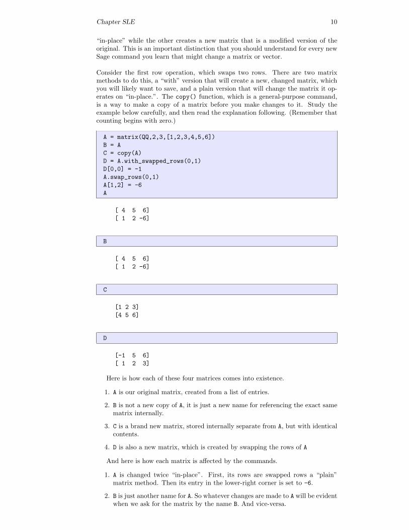
Consider the first row operation, which swaps two rows. There are two matrixmethods to do this, a “with” version that will create a new, changed matrix, whichyou will likely want to save, and a plain version that will change the matrix it op-erates on “in-place.”. The copy() function, which is a general-purpose command,is a way to make a copy of a matrix before you make changes to it. Study theexample below carefully, and then read the explanation following. (Remember thatcounting begins with zero.)
A = matrix(QQ,2,3,[1,2,3,4,5,6])
B = A
C = copy(A)
D = A.with_swapped_rows(0,1)
D[0,0] = -1
A.swap_rows(0,1)
A[1,2] = -6
A
[ 4 5 6]
[ 1 2 -6]
B
[ 4 5 6]
[ 1 2 -6]
C
[1 2 3]
[4 5 6]
D
[-1 5 6]
[ 1 2 3]
Here is how each of these four matrices comes into existence.
1. A is our original matrix, created from a list of entries.
2. B is not a new copy of A, it is just a new name for referencing the exact samematrix internally.
3. C is a brand new matrix, stored internally separate from A, but with identicalcontents.
4. D is also a new matrix, which is created by swapping the rows of A
And here is how each matrix is affected by the commands.
1. A is changed twice “in-place”. First, its rows are swapped rows a “plain”matrix method. Then its entry in the lower-right corner is set to -6.
2. B is just another name for A. So whatever changes are made to A will be evidentwhen we ask for the matrix by the name B. And vice-versa.
Chapter SLE 11
3. C is a copy of the original A and does not change, since no subsequent com-mands act on C.
4. D is a new copy of A, created by swapping the rows of A. Once created from A,it has a life of its own, as illustrated by the change in its entry in the upper-leftcorner to -1.
An interesting experiment is to rearrange some of the lines above (or add newones) and predict the result.
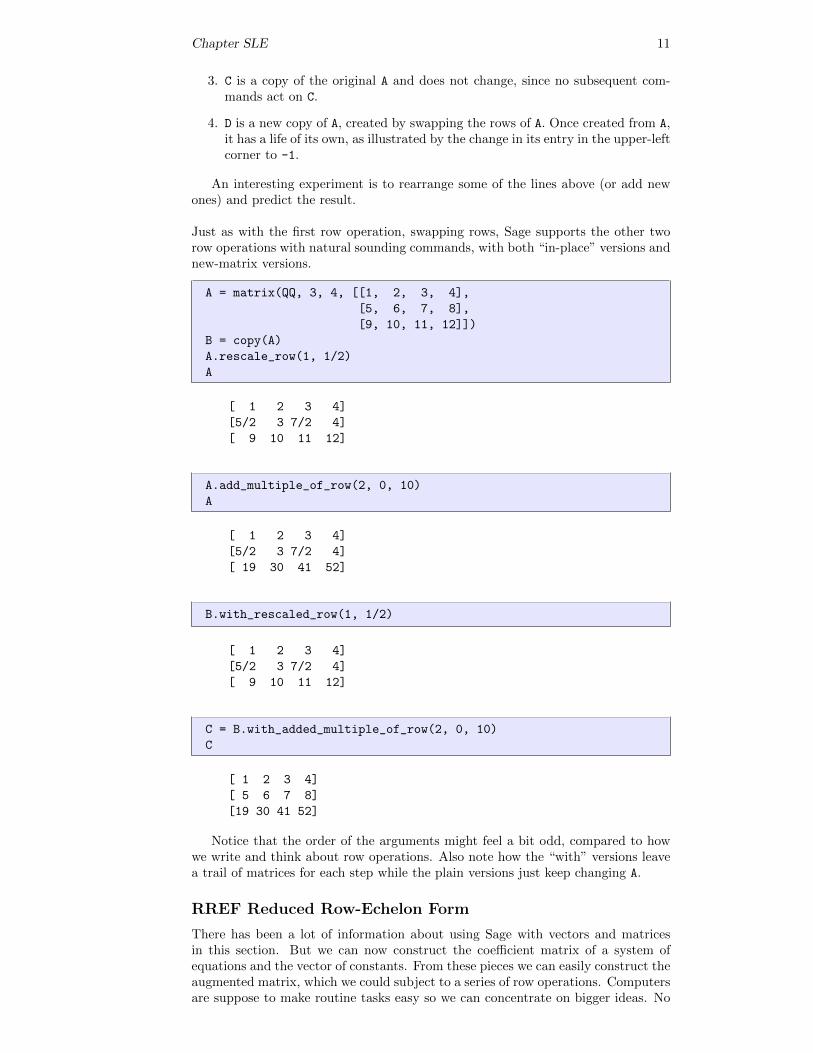
Just as with the first row operation, swapping rows, Sage supports the other tworow operations with natural sounding commands, with both “in-place” versions andnew-matrix versions.
A = matrix(QQ, 3, 4, [[1, 2, 3, 4],
[5, 6, 7, 8],
[9, 10, 11, 12]])
B = copy(A)
A.rescale_row(1, 1/2)
A
[ 1 2 3 4]
[5/2 3 7/2 4]
[ 9 10 11 12]
A.add_multiple_of_row(2, 0, 10)
A
[ 1 2 3 4]
[5/2 3 7/2 4]
[ 19 30 41 52]
B.with_rescaled_row(1, 1/2)
[ 1 2 3 4]
[5/2 3 7/2 4]
[ 9 10 11 12]
C = B.with_added_multiple_of_row(2, 0, 10)
C
[ 1 2 3 4]
[ 5 6 7 8]
[19 30 41 52]
Notice that the order of the arguments might feel a bit odd, compared to howwe write and think about row operations. Also note how the “with” versions leavea trail of matrices for each step while the plain versions just keep changing A.
RREF Reduced Row-Echelon Form
There has been a lot of information about using Sage with vectors and matricesin this section. But we can now construct the coefficient matrix of a system ofequations and the vector of constants. From these pieces we can easily construct theaugmented matrix, which we could subject to a series of row operations. Computersare suppose to make routine tasks easy so we can concentrate on bigger ideas. No
Chapter SLE 12
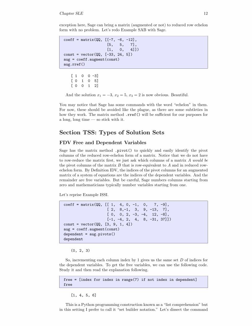
exception here, Sage can bring a matrix (augmented or not) to reduced row echelonform with no problem. Let’s redo Example SAB with Sage.
coeff = matrix(QQ, [[-7, -6, -12],
[5, 5, 7],
[1, 0, 4]])
const = vector(QQ, [-33, 24, 5])
aug = coeff.augment(const)
aug.rref()
[ 1 0 0 -3]
[ 0 1 0 5]
[ 0 0 1 2]
And the solution x1 = −3, x2 = 5, x3 = 2 is now obvious. Beautiful.
You may notice that Sage has some commands with the word “echelon” in them.For now, these should be avoided like the plague, as there are some subtleties inhow they work. The matrix method .rref() will be sufficient for our purposes fora long, long time — so stick with it.
Section TSS: Types of Solution Sets
FDV Free and Dependent Variables
Sage has the matrix method .pivot() to quickly and easily identify the pivotcolumns of the reduced row-echelon form of a matrix. Notice that we do not haveto row-reduce the matrix first, we just ask which columns of a matrix A would bethe pivot columns of the matrix B that is row-equivalent to A and in reduced row-echelon form. By Definition IDV, the indices of the pivot columns for an augmentedmatrix of a system of equations are the indices of the dependent variables. And theremainder are free variables. But be careful, Sage numbers columns starting fromzero and mathematicians typically number variables starting from one.
Let’s reprise Example ISSI.
coeff = matrix(QQ, [[ 1, 4, 0, -1, 0, 7, -9],
[ 2, 8,-1, 3, 9, -13, 7],
[ 0, 0, 2, -3, -4, 12, -8],
[-1, -4, 2, 4, 8, -31, 37]])
const = vector(QQ, [3, 9, 1, 4])
aug = coeff.augment(const)
dependent = aug.pivots()
dependent
(0, 2, 3)
So, incrementing each column index by 1 gives us the same set D of indices forthe dependent variables. To get the free variables, we can use the following code.Study it and then read the explanation following.
free = [index for index in range(7) if not index in dependent]
free
[1, 4, 5, 6]
This is a Python programming construction known as a “list comprehension” butin this setting I prefer to call it “set builder notation.” Let’s dissect the command
Chapter SLE 13
in pieces. The brackets ([,]) create a new list. The items in the list will be valuesof the variable index. range(7) is another list, integers starting at 0 and stoppingjust before 7. (While perhaps a bit odd, this works very well when we consistentlystart counting at zero.) So range(7) is the list [0,1,2,3,4,5,6]. Think of theseas candidate values for index, which are generated by for index in range(7).Then we test each candidate, and keep it in the new list if it is not in the listdependent.
This is entirely analogous to the following mathematics:
F = {f | 1 ≤ f ≤ 7, f 6∈ D}
where F is free, f is index, and D is dependent, and we make the 0/1 countingadjustments. This ability to construct sets in Sage with notation so closely mirroringthe mathematics is a powerful feature worth mastering. We will use it repeatedly.It was a good exercise to use a list comprehension to form the list of columns thatare not pivot columns. However, Sage has us covered.
free_and_easy = coeff.nonpivots()
free_and_easy
(1, 4, 5, 6)
Can you use this new matrix method to make a simpler version of the consistent()function we designed above?
RCLS Recognizing Consistency of a Linear System
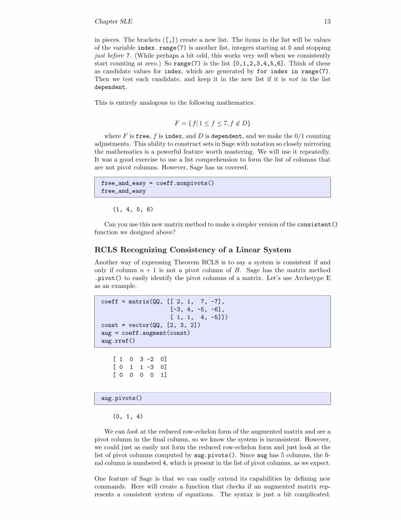
Another way of expressing Theorem RCLS is to say a system is consistent if andonly if column n + 1 is not a pivot column of B. Sage has the matrix method.pivot() to easily identify the pivot columns of a matrix. Let’s use Archetype Eas an example.
coeff = matrix(QQ, [[ 2, 1, 7, -7],
[-3, 4, -5, -6],
[ 1, 1, 4, -5]])
const = vector(QQ, [2, 3, 2])
aug = coeff.augment(const)
aug.rref()
[ 1 0 3 -2 0]
[ 0 1 1 -3 0]
[ 0 0 0 0 1]
aug.pivots()
(0, 1, 4)
We can look at the reduced row-echelon form of the augmented matrix and see apivot column in the final column, so we know the system is inconsistent. However,we could just as easily not form the reduced row-echelon form and just look at thelist of pivot columns computed by aug.pivots(). Since aug has 5 columns, the fi-nal column is numbered 4, which is present in the list of pivot columns, as we expect.
One feature of Sage is that we can easily extend its capabilities by defining newcommands. Here will create a function that checks if an augmented matrix rep-resents a consistent system of equations. The syntax is just a bit complicated.
Chapter SLE 14
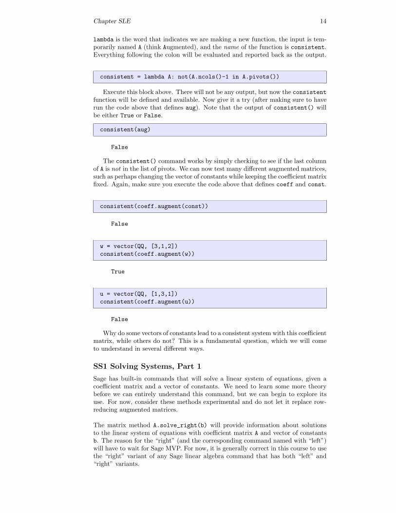
lambda is the word that indicates we are making a new function, the input is tem-porarily named A (think Augmented), and the name of the function is consistent.Everything following the colon will be evaluated and reported back as the output.
consistent = lambda A: not(A.ncols()-1 in A.pivots())
Execute this block above. There will not be any output, but now the consistentfunction will be defined and available. Now give it a try (after making sure to haverun the code above that defines aug). Note that the output of consistent() willbe either True or False.
consistent(aug)
False
The consistent() command works by simply checking to see if the last columnof A is not in the list of pivots. We can now test many different augmented matrices,such as perhaps changing the vector of constants while keeping the coefficient matrixfixed. Again, make sure you execute the code above that defines coeff and const.
consistent(coeff.augment(const))
False
w = vector(QQ, [3,1,2])
consistent(coeff.augment(w))
True
u = vector(QQ, [1,3,1])
consistent(coeff.augment(u))
False
Why do some vectors of constants lead to a consistent system with this coefficientmatrix, while others do not? This is a fundamental question, which we will cometo understand in several different ways.
SS1 Solving Systems, Part 1
Sage has built-in commands that will solve a linear system of equations, given acoefficient matrix and a vector of constants. We need to learn some more theorybefore we can entirely understand this command, but we can begin to explore itsuse. For now, consider these methods experimental and do not let it replace row-reducing augmented matrices.
The matrix method A.solve_right(b) will provide information about solutionsto the linear system of equations with coefficient matrix A and vector of constantsb. The reason for the “right” (and the corresponding command named with “left”)will have to wait for Sage MVP. For now, it is generally correct in this course to usethe “right” variant of any Sage linear algebra command that has both “left” and“right” variants.
Chapter SLE 15
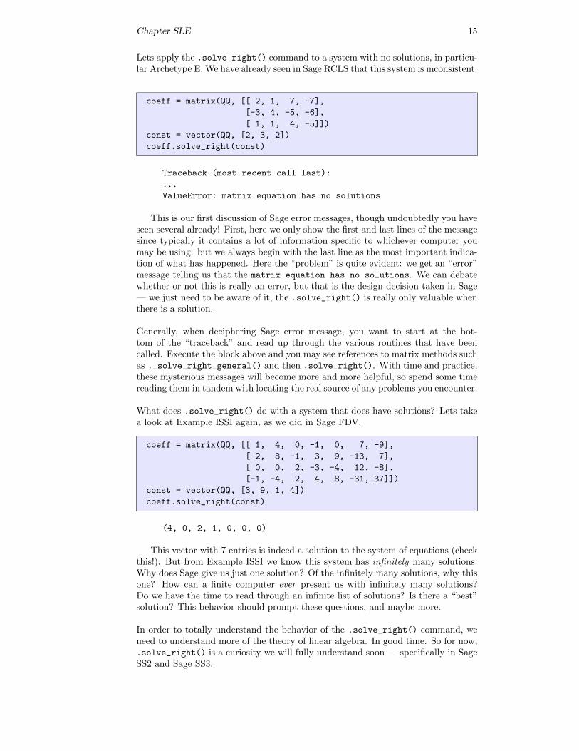
Lets apply the .solve_right() command to a system with no solutions, in particu-lar Archetype E. We have already seen in Sage RCLS that this system is inconsistent.
coeff = matrix(QQ, [[ 2, 1, 7, -7],
[-3, 4, -5, -6],
[ 1, 1, 4, -5]])
const = vector(QQ, [2, 3, 2])
coeff.solve_right(const)
Traceback (most recent call last):
...
ValueError: matrix equation has no solutions
This is our first discussion of Sage error messages, though undoubtedly you haveseen several already! First, here we only show the first and last lines of the messagesince typically it contains a lot of information specific to whichever computer youmay be using. but we always begin with the last line as the most important indica-tion of what has happened. Here the “problem” is quite evident: we get an “error”message telling us that the matrix equation has no solutions. We can debatewhether or not this is really an error, but that is the design decision taken in Sage— we just need to be aware of it, the .solve_right() is really only valuable whenthere is a solution.
Generally, when deciphering Sage error message, you want to start at the bot-tom of the “traceback” and read up through the various routines that have beencalled. Execute the block above and you may see references to matrix methods suchas ._solve_right_general() and then .solve_right(). With time and practice,these mysterious messages will become more and more helpful, so spend some timereading them in tandem with locating the real source of any problems you encounter.
What does .solve_right() do with a system that does have solutions? Lets takea look at Example ISSI again, as we did in Sage FDV.
coeff = matrix(QQ, [[ 1, 4, 0, -1, 0, 7, -9],
[ 2, 8, -1, 3, 9, -13, 7],
[ 0, 0, 2, -3, -4, 12, -8],
[-1, -4, 2, 4, 8, -31, 37]])
const = vector(QQ, [3, 9, 1, 4])
coeff.solve_right(const)
(4, 0, 2, 1, 0, 0, 0)
This vector with 7 entries is indeed a solution to the system of equations (checkthis!). But from Example ISSI we know this system has infinitely many solutions.Why does Sage give us just one solution? Of the infinitely many solutions, why thisone? How can a finite computer ever present us with infinitely many solutions?Do we have the time to read through an infinite list of solutions? Is there a “best”solution? This behavior should prompt these questions, and maybe more.
In order to totally understand the behavior of the .solve_right() command, weneed to understand more of the theory of linear algebra. In good time. So for now,.solve_right() is a curiosity we will fully understand soon — specifically in SageSS2 and Sage SS3.
Chapter SLE 16
Section HSE: Homogeneous Systems of Equations
SHS Solving Homogeneous Systems
We can explore homogeneous systems easily in Sage with commands we have alreadylearned. Notably, the zero_vector() constructor will quickly create the necessaryvector of constants (Sage V).
You could try defining a function to accept a matrix as input, augment the matrixwith a zero vector having the right number of entries, and then return the reducedrow-echelon form of the augmented matrix, or maybe you could return the numberof free variables. (See Sage RCLS for a refresher on how to do this). It is alsointeresting to see how .solve_right() behaves on homogeneous systems, since inparticular we know it will never give us an error. (Why not? Hint: Theorem HSC.)
NS Null Space
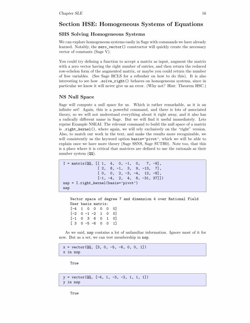
Sage will compute a null space for us. Which is rather remarkable, as it is aninfinite set! Again, this is a powerful command, and there is lots of associatedtheory, so we will not understand everything about it right away, and it also hasa radically different name in Sage. But we will find it useful immediately. Letsreprise Example NSEAI. The relevant command to build the null space of a matrixis .right_kernel(), where again, we will rely exclusively on the “right” version.Also, to match our work in the text, and make the results more recognizable, wewill consistently us the keyword option basis=’pivot’, which we will be able toexplain once we have more theory (Sage SSNS, Sage SUTH0). Note too, that thisis a place where it is critical that matrices are defined to use the rationals as theirnumber system (QQ).
I = matrix(QQ, [[ 1, 4, 0, -1, 0, 7, -9],
[ 2, 8, -1, 3, 9, -13, 7],
[ 0, 0, 2, -3, -4, 12, -8],
[-1, -4, 2, 4, 8, -31, 37]])
nsp = I.right_kernel(basis=’pivot’)
nsp
Vector space of degree 7 and dimension 4 over Rational Field
User basis matrix:
[-4 1 0 0 0 0 0]
[-2 0 -1 -2 1 0 0]
[-1 0 3 6 0 1 0]
[ 3 0 -5 -6 0 0 1]
As we said, nsp contains a lot of unfamiliar information. Ignore most of it fornow. But as a set, we can test membership in nsp.
x = vector(QQ, [3, 0, -5, -6, 0, 0, 1])
x in nsp
True
y = vector(QQ, [-4, 1, -3, -2, 1, 1, 1])
y in nsp
True
Chapter SLE 17
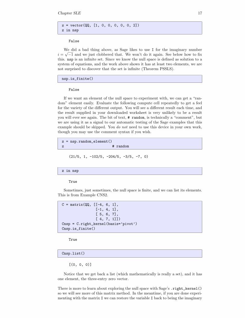
z = vector(QQ, [1, 0, 0, 0, 0, 0, 2])
z in nsp
False
We did a bad thing above, as Sage likes to use I for the imaginary numberi =√−1 and we just clobbered that. We won’t do it again. See below how to fix
this. nsp is an infinite set. Since we know the null space is defined as solution to asystem of equations, and the work above shows it has at least two elements, we arenot surprised to discover that the set is infinite (Theorem PSSLS).
nsp.is_finite()
False
If we want an element of the null space to experiment with, we can get a “ran-dom” element easily. Evaluate the following compute cell repeatedly to get a feelfor the variety of the different output. You will see a different result each time, andthe result supplied in your downloaded worksheet is very unlikely to be a resultyou will ever see again. The bit of text, # random, is technically a “comment”, butwe are using it as a signal to our automatic testing of the Sage examples that thisexample should be skipped. You do not need to use this device in your own work,though you may use the comment syntax if you wish.
z = nsp.random_element()
z # random
(21/5, 1, -102/5, -204/5, -3/5, -7, 0)
z in nsp
True
Sometimes, just sometimes, the null space is finite, and we can list its elements.This is from Example CNS2.
C = matrix(QQ, [[-4, 6, 1],
[-1, 4, 1],
[ 5, 6, 7],
[ 4, 7, 1]])
Cnsp = C.right_kernel(basis=’pivot’)
Cnsp.is_finite()
True
Cnsp.list()
[(0, 0, 0)]
Notice that we get back a list (which mathematically is really a set), and it hasone element, the three-entry zero vector.
There is more to learn about exploring the null space with Sage’s .right_kernel()so we will see more of this matrix method. In the meantime, if you are done experi-menting with the matrix I we can restore the variable I back to being the imaginary
Chapter SLE 18
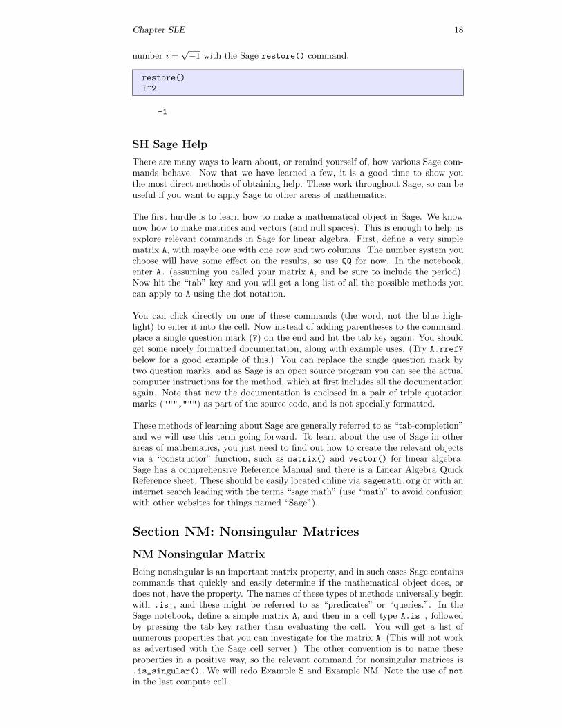
number i =√−1 with the Sage restore() command.
restore()
I^2
-1
SH Sage Help
There are many ways to learn about, or remind yourself of, how various Sage com-mands behave. Now that we have learned a few, it is a good time to show youthe most direct methods of obtaining help. These work throughout Sage, so can beuseful if you want to apply Sage to other areas of mathematics.
The first hurdle is to learn how to make a mathematical object in Sage. We knownow how to make matrices and vectors (and null spaces). This is enough to help usexplore relevant commands in Sage for linear algebra. First, define a very simplematrix A, with maybe one with one row and two columns. The number system youchoose will have some effect on the results, so use QQ for now. In the notebook,enter A. (assuming you called your matrix A, and be sure to include the period).Now hit the “tab” key and you will get a long list of all the possible methods youcan apply to A using the dot notation.
You can click directly on one of these commands (the word, not the blue high-light) to enter it into the cell. Now instead of adding parentheses to the command,place a single question mark (?) on the end and hit the tab key again. You shouldget some nicely formatted documentation, along with example uses. (Try A.rref?
below for a good example of this.) You can replace the single question mark bytwo question marks, and as Sage is an open source program you can see the actualcomputer instructions for the method, which at first includes all the documentationagain. Note that now the documentation is enclosed in a pair of triple quotationmarks (""",""") as part of the source code, and is not specially formatted.
These methods of learning about Sage are generally referred to as “tab-completion”and we will use this term going forward. To learn about the use of Sage in otherareas of mathematics, you just need to find out how to create the relevant objectsvia a “constructor” function, such as matrix() and vector() for linear algebra.Sage has a comprehensive Reference Manual and there is a Linear Algebra QuickReference sheet. These should be easily located online via sagemath.org or with aninternet search leading with the terms “sage math” (use “math” to avoid confusionwith other websites for things named “Sage”).
Section NM: Nonsingular Matrices
NM Nonsingular Matrix
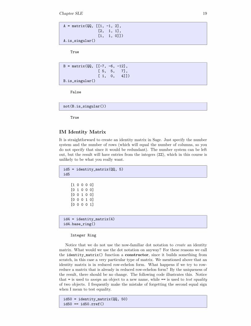
Being nonsingular is an important matrix property, and in such cases Sage containscommands that quickly and easily determine if the mathematical object does, ordoes not, have the property. The names of these types of methods universally beginwith .is_, and these might be referred to as “predicates” or “queries.”. In theSage notebook, define a simple matrix A, and then in a cell type A.is_, followedby pressing the tab key rather than evaluating the cell. You will get a list ofnumerous properties that you can investigate for the matrix A. (This will not workas advertised with the Sage cell server.) The other convention is to name theseproperties in a positive way, so the relevant command for nonsingular matrices is.is_singular(). We will redo Example S and Example NM. Note the use of notin the last compute cell.
Chapter SLE 19
A = matrix(QQ, [[1, -1, 2],
[2, 1, 1],
[1, 1, 0]])
A.is_singular()
True
B = matrix(QQ, [[-7, -6, -12],
[ 5, 5, 7],
[ 1, 0, 4]])
B.is_singular()
False
not(B.is_singular())
True
IM Identity Matrix
It is straightforward to create an identity matrix in Sage. Just specify the numbersystem and the number of rows (which will equal the number of columns, so youdo not specify that since it would be redundant). The number system can be leftout, but the result will have entries from the integers (ZZ), which in this course isunlikely to be what you really want.
id5 = identity_matrix(QQ, 5)
id5
[1 0 0 0 0]
[0 1 0 0 0]
[0 0 1 0 0]
[0 0 0 1 0]
[0 0 0 0 1]
id4 = identity_matrix(4)
id4.base_ring()
Integer Ring
Notice that we do not use the now-familiar dot notation to create an identitymatrix. What would we use the dot notation on anyway? For these reasons we callthe identity_matrix() function a constructor, since it builds something fromscratch, in this case a very particular type of matrix. We mentioned above that anidentity matrix is in reduced row-echelon form. What happens if we try to row-reduce a matrix that is already in reduced row-echelon form? By the uniqueness ofthe result, there should be no change. The following code illustrates this. Noticethat = is used to assign an object to a new name, while == is used to test equalityof two objects. I frequently make the mistake of forgetting the second equal signwhen I mean to test equality.
id50 = identity_matrix(QQ, 50)
id50 == id50.rref()
Chapter SLE 20
True
NME1 Nonsingular Matrix Equivalences, Round 1
Sage will create random matrices and vectors, sometimes with various properties.These can be very useful for quick experiments, and they are also useful for illus-trating that theorems hold for any object satisfying the hypotheses of the theorem.But this will never replace a proof.
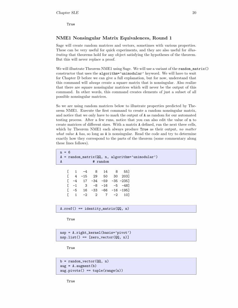
We will illustrate Theorem NME1 using Sage. We will use a variant of the random_matrix()constructor that uses the algorithm=’unimodular’ keyword. We will have to waitfor Chapter D before we can give a full explanation, but for now, understand thatthis command will always create a square matrix that is nonsingular. Also realizethat there are square nonsingular matrices which will never be the output of thiscommand. In other words, this command creates elements of just a subset of allpossible nonsingular matrices.
So we are using random matrices below to illustrate properties predicted by The-orem NME1. Execute the first command to create a random nonsingular matrix,and notice that we only have to mark the output of A as random for our automatedtesting process. After a few runs, notice that you can also edit the value of n tocreate matrices of different sizes. With a matrix A defined, run the next three cells,which by Theorem NME1 each always produce True as their output, no matterwhat value A has, so long as A is nonsingular. Read the code and try to determineexactly how they correspond to the parts of the theorem (some commentary alongthese lines follows).
n = 6
A = random_matrix(QQ, n, algorithm=’unimodular’)
A # random
[ 1 -4 8 14 8 55]
[ 4 -15 29 50 30 203]
[ -4 17 -34 -59 -35 -235]
[ -1 3 -8 -16 -5 -48]
[ -5 16 -33 -66 -16 -195]
[ 1 -2 2 7 -2 10]
A.rref() == identity_matrix(QQ, n)
True
nsp = A.right_kernel(basis=’pivot’)
nsp.list() == [zero_vector(QQ, n)]
True
b = random_vector(QQ, n)
aug = A.augment(b)
aug.pivots() == tuple(range(n))
True
Chapter SLE 21
The only portion of these commands that may be unfamilar is the last one. Thecommand range(n) is incredibly useful, as it will create a list of the integers from0 up to, but not including, n. (We saw this command briefly in Sage FDV.) So, forexample, range(3) == [0,1,2] is True. Pivots are returned as a “tuple” whichis very much like a list, except we cannot change the contents. We can see thedifference by the way the tuple prints with parentheses ((,)) rather than brackets([,]). We can convert a list to a tuple with the tuple() command, in order tomake the comparison succeed.
How do we tell if the reduced row-echelon form of the augmented matrix of a systemof equations represents a system with a unique solution? First, the system must beconsistent, which by Theorem RCLS means the last column is not a pivot column.Then with a consistent system we need to insure there are no free variables. Thishappens if and only if the remaining columns are all pivot columns, according toTheorem FVCS, thus the test used in the last compute cell.
Chapter VVectors
Section VO: Vector Operations
VSCV Vector Spaces of Column Vectors
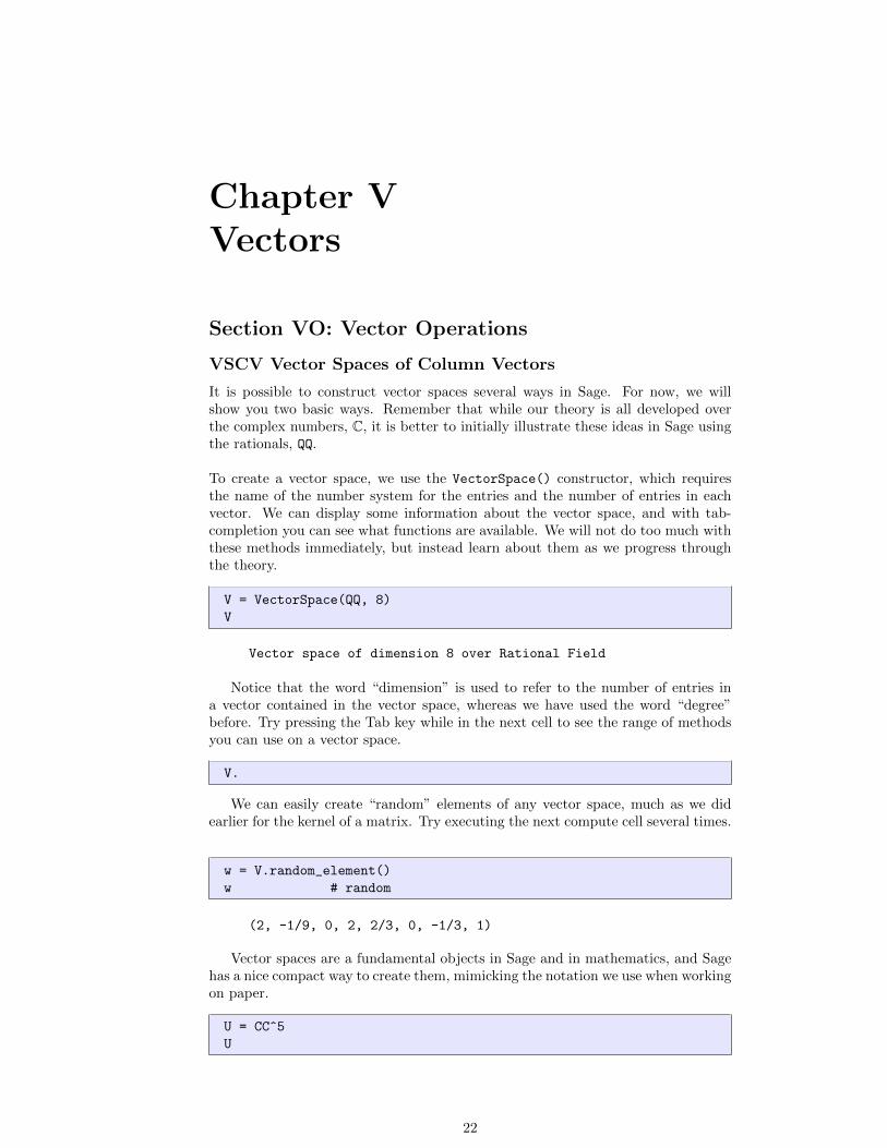
It is possible to construct vector spaces several ways in Sage. For now, we willshow you two basic ways. Remember that while our theory is all developed overthe complex numbers, C, it is better to initially illustrate these ideas in Sage usingthe rationals, QQ.
To create a vector space, we use the VectorSpace() constructor, which requiresthe name of the number system for the entries and the number of entries in eachvector. We can display some information about the vector space, and with tab-completion you can see what functions are available. We will not do too much withthese methods immediately, but instead learn about them as we progress throughthe theory.
V = VectorSpace(QQ, 8)
V
Vector space of dimension 8 over Rational Field
Notice that the word “dimension” is used to refer to the number of entries ina vector contained in the vector space, whereas we have used the word “degree”before. Try pressing the Tab key while in the next cell to see the range of methodsyou can use on a vector space.
V.
We can easily create “random” elements of any vector space, much as we didearlier for the kernel of a matrix. Try executing the next compute cell several times.
w = V.random_element()
w # random
(2, -1/9, 0, 2, 2/3, 0, -1/3, 1)
Vector spaces are a fundamental objects in Sage and in mathematics, and Sagehas a nice compact way to create them, mimicking the notation we use when workingon paper.
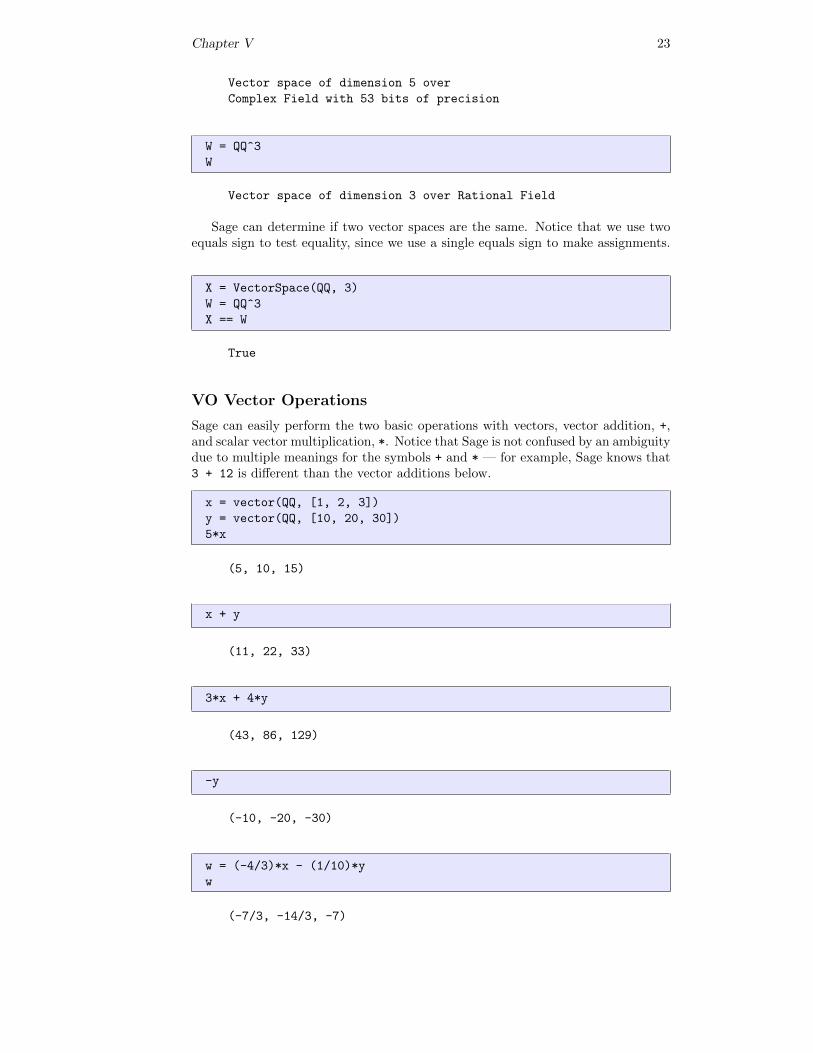
U = CC^5
U
22
Chapter V 23
Vector space of dimension 5 over
Complex Field with 53 bits of precision
W = QQ^3
W
Vector space of dimension 3 over Rational Field
Sage can determine if two vector spaces are the same. Notice that we use twoequals sign to test equality, since we use a single equals sign to make assignments.
X = VectorSpace(QQ, 3)
W = QQ^3
X == W
True
VO Vector Operations
Sage can easily perform the two basic operations with vectors, vector addition, +,and scalar vector multiplication, *. Notice that Sage is not confused by an ambiguitydue to multiple meanings for the symbols + and * — for example, Sage knows that3 + 12 is different than the vector additions below.
x = vector(QQ, [1, 2, 3])
y = vector(QQ, [10, 20, 30])
5*x
(5, 10, 15)
x + y
(11, 22, 33)
3*x + 4*y
(43, 86, 129)
-y
(-10, -20, -30)
w = (-4/3)*x - (1/10)*y
w
(-7/3, -14/3, -7)
Chapter V 24
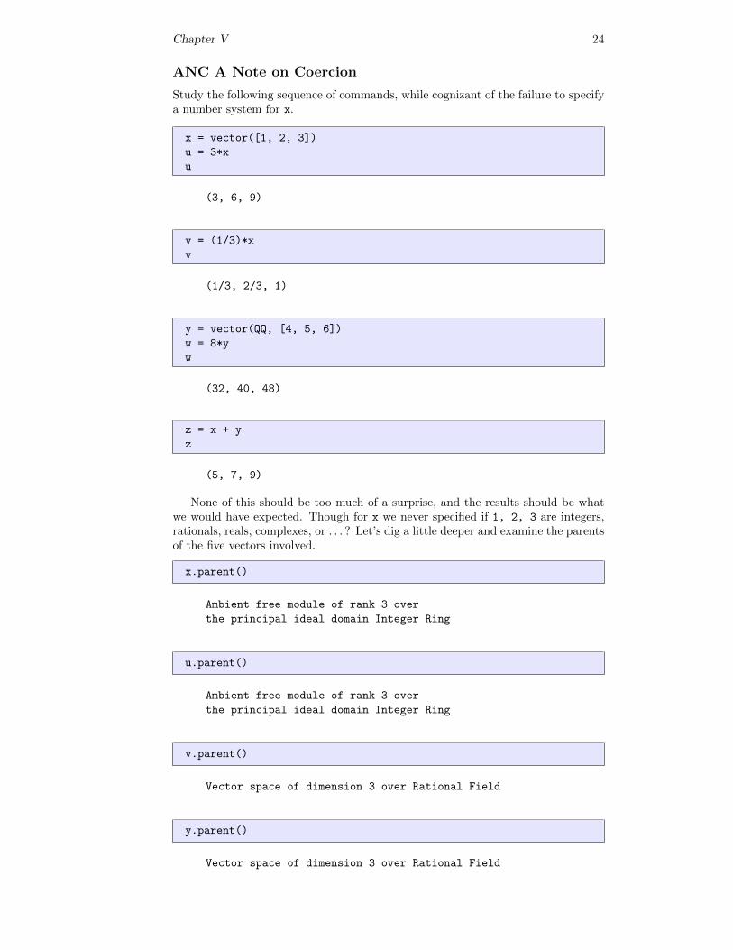
ANC A Note on Coercion
Study the following sequence of commands, while cognizant of the failure to specifya number system for x.
x = vector([1, 2, 3])
u = 3*x
u
(3, 6, 9)
v = (1/3)*x
v
(1/3, 2/3, 1)
y = vector(QQ, [4, 5, 6])
w = 8*y
w
(32, 40, 48)
z = x + y
z
(5, 7, 9)
None of this should be too much of a surprise, and the results should be whatwe would have expected. Though for x we never specified if 1, 2, 3 are integers,rationals, reals, complexes, or . . . ? Let’s dig a little deeper and examine the parentsof the five vectors involved.
x.parent()
Ambient free module of rank 3 over
the principal ideal domain Integer Ring
u.parent()
Ambient free module of rank 3 over
the principal ideal domain Integer Ring
v.parent()
Vector space of dimension 3 over Rational Field
y.parent()
Vector space of dimension 3 over Rational Field
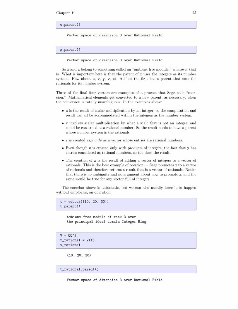
Chapter V 25
w.parent()
Vector space of dimension 3 over Rational Field
z.parent()
Vector space of dimension 3 over Rational Field
So x and u belong to something called an “ambient free module,” whatever thatis. What is important here is that the parent of x uses the integers as its numbersystem. How about u, v, y, w, z? All but the first has a parent that uses therationals for its number system.
Three of the final four vectors are examples of a process that Sage calls “coer-cion.” Mathematical elements get converted to a new parent, as necessary, whenthe conversion is totally unambiguous. In the examples above:
• u is the result of scalar multiplication by an integer, so the computation andresult can all be accommodated within the integers as the number system.
• v involves scalar multiplication by what a scalr that is not an integer, andcould be construed as a rational number. So the result needs to have a parentwhose number system is the rationals.
• y is created explicitly as a vector whose entries are rational numbers.
• Even though w is created only with products of integers, the fact that y hasentries considered as rational numbers, so too does the result.
• The creation of z is the result of adding a vector of integers to a vector ofrationals. This is the best example of coercion — Sage promotes x to a vectorof rationals and therefore returns a result that is a vector of rationals. Noticethat there is no ambiguity and no argument about how to promote x, and thesame would be true for any vector full of integers.
The coercion above is automatic, but we can also usually force it to happenwithout employing an operation.
t = vector([10, 20, 30])
t.parent()
Ambient free module of rank 3 over
the principal ideal domain Integer Ring
V = QQ^3
t_rational = V(t)
t_rational
(10, 20, 30)
t_rational.parent()
Vector space of dimension 3 over Rational Field
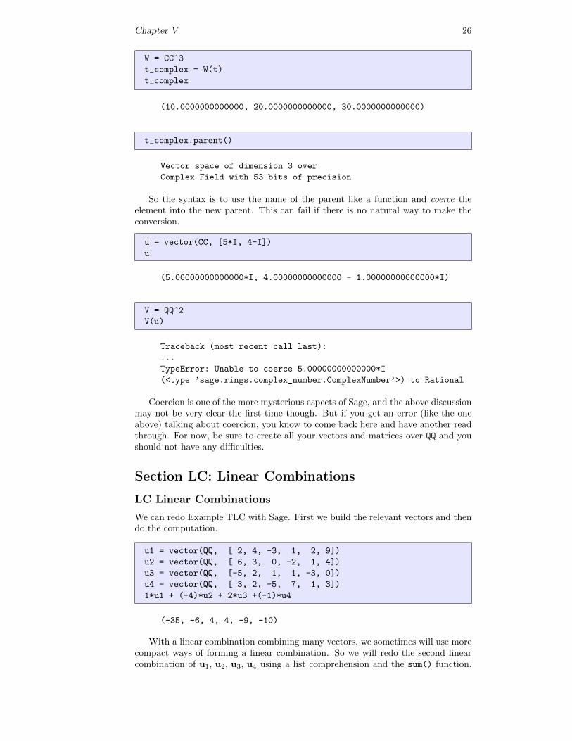
Chapter V 26
W = CC^3
t_complex = W(t)
t_complex
(10.0000000000000, 20.0000000000000, 30.0000000000000)
t_complex.parent()
Vector space of dimension 3 over
Complex Field with 53 bits of precision
So the syntax is to use the name of the parent like a function and coerce theelement into the new parent. This can fail if there is no natural way to make theconversion.
u = vector(CC, [5*I, 4-I])
u
(5.00000000000000*I, 4.00000000000000 - 1.00000000000000*I)
V = QQ^2
V(u)
Traceback (most recent call last):
...
TypeError: Unable to coerce 5.00000000000000*I
(<type ’sage.rings.complex_number.ComplexNumber’>) to Rational
Coercion is one of the more mysterious aspects of Sage, and the above discussionmay not be very clear the first time though. But if you get an error (like the oneabove) talking about coercion, you know to come back here and have another readthrough. For now, be sure to create all your vectors and matrices over QQ and youshould not have any difficulties.
Section LC: Linear Combinations
LC Linear Combinations
We can redo Example TLC with Sage. First we build the relevant vectors and thendo the computation.
u1 = vector(QQ, [ 2, 4, -3, 1, 2, 9])
u2 = vector(QQ, [ 6, 3, 0, -2, 1, 4])
u3 = vector(QQ, [-5, 2, 1, 1, -3, 0])
u4 = vector(QQ, [ 3, 2, -5, 7, 1, 3])
1*u1 + (-4)*u2 + 2*u3 +(-1)*u4
(-35, -6, 4, 4, -9, -10)
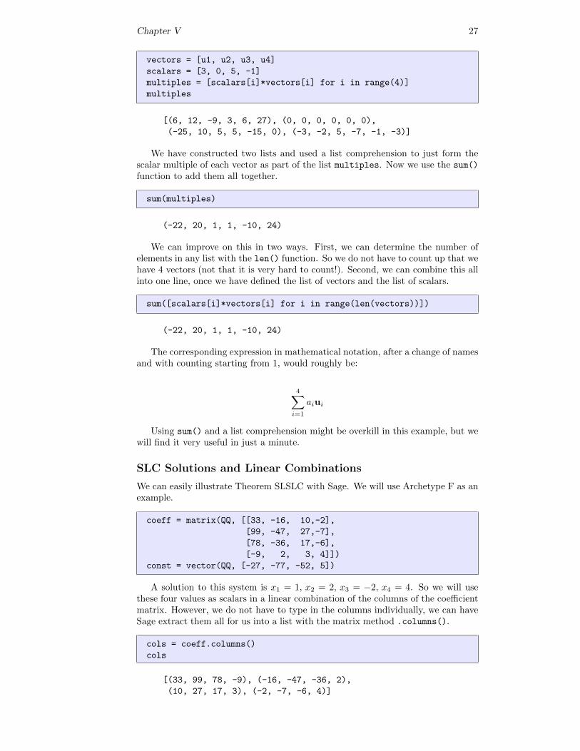
With a linear combination combining many vectors, we sometimes will use morecompact ways of forming a linear combination. So we will redo the second linearcombination of u1, u2, u3, u4 using a list comprehension and the sum() function.
Chapter V 27
vectors = [u1, u2, u3, u4]
scalars = [3, 0, 5, -1]
multiples = [scalars[i]*vectors[i] for i in range(4)]
multiples
[(6, 12, -9, 3, 6, 27), (0, 0, 0, 0, 0, 0),
(-25, 10, 5, 5, -15, 0), (-3, -2, 5, -7, -1, -3)]
We have constructed two lists and used a list comprehension to just form thescalar multiple of each vector as part of the list multiples. Now we use the sum()
function to add them all together.
sum(multiples)
(-22, 20, 1, 1, -10, 24)
We can improve on this in two ways. First, we can determine the number ofelements in any list with the len() function. So we do not have to count up that wehave 4 vectors (not that it is very hard to count!). Second, we can combine this allinto one line, once we have defined the list of vectors and the list of scalars.
sum([scalars[i]*vectors[i] for i in range(len(vectors))])
(-22, 20, 1, 1, -10, 24)
The corresponding expression in mathematical notation, after a change of namesand with counting starting from 1, would roughly be:
4∑i=1
aiui
Using sum() and a list comprehension might be overkill in this example, but wewill find it very useful in just a minute.
SLC Solutions and Linear Combinations
We can easily illustrate Theorem SLSLC with Sage. We will use Archetype F as anexample.
coeff = matrix(QQ, [[33, -16, 10,-2],
[99, -47, 27,-7],
[78, -36, 17,-6],
[-9, 2, 3, 4]])
const = vector(QQ, [-27, -77, -52, 5])
A solution to this system is x1 = 1, x2 = 2, x3 = −2, x4 = 4. So we will usethese four values as scalars in a linear combination of the columns of the coefficientmatrix. However, we do not have to type in the columns individually, we can haveSage extract them all for us into a list with the matrix method .columns().
cols = coeff.columns()
cols
[(33, 99, 78, -9), (-16, -47, -36, 2),
(10, 27, 17, 3), (-2, -7, -6, 4)]
Chapter V 28
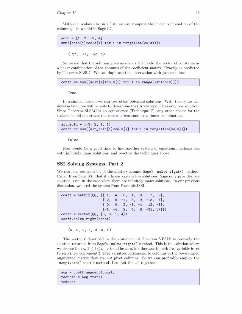
With our scalars also in a list, we can compute the linear combination of thecolumns, like we did in Sage LC.
soln = [1, 2, -2, 4]
sum([soln[i]*cols[i] for i in range(len(cols))])
(-27, -77, -52, 5)
So we see that the solution gives us scalars that yield the vector of constants asa linear combination of the columns of the coefficient matrix. Exactly as predictedby Theorem SLSLC. We can duplicate this observation with just one line:
const == sum([soln[i]*cols[i] for i in range(len(cols))])
True
In a similar fashion we can test other potential solutions. With theory we willdevelop later, we will be able to determine that Archetype F has only one solution.Since Theorem SLSLC is an equivalence (Technique E), any other choice for thescalars should not create the vector of constants as a linear combination.
alt_soln = [-3, 2, 4, 1]
const == sum([alt_soln[i]*cols[i] for i in range(len(cols))])
False
Now would be a good time to find another system of equations, perhaps onewith infinitely many solutions, and practice the techniques above.
SS2 Solving Systems, Part 2
We can now resolve a bit of the mystery around Sage’s .solve_right() method.Recall from Sage SS1 that if a linear system has solutions, Sage only provides onesolution, even in the case when there are infinitely many solutions. In our previousdiscussion, we used the system from Example ISSI.
coeff = matrix(QQ, [[ 1, 4, 0, -1, 0, 7, -9],
[ 2, 8, -1, 3, 9, -13, 7],
[ 0, 0, 2, -3, -4, 12, -8],
[-1, -4, 2, 4, 8, -31, 37]])
const = vector(QQ, [3, 9, 1, 4])
coeff.solve_right(const)
(4, 0, 2, 1, 0, 0, 0)
The vector c described in the statement of Theorem VFSLS is precisely thesolution returned from Sage’s .solve_right() method. This is the solution wherewe choose the αi, 1 ≤ i ≤ n−r to all be zero, in other words, each free variable is setto zero (how convenient!). Free variables correspond to columns of the row-reducedaugmented matrix that are not pivot columns. So we can profitably employ the.nonpivots() matrix method. Lets put this all together.
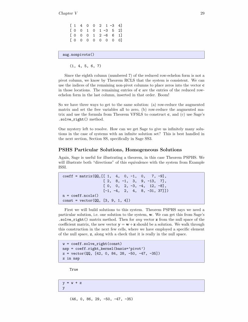
aug = coeff.augment(const)
reduced = aug.rref()
reduced
Chapter V 29
[ 1 4 0 0 2 1 -3 4]
[ 0 0 1 0 1 -3 5 2]
[ 0 0 0 1 2 -6 6 1]
[ 0 0 0 0 0 0 0 0]
aug.nonpivots()
(1, 4, 5, 6, 7)
Since the eighth column (numbered 7) of the reduced row-echelon form is not apivot column, we know by Theorem RCLS that the system is consistent. We canuse the indices of the remaining non-pivot columns to place zeros into the vector cin those locations. The remaining entries of c are the entries of the reduced row-echelon form in the last column, inserted in that order. Boom!
So we have three ways to get to the same solution: (a) row-reduce the augmentedmatrix and set the free variables all to zero, (b) row-reduce the augmented ma-trix and use the formula from Theorem VFSLS to construct c, and (c) use Sage’s.solve_right() method.
One mystery left to resolve. How can we get Sage to give us infinitely many solu-tions in the case of systems with an infinite solution set? This is best handled inthe next section, Section SS, specifically in Sage SS3.
PSHS Particular Solutions, Homogeneous Solutions
Again, Sage is useful for illustrating a theorem, in this case Theorem PSPHS. Wewill illustrate both “directions” of this equivalence with the system from ExampleISSI.
coeff = matrix(QQ,[[ 1, 4, 0, -1, 0, 7, -9],
[ 2, 8, -1, 3, 9, -13, 7],
[ 0, 0, 2, -3, -4, 12, -8],
[-1, -4, 2, 4, 8, -31, 37]])
n = coeff.ncols()
const = vector(QQ, [3, 9, 1, 4])
First we will build solutions to this system. Theorem PSPHS says we need aparticular solution, i.e. one solution to the system, w. We can get this from Sage’s.solve_right() matrix method. Then for any vector z from the null space of thecoefficient matrix, the new vector y = w+z should be a solution. We walk throughthis construction in the next few cells, where we have employed a specific elementof the null space, z, along with a check that it is really in the null space.
w = coeff.solve_right(const)
nsp = coeff.right_kernel(basis=’pivot’)
z = vector(QQ, [42, 0, 84, 28, -50, -47, -35])
z in nsp
True
y = w + z
y
(46, 0, 86, 29, -50, -47, -35)
Chapter V 30
const == sum([y[i]*coeff.column(i) for i in range(n)])
True
You can create solutions repeatedly via the creation of random elements of thenull space. Be sure you have executed the cells above, so that coeff, n, const,nsp and w are all defined. Try executing the cell below repeatedly to test infinitelymany solutions to the system. You can use the subsequent compute cell to peek atany of the solutions you create.
z = nsp.random_element()
y = w + z
const == sum([y[i]*coeff.column(i) for i in range(n)])
True
y # random
(-11/2, 0, 45/2, 34, 0, 7/2, -2)
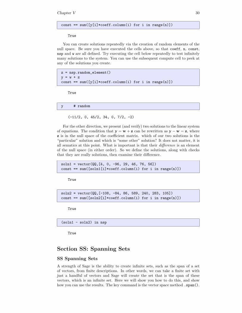
For the other direction, we present (and verify) two solutions to the linear systemof equations. The condition that y = w + z can be rewritten as y −w = z, wherez is in the null space of the coefficient matrix. which of our two solutions is the“particular” solution and which is “some other” solution? It does not matter, it isall sematics at this point. What is important is that their difference is an elementof the null space (in either order). So we define the solutions, along with checksthat they are really solutions, then examine their difference.
soln1 = vector(QQ,[4, 0, -96, 29, 46, 76, 56])
const == sum([soln1[i]*coeff.column(i) for i in range(n)])
True
soln2 = vector(QQ,[-108, -84, 86, 589, 240, 283, 105])
const == sum([soln2[i]*coeff.column(i) for i in range(n)])
True
(soln1 - soln2) in nsp
True
Section SS: Spanning Sets
SS Spanning Sets
A strength of Sage is the ability to create infinite sets, such as the span of a setof vectors, from finite descriptions. In other words, we can take a finite set withjust a handful of vectors and Sage will create the set that is the span of thesevectors, which is an infinite set. Here we will show you how to do this, and showhow you can use the results. The key command is the vector space method .span().
Chapter V 31
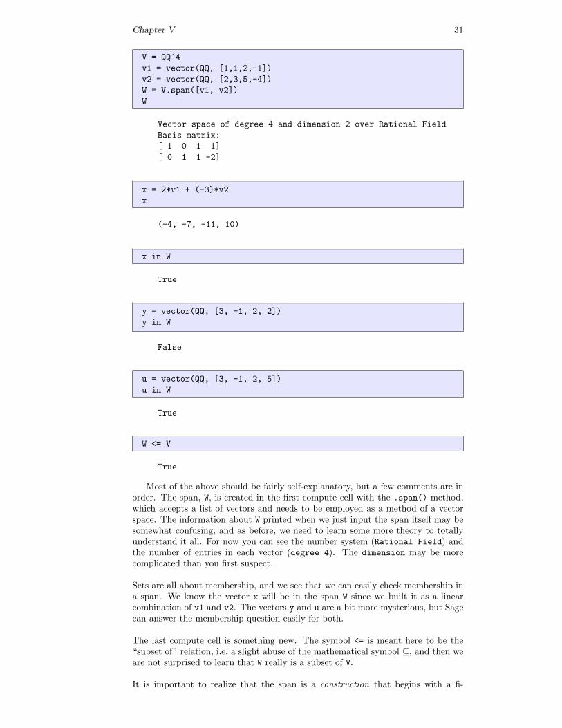
V = QQ^4
v1 = vector(QQ, [1,1,2,-1])
v2 = vector(QQ, [2,3,5,-4])
W = V.span([v1, v2])
W
Vector space of degree 4 and dimension 2 over Rational Field
Basis matrix:
[ 1 0 1 1]
[ 0 1 1 -2]
x = 2*v1 + (-3)*v2
x
(-4, -7, -11, 10)
x in W
True
y = vector(QQ, [3, -1, 2, 2])
y in W
False
u = vector(QQ, [3, -1, 2, 5])
u in W
True
W <= V
True
Most of the above should be fairly self-explanatory, but a few comments are inorder. The span, W, is created in the first compute cell with the .span() method,which accepts a list of vectors and needs to be employed as a method of a vectorspace. The information about W printed when we just input the span itself may besomewhat confusing, and as before, we need to learn some more theory to totallyunderstand it all. For now you can see the number system (Rational Field) andthe number of entries in each vector (degree 4). The dimension may be morecomplicated than you first suspect.
Sets are all about membership, and we see that we can easily check membership ina span. We know the vector x will be in the span W since we built it as a linearcombination of v1 and v2. The vectors y and u are a bit more mysterious, but Sagecan answer the membership question easily for both.
The last compute cell is something new. The symbol <= is meant here to be the“subset of” relation, i.e. a slight abuse of the mathematical symbol ⊆, and then weare not surprised to learn that W really is a subset of V.
It is important to realize that the span is a construction that begins with a fi-
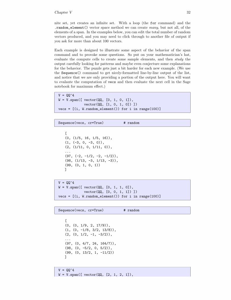
Chapter V 32
nite set, yet creates an infinite set. With a loop (the for command) and the.random_element() vector space method we can create many, but not all, of theelements of a span. In the examples below, you can edit the total number of randomvectors produced, and you may need to click through to another file of output ifyou ask for more than about 100 vectors.
Each example is designed to illustrate some aspect of the behavior of the spancommand and to provoke some questions. So put on your mathematician’s hat,evaluate the compute cells to create some sample elements, and then study theoutput carefully looking for patterns and maybe even conjecture some explanationsfor the behavior. The puzzle gets just a bit harder for each new example. (We usethe Sequence() command to get nicely-formatted line-by-line output of the list,and notice that we are only providing a portion of the output here. You will wantto evalaute the computation of vecs and then evaluate the next cell in the Sagenotebook for maximum effect.)
V = QQ^4
W = V.span([ vector(QQ, [0, 1, 0, 1]),
vector(QQ, [1, 0, 1, 0]) ])
vecs = [(i, W.random_element()) for i in range(100)]
Sequence(vecs, cr=True) # random
[
(0, (1/5, 16, 1/5, 16)),
(1, (-3, 0, -3, 0)),
(2, (1/11, 0, 1/11, 0)),
...
(97, (-2, -1/2, -2, -1/2)),
(98, (1/13, -3, 1/13, -3)),
(99, (0, 1, 0, 1))
]
V = QQ^4
W = V.span([ vector(QQ, [0, 1, 1, 0]),
vector(QQ, [0, 0, 1, 1]) ])
vecs = [(i, W.random_element()) for i in range(100)]
Sequence(vecs, cr=True) # random
[
(0, (0, 1/9, 2, 17/9)),
(1, (0, -1/8, 3/2, 13/8)),
(2, (0, 1/2, -1, -3/2)),
...
(97, (0, 4/7, 24, 164/7)),
(98, (0, -5/2, 0, 5/2)),
(99, (0, 13/2, 1, -11/2))
]
V = QQ^4
W = V.span([ vector(QQ, [2, 1, 2, 1]),
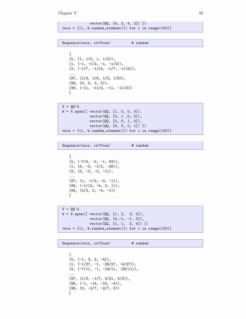
Chapter V 33
vector(QQ, [4, 2, 4, 2]) ])
vecs = [(i, W.random_element()) for i in range(100)]
Sequence(vecs, cr=True) # random
[
(0, (1, 1/2, 1, 1/2)),
(1, (-1, -1/2, -1, -1/2)),
(2, (-1/7, -1/14, -1/7, -1/14)),
...
(97, (1/3, 1/6, 1/3, 1/6)),
(98, (0, 0, 0, 0)),
(99, (-11, -11/2, -11, -11/2))
]
V = QQ^4
W = V.span([ vector(QQ, [1, 0, 0, 0]),
vector(QQ, [0, 1 ,0, 0]),
vector(QQ, [0, 0, 1, 0]),
vector(QQ, [0, 0, 0, 1]) ])
vecs = [(i, W.random_element()) for i in range(100)]
Sequence(vecs, cr=True) # random
[
(0, (-7/4, -2, -1, 63)),
(1, (6, -2, -1/2, -28)),
(2, (5, -2, -2, -1)),
...
(97, (1, -1/2, -2, -1)),
(98, (-1/12, -4, 2, 1)),
(99, (2/3, 0, -4, -1))
]
V = QQ^4
W = V.span([ vector(QQ, [1, 2, 3, 4]),
vector(QQ, [0,-1, -1, 0]),
vector(QQ, [1, 1, 2, 4]) ])
vecs = [(i, W.random_element()) for i in range(100)]
Sequence(vecs, cr=True) # random
[
(0, (-1, 3, 2, -4)),
(1, (-1/27, -1, -28/27, -4/27)),
(2, (-7/11, -1, -18/11, -28/11)),
...
(97, (1/3, -1/7, 4/21, 4/3)),
(98, (-1, -14, -15, -4)),
(99, (0, -2/7, -2/7, 0))
]
Chapter V 34
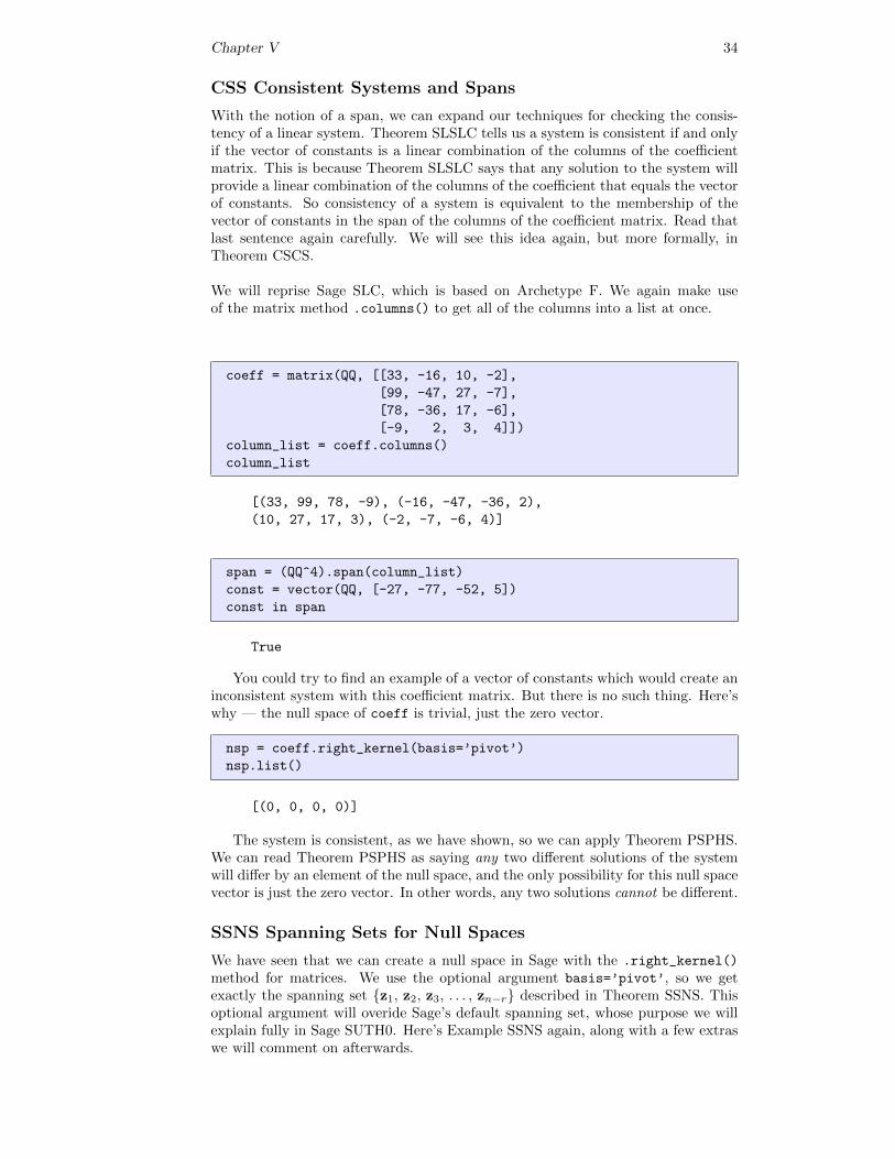
CSS Consistent Systems and Spans
With the notion of a span, we can expand our techniques for checking the consis-tency of a linear system. Theorem SLSLC tells us a system is consistent if and onlyif the vector of constants is a linear combination of the columns of the coefficientmatrix. This is because Theorem SLSLC says that any solution to the system willprovide a linear combination of the columns of the coefficient that equals the vectorof constants. So consistency of a system is equivalent to the membership of thevector of constants in the span of the columns of the coefficient matrix. Read thatlast sentence again carefully. We will see this idea again, but more formally, inTheorem CSCS.
We will reprise Sage SLC, which is based on Archetype F. We again make useof the matrix method .columns() to get all of the columns into a list at once.
coeff = matrix(QQ, [[33, -16, 10, -2],
[99, -47, 27, -7],
[78, -36, 17, -6],
[-9, 2, 3, 4]])
column_list = coeff.columns()
column_list
[(33, 99, 78, -9), (-16, -47, -36, 2),
(10, 27, 17, 3), (-2, -7, -6, 4)]
span = (QQ^4).span(column_list)
const = vector(QQ, [-27, -77, -52, 5])
const in span
True
You could try to find an example of a vector of constants which would create aninconsistent system with this coefficient matrix. But there is no such thing. Here’swhy — the null space of coeff is trivial, just the zero vector.
nsp = coeff.right_kernel(basis=’pivot’)
nsp.list()
[(0, 0, 0, 0)]
The system is consistent, as we have shown, so we can apply Theorem PSPHS.We can read Theorem PSPHS as saying any two different solutions of the systemwill differ by an element of the null space, and the only possibility for this null spacevector is just the zero vector. In other words, any two solutions cannot be different.
SSNS Spanning Sets for Null Spaces
We have seen that we can create a null space in Sage with the .right_kernel()
method for matrices. We use the optional argument basis=’pivot’, so we getexactly the spanning set {z1, z2, z3, . . . , zn−r} described in Theorem SSNS. Thisoptional argument will overide Sage’s default spanning set, whose purpose we willexplain fully in Sage SUTH0. Here’s Example SSNS again, along with a few extraswe will comment on afterwards.
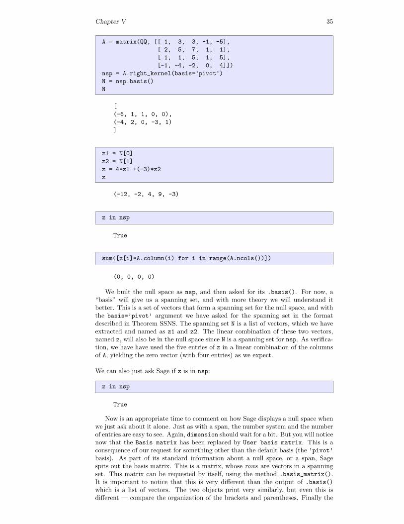
Chapter V 35
A = matrix(QQ, [[ 1, 3, 3, -1, -5],
[ 2, 5, 7, 1, 1],
[ 1, 1, 5, 1, 5],
[-1, -4, -2, 0, 4]])
nsp = A.right_kernel(basis=’pivot’)
N = nsp.basis()
N
[
(-6, 1, 1, 0, 0),
(-4, 2, 0, -3, 1)
]
z1 = N[0]
z2 = N[1]
z = 4*z1 +(-3)*z2
z
(-12, -2, 4, 9, -3)
z in nsp
True
sum([z[i]*A.column(i) for i in range(A.ncols())])
(0, 0, 0, 0)
We built the null space as nsp, and then asked for its .basis(). For now, a“basis” will give us a spanning set, and with more theory we will understand itbetter. This is a set of vectors that form a spanning set for the null space, and withthe basis=’pivot’ argument we have asked for the spanning set in the formatdescribed in Theorem SSNS. The spanning set N is a list of vectors, which we haveextracted and named as z1 and z2. The linear combination of these two vectors,named z, will also be in the null space since N is a spanning set for nsp. As verifica-tion, we have have used the five entries of z in a linear combination of the columnsof A, yielding the zero vector (with four entries) as we expect.
We can also just ask Sage if z is in nsp:
z in nsp
True
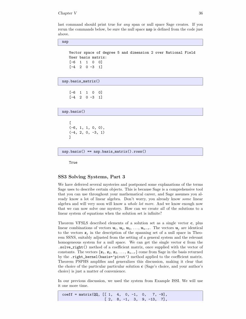
Now is an appropriate time to comment on how Sage displays a null space whenwe just ask about it alone. Just as with a span, the number system and the numberof entries are easy to see. Again, dimension should wait for a bit. But you will noticenow that the Basis matrix has been replaced by User basis matrix. This is aconsequence of our request for something other than the default basis (the ’pivot’
basis). As part of its standard information about a null space, or a span, Sagespits out the basis matrix. This is a matrix, whose rows are vectors in a spanningset. This matrix can be requested by itself, using the method .basis_matrix().It is important to notice that this is very different than the output of .basis()
which is a list of vectors. The two objects print very similarly, but even this isdifferent — compare the organization of the brackets and parentheses. Finally the
Chapter V 36
last command should print true for any span or null space Sage creates. If yourerun the commands below, be sure the null space nsp is defined from the code justabove.
nsp
Vector space of degree 5 and dimension 2 over Rational Field
User basis matrix:
[-6 1 1 0 0]
[-4 2 0 -3 1]
nsp.basis_matrix()
[-6 1 1 0 0]
[-4 2 0 -3 1]
nsp.basis()
[
(-6, 1, 1, 0, 0),
(-4, 2, 0, -3, 1)
]
nsp.basis() == nsp.basis_matrix().rows()
True
SS3 Solving Systems, Part 3
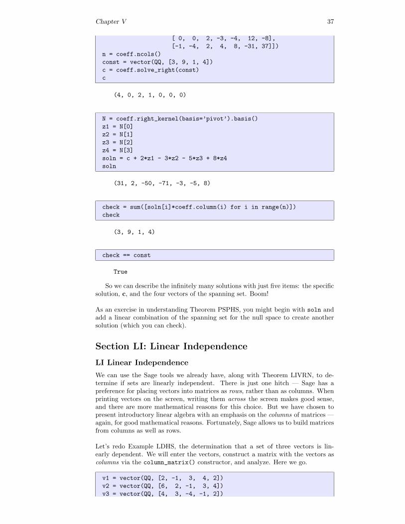
We have deferred several mysteries and postponed some explanations of the termsSage uses to describe certain objects. This is because Sage is a comprehensive toolthat you can use throughout your mathematical career, and Sage assumes you al-ready know a lot of linear algebra. Don’t worry, you already know some linearalgebra and will very soon will know a whole lot more. And we know enough nowthat we can now solve one mystery. How can we create all of the solutions to alinear system of equations when the solution set is infinite?
Theorem VFSLS described elements of a solution set as a single vector c, pluslinear combinations of vectors u1, u2, u3, . . . , un−r. The vectors uj are identicalto the vectors zj in the description of the spanning set of a null space in Theo-rem SSNS, suitably adjusted from the setting of a general system and the relevanthomogeneous system for a null space. We can get the single vector c from the.solve_right() method of a coefficient matrix, once supplied with the vector ofconstants. The vectors {z1, z2, z3, . . . , zn−r} come from Sage in the basis returnedby the .right_kernel(basis=’pivot’) method applied to the coefficient matrix.Theorem PSPHS amplifies and generalizes this discussion, making it clear thatthe choice of the particular particular solution c (Sage’s choice, and your author’schoice) is just a matter of convenience.
In our previous discussion, we used the system from Example ISSI. We will useit one more time.
coeff = matrix(QQ, [[ 1, 4, 0, -1, 0, 7, -9],
[ 2, 8, -1, 3, 9, -13, 7],
Chapter V 37
[ 0, 0, 2, -3, -4, 12, -8],
[-1, -4, 2, 4, 8, -31, 37]])
n = coeff.ncols()
const = vector(QQ, [3, 9, 1, 4])
c = coeff.solve_right(const)
c
(4, 0, 2, 1, 0, 0, 0)
N = coeff.right_kernel(basis=’pivot’).basis()
z1 = N[0]
z2 = N[1]
z3 = N[2]
z4 = N[3]
soln = c + 2*z1 - 3*z2 - 5*z3 + 8*z4
soln
(31, 2, -50, -71, -3, -5, 8)
check = sum([soln[i]*coeff.column(i) for i in range(n)])
check
(3, 9, 1, 4)
check == const
True
So we can describe the infinitely many solutions with just five items: the specificsolution, c, and the four vectors of the spanning set. Boom!
As an exercise in understanding Theorem PSPHS, you might begin with soln andadd a linear combination of the spanning set for the null space to create anothersolution (which you can check).
Section LI: Linear Independence
LI Linear Independence
We can use the Sage tools we already have, along with Theorem LIVRN, to de-termine if sets are linearly independent. There is just one hitch — Sage has apreference for placing vectors into matrices as rows, rather than as columns. Whenprinting vectors on the screen, writing them across the screen makes good sense,and there are more mathematical reasons for this choice. But we have chosen topresent introductory linear algebra with an emphasis on the columns of matrices —again, for good mathematical reasons. Fortunately, Sage allows us to build matricesfrom columns as well as rows.
Let’s redo Example LDHS, the determination that a set of three vectors is lin-early dependent. We will enter the vectors, construct a matrix with the vectors ascolumns via the column_matrix() constructor, and analyze. Here we go.
v1 = vector(QQ, [2, -1, 3, 4, 2])
v2 = vector(QQ, [6, 2, -1, 3, 4])
v3 = vector(QQ, [4, 3, -4, -1, 2])
Chapter V 38
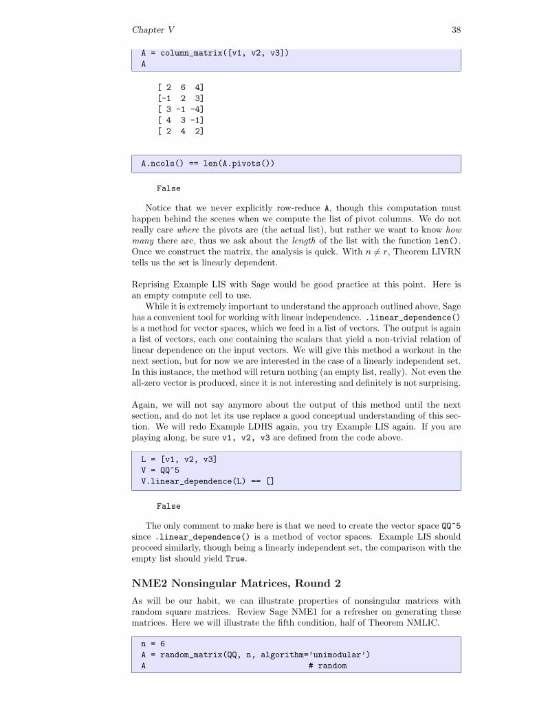
A = column_matrix([v1, v2, v3])
A
[ 2 6 4]
[-1 2 3]
[ 3 -1 -4]
[ 4 3 -1]
[ 2 4 2]
A.ncols() == len(A.pivots())
False
Notice that we never explicitly row-reduce A, though this computation musthappen behind the scenes when we compute the list of pivot columns. We do notreally care where the pivots are (the actual list), but rather we want to know howmany there are, thus we ask about the length of the list with the function len().Once we construct the matrix, the analysis is quick. With n 6= r, Theorem LIVRNtells us the set is linearly dependent.
Reprising Example LIS with Sage would be good practice at this point. Here isan empty compute cell to use.
While it is extremely important to understand the approach outlined above, Sagehas a convenient tool for working with linear independence. .linear_dependence()is a method for vector spaces, which we feed in a list of vectors. The output is againa list of vectors, each one containing the scalars that yield a non-trivial relation oflinear dependence on the input vectors. We will give this method a workout in thenext section, but for now we are interested in the case of a linearly independent set.In this instance, the method will return nothing (an empty list, really). Not even theall-zero vector is produced, since it is not interesting and definitely is not surprising.
Again, we will not say anymore about the output of this method until the nextsection, and do not let its use replace a good conceptual understanding of this sec-tion. We will redo Example LDHS again, you try Example LIS again. If you areplaying along, be sure v1, v2, v3 are defined from the code above.
L = [v1, v2, v3]
V = QQ^5
V.linear_dependence(L) == []
False
The only comment to make here is that we need to create the vector space QQ^5
since .linear_dependence() is a method of vector spaces. Example LIS shouldproceed similarly, though being a linearly independent set, the comparison with theempty list should yield True.
NME2 Nonsingular Matrices, Round 2
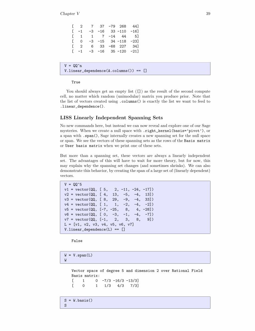
As will be our habit, we can illustrate properties of nonsingular matrices withrandom square matrices. Review Sage NME1 for a refresher on generating thesematrices. Here we will illustrate the fifth condition, half of Theorem NMLIC.
n = 6
A = random_matrix(QQ, n, algorithm=’unimodular’)
A # random
Chapter V 39
[ 2 7 37 -79 268 44]
[ -1 -3 -16 33 -110 -16]
[ 1 1 7 -14 44 5]
[ 0 -3 -15 34 -118 -23]
[ 2 6 33 -68 227 34]
[ -1 -3 -16 35 -120 -21]
V = QQ^n
V.linear_dependence(A.columns()) == []
True
You should always get an empty list ([]) as the result of the second computecell, no matter which random (unimodular) matrix you produce prior. Note thatthe list of vectors created using .columns() is exactly the list we want to feed to.linear_dependence().
LISS Linearly Independent Spanning Sets
No new commands here, but instead we can now reveal and explore one of our Sagemysteries. When we create a null space with .right_kernel(basis=’pivot’), ora span with .span(), Sage internally creates a new spanning set for the null spaceor span. We see the vectors of these spanning sets as the rows of the Basis matrix
or User basis matrix when we print one of these sets.
But more than a spanning set, these vectors are always a linearly independentset. The advantages of this will have to wait for more theory, but for now, thismay explain why the spanning set changes (and sometimes shrinks). We can alsodemonstrate this behavior, by creating the span of a large set of (linearly dependent)vectors.
V = QQ^5
v1 = vector(QQ, [ 5, 2, -11, -24, -17])
v2 = vector(QQ, [ 4, 13, -5, -4, 13])
v3 = vector(QQ, [ 8, 29, -9, -4, 33])
v4 = vector(QQ, [ 1, 1, -2, -4, -2])
v5 = vector(QQ, [-7, -25, 8, 4, -28])
v6 = vector(QQ, [ 0, -3, -1, -4, -7])
v7 = vector(QQ, [-1, 2, 3, 8, 9])
L = [v1, v2, v3, v4, v5, v6, v7]
V.linear_dependence(L) == []
False
W = V.span(L)
W
Vector space of degree 5 and dimension 2 over Rational Field
Basis matrix:
[ 1 0 -7/3 -16/3 -13/3]
[ 0 1 1/3 4/3 7/3]
S = W.basis()
S
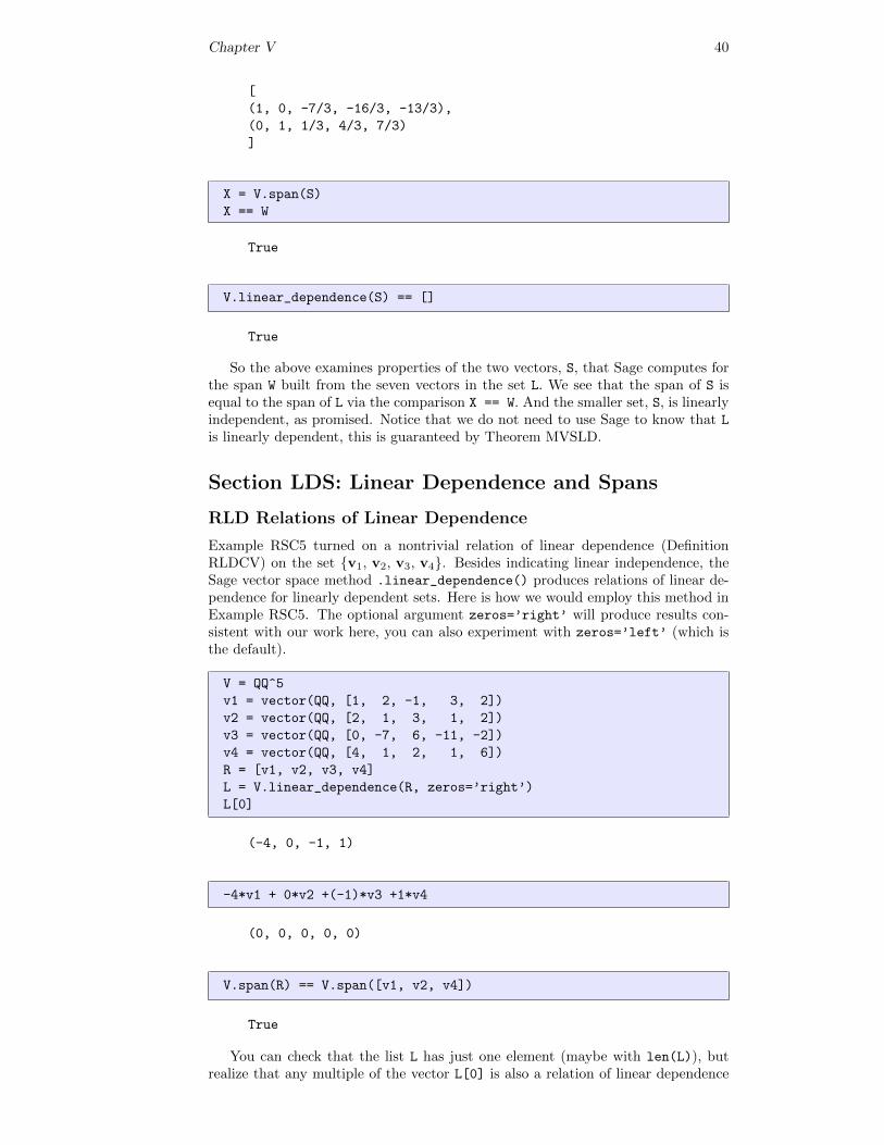
Chapter V 40
[
(1, 0, -7/3, -16/3, -13/3),
(0, 1, 1/3, 4/3, 7/3)
]
X = V.span(S)
X == W
True
V.linear_dependence(S) == []
True
So the above examines properties of the two vectors, S, that Sage computes forthe span W built from the seven vectors in the set L. We see that the span of S isequal to the span of L via the comparison X == W. And the smaller set, S, is linearlyindependent, as promised. Notice that we do not need to use Sage to know that L
is linearly dependent, this is guaranteed by Theorem MVSLD.
Section LDS: Linear Dependence and Spans
RLD Relations of Linear Dependence
Example RSC5 turned on a nontrivial relation of linear dependence (DefinitionRLDCV) on the set {v1, v2, v3, v4}. Besides indicating linear independence, theSage vector space method .linear_dependence() produces relations of linear de-pendence for linearly dependent sets. Here is how we would employ this method inExample RSC5. The optional argument zeros=’right’ will produce results con-sistent with our work here, you can also experiment with zeros=’left’ (which isthe default).
V = QQ^5
v1 = vector(QQ, [1, 2, -1, 3, 2])
v2 = vector(QQ, [2, 1, 3, 1, 2])
v3 = vector(QQ, [0, -7, 6, -11, -2])
v4 = vector(QQ, [4, 1, 2, 1, 6])
R = [v1, v2, v3, v4]
L = V.linear_dependence(R, zeros=’right’)
L[0]
(-4, 0, -1, 1)
-4*v1 + 0*v2 +(-1)*v3 +1*v4
(0, 0, 0, 0, 0)
V.span(R) == V.span([v1, v2, v4])
True
You can check that the list L has just one element (maybe with len(L)), butrealize that any multiple of the vector L[0] is also a relation of linear dependence
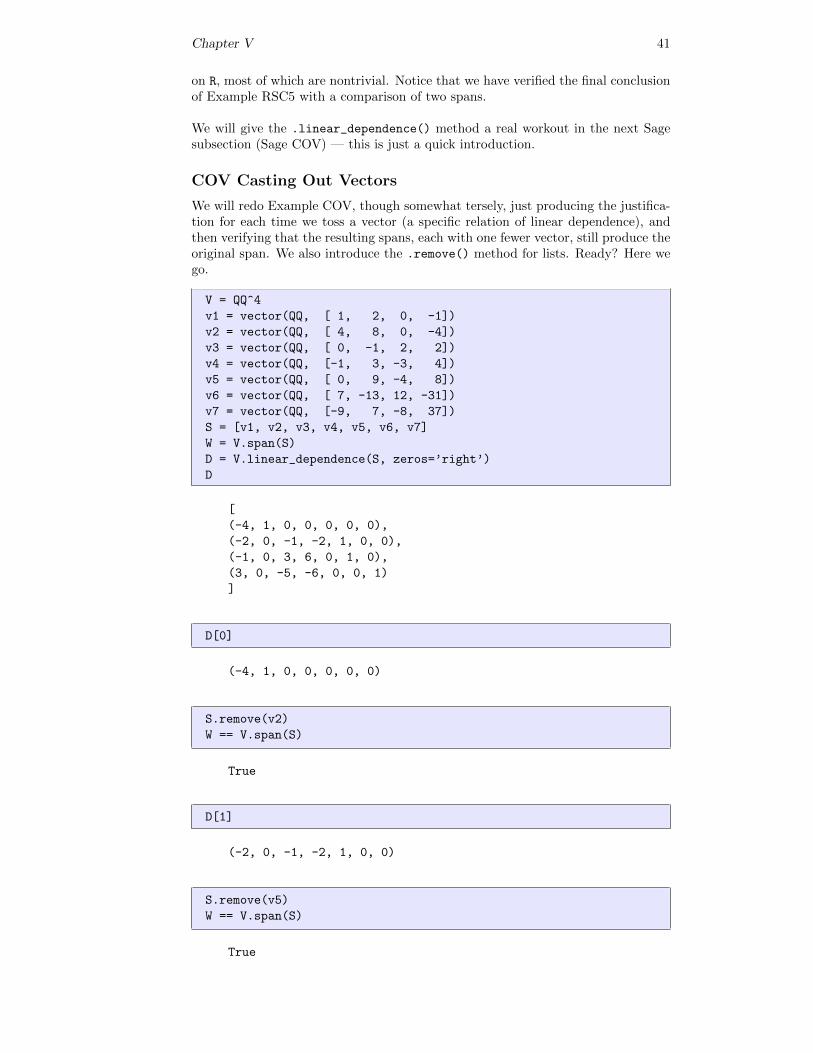
Chapter V 41
on R, most of which are nontrivial. Notice that we have verified the final conclusionof Example RSC5 with a comparison of two spans.
We will give the .linear_dependence() method a real workout in the next Sagesubsection (Sage COV) — this is just a quick introduction.
COV Casting Out Vectors
We will redo Example COV, though somewhat tersely, just producing the justifica-tion for each time we toss a vector (a specific relation of linear dependence), andthen verifying that the resulting spans, each with one fewer vector, still produce theoriginal span. We also introduce the .remove() method for lists. Ready? Here wego.
V = QQ^4
v1 = vector(QQ, [ 1, 2, 0, -1])
v2 = vector(QQ, [ 4, 8, 0, -4])
v3 = vector(QQ, [ 0, -1, 2, 2])
v4 = vector(QQ, [-1, 3, -3, 4])
v5 = vector(QQ, [ 0, 9, -4, 8])
v6 = vector(QQ, [ 7, -13, 12, -31])
v7 = vector(QQ, [-9, 7, -8, 37])
S = [v1, v2, v3, v4, v5, v6, v7]
W = V.span(S)
D = V.linear_dependence(S, zeros=’right’)
D
[
(-4, 1, 0, 0, 0, 0, 0),
(-2, 0, -1, -2, 1, 0, 0),
(-1, 0, 3, 6, 0, 1, 0),
(3, 0, -5, -6, 0, 0, 1)
]
D[0]
(-4, 1, 0, 0, 0, 0, 0)
S.remove(v2)
W == V.span(S)
True
D[1]
(-2, 0, -1, -2, 1, 0, 0)
S.remove(v5)
W == V.span(S)
True
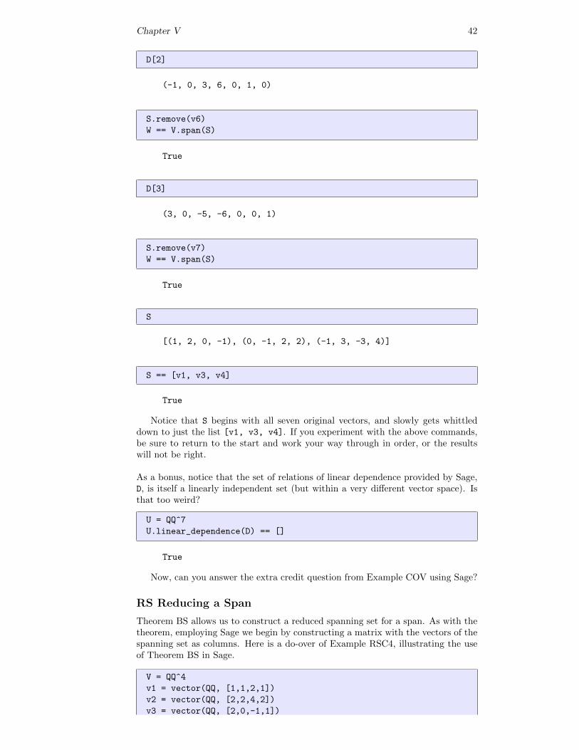
Chapter V 42
D[2]
(-1, 0, 3, 6, 0, 1, 0)
S.remove(v6)
W == V.span(S)
True
D[3]
(3, 0, -5, -6, 0, 0, 1)
S.remove(v7)
W == V.span(S)
True
S
[(1, 2, 0, -1), (0, -1, 2, 2), (-1, 3, -3, 4)]
S == [v1, v3, v4]
True
Notice that S begins with all seven original vectors, and slowly gets whittleddown to just the list [v1, v3, v4]. If you experiment with the above commands,be sure to return to the start and work your way through in order, or the resultswill not be right.
As a bonus, notice that the set of relations of linear dependence provided by Sage,D, is itself a linearly independent set (but within a very different vector space). Isthat too weird?
U = QQ^7
U.linear_dependence(D) == []
True
Now, can you answer the extra credit question from Example COV using Sage?
RS Reducing a Span
Theorem BS allows us to construct a reduced spanning set for a span. As with thetheorem, employing Sage we begin by constructing a matrix with the vectors of thespanning set as columns. Here is a do-over of Example RSC4, illustrating the useof Theorem BS in Sage.
V = QQ^4
v1 = vector(QQ, [1,1,2,1])
v2 = vector(QQ, [2,2,4,2])
v3 = vector(QQ, [2,0,-1,1])
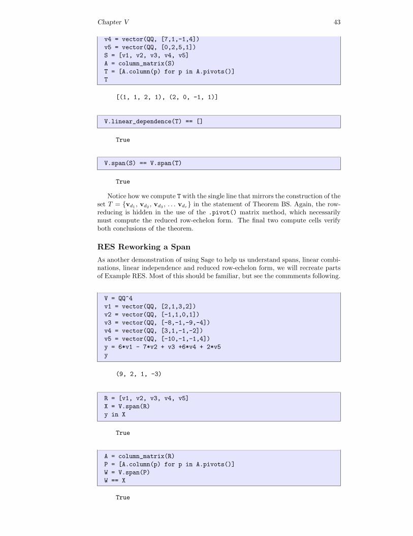
Chapter V 43
v4 = vector(QQ, [7,1,-1,4])
v5 = vector(QQ, [0,2,5,1])
S = [v1, v2, v3, v4, v5]
A = column_matrix(S)
T = [A.column(p) for p in A.pivots()]
T
[(1, 1, 2, 1), (2, 0, -1, 1)]
V.linear_dependence(T) == []
True
V.span(S) == V.span(T)
True
Notice how we compute T with the single line that mirrors the construction of theset T = {vd1 , vd2 , vd3 , . . . vdr} in the statement of Theorem BS. Again, the row-reducing is hidden in the use of the .pivot() matrix method, which necessarilymust compute the reduced row-echelon form. The final two compute cells verifyboth conclusions of the theorem.
RES Reworking a Span
As another demonstration of using Sage to help us understand spans, linear combi-nations, linear independence and reduced row-echelon form, we will recreate partsof Example RES. Most of this should be familiar, but see the commments following.
V = QQ^4
v1 = vector(QQ, [2,1,3,2])
v2 = vector(QQ, [-1,1,0,1])
v3 = vector(QQ, [-8,-1,-9,-4])
v4 = vector(QQ, [3,1,-1,-2])
v5 = vector(QQ, [-10,-1,-1,4])
y = 6*v1 - 7*v2 + v3 +6*v4 + 2*v5
y
(9, 2, 1, -3)
R = [v1, v2, v3, v4, v5]
X = V.span(R)
y in X
True
A = column_matrix(R)
P = [A.column(p) for p in A.pivots()]
W = V.span(P)
W == X
True
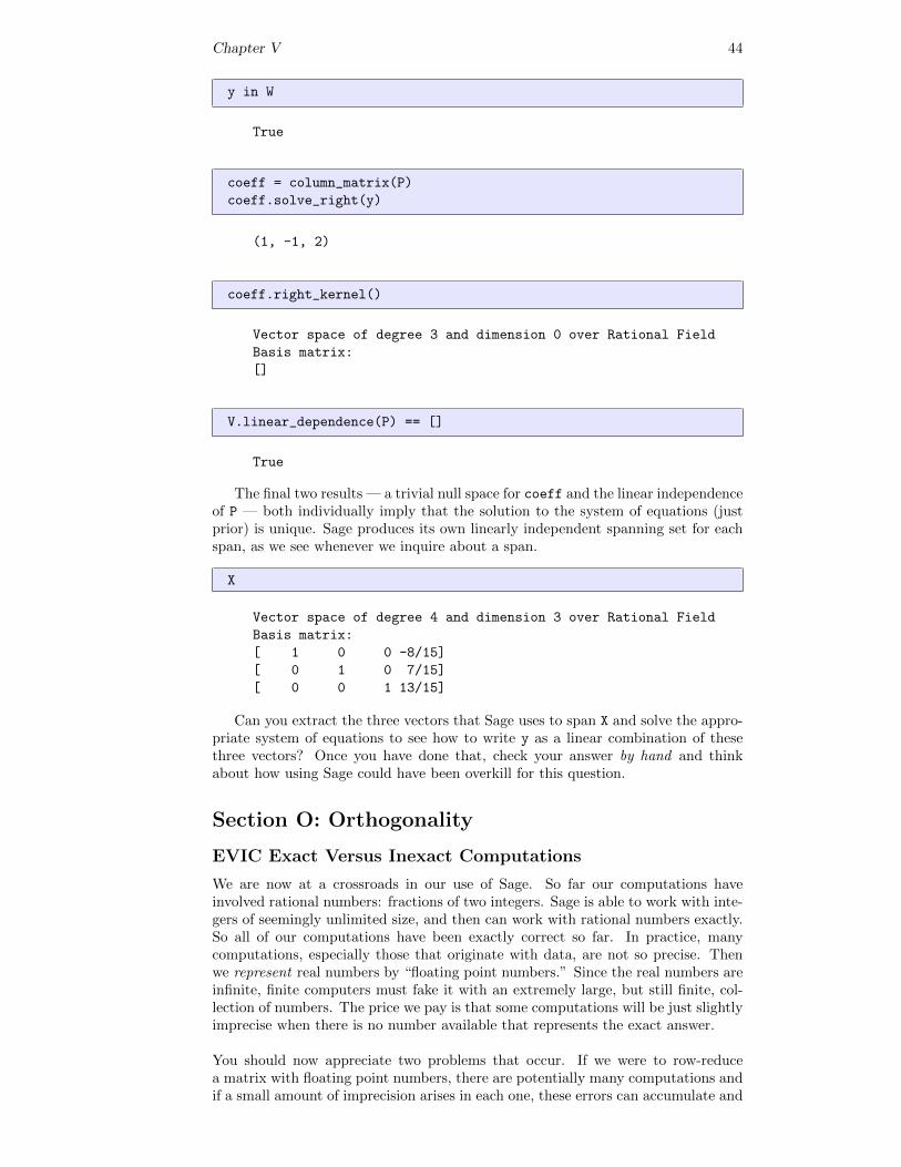
Chapter V 44
y in W
True
coeff = column_matrix(P)
coeff.solve_right(y)
(1, -1, 2)
coeff.right_kernel()
Vector space of degree 3 and dimension 0 over Rational Field
Basis matrix:
[]
V.linear_dependence(P) == []
True
The final two results — a trivial null space for coeff and the linear independenceof P — both individually imply that the solution to the system of equations (justprior) is unique. Sage produces its own linearly independent spanning set for eachspan, as we see whenever we inquire about a span.
X
Vector space of degree 4 and dimension 3 over Rational Field
Basis matrix:
[ 1 0 0 -8/15]
[ 0 1 0 7/15]
[ 0 0 1 13/15]
Can you extract the three vectors that Sage uses to span X and solve the appro-priate system of equations to see how to write y as a linear combination of thesethree vectors? Once you have done that, check your answer by hand and thinkabout how using Sage could have been overkill for this question.
Section O: Orthogonality
EVIC Exact Versus Inexact Computations
We are now at a crossroads in our use of Sage. So far our computations haveinvolved rational numbers: fractions of two integers. Sage is able to work with inte-gers of seemingly unlimited size, and then can work with rational numbers exactly.So all of our computations have been exactly correct so far. In practice, manycomputations, especially those that originate with data, are not so precise. Thenwe represent real numbers by “floating point numbers.” Since the real numbers areinfinite, finite computers must fake it with an extremely large, but still finite, col-lection of numbers. The price we pay is that some computations will be just slightlyimprecise when there is no number available that represents the exact answer.
You should now appreciate two problems that occur. If we were to row-reducea matrix with floating point numbers, there are potentially many computations andif a small amount of imprecision arises in each one, these errors can accumulate and
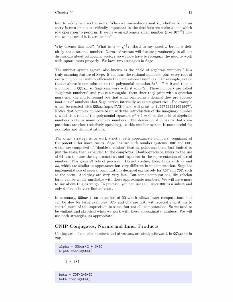
Chapter V 45
lead to wildly incorrect answers. When we row-reduce a matrix, whether or not anentry is zero or not is critically important in the decisions we make about whichrow operation to perform. If we have an extremely small number (like 10−16) howcan we be sure if it is zero or not?
Why discuss this now? What is α =√
73? Hard to say exactly, but it is defi-
nitely not a rational number. Norms of vectors will feature prominently in all ourdiscussions about orthogonal vectors, so we now have to recognize the need to workwith square roots properly. We have two strategies in Sage.
The number system QQbar, also known as the “field of algebraic numbers,” is atruly amazing feature of Sage. It contains the rational numbers, plus every root ofevery polynomial with coefficients that are rational numbers. For example, noticethat α above is one solution to the polynomial equation 3x2 − 7 = 0 and thus isa number in QQbar, so Sage can work with it exactly. These numbers are called“algebraic numbers” and you can recognize them since they print with a questionmark near the end to remind you that when printed as a decimal they are approx-imations of numbers that Sage carries internally as exact quantities. For exampleα can be created with QQbar(sqrt(7/3)) and will print as 1.527525231651947?.Notice that complex numbers begin with the introduction of the imaginary numberi, which is a root of the polynomial equation x2 + 1 = 0, so the field of algebraicnumbers contains many complex numbers. The downside of QQbar is that com-putations are slow (relatively speaking), so this number system is most useful forexamples and demonstrations.
The other strategy is to work strictly with approximate numbers, cognizant ofthe potential for inaccuracies. Sage has two such number systems: RDF and CDF,which are comprised of “double precision” floating point numbers, first limited tojust the reals, then expanded to the complexes. Double-precision refers to the useof 64 bits to store the sign, mantissa and exponent in the representation of a realnumber. This gives 53 bits of precision. Do not confuse these fields with RR andCC, which are similar in appearance but very different in implementation. Sage hasimplementations of several computations designed exclusively for RDF and CDF, suchas the norm. And they are very, very fast. But some computations, like echelonform, can be wildly unreliable with these approximate numbers. We will have moreto say about this as we go. In practice, you can use CDF, since RDF is a subset andonly different in very limited cases.
In summary, QQbar is an extension of QQ which allows exact computations, butcan be slow for large examples. RDF and CDF are fast, with special algorithms tocontrol much of the imprecision in some, but not all, computations. So we need tobe vigilant and skeptical when we work with these approximate numbers. We willuse both strategies, as appropriate.
CNIP Conjugates, Norms and Inner Products
Conjugates, of complex numbers and of vectors, are straightforward, in QQbar or inCDF.
alpha = QQbar(2 + 3*I)
alpha.conjugate()
2 - 3*I
beta = CDF(2+3*I)
beta.conjugate()
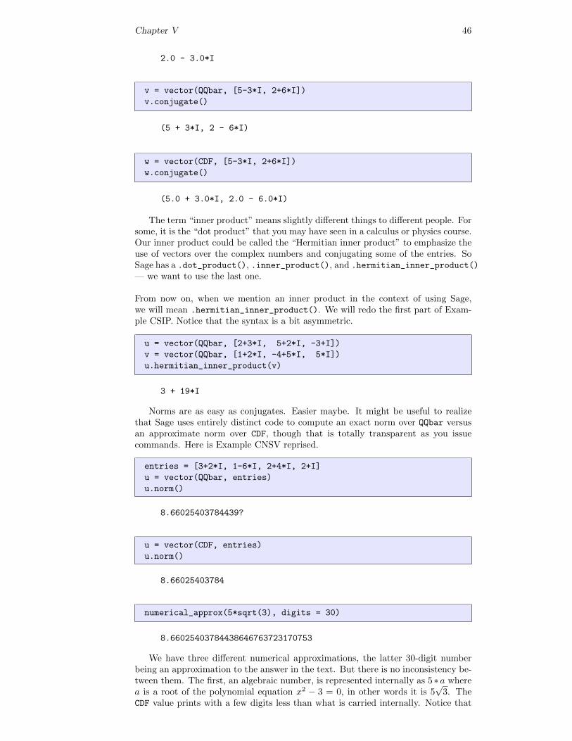
Chapter V 46
2.0 - 3.0*I
v = vector(QQbar, [5-3*I, 2+6*I])
v.conjugate()
(5 + 3*I, 2 - 6*I)
w = vector(CDF, [5-3*I, 2+6*I])
w.conjugate()
(5.0 + 3.0*I, 2.0 - 6.0*I)
The term “inner product” means slightly different things to different people. Forsome, it is the “dot product” that you may have seen in a calculus or physics course.Our inner product could be called the “Hermitian inner product” to emphasize theuse of vectors over the complex numbers and conjugating some of the entries. SoSage has a .dot_product(), .inner_product(), and .hermitian_inner_product()
— we want to use the last one.
From now on, when we mention an inner product in the context of using Sage,we will mean .hermitian_inner_product(). We will redo the first part of Exam-ple CSIP. Notice that the syntax is a bit asymmetric.
u = vector(QQbar, [2+3*I, 5+2*I, -3+I])
v = vector(QQbar, [1+2*I, -4+5*I, 5*I])
u.hermitian_inner_product(v)
3 + 19*I
Norms are as easy as conjugates. Easier maybe. It might be useful to realizethat Sage uses entirely distinct code to compute an exact norm over QQbar versusan approximate norm over CDF, though that is totally transparent as you issuecommands. Here is Example CNSV reprised.
entries = [3+2*I, 1-6*I, 2+4*I, 2+I]
u = vector(QQbar, entries)
u.norm()
8.66025403784439?
u = vector(CDF, entries)
u.norm()
8.66025403784
numerical_approx(5*sqrt(3), digits = 30)
8.66025403784438646763723170753
We have three different numerical approximations, the latter 30-digit numberbeing an approximation to the answer in the text. But there is no inconsistency be-tween them. The first, an algebraic number, is represented internally as 5 ∗a wherea is a root of the polynomial equation x2 − 3 = 0, in other words it is 5
√3. The
CDF value prints with a few digits less than what is carried internally. Notice that
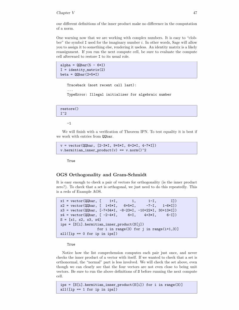
Chapter V 47
our different definitions of the inner product make no difference in the computationof a norm.
One warning now that we are working with complex numbers. It is easy to “clob-ber” the symbol I used for the imaginary number i. In other words, Sage will allowyou to assign it to something else, rendering it useless. An identity matrix is a likelyreassignment. If you run the next compute cell, be sure to evaluate the computecell afterward to restore I to its usual role.
alpha = QQbar(5 - 6*I)
I = identity_matrix(2)
beta = QQbar(2+5*I)
Traceback (most recent call last):
...
TypeError: Illegal initializer for algebraic number
restore()
I^2
-1
We will finish with a verification of Theorem IPN. To test equality it is best ifwe work with entries from QQbar.
v = vector(QQbar, [2-3*I, 9+5*I, 6+2*I, 4-7*I])
v.hermitian_inner_product(v) == v.norm()^2
True
OGS Orthogonality and Gram-Schmidt
It is easy enough to check a pair of vectors for orthogonality (is the inner productzero?). To check that a set is orthogonal, we just need to do this repeatedly. Thisis a redo of Example AOS.
x1 = vector(QQbar, [ 1+I, 1, 1-I, I])
x2 = vector(QQbar, [ 1+5*I, 6+5*I, -7-I, 1-6*I])
x3 = vector(QQbar, [-7+34*I, -8-23*I, -10+22*I, 30+13*I])
x4 = vector(QQbar, [ -2-4*I, 6+I, 4+3*I, 6-I])
S = [x1, x2, x3, x4]
ips = [S[i].hermitian_inner_product(S[j])
for i in range(3) for j in range(i+1,3)]
all([ip == 0 for ip in ips])
True
Notice how the list comprehension computes each pair just once, and neverchecks the inner product of a vector with itself. If we wanted to check that a set isorthonormal, the “normal” part is less involved. We will check the set above, eventhough we can clearly see that the four vectors are not even close to being unitvectors. Be sure to run the above definitions of S before running the next computecell.
ips = [S[i].hermitian_inner_product(S[i]) for i in range(3)]
all([ip == 1 for ip in ips])
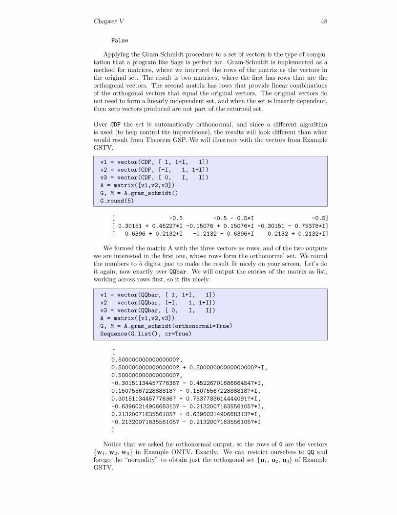
Chapter V 48
False
Applying the Gram-Schmidt procedure to a set of vectors is the type of compu-tation that a program like Sage is perfect for. Gram-Schmidt is implemented as amethod for matrices, where we interpret the rows of the matrix as the vectors inthe original set. The result is two matrices, where the first has rows that are theorthogonal vectors. The second matrix has rows that provide linear combinationsof the orthogonal vectors that equal the original vectors. The original vectors donot need to form a linearly independent set, and when the set is linearly dependent,then zero vectors produced are not part of the returned set.
Over CDF the set is automatically orthonormal, and since a different algorithmis used (to help control the imprecisions), the results will look different than whatwould result from Theorem GSP. We will illustrate with the vectors from ExampleGSTV.
v1 = vector(CDF, [ 1, 1+I, 1])
v2 = vector(CDF, [-I, 1, 1+I])
v3 = vector(CDF, [ 0, I, I])
A = matrix([v1,v2,v3])
G, M = A.gram_schmidt()
G.round(5)
[ -0.5 -0.5 - 0.5*I -0.5]
[ 0.30151 + 0.45227*I -0.15076 + 0.15076*I -0.30151 - 0.75378*I]
[ 0.6396 + 0.2132*I -0.2132 - 0.6396*I 0.2132 + 0.2132*I]
We formed the matrix A with the three vectors as rows, and of the two outputswe are interested in the first one, whose rows form the orthonormal set. We roundthe numbers to 5 digits, just to make the result fit nicely on your screen. Let’s doit again, now exactly over QQbar. We will output the entries of the matrix as list,working across rows first, so it fits nicely.
v1 = vector(QQbar, [ 1, 1+I, 1])
v2 = vector(QQbar, [-I, 1, 1+I])
v3 = vector(QQbar, [ 0, I, I])
A = matrix([v1,v2,v3])
G, M = A.gram_schmidt(orthonormal=True)
Sequence(G.list(), cr=True)
[
0.50000000000000000?,
0.50000000000000000? + 0.50000000000000000?*I,
0.50000000000000000?,
-0.3015113445777636? - 0.4522670168666454?*I,
0.1507556722888818? - 0.1507556722888818?*I,
0.3015113445777636? + 0.7537783614444091?*I,
-0.6396021490668313? - 0.2132007163556105?*I,
0.2132007163556105? + 0.6396021490668313?*I,
-0.2132007163556105? - 0.2132007163556105?*I
]
Notice that we asked for orthonormal output, so the rows of G are the vectors{w1, w2, w3} in Example ONTV. Exactly. We can restrict ourselves to QQ andforego the “normality” to obtain just the orthogonal set {u1, u2, u3} of ExampleGSTV.
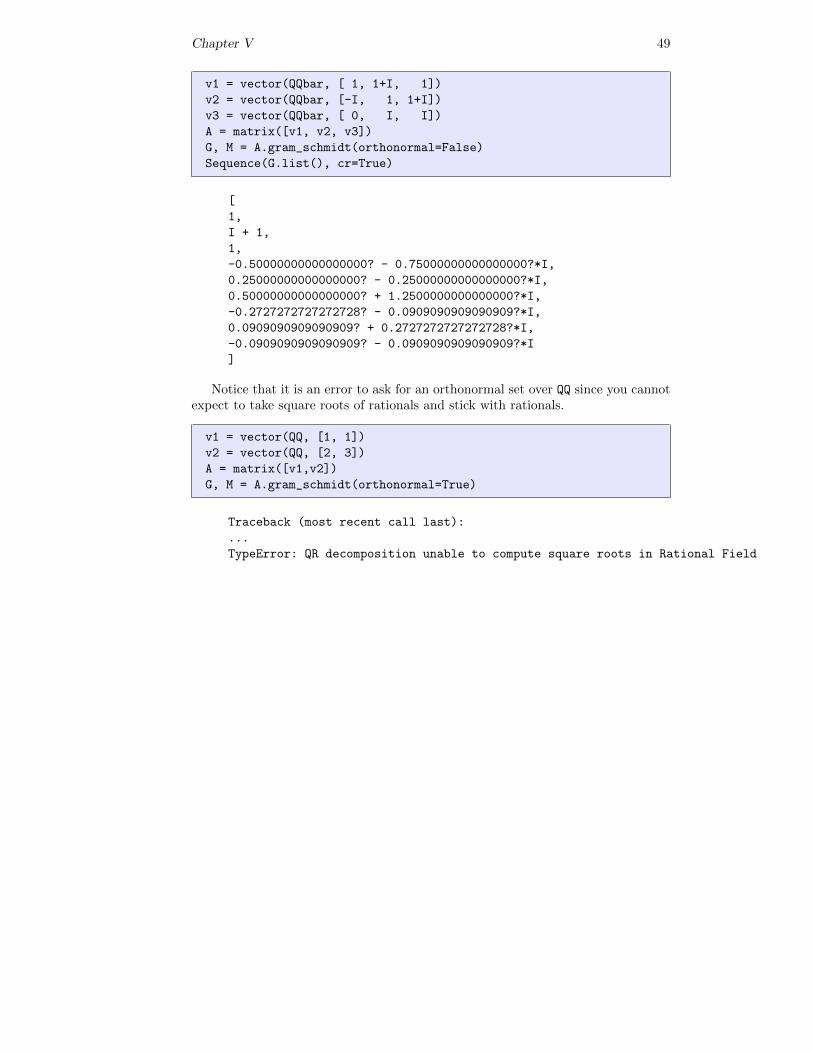
Chapter V 49
v1 = vector(QQbar, [ 1, 1+I, 1])
v2 = vector(QQbar, [-I, 1, 1+I])
v3 = vector(QQbar, [ 0, I, I])
A = matrix([v1, v2, v3])
G, M = A.gram_schmidt(orthonormal=False)
Sequence(G.list(), cr=True)
[
1,
I + 1,
1,
-0.50000000000000000? - 0.75000000000000000?*I,
0.25000000000000000? - 0.25000000000000000?*I,
0.50000000000000000? + 1.2500000000000000?*I,
-0.2727272727272728? - 0.0909090909090909?*I,
0.0909090909090909? + 0.2727272727272728?*I,
-0.0909090909090909? - 0.0909090909090909?*I
]
Notice that it is an error to ask for an orthonormal set over QQ since you cannotexpect to take square roots of rationals and stick with rationals.
v1 = vector(QQ, [1, 1])
v2 = vector(QQ, [2, 3])
A = matrix([v1,v2])
G, M = A.gram_schmidt(orthonormal=True)
Traceback (most recent call last):
...
TypeError: QR decomposition unable to compute square roots in Rational Field
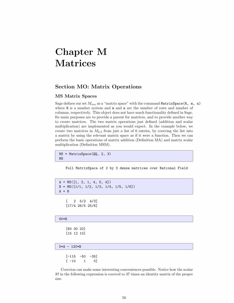
Chapter MMatrices
Section MO: Matrix Operations
MS Matrix Spaces
Sage defines our setMmn as a “matrix space” with the command MatrixSpace(R, m, n)
where R is a number system and m and n are the number of rows and number ofcolumns, respectively. This object does not have much functionality defined in Sage.Its main purposes are to provide a parent for matrices, and to provide another wayto create matrices. The two matrix operations just defined (addition and scalarmultiplication) are implemented as you would expect. In the example below, wecreate two matrices in M2,3 from just a list of 6 entries, by coercing the list intoa matrix by using the relevant matrix space as if it were a function. Then we canperform the basic operations of matrix addition (Definition MA) and matrix scalarmultiplication (Definition MSM).
MS = MatrixSpace(QQ, 2, 3)
MS
Full MatrixSpace of 2 by 3 dense matrices over Rational Field
A = MS([1, 2, 1, 4, 5, 4])
B = MS([1/1, 1/2, 1/3, 1/4, 1/5, 1/6])
A + B
[ 2 5/2 4/3]
[17/4 26/5 25/6]
60*B
[60 30 20]
[15 12 10]
5*A - 120*B
[-115 -50 -35]
[ -10 1 0]
Coercion can make some interesting conveniences possible. Notice how the scalar37 in the following expression is coerced to 37 times an identity matrix of the propersize.
50
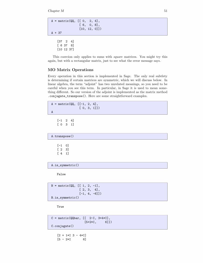
Chapter M 51
A = matrix(QQ, [[ 0, 2, 4],
[ 6, 0, 8],
[10, 12, 0]])
A + 37
[37 2 4]
[ 6 37 8]
[10 12 37]
This coercion only applies to sums with square matrices. You might try thisagain, but with a rectangular matrix, just to see what the error message says.
MO Matrix Operations
Every operation in this section is implemented in Sage. The only real subtletyis determining if certain matrices are symmetric, which we will discuss below. Inlinear algebra, the term “adjoint” has two unrelated meanings, so you need to becareful when you see this term. In particular, in Sage it is used to mean some-thing different. So our version of the adjoint is implemented as the matrix method.conjugate_transpose(). Here are some straightforward examples.
A = matrix(QQ, [[-1, 2, 4],
[ 0, 3, 1]])
A
[-1 2 4]
[ 0 3 1]
A.transpose()
[-1 0]
[ 2 3]
[ 4 1]
A.is_symmetric()
False
B = matrix(QQ, [[ 1, 2, -1],
[ 2, 3, 4],
[-1, 4, -6]])
B.is_symmetric()
True
C = matrix(QQbar, [[ 2-I, 3+4*I],
[5+2*I, 6]])
C.conjugate()
[2 + 1*I 3 - 4*I]
[5 - 2*I 6]
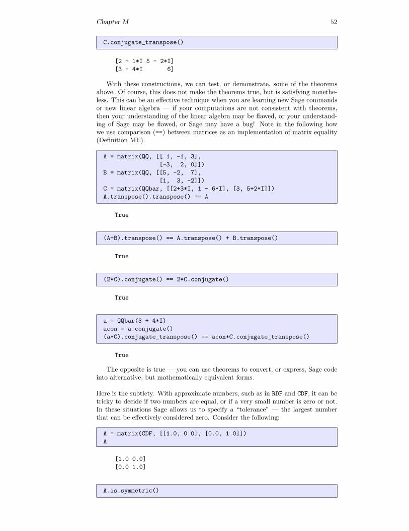
Chapter M 52
C.conjugate_transpose()
[2 + 1*I 5 - 2*I]
[3 - 4*I 6]
With these constructions, we can test, or demonstrate, some of the theoremsabove. Of course, this does not make the theorems true, but is satisfying nonethe-less. This can be an effective technique when you are learning new Sage commandsor new linear algebra — if your computations are not consistent with theorems,then your understanding of the linear algebra may be flawed, or your understand-ing of Sage may be flawed, or Sage may have a bug! Note in the following howwe use comparison (==) between matrices as an implementation of matrix equality(Definition ME).
A = matrix(QQ, [[ 1, -1, 3],
[-3, 2, 0]])
B = matrix(QQ, [[5, -2, 7],
[1, 3, -2]])
C = matrix(QQbar, [[2+3*I, 1 - 6*I], [3, 5+2*I]])
A.transpose().transpose() == A
True
(A+B).transpose() == A.transpose() + B.transpose()
True
(2*C).conjugate() == 2*C.conjugate()
True
a = QQbar(3 + 4*I)
acon = a.conjugate()
(a*C).conjugate_transpose() == acon*C.conjugate_transpose()
True
The opposite is true — you can use theorems to convert, or express, Sage codeinto alternative, but mathematically equivalent forms.
Here is the subtlety. With approximate numbers, such as in RDF and CDF, it can betricky to decide if two numbers are equal, or if a very small number is zero or not.In these situations Sage allows us to specify a “tolerance” — the largest numberthat can be effectively considered zero. Consider the following:
A = matrix(CDF, [[1.0, 0.0], [0.0, 1.0]])
A
[1.0 0.0]
[0.0 1.0]
A.is_symmetric()
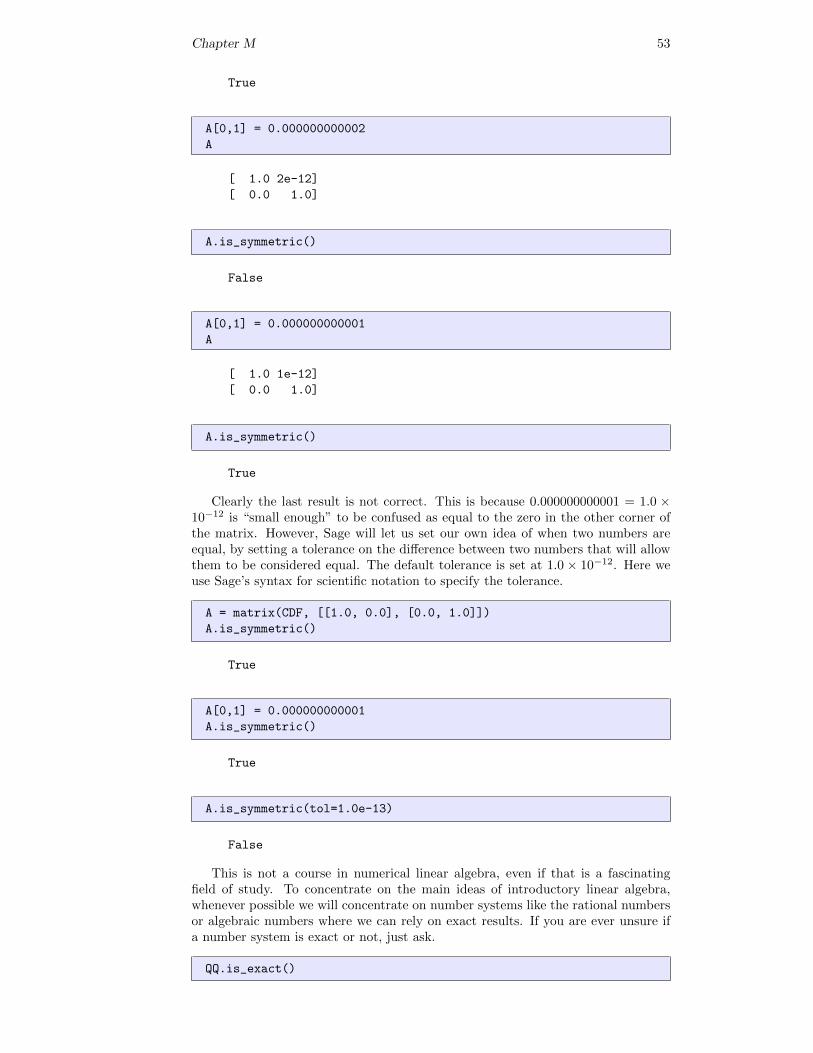
Chapter M 53
True
A[0,1] = 0.000000000002
A
[ 1.0 2e-12]
[ 0.0 1.0]
A.is_symmetric()
False
A[0,1] = 0.000000000001
A
[ 1.0 1e-12]
[ 0.0 1.0]
A.is_symmetric()
True
Clearly the last result is not correct. This is because 0.000000000001 = 1.0 ×10⁻¹² is “small enough” to be confused as equal to the zero in the other corner ofthe matrix. However, Sage will let us set our own idea of when two numbers areequal, by setting a tolerance on the difference between two numbers that will allowthem to be considered equal. The default tolerance is set at 1.0 × 10⁻¹². Here weuse Sage’s syntax for scientific notation to specify the tolerance.
A = matrix(CDF, [[1.0, 0.0], [0.0, 1.0]])
A.is_symmetric()
True
A[0,1] = 0.000000000001
A.is_symmetric()
True
A.is_symmetric(tol=1.0e-13)
False
This is not a course in numerical linear algebra, even if that is a fascinatingfield of study. To concentrate on the main ideas of introductory linear algebra,whenever possible we will concentrate on number systems like the rational numbersor algebraic numbers where we can rely on exact results. If you are ever unsure ifa number system is exact or not, just ask.
QQ.is_exact()
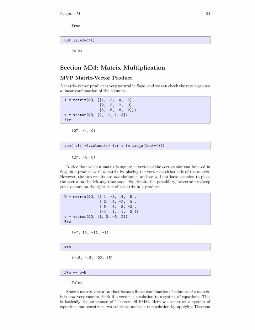
Chapter M 54
True
RDF.is_exact()
False
Section MM: Matrix Multiplication
MVP Matrix-Vector Product
A matrix-vector product is very natural in Sage, and we can check the result againsta linear combination of the columns.
A = matrix(QQ, [[1, -3, 4, 5],
[2, 3, -2, 0],
[5, 6, 8, -2]])
v = vector(QQ, [2, -2, 1, 3])
A*v
(27, -4, 0)
sum([v[i]*A.column(i) for i in range(len(v))])
(27, -4, 0)
Notice that when a matrix is square, a vector of the correct size can be used inSage in a product with a matrix by placing the vector on either side of the matrix.However, the two results are not the same, and we will not have ocassion to placethe vector on the left any time soon. So, despite the possibility, be certain to keepyour vectors on the right side of a matrix in a product.
B = matrix(QQ, [[ 1, -3, 4, 5],
[ 2, 3, -2, 0],
[ 5, 6, 8, -2],
[-4, 1, 1, 2]])
w = vector(QQ, [1, 2, -3, 2])
B*w
(-7, 14, -11, -1)
w*B
(-18, -13, -22, 15)
B*w == w*B
False
Since a matrix-vector product forms a linear combination of columns of a matrix,it is now very easy to check if a vector is a solution to a system of equations. Thisis basically the substance of Theorem SLEMM. Here we construct a system ofequations and construct two solutions and one non-solution by applying Theorem
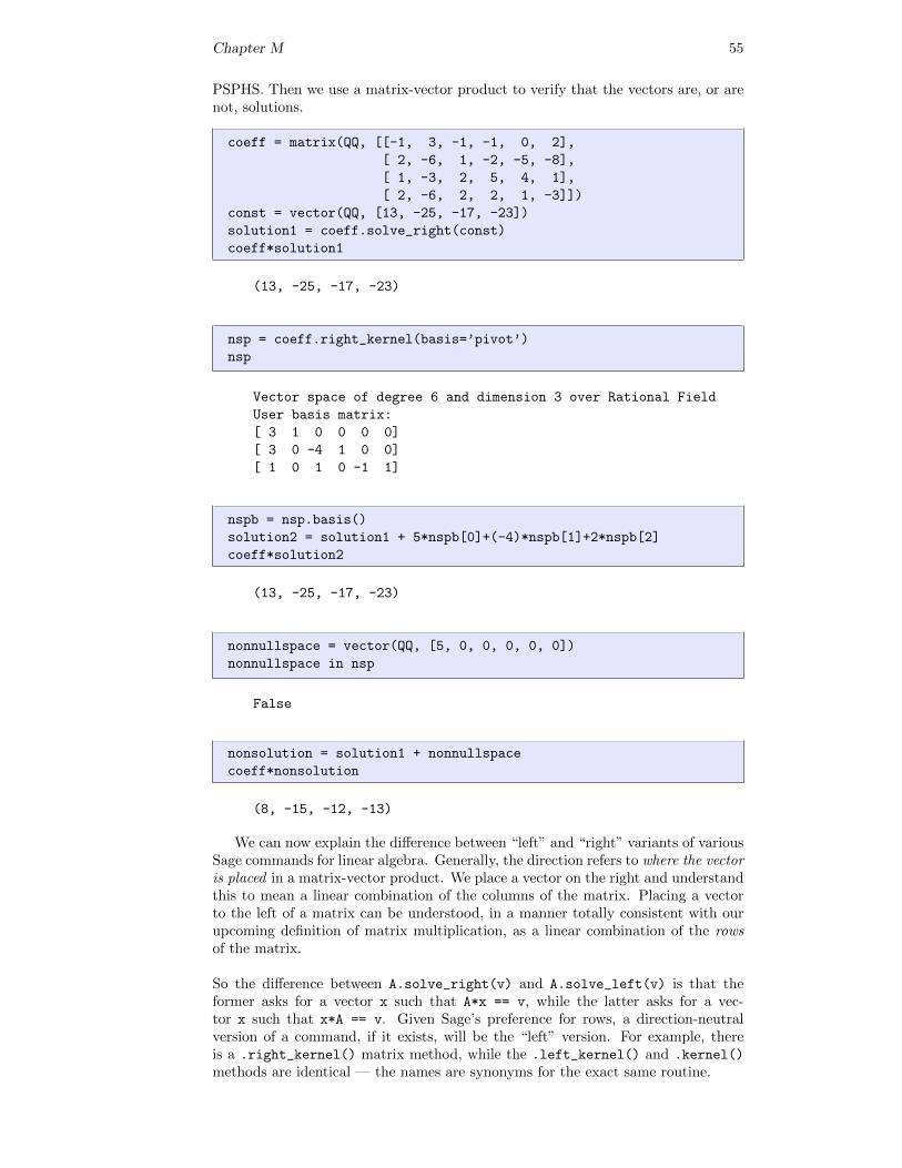
Chapter M 55
PSPHS. Then we use a matrix-vector product to verify that the vectors are, or arenot, solutions.
coeff = matrix(QQ, [[-1, 3, -1, -1, 0, 2],
[ 2, -6, 1, -2, -5, -8],
[ 1, -3, 2, 5, 4, 1],
[ 2, -6, 2, 2, 1, -3]])
const = vector(QQ, [13, -25, -17, -23])
solution1 = coeff.solve_right(const)
coeff*solution1
(13, -25, -17, -23)
nsp = coeff.right_kernel(basis=’pivot’)
nsp
Vector space of degree 6 and dimension 3 over Rational Field
User basis matrix:
[ 3 1 0 0 0 0]
[ 3 0 -4 1 0 0]
[ 1 0 1 0 -1 1]
nspb = nsp.basis()
solution2 = solution1 + 5*nspb[0]+(-4)*nspb[1]+2*nspb[2]
coeff*solution2
(13, -25, -17, -23)
nonnullspace = vector(QQ, [5, 0, 0, 0, 0, 0])
nonnullspace in nsp
False
nonsolution = solution1 + nonnullspace
coeff*nonsolution
(8, -15, -12, -13)
We can now explain the difference between “left” and “right” variants of variousSage commands for linear algebra. Generally, the direction refers to where the vectoris placed in a matrix-vector product. We place a vector on the right and understandthis to mean a linear combination of the columns of the matrix. Placing a vectorto the left of a matrix can be understood, in a manner totally consistent with ourupcoming definition of matrix multiplication, as a linear combination of the rowsof the matrix.
So the difference between A.solve_right(v) and A.solve_left(v) is that theformer asks for a vector x such that A*x == v, while the latter asks for a vec-tor x such that x*A == v. Given Sage’s preference for rows, a direction-neutralversion of a command, if it exists, will be the “left” version. For example, thereis a .right_kernel() matrix method, while the .left_kernel() and .kernel()
methods are identical — the names are synonyms for the exact same routine.
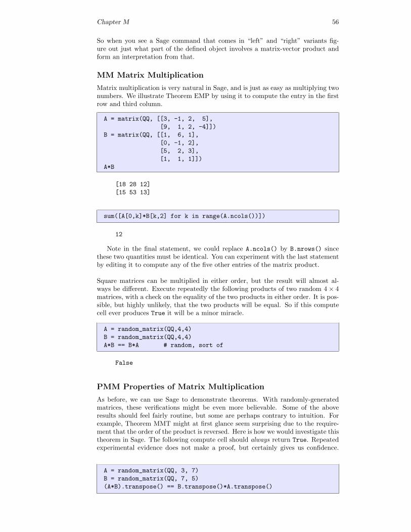
Chapter M 56
So when you see a Sage command that comes in “left” and “right” variants fig-ure out just what part of the defined object involves a matrix-vector product andform an interpretation from that.
MM Matrix Multiplication
Matrix multiplication is very natural in Sage, and is just as easy as multiplying twonumbers. We illustrate Theorem EMP by using it to compute the entry in the firstrow and third column.
A = matrix(QQ, [[3, -1, 2, 5],
[9, 1, 2, -4]])
B = matrix(QQ, [[1, 6, 1],
[0, -1, 2],
[5, 2, 3],
[1, 1, 1]])
A*B
[18 28 12]
[15 53 13]
sum([A[0,k]*B[k,2] for k in range(A.ncols())])
12
Note in the final statement, we could replace A.ncols() by B.nrows() sincethese two quantities must be identical. You can experiment with the last statementby editing it to compute any of the five other entries of the matrix product.
Square matrices can be multiplied in either order, but the result will almost al-ways be different. Execute repeatedly the following products of two random 4 × 4matrices, with a check on the equality of the two products in either order. It is pos-sible, but highly unlikely, that the two products will be equal. So if this computecell ever produces True it will be a minor miracle.
A = random_matrix(QQ,4,4)
B = random_matrix(QQ,4,4)
A*B == B*A # random, sort of
False
PMM Properties of Matrix Multiplication
As before, we can use Sage to demonstrate theorems. With randomly-generatedmatrices, these verifications might be even more believable. Some of the aboveresults should feel fairly routine, but some are perhaps contrary to intuition. Forexample, Theorem MMT might at first glance seem surprising due to the require-ment that the order of the product is reversed. Here is how we would investigate thistheorem in Sage. The following compute cell should always return True. Repeatedexperimental evidence does not make a proof, but certainly gives us confidence.
A = random_matrix(QQ, 3, 7)
B = random_matrix(QQ, 7, 5)
(A*B).transpose() == B.transpose()*A.transpose()
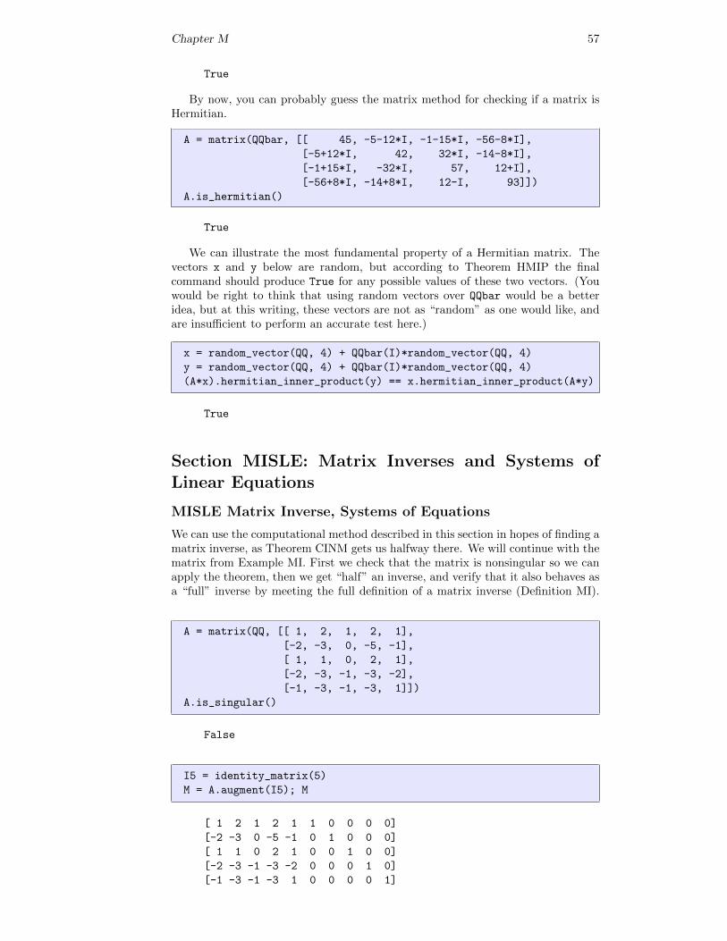
Chapter M 57
True
By now, you can probably guess the matrix method for checking if a matrix isHermitian.
A = matrix(QQbar, [[ 45, -5-12*I, -1-15*I, -56-8*I],
[-5+12*I, 42, 32*I, -14-8*I],
[-1+15*I, -32*I, 57, 12+I],
[-56+8*I, -14+8*I, 12-I, 93]])
A.is_hermitian()
True
We can illustrate the most fundamental property of a Hermitian matrix. Thevectors x and y below are random, but according to Theorem HMIP the finalcommand should produce True for any possible values of these two vectors. (Youwould be right to think that using random vectors over QQbar would be a betteridea, but at this writing, these vectors are not as “random” as one would like, andare insufficient to perform an accurate test here.)
x = random_vector(QQ, 4) + QQbar(I)*random_vector(QQ, 4)
y = random_vector(QQ, 4) + QQbar(I)*random_vector(QQ, 4)
(A*x).hermitian_inner_product(y) == x.hermitian_inner_product(A*y)
True
Section MISLE: Matrix Inverses and Systems ofLinear Equations
MISLE Matrix Inverse, Systems of Equations
We can use the computational method described in this section in hopes of finding amatrix inverse, as Theorem CINM gets us halfway there. We will continue with thematrix from Example MI. First we check that the matrix is nonsingular so we canapply the theorem, then we get “half” an inverse, and verify that it also behaves asa “full” inverse by meeting the full definition of a matrix inverse (Definition MI).
A = matrix(QQ, [[ 1, 2, 1, 2, 1],
[-2, -3, 0, -5, -1],
[ 1, 1, 0, 2, 1],
[-2, -3, -1, -3, -2],
[-1, -3, -1, -3, 1]])
A.is_singular()
False
I5 = identity_matrix(5)
M = A.augment(I5); M
[ 1 2 1 2 1 1 0 0 0 0]
[-2 -3 0 -5 -1 0 1 0 0 0]
[ 1 1 0 2 1 0 0 1 0 0]
[-2 -3 -1 -3 -2 0 0 0 1 0]
[-1 -3 -1 -3 1 0 0 0 0 1]
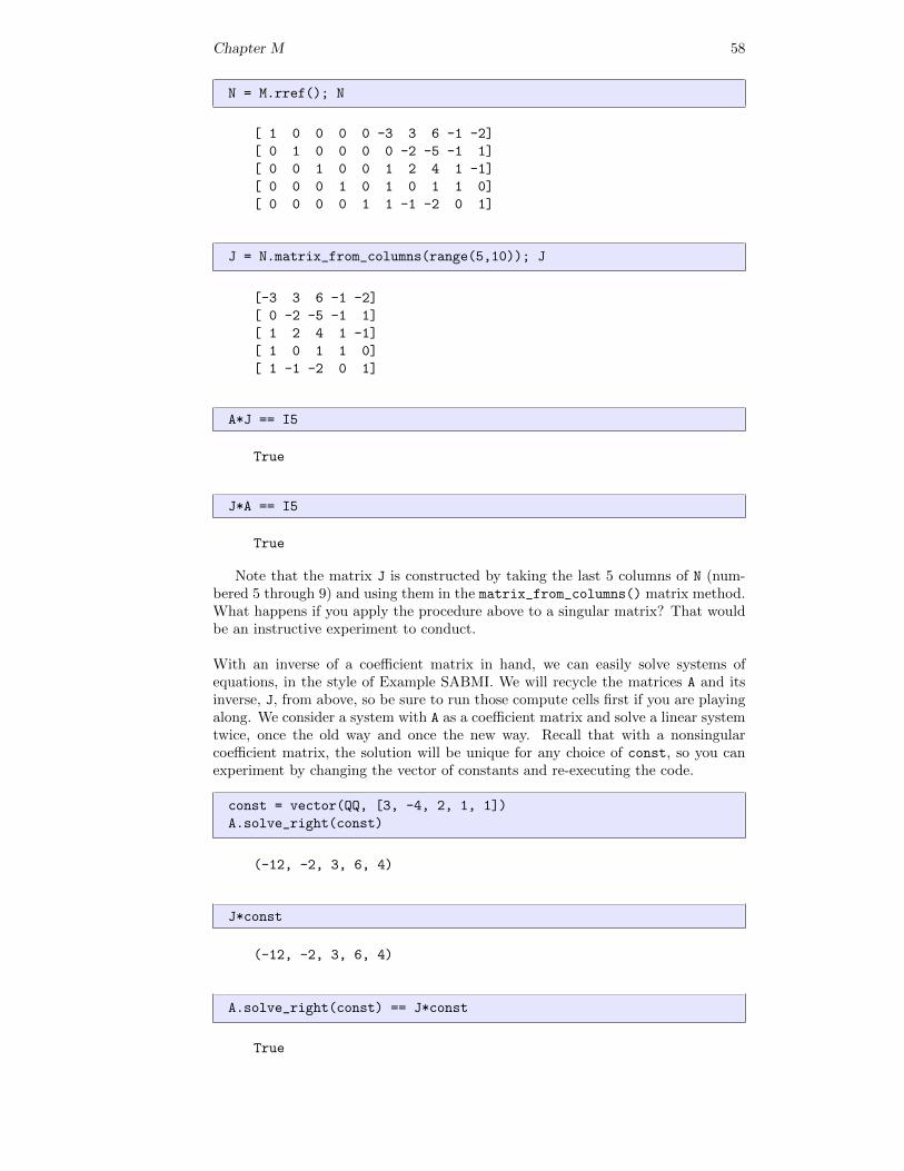
Chapter M 58
N = M.rref(); N
[ 1 0 0 0 0 -3 3 6 -1 -2]
[ 0 1 0 0 0 0 -2 -5 -1 1]
[ 0 0 1 0 0 1 2 4 1 -1]
[ 0 0 0 1 0 1 0 1 1 0]
[ 0 0 0 0 1 1 -1 -2 0 1]
J = N.matrix_from_columns(range(5,10)); J
[-3 3 6 -1 -2]
[ 0 -2 -5 -1 1]
[ 1 2 4 1 -1]
[ 1 0 1 1 0]
[ 1 -1 -2 0 1]
A*J == I5
True
J*A == I5
True
Note that the matrix J is constructed by taking the last 5 columns of N (num-bered 5 through 9) and using them in the matrix_from_columns() matrix method.What happens if you apply the procedure above to a singular matrix? That wouldbe an instructive experiment to conduct.
With an inverse of a coefficient matrix in hand, we can easily solve systems ofequations, in the style of Example SABMI. We will recycle the matrices A and itsinverse, J, from above, so be sure to run those compute cells first if you are playingalong. We consider a system with A as a coefficient matrix and solve a linear systemtwice, once the old way and once the new way. Recall that with a nonsingularcoefficient matrix, the solution will be unique for any choice of const, so you canexperiment by changing the vector of constants and re-executing the code.
const = vector(QQ, [3, -4, 2, 1, 1])
A.solve_right(const)
(-12, -2, 3, 6, 4)
J*const
(-12, -2, 3, 6, 4)
A.solve_right(const) == J*const
True
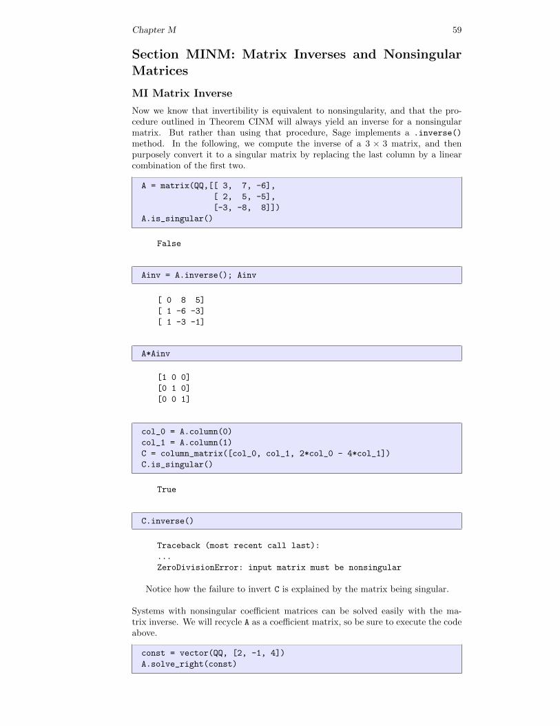
Chapter M 59
Section MINM: Matrix Inverses and NonsingularMatrices
MI Matrix Inverse
Now we know that invertibility is equivalent to nonsingularity, and that the pro-cedure outlined in Theorem CINM will always yield an inverse for a nonsingularmatrix. But rather than using that procedure, Sage implements a .inverse()
method. In the following, we compute the inverse of a 3 × 3 matrix, and thenpurposely convert it to a singular matrix by replacing the last column by a linearcombination of the first two.
A = matrix(QQ,[[ 3, 7, -6],
[ 2, 5, -5],
[-3, -8, 8]])
A.is_singular()
False
Ainv = A.inverse(); Ainv
[ 0 8 5]
[ 1 -6 -3]
[ 1 -3 -1]
A*Ainv
[1 0 0]
[0 1 0]
[0 0 1]
col_0 = A.column(0)
col_1 = A.column(1)
C = column_matrix([col_0, col_1, 2*col_0 - 4*col_1])
C.is_singular()
True
C.inverse()
Traceback (most recent call last):
...
ZeroDivisionError: input matrix must be nonsingular
Notice how the failure to invert C is explained by the matrix being singular.
Systems with nonsingular coefficient matrices can be solved easily with the ma-trix inverse. We will recycle A as a coefficient matrix, so be sure to execute the codeabove.
const = vector(QQ, [2, -1, 4])
A.solve_right(const)
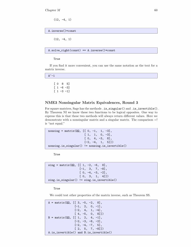
Chapter M 60
(12, -4, 1)
A.inverse()*const
(12, -4, 1)
A.solve_right(const) == A.inverse()*const
True
If you find it more convenient, you can use the same notation as the text for amatrix inverse.
A^-1
[ 0 8 5]
[ 1 -6 -3]
[ 1 -3 -1]
NME3 Nonsingular Matrix Equivalences, Round 3
For square matrices, Sage has the methods .is_singular() and .is_invertible().By Theorem NI we know these two functions to be logical opposites. One way toexpress this is that these two methods will always return different values. Here wedemonstrate with a nonsingular matrix and a singular matrix. The comparison =!is “not equal.”
nonsing = matrix(QQ, [[ 0, -1, 1, -3],
[ 1, 1, 0, -3],
[ 0, 4, -3, 8],
[-2, -4, 1, 5]])
nonsing.is_singular() != nonsing.is_invertible()
True
sing = matrix(QQ, [[ 1, -2, -6, 8],
[-1, 3, 7, -8],
[ 0, -4, -3, -2],
[ 0, 3, 1, 4]])
sing.is_singular() != sing.is_invertible()
True
We could test other properties of the matrix inverse, such as Theorem SS.
A = matrix(QQ, [[ 3, -5, -2, 8],
[-1, 2, 0, -1],
[-2, 4, 1, -4],
[ 4, -5, 0, 8]])
B = matrix(QQ, [[ 1, 2, 4, -1],
[-2, -3, -8, -2],
[-2, -4, -7, 5],
[ 2, 5, 7, -8]])
A.is_invertible() and B.is_invertible()
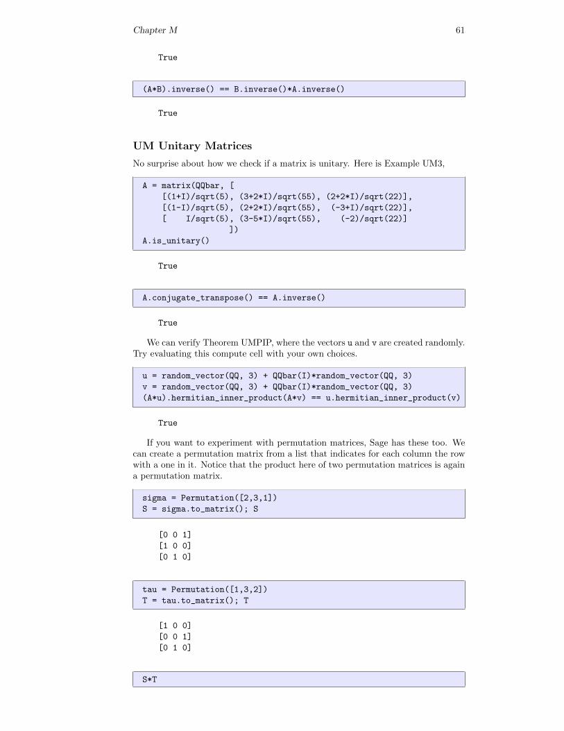
Chapter M 61
True
(A*B).inverse() == B.inverse()*A.inverse()
True
UM Unitary Matrices
No surprise about how we check if a matrix is unitary. Here is Example UM3,
A = matrix(QQbar, [
[(1+I)/sqrt(5), (3+2*I)/sqrt(55), (2+2*I)/sqrt(22)],
[(1-I)/sqrt(5), (2+2*I)/sqrt(55), (-3+I)/sqrt(22)],
[ I/sqrt(5), (3-5*I)/sqrt(55), (-2)/sqrt(22)]
])
A.is_unitary()
True
A.conjugate_transpose() == A.inverse()
True
We can verify Theorem UMPIP, where the vectors u and v are created randomly.Try evaluating this compute cell with your own choices.
u = random_vector(QQ, 3) + QQbar(I)*random_vector(QQ, 3)
v = random_vector(QQ, 3) + QQbar(I)*random_vector(QQ, 3)
(A*u).hermitian_inner_product(A*v) == u.hermitian_inner_product(v)
True
If you want to experiment with permutation matrices, Sage has these too. Wecan create a permutation matrix from a list that indicates for each column the rowwith a one in it. Notice that the product here of two permutation matrices is againa permutation matrix.
sigma = Permutation([2,3,1])
S = sigma.to_matrix(); S
[0 0 1]
[1 0 0]
[0 1 0]
tau = Permutation([1,3,2])
T = tau.to_matrix(); T
[1 0 0]
[0 0 1]
[0 1 0]
S*T
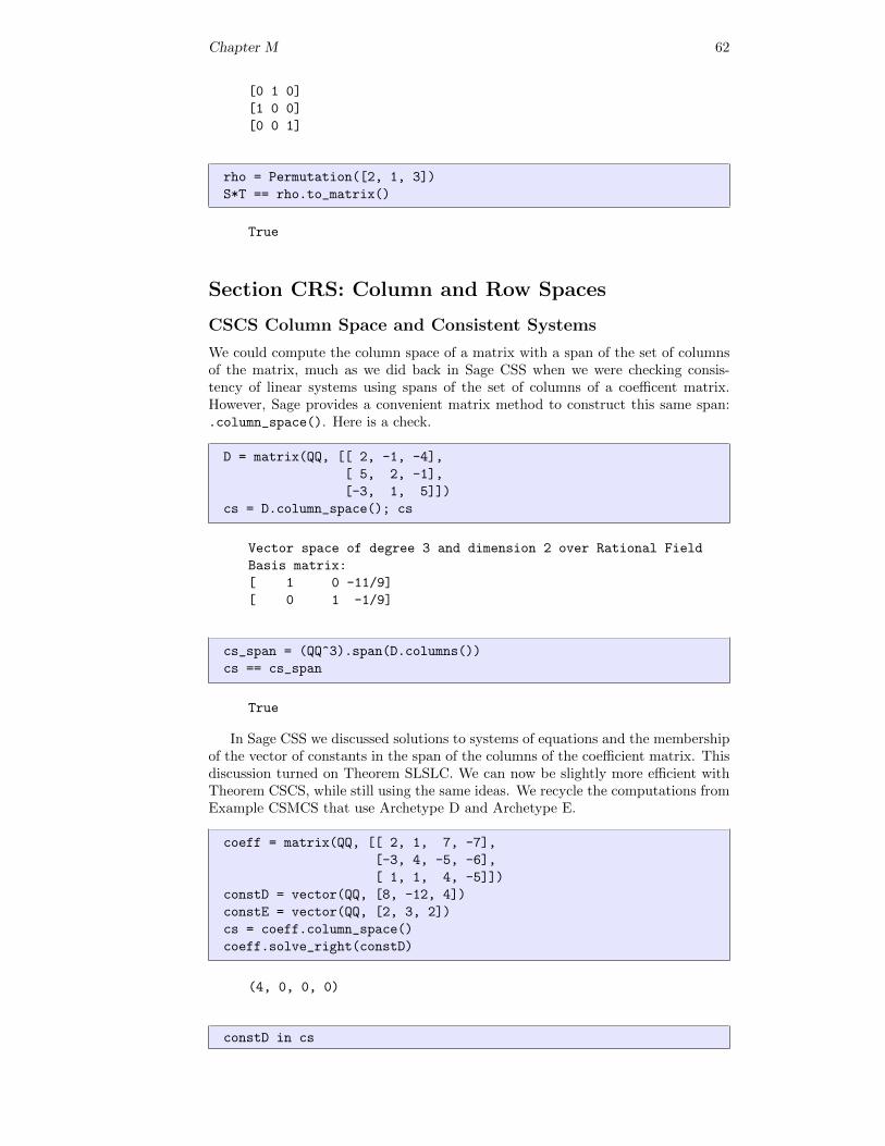
Chapter M 62
[0 1 0]
[1 0 0]
[0 0 1]
rho = Permutation([2, 1, 3])
S*T == rho.to_matrix()
True
Section CRS: Column and Row Spaces
CSCS Column Space and Consistent Systems
We could compute the column space of a matrix with a span of the set of columnsof the matrix, much as we did back in Sage CSS when we were checking consis-tency of linear systems using spans of the set of columns of a coefficent matrix.However, Sage provides a convenient matrix method to construct this same span:.column_space(). Here is a check.
D = matrix(QQ, [[ 2, -1, -4],
[ 5, 2, -1],
[-3, 1, 5]])
cs = D.column_space(); cs
Vector space of degree 3 and dimension 2 over Rational Field
Basis matrix:
[ 1 0 -11/9]
[ 0 1 -1/9]
cs_span = (QQ^3).span(D.columns())
cs == cs_span
True
In Sage CSS we discussed solutions to systems of equations and the membershipof the vector of constants in the span of the columns of the coefficient matrix. Thisdiscussion turned on Theorem SLSLC. We can now be slightly more efficient withTheorem CSCS, while still using the same ideas. We recycle the computations fromExample CSMCS that use Archetype D and Archetype E.
coeff = matrix(QQ, [[ 2, 1, 7, -7],
[-3, 4, -5, -6],
[ 1, 1, 4, -5]])
constD = vector(QQ, [8, -12, 4])
constE = vector(QQ, [2, 3, 2])
cs = coeff.column_space()
coeff.solve_right(constD)
(4, 0, 0, 0)
constD in cs
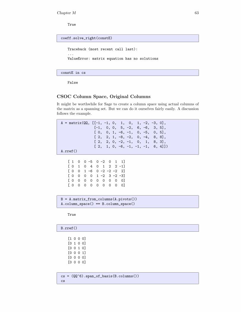
Chapter M 63
True
coeff.solve_right(constE)
Traceback (most recent call last):
...
ValueError: matrix equation has no solutions
constE in cs
False
CSOC Column Space, Original Columns
It might be worthwhile for Sage to create a column space using actual columns ofthe matrix as a spanning set. But we can do it ourselves fairly easily. A discussionfollows the example.
A = matrix(QQ, [[-1, -1, 0, 1, 0, 1, -2, -3, 0],
[-1, 0, 0, 5, -2, 6, -6, 3, 5],
[ 0, 0, 1, -6, -1, 0, -5, 0, 5],
[ 2, 2, 1, -8, -2, 0, -4, 8, 8],
[ 2, 2, 0, -2, -1, 0, 1, 8, 3],
[ 2, 1, 0, -6, -1, -1, -1, 6, 4]])
A.rref()
[ 1 0 0 -5 0 -2 0 1 1]
[ 0 1 0 4 0 1 2 2 -1]
[ 0 0 1 -6 0 -2 -2 -2 2]
[ 0 0 0 0 1 -2 3 -2 -3]
[ 0 0 0 0 0 0 0 0 0]
[ 0 0 0 0 0 0 0 0 0]
B = A.matrix_from_columns(A.pivots())
A.column_space() == B.column_space()
True
B.rref()
[1 0 0 0]
[0 1 0 0]
[0 0 1 0]
[0 0 0 1]
[0 0 0 0]
[0 0 0 0]
cs = (QQ^6).span_of_basis(B.columns())
cs
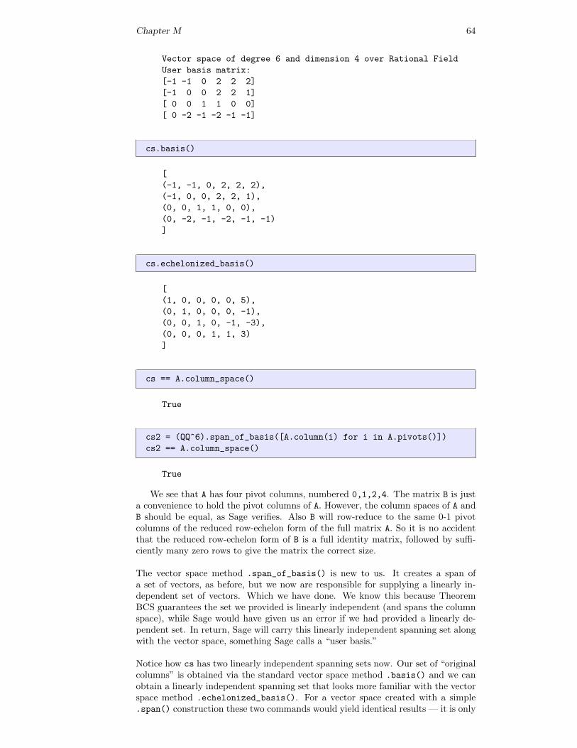
Chapter M 64
Vector space of degree 6 and dimension 4 over Rational Field
User basis matrix:
[-1 -1 0 2 2 2]
[-1 0 0 2 2 1]
[ 0 0 1 1 0 0]
[ 0 -2 -1 -2 -1 -1]
cs.basis()
[
(-1, -1, 0, 2, 2, 2),
(-1, 0, 0, 2, 2, 1),
(0, 0, 1, 1, 0, 0),
(0, -2, -1, -2, -1, -1)
]
cs.echelonized_basis()
[
(1, 0, 0, 0, 0, 5),
(0, 1, 0, 0, 0, -1),
(0, 0, 1, 0, -1, -3),
(0, 0, 0, 1, 1, 3)
]
cs == A.column_space()
True
cs2 = (QQ^6).span_of_basis([A.column(i) for i in A.pivots()])
cs2 == A.column_space()
True
We see that A has four pivot columns, numbered 0,1,2,4. The matrix B is justa convenience to hold the pivot columns of A. However, the column spaces of A andB should be equal, as Sage verifies. Also B will row-reduce to the same 0-1 pivotcolumns of the reduced row-echelon form of the full matrix A. So it is no accidentthat the reduced row-echelon form of B is a full identity matrix, followed by suffi-ciently many zero rows to give the matrix the correct size.
The vector space method .span_of_basis() is new to us. It creates a span ofa set of vectors, as before, but we now are responsible for supplying a linearly in-dependent set of vectors. Which we have done. We know this because TheoremBCS guarantees the set we provided is linearly independent (and spans the columnspace), while Sage would have given us an error if we had provided a linearly de-pendent set. In return, Sage will carry this linearly independent spanning set alongwith the vector space, something Sage calls a “user basis.”
Notice how cs has two linearly independent spanning sets now. Our set of “originalcolumns” is obtained via the standard vector space method .basis() and we canobtain a linearly independent spanning set that looks more familiar with the vectorspace method .echelonized_basis(). For a vector space created with a simple.span() construction these two commands would yield identical results — it is only
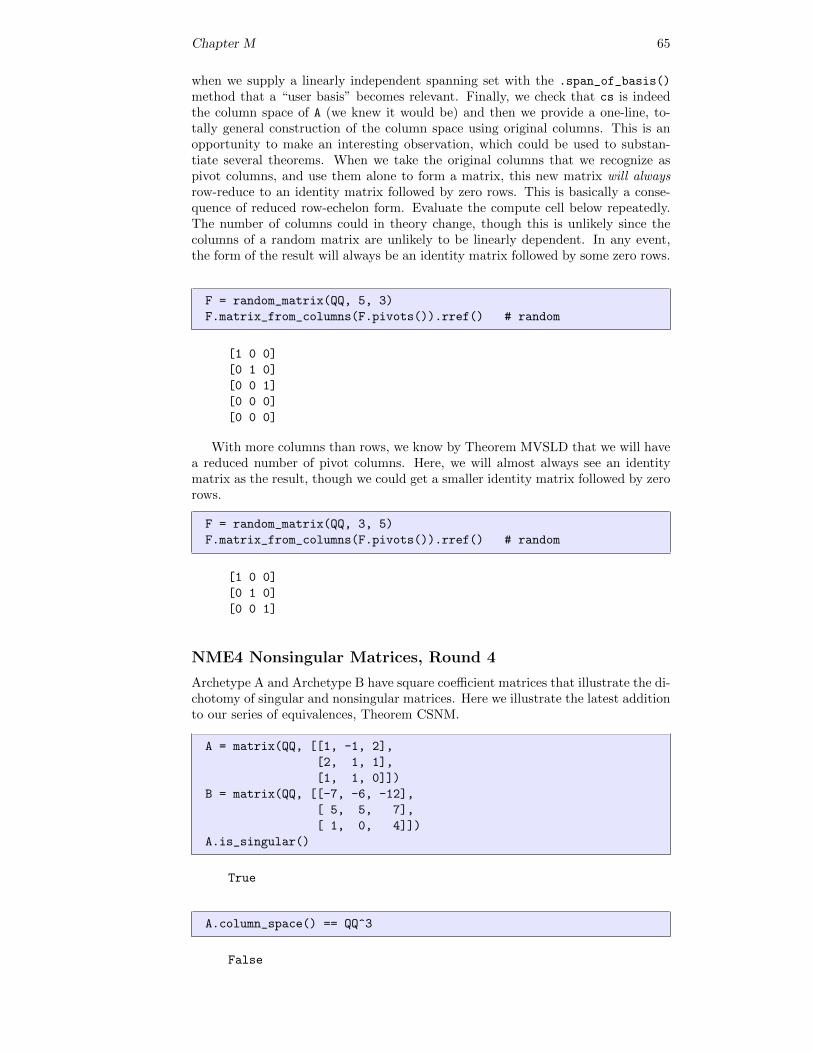
Chapter M 65
when we supply a linearly independent spanning set with the .span_of_basis()
method that a “user basis” becomes relevant. Finally, we check that cs is indeedthe column space of A (we knew it would be) and then we provide a one-line, to-tally general construction of the column space using original columns. This is anopportunity to make an interesting observation, which could be used to substan-tiate several theorems. When we take the original columns that we recognize aspivot columns, and use them alone to form a matrix, this new matrix will alwaysrow-reduce to an identity matrix followed by zero rows. This is basically a conse-quence of reduced row-echelon form. Evaluate the compute cell below repeatedly.The number of columns could in theory change, though this is unlikely since thecolumns of a random matrix are unlikely to be linearly dependent. In any event,the form of the result will always be an identity matrix followed by some zero rows.
F = random_matrix(QQ, 5, 3)
F.matrix_from_columns(F.pivots()).rref() # random
[1 0 0]
[0 1 0]
[0 0 1]
[0 0 0]
[0 0 0]
With more columns than rows, we know by Theorem MVSLD that we will havea reduced number of pivot columns. Here, we will almost always see an identitymatrix as the result, though we could get a smaller identity matrix followed by zerorows.
F = random_matrix(QQ, 3, 5)
F.matrix_from_columns(F.pivots()).rref() # random
[1 0 0]
[0 1 0]
[0 0 1]
NME4 Nonsingular Matrices, Round 4
Archetype A and Archetype B have square coefficient matrices that illustrate the di-chotomy of singular and nonsingular matrices. Here we illustrate the latest additionto our series of equivalences, Theorem CSNM.
A = matrix(QQ, [[1, -1, 2],
[2, 1, 1],
[1, 1, 0]])
B = matrix(QQ, [[-7, -6, -12],
[ 5, 5, 7],
[ 1, 0, 4]])
A.is_singular()
True
A.column_space() == QQ^3
False
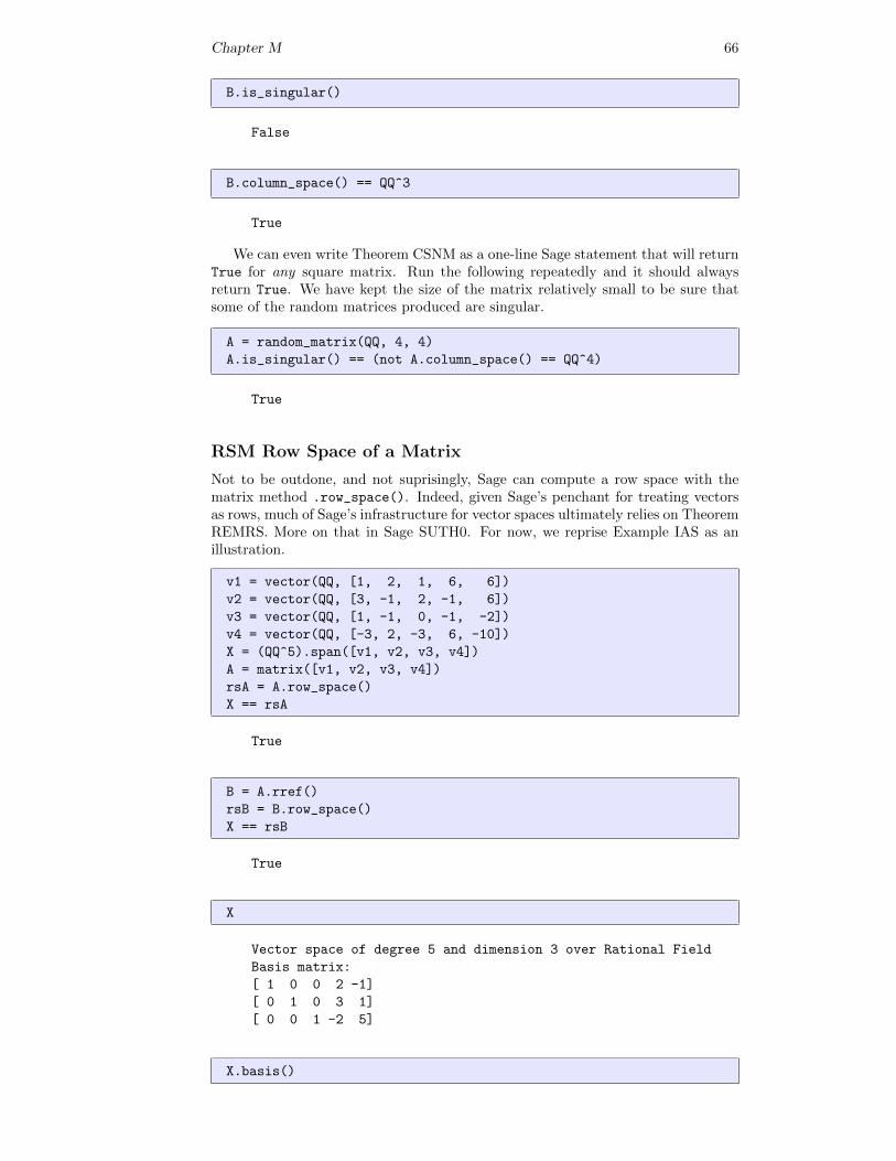
Chapter M 66
B.is_singular()
False
B.column_space() == QQ^3
True
We can even write Theorem CSNM as a one-line Sage statement that will returnTrue for any square matrix. Run the following repeatedly and it should alwaysreturn True. We have kept the size of the matrix relatively small to be sure thatsome of the random matrices produced are singular.
A = random_matrix(QQ, 4, 4)
A.is_singular() == (not A.column_space() == QQ^4)
True
RSM Row Space of a Matrix
Not to be outdone, and not suprisingly, Sage can compute a row space with thematrix method .row_space(). Indeed, given Sage’s penchant for treating vectorsas rows, much of Sage’s infrastructure for vector spaces ultimately relies on TheoremREMRS. More on that in Sage SUTH0. For now, we reprise Example IAS as anillustration.
v1 = vector(QQ, [1, 2, 1, 6, 6])
v2 = vector(QQ, [3, -1, 2, -1, 6])
v3 = vector(QQ, [1, -1, 0, -1, -2])
v4 = vector(QQ, [-3, 2, -3, 6, -10])
X = (QQ^5).span([v1, v2, v3, v4])
A = matrix([v1, v2, v3, v4])
rsA = A.row_space()
X == rsA
True
B = A.rref()
rsB = B.row_space()
X == rsB
True
X
Vector space of degree 5 and dimension 3 over Rational Field
Basis matrix:
[ 1 0 0 2 -1]
[ 0 1 0 3 1]
[ 0 0 1 -2 5]
X.basis()
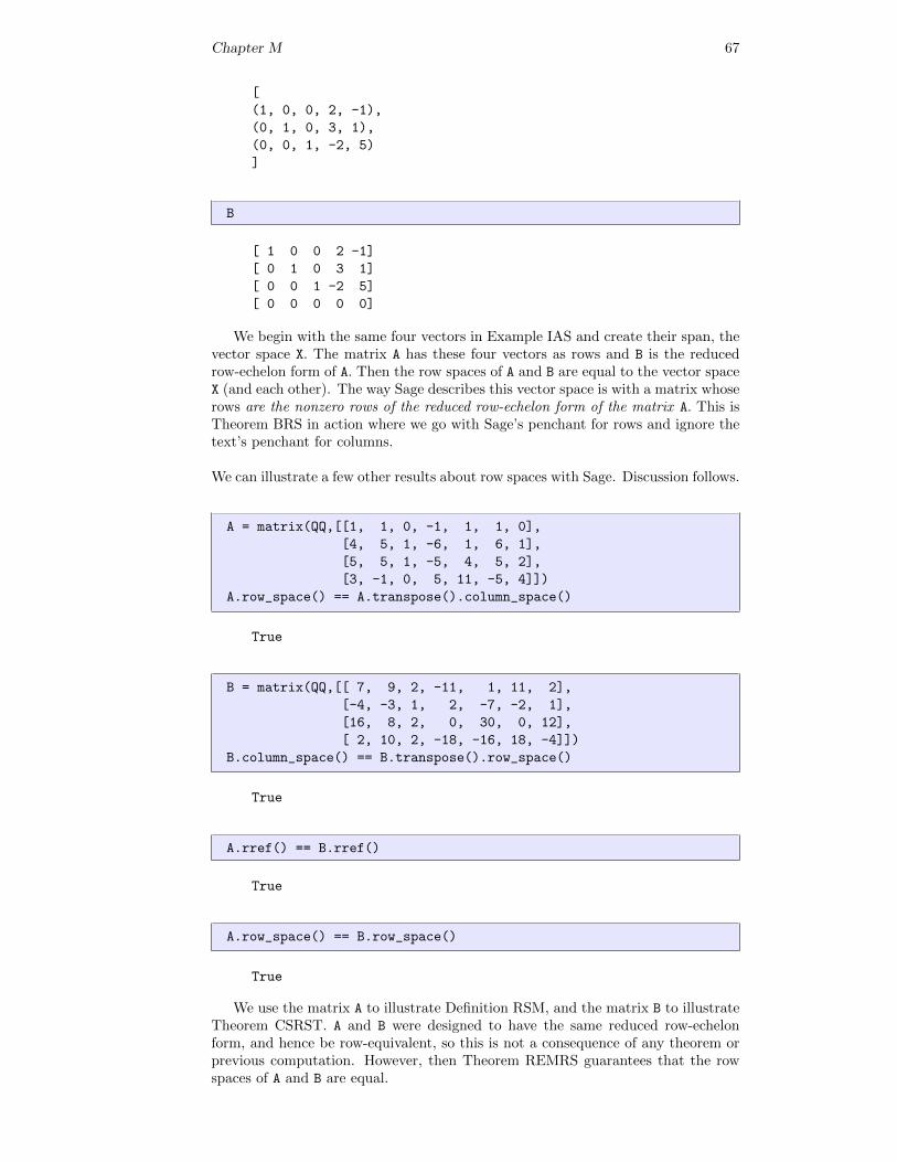
Chapter M 67
[
(1, 0, 0, 2, -1),
(0, 1, 0, 3, 1),
(0, 0, 1, -2, 5)
]
B
[ 1 0 0 2 -1]
[ 0 1 0 3 1]
[ 0 0 1 -2 5]
[ 0 0 0 0 0]
We begin with the same four vectors in Example IAS and create their span, thevector space X. The matrix A has these four vectors as rows and B is the reducedrow-echelon form of A. Then the row spaces of A and B are equal to the vector spaceX (and each other). The way Sage describes this vector space is with a matrix whoserows are the nonzero rows of the reduced row-echelon form of the matrix A. This isTheorem BRS in action where we go with Sage’s penchant for rows and ignore thetext’s penchant for columns.
We can illustrate a few other results about row spaces with Sage. Discussion follows.
A = matrix(QQ,[[1, 1, 0, -1, 1, 1, 0],
[4, 5, 1, -6, 1, 6, 1],
[5, 5, 1, -5, 4, 5, 2],
[3, -1, 0, 5, 11, -5, 4]])
A.row_space() == A.transpose().column_space()
True
B = matrix(QQ,[[ 7, 9, 2, -11, 1, 11, 2],
[-4, -3, 1, 2, -7, -2, 1],
[16, 8, 2, 0, 30, 0, 12],
[ 2, 10, 2, -18, -16, 18, -4]])
B.column_space() == B.transpose().row_space()
True
A.rref() == B.rref()
True
A.row_space() == B.row_space()
True
We use the matrix A to illustrate Definition RSM, and the matrix B to illustrateTheorem CSRST. A and B were designed to have the same reduced row-echelonform, and hence be row-equivalent, so this is not a consequence of any theorem orprevious computation. However, then Theorem REMRS guarantees that the rowspaces of A and B are equal.
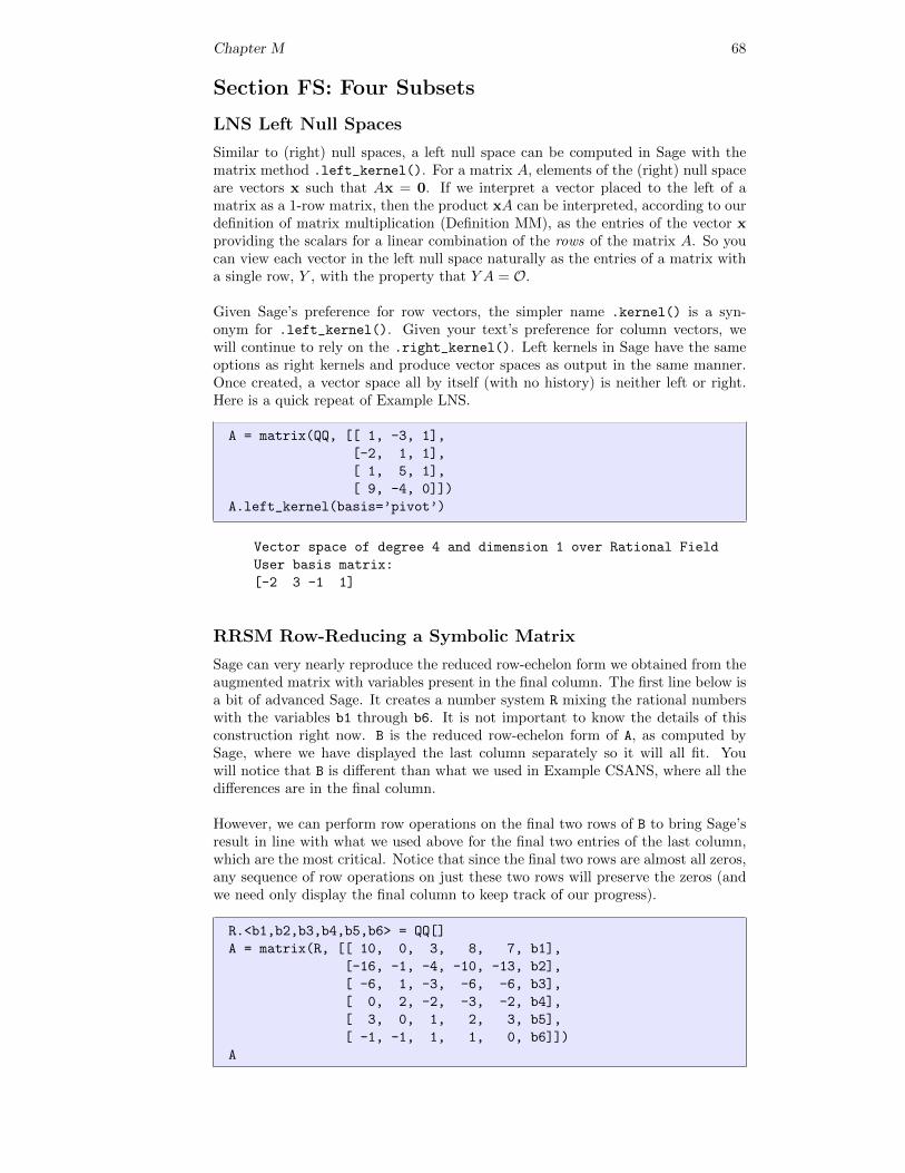
Chapter M 68
Section FS: Four Subsets
LNS Left Null Spaces
Similar to (right) null spaces, a left null space can be computed in Sage with thematrix method .left_kernel(). For a matrix A, elements of the (right) null spaceare vectors x such that Ax = 0. If we interpret a vector placed to the left of amatrix as a 1-row matrix, then the product xA can be interpreted, according to ourdefinition of matrix multiplication (Definition MM), as the entries of the vector xproviding the scalars for a linear combination of the rows of the matrix A. So youcan view each vector in the left null space naturally as the entries of a matrix witha single row, Y , with the property that Y A = O.
Given Sage’s preference for row vectors, the simpler name .kernel() is a syn-onym for .left_kernel(). Given your text’s preference for column vectors, wewill continue to rely on the .right_kernel(). Left kernels in Sage have the sameoptions as right kernels and produce vector spaces as output in the same manner.Once created, a vector space all by itself (with no history) is neither left or right.Here is a quick repeat of Example LNS.
A = matrix(QQ, [[ 1, -3, 1],
[-2, 1, 1],
[ 1, 5, 1],
[ 9, -4, 0]])
A.left_kernel(basis=’pivot’)
Vector space of degree 4 and dimension 1 over Rational Field
User basis matrix:
[-2 3 -1 1]
RRSM Row-Reducing a Symbolic Matrix
Sage can very nearly reproduce the reduced row-echelon form we obtained from theaugmented matrix with variables present in the final column. The first line below isa bit of advanced Sage. It creates a number system R mixing the rational numberswith the variables b1 through b6. It is not important to know the details of thisconstruction right now. B is the reduced row-echelon form of A, as computed bySage, where we have displayed the last column separately so it will all fit. Youwill notice that B is different than what we used in Example CSANS, where all thedifferences are in the final column.
However, we can perform row operations on the final two rows of B to bring Sage’sresult in line with what we used above for the final two entries of the last column,which are the most critical. Notice that since the final two rows are almost all zeros,any sequence of row operations on just these two rows will preserve the zeros (andwe need only display the final column to keep track of our progress).
R.<b1,b2,b3,b4,b5,b6> = QQ[]
A = matrix(R, [[ 10, 0, 3, 8, 7, b1],
[-16, -1, -4, -10, -13, b2],
[ -6, 1, -3, -6, -6, b3],
[ 0, 2, -2, -3, -2, b4],
[ 3, 0, 1, 2, 3, b5],
[ -1, -1, 1, 1, 0, b6]])
A
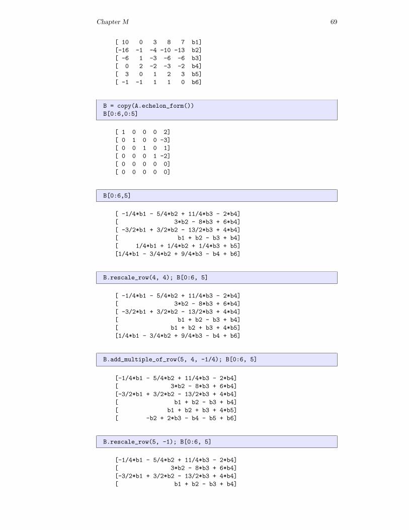
Chapter M 69
[ 10 0 3 8 7 b1]
[-16 -1 -4 -10 -13 b2]
[ -6 1 -3 -6 -6 b3]
[ 0 2 -2 -3 -2 b4]
[ 3 0 1 2 3 b5]
[ -1 -1 1 1 0 b6]
B = copy(A.echelon_form())
B[0:6,0:5]
[ 1 0 0 0 2]
[ 0 1 0 0 -3]
[ 0 0 1 0 1]
[ 0 0 0 1 -2]
[ 0 0 0 0 0]
[ 0 0 0 0 0]
B[0:6,5]
[ -1/4*b1 - 5/4*b2 + 11/4*b3 - 2*b4]
[ 3*b2 - 8*b3 + 6*b4]
[ -3/2*b1 + 3/2*b2 - 13/2*b3 + 4*b4]
[ b1 + b2 - b3 + b4]
[ 1/4*b1 + 1/4*b2 + 1/4*b3 + b5]
[1/4*b1 - 3/4*b2 + 9/4*b3 - b4 + b6]
B.rescale_row(4, 4); B[0:6, 5]
[ -1/4*b1 - 5/4*b2 + 11/4*b3 - 2*b4]
[ 3*b2 - 8*b3 + 6*b4]
[ -3/2*b1 + 3/2*b2 - 13/2*b3 + 4*b4]
[ b1 + b2 - b3 + b4]
[ b1 + b2 + b3 + 4*b5]
[1/4*b1 - 3/4*b2 + 9/4*b3 - b4 + b6]
B.add_multiple_of_row(5, 4, -1/4); B[0:6, 5]
[-1/4*b1 - 5/4*b2 + 11/4*b3 - 2*b4]
[ 3*b2 - 8*b3 + 6*b4]
[-3/2*b1 + 3/2*b2 - 13/2*b3 + 4*b4]
[ b1 + b2 - b3 + b4]
[ b1 + b2 + b3 + 4*b5]
[ -b2 + 2*b3 - b4 - b5 + b6]
B.rescale_row(5, -1); B[0:6, 5]
[-1/4*b1 - 5/4*b2 + 11/4*b3 - 2*b4]
[ 3*b2 - 8*b3 + 6*b4]
[-3/2*b1 + 3/2*b2 - 13/2*b3 + 4*b4]
[ b1 + b2 - b3 + b4]
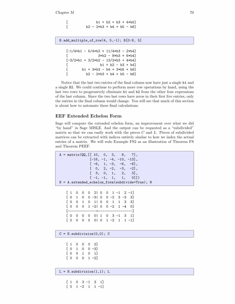
Chapter M 70
[ b1 + b2 + b3 + 4*b5]
[ b2 - 2*b3 + b4 + b5 - b6]
B.add_multiple_of_row(4, 5,-1); B[0:6, 5]
[-1/4*b1 - 5/4*b2 + 11/4*b3 - 2*b4]
[ 3*b2 - 8*b3 + 6*b4]
[-3/2*b1 + 3/2*b2 - 13/2*b3 + 4*b4]
[ b1 + b2 - b3 + b4]
[ b1 + 3*b3 - b4 + 3*b5 + b6]
[ b2 - 2*b3 + b4 + b5 - b6]
Notice that the last two entries of the final column now have just a single b1 anda single B2. We could continue to perform more row operations by hand, using thelast two rows to progressively eliminate b1 and b2 from the other four expressionsof the last column. Since the two last rows have zeros in their first five entries, onlythe entries in the final column would change. You will see that much of this sectionis about how to automate these final calculations.
EEF Extended Echelon Form
Sage will compute the extended echelon form, an improvement over what we did“by hand” in Sage MISLE. And the output can be requested as a “subdivided”matrix so that we can easily work with the pieces C and L. Pieces of subdividedmatrices can be extracted with indices entirely similar to how we index the actualentries of a matrix. We will redo Example FS2 as an illustration of Theorem FSand Theorem PEEF.
A = matrix(QQ,[[ 10, 0, 3, 8, 7],
[-16, -1, -4, -10, -13],
[ -6, 1, -3, -6, -6],
[ 0, 2, -2, -3, -2],
[ 3, 0, 1, 2, 3],
[ -1, -1, 1, 1, 0]])
N = A.extended_echelon_form(subdivide=True); N
[ 1 0 0 0 2| 0 0 1 -1 2 -1]
[ 0 1 0 0 -3| 0 0 -2 3 -3 3]
[ 0 0 1 0 1| 0 0 1 1 3 3]
[ 0 0 0 1 -2| 0 0 -2 1 -4 0]
[--------------+-----------------]
[ 0 0 0 0 0| 1 0 3 -1 3 1]
[ 0 0 0 0 0| 0 1 -2 1 1 -1]
C = N.subdivision(0,0); C
[ 1 0 0 0 2]
[ 0 1 0 0 -3]
[ 0 0 1 0 1]
[ 0 0 0 1 -2]
L = N.subdivision(1,1); L
[ 1 0 3 -1 3 1]
[ 0 1 -2 1 1 -1]
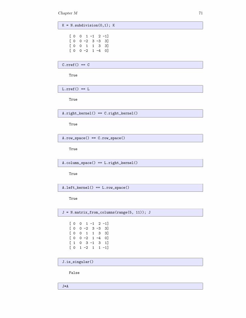
Chapter M 71
K = N.subdivision(0,1); K
[ 0 0 1 -1 2 -1]
[ 0 0 -2 3 -3 3]
[ 0 0 1 1 3 3]
[ 0 0 -2 1 -4 0]
C.rref() == C
True
L.rref() == L
True
A.right_kernel() == C.right_kernel()
True
A.row_space() == C.row_space()
True
A.column_space() == L.right_kernel()
True
A.left_kernel() == L.row_space()
True
J = N.matrix_from_columns(range(5, 11)); J
[ 0 0 1 -1 2 -1]
[ 0 0 -2 3 -3 3]
[ 0 0 1 1 3 3]
[ 0 0 -2 1 -4 0]
[ 1 0 3 -1 3 1]
[ 0 1 -2 1 1 -1]
J.is_singular()
False
J*A
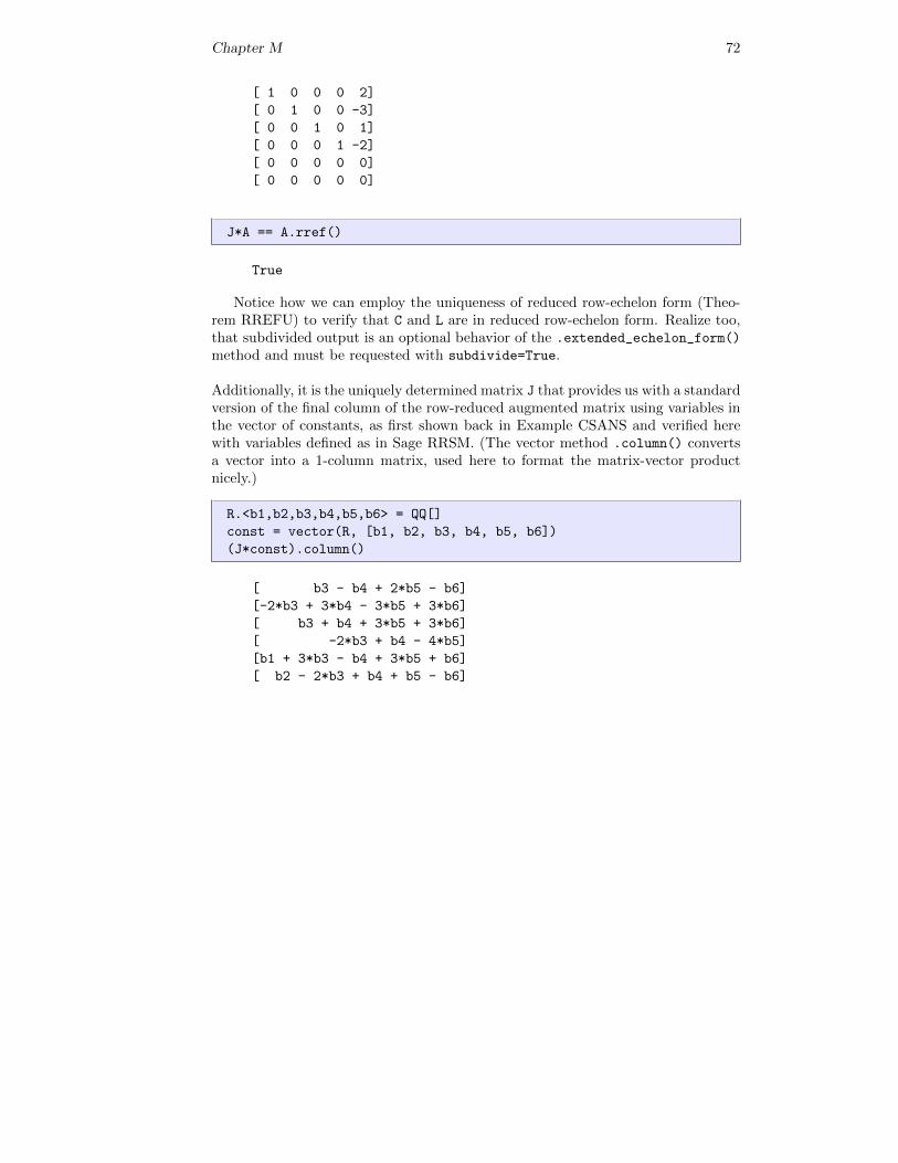
Chapter M 72
[ 1 0 0 0 2]
[ 0 1 0 0 -3]
[ 0 0 1 0 1]
[ 0 0 0 1 -2]
[ 0 0 0 0 0]
[ 0 0 0 0 0]
J*A == A.rref()
True
Notice how we can employ the uniqueness of reduced row-echelon form (Theo-rem RREFU) to verify that C and L are in reduced row-echelon form. Realize too,that subdivided output is an optional behavior of the .extended_echelon_form()
method and must be requested with subdivide=True.
Additionally, it is the uniquely determined matrix J that provides us with a standardversion of the final column of the row-reduced augmented matrix using variables inthe vector of constants, as first shown back in Example CSANS and verified herewith variables defined as in Sage RRSM. (The vector method .column() convertsa vector into a 1-column matrix, used here to format the matrix-vector productnicely.)
R.<b1,b2,b3,b4,b5,b6> = QQ[]
const = vector(R, [b1, b2, b3, b4, b5, b6])
(J*const).column()
[ b3 - b4 + 2*b5 - b6]
[-2*b3 + 3*b4 - 3*b5 + 3*b6]
[ b3 + b4 + 3*b5 + 3*b6]
[ -2*b3 + b4 - 4*b5]
[b1 + 3*b3 - b4 + 3*b5 + b6]
[ b2 - 2*b3 + b4 + b5 - b6]
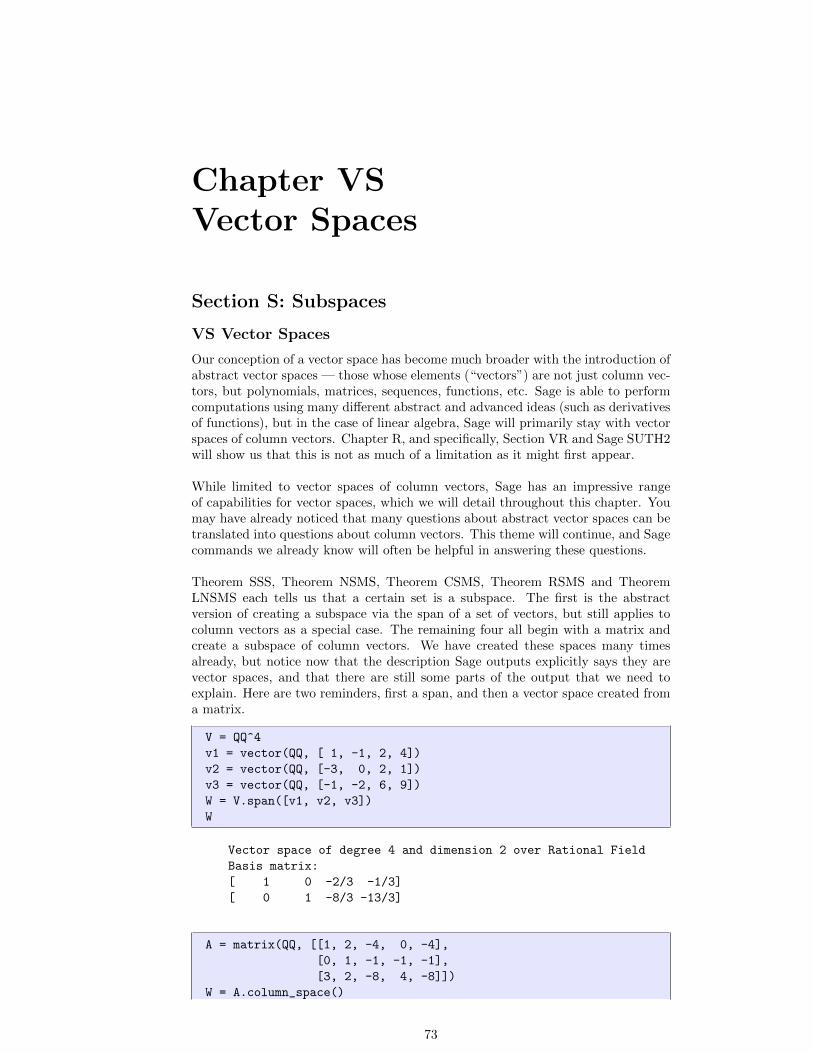
Chapter VSVector Spaces
Section S: Subspaces
VS Vector Spaces
Our conception of a vector space has become much broader with the introduction ofabstract vector spaces — those whose elements (“vectors”) are not just column vec-tors, but polynomials, matrices, sequences, functions, etc. Sage is able to performcomputations using many different abstract and advanced ideas (such as derivativesof functions), but in the case of linear algebra, Sage will primarily stay with vectorspaces of column vectors. Chapter R, and specifically, Section VR and Sage SUTH2will show us that this is not as much of a limitation as it might first appear.
While limited to vector spaces of column vectors, Sage has an impressive rangeof capabilities for vector spaces, which we will detail throughout this chapter. Youmay have already noticed that many questions about abstract vector spaces can betranslated into questions about column vectors. This theme will continue, and Sagecommands we already know will often be helpful in answering these questions.
Theorem SSS, Theorem NSMS, Theorem CSMS, Theorem RSMS and TheoremLNSMS each tells us that a certain set is a subspace. The first is the abstractversion of creating a subspace via the span of a set of vectors, but still applies tocolumn vectors as a special case. The remaining four all begin with a matrix andcreate a subspace of column vectors. We have created these spaces many timesalready, but notice now that the description Sage outputs explicitly says they arevector spaces, and that there are still some parts of the output that we need toexplain. Here are two reminders, first a span, and then a vector space created froma matrix.
V = QQ^4
v1 = vector(QQ, [ 1, -1, 2, 4])
v2 = vector(QQ, [-3, 0, 2, 1])
v3 = vector(QQ, [-1, -2, 6, 9])
W = V.span([v1, v2, v3])
W
Vector space of degree 4 and dimension 2 over Rational Field
Basis matrix:
[ 1 0 -2/3 -1/3]
[ 0 1 -8/3 -13/3]
A = matrix(QQ, [[1, 2, -4, 0, -4],
[0, 1, -1, -1, -1],
[3, 2, -8, 4, -8]])
W = A.column_space()
73
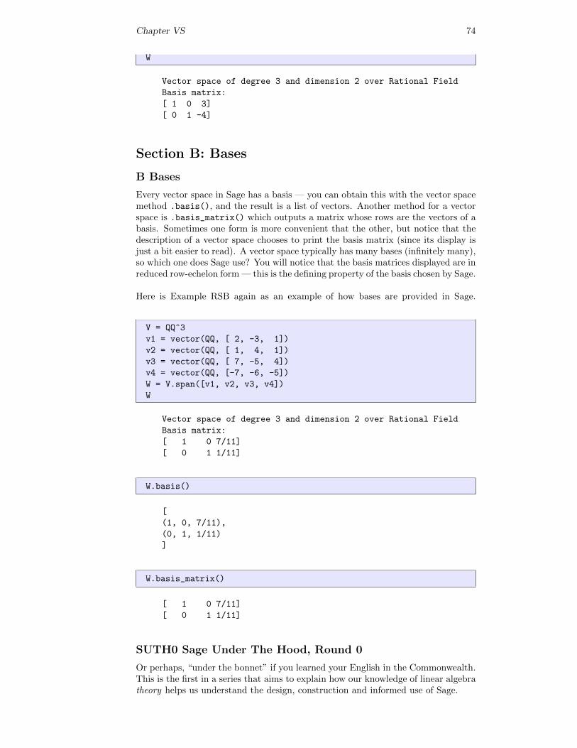
Chapter VS 74
W
Vector space of degree 3 and dimension 2 over Rational Field
Basis matrix:
[ 1 0 3]
[ 0 1 -4]
Section B: Bases
B Bases
Every vector space in Sage has a basis — you can obtain this with the vector spacemethod .basis(), and the result is a list of vectors. Another method for a vectorspace is .basis_matrix() which outputs a matrix whose rows are the vectors of abasis. Sometimes one form is more convenient that the other, but notice that thedescription of a vector space chooses to print the basis matrix (since its display isjust a bit easier to read). A vector space typically has many bases (infinitely many),so which one does Sage use? You will notice that the basis matrices displayed are inreduced row-echelon form — this is the defining property of the basis chosen by Sage.
Here is Example RSB again as an example of how bases are provided in Sage.
V = QQ^3
v1 = vector(QQ, [ 2, -3, 1])
v2 = vector(QQ, [ 1, 4, 1])
v3 = vector(QQ, [ 7, -5, 4])
v4 = vector(QQ, [-7, -6, -5])
W = V.span([v1, v2, v3, v4])
W
Vector space of degree 3 and dimension 2 over Rational Field
Basis matrix:
[ 1 0 7/11]
[ 0 1 1/11]
W.basis()
[
(1, 0, 7/11),
(0, 1, 1/11)
]
W.basis_matrix()
[ 1 0 7/11]
[ 0 1 1/11]
SUTH0 Sage Under The Hood, Round 0
Or perhaps, “under the bonnet” if you learned your English in the Commonwealth.This is the first in a series that aims to explain how our knowledge of linear algebratheory helps us understand the design, construction and informed use of Sage.
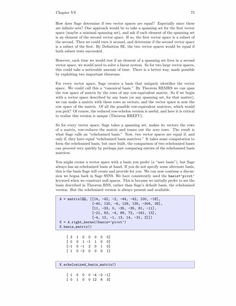
Chapter VS 75
How does Sage determine if two vector spaces are equal? Especially since theseare infinite sets? One approach would be to take a spanning set for the first vectorspace (maybe a minimal spanning set), and ask if each element of the spanning setis an element of the second vector space. If so, the first vector space is a subset ofthe second. Then we could turn it around, and determine if the second vector spaceis a subset of the first. By Definition SE, the two vector spaces would be equal ifboth subset tests succeeded.
However, each time we would test if an element of a spanning set lives in a secondvector space, we would need to solve a linear system. So for two large vector spaces,this could take a noticeable amount of time. There is a better way, made possibleby exploiting two important theorems.
For every vector space, Sage creates a basis that uniquely identifies the vectorspace. We could call this a “canonical basis.” By Theorem REMRS we can spanthe row space of matrix by the rows of any row-equivalent matrix. So if we beginwith a vector space described by any basis (or any spanning set, for that matter),we can make a matrix with these rows as vectors, and the vector space is now therow space of the matrix. Of all the possible row-equivalent matrices, which wouldyou pick? Of course, the reduced row-echelon version is useful, and here it is criticalto realize this version is unique (Theorem RREFU).
So for every vector space, Sage takes a spanning set, makes its vectors the rowsof a matrix, row-reduces the matrix and tosses out the zero rows. The result iswhat Sage calls an “echelonized basis.” Now, two vector spaces are equal if, andonly if, they have equal “echelonized basis matrices.” It takes some computation toform the echelonized basis, but once built, the comparison of two echelonized basescan proceed very quickly by perhaps just comparing entries of the echelonized basismatrices.
You might create a vector space with a basis you prefer (a “user basis”), but Sagealways has an echelonized basis at hand. If you do not specify some alternate basis,this is the basis Sage will create and provide for you. We can now continue a discus-sion we began back in Sage SSNS. We have consistently used the basis=’pivot’
keyword when we construct null spaces. This is because we initially prefer to see thebasis described in Theorem BNS, rather than Sage’s default basis, the echelonizedversion. But the echelonized version is always present and available.
A = matrix(QQ, [[14, -42, -2, -44, -42, 100, -18],
[-40, 120, -6, 129, 135, -304, 28],
[11, -33, 0, -35, -35, 81, -11],
[-21, 63, -4, 68, 72, -161, 13],
[-4, 12, -1, 13, 14, -31, 2]])
K = A.right_kernel(basis=’pivot’)
K.basis_matrix()
[ 3 1 0 0 0 0 0]
[ 0 0 1 -1 1 0 0]
[-1 0 -1 2 0 1 0]
[ 1 0 -2 0 0 0 1]
K.echelonized_basis_matrix()
[ 1 0 0 0 -4 -2 -1]
[ 0 1 0 0 12 6 3]
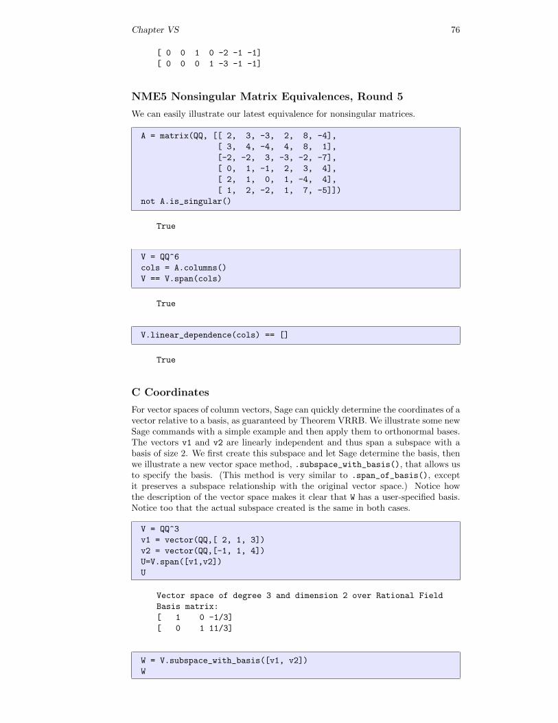
Chapter VS 76
[ 0 0 1 0 -2 -1 -1]
[ 0 0 0 1 -3 -1 -1]
NME5 Nonsingular Matrix Equivalences, Round 5
We can easily illustrate our latest equivalence for nonsingular matrices.
A = matrix(QQ, [[ 2, 3, -3, 2, 8, -4],
[ 3, 4, -4, 4, 8, 1],
[-2, -2, 3, -3, -2, -7],
[ 0, 1, -1, 2, 3, 4],
[ 2, 1, 0, 1, -4, 4],
[ 1, 2, -2, 1, 7, -5]])
not A.is_singular()
True
V = QQ^6
cols = A.columns()
V == V.span(cols)
True
V.linear_dependence(cols) == []
True
C Coordinates
For vector spaces of column vectors, Sage can quickly determine the coordinates of avector relative to a basis, as guaranteed by Theorem VRRB. We illustrate some newSage commands with a simple example and then apply them to orthonormal bases.The vectors v1 and v2 are linearly independent and thus span a subspace with abasis of size 2. We first create this subspace and let Sage determine the basis, thenwe illustrate a new vector space method, .subspace_with_basis(), that allows usto specify the basis. (This method is very similar to .span_of_basis(), exceptit preserves a subspace relationship with the original vector space.) Notice howthe description of the vector space makes it clear that W has a user-specified basis.Notice too that the actual subspace created is the same in both cases.
V = QQ^3
v1 = vector(QQ,[ 2, 1, 3])
v2 = vector(QQ,[-1, 1, 4])
U=V.span([v1,v2])
U
Vector space of degree 3 and dimension 2 over Rational Field
Basis matrix:
[ 1 0 -1/3]
[ 0 1 11/3]
W = V.subspace_with_basis([v1, v2])
W
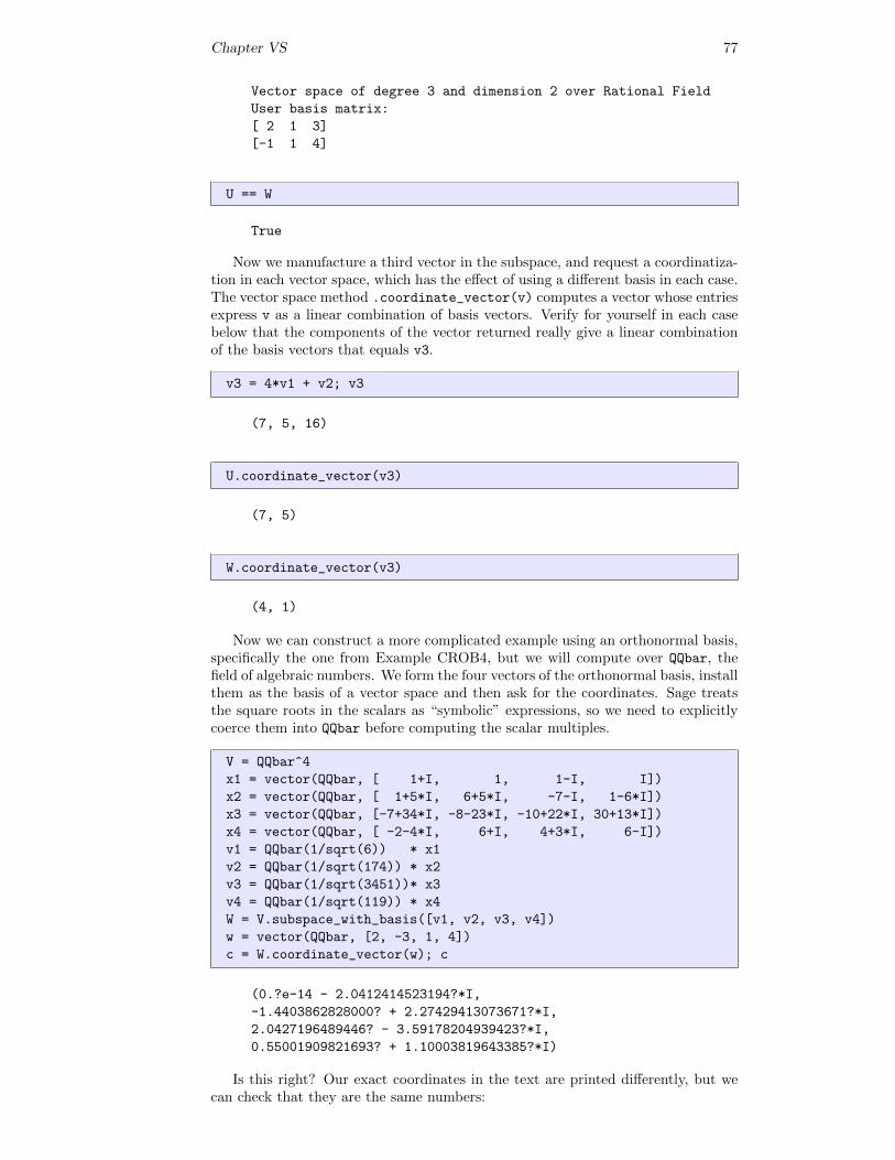
Chapter VS 77
Vector space of degree 3 and dimension 2 over Rational Field
User basis matrix:
[ 2 1 3]
[-1 1 4]
U == W
True
Now we manufacture a third vector in the subspace, and request a coordinatiza-tion in each vector space, which has the effect of using a different basis in each case.The vector space method .coordinate_vector(v) computes a vector whose entriesexpress v as a linear combination of basis vectors. Verify for yourself in each casebelow that the components of the vector returned really give a linear combinationof the basis vectors that equals v3.
v3 = 4*v1 + v2; v3
(7, 5, 16)
U.coordinate_vector(v3)
(7, 5)
W.coordinate_vector(v3)
(4, 1)
Now we can construct a more complicated example using an orthonormal basis,specifically the one from Example CROB4, but we will compute over QQbar, thefield of algebraic numbers. We form the four vectors of the orthonormal basis, installthem as the basis of a vector space and then ask for the coordinates. Sage treatsthe square roots in the scalars as “symbolic” expressions, so we need to explicitlycoerce them into QQbar before computing the scalar multiples.
V = QQbar^4
x1 = vector(QQbar, [ 1+I, 1, 1-I, I])
x2 = vector(QQbar, [ 1+5*I, 6+5*I, -7-I, 1-6*I])
x3 = vector(QQbar, [-7+34*I, -8-23*I, -10+22*I, 30+13*I])
x4 = vector(QQbar, [ -2-4*I, 6+I, 4+3*I, 6-I])
v1 = QQbar(1/sqrt(6)) * x1
v2 = QQbar(1/sqrt(174)) * x2
v3 = QQbar(1/sqrt(3451))* x3
v4 = QQbar(1/sqrt(119)) * x4
W = V.subspace_with_basis([v1, v2, v3, v4])
w = vector(QQbar, [2, -3, 1, 4])
c = W.coordinate_vector(w); c
(0.?e-14 - 2.0412414523194?*I,
-1.4403862828000? + 2.27429413073671?*I,
2.0427196489446? - 3.59178204939423?*I,
0.55001909821693? + 1.10003819643385?*I)
Is this right? Our exact coordinates in the text are printed differently, but wecan check that they are the same numbers:
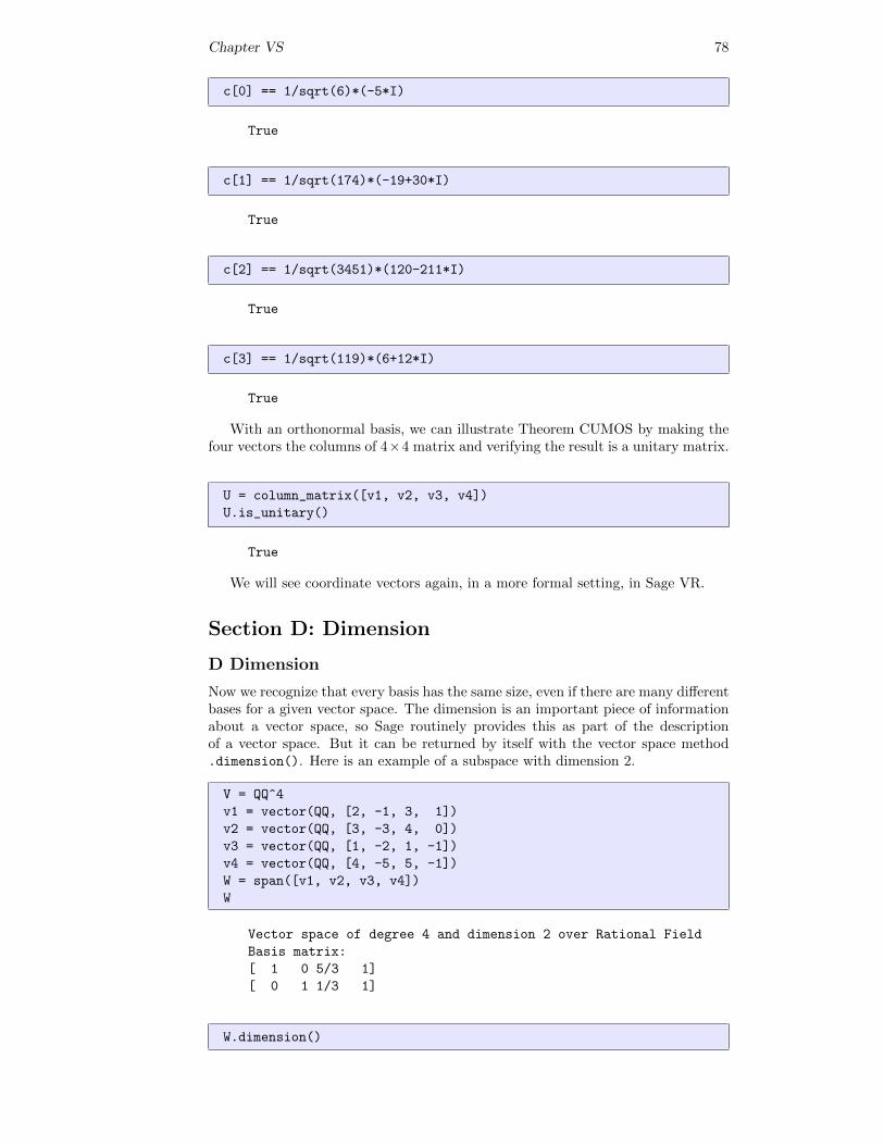
Chapter VS 78
c[0] == 1/sqrt(6)*(-5*I)
True
c[1] == 1/sqrt(174)*(-19+30*I)
True
c[2] == 1/sqrt(3451)*(120-211*I)
True
c[3] == 1/sqrt(119)*(6+12*I)
True
With an orthonormal basis, we can illustrate Theorem CUMOS by making thefour vectors the columns of 4×4 matrix and verifying the result is a unitary matrix.
U = column_matrix([v1, v2, v3, v4])
U.is_unitary()
True
We will see coordinate vectors again, in a more formal setting, in Sage VR.
Section D: Dimension
D Dimension
Now we recognize that every basis has the same size, even if there are many differentbases for a given vector space. The dimension is an important piece of informationabout a vector space, so Sage routinely provides this as part of the descriptionof a vector space. But it can be returned by itself with the vector space method.dimension(). Here is an example of a subspace with dimension 2.
V = QQ^4
v1 = vector(QQ, [2, -1, 3, 1])
v2 = vector(QQ, [3, -3, 4, 0])
v3 = vector(QQ, [1, -2, 1, -1])
v4 = vector(QQ, [4, -5, 5, -1])
W = span([v1, v2, v3, v4])
W
Vector space of degree 4 and dimension 2 over Rational Field
Basis matrix:
[ 1 0 5/3 1]
[ 0 1 1/3 1]
W.dimension()
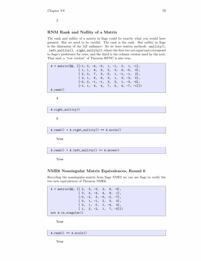
Chapter VS 79
2
RNM Rank and Nullity of a Matrix
The rank and nullity of a matrix in Sage could be exactly what you would haveguessed. But we need to be careful. The rank is the rank. But nullity in Sageis the dimension of the left nullspace. So we have matrix methods .nullity(),.left_nullity(), .right_nullity(), where the first two are equal and correspondto Sage’s preference for rows, and the third is the column version used by the text.That said, a “row version” of Theorem RPNC is also true.
A = matrix(QQ, [[-1, 0, -4, -3, 1, -1, 0, 1, -1],
[ 1, 1, 6, 6, 5, 3, 4, -5, 3],
[ 2, 0, 7, 5, -3, 1, -1, -1, 2],
[ 2, 1, 6, 6, 3, 1, 3, -3, 5],
[-2, 0, -1, -1, 3, 3, 1, -3, -4],
[-1, 1, 4, 4, 7, 5, 4, -7, -1]])
A.rank()
4
A.right_nullity()
5
A.rank() + A.right_nullity() == A.ncols()
True
A.rank() + A.left_nullity() == A.nrows()
True
NME6 Nonsingular Matrix Equivalences, Round 6
Recycling the nonsingular matrix from Sage NME5 we can use Sage to verify thetwo new equivalences of Theorem NME6.
A = matrix(QQ, [[ 2, 3, -3, 2, 8, -4],
[ 3, 4, -4, 4, 8, 1],
[-2, -2, 3, -3, -2, -7],
[ 0, 1, -1, 2, 3, 4],
[ 2, 1, 0, 1, -4, 4],
[ 1, 2, -2, 1, 7, -5]])
not A.is_singular()
True
A.rank() == A.ncols()
True
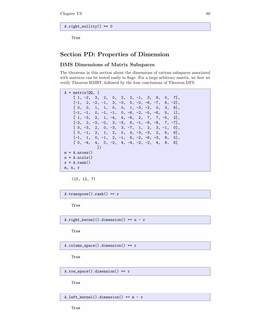
Chapter VS 80
A.right_nullity() == 0
True
Section PD: Properties of Dimension
DMS Dimensions of Matrix Subspaces
The theorems in this section about the dimensions of various subspaces associatedwith matrices can be tested easily in Sage. For a large arbitrary matrix, we first weverify Theorem RMRT, followed by the four conclusions of Theorem DFS.
A = matrix(QQ, [
[ 1, -2, 3, 2, 0, 2, 2, -1, 3, 8, 0, 7],
[-1, 2, -2, -1, 3, -3, 5, -2, -6, -7, 6, -2],
[ 0, 0, 1, 1, 0, 0, 1, -3, -2, 0, 3, 8],
[-1, -1, 0, -1, -1, 0, -6, -2, -5, -6, 5, 1],
[ 1, -3, 2, 1, -4, 4, -6, 2, 7, 7, -5, 2],
[-2, 2, -2, -2, 3, -3, 6, -1, -8, -8, 7, -7],
[ 0, -3, 2, 0, -3, 3, -7, 1, 2, 3, -1, 0],
[ 0, -1, 2, 1, 2, 0, 4, -3, -3, 2, 6, 6],
[-1, 1, 0, -1, 2, -1, 6, -2, -6, -3, 8, 0],
[ 0, -4, 4, 0, -2, 4, -4, -2, -2, 4, 8, 6]
])
m = A.nrows()
n = A.ncols()
r = A.rank()
m, n, r
(10, 12, 7)
A.transpose().rank() == r
True
A.right_kernel().dimension() == n - r
True
A.column_space().dimension() == r
True
A.row_space().dimension() == r
True
A.left_kernel().dimension() == m - r
True
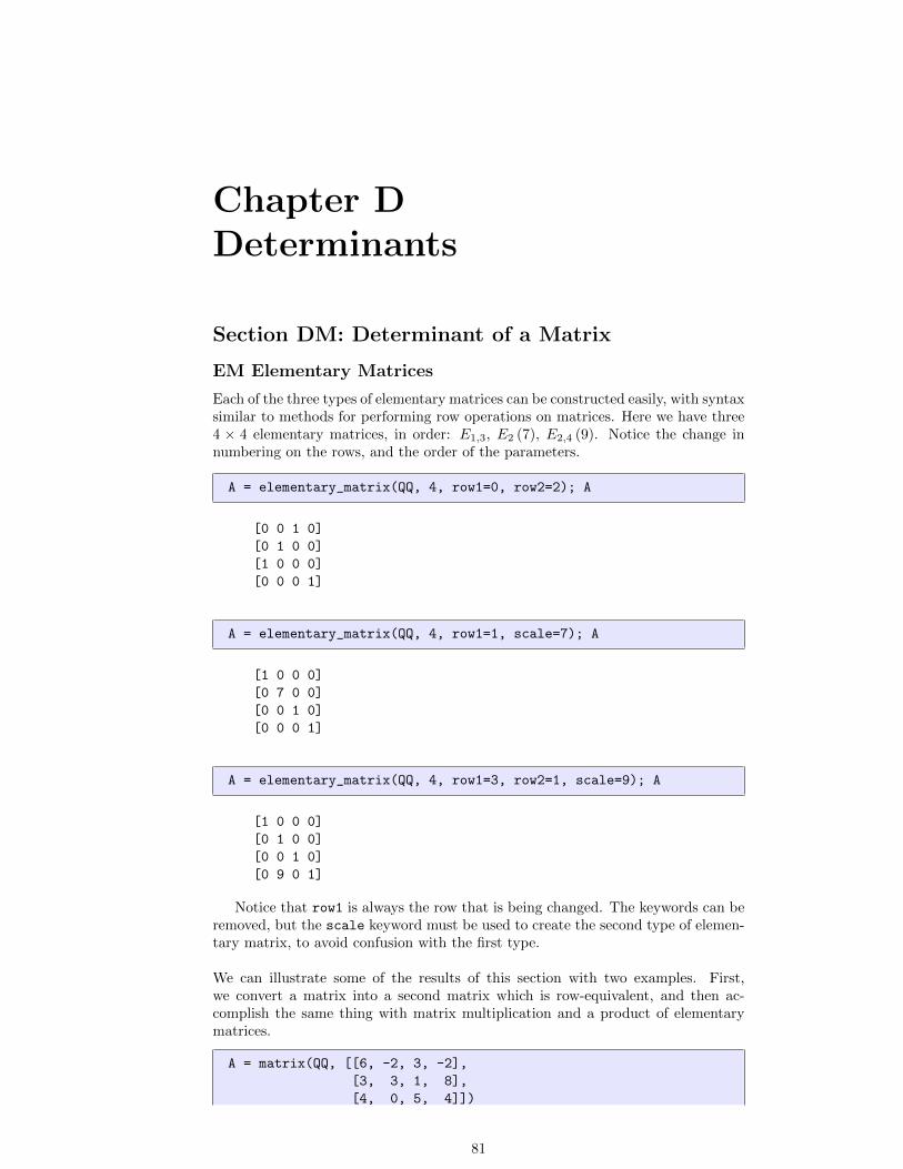
Chapter DDeterminants
Section DM: Determinant of a Matrix
EM Elementary Matrices
Each of the three types of elementary matrices can be constructed easily, with syntaxsimilar to methods for performing row operations on matrices. Here we have three4 × 4 elementary matrices, in order: E1,3, E2 (7), E2,4 (9). Notice the change innumbering on the rows, and the order of the parameters.
A = elementary_matrix(QQ, 4, row1=0, row2=2); A
[0 0 1 0]
[0 1 0 0]
[1 0 0 0]
[0 0 0 1]
A = elementary_matrix(QQ, 4, row1=1, scale=7); A
[1 0 0 0]
[0 7 0 0]
[0 0 1 0]
[0 0 0 1]
A = elementary_matrix(QQ, 4, row1=3, row2=1, scale=9); A
[1 0 0 0]
[0 1 0 0]
[0 0 1 0]
[0 9 0 1]
Notice that row1 is always the row that is being changed. The keywords can beremoved, but the scale keyword must be used to create the second type of elemen-tary matrix, to avoid confusion with the first type.
We can illustrate some of the results of this section with two examples. First,we convert a matrix into a second matrix which is row-equivalent, and then ac-complish the same thing with matrix multiplication and a product of elementarymatrices.
A = matrix(QQ, [[6, -2, 3, -2],
[3, 3, 1, 8],
[4, 0, 5, 4]])
81
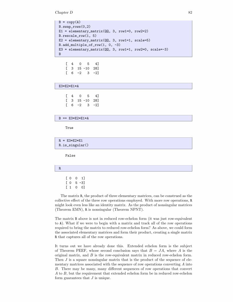
Chapter D 82
B = copy(A)
B.swap_rows(0,2)
E1 = elementary_matrix(QQ, 3, row1=0, row2=2)
B.rescale_row(1, 5)
E2 = elementary_matrix(QQ, 3, row1=1, scale=5)
B.add_multiple_of_row(1, 0, -3)
E3 = elementary_matrix(QQ, 3, row1=1, row2=0, scale=-3)
B
[ 4 0 5 4]
[ 3 15 -10 28]
[ 6 -2 3 -2]
E3*E2*E1*A
[ 4 0 5 4]
[ 3 15 -10 28]
[ 6 -2 3 -2]
B == E3*E2*E1*A
True
R = E3*E2*E1
R.is_singular()
False
R
[ 0 0 1]
[ 0 5 -3]
[ 1 0 0]
The matrix R, the product of three elementary matrices, can be construed as thecollective effect of the three row operations employed. With more row operations, Rmight look even less like an identity matrix. As the product of nonsingular matrices(Theorem EMN), R is nonsingular (Theorem NPNT).
The matrix B above is not in reduced row-echelon form (it was just row-equivalentto A). What if we were to begin with a matrix and track all of the row operationsrequired to bring the matrix to reduced row-echelon form? As above, we could formthe associated elementary matrices and form their product, creating a single matrixR that captures all of the row operations.
It turns out we have already done this. Extended echelon form is the subjectof Theorem PEEF, whose second conclusion says that B = JA, where A is theoriginal matrix, and B is the row-equivalent matrix in reduced row-echelon form.Then J is a square nonsingular matrix that is the product of the sequence of ele-mentary matrices associated with the sequence of row operations converting A intoB. There may be many, many different sequences of row operations that convertA to B, but the requirement that extended echelon form be in reduced row-echelonform guarantees that J is unique.
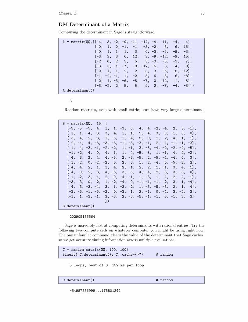
Chapter D 83
DM Determinant of a Matrix
Computing the determinant in Sage is straightforward.
A = matrix(QQ,[[ 4, 3, -2, -9, -11, -14, -4, 11, -4, 4],
[ 0, 1, 0, -1, -1, -3, -2, 3, 6, 15],
[ 0, 1, 1, 1, 3, 0, -3, -5, -9, -3],
[-3, 3, 3, 6, 12, 3, -9, -12, -9, 15],
[-2, 0, 2, 3, 5, 3, -3, -5, -3, 7],
[ 3, 3, -1, -7, -8, -12, -5, 8, -4, 9],
[ 0, -1, 1, 2, 2, 5, 3, -6, -8, -12],
[-1, -2, -1, 1, -2, 5, 6, 3, 6, -8],
[ 2, 1, -3, -6, -8, -7, 0, 12, 11, 8],
[-3, -2, 2, 5, 5, 9, 2, -7, -4, -3]])
A.determinant()
3
Random matrices, even with small entries, can have very large determinants.
B = matrix(QQ, 15, [
[-5, -5, -5, 4, 1, 1, -3, 0, 4, 4, -2, -4, 2, 3, -1],
[ 1, 1, -4, 3, 3, 4, 1, -1, -5, 4, -3, 0, -1, 0, 0],
[ 3, 4, -2, 3, -1, -5, -1, -4, -5, 0, -1, 2, -4, -1, -1],
[ 2, -4, 4, -3, -3, -3, -1, -3, -3, -1, 2, 4, -1, -1, -3],
[ 1, 4, -3, -1, -2, -2, 1, -1, 3, -5, -4, -2, -2, -2, -5],
[-1, -2, 4, 0, 4, 1, 1, 4, -5, 3, 1, -1, 4, 2, -2],
[ 4, 3, 2, 4, 4, -5, 2, -5, -5, 2, -5, -4, -4, 0, 3],
[ 1, -2, 0, -2, -2, 0, 2, 3, 1, 2, -4, 0, -5, -2, 2],
[-4, -4, 2, 1, -1, 4, -2, 1, -2, 2, -1, -1, 3, 4, -1],
[-4, 0, 2, 3, -4, -5, 3, -5, 4, -4, -2, 3, 3, -3, 0],
[ 1, 2, 3, -4, 2, 0, -4, -1, 1, -3, 1, 4, -2, 4, -1],
[-3, 3, 0, 2, 1, -2, -4, 0, -1, -1, -1, 2, 3, 1, -4],
[ 4, 3, -3, -4, 3, 1, -3, 2, 1, -5, -5, -3, 2, 1, 4],
[-3, -5, -1, -5, -2, 0, -3, 1, 2, -1, 0, -4, 3, -2, 3],
[-1, 1, -3, -1, 3, -3, 2, -3, -5, -1, -1, 3, -1, 2, 3]
])
B.determinant()
202905135564
Sage is incredibly fast at computing determinants with rational entries. Try thefollowing two compute cells on whatever computer you might be using right now.The one unfamilar command clears the value of the determinant that Sage caches,so we get accurate timing information across multiple evaluations.
C = random_matrix(QQ, 100, 100)
timeit("C.determinant(); C._cache={}") # random
5 loops, best of 3: 152 ms per loop
C.determinant() # random
-54987836999...175801344
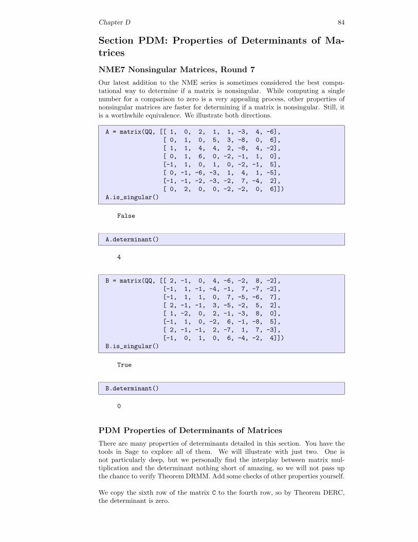
Chapter D 84
Section PDM: Properties of Determinants of Ma-trices
NME7 Nonsingular Matrices, Round 7
Our latest addition to the NME series is sometimes considered the best compu-tational way to determine if a matrix is nonsingular. While computing a singlenumber for a comparison to zero is a very appealing process, other properties ofnonsingular matrices are faster for determining if a matrix is nonsingular. Still, itis a worthwhile equivalence. We illustrate both directions.
A = matrix(QQ, [[ 1, 0, 2, 1, 1, -3, 4, -6],
[ 0, 1, 0, 5, 3, -8, 0, 6],
[ 1, 1, 4, 4, 2, -8, 4, -2],
[ 0, 1, 6, 0, -2, -1, 1, 0],
[-1, 1, 0, 1, 0, -2, -1, 5],
[ 0, -1, -6, -3, 1, 4, 1, -5],
[-1, -1, -2, -3, -2, 7, -4, 2],
[ 0, 2, 0, 0, -2, -2, 0, 6]])
A.is_singular()
False
A.determinant()
4
B = matrix(QQ, [[ 2, -1, 0, 4, -6, -2, 8, -2],
[-1, 1, -1, -4, -1, 7, -7, -2],
[-1, 1, 1, 0, 7, -5, -6, 7],
[ 2, -1, -1, 3, -5, -2, 5, 2],
[ 1, -2, 0, 2, -1, -3, 8, 0],
[-1, 1, 0, -2, 6, -1, -8, 5],
[ 2, -1, -1, 2, -7, 1, 7, -3],
[-1, 0, 1, 0, 6, -4, -2, 4]])
B.is_singular()
True
B.determinant()
0
PDM Properties of Determinants of Matrices
There are many properties of determinants detailed in this section. You have thetools in Sage to explore all of them. We will illustrate with just two. One isnot particularly deep, but we personally find the interplay between matrix mul-tiplication and the determinant nothing short of amazing, so we will not pass upthe chance to verify Theorem DRMM. Add some checks of other properties yourself.
We copy the sixth row of the matrix C to the fourth row, so by Theorem DERC,the determinant is zero.
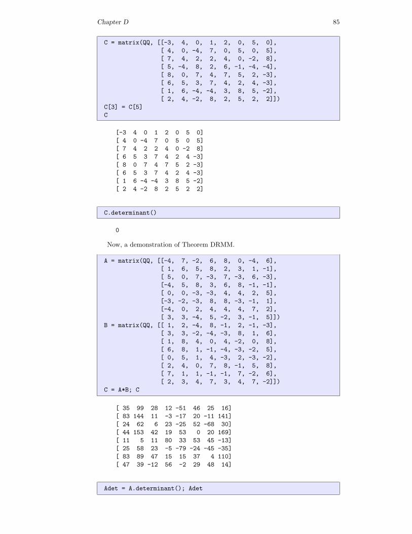
Chapter D 85
C = matrix(QQ, [[-3, 4, 0, 1, 2, 0, 5, 0],
[ 4, 0, -4, 7, 0, 5, 0, 5],
[ 7, 4, 2, 2, 4, 0, -2, 8],
[ 5, -4, 8, 2, 6, -1, -4, -4],
[ 8, 0, 7, 4, 7, 5, 2, -3],
[ 6, 5, 3, 7, 4, 2, 4, -3],
[ 1, 6, -4, -4, 3, 8, 5, -2],
[ 2, 4, -2, 8, 2, 5, 2, 2]])
C[3] = C[5]
C
[-3 4 0 1 2 0 5 0]
[ 4 0 -4 7 0 5 0 5]
[ 7 4 2 2 4 0 -2 8]
[ 6 5 3 7 4 2 4 -3]
[ 8 0 7 4 7 5 2 -3]
[ 6 5 3 7 4 2 4 -3]
[ 1 6 -4 -4 3 8 5 -2]
[ 2 4 -2 8 2 5 2 2]
C.determinant()
0
Now, a demonstration of Theorem DRMM.
A = matrix(QQ, [[-4, 7, -2, 6, 8, 0, -4, 6],
[ 1, 6, 5, 8, 2, 3, 1, -1],
[ 5, 0, 7, -3, 7, -3, 6, -3],
[-4, 5, 8, 3, 6, 8, -1, -1],
[ 0, 0, -3, -3, 4, 4, 2, 5],
[-3, -2, -3, 8, 8, -3, -1, 1],
[-4, 0, 2, 4, 4, 4, 7, 2],
[ 3, 3, -4, 5, -2, 3, -1, 5]])
B = matrix(QQ, [[ 1, 2, -4, 8, -1, 2, -1, -3],
[ 3, 3, -2, -4, -3, 8, 1, 6],
[ 1, 8, 4, 0, 4, -2, 0, 8],
[ 6, 8, 1, -1, -4, -3, -2, 5],
[ 0, 5, 1, 4, -3, 2, -3, -2],
[ 2, 4, 0, 7, 8, -1, 5, 8],
[ 7, 1, 1, -1, -1, 7, -2, 6],
[ 2, 3, 4, 7, 3, 4, 7, -2]])
C = A*B; C
[ 35 99 28 12 -51 46 25 16]
[ 83 144 11 -3 -17 20 -11 141]
[ 24 62 6 23 -25 52 -68 30]
[ 44 153 42 19 53 0 20 169]
[ 11 5 11 80 33 53 45 -13]
[ 25 58 23 -5 -79 -24 -45 -35]
[ 83 89 47 15 15 37 4 110]
[ 47 39 -12 56 -2 29 48 14]
Adet = A.determinant(); Adet
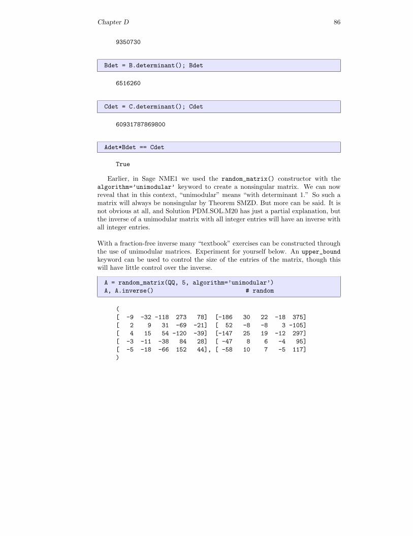
Chapter D 86
9350730
Bdet = B.determinant(); Bdet
6516260
Cdet = C.determinant(); Cdet
60931787869800
Adet*Bdet == Cdet
True
Earlier, in Sage NME1 we used the random_matrix() constructor with thealgorithm=’unimodular’ keyword to create a nonsingular matrix. We can nowreveal that in this context, “unimodular” means “with determinant 1.” So such amatrix will always be nonsingular by Theorem SMZD. But more can be said. It isnot obvious at all, and Solution PDM.SOL.M20 has just a partial explanation, butthe inverse of a unimodular matrix with all integer entries will have an inverse withall integer entries.
With a fraction-free inverse many “textbook” exercises can be constructed throughthe use of unimodular matrices. Experiment for yourself below. An upper_bound
keyword can be used to control the size of the entries of the matrix, though thiswill have little control over the inverse.
A = random_matrix(QQ, 5, algorithm=’unimodular’)
A, A.inverse() # random
(
[ -9 -32 -118 273 78] [-186 30 22 -18 375]
[ 2 9 31 -69 -21] [ 52 -8 -8 3 -105]
[ 4 15 54 -120 -39] [-147 25 19 -12 297]
[ -3 -11 -38 84 28] [ -47 8 6 -4 95]
[ -5 -18 -66 152 44], [ -58 10 7 -5 117]
)
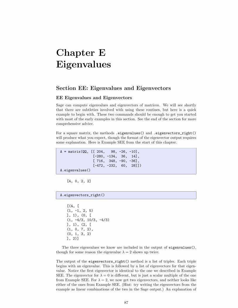
Chapter EEigenvalues
Section EE: Eigenvalues and Eigenvectors
EE Eigenvalues and Eigenvectors
Sage can compute eigenvalues and eigenvectors of matrices. We will see shortlythat there are subtleties involved with using these routines, but here is a quickexample to begin with. These two commands should be enough to get you startedwith most of the early examples in this section. See the end of the section for morecomprehensive advice.
For a square matrix, the methods .eigenvalues() and .eigenvectors_right()
will produce what you expect, though the format of the eigenvector output requiressome explanation. Here is Example SEE from the start of this chapter.
A = matrix(QQ, [[ 204, 98, -26, -10],
[-280, -134, 36, 14],
[ 716, 348, -90, -36],
[-472, -232, 60, 28]])
A.eigenvalues()
[4, 0, 2, 2]
A.eigenvectors_right()
[(4, [
(1, -1, 2, 5)
], 1), (0, [
(1, -4/3, 10/3, -4/3)
], 1), (2, [
(1, 0, 7, 2),
(0, 1, 3, 2)
], 2)]
The three eigenvalues we know are included in the output of eigenvalues(),though for some reason the eigenvalue λ = 2 shows up twice.
The output of the eigenvectors_right() method is a list of triples. Each triplebegins with an eigenvalue. This is followed by a list of eigenvectors for that eigen-value. Notice the first eigenvector is identical to the one we described in ExampleSEE. The eigenvector for λ = 0 is different, but is just a scalar multiple of the onefrom Example SEE. For λ = 2, we now get two eigenvectors, and neither looks likeeither of the ones from Example SEE. (Hint: try writing the eigenvectors from theexample as linear combinations of the two in the Sage output.) An explanation of
87
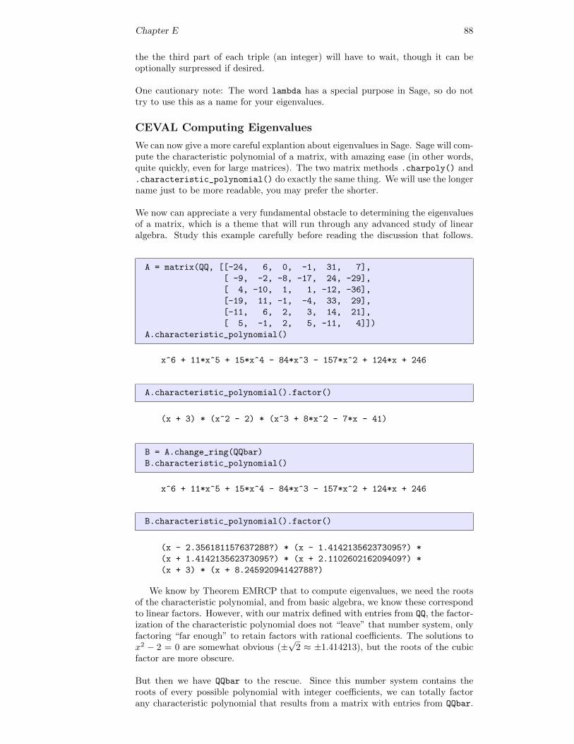
Chapter E 88
the the third part of each triple (an integer) will have to wait, though it can beoptionally surpressed if desired.
One cautionary note: The word lambda has a special purpose in Sage, so do nottry to use this as a name for your eigenvalues.
CEVAL Computing Eigenvalues
We can now give a more careful explantion about eigenvalues in Sage. Sage will com-pute the characteristic polynomial of a matrix, with amazing ease (in other words,quite quickly, even for large matrices). The two matrix methods .charpoly() and.characteristic_polynomial() do exactly the same thing. We will use the longername just to be more readable, you may prefer the shorter.
We now can appreciate a very fundamental obstacle to determining the eigenvaluesof a matrix, which is a theme that will run through any advanced study of linearalgebra. Study this example carefully before reading the discussion that follows.
A = matrix(QQ, [[-24, 6, 0, -1, 31, 7],
[ -9, -2, -8, -17, 24, -29],
[ 4, -10, 1, 1, -12, -36],
[-19, 11, -1, -4, 33, 29],
[-11, 6, 2, 3, 14, 21],
[ 5, -1, 2, 5, -11, 4]])
A.characteristic_polynomial()
x^6 + 11*x^5 + 15*x^4 - 84*x^3 - 157*x^2 + 124*x + 246
A.characteristic_polynomial().factor()
(x + 3) * (x^2 - 2) * (x^3 + 8*x^2 - 7*x - 41)
B = A.change_ring(QQbar)
B.characteristic_polynomial()
x^6 + 11*x^5 + 15*x^4 - 84*x^3 - 157*x^2 + 124*x + 246
B.characteristic_polynomial().factor()
(x - 2.356181157637288?) * (x - 1.414213562373095?) *
(x + 1.414213562373095?) * (x + 2.110260216209409?) *
(x + 3) * (x + 8.24592094142788?)
We know by Theorem EMRCP that to compute eigenvalues, we need the rootsof the characteristic polynomial, and from basic algebra, we know these correspondto linear factors. However, with our matrix defined with entries from QQ, the factor-ization of the characteristic polynomial does not “leave” that number system, onlyfactoring “far enough” to retain factors with rational coefficients. The solutions tox2 − 2 = 0 are somewhat obvious (±
√2 ≈ ±1.414213), but the roots of the cubic
factor are more obscure.
But then we have QQbar to the rescue. Since this number system contains theroots of every possible polynomial with integer coefficients, we can totally factorany characteristic polynomial that results from a matrix with entries from QQbar.
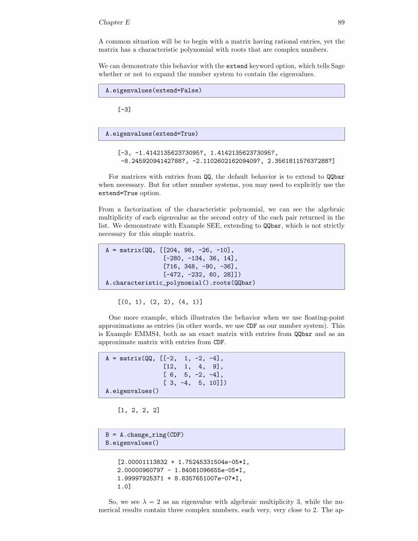
Chapter E 89
A common situation will be to begin with a matrix having rational entries, yet thematrix has a characteristic polynomial with roots that are complex numbers.
We can demonstrate this behavior with the extend keyword option, which tells Sagewhether or not to expand the number system to contain the eigenvalues.
A.eigenvalues(extend=False)
[-3]
A.eigenvalues(extend=True)
[-3, -1.414213562373095?, 1.414213562373095?,
-8.24592094142788?, -2.110260216209409?, 2.356181157637288?]
For matrices with entries from QQ, the default behavior is to extend to QQbar
when necessary. But for other number systems, you may need to explicitly use theextend=True option.
From a factorization of the characteristic polynomial, we can see the algebraicmultiplicity of each eigenvalue as the second entry of the each pair returned in thelist. We demonstrate with Example SEE, extending to QQbar, which is not strictlynecessary for this simple matrix.
A = matrix(QQ, [[204, 98, -26, -10],
[-280, -134, 36, 14],
[716, 348, -90, -36],
[-472, -232, 60, 28]])
A.characteristic_polynomial().roots(QQbar)
[(0, 1), (2, 2), (4, 1)]
One more example, which illustrates the behavior when we use floating-pointapproximations as entries (in other words, we use CDF as our number system). Thisis Example EMMS4, both as an exact matrix with entries from QQbar and as anapproximate matrix with entries from CDF.
A = matrix(QQ, [[-2, 1, -2, -4],
[12, 1, 4, 9],
[ 6, 5, -2, -4],
[ 3, -4, 5, 10]])
A.eigenvalues()
[1, 2, 2, 2]
B = A.change_ring(CDF)
B.eigenvalues()
[2.00001113832 + 1.75245331504e-05*I,
2.00000960797 - 1.84081096655e-05*I,
1.99997925371 + 8.8357651007e-07*I,
1.0]
So, we see λ = 2 as an eigenvalue with algebraic multiplicity 3, while the nu-merical results contain three complex numbers, each very, very close to 2. The ap-
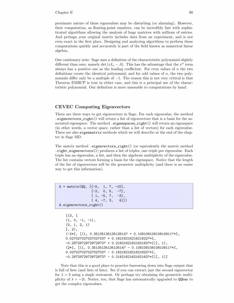
Chapter E 90
proximate nature of these eigenvalues may be disturbing (or alarming). However,their computation, as floating-point numbers, can be incredibly fast with sophis-ticated algorithms allowing the analysis of huge matrices with millions of entries.And perhaps your original matrix includes data from an experiment, and is noteven exact in the first place. Designing and analyzing algorithms to perform thesecomputations quickly and accurately is part of the field known as numerical linearalgebra.
One cautionary note: Sage uses a definition of the characteristic polynomial slightlydifferent than ours, namely det (xIn −A). This has the advantage that the xn termalways has a positive one as the leading coefficient. For even values of n the twodefinitions create the identical polynomial, and for odd values of n, the two poly-nomials differ only be a multiple of −1. The reason this is not very critical is thatTheorem EMRCP is true in either case, and this is a principal use of the charac-teristic polynomial. Our definition is more amenable to computations by hand.
CEVEC Computing Eigenvectors
There are three ways to get eigenvectors in Sage. For each eigenvalue, the method.eigenvectors_right() will return a list of eigenvectors that is a basis for the as-sociated eigenspace. The method .eigenspaces_right() will return an eigenspace(in other words, a vector space, rather than a list of vectors) for each eigenvalue.There are also eigenmatrix methods which we will describe at the end of the chap-ter in Sage MD.
The matrix method .eigenvectors_right() (or equivalently the matrix method.right_eigenvectors()) produces a list of triples, one triple per eigenvalue. Eachtriple has an eigenvalue, a list, and then the algebraic multiplicity of the eigenvalue.The list contains vectors forming a basis for the eigenspace. Notice that the lengthof the list of eigenvectors will be the geometric multiplicity (and there is no easierway to get this information).
A = matrix(QQ, [[-5, 1, 7, -15],
[-2, 0, 5, -7],
[ 1, -5, 7, -3],
[ 4, -7, 3, 4]])
A.eigenvectors_right()
[(3, [
(1, 0, -1, -1),
(0, 1, 2, 1)
], 2),
(-2*I, [(1, 0.3513513513513514? + 0.10810810810810811?*I,
0.02702702702702703? + 0.1621621621621622?*I,
-0.2972972972972973? + 0.2162162162162163?*I)], 1),
(2*I, [(1, 0.3513513513513514? - 0.10810810810810811?*I,
0.02702702702702703? - 0.1621621621621622?*I,
-0.2972972972972973? - 0.2162162162162163?*I)], 1)]
Note that this is a good place to practice burrowing down into Sage output thatis full of lists (and lists of lists). See if you can extract just the second eigenvectorfor λ = 3 using a single statement. Or perhaps try obtaining the geometric multi-plicity of λ = −2i. Notice, too, that Sage has automatically upgraded to QQbar toget the complex eigenvalues.
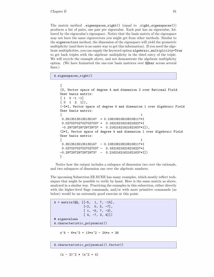
Chapter E 91
The matrix method .eigenspaces_right() (equal to .right_eigenspaces())produces a list of pairs, one pair per eigenvalue. Each pair has an eigenvalue, fol-lowed by the eigenvalue’s eigenspace. Notice that the basis matrix of the eigenspacemay not have the same eigenvectors you might get from other methods. Similar tothe eigenvectors method, the dimension of the eigenspace will yield the geometricmultiplicity (and there is no easier way to get this information). If you need the alge-braic multiplicities, you can supply the keyword option algebraic_multiplicity=True
to get back triples with the algebraic multiplicity in the third entry of the triple.We will recycle the example above, and not demonstrate the algebraic multiplicityoption. (We have formatted the one-row basis matrices over QQbar across severallines.)
A.eigenspaces_right()
[
(3, Vector space of degree 4 and dimension 2 over Rational Field
User basis matrix:
[ 1 0 -1 -1]
[ 0 1 2 1]),
(-2*I, Vector space of degree 4 and dimension 1 over Algebraic Field
User basis matrix:
[ 1
0.3513513513513514? + 0.10810810810810811?*I
0.02702702702702703? + 0.1621621621621622?*I
-0.2972972972972973? + 0.2162162162162163?*I]),
(2*I, Vector space of degree 4 and dimension 1 over Algebraic Field
User basis matrix:
[ 1
0.3513513513513514? - 0.10810810810810811?*I
0.02702702702702703? - 0.1621621621621622?*I
-0.2972972972972973? - 0.2162162162162163?*I])
]
Notice how the output includes a subspace of dimension two over the rationals,and two subspaces of dimension one over the algebraic numbers.
The upcoming Subsection EE.ECEE has many examples, which mostly reflect tech-niques that might be possible to verify by hand. Here is the same matrix as above,analyzed in a similar way. Practicing the examples in this subsection, either directlywith the higher-level Sage commands, and/or with more primitive commands (asbelow) would be an extremely good exercise at this point.
A = matrix(QQ, [[-5, 1, 7, -15],
[-2, 0, 5, -7],
[ 1, -5, 7, -3],
[ 4, -7, 3, 4]])
# eigenvalues
A.characteristic_polynomial()
x^4 - 6*x^3 + 13*x^2 - 24*x + 36
A.characteristic_polynomial().factor()
(x - 3)^2 * (x^2 + 4)
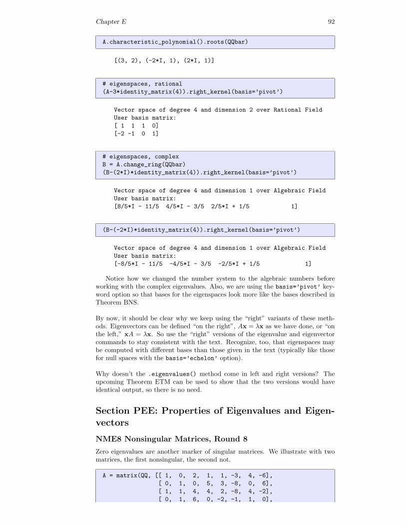
Chapter E 92
A.characteristic_polynomial().roots(QQbar)
[(3, 2), (-2*I, 1), (2*I, 1)]
# eigenspaces, rational
(A-3*identity_matrix(4)).right_kernel(basis=’pivot’)
Vector space of degree 4 and dimension 2 over Rational Field
User basis matrix:
[ 1 1 1 0]
[-2 -1 0 1]
# eigenspaces, complex
B = A.change_ring(QQbar)
(B-(2*I)*identity_matrix(4)).right_kernel(basis=’pivot’)
Vector space of degree 4 and dimension 1 over Algebraic Field
User basis matrix:
[8/5*I - 11/5 4/5*I - 3/5 2/5*I + 1/5 1]
(B-(-2*I)*identity_matrix(4)).right_kernel(basis=’pivot’)
Vector space of degree 4 and dimension 1 over Algebraic Field
User basis matrix:
[-8/5*I - 11/5 -4/5*I - 3/5 -2/5*I + 1/5 1]
Notice how we changed the number system to the algebraic numbers beforeworking with the complex eigenvalues. Also, we are using the basis=’pivot’ key-word option so that bases for the eigenspaces look more like the bases described inTheorem BNS.
By now, it should be clear why we keep using the “right” variants of these meth-ods. Eigenvectors can be defined “on the right”, Ax = λx as we have done, or “onthe left,” xA = λx. So use the “right” versions of the eigenvalue and eigenvectorcommands to stay consistent with the text. Recognize, too, that eigenspaces maybe computed with different bases than those given in the text (typically like thosefor null spaces with the basis=’echelon’ option).
Why doesn’t the .eigenvalues() method come in left and right versions? Theupcoming Theorem ETM can be used to show that the two versions would haveidentical output, so there is no need.
Section PEE: Properties of Eigenvalues and Eigen-vectors
NME8 Nonsingular Matrices, Round 8
Zero eigenvalues are another marker of singular matrices. We illustrate with twomatrices, the first nonsingular, the second not.
A = matrix(QQ, [[ 1, 0, 2, 1, 1, -3, 4, -6],
[ 0, 1, 0, 5, 3, -8, 0, 6],
[ 1, 1, 4, 4, 2, -8, 4, -2],
[ 0, 1, 6, 0, -2, -1, 1, 0],
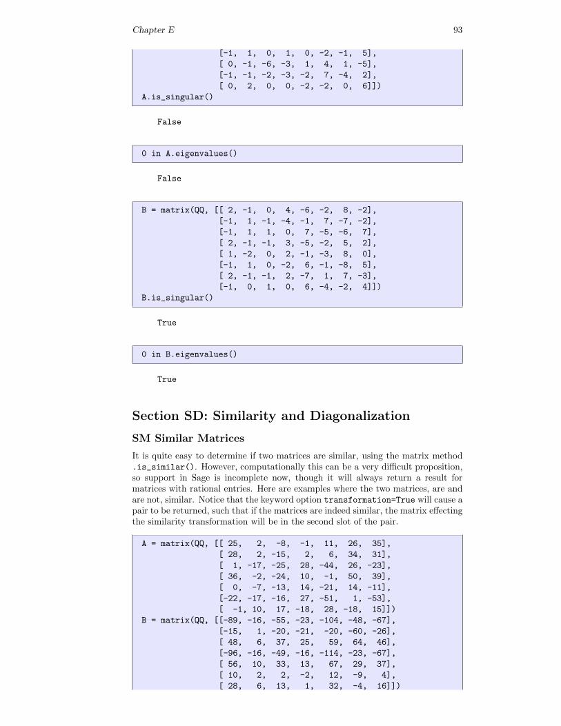
Chapter E 93
[-1, 1, 0, 1, 0, -2, -1, 5],
[ 0, -1, -6, -3, 1, 4, 1, -5],
[-1, -1, -2, -3, -2, 7, -4, 2],
[ 0, 2, 0, 0, -2, -2, 0, 6]])
A.is_singular()
False
0 in A.eigenvalues()
False
B = matrix(QQ, [[ 2, -1, 0, 4, -6, -2, 8, -2],
[-1, 1, -1, -4, -1, 7, -7, -2],
[-1, 1, 1, 0, 7, -5, -6, 7],
[ 2, -1, -1, 3, -5, -2, 5, 2],
[ 1, -2, 0, 2, -1, -3, 8, 0],
[-1, 1, 0, -2, 6, -1, -8, 5],
[ 2, -1, -1, 2, -7, 1, 7, -3],
[-1, 0, 1, 0, 6, -4, -2, 4]])
B.is_singular()
True
0 in B.eigenvalues()
True
Section SD: Similarity and Diagonalization
SM Similar Matrices
It is quite easy to determine if two matrices are similar, using the matrix method.is_similar(). However, computationally this can be a very difficult proposition,so support in Sage is incomplete now, though it will always return a result formatrices with rational entries. Here are examples where the two matrices, are andare not, similar. Notice that the keyword option transformation=True will cause apair to be returned, such that if the matrices are indeed similar, the matrix effectingthe similarity transformation will be in the second slot of the pair.
A = matrix(QQ, [[ 25, 2, -8, -1, 11, 26, 35],
[ 28, 2, -15, 2, 6, 34, 31],
[ 1, -17, -25, 28, -44, 26, -23],
[ 36, -2, -24, 10, -1, 50, 39],
[ 0, -7, -13, 14, -21, 14, -11],
[-22, -17, -16, 27, -51, 1, -53],
[ -1, 10, 17, -18, 28, -18, 15]])
B = matrix(QQ, [[-89, -16, -55, -23, -104, -48, -67],
[-15, 1, -20, -21, -20, -60, -26],
[ 48, 6, 37, 25, 59, 64, 46],
[-96, -16, -49, -16, -114, -23, -67],
[ 56, 10, 33, 13, 67, 29, 37],
[ 10, 2, 2, -2, 12, -9, 4],
[ 28, 6, 13, 1, 32, -4, 16]])
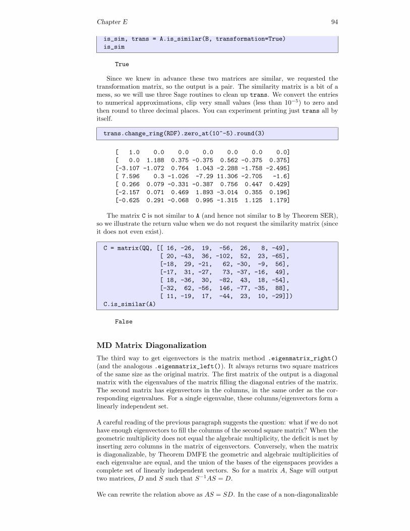
Chapter E 94
is_sim, trans = A.is_similar(B, transformation=True)
is_sim
True
Since we knew in advance these two matrices are similar, we requested thetransformation matrix, so the output is a pair. The similarity matrix is a bit of amess, so we will use three Sage routines to clean up trans. We convert the entriesto numerical approximations, clip very small values (less than 10−5) to zero andthen round to three decimal places. You can experiment printing just trans all byitself.
trans.change_ring(RDF).zero_at(10^-5).round(3)
[ 1.0 0.0 0.0 0.0 0.0 0.0 0.0]
[ 0.0 1.188 0.375 -0.375 0.562 -0.375 0.375]
[-3.107 -1.072 0.764 1.043 -2.288 -1.758 -2.495]
[ 7.596 0.3 -1.026 -7.29 11.306 -2.705 -1.6]
[ 0.266 0.079 -0.331 -0.387 0.756 0.447 0.429]
[-2.157 0.071 0.469 1.893 -3.014 0.355 0.196]
[-0.625 0.291 -0.068 0.995 -1.315 1.125 1.179]
The matrix C is not similar to A (and hence not similar to B by Theorem SER),so we illustrate the return value when we do not request the similarity matrix (sinceit does not even exist).
C = matrix(QQ, [[ 16, -26, 19, -56, 26, 8, -49],
[ 20, -43, 36, -102, 52, 23, -65],
[-18, 29, -21, 62, -30, -9, 56],
[-17, 31, -27, 73, -37, -16, 49],
[ 18, -36, 30, -82, 43, 18, -54],
[-32, 62, -56, 146, -77, -35, 88],
[ 11, -19, 17, -44, 23, 10, -29]])
C.is_similar(A)
False
MD Matrix Diagonalization
The third way to get eigenvectors is the matrix method .eigenmatrix_right()
(and the analogous .eigenmatrix_left()). It always returns two square matricesof the same size as the original matrix. The first matrix of the output is a diagonalmatrix with the eigenvalues of the matrix filling the diagonal entries of the matrix.The second matrix has eigenvectors in the columns, in the same order as the cor-responding eigenvalues. For a single eigenvalue, these columns/eigenvectors form alinearly independent set.
A careful reading of the previous paragraph suggests the question: what if we do nothave enough eigenvectors to fill the columns of the second square matrix? When thegeometric multiplicity does not equal the algebraic multiplicity, the deficit is met byinserting zero columns in the matrix of eigenvectors. Conversely, when the matrixis diagonalizable, by Theorem DMFE the geometric and algebraic multiplicities ofeach eigenvalue are equal, and the union of the bases of the eigenspaces provides acomplete set of linearly independent vectors. So for a matrix A, Sage will outputtwo matrices, D and S such that S−1AS = D.
We can rewrite the relation above as AS = SD. In the case of a non-diagonalizable
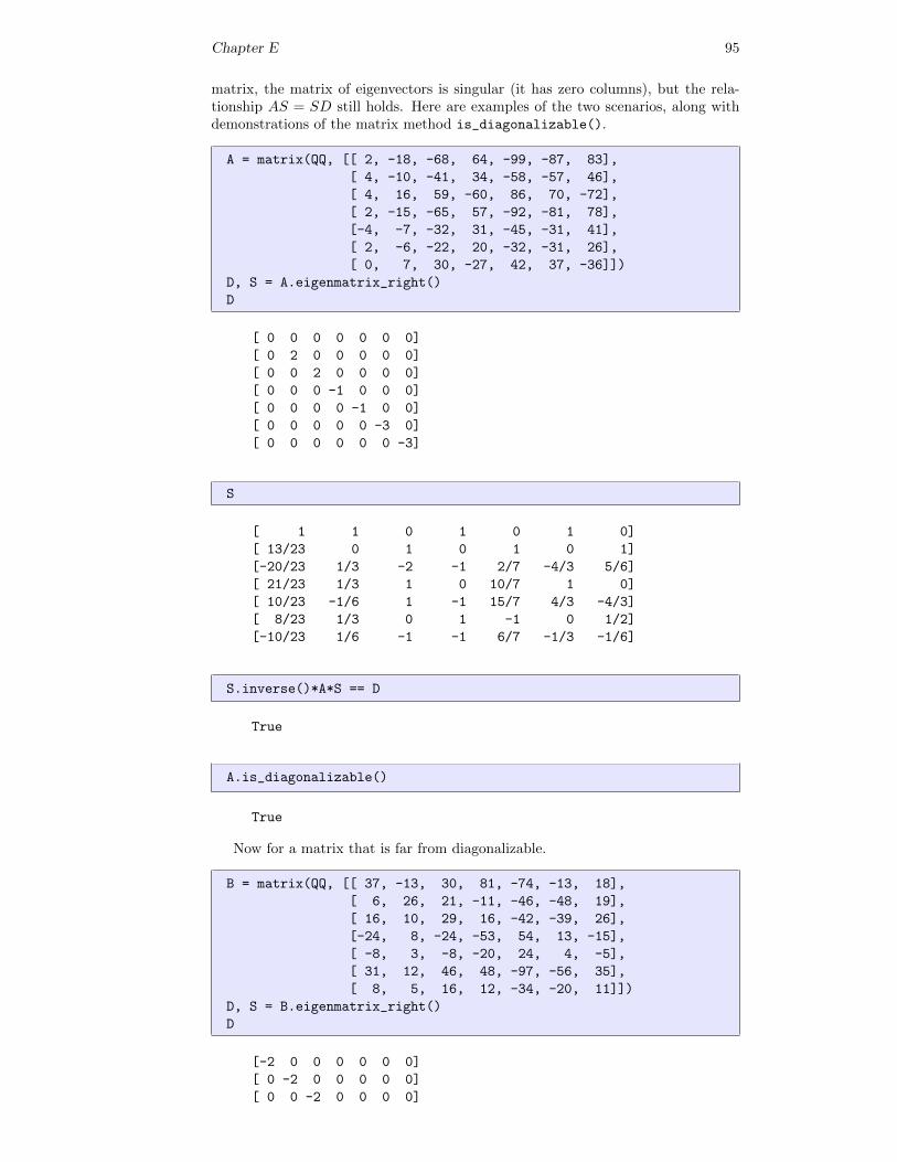
Chapter E 95
matrix, the matrix of eigenvectors is singular (it has zero columns), but the rela-tionship AS = SD still holds. Here are examples of the two scenarios, along withdemonstrations of the matrix method is_diagonalizable().
A = matrix(QQ, [[ 2, -18, -68, 64, -99, -87, 83],
[ 4, -10, -41, 34, -58, -57, 46],
[ 4, 16, 59, -60, 86, 70, -72],
[ 2, -15, -65, 57, -92, -81, 78],
[-4, -7, -32, 31, -45, -31, 41],
[ 2, -6, -22, 20, -32, -31, 26],
[ 0, 7, 30, -27, 42, 37, -36]])
D, S = A.eigenmatrix_right()
D
[ 0 0 0 0 0 0 0]
[ 0 2 0 0 0 0 0]
[ 0 0 2 0 0 0 0]
[ 0 0 0 -1 0 0 0]
[ 0 0 0 0 -1 0 0]
[ 0 0 0 0 0 -3 0]
[ 0 0 0 0 0 0 -3]
S
[ 1 1 0 1 0 1 0]
[ 13/23 0 1 0 1 0 1]
[-20/23 1/3 -2 -1 2/7 -4/3 5/6]
[ 21/23 1/3 1 0 10/7 1 0]
[ 10/23 -1/6 1 -1 15/7 4/3 -4/3]
[ 8/23 1/3 0 1 -1 0 1/2]
[-10/23 1/6 -1 -1 6/7 -1/3 -1/6]
S.inverse()*A*S == D
True
A.is_diagonalizable()
True
Now for a matrix that is far from diagonalizable.
B = matrix(QQ, [[ 37, -13, 30, 81, -74, -13, 18],
[ 6, 26, 21, -11, -46, -48, 19],
[ 16, 10, 29, 16, -42, -39, 26],
[-24, 8, -24, -53, 54, 13, -15],
[ -8, 3, -8, -20, 24, 4, -5],
[ 31, 12, 46, 48, -97, -56, 35],
[ 8, 5, 16, 12, -34, -20, 11]])
D, S = B.eigenmatrix_right()
D
[-2 0 0 0 0 0 0]
[ 0 -2 0 0 0 0 0]
[ 0 0 -2 0 0 0 0]
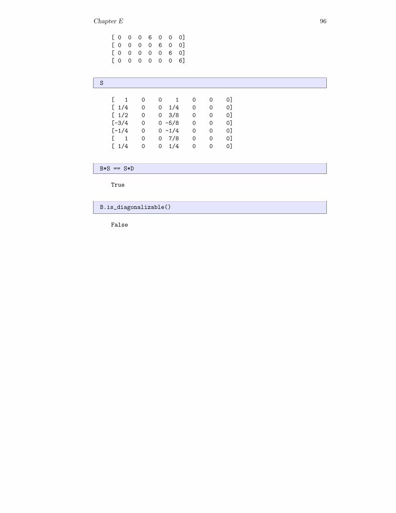
Chapter E 96
[ 0 0 0 6 0 0 0]
[ 0 0 0 0 6 0 0]
[ 0 0 0 0 0 6 0]
[ 0 0 0 0 0 0 6]
S
[ 1 0 0 1 0 0 0]
[ 1/4 0 0 1/4 0 0 0]
[ 1/2 0 0 3/8 0 0 0]
[-3/4 0 0 -5/8 0 0 0]
[-1/4 0 0 -1/4 0 0 0]
[ 1 0 0 7/8 0 0 0]
[ 1/4 0 0 1/4 0 0 0]
B*S == S*D
True
B.is_diagonalizable()
False
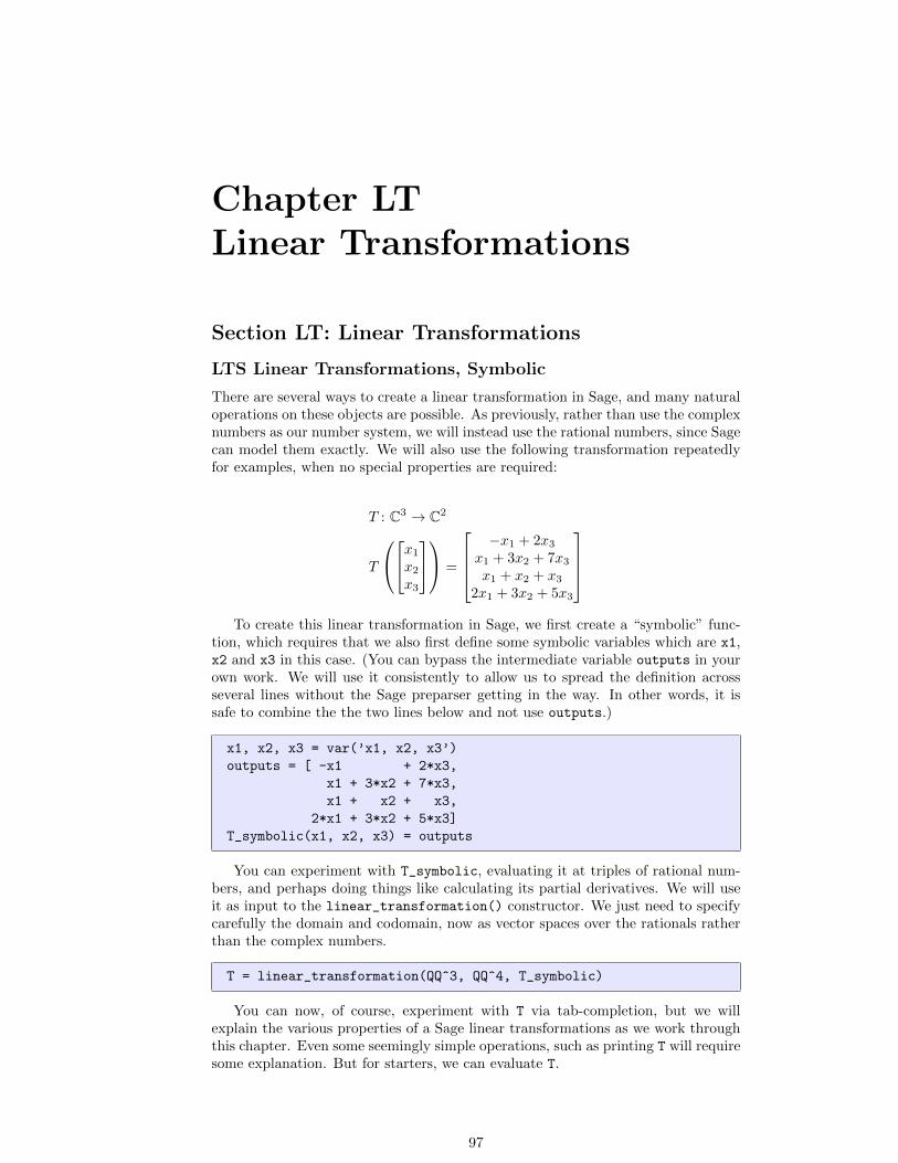
Chapter LTLinear Transformations
Section LT: Linear Transformations
LTS Linear Transformations, Symbolic
There are several ways to create a linear transformation in Sage, and many naturaloperations on these objects are possible. As previously, rather than use the complexnumbers as our number system, we will instead use the rational numbers, since Sagecan model them exactly. We will also use the following transformation repeatedlyfor examples, when no special properties are required:
T : C3 → C2
T
x1x2x3
=
−x1 + 2x3
x1 + 3x2 + 7x3x1 + x2 + x3
2x1 + 3x2 + 5x3
To create this linear transformation in Sage, we first create a “symbolic” func-
tion, which requires that we also first define some symbolic variables which are x1,x2 and x3 in this case. (You can bypass the intermediate variable outputs in yourown work. We will use it consistently to allow us to spread the definition acrossseveral lines without the Sage preparser getting in the way. In other words, it issafe to combine the the two lines below and not use outputs.)
x1, x2, x3 = var(’x1, x2, x3’)
outputs = [ -x1 + 2*x3,
x1 + 3*x2 + 7*x3,
x1 + x2 + x3,
2*x1 + 3*x2 + 5*x3]
T_symbolic(x1, x2, x3) = outputs
You can experiment with T_symbolic, evaluating it at triples of rational num-bers, and perhaps doing things like calculating its partial derivatives. We will useit as input to the linear_transformation() constructor. We just need to specifycarefully the domain and codomain, now as vector spaces over the rationals ratherthan the complex numbers.
T = linear_transformation(QQ^3, QQ^4, T_symbolic)
You can now, of course, experiment with T via tab-completion, but we willexplain the various properties of a Sage linear transformations as we work throughthis chapter. Even some seemingly simple operations, such as printing T will requiresome explanation. But for starters, we can evaluate T.
97
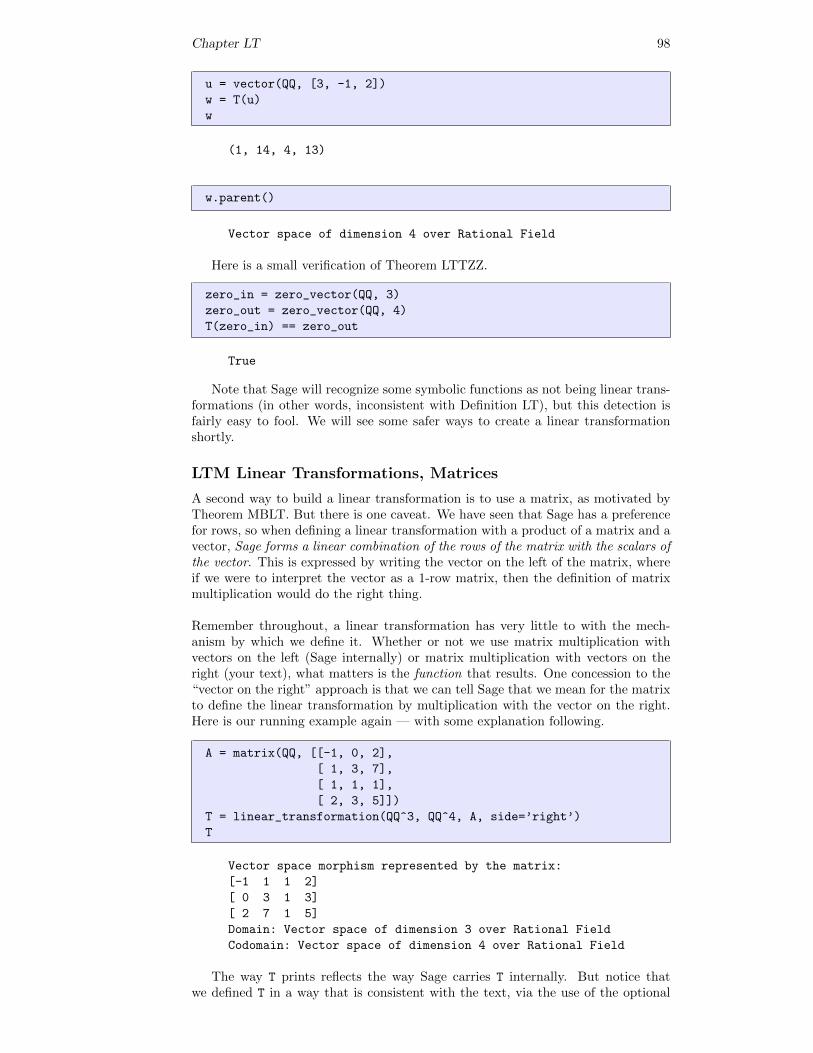
Chapter LT 98
u = vector(QQ, [3, -1, 2])
w = T(u)
w
(1, 14, 4, 13)
w.parent()
Vector space of dimension 4 over Rational Field
Here is a small verification of Theorem LTTZZ.
zero_in = zero_vector(QQ, 3)
zero_out = zero_vector(QQ, 4)
T(zero_in) == zero_out
True
Note that Sage will recognize some symbolic functions as not being linear trans-formations (in other words, inconsistent with Definition LT), but this detection isfairly easy to fool. We will see some safer ways to create a linear transformationshortly.
LTM Linear Transformations, Matrices
A second way to build a linear transformation is to use a matrix, as motivated byTheorem MBLT. But there is one caveat. We have seen that Sage has a preferencefor rows, so when defining a linear transformation with a product of a matrix and avector, Sage forms a linear combination of the rows of the matrix with the scalars ofthe vector. This is expressed by writing the vector on the left of the matrix, whereif we were to interpret the vector as a 1-row matrix, then the definition of matrixmultiplication would do the right thing.
Remember throughout, a linear transformation has very little to with the mech-anism by which we define it. Whether or not we use matrix multiplication withvectors on the left (Sage internally) or matrix multiplication with vectors on theright (your text), what matters is the function that results. One concession to the“vector on the right” approach is that we can tell Sage that we mean for the matrixto define the linear transformation by multiplication with the vector on the right.Here is our running example again — with some explanation following.
A = matrix(QQ, [[-1, 0, 2],
[ 1, 3, 7],
[ 1, 1, 1],
[ 2, 3, 5]])
T = linear_transformation(QQ^3, QQ^4, A, side=’right’)
T
Vector space morphism represented by the matrix:
[-1 1 1 2]
[ 0 3 1 3]
[ 2 7 1 5]
Domain: Vector space of dimension 3 over Rational Field
Codomain: Vector space of dimension 4 over Rational Field
The way T prints reflects the way Sage carries T internally. But notice thatwe defined T in a way that is consistent with the text, via the use of the optional
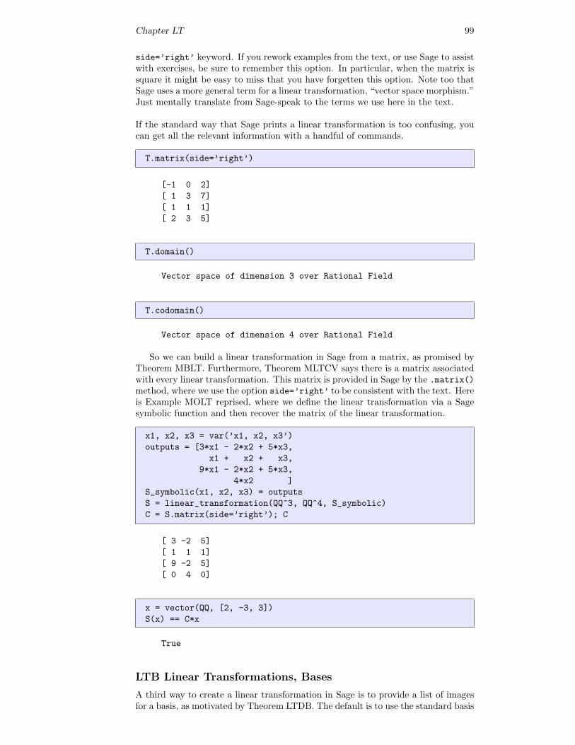
Chapter LT 99
side=’right’ keyword. If you rework examples from the text, or use Sage to assistwith exercises, be sure to remember this option. In particular, when the matrix issquare it might be easy to miss that you have forgetten this option. Note too thatSage uses a more general term for a linear transformation, “vector space morphism.”Just mentally translate from Sage-speak to the terms we use here in the text.
If the standard way that Sage prints a linear transformation is too confusing, youcan get all the relevant information with a handful of commands.
T.matrix(side=’right’)
[-1 0 2]
[ 1 3 7]
[ 1 1 1]
[ 2 3 5]
T.domain()
Vector space of dimension 3 over Rational Field
T.codomain()
Vector space of dimension 4 over Rational Field
So we can build a linear transformation in Sage from a matrix, as promised byTheorem MBLT. Furthermore, Theorem MLTCV says there is a matrix associatedwith every linear transformation. This matrix is provided in Sage by the .matrix()method, where we use the option side=’right’ to be consistent with the text. Hereis Example MOLT reprised, where we define the linear transformation via a Sagesymbolic function and then recover the matrix of the linear transformation.
x1, x2, x3 = var(’x1, x2, x3’)
outputs = [3*x1 - 2*x2 + 5*x3,
x1 + x2 + x3,
9*x1 - 2*x2 + 5*x3,
4*x2 ]
S_symbolic(x1, x2, x3) = outputs
S = linear_transformation(QQ^3, QQ^4, S_symbolic)
C = S.matrix(side=’right’); C
[ 3 -2 5]
[ 1 1 1]
[ 9 -2 5]
[ 0 4 0]
x = vector(QQ, [2, -3, 3])
S(x) == C*x
True
LTB Linear Transformations, Bases
A third way to create a linear transformation in Sage is to provide a list of imagesfor a basis, as motivated by Theorem LTDB. The default is to use the standard basis
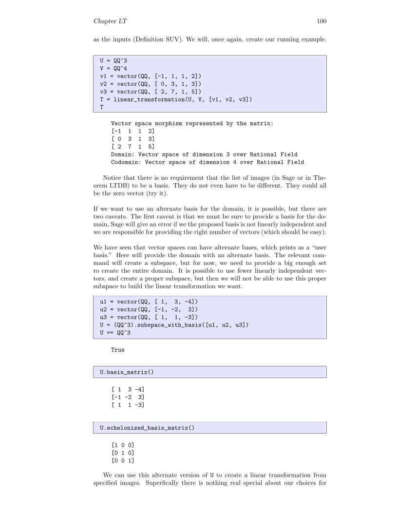
Chapter LT 100
as the inputs (Definition SUV). We will, once again, create our running example.
U = QQ^3
V = QQ^4
v1 = vector(QQ, [-1, 1, 1, 2])
v2 = vector(QQ, [ 0, 3, 1, 3])
v3 = vector(QQ, [ 2, 7, 1, 5])
T = linear_transformation(U, V, [v1, v2, v3])
T
Vector space morphism represented by the matrix:
[-1 1 1 2]
[ 0 3 1 3]
[ 2 7 1 5]
Domain: Vector space of dimension 3 over Rational Field
Codomain: Vector space of dimension 4 over Rational Field
Notice that there is no requirement that the list of images (in Sage or in The-orem LTDB) to be a basis. They do not even have to be different. They could allbe the zero vector (try it).
If we want to use an alternate basis for the domain, it is possible, but there aretwo caveats. The first caveat is that we must be sure to provide a basis for the do-main, Sage will give an error if we the proposed basis is not linearly independent andwe are responsible for providing the right number of vectors (which should be easy).
We have seen that vector spaces can have alternate bases, which prints as a “userbasis.” Here will provide the domain with an alternate basis. The relevant com-mand will create a subspace, but for now, we need to provide a big enough setto create the entire domain. It is possible to use fewer linearly independent vec-tors, and create a proper subspace, but then we will not be able to use this propersubspace to build the linear transformation we want.
u1 = vector(QQ, [ 1, 3, -4])
u2 = vector(QQ, [-1, -2, 3])
u3 = vector(QQ, [ 1, 1, -3])
U = (QQ^3).subspace_with_basis([u1, u2, u3])
U == QQ^3
True
U.basis_matrix()
[ 1 3 -4]
[-1 -2 3]
[ 1 1 -3]
U.echelonized_basis_matrix()
[1 0 0]
[0 1 0]
[0 0 1]
We can use this alternate version of U to create a linear transformation fromspecified images. Superfically there is nothing real special about our choices for
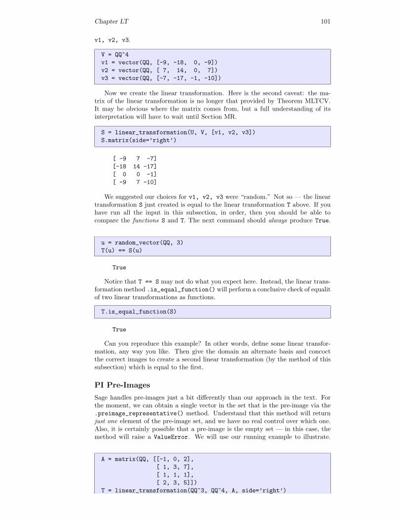
Chapter LT 101
v1, v2, v3.
V = QQ^4
v1 = vector(QQ, [-9, -18, 0, -9])
v2 = vector(QQ, [ 7, 14, 0, 7])
v3 = vector(QQ, [-7, -17, -1, -10])
Now we create the linear transformation. Here is the second caveat: the ma-trix of the linear transformation is no longer that provided by Theorem MLTCV.It may be obvious where the matrix comes from, but a full understanding of itsinterpretation will have to wait until Section MR.
S = linear_transformation(U, V, [v1, v2, v3])
S.matrix(side=’right’)
[ -9 7 -7]
[-18 14 -17]
[ 0 0 -1]
[ -9 7 -10]
We suggested our choices for v1, v2, v3 were “random.” Not so — the lineartransformation S just created is equal to the linear transformation T above. If youhave run all the input in this subsection, in order, then you should be able tocompare the functions S and T. The next command should always produce True.
u = random_vector(QQ, 3)
T(u) == S(u)
True
Notice that T == S may not do what you expect here. Instead, the linear trans-formation method .is_equal_function() will perform a conclusive check of equalitof two linear transformations as functions.
T.is_equal_function(S)
True
Can you reproduce this example? In other words, define some linear transfor-mation, any way you like. Then give the domain an alternate basis and concoctthe correct images to create a second linear transformation (by the method of thissubsection) which is equal to the first.
PI Pre-Images
Sage handles pre-images just a bit differently than our approach in the text. Forthe moment, we can obtain a single vector in the set that is the pre-image via the.preimage_representative() method. Understand that this method will returnjust one element of the pre-image set, and we have no real control over which one.Also, it is certainly possible that a pre-image is the empty set — in this case, themethod will raise a ValueError. We will use our running example to illustrate.
A = matrix(QQ, [[-1, 0, 2],
[ 1, 3, 7],
[ 1, 1, 1],
[ 2, 3, 5]])
T = linear_transformation(QQ^3, QQ^4, A, side=’right’)
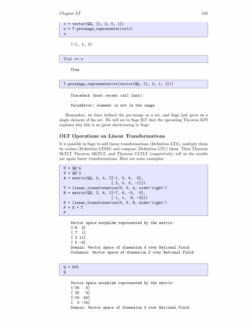
Chapter LT 102
v = vector(QQ, [1, 2, 0, 1])
u = T.preimage_representative(v)
u
(-1, 1, 0)
T(u) == v
True
T.preimage_representative(vector(QQ, [1, 2, 1, 1]))
Traceback (most recent call last):
...
ValueError: element is not in the image
Remember, we have defined the pre-image as a set, and Sage just gives us asingle element of the set. We will see in Sage ILT that the upcoming Theorem KPIexplains why this is no great shortcoming in Sage.
OLT Operations on Linear Transformations
It is possible in Sage to add linear transformations (Definition LTA), multiply themby scalars (Definition LTSM) and compose (Definition LTC) them. Then TheoremSLTLT Theorem MLTLT, and Theorem CLTLT (respectively) tell us the resultsare again linear transformations. Here are some examples:
U = QQ^4
V = QQ^2
A = matrix(QQ, 2, 4, [[-1, 3, 4, 5],
[ 2, 0, 3, -1]])
T = linear_transformation(U, V, A, side=’right’)
B = matrix(QQ, 2, 4, [[-7, 4, -2, 0],
[ 1, 1, 8, -3]])
S = linear_transformation(U, V, B, side=’right’)
P = S + T
P
Vector space morphism represented by the matrix:
[-8 3]
[ 7 1]
[ 2 11]
[ 5 -4]
Domain: Vector space of dimension 4 over Rational Field
Codomain: Vector space of dimension 2 over Rational Field
Q = S*5
Q
Vector space morphism represented by the matrix:
[-35 5]
[ 20 5]
[-10 40]
[ 0 -15]
Domain: Vector space of dimension 4 over Rational Field
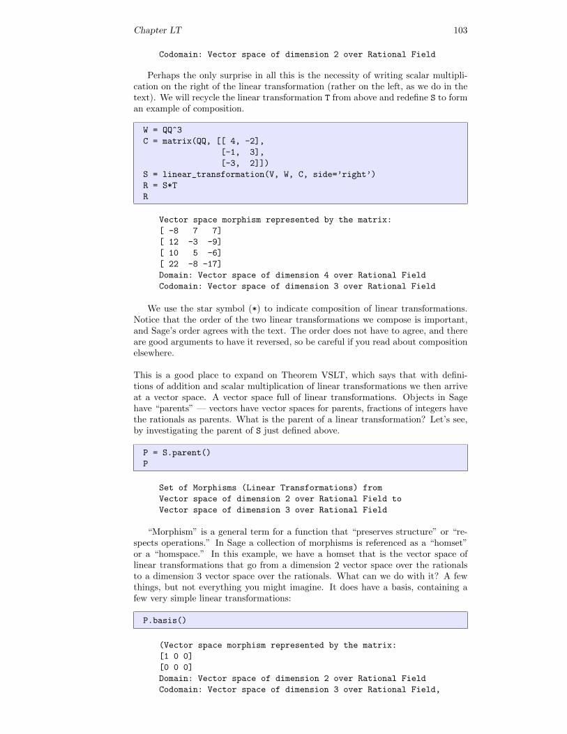
Chapter LT 103
Codomain: Vector space of dimension 2 over Rational Field
Perhaps the only surprise in all this is the necessity of writing scalar multipli-cation on the right of the linear transformation (rather on the left, as we do in thetext). We will recycle the linear transformation T from above and redefine S to forman example of composition.
W = QQ^3
C = matrix(QQ, [[ 4, -2],
[-1, 3],
[-3, 2]])
S = linear_transformation(V, W, C, side=’right’)
R = S*T
R
Vector space morphism represented by the matrix:
[ -8 7 7]
[ 12 -3 -9]
[ 10 5 -6]
[ 22 -8 -17]
Domain: Vector space of dimension 4 over Rational Field
Codomain: Vector space of dimension 3 over Rational Field
We use the star symbol (*) to indicate composition of linear transformations.Notice that the order of the two linear transformations we compose is important,and Sage’s order agrees with the text. The order does not have to agree, and thereare good arguments to have it reversed, so be careful if you read about compositionelsewhere.
This is a good place to expand on Theorem VSLT, which says that with defini-tions of addition and scalar multiplication of linear transformations we then arriveat a vector space. A vector space full of linear transformations. Objects in Sagehave “parents” — vectors have vector spaces for parents, fractions of integers havethe rationals as parents. What is the parent of a linear transformation? Let’s see,by investigating the parent of S just defined above.
P = S.parent()
P
Set of Morphisms (Linear Transformations) from
Vector space of dimension 2 over Rational Field to
Vector space of dimension 3 over Rational Field
“Morphism” is a general term for a function that “preserves structure” or “re-spects operations.” In Sage a collection of morphisms is referenced as a “homset”or a “homspace.” In this example, we have a homset that is the vector space oflinear transformations that go from a dimension 2 vector space over the rationalsto a dimension 3 vector space over the rationals. What can we do with it? A fewthings, but not everything you might imagine. It does have a basis, containing afew very simple linear transformations:
P.basis()
(Vector space morphism represented by the matrix:
[1 0 0]
[0 0 0]
Domain: Vector space of dimension 2 over Rational Field
Codomain: Vector space of dimension 3 over Rational Field,
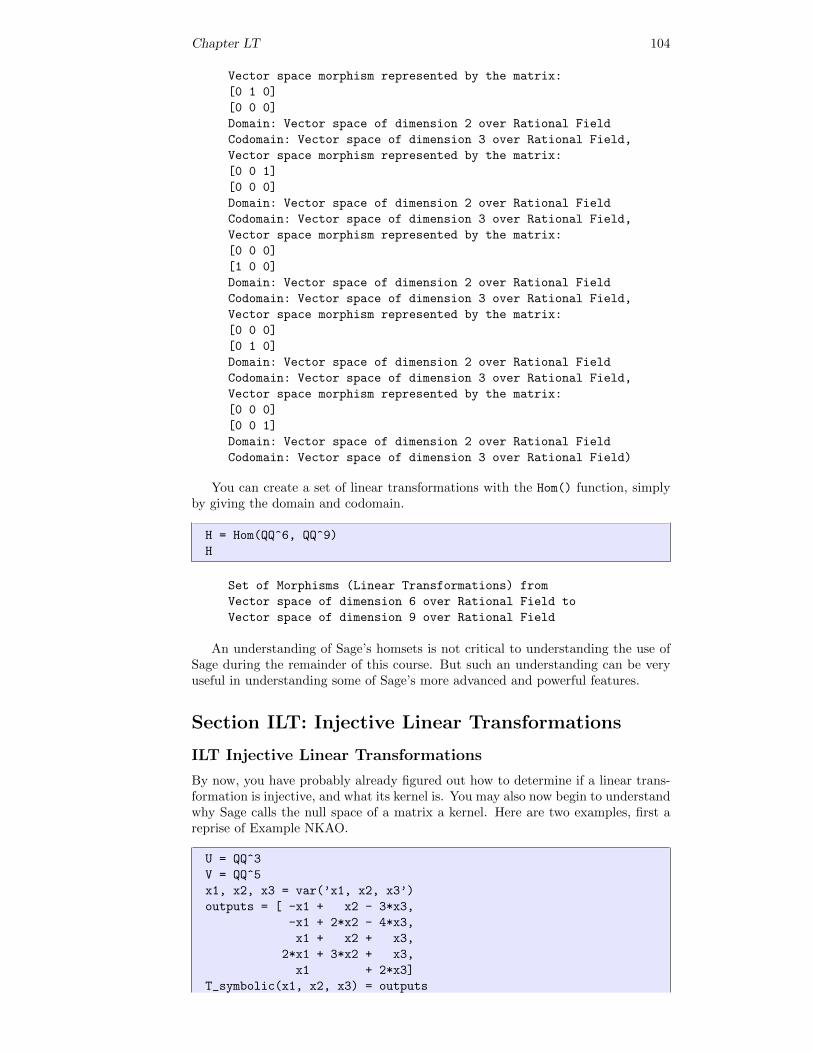
Chapter LT 104
Vector space morphism represented by the matrix:
[0 1 0]
[0 0 0]
Domain: Vector space of dimension 2 over Rational Field
Codomain: Vector space of dimension 3 over Rational Field,
Vector space morphism represented by the matrix:
[0 0 1]
[0 0 0]
Domain: Vector space of dimension 2 over Rational Field
Codomain: Vector space of dimension 3 over Rational Field,
Vector space morphism represented by the matrix:
[0 0 0]
[1 0 0]
Domain: Vector space of dimension 2 over Rational Field
Codomain: Vector space of dimension 3 over Rational Field,
Vector space morphism represented by the matrix:
[0 0 0]
[0 1 0]
Domain: Vector space of dimension 2 over Rational Field
Codomain: Vector space of dimension 3 over Rational Field,
Vector space morphism represented by the matrix:
[0 0 0]
[0 0 1]
Domain: Vector space of dimension 2 over Rational Field
Codomain: Vector space of dimension 3 over Rational Field)
You can create a set of linear transformations with the Hom() function, simplyby giving the domain and codomain.
H = Hom(QQ^6, QQ^9)
H
Set of Morphisms (Linear Transformations) from
Vector space of dimension 6 over Rational Field to
Vector space of dimension 9 over Rational Field
An understanding of Sage’s homsets is not critical to understanding the use ofSage during the remainder of this course. But such an understanding can be veryuseful in understanding some of Sage’s more advanced and powerful features.
Section ILT: Injective Linear Transformations
ILT Injective Linear Transformations
By now, you have probably already figured out how to determine if a linear trans-formation is injective, and what its kernel is. You may also now begin to understandwhy Sage calls the null space of a matrix a kernel. Here are two examples, first areprise of Example NKAO.
U = QQ^3
V = QQ^5
x1, x2, x3 = var(’x1, x2, x3’)
outputs = [ -x1 + x2 - 3*x3,
-x1 + 2*x2 - 4*x3,
x1 + x2 + x3,
2*x1 + 3*x2 + x3,
x1 + 2*x3]
T_symbolic(x1, x2, x3) = outputs
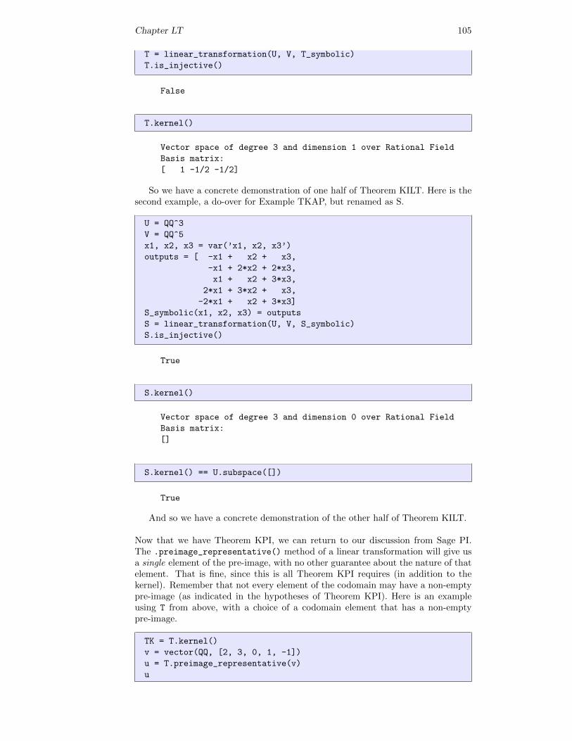
Chapter LT 105
T = linear_transformation(U, V, T_symbolic)
T.is_injective()
False
T.kernel()
Vector space of degree 3 and dimension 1 over Rational Field
Basis matrix:
[ 1 -1/2 -1/2]
So we have a concrete demonstration of one half of Theorem KILT. Here is thesecond example, a do-over for Example TKAP, but renamed as S.
U = QQ^3
V = QQ^5
x1, x2, x3 = var(’x1, x2, x3’)
outputs = [ -x1 + x2 + x3,
-x1 + 2*x2 + 2*x3,
x1 + x2 + 3*x3,
2*x1 + 3*x2 + x3,
-2*x1 + x2 + 3*x3]
S_symbolic(x1, x2, x3) = outputs
S = linear_transformation(U, V, S_symbolic)
S.is_injective()
True
S.kernel()
Vector space of degree 3 and dimension 0 over Rational Field
Basis matrix:
[]
S.kernel() == U.subspace([])
True
And so we have a concrete demonstration of the other half of Theorem KILT.
Now that we have Theorem KPI, we can return to our discussion from Sage PI.The .preimage_representative() method of a linear transformation will give usa single element of the pre-image, with no other guarantee about the nature of thatelement. That is fine, since this is all Theorem KPI requires (in addition to thekernel). Remember that not every element of the codomain may have a non-emptypre-image (as indicated in the hypotheses of Theorem KPI). Here is an exampleusing T from above, with a choice of a codomain element that has a non-emptypre-image.
TK = T.kernel()
v = vector(QQ, [2, 3, 0, 1, -1])
u = T.preimage_representative(v)
u
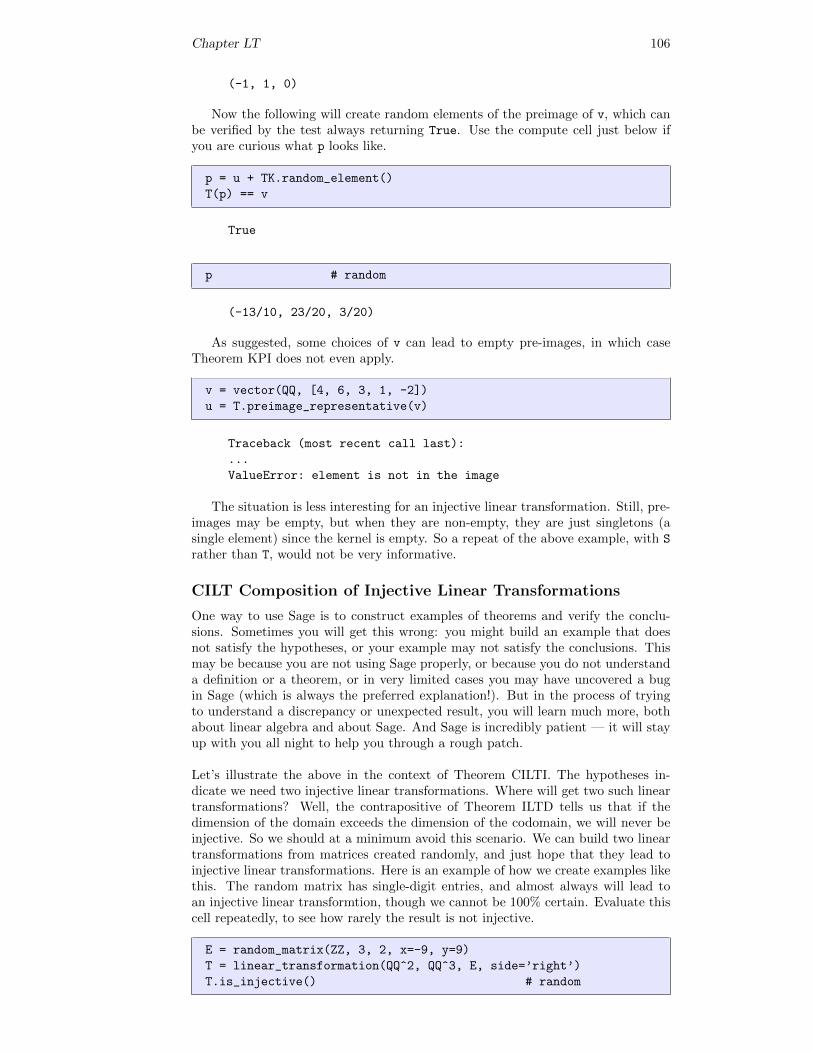
Chapter LT 106
(-1, 1, 0)
Now the following will create random elements of the preimage of v, which canbe verified by the test always returning True. Use the compute cell just below ifyou are curious what p looks like.
p = u + TK.random_element()
T(p) == v
True
p # random
(-13/10, 23/20, 3/20)
As suggested, some choices of v can lead to empty pre-images, in which caseTheorem KPI does not even apply.
v = vector(QQ, [4, 6, 3, 1, -2])
u = T.preimage_representative(v)
Traceback (most recent call last):
...
ValueError: element is not in the image
The situation is less interesting for an injective linear transformation. Still, pre-images may be empty, but when they are non-empty, they are just singletons (asingle element) since the kernel is empty. So a repeat of the above example, with S
rather than T, would not be very informative.
CILT Composition of Injective Linear Transformations
One way to use Sage is to construct examples of theorems and verify the conclu-sions. Sometimes you will get this wrong: you might build an example that doesnot satisfy the hypotheses, or your example may not satisfy the conclusions. Thismay be because you are not using Sage properly, or because you do not understanda definition or a theorem, or in very limited cases you may have uncovered a bugin Sage (which is always the preferred explanation!). But in the process of tryingto understand a discrepancy or unexpected result, you will learn much more, bothabout linear algebra and about Sage. And Sage is incredibly patient — it will stayup with you all night to help you through a rough patch.
Let’s illustrate the above in the context of Theorem CILTI. The hypotheses in-dicate we need two injective linear transformations. Where will get two such lineartransformations? Well, the contrapositive of Theorem ILTD tells us that if thedimension of the domain exceeds the dimension of the codomain, we will never beinjective. So we should at a minimum avoid this scenario. We can build two lineartransformations from matrices created randomly, and just hope that they lead toinjective linear transformations. Here is an example of how we create examples likethis. The random matrix has single-digit entries, and almost always will lead toan injective linear transformtion, though we cannot be 100% certain. Evaluate thiscell repeatedly, to see how rarely the result is not injective.
E = random_matrix(ZZ, 3, 2, x=-9, y=9)
T = linear_transformation(QQ^2, QQ^3, E, side=’right’)
T.is_injective() # random
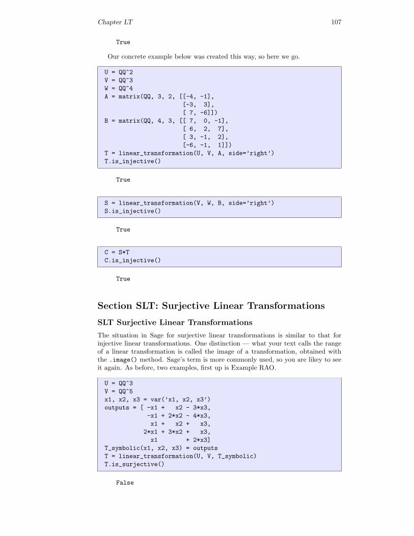
Chapter LT 107
True
Our concrete example below was created this way, so here we go.
U = QQ^2
V = QQ^3
W = QQ^4
A = matrix(QQ, 3, 2, [[-4, -1],
[-3, 3],
[ 7, -6]])
B = matrix(QQ, 4, 3, [[ 7, 0, -1],
[ 6, 2, 7],
[ 3, -1, 2],
[-6, -1, 1]])
T = linear_transformation(U, V, A, side=’right’)
T.is_injective()
True
S = linear_transformation(V, W, B, side=’right’)
S.is_injective()
True
C = S*T
C.is_injective()
True
Section SLT: Surjective Linear Transformations
SLT Surjective Linear Transformations
The situation in Sage for surjective linear transformations is similar to that forinjective linear transformations. One distinction — what your text calls the rangeof a linear transformation is called the image of a transformation, obtained withthe .image() method. Sage’s term is more commonly used, so you are likey to seeit again. As before, two examples, first up is Example RAO.
U = QQ^3
V = QQ^5
x1, x2, x3 = var(’x1, x2, x3’)
outputs = [ -x1 + x2 - 3*x3,
-x1 + 2*x2 - 4*x3,
x1 + x2 + x3,
2*x1 + 3*x2 + x3,
x1 + 2*x3]
T_symbolic(x1, x2, x3) = outputs
T = linear_transformation(U, V, T_symbolic)
T.is_surjective()
False
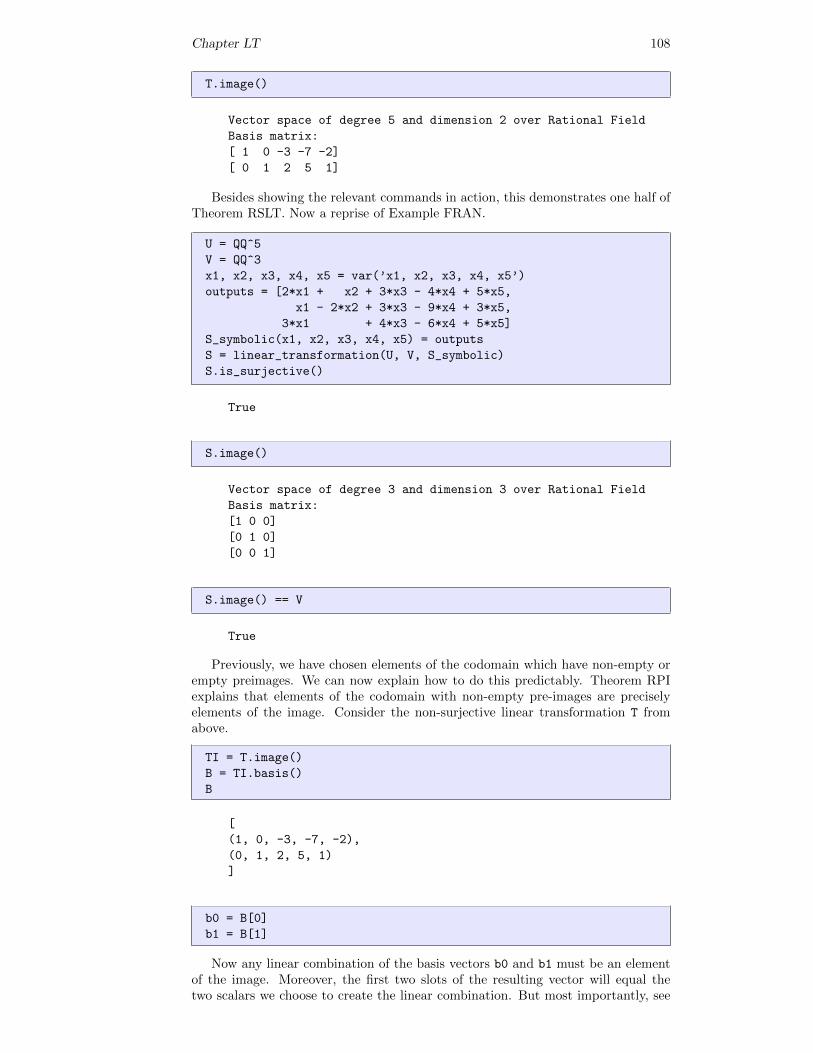
Chapter LT 108
T.image()
Vector space of degree 5 and dimension 2 over Rational Field
Basis matrix:
[ 1 0 -3 -7 -2]
[ 0 1 2 5 1]
Besides showing the relevant commands in action, this demonstrates one half ofTheorem RSLT. Now a reprise of Example FRAN.
U = QQ^5
V = QQ^3
x1, x2, x3, x4, x5 = var(’x1, x2, x3, x4, x5’)
outputs = [2*x1 + x2 + 3*x3 - 4*x4 + 5*x5,
x1 - 2*x2 + 3*x3 - 9*x4 + 3*x5,
3*x1 + 4*x3 - 6*x4 + 5*x5]
S_symbolic(x1, x2, x3, x4, x5) = outputs
S = linear_transformation(U, V, S_symbolic)
S.is_surjective()
True
S.image()
Vector space of degree 3 and dimension 3 over Rational Field
Basis matrix:
[1 0 0]
[0 1 0]
[0 0 1]
S.image() == V
True
Previously, we have chosen elements of the codomain which have non-empty orempty preimages. We can now explain how to do this predictably. Theorem RPIexplains that elements of the codomain with non-empty pre-images are preciselyelements of the image. Consider the non-surjective linear transformation T fromabove.
TI = T.image()
B = TI.basis()
B
[
(1, 0, -3, -7, -2),
(0, 1, 2, 5, 1)
]
b0 = B[0]
b1 = B[1]
Now any linear combination of the basis vectors b0 and b1 must be an elementof the image. Moreover, the first two slots of the resulting vector will equal thetwo scalars we choose to create the linear combination. But most importantly, see
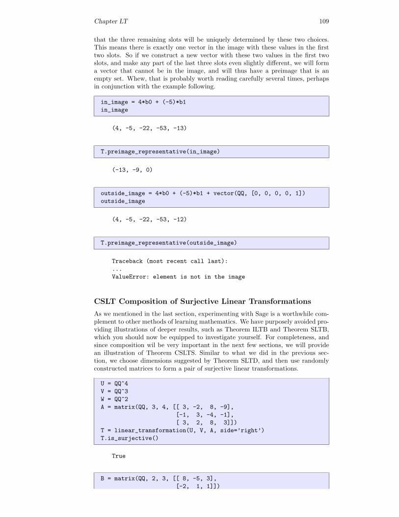
Chapter LT 109
that the three remaining slots will be uniquely determined by these two choices.This means there is exactly one vector in the image with these values in the firsttwo slots. So if we construct a new vector with these two values in the first twoslots, and make any part of the last three slots even slightly different, we will forma vector that cannot be in the image, and will thus have a preimage that is anempty set. Whew, that is probably worth reading carefully several times, perhapsin conjunction with the example following.
in_image = 4*b0 + (-5)*b1
in_image
(4, -5, -22, -53, -13)
T.preimage_representative(in_image)
(-13, -9, 0)
outside_image = 4*b0 + (-5)*b1 + vector(QQ, [0, 0, 0, 0, 1])
outside_image
(4, -5, -22, -53, -12)
T.preimage_representative(outside_image)
Traceback (most recent call last):
...
ValueError: element is not in the image
CSLT Composition of Surjective Linear Transformations
As we mentioned in the last section, experimenting with Sage is a worthwhile com-plement to other methods of learning mathematics. We have purposely avoided pro-viding illustrations of deeper results, such as Theorem ILTB and Theorem SLTB,which you should now be equipped to investigate yourself. For completeness, andsince composition wil be very important in the next few sections, we will providean illustration of Theorem CSLTS. Similar to what we did in the previous sec-tion, we choose dimensions suggested by Theorem SLTD, and then use randomlyconstructed matrices to form a pair of surjective linear transformations.
U = QQ^4
V = QQ^3
W = QQ^2
A = matrix(QQ, 3, 4, [[ 3, -2, 8, -9],
[-1, 3, -4, -1],
[ 3, 2, 8, 3]])
T = linear_transformation(U, V, A, side=’right’)
T.is_surjective()
True
B = matrix(QQ, 2, 3, [[ 8, -5, 3],
[-2, 1, 1]])
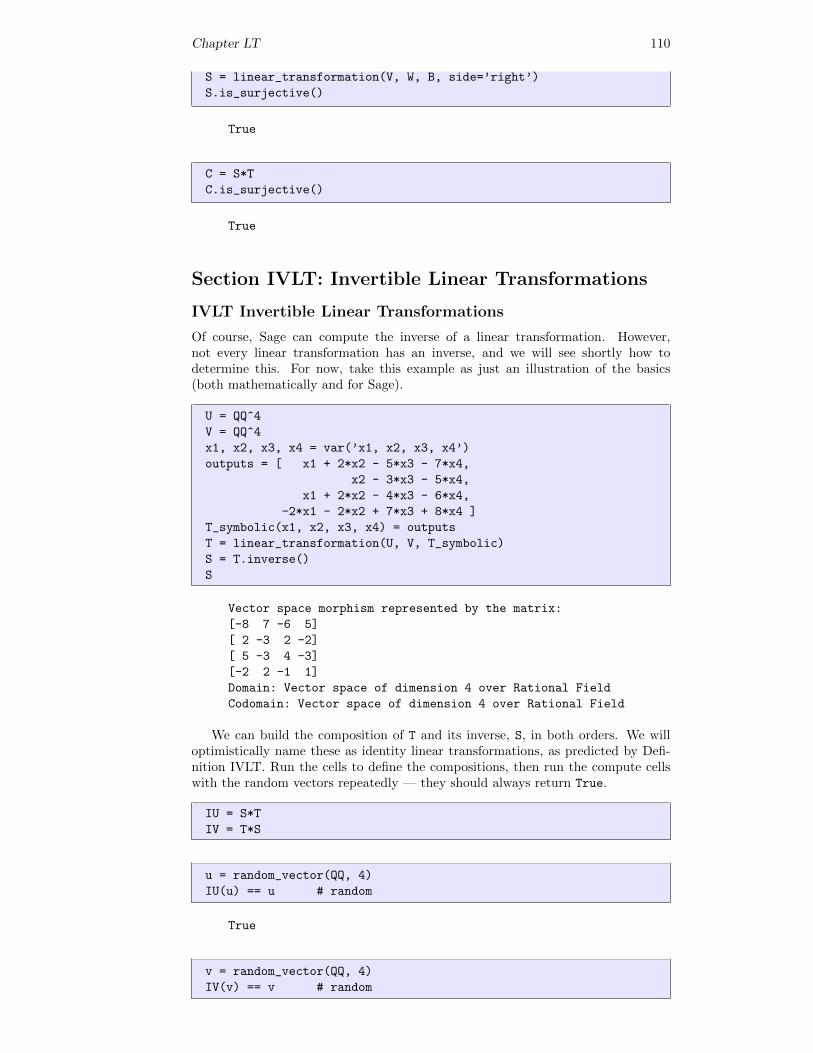
Chapter LT 110
S = linear_transformation(V, W, B, side=’right’)
S.is_surjective()
True
C = S*T
C.is_surjective()
True
Section IVLT: Invertible Linear Transformations
IVLT Invertible Linear Transformations
Of course, Sage can compute the inverse of a linear transformation. However,not every linear transformation has an inverse, and we will see shortly how todetermine this. For now, take this example as just an illustration of the basics(both mathematically and for Sage).
U = QQ^4
V = QQ^4
x1, x2, x3, x4 = var(’x1, x2, x3, x4’)
outputs = [ x1 + 2*x2 - 5*x3 - 7*x4,
x2 - 3*x3 - 5*x4,
x1 + 2*x2 - 4*x3 - 6*x4,
-2*x1 - 2*x2 + 7*x3 + 8*x4 ]
T_symbolic(x1, x2, x3, x4) = outputs
T = linear_transformation(U, V, T_symbolic)
S = T.inverse()
S
Vector space morphism represented by the matrix:
[-8 7 -6 5]
[ 2 -3 2 -2]
[ 5 -3 4 -3]
[-2 2 -1 1]
Domain: Vector space of dimension 4 over Rational Field
Codomain: Vector space of dimension 4 over Rational Field
We can build the composition of T and its inverse, S, in both orders. We willoptimistically name these as identity linear transformations, as predicted by Defi-nition IVLT. Run the cells to define the compositions, then run the compute cellswith the random vectors repeatedly — they should always return True.
IU = S*T
IV = T*S
u = random_vector(QQ, 4)
IU(u) == u # random
True
v = random_vector(QQ, 4)
IV(v) == v # random
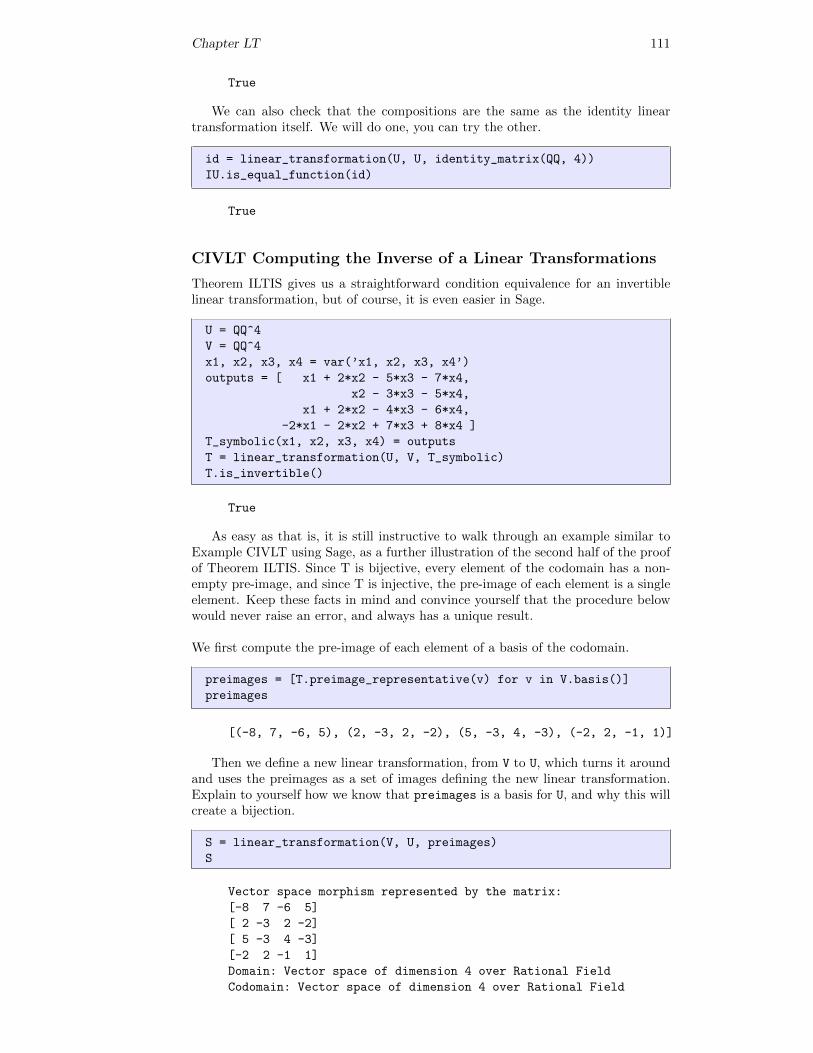
Chapter LT 111
True
We can also check that the compositions are the same as the identity lineartransformation itself. We will do one, you can try the other.
id = linear_transformation(U, U, identity_matrix(QQ, 4))
IU.is_equal_function(id)
True
CIVLT Computing the Inverse of a Linear Transformations
Theorem ILTIS gives us a straightforward condition equivalence for an invertiblelinear transformation, but of course, it is even easier in Sage.
U = QQ^4
V = QQ^4
x1, x2, x3, x4 = var(’x1, x2, x3, x4’)
outputs = [ x1 + 2*x2 - 5*x3 - 7*x4,
x2 - 3*x3 - 5*x4,
x1 + 2*x2 - 4*x3 - 6*x4,
-2*x1 - 2*x2 + 7*x3 + 8*x4 ]
T_symbolic(x1, x2, x3, x4) = outputs
T = linear_transformation(U, V, T_symbolic)
T.is_invertible()
True
As easy as that is, it is still instructive to walk through an example similar toExample CIVLT using Sage, as a further illustration of the second half of the proofof Theorem ILTIS. Since T is bijective, every element of the codomain has a non-empty pre-image, and since T is injective, the pre-image of each element is a singleelement. Keep these facts in mind and convince yourself that the procedure belowwould never raise an error, and always has a unique result.
We first compute the pre-image of each element of a basis of the codomain.
preimages = [T.preimage_representative(v) for v in V.basis()]
preimages
[(-8, 7, -6, 5), (2, -3, 2, -2), (5, -3, 4, -3), (-2, 2, -1, 1)]
Then we define a new linear transformation, from V to U, which turns it aroundand uses the preimages as a set of images defining the new linear transformation.Explain to yourself how we know that preimages is a basis for U, and why this willcreate a bijection.
S = linear_transformation(V, U, preimages)
S
Vector space morphism represented by the matrix:
[-8 7 -6 5]
[ 2 -3 2 -2]
[ 5 -3 4 -3]
[-2 2 -1 1]
Domain: Vector space of dimension 4 over Rational Field
Codomain: Vector space of dimension 4 over Rational Field
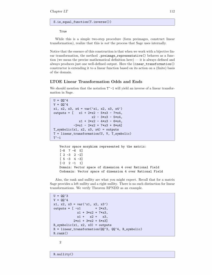
Chapter LT 112
S.is_equal_function(T.inverse())
True
While this is a simple two-step procedure (form preimages, construct lineartransformation), realize that this is not the process that Sage uses internally.
Notice that the essence of this construction is that when we work with a bijective lin-ear transformation, the method .preimage_representative() behaves as a func-tion (we mean the precise mathematical definition here) — it is always defined andalways produces just one well-defined output. Here the linear_transformation()
constructor is extending it to a linear function based on its action on a (finite) basisof the domain.
LTOE Linear Transformation Odds and Ends
We should mention that the notation T^-1 will yield an inverse of a linear transfor-mation in Sage.
U = QQ^4
V = QQ^4
x1, x2, x3, x4 = var(’x1, x2, x3, x4’)
outputs = [ x1 + 2*x2 - 5*x3 - 7*x4,
x2 - 3*x3 - 5*x4,
x1 + 2*x2 - 4*x3 - 6*x4,
-2*x1 - 2*x2 + 7*x3 + 8*x4]
T_symbolic(x1, x2, x3, x4) = outputs
T = linear_transformation(U, V, T_symbolic)
T^-1
Vector space morphism represented by the matrix:
[-8 7 -6 5]
[ 2 -3 2 -2]
[ 5 -3 4 -3]
[-2 2 -1 1]
Domain: Vector space of dimension 4 over Rational Field
Codomain: Vector space of dimension 4 over Rational Field
Also, the rank and nullity are what you might expect. Recall that for a matrixSage provides a left nullity and a right nullity. There is no such distinction for lineartransformations. We verify Theorem RPNDD as an example.
U = QQ^3
V = QQ^4
x1, x2, x3 = var(’x1, x2, x3’)
outputs = [ -x1 + 2*x3,
x1 + 3*x2 + 7*x3,
x1 + x2 + x3,
2*x1 + 3*x2 + 5*x3]
R_symbolic(x1, x2, x3) = outputs
R = linear_transformation(QQ^3, QQ^4, R_symbolic)
R.rank()
2
R.nullity()
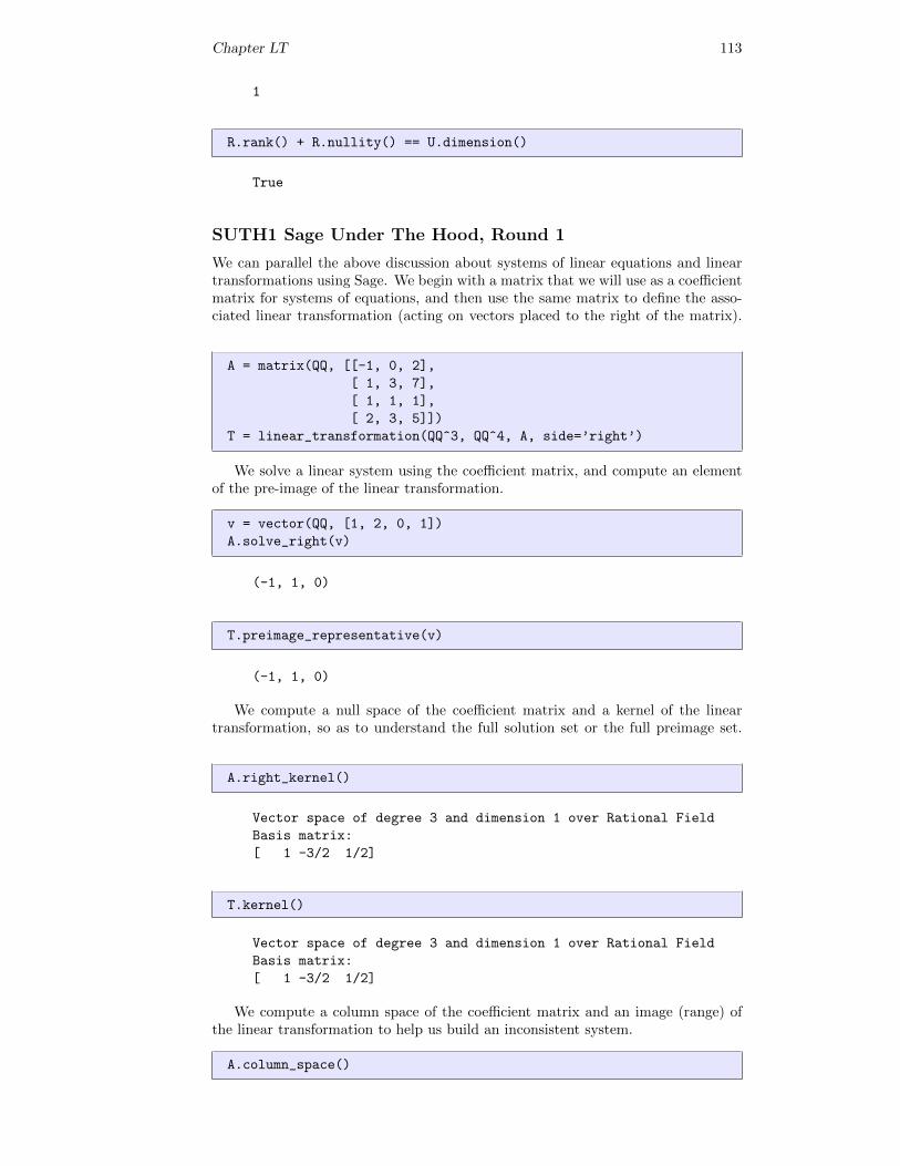
Chapter LT 113
1
R.rank() + R.nullity() == U.dimension()
True
SUTH1 Sage Under The Hood, Round 1
We can parallel the above discussion about systems of linear equations and lineartransformations using Sage. We begin with a matrix that we will use as a coefficientmatrix for systems of equations, and then use the same matrix to define the asso-ciated linear transformation (acting on vectors placed to the right of the matrix).
A = matrix(QQ, [[-1, 0, 2],
[ 1, 3, 7],
[ 1, 1, 1],
[ 2, 3, 5]])
T = linear_transformation(QQ^3, QQ^4, A, side=’right’)
We solve a linear system using the coefficient matrix, and compute an elementof the pre-image of the linear transformation.
v = vector(QQ, [1, 2, 0, 1])
A.solve_right(v)
(-1, 1, 0)
T.preimage_representative(v)
(-1, 1, 0)
We compute a null space of the coefficient matrix and a kernel of the lineartransformation, so as to understand the full solution set or the full preimage set.
A.right_kernel()
Vector space of degree 3 and dimension 1 over Rational Field
Basis matrix:
[ 1 -3/2 1/2]
T.kernel()
Vector space of degree 3 and dimension 1 over Rational Field
Basis matrix:
[ 1 -3/2 1/2]
We compute a column space of the coefficient matrix and an image (range) ofthe linear transformation to help us build an inconsistent system.
A.column_space()
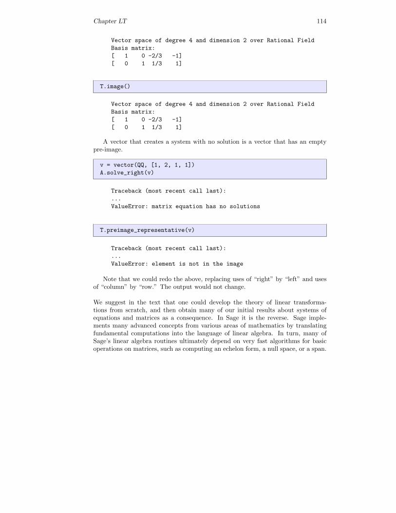
Chapter LT 114
Vector space of degree 4 and dimension 2 over Rational Field
Basis matrix:
[ 1 0 -2/3 -1]
[ 0 1 1/3 1]
T.image()
Vector space of degree 4 and dimension 2 over Rational Field
Basis matrix:
[ 1 0 -2/3 -1]
[ 0 1 1/3 1]
A vector that creates a system with no solution is a vector that has an emptypre-image.
v = vector(QQ, [1, 2, 1, 1])
A.solve_right(v)
Traceback (most recent call last):
...
ValueError: matrix equation has no solutions
T.preimage_representative(v)
Traceback (most recent call last):
...
ValueError: element is not in the image
Note that we could redo the above, replacing uses of “right” by “left” and usesof “column” by “row.” The output would not change.
We suggest in the text that one could develop the theory of linear transforma-tions from scratch, and then obtain many of our initial results about systems ofequations and matrices as a consequence. In Sage it is the reverse. Sage imple-ments many advanced concepts from various areas of mathematics by translatingfundamental computations into the language of linear algebra. In turn, many ofSage’s linear algebra routines ultimately depend on very fast algorithms for basicoperations on matrices, such as computing an echelon form, a null space, or a span.
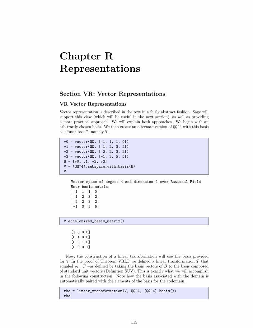
Chapter RRepresentations
Section VR: Vector Representations
VR Vector Representations
Vector representation is described in the text in a fairly abstract fashion. Sage willsupport this view (which will be useful in the next section), as well as providinga more practical approach. We will explain both approaches. We begin with anarbitrarily chosen basis. We then create an alternate version of QQ^4 with this basisas a“user basis”, namely V.
v0 = vector(QQ, [ 1, 1, 1, 0])
v1 = vector(QQ, [ 1, 2, 3, 2])
v2 = vector(QQ, [ 2, 2, 3, 2])
v3 = vector(QQ, [-1, 3, 5, 5])
B = [v0, v1, v2, v3]
V = (QQ^4).subspace_with_basis(B)
V
Vector space of degree 4 and dimension 4 over Rational Field
User basis matrix:
[ 1 1 1 0]
[ 1 2 3 2]
[ 2 2 3 2]
[-1 3 5 5]
V.echelonized_basis_matrix()
[1 0 0 0]
[0 1 0 0]
[0 0 1 0]
[0 0 0 1]
Now, the construction of a linear transformation will use the basis providedfor V. In the proof of Theorem VRLT we defined a linear transformation T thatequaled ρB . T was defined by taking the basis vectors of B to the basis composedof standard unit vectors (Definition SUV). This is exactly what we will accomplishin the following construction. Note how the basis associated with the domain isautomatically paired with the elements of the basis for the codomain.
rho = linear_transformation(V, QQ^4, (QQ^4).basis())
rho
115
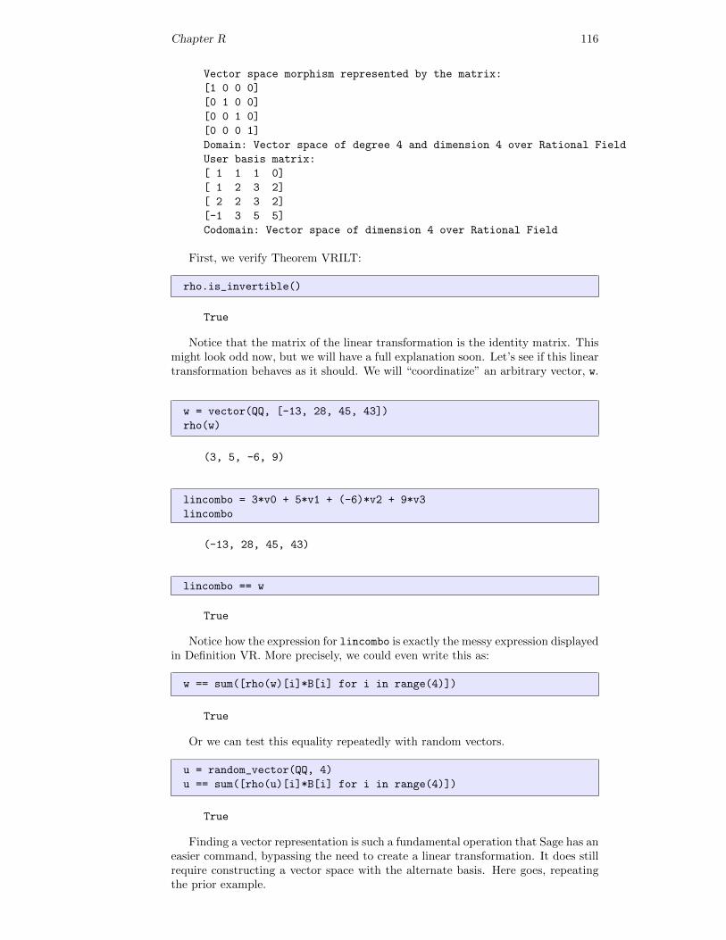
Chapter R 116
Vector space morphism represented by the matrix:
[1 0 0 0]
[0 1 0 0]
[0 0 1 0]
[0 0 0 1]
Domain: Vector space of degree 4 and dimension 4 over Rational Field
User basis matrix:
[ 1 1 1 0]
[ 1 2 3 2]
[ 2 2 3 2]
[-1 3 5 5]
Codomain: Vector space of dimension 4 over Rational Field
First, we verify Theorem VRILT:
rho.is_invertible()
True
Notice that the matrix of the linear transformation is the identity matrix. Thismight look odd now, but we will have a full explanation soon. Let’s see if this lineartransformation behaves as it should. We will “coordinatize” an arbitrary vector, w.
w = vector(QQ, [-13, 28, 45, 43])
rho(w)
(3, 5, -6, 9)
lincombo = 3*v0 + 5*v1 + (-6)*v2 + 9*v3
lincombo
(-13, 28, 45, 43)
lincombo == w
True
Notice how the expression for lincombo is exactly the messy expression displayedin Definition VR. More precisely, we could even write this as:
w == sum([rho(w)[i]*B[i] for i in range(4)])
True
Or we can test this equality repeatedly with random vectors.
u = random_vector(QQ, 4)
u == sum([rho(u)[i]*B[i] for i in range(4)])
True
Finding a vector representation is such a fundamental operation that Sage has aneasier command, bypassing the need to create a linear transformation. It does stillrequire constructing a vector space with the alternate basis. Here goes, repeatingthe prior example.
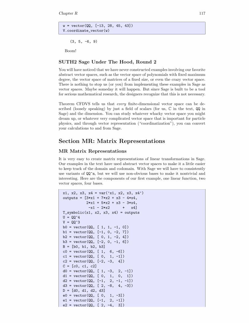
Chapter R 117
w = vector(QQ, [-13, 28, 45, 43])
V.coordinate_vector(w)
(3, 5, -6, 9)
Boom!
SUTH2 Sage Under The Hood, Round 2
You will have noticed that we have never constructed examples involving our favoriteabstract vector spaces, such as the vector space of polynomials with fixed maximumdegree, the vector space of matrices of a fixed size, or even the crazy vector space.There is nothing to stop us (or you) from implementing these examples in Sage asvector spaces. Maybe someday it will happen. But since Sage is built to be a toolfor serious mathematical research, the designers recognize that this is not necessary.
Theorem CFDVS tells us that every finite-dimensional vector space can be de-scribed (loosely speaking) by just a field of scalars (for us, C in the text, QQ inSage) and the dimension. You can study whatever whacky vector space you mightdream up, or whatever very complicated vector space that is important for particlephysics, and through vector representation (“coordinatization”), you can convertyour calculations to and from Sage.
Section MR: Matrix Representations
MR Matrix Representations
It is very easy to create matrix representations of linear transformations in Sage.Our examples in the text have used abstract vector spaces to make it a little easierto keep track of the domain and codomain. With Sage we will have to consistentlyuse variants of QQ^n, but we will use non-obvious bases to make it nontrivial andinteresting. Here are the components of our first example, one linear function, twovector spaces, four bases.
x1, x2, x3, x4 = var(’x1, x2, x3, x4’)
outputs = [3*x1 + 7*x2 + x3 - 4*x4,
2*x1 + 5*x2 + x3 - 3*x4,
-x1 - 2*x2 + x4]
T_symbolic(x1, x2, x3, x4) = outputs
U = QQ^4
V = QQ^3
b0 = vector(QQ, [ 1, 1, -1, 0])
b1 = vector(QQ, [-1, 0, -2, 7])
b2 = vector(QQ, [ 0, 1, -2, 4])
b3 = vector(QQ, [-2, 0, -1, 6])
B = [b0, b1, b2, b3]
c0 = vector(QQ, [ 1, 6, -6])
c1 = vector(QQ, [ 0, 1, -1])
c2 = vector(QQ, [-2, -3, 4])
C = [c0, c1, c2]
d0 = vector(QQ, [ 1, -3, 2, -1])
d1 = vector(QQ, [ 0, 1, 0, 1])
d2 = vector(QQ, [-1, 2, -1, -1])
d3 = vector(QQ, [ 2, -8, 4, -3])
D = [d0, d1, d2, d3]
e0 = vector(QQ, [ 0, 1, -3])
e1 = vector(QQ, [-1, 2, -1])
e2 = vector(QQ, [ 2, -4, 3])
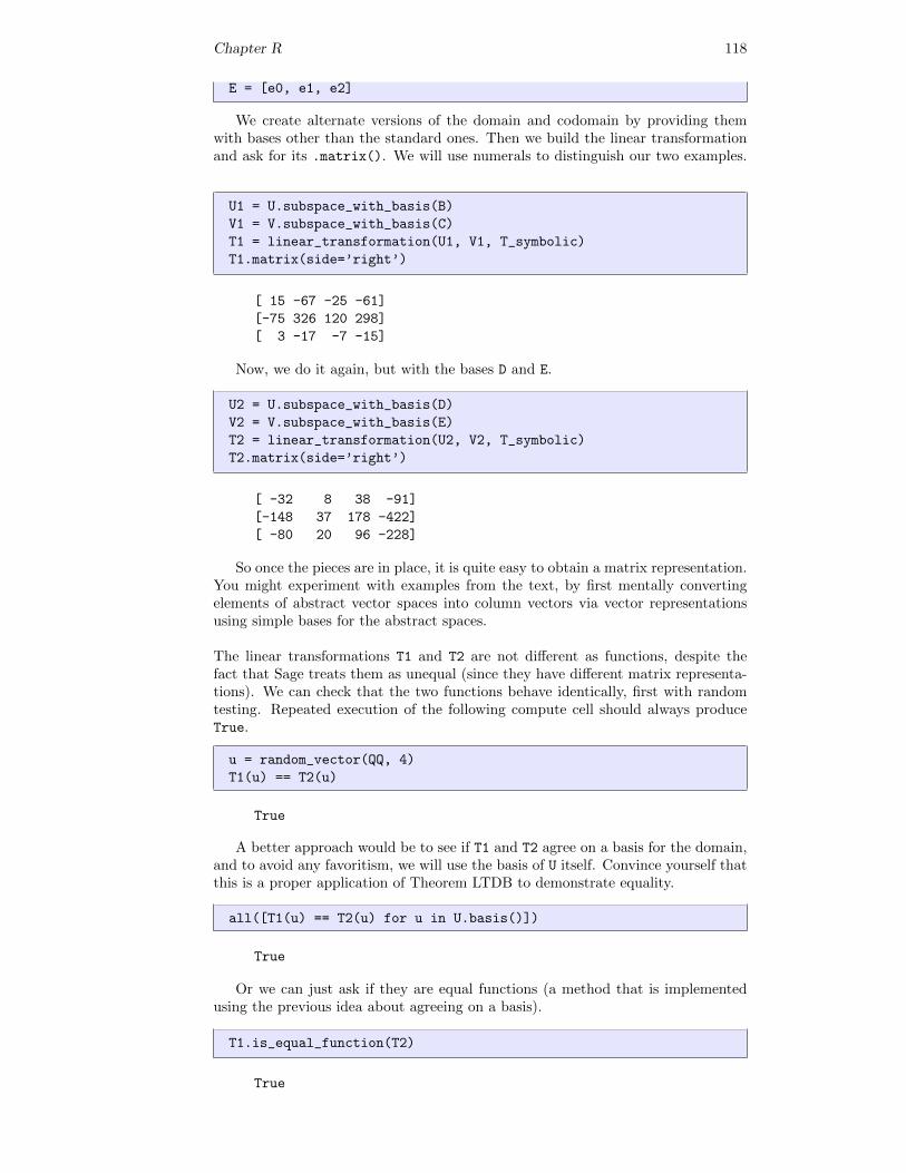
Chapter R 118
E = [e0, e1, e2]
We create alternate versions of the domain and codomain by providing themwith bases other than the standard ones. Then we build the linear transformationand ask for its .matrix(). We will use numerals to distinguish our two examples.
U1 = U.subspace_with_basis(B)
V1 = V.subspace_with_basis(C)
T1 = linear_transformation(U1, V1, T_symbolic)
T1.matrix(side=’right’)
[ 15 -67 -25 -61]
[-75 326 120 298]
[ 3 -17 -7 -15]
Now, we do it again, but with the bases D and E.
U2 = U.subspace_with_basis(D)
V2 = V.subspace_with_basis(E)
T2 = linear_transformation(U2, V2, T_symbolic)
T2.matrix(side=’right’)
[ -32 8 38 -91]
[-148 37 178 -422]
[ -80 20 96 -228]
So once the pieces are in place, it is quite easy to obtain a matrix representation.You might experiment with examples from the text, by first mentally convertingelements of abstract vector spaces into column vectors via vector representationsusing simple bases for the abstract spaces.
The linear transformations T1 and T2 are not different as functions, despite thefact that Sage treats them as unequal (since they have different matrix representa-tions). We can check that the two functions behave identically, first with randomtesting. Repeated execution of the following compute cell should always produceTrue.
u = random_vector(QQ, 4)
T1(u) == T2(u)
True
A better approach would be to see if T1 and T2 agree on a basis for the domain,and to avoid any favoritism, we will use the basis of U itself. Convince yourself thatthis is a proper application of Theorem LTDB to demonstrate equality.
all([T1(u) == T2(u) for u in U.basis()])
True
Or we can just ask if they are equal functions (a method that is implementedusing the previous idea about agreeing on a basis).
T1.is_equal_function(T2)
True
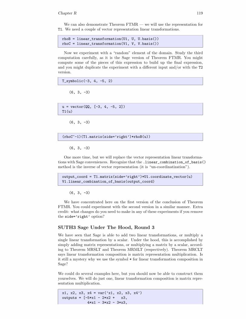
Chapter R 119
We can also demonstrate Theorem FTMR — we will use the representation forT1. We need a couple of vector representation linear transformations.
rhoB = linear_transformation(U1, U, U.basis())
rhoC = linear_transformation(V1, V, V.basis())
Now we experiment with a “random” element of the domain. Study the thirdcomputation carefully, as it is the Sage version of Theorem FTMR. You mightcompute some of the pieces of this expression to build up the final expression,and you might duplicate the experiment with a different input and/or with the T2
version.
T_symbolic(-3, 4, -5, 2)
(6, 3, -3)
u = vector(QQ, [-3, 4, -5, 2])
T1(u)
(6, 3, -3)
(rhoC^-1)(T1.matrix(side=’right’)*rhoB(u))
(6, 3, -3)
One more time, but we will replace the vector representation linear transforma-tions with Sage conveniences. Recognize that the .linear_combination_of_basis()method is the inverse of vector representation (it is “un-coordinatization”).
output_coord = T1.matrix(side=’right’)*U1.coordinate_vector(u)
V1.linear_combination_of_basis(output_coord)
(6, 3, -3)
We have concentrated here on the first version of the conclusion of TheoremFTMR. You could experiment with the second version in a similar manner. Extracredit: what changes do you need to make in any of these experiments if you removethe side=’right’ option?
SUTH3 Sage Under The Hood, Round 3
We have seen that Sage is able to add two linear transformations, or multiply asingle linear transformation by a scalar. Under the hood, this is accomplished bysimply adding matrix representations, or multiplying a matrix by a scalar, accord-ing to Theorem MRSLT and Theorem MRMLT (respectively). Theorem MRCLTsays linear transformation composition is matrix representation multiplication. Isit still a mystery why we use the symbol * for linear transformation composition inSage?
We could do several examples here, but you should now be able to construct themyourselves. We will do just one, linear transformation composition is matrix repre-sentation multiplication.
x1, x2, x3, x4 = var(’x1, x2, x3, x4’)
outputs = [-5*x1 - 2*x2 + x3,
4*x1 - 3*x2 - 3*x3,
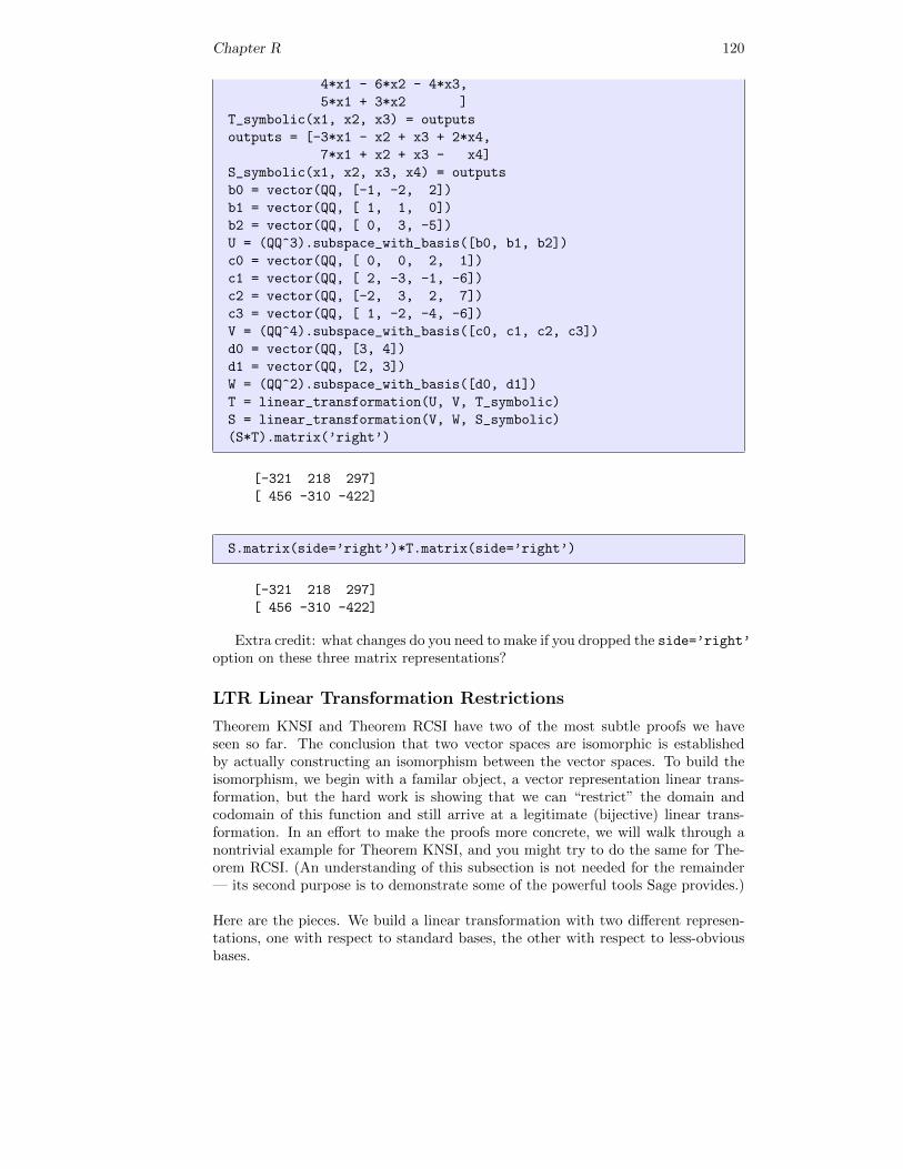
Chapter R 120
4*x1 - 6*x2 - 4*x3,
5*x1 + 3*x2 ]
T_symbolic(x1, x2, x3) = outputs
outputs = [-3*x1 - x2 + x3 + 2*x4,
7*x1 + x2 + x3 - x4]
S_symbolic(x1, x2, x3, x4) = outputs
b0 = vector(QQ, [-1, -2, 2])
b1 = vector(QQ, [ 1, 1, 0])
b2 = vector(QQ, [ 0, 3, -5])
U = (QQ^3).subspace_with_basis([b0, b1, b2])
c0 = vector(QQ, [ 0, 0, 2, 1])
c1 = vector(QQ, [ 2, -3, -1, -6])
c2 = vector(QQ, [-2, 3, 2, 7])
c3 = vector(QQ, [ 1, -2, -4, -6])
V = (QQ^4).subspace_with_basis([c0, c1, c2, c3])
d0 = vector(QQ, [3, 4])
d1 = vector(QQ, [2, 3])
W = (QQ^2).subspace_with_basis([d0, d1])
T = linear_transformation(U, V, T_symbolic)
S = linear_transformation(V, W, S_symbolic)
(S*T).matrix(’right’)
[-321 218 297]
[ 456 -310 -422]
S.matrix(side=’right’)*T.matrix(side=’right’)
[-321 218 297]
[ 456 -310 -422]
Extra credit: what changes do you need to make if you dropped the side=’right’option on these three matrix representations?
LTR Linear Transformation Restrictions
Theorem KNSI and Theorem RCSI have two of the most subtle proofs we haveseen so far. The conclusion that two vector spaces are isomorphic is establishedby actually constructing an isomorphism between the vector spaces. To build theisomorphism, we begin with a familar object, a vector representation linear trans-formation, but the hard work is showing that we can “restrict” the domain andcodomain of this function and still arrive at a legitimate (bijective) linear trans-formation. In an effort to make the proofs more concrete, we will walk through anontrivial example for Theorem KNSI, and you might try to do the same for The-orem RCSI. (An understanding of this subsection is not needed for the remainder— its second purpose is to demonstrate some of the powerful tools Sage provides.)
Here are the pieces. We build a linear transformation with two different represen-tations, one with respect to standard bases, the other with respect to less-obviousbases.
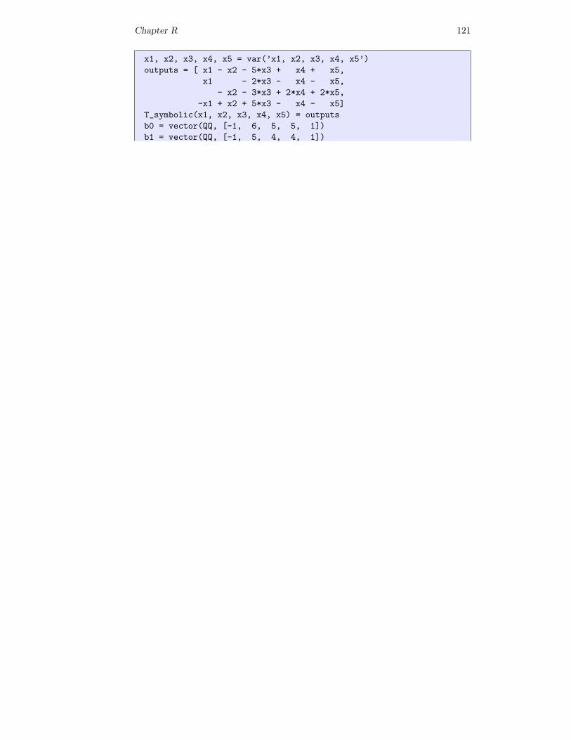
Chapter R 121
x1, x2, x3, x4, x5 = var(’x1, x2, x3, x4, x5’)
outputs = [ x1 - x2 - 5*x3 + x4 + x5,
x1 - 2*x3 - x4 - x5,
- x2 - 3*x3 + 2*x4 + 2*x5,
-x1 + x2 + 5*x3 - x4 - x5]
T_symbolic(x1, x2, x3, x4, x5) = outputs
b0 = vector(QQ, [-1, 6, 5, 5, 1])
b1 = vector(QQ, [-1, 5, 4, 4, 1])
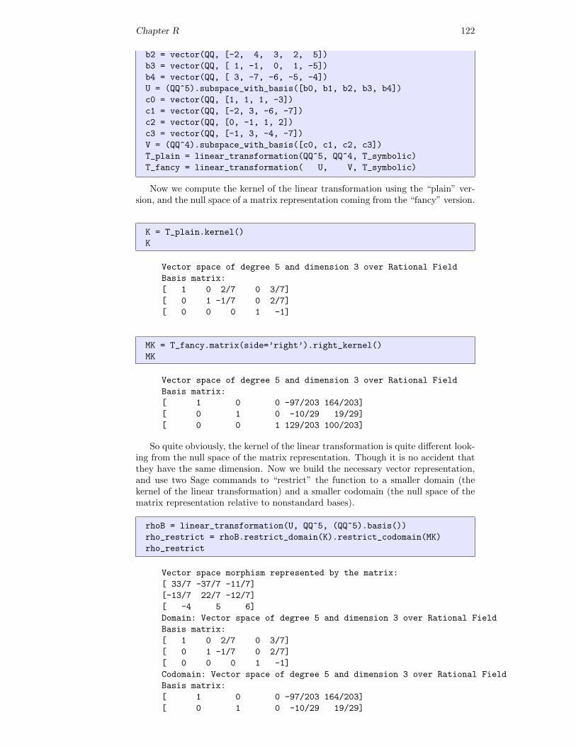
Chapter R 122
b2 = vector(QQ, [-2, 4, 3, 2, 5])
b3 = vector(QQ, [ 1, -1, 0, 1, -5])
b4 = vector(QQ, [ 3, -7, -6, -5, -4])
U = (QQ^5).subspace_with_basis([b0, b1, b2, b3, b4])
c0 = vector(QQ, [1, 1, 1, -3])
c1 = vector(QQ, [-2, 3, -6, -7])
c2 = vector(QQ, [0, -1, 1, 2])
c3 = vector(QQ, [-1, 3, -4, -7])
V = (QQ^4).subspace_with_basis([c0, c1, c2, c3])
T_plain = linear_transformation(QQ^5, QQ^4, T_symbolic)
T_fancy = linear_transformation( U, V, T_symbolic)
Now we compute the kernel of the linear transformation using the “plain” ver-sion, and the null space of a matrix representation coming from the “fancy” version.
K = T_plain.kernel()
K
Vector space of degree 5 and dimension 3 over Rational Field
Basis matrix:
[ 1 0 2/7 0 3/7]
[ 0 1 -1/7 0 2/7]
[ 0 0 0 1 -1]
MK = T_fancy.matrix(side=’right’).right_kernel()
MK
Vector space of degree 5 and dimension 3 over Rational Field
Basis matrix:
[ 1 0 0 -97/203 164/203]
[ 0 1 0 -10/29 19/29]
[ 0 0 1 129/203 100/203]
So quite obviously, the kernel of the linear transformation is quite different look-ing from the null space of the matrix representation. Though it is no accident thatthey have the same dimension. Now we build the necessary vector representation,and use two Sage commands to “restrict” the function to a smaller domain (thekernel of the linear transformation) and a smaller codomain (the null space of thematrix representation relative to nonstandard bases).
rhoB = linear_transformation(U, QQ^5, (QQ^5).basis())
rho_restrict = rhoB.restrict_domain(K).restrict_codomain(MK)
rho_restrict
Vector space morphism represented by the matrix:
[ 33/7 -37/7 -11/7]
[-13/7 22/7 -12/7]
[ -4 5 6]
Domain: Vector space of degree 5 and dimension 3 over Rational Field
Basis matrix:
[ 1 0 2/7 0 3/7]
[ 0 1 -1/7 0 2/7]
[ 0 0 0 1 -1]
Codomain: Vector space of degree 5 and dimension 3 over Rational Field
Basis matrix:
[ 1 0 0 -97/203 164/203]
[ 0 1 0 -10/29 19/29]
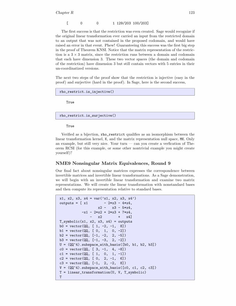
Chapter R 123
[ 0 0 1 129/203 100/203]
The first success is that the restriction was even created. Sage would recognize ifthe original linear transformation ever carried an input from the restricted domainto an output that was not contained in the proposed codomain, and would haveraised an error in that event. Phew! Guaranteeing this success was the first big stepin the proof of Theorem KNSI. Notice that the matrix representation of the restric-tion is a 3 × 3 matrix, since the restriction runs between a domain and codomainthat each have dimension 3. These two vector spaces (the domain and codomainof the restriction) have dimension 3 but still contain vectors with 5 entries in theirun-coordinatized versions.
The next two steps of the proof show that the restriction is injective (easy in theproof) and surjective (hard in the proof). In Sage, here is the second success,
rho_restrict.is_injective()
True
rho_restrict.is_surjective()
True
Verified as a bijection, rho_restrict qualifies as an isomorphism between thelinear transformation kernel, K, and the matrix representation null space, MK. Onlyan example, but still very nice. Your turn — can you create a verfication of The-orem RCSI (for this example, or some other nontrivial example you might createyourself)?
NME9 Nonsingular Matrix Equivalences, Round 9
Our final fact about nonsingular matrices expresses the correspondence betweeninvertible matrices and invertible linear transformations. As a Sage demonstration,we will begin with an invertible linear transformation and examine two matrixrepresentations. We will create the linear transformation with nonstandard basesand then compute its representation relative to standard bases.
x1, x2, x3, x4 = var(’x1, x2, x3, x4’)
outputs = [ x1 - 2*x3 - 4*x4,
x2 - x3 - 5*x4,
-x1 - 2*x2 + 2*x3 + 7*x4,
- x2 + x4]
T_symbolic(x1, x2, x3, x4) = outputs
b0 = vector(QQ, [ 1, -2, -1, 8])
b1 = vector(QQ, [ 0, 1, 0, -2])
b2 = vector(QQ, [-1, -2, 2, -5])
b3 = vector(QQ, [-1, -3, 2, -2])
U = (QQ^4).subspace_with_basis([b0, b1, b2, b3])
c0 = vector(QQ, [ 3, -1, 4, -8])
c1 = vector(QQ, [ 1, 0, 1, -1])
c2 = vector(QQ, [ 0, 2, -1, 6])
c3 = vector(QQ, [-1, 2, -2, 8])
V = (QQ^4).subspace_with_basis([c0, c1, c2, c3])
T = linear_transformation(U, V, T_symbolic)
T
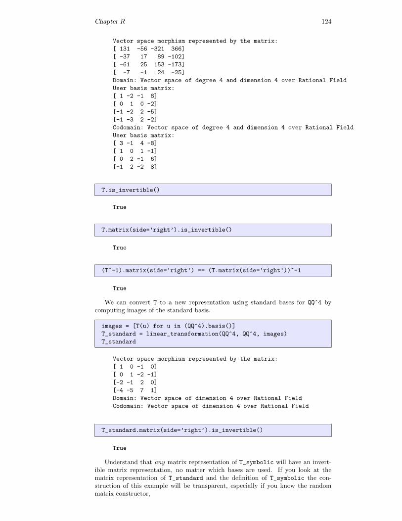
Chapter R 124
Vector space morphism represented by the matrix:
[ 131 -56 -321 366]
[ -37 17 89 -102]
[ -61 25 153 -173]
[ -7 -1 24 -25]
Domain: Vector space of degree 4 and dimension 4 over Rational Field
User basis matrix:
[ 1 -2 -1 8]
[ 0 1 0 -2]
[-1 -2 2 -5]
[-1 -3 2 -2]
Codomain: Vector space of degree 4 and dimension 4 over Rational Field
User basis matrix:
[ 3 -1 4 -8]
[ 1 0 1 -1]
[ 0 2 -1 6]
[-1 2 -2 8]
T.is_invertible()
True
T.matrix(side=’right’).is_invertible()
True
(T^-1).matrix(side=’right’) == (T.matrix(side=’right’))^-1
True
We can convert T to a new representation using standard bases for QQ^4 bycomputing images of the standard basis.
images = [T(u) for u in (QQ^4).basis()]
T_standard = linear_transformation(QQ^4, QQ^4, images)
T_standard
Vector space morphism represented by the matrix:
[ 1 0 -1 0]
[ 0 1 -2 -1]
[-2 -1 2 0]
[-4 -5 7 1]
Domain: Vector space of dimension 4 over Rational Field
Codomain: Vector space of dimension 4 over Rational Field
T_standard.matrix(side=’right’).is_invertible()
True
Understand that any matrix representation of T_symbolic will have an invert-ible matrix representation, no matter which bases are used. If you look at thematrix representation of T_standard and the definition of T_symbolic the con-struction of this example will be transparent, especially if you know the randommatrix constructor,
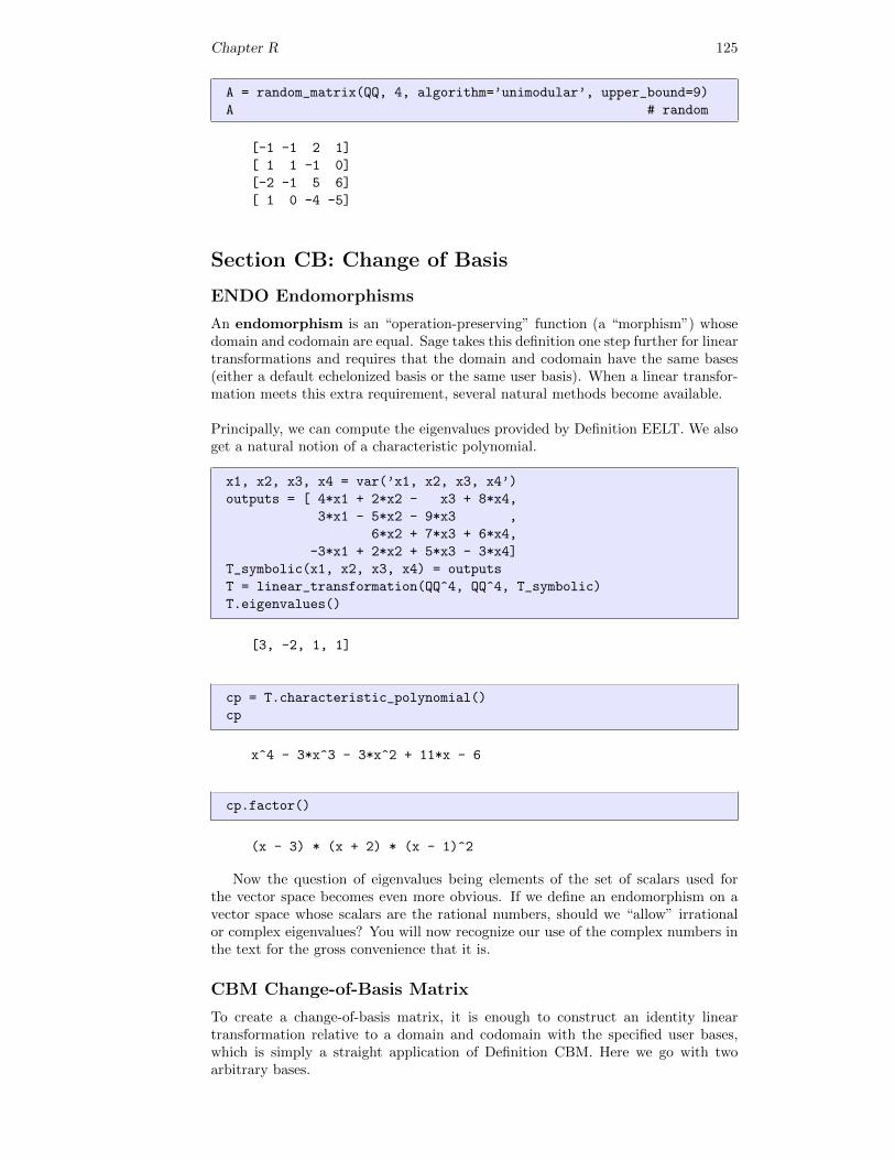
Chapter R 125
A = random_matrix(QQ, 4, algorithm=’unimodular’, upper_bound=9)
A # random
[-1 -1 2 1]
[ 1 1 -1 0]
[-2 -1 5 6]
[ 1 0 -4 -5]
Section CB: Change of Basis
ENDO Endomorphisms
An endomorphism is an “operation-preserving” function (a “morphism”) whosedomain and codomain are equal. Sage takes this definition one step further for lineartransformations and requires that the domain and codomain have the same bases(either a default echelonized basis or the same user basis). When a linear transfor-mation meets this extra requirement, several natural methods become available.
Principally, we can compute the eigenvalues provided by Definition EELT. We alsoget a natural notion of a characteristic polynomial.
x1, x2, x3, x4 = var(’x1, x2, x3, x4’)
outputs = [ 4*x1 + 2*x2 - x3 + 8*x4,
3*x1 - 5*x2 - 9*x3 ,
6*x2 + 7*x3 + 6*x4,
-3*x1 + 2*x2 + 5*x3 - 3*x4]
T_symbolic(x1, x2, x3, x4) = outputs
T = linear_transformation(QQ^4, QQ^4, T_symbolic)
T.eigenvalues()
[3, -2, 1, 1]
cp = T.characteristic_polynomial()
cp
x^4 - 3*x^3 - 3*x^2 + 11*x - 6
cp.factor()
(x - 3) * (x + 2) * (x - 1)^2
Now the question of eigenvalues being elements of the set of scalars used forthe vector space becomes even more obvious. If we define an endomorphism on avector space whose scalars are the rational numbers, should we “allow” irrationalor complex eigenvalues? You will now recognize our use of the complex numbers inthe text for the gross convenience that it is.
CBM Change-of-Basis Matrix
To create a change-of-basis matrix, it is enough to construct an identity lineartransformation relative to a domain and codomain with the specified user bases,which is simply a straight application of Definition CBM. Here we go with twoarbitrary bases.
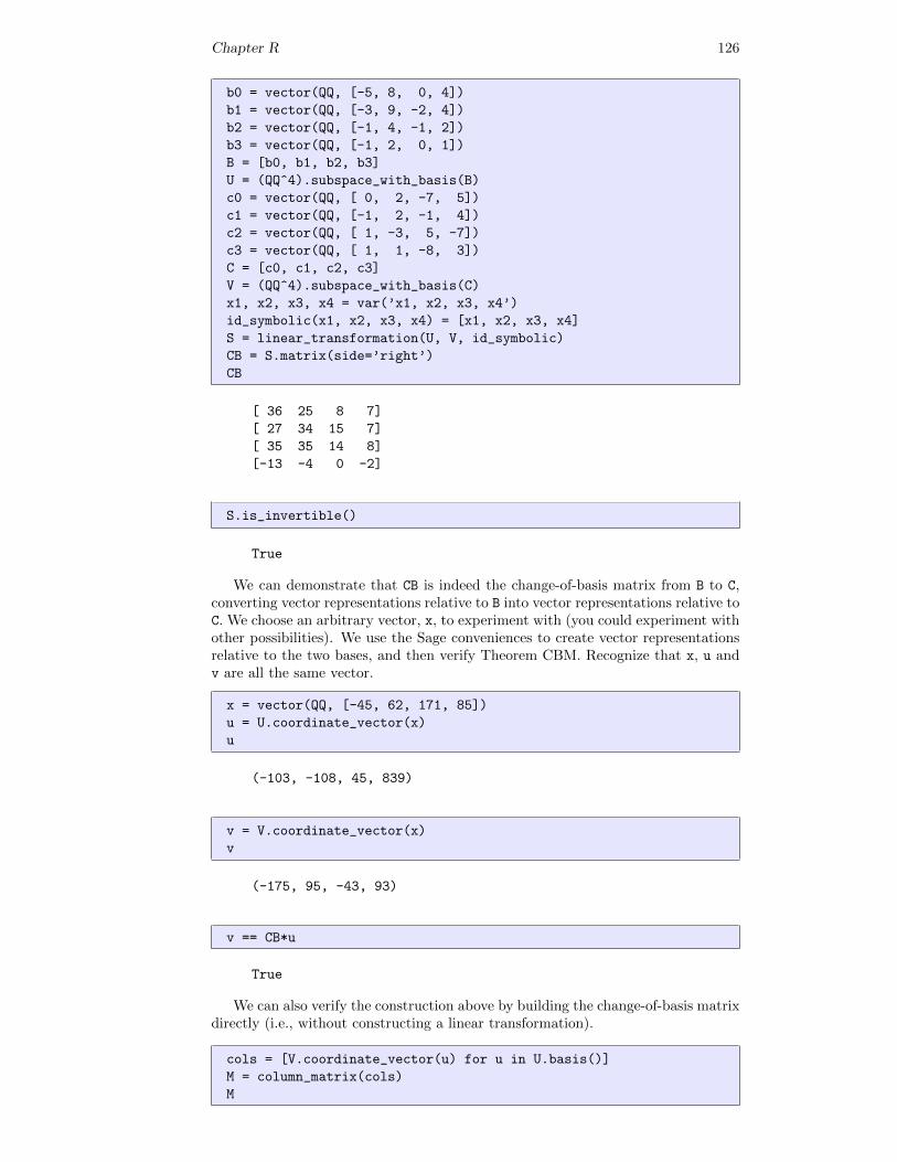
Chapter R 126
b0 = vector(QQ, [-5, 8, 0, 4])
b1 = vector(QQ, [-3, 9, -2, 4])
b2 = vector(QQ, [-1, 4, -1, 2])
b3 = vector(QQ, [-1, 2, 0, 1])
B = [b0, b1, b2, b3]
U = (QQ^4).subspace_with_basis(B)
c0 = vector(QQ, [ 0, 2, -7, 5])
c1 = vector(QQ, [-1, 2, -1, 4])
c2 = vector(QQ, [ 1, -3, 5, -7])
c3 = vector(QQ, [ 1, 1, -8, 3])
C = [c0, c1, c2, c3]
V = (QQ^4).subspace_with_basis(C)
x1, x2, x3, x4 = var(’x1, x2, x3, x4’)
id_symbolic(x1, x2, x3, x4) = [x1, x2, x3, x4]
S = linear_transformation(U, V, id_symbolic)
CB = S.matrix(side=’right’)
CB
[ 36 25 8 7]
[ 27 34 15 7]
[ 35 35 14 8]
[-13 -4 0 -2]
S.is_invertible()
True
We can demonstrate that CB is indeed the change-of-basis matrix from B to C,converting vector representations relative to B into vector representations relative toC. We choose an arbitrary vector, x, to experiment with (you could experiment withother possibilities). We use the Sage conveniences to create vector representationsrelative to the two bases, and then verify Theorem CBM. Recognize that x, u andv are all the same vector.
x = vector(QQ, [-45, 62, 171, 85])
u = U.coordinate_vector(x)
u
(-103, -108, 45, 839)
v = V.coordinate_vector(x)
v
(-175, 95, -43, 93)
v == CB*u
True
We can also verify the construction above by building the change-of-basis matrixdirectly (i.e., without constructing a linear transformation).
cols = [V.coordinate_vector(u) for u in U.basis()]
M = column_matrix(cols)
M
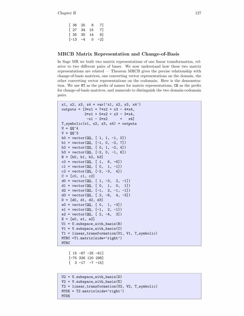
Chapter R 127
[ 36 25 8 7]
[ 27 34 15 7]
[ 35 35 14 8]
[-13 -4 0 -2]
MRCB Matrix Representation and Change-of-Basis
In Sage MR we built two matrix representations of one linear transformation, rel-ative to two different pairs of bases. We now understand how these two matrixrepresentations are related — Theorem MRCB gives the precise relationship withchange-of-basis matrices, one converting vector representations on the domain, theother converting vector representations on the codomain. Here is the demonstra-tion. We use MT as the prefix of names for matrix representations, CB as the prefixfor change-of-basis matrices, and numerals to distinguish the two domain-codomainpairs.
x1, x2, x3, x4 = var(’x1, x2, x3, x4’)
outputs = [3*x1 + 7*x2 + x3 - 4*x4,
2*x1 + 5*x2 + x3 - 3*x4,
-x1 - 2*x2 + x4]
T_symbolic(x1, x2, x3, x4) = outputs
U = QQ^4
V = QQ^3
b0 = vector(QQ, [ 1, 1, -1, 0])
b1 = vector(QQ, [-1, 0, -2, 7])
b2 = vector(QQ, [ 0, 1, -2, 4])
b3 = vector(QQ, [-2, 0, -1, 6])
B = [b0, b1, b2, b3]
c0 = vector(QQ, [ 1, 6, -6])
c1 = vector(QQ, [ 0, 1, -1])
c2 = vector(QQ, [-2, -3, 4])
C = [c0, c1, c2]
d0 = vector(QQ, [ 1, -3, 2, -1])
d1 = vector(QQ, [ 0, 1, 0, 1])
d2 = vector(QQ, [-1, 2, -1, -1])
d3 = vector(QQ, [ 2, -8, 4, -3])
D = [d0, d1, d2, d3]
e0 = vector(QQ, [ 0, 1, -3])
e1 = vector(QQ, [-1, 2, -1])
e2 = vector(QQ, [ 2, -4, 3])
E = [e0, e1, e2]
U1 = U.subspace_with_basis(B)
V1 = V.subspace_with_basis(C)
T1 = linear_transformation(U1, V1, T_symbolic)
MTBC =T1.matrix(side=’right’)
MTBC
[ 15 -67 -25 -61]
[-75 326 120 298]
[ 3 -17 -7 -15]
U2 = U.subspace_with_basis(D)
V2 = V.subspace_with_basis(E)
T2 = linear_transformation(U2, V2, T_symbolic)
MTDE = T2.matrix(side=’right’)
MTDE
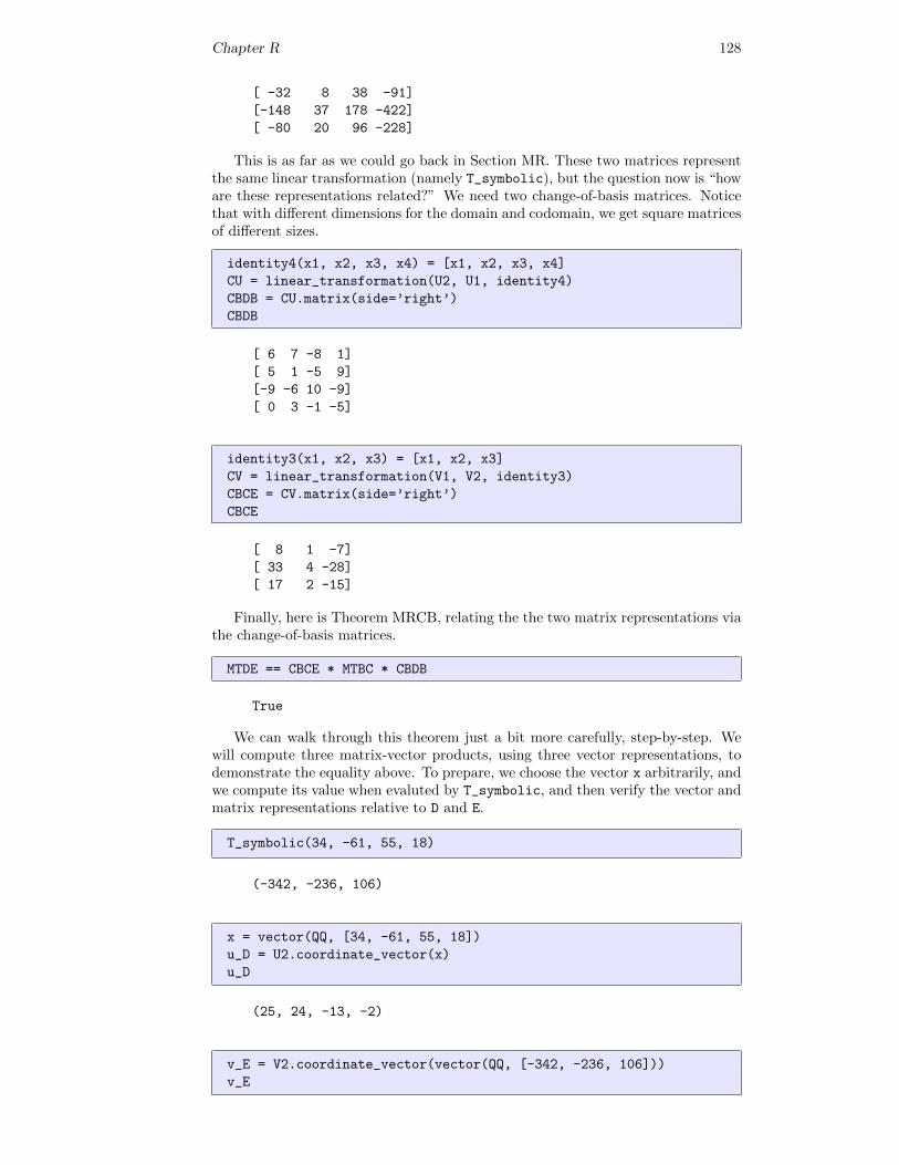
Chapter R 128
[ -32 8 38 -91]
[-148 37 178 -422]
[ -80 20 96 -228]
This is as far as we could go back in Section MR. These two matrices representthe same linear transformation (namely T_symbolic), but the question now is “howare these representations related?” We need two change-of-basis matrices. Noticethat with different dimensions for the domain and codomain, we get square matricesof different sizes.
identity4(x1, x2, x3, x4) = [x1, x2, x3, x4]
CU = linear_transformation(U2, U1, identity4)
CBDB = CU.matrix(side=’right’)
CBDB
[ 6 7 -8 1]
[ 5 1 -5 9]
[-9 -6 10 -9]
[ 0 3 -1 -5]
identity3(x1, x2, x3) = [x1, x2, x3]
CV = linear_transformation(V1, V2, identity3)
CBCE = CV.matrix(side=’right’)
CBCE
[ 8 1 -7]
[ 33 4 -28]
[ 17 2 -15]
Finally, here is Theorem MRCB, relating the the two matrix representations viathe change-of-basis matrices.
MTDE == CBCE * MTBC * CBDB
True
We can walk through this theorem just a bit more carefully, step-by-step. Wewill compute three matrix-vector products, using three vector representations, todemonstrate the equality above. To prepare, we choose the vector x arbitrarily, andwe compute its value when evaluted by T_symbolic, and then verify the vector andmatrix representations relative to D and E.
T_symbolic(34, -61, 55, 18)
(-342, -236, 106)
x = vector(QQ, [34, -61, 55, 18])
u_D = U2.coordinate_vector(x)
u_D
(25, 24, -13, -2)
v_E = V2.coordinate_vector(vector(QQ, [-342, -236, 106]))
v_E
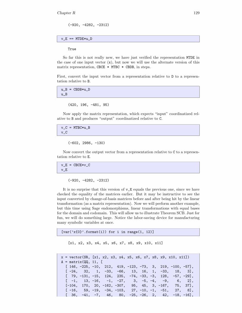
Chapter R 129
(-920, -4282, -2312)
v_E == MTDE*u_D
True
So far this is not really new, we have just verified the representation MTDE inthe case of one input vector (x), but now we will use the alternate version of thismatrix representation, CBCE * MTBC * CBDB, in steps.
First, convert the input vector from a representation relative to D to a represen-tation relative to B.
u_B = CBDB*u_D
u_B
(420, 196, -481, 95)
Now apply the matrix representation, which expects “input” coordinatized rel-ative to B and produces “output” coordinatized relative to C.
v_C = MTBC*u_B
v_C
(-602, 2986, -130)
Now convert the output vector from a representation relative to C to a represen-tation relative to E.
v_E = CBCE*v_C
v_E
(-920, -4282, -2312)
It is no surprise that this version of v_E equals the previous one, since we havechecked the equality of the matrices earlier. But it may be instructive to see theinput converted by change-of-basis matrices before and after being hit by the lineartransformation (as a matrix representation). Now we will perform another example,but this time using Sage endomorphisms, linear transformations with equal basesfor the domain and codomain. This will allow us to illustrate Theorem SCB. Just forfun, we will do something large. Notice the labor-saving device for manufacturingmany symbolic variables at once.
[var(’x{0}’.format(i)) for i in range(1, 12)]
[x1, x2, x3, x4, x5, x6, x7, x8, x9, x10, x11]
x = vector(SR, [x1, x2, x3, x4, x5, x6, x7, x8, x9, x10, x11])
A = matrix(QQ, 11, [
[ 146, -225, -10, 212, 419, -123, -73, 3, 219, -100, -57],
[ -24, 32, 1, -33, -66, 13, 16, 1, -33, 18, 3],
[ 79, -131, -15, 124, 235, -74, -33, -3, 128, -57, -29],
[ -1, 13, -16, -1, -27, 3, -5, -4, -9, 6, 2],
[-104, 170, 20, -162, -307, 95, 45, 3, -167, 75, 37],
[ -16, 59, -19, -34, -103, 27, -10, -1, -51, 27, 8],
[ 36, -41, -7, 46, 80, -25, -26, 2, 42, -18, -16],
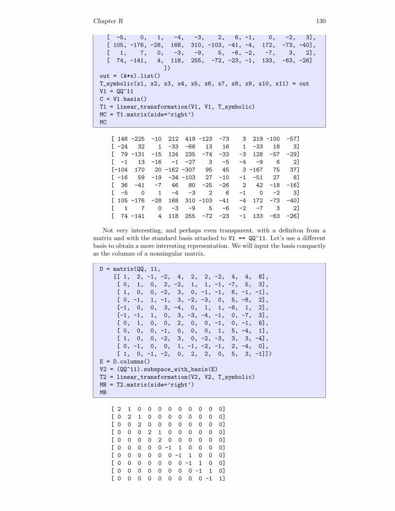
Chapter R 130
[ -5, 0, 1, -4, -3, 2, 6, -1, 0, -2, 3],
[ 105, -176, -28, 168, 310, -103, -41, -4, 172, -73, -40],
[ 1, 7, 0, -3, -9, 5, -6, -2, -7, 3, 2],
[ 74, -141, 4, 118, 255, -72, -23, -1, 133, -63, -26]
])
out = (A*x).list()
T_symbolic(x1, x2, x3, x4, x5, x6, x7, x8, x9, x10, x11) = out
V1 = QQ^11
C = V1.basis()
T1 = linear_transformation(V1, V1, T_symbolic)
MC = T1.matrix(side=’right’)
MC
[ 146 -225 -10 212 419 -123 -73 3 219 -100 -57]
[ -24 32 1 -33 -66 13 16 1 -33 18 3]
[ 79 -131 -15 124 235 -74 -33 -3 128 -57 -29]
[ -1 13 -16 -1 -27 3 -5 -4 -9 6 2]
[-104 170 20 -162 -307 95 45 3 -167 75 37]
[ -16 59 -19 -34 -103 27 -10 -1 -51 27 8]
[ 36 -41 -7 46 80 -25 -26 2 42 -18 -16]
[ -5 0 1 -4 -3 2 6 -1 0 -2 3]
[ 105 -176 -28 168 310 -103 -41 -4 172 -73 -40]
[ 1 7 0 -3 -9 5 -6 -2 -7 3 2]
[ 74 -141 4 118 255 -72 -23 -1 133 -63 -26]
Not very interesting, and perhaps even transparent, with a definiton from amatrix and with the standard basis attached to V1 == QQ^11. Let’s use a differentbasis to obtain a more interesting representation. We will input the basis compactlyas the columns of a nonsingular matrix.
D = matrix(QQ, 11,
[[ 1, 2, -1, -2, 4, 2, 2, -2, 4, 4, 8],
[ 0, 1, 0, 2, -2, 1, 1, -1, -7, 5, 3],
[ 1, 0, 0, -2, 3, 0, -1, -1, 6, -1, -1],
[ 0, -1, 1, -1, 3, -2, -3, 0, 5, -8, 2],
[-1, 0, 0, 3, -4, 0, 1, 1, -8, 1, 2],
[-1, -1, 1, 0, 3, -3, -4, -1, 0, -7, 3],
[ 0, 1, 0, 0, 2, 0, 0, -1, 0, -1, 8],
[ 0, 0, 0, -1, 0, 0, 0, 1, 5, -4, 1],
[ 1, 0, 0, -2, 3, 0, -2, -3, 3, 3, -4],
[ 0, -1, 0, 0, 1, -1, -2, -1, 2, -4, 0],
[ 1, 0, -1, -2, 0, 2, 2, 0, 5, 3, -1]])
E = D.columns()
V2 = (QQ^11).subspace_with_basis(E)
T2 = linear_transformation(V2, V2, T_symbolic)
MB = T2.matrix(side=’right’)
MB
[ 2 1 0 0 0 0 0 0 0 0 0]
[ 0 2 1 0 0 0 0 0 0 0 0]
[ 0 0 2 0 0 0 0 0 0 0 0]
[ 0 0 0 2 1 0 0 0 0 0 0]
[ 0 0 0 0 2 0 0 0 0 0 0]
[ 0 0 0 0 0 -1 1 0 0 0 0]
[ 0 0 0 0 0 0 -1 1 0 0 0]
[ 0 0 0 0 0 0 0 -1 1 0 0]
[ 0 0 0 0 0 0 0 0 -1 1 0]
[ 0 0 0 0 0 0 0 0 0 -1 1]
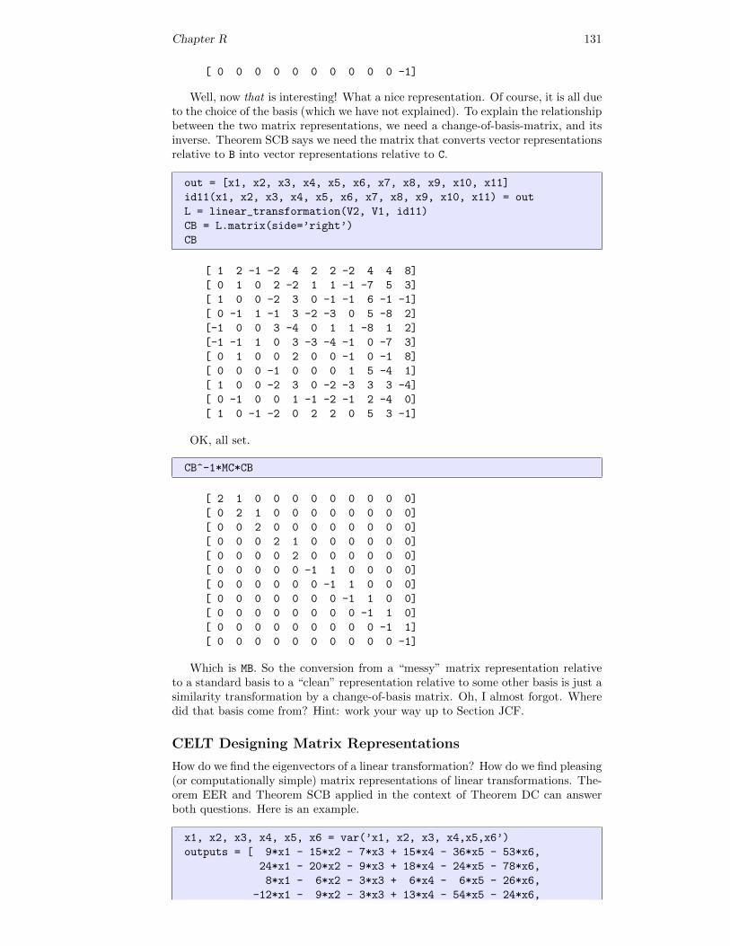
Chapter R 131
[ 0 0 0 0 0 0 0 0 0 0 -1]
Well, now that is interesting! What a nice representation. Of course, it is all dueto the choice of the basis (which we have not explained). To explain the relationshipbetween the two matrix representations, we need a change-of-basis-matrix, and itsinverse. Theorem SCB says we need the matrix that converts vector representationsrelative to B into vector representations relative to C.
out = [x1, x2, x3, x4, x5, x6, x7, x8, x9, x10, x11]
id11(x1, x2, x3, x4, x5, x6, x7, x8, x9, x10, x11) = out
L = linear_transformation(V2, V1, id11)
CB = L.matrix(side=’right’)
CB
[ 1 2 -1 -2 4 2 2 -2 4 4 8]
[ 0 1 0 2 -2 1 1 -1 -7 5 3]
[ 1 0 0 -2 3 0 -1 -1 6 -1 -1]
[ 0 -1 1 -1 3 -2 -3 0 5 -8 2]
[-1 0 0 3 -4 0 1 1 -8 1 2]
[-1 -1 1 0 3 -3 -4 -1 0 -7 3]
[ 0 1 0 0 2 0 0 -1 0 -1 8]
[ 0 0 0 -1 0 0 0 1 5 -4 1]
[ 1 0 0 -2 3 0 -2 -3 3 3 -4]
[ 0 -1 0 0 1 -1 -2 -1 2 -4 0]
[ 1 0 -1 -2 0 2 2 0 5 3 -1]
OK, all set.
CB^-1*MC*CB
[ 2 1 0 0 0 0 0 0 0 0 0]
[ 0 2 1 0 0 0 0 0 0 0 0]
[ 0 0 2 0 0 0 0 0 0 0 0]
[ 0 0 0 2 1 0 0 0 0 0 0]
[ 0 0 0 0 2 0 0 0 0 0 0]
[ 0 0 0 0 0 -1 1 0 0 0 0]
[ 0 0 0 0 0 0 -1 1 0 0 0]
[ 0 0 0 0 0 0 0 -1 1 0 0]
[ 0 0 0 0 0 0 0 0 -1 1 0]
[ 0 0 0 0 0 0 0 0 0 -1 1]
[ 0 0 0 0 0 0 0 0 0 0 -1]
Which is MB. So the conversion from a “messy” matrix representation relativeto a standard basis to a “clean” representation relative to some other basis is just asimilarity transformation by a change-of-basis matrix. Oh, I almost forgot. Wheredid that basis come from? Hint: work your way up to Section JCF.
CELT Designing Matrix Representations
How do we find the eigenvectors of a linear transformation? How do we find pleasing(or computationally simple) matrix representations of linear transformations. The-orem EER and Theorem SCB applied in the context of Theorem DC can answerboth questions. Here is an example.
x1, x2, x3, x4, x5, x6 = var(’x1, x2, x3, x4,x5,x6’)
outputs = [ 9*x1 - 15*x2 - 7*x3 + 15*x4 - 36*x5 - 53*x6,
24*x1 - 20*x2 - 9*x3 + 18*x4 - 24*x5 - 78*x6,
8*x1 - 6*x2 - 3*x3 + 6*x4 - 6*x5 - 26*x6,
-12*x1 - 9*x2 - 3*x3 + 13*x4 - 54*x5 - 24*x6,
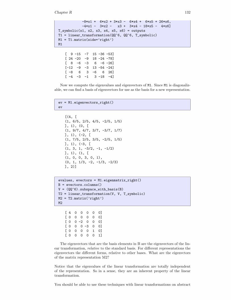
Chapter R 132
-8*x1 + 6*x2 + 3*x3 - 6*x4 + 6*x5 + 26*x6,
-4*x1 - 3*x2 - x3 + 3*x4 - 18*x5 - 4*x6]
T_symbolic(x1, x2, x3, x4, x5, x6) = outputs
T1 = linear_transformation(QQ^6, QQ^6, T_symbolic)
M1 = T1.matrix(side=’right’)
M1
[ 9 -15 -7 15 -36 -53]
[ 24 -20 -9 18 -24 -78]
[ 8 -6 -3 6 -6 -26]
[-12 -9 -3 13 -54 -24]
[ -8 6 3 -6 6 26]
[ -4 -3 -1 3 -18 -4]
Now we compute the eigenvalues and eigenvectors of M1. Since M1 is diagonaliz-able, we can find a basis of eigenvectors for use as the basis for a new representation.
ev = M1.eigenvectors_right()
ev
[(4, [
(1, 6/5, 2/5, 4/5, -2/5, 1/5)
], 1), (0, [
(1, 9/7, 4/7, 3/7, -3/7, 1/7)
], 1), (-2, [
(1, 7/5, 2/5, 3/5, -2/5, 1/5)
], 1), (-3, [
(1, 3, 1, -3/2, -1, -1/2)
], 1), (1, [
(1, 0, 0, 3, 0, 1),
(0, 1, 1/3, -2, -1/3, -2/3)
], 2)]
evalues, evectors = M1.eigenmatrix_right()
B = evectors.columns()
V = (QQ^6).subspace_with_basis(B)
T2 = linear_transformation(V, V, T_symbolic)
M2 = T2.matrix(’right’)
M2
[ 4 0 0 0 0 0]
[ 0 0 0 0 0 0]
[ 0 0 -2 0 0 0]
[ 0 0 0 -3 0 0]
[ 0 0 0 0 1 0]
[ 0 0 0 0 0 1]
The eigenvectors that are the basis elements in B are the eigenvectors of the lin-ear transformation, relative to the standard basis. For different representations theeigenvectors tke different forms, relative to other bases. What are the eigenvctorsof the matrix representation M2?
Notice that the eigenvalues of the linear transformation are totally independentof the representation. So in a sense, they are an inherent property of the lineartransformation.
You should be able to use these techniques with linear transformations on abstract
Chapter R 133
vector spaces — just use a mental linear transformation transforming the abstractvector space back-and-forth between a vector space of column vectors of the rightsize.
SUTH4 Sage Under The Hood, Round 4
We finally have enough theorems to understand how Sage creates and manageslinear transformations. With a choice of bases for the domain and codomain, alinear transformation can be represented by a matrix. Every interesting property ofthe linear transformation can be computed from the matrix representation, and wecan convert between representations (of vectors and linear transformations) withchange-of-basis matrices, similarity and matrix multiplication.
So we can understand the theory of linear algebra better by experimenting withthe assistance of Sage, and the theory of linear algebra helps us understand howSage is designed and functions. A virtuous cycle, if there ever was one. Keep itgoing.