Sage: Open Source Mathematics Software

Korean Mathematics SocietySpring Meeting

Prof. Robert BeezerUniversity of Puget Sound

Tacoma, Washington USA

April 28, 2012

What is Sage?

• An open source system for advanced mathematics.

• An open source mathematics distribution (like Linux) with Python asthe glue.

• A tool for mathematics research.

• A tool for teaching mathematics.

Mission Statement

1

Create a viable free open source alternative to Magma,Maple, Mathematica, and Matlab.

An overview:

• Created in 2005 by William Stein.

• GPL license.

• Includes about 100 open source packages.

• Now has around 500,000 lines of new code,by several hundred mathematician-programmers.

The Sage Notebook

A symbolic derivative (from Maxima).

f(x) = x^3*e^-x

df = f.derivative()

df

Derivative of a function is again a function, and can be evaluated.

slope = df(4)

slope

Arbitrary precision numerical values on request (from MPmath).

N(slope, digits=20)

Can display plots in the notebook (matplotlib).

plot(df, 0, 10, color=’red’, thickness=5)

Interactive demonstrations are easy to create with the “interact” decora-tor and modified function arguments.

2

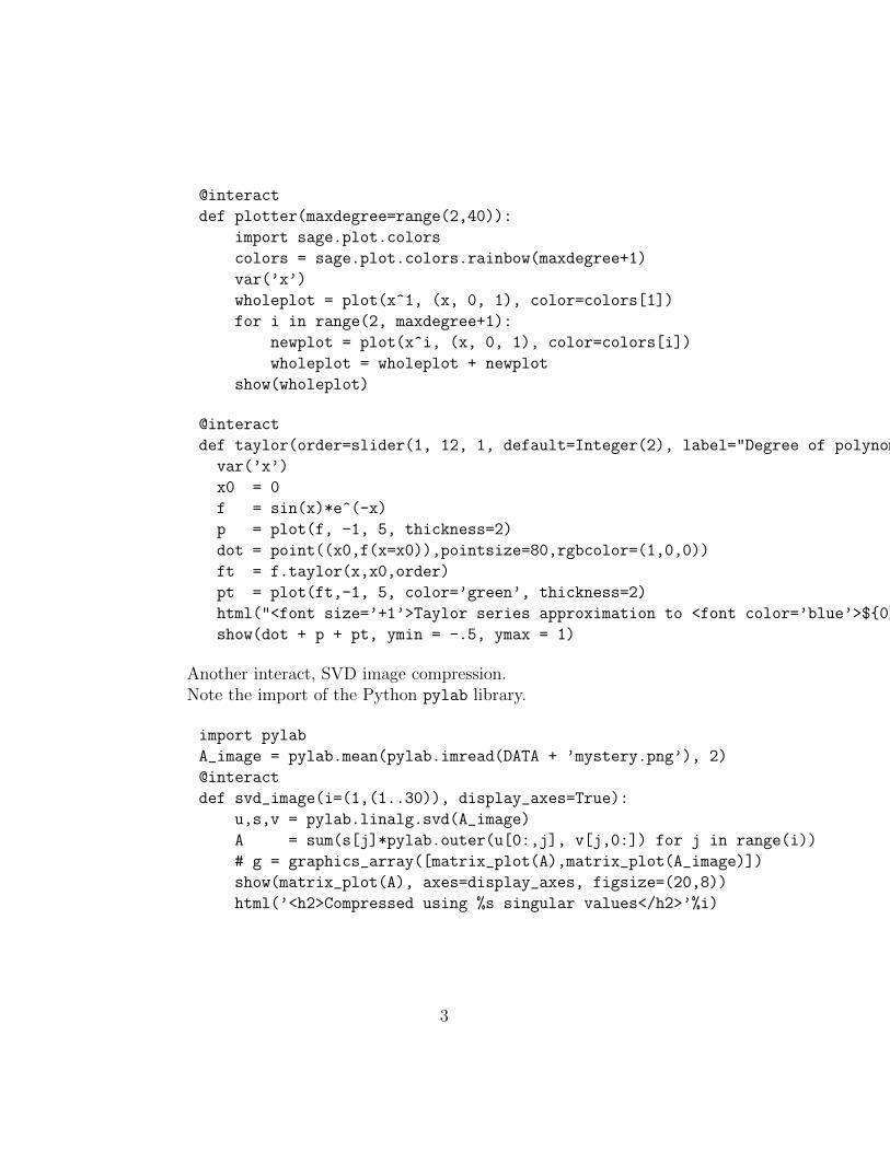
@interact

def plotter(maxdegree=range(2,40)):

import sage.plot.colors

colors = sage.plot.colors.rainbow(maxdegree+1)

var(’x’)

wholeplot = plot(x^1, (x, 0, 1), color=colors[1])

for i in range(2, maxdegree+1):

newplot = plot(x^i, (x, 0, 1), color=colors[i])

wholeplot = wholeplot + newplot

show(wholeplot)

@interact

def taylor(order=slider(1, 12, 1, default=Integer(2), label="Degree of polynomial $\hat{f}$")):

var(’x’)

x0 = 0

f = sin(x)*e^(-x)

p = plot(f, -1, 5, thickness=2)

dot = point((x0,f(x=x0)),pointsize=80,rgbcolor=(1,0,0))

ft = f.taylor(x,x0,order)

pt = plot(ft,-1, 5, color=’green’, thickness=2)

html("<font size=’+1’>Taylor series approximation to <font color=’blue’>${0}$</font> of degree {1} at <font color=’red’>$x={2}$</font></font>".format(latex(f), Integer(order), x0) )

show(dot + p + pt, ymin = -.5, ymax = 1)

Another interact, SVD image compression.Note the import of the Python pylab library.

import pylab

A_image = pylab.mean(pylab.imread(DATA + ’mystery.png’), 2)

@interact

def svd_image(i=(1,(1..30)), display_axes=True):

u,s,v = pylab.linalg.svd(A_image)

A = sum(s[j]*pylab.outer(u[0:,j], v[j,0:]) for j in range(i))

# g = graphics_array([matrix_plot(A),matrix_plot(A_image)])

show(matrix_plot(A), axes=display_axes, figsize=(20,8))

html(’<h2>Compressed using %s singular values</h2>’%i)

3

LaTeX Integration

. . . is superb.

A = random_matrix(QQ, 10, 10)

A

latex(A)

With ”typeset” button checked.

A = random_matrix(QQ, 10, 10)

A

Documentation

A huge number of examples are provided for (a) learning to use Sage com-mands, and (b) to test Sage commands. We call these “doctests.”

M = matrix(QQ, [[1, -2, 2], [-4, 5, 6], [1, 2, 4]])

M

Illustrate tab-completion (rational form), help (doctests), source code

M.

Multivariate Calculus

Study the integral

∫ 4

−4

∫ x2

0

y2 − 10x2 dy dx.

We can add text to our notebooks using TeX syntax and dollar signs.\int_0^4\int_0^{x^2} y^2-10x^2\,dy\,dx

4

var(’x y z’)

integral(integral(y^2-10*x^2, (y, 0, x^2)), (x, -4, 4))

surface = plot3d(y^2-10*x^2, (x, -4, 4), (y, 0, 16))

show(surface)

region = implicit_plot3d(y-x^2, (x, -4, 4), (y, 0, 16), (z, 0, 98), color=’red’, opacity=0.20)

show(surface+region)

A 3-D interact.

# 3-D motion and vector calculus

# Copyright 2009, Robert A. Beezer

# Creative Commons BY-SA 3.0 US

#

#

# 2009/02/15 Built on Sage 3.3.rc0

# 2009/02/17 Improvements from Jason Grout

#

# variable parameter is t

# later at a particular value named t0

#

# un-comment double hash (##) to get

# time-consuming torsion computation

#

var(’t’)

#

# parameter range

#

start=-4*pi

stop=8*pi

#

# position vector definition

# edit here for new example

# example is wide ellipse

# adjust figsize in final show() to get accurate aspect ratio

#

5

a=1/(8*pi)

c=(3/2)*a

position=vector( (exp(a*t)*cos(t), exp(a*t)*sin(t), exp(c*t)) )

#

# graphic of the motion itself

#

path = parametric_plot3d( position(t).list(), (t, start, stop), color = "black" )

#

# derivatives of motion, lengths, unit vectors, etc

#

velocity = derivative( position, t)

acceleration = derivative(velocity, t)

speed = velocity.norm()

speed_deriv = derivative(speed, t)

tangent = (1/speed)*velocity

dT = derivative(tangent, t)

normal = (1/dT.norm())*dT

binormal = tangent.cross_product(normal)

## dB = derivative(binormal, t)

#

# interact section

# slider for parameter, 24 settings

# checkboxes for various vector displays

# computations at one value of parameter, t0

#

@interact

def _(t0 = slider(float(start), float(stop), float((stop-start)/24), float(start) , label = "Parameter"),

pos_check = ("Position", True),

vel_check = ("Velocity", False),

tan_check = ("Unit Tangent", True),

nor_check = ("Unit Normal", True),

bin_check = ("Unit Binormal", True),

acc_check = ("Acceleration", False),

tancomp_check = ("Tangential Component", False),

norcomp_check = ("Normal Component", False)

):

#

# location of interest

6

#

pos_tzero = position(t0)

#

# various scalar quantities at point

#

speed_component = speed(t0)

tangent_component = speed_deriv(t0)

normal_component = sqrt( acceleration(t0).norm()^2 - tangent_component^2 )

curvature = normal_component/speed_component^2

## torsion = (1/speed_component)*(dB(t0)).dot_product(normal(t0))

#

# various vectors, mostly as arrows from the point

#

pos = arrow3d((0,0,0), pos_tzero, rgbcolor=(0,0,0))

tan = arrow3d(pos_tzero, pos_tzero + tangent(t0), rgbcolor=(0,1,0) )

vel = arrow3d(pos_tzero, pos_tzero + velocity(t0), rgbcolor=(0,0.5,0))

nor = arrow3d(pos_tzero, pos_tzero + normal(t0), rgbcolor=(0.5,0,0))

bin = arrow3d(pos_tzero, pos_tzero + binormal(t0), rgbcolor=(0,0,0.5))

acc = arrow3d(pos_tzero, pos_tzero + acceleration(t0), rgbcolor=(1,0,1))

tancomp = arrow3d(pos_tzero, pos_tzero + tangent_component*tangent(t0), rgbcolor=(1,0,1) )

norcomp = arrow3d(pos_tzero, pos_tzero + normal_component*normal(t0), rgbcolor=(1,0,1))

#

# accumulate the graphic based on checkboxes

#

picture = path

if pos_check:

picture = picture + pos

if vel_check:

picture = picture + vel

if tan_check:

picture = picture+ tan

if nor_check:

picture = picture + nor

if bin_check:

picture = picture + bin

if acc_check:

picture = picture + acc

if tancomp_check:

7

picture = picture + tancomp

if norcomp_check:

picture = picture + norcomp

#

# print textual info

#

print "Position vector: r(t)=", position(t)

print "Speed is ", N(speed(t0))

print "Curvature is ", N(curvature)

## print "Torsion is ", N(torsion)

print

print "Right-click on graphic to zoom to 400%"

print "Drag graphic to rotate"

#

# show accumulated graphical info

#

show(picture, aspect_ratio=[1,1,1])

Mature, Reliable Foundation

Gap console, r object, scipy, IMLSage is built on a solid foundation of open source packages for specific

areas of mathematics.

• Groups, Algorithms, Programming (GAP) - group theory

• PARI - rings, finite fields, field extensions

• Singular - commutative algebra

• SciPy/NumPy - scientific computing, numerical linear algebra

• Integer Matrix Library (IML) - integer, rational matrices

• CVXOPT - linear programming, optimization

• NetworkX - graph theory

8

• Pynac - symbolic manipulation

• Maxima - calculus, differential equations

Group Theory

An example: permutation groups are built on GAP.

G = DihedralGroup(8)

G

G.list()

G.is_abelian()

sg = G.subgroups()

[H.order() for H in sg]

H = sg[14]

H.list()

H.is_normal(G)

Exact Linear Algebra

Exact linear algebra over integers and rationals powered by Integer MatrixLibrary (IML).

A = matrix(QQ,

[[1, -2, 3, 2, -1, -4, -3, 4],

[3, -2, 2, 5, 0, 6, -5, -5],

[0, -1, 2, 1, -2, -4, -1, 4],

[-3, 2, -1, -1, -6, -3, 5, 3],

[3, -4, 4, 0, 7, -7, -7, 6]])

A

A.rref()

b = vector(QQ, [2, -1, 3, 4, -3])

A.solve_right(b)

A matrix kernel (null space) is a vector space.

A.right_kernel(basis=’pivot’)

9

Numerical Linear Algebra

Numerical linear algebra is supplied by SciPy, through to LAPACK, ATLAS,BLAS.

A matrix of double-floating point real numbers (RDF).

B = matrix(RDF,

[[0.4706, 0.3436, 0.7156, 0.1706, 0.3863, 0.222, -0.9673],

[0.9433, -0.7333, -0.2906, -0.5203, 0.3548, 0.7577, 0.3936],

[-0.8998, 0.9269, -0.9646, -0.2294, -0.8171, 0.4568, 0.5949],

[0.8814, 0.89, -0.2059, 0.7434, -0.1642, 0.6918, 0.7113],

[-0.0034, -0.9842, 0.7213, -0.7196, -0.7422, 0.3335, 0.5829],

[-0.5676, 0.6433, -0.2296, 0.2681, 0.2992, 0.6988, 0.3332],

[0.0366, -0.5788, 0.5882, 0.1559, -0.6434, 0.871, -0.6518]])

B

Q, R = B.QR()

Q

(Q.conjugate_transpose()*Q).round(4)

R.round(4)

(Q*R-B).round(4)

Honest

Sage is built by teachers, for teachers (and researchers). The curriculumdrives development, not the other way around. And the tool grows withstudents.

Linear Algebra

Linear algebra: vector spaces act like vector spaces.Theorem: N(B) ⊆ N(AB).

10

A = random_matrix(QQ, 3, 4, num_bound = -9, den_bound = 9)

B = random_matrix(QQ, 4, 6, num_bound = -9, den_bound = 9)

NB = B.right_kernel()

NAB = (A*B).right_kernel()

print A

print

print B

print

NB.is_subspace(NAB)

Linear algebra: eigenvalues are algebraic numbers.

A = matrix(QQ, [[2, 2], [-1, 1]])

A

A.characteristic_polynomial()

ev = A.eigenvalues()

ev

rho = ev[0]

rho.parent()

Evaluate in characteristic polynomial.

evaluation = rho^2-3*rho+4

evaluation

evaluation == 0

Algebraic numbers are backed by number fields.

rho.as_number_field_element()

11

Graph Theory

Sage “knows” many interesting graphs.

graphs.

3-element subsets of a 7-set. Edge joins if sets are disjoint.

O4 = graphs.OddGraph(4)

O4.plot()

O4.diameter()

O4.chromatic_number()

O3 is the Petersen graph.

O3 = graphs.OddGraph(3)

P = graphs.PetersenGraph()

graphs_list.show_graphs([O3, P])

Not obvious it is. But we have graph isomorphism handy.

P.is_isomorphic(O3)

Powerful

Sage has realistic mathematical objects.

Finite Fields

F.<a> = FiniteField(3^4)

F

F.polynomial()

a^4

12

F.list()

powers = [a^i for i in [0..79]]

powers

sorted(powers + [F(0)]) == sorted(F.list())

y = 2*a^3 + 2*a^2 + a + 2

y.log(a)

y.log(a^4)

Coercion

How does Sage (or you?) know how to handle 5 + 43?

(Coercion – automatic conversion between number systems.)A finite field is a vector space over its prime subfield.

V = F.vector_space()

V.list()

Can coerce field elements into the vector space, or vice versa.

x = a^34

x

v = V(x)

v

F(v)

Cython

A Sage-inspired project to convert Python to C, then compile.Factorial, Python-style.

def py_fact(n):

fact = 1

for i in range(n):

fact = fact*(i+1)

return fact

13

py_fact(12)

timeit(’py_fact(12)’)

Cython-style.(Iteration 2: cdef, long in header)

%cython

def cy_fact(n):

cdef:

long fact, i

fact = 1

for i in range(n):

fact = fact*(i+1)

return fact

cy_fact(12)

timeit(’cy_fact(12)’)

Speed

Linear algebra is fast, number theory is fast. Arbitrary-precision real num-bers, polynomials are fast. Probably lots of other things I don’t know aboutare also fast.

A = random_matrix(ZZ, 200, 200)

A[100:105, 100:105]

A.determinant()

timeit("A.determinant()")

timeit("A.echelon_form()")

timeit("A.characteristic_polynomial()")

14

Versatile

• Command-line version.

• Notebook with local server.

• Notebook with remote server.

• Sage single cell server.

Demonstration: Open Textbooks with Sage

Tom Judson’s “Abstract Algebra” with Sage exercises.(http://abstract.ups.edu)

RAB’s “A First Course in Linear Algebra” with knowls and Sage cells.(http://linear.ups.edu)

American Institute of Mathhttp://aimath.org/textbooks/beezer/

Personal experimenthttp://beezers.org/sb040-knowl-single/EEsection.html

Home Page exampleshttp://buzzard.ups.edu/home.html

This worksheet available at:http://buzzard.ups.edu/talks.html

15

16