SAGD Operations in the Presence of Overlying Gas Cap … discussion above ignored the effect of thief zones. In the presence of thief zones, especially depleted ones, there is concern

June 2002, Volume 41, No. 6 1

IntroductionMany bituminous reservoirs in Alberta contain overlying gas.

The gas owners would like to produce the gas. However, there isconcern as to whether or not gas production might adverselyaffect any possible bitumen recovery process in the future. Theprimary candidate recovery method for such bitumen formationsis the Steam-Assisted Gravity Drainage (SAGD)(1) process. Theobjective of this study is to examine the feasibility of bitumenrecovery from the underlying sands, and to determine the effect of

“prior” gas production on the process.The effects of overlying gas and/or water sands on the SAGD

process are presented first. This is followed by a discussion of theeffect of continuous and discontinuous shale layers, and theirincorporation in the numerical model, along with the determina-tion of rock properties. Thermal simulation results and conclu-sions follow.

BackgroundThe UTF project demonstrated the viability of the SAGD

process for production of some of the bituminous reservoirs ofAlberta(2, 3), where more conventional thermal processes are lesssuccessful due to immobility of the bitumen at reservoir condi-tions. At the UTF site, the bitumen is capped with a competentshale layer, which confines the vertical expansion of the steamchamber. In many other areas, however, the bitumen is overlainby water and/or gas layers, which can act as “thief zones.”Simulation studies have been conducted(4, 5) and commercialSAGD pilot projects(6, 7) are underway to examine the feasibilityof bitumen recovery, in the presence of these top gas and/or waterlayers. A point of particular concern is whether a low pressure inthe upper zones is detrimental to bitumen recovery. In the nextsection, the interaction between the steam chamber and the uppersands, and the effect of steam-chamber pressure on bitumenrecovery are discussed.

Effect of Steam-Chamber Pressure on theSAGD Process

Steam in the steam chamber is at saturated conditions.Therefore, the steam temperature is determined by its pressure. Ahigher steam pressure leads to higher temperature and lower oilviscosity. This in turn, leads to a higher oil flow rate. On the otherhand, higher steam pressure leads to lower thermal efficiency andhigher Steam-Oil Ratio (SOR). Some of the reasons for largerSOR are that steam at higher pressures has less latent heat, moreheat will leave the reservoir through the produced fluids at highertemperature, and more heat will be left in the steam chamberwhere oil is no longer present(8). To determine the optimum steampressure leading to the best economic performance, sensitivitystudies need to be performed(9).

The pressure in the steam chamber also has a large effect on thechoice of the production system. A higher pressure would allownatural lift of the produced fluids. When pressure is reduced, arti-ficial lift becomes necessary. High-temperature pumping systemsare being developed for operation at low bottomhole pressures(6).

SAGD Operations in the Presence of Overlying Gas Cap and Water Layer—Effect of Shale Layers

M. POOLADI-DARVISHUniversity of Calgary

L. MATTARFekete Associates Inc.

AbstractThe technical and commercial success of SAGD projects over

the past decade has opened the door to the development of alarge number of bitumen reservoirs in Canada, previouslythought uneconomical to produce. Some of these reservoirs haveoverlying gas caps and/or water zones. Some studies have sug-gested that gas-cap production might “sterilize” the underlyingbitumen. Many such studies however, assumed rather thick con-tinuous pays with high permeability, and considered an infinitegas-cap.

In this work, a simulation study was conducted to examinethe feasibility of bitumen production from a certain project areain Alberta, using the SAGD process, and to study the effect ofproduction from the gas cap. A decision needed to be made as towhether gas production should be delayed until after bitumenproduction. The large well spacing did not allow a detaileddescription of the connectivity of the shale layers. The uncer-tainty was compounded by the geological setting of the studyarea, a system of channel sands cut through the original marinesand and shale deposits. Since the actual shale connectivity andthickness was unknown, a methodology was developed to incor-porate different geological descriptions using the available coreand log data. Five reservoir models were developed. Bitumenrecovery, average oil production rate, and cumulative steam-oilratio (SOR) obtained from thermal simulation were the threemain parameters used for evaluation of the attractiveness ofbitumen recovery operations. These numbers were comparedwith some of the corresponding values reported and/or forecastfor economically feasible operations such as the UTF andChristina Lake projects. The effect of pressure reduction (causedby gas-cap production) on production rate and SOR was alsoinvestigated.

The results indicated that for conditions considered in thisstudy the effect of gas production on bitumen recovery wasminor, and appeared as a small deceleration of the recovery anda small increase in SOR.

PAPER: 2001-178

PEER REVIEWED PAPER (“REVIEW AND PUBLICATION PROCESS” CAN BE FOUND ON OUR WEB SITE)

The discussion above ignored the effect of thief zones. In thepresence of thief zones, especially depleted ones, there is concernabout SAGD performance; flow of steam into the thief zone couldlead to excessive steam loss. In such a situation, detailed engineer-ing studies, including numerical simulation are needed to provideanswers to many questions such as:

1. Is there direct communication between the lower sand andthe upper water/gas sands?

2. What are the important performance parameters such asSOR, oil production rate and recovery at the original gas-cappressure?

3. What is the effect of the gas/water cap pressure on these per-formance parameters?

4. Can the steam chamber pressure be balanced with the gas-cap pressure to avoid steam loss? In the case of a top-watersand, can the balanced pressure prevent the top-water fromflowing into the steam chamber?

In this work, we provide the answers to the two middle ques-tions in relation to the bitumen reserves in a particular project areain Alberta.

Geological ConsiderationsMuch of the bituminous reservoirs of the McMurray formation

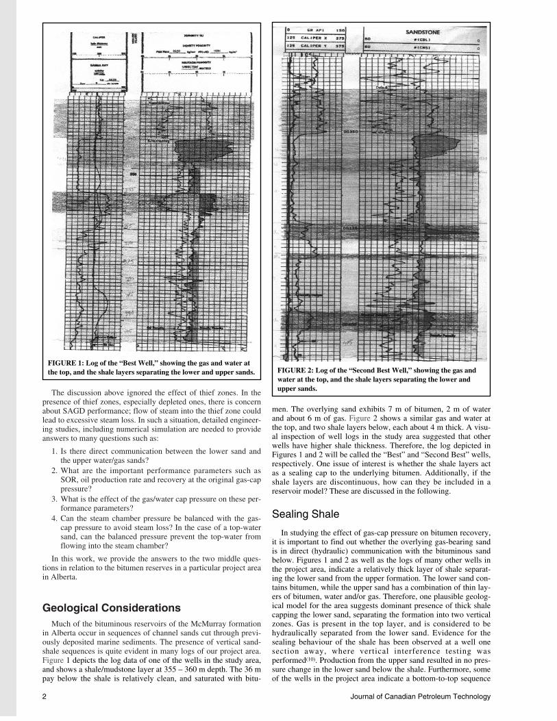
in Alberta occur in sequences of channel sands cut through previ-ously deposited marine sediments. The presence of vertical sand-shale sequences is quite evident in many logs of our project area.Figure 1 depicts the log data of one of the wells in the study area,and shows a shale/mudstone layer at 355 – 360 m depth. The 36 mpay below the shale is relatively clean, and saturated with bitu-

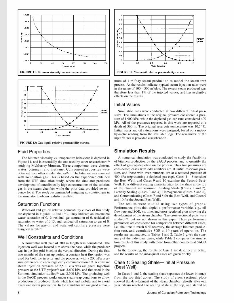
men. The overlying sand exhibits 7 m of bitumen, 2 m of waterand about 6 m of gas. Figure 2 shows a similar gas and water atthe top, and two shale layers below, each about 4 m thick. A visu-al inspection of well logs in the study area suggested that otherwells have higher shale thickness. Therefore, the log depicted inFigures 1 and 2 will be called the “Best” and “Second Best” wells,respectively. One issue of interest is whether the shale layers actas a sealing cap to the underlying bitumen. Additionally, if theshale layers are discontinuous, how can they be included in areservoir model? These are discussed in the following.

Sealing Shale

In studying the effect of gas-cap pressure on bitumen recovery,it is important to find out whether the overlying gas-bearing sandis in direct (hydraulic) communication with the bituminous sandbelow. Figures 1 and 2 as well as the logs of many other wells inthe project area, indicate a relatively thick layer of shale separat-ing the lower sand from the upper formation. The lower sand con-tains bitumen, while the upper sand has a combination of thin lay-ers of bitumen, water and/or gas. Therefore, one plausible geolog-ical model for the area suggests dominant presence of thick shalecapping the lower sand, separating the formation into two verticalzones. Gas is present in the top layer, and is considered to behydraulically separated from the lower sand. Evidence for thesealing behaviour of the shale has been observed at a well onesection away, where vertical interference testing wasperformed(10). Production from the upper sand resulted in no pres-sure change in the lower sand below the shale. Furthermore, someof the wells in the project area indicate a bottom-to-top sequence

2 Journal of Canadian Petroleum Technology

FIGURE 1: Log of the “Best Well,” showing the gas and water atthe top, and the shale layers separating the lower and upper sands. FIGURE 2: Log of the “Second Best Well,” showing the gas and

water at the top, and the shale layers separating the lower andupper sands.

of bitumen, gas, shale, bitumen, and then gas(10). The presence ofgas below the shale would suggest that the shale could act as aseal to a future steam-chamber below.

One might propose, however, that shale layers could be discon-tinuous and gas production from the upper sand would lead toreduced pressure in the formation below. This also, would be ofno harm to the process so long as there is no thief zone rightabove the well pattern, and the overlying shale confines the steamchamber. This is because the SAGD operating pressure is inde-pendent of the initial pressure. SAGD operation in such a reser-voir could be initiated, ignoring the effect of the gas cap at thetop. When the steam chamber approaches the sealing shale, itexpands sideways and develops a normal SAGD steam chamber.The geological model, where the shale barrier is continuous overthe lateral domain of a SAGD well-pair, is the first geological rep-resentation in our simulation study, and is called the Sealing-Shale model.

Discontinuous ShaleAnother probable geological model is that the thick shale at the

top of the lower bitumen is not sealing to the rise of the steamchamber. Under this situation, the way the shale is represented inthe simulation model has a large impact on the results. In hetero-geneous formations, such as that present at the location of interest,it would be impractical to obtain exact geological information ofthe sand and shale sequences. Simple approaches, such as assum-ing a homogeneous formation by ignoring the shales, and the so-called chimney(7) model have been previously used. In this paper,we investigate a methodology to incorporate the effect of theshales objectively.

Implementing an averaging technique to take into account theheterogeneity of the formation, and a stochastic representationbased on geostatistical methods along with multiple simulationruns are two feasible approaches. To construct a geostatisticalreservoir model, log and core data are used to predict the continu-ity of shale and sand layers. Special techniques are then used todistribute shale/sand sequences throughout the area of interest.These techniques generate a prohibitively large number of reser-voir models, all honouring the available data, and therefore allbeing equally probable. In order to avoid numerical simulation ofall the realisations, a few of the reservoir models are chosen.Conventionally, cases are chosen that are believed to lead to best,worst and intermediate recovery to generate a range of equallyprobable recoveries(11). At the UTF, the pilot project area wasdensely drilled – every 100 m along the length of the well, andevery 35 m perpendicular to the well. There, a stochastic represen-tation of shale layers was generated and 30 simulation modelswere built for numerical simulation of the SAGD process(3). Asampling density such as the UTF pilot is often impractical. In ournumerical modelling, we used an alternative averaging techniqueto account for the effect of the shale layers.

Modelling the Shale Layers—Petrophysical Properties

The presence of shale layers affects the SAGD process in twoways. Shales are often saturated with water, a fluid with large spe-cific heat. Therefore, some steam is lost in heating up the unpro-ductive shale layers. The second, and much more important nega-tive effect of shale layers is caused by the restriction that theycause to vertical flow of fluids. SAGD relies on the verticalexpansion of the steam chamber, and the maximum oil productionrate is obtained when the steam chamber has the largest height.Therefore, the presence of laterally continuous shales could bedevastating. In this work, we do not assume lateral continuity ofthe shale. Instead, we assume that the shale is laterally discontinu-ous, but that the shale content observed on logs is representativeof the shale content of the entire study area.

To account for the effect of shale content on sand permeability,the findings of Deutsch were used(12). Because of the crucial

importance of this method in our work, it is described below.Deutsch(12) used reservoir simulation to calculate horizontal andvertical permeability of a 3D formation composed of isotropicsandstone and shale sequences. In the simulation model, a 3D gridnetwork was generated where each grid block is either sandstoneor shale. A particular sandstone/shale sequence was generated byadding shales of given geometry and orientation until a specifiedtarget shale content was met. The effective formation permeabilitywas then determined, and was found to depend on the volume andsize of the shale, as represented by

.............................................................(1)

Equation (1) predicts that the effective permeability is betweenshale (ksh) and sandstone permeability (kss), and depends on shalecontent (Vsh). An important parameter in the equation is the expo-nent ω. This averaging equation simplifies to arithmetic averagingfor ω = 1, geometric averaging for ω = 0, and harmonic averagingfor ω = -1. The smaller the ω, the lower the effective permeabili-ty. Deutsch found that ω depends on the length-to-height ratio ofthe shale layers (aspect ratio) with respect to the flow direction.The simulation results indicated that ω for vertical permeabilitydecreases as the aspect ratio increases; areally extensive shaleslead to low vertical permeability. The author studied aspect ratiosin a range of 1 and 10. The aspect ratio of shale is generally muchlarger than 10. It is difficult to envision shale layers 1 m thick thatextend only 10 m laterally. An aspect ratio of 10 corresponds to aheavily channelized environment. Nevertheless, we used the ω atan aspect ratio of 10, the largest value considered by the author(12).This will overestimate vertical communication. The values of theω chosen from Reference (12) are 0.7 for horizontal permeabilityand 0.16 for vertical permeability.

Deutsch(12) showed that, for shale volumes above a particularlimit called a percolation threshold, the exponent ω is reduced sig-nificantly, resulting in a much lower effective permeability. In thiswork, we did not honour the permeability reduction beyond thepercolation threshold. This results in an overestimation of effec-tive permeability at high values of Vsh. The value of ω = 0.16 usedfor vertical permeability, predicts an effective permeability that islarger than the geometric mean average.

Figure 3 shows the effective horizontal and vertical permeabili-ty of a 3,000 mD sandstone with varying degrees of shale contentand a shale permeability of 0.1 mD.

In order to calculate the absolute permeability of the formationto be used in the simulator, three sets of data were needed: sandpermeability, shale permeability, and shale content. These are dis-cussed in the following.

Sand PermeabilityThe porosity and permeability core data available for two wells

were collected. A plot of logarithm of core permeability vs. core

k V k V ke sh sh sh ss= + −( )[ ]ω ω ω11


FIGURE 3: Effective horizontal and vertical permeability as afunction of shale content sandstone permeability = 3,000 mD, shalepermeability = 0.1 mD.

porosity is shown in Figure 4, where a best-fit line is drawnthrough the data of one of the wells. The line was found to gothrough most of the data of the second well, and was thereforeassumed to represent the correlation between core porosity andpermeability. When unconsolidated core samples are brought tothe surface, they expand and exhibit increased porosity and per-meability. To obtain permeability under reservoir conditions, thein situ porosity could be used. Therefore, the correlation shown inFigure 4 was used along with log-derived porosity to generate ametre-by-metre permeability value. This was considered as thesand permeability (kss).

Intrinsic Shale PermeabilityA literature survey was conducted to obtain an estimate

of intrinsic shale permeability. The shale permeability was foundto be extremely low, typically in the range of 10–6 to 10–3 mD(1, 13 – 15). The maximum shale permeability, reported inthe literature was found to be 0.05 mD(13). In our calculations, weused a value of 0.1 mD (obviously optimistic).

Shale ContentThe shale content was obtained from log analysis. The metre-

by-metre values of shale content, sand permeability and shale per-meability were used in Equation (1) to calculate, a metre-by-metrevalue of formation permeability.

Effect of Shale in Grid PermeabilityIn the simulation model, a constant petrophysical value was

assigned to all of the grid-blocks in a horizontal layer. However, itis known that, in a heterogeneous system, high permeability flow

paths have a very large effect on the flow behaviour. An averagedvalue smears their effect. To partially account for this smearingeffect, four different models were developed with different “aver-aged” permeability values. Each model tried to account for furtherimprovement in the connectivity between the lower and uppersands.

In the first stage, the metre-by-metre shale content data, alongwith sand and shale permeability values, were used in Equation(1) to generate metre-by-metre values, of horizontal and verticalpermeability. This method, which calculates negligible permeabil-ity for the thick shale layers separating the top and bottom sand, iscalled the Sealing Shale. When a sealing-shale layer caps the for-mation, the steam chamber does not expand into the top zone.Therefore, the modelling concentrated on the performance of thelower sand only. Two simulation runs were conducted to obtainperformance parameters for bitumen recovery by SAGD (Case 1),and the effect of gas-cap depletion on the process (Case 2).Figures 5 and 6 show the horizontal and vertical permeability usedin Cases 1 and 2, and indicate a very-low permeability layerbetween 16 and 21 m below the formation top. The plots showgood permeability in most of the sand, with some deteriorationjust below the sealing shale.

In the second approach, and in order to allow a larger perme-ability in the shale layers, a 10 m window was chosen, withinwhich average shale content and porosity were used to calculatemetre-by-metre permeability values. This method smears the highand low permeability values, and allows vertical expansion of thesteam chamber into the top sand through the thick shale layer.This model was therefore called Partially-Sealing. Although thesmearing may result in physically unrealistic shale-sand perme-abilities, the averaging was performed to allow vertical communi-cation, and to demonstrate the possible effect of gas-cap depletionif the shales are broken. Sensitivity studies to examine the effectof 10 m averaging are described later in the paper. Figures 7 and 8show the horizontal and vertical permeability for the partiallysealing cases, and indicate permeability of above 1,000 mD forthe lower 25 – 30 m of the sand, reduced permeability in the shalysection and very high permeability at the top. The arithmetic aver-age horizontal and vertical permeability values are roughly 1,900and 1,600 mD, respectively. Simulation Cases 3 and 4 used thesepermeability values.

In the third approach, an average porosity and shale contentover the total height was used to calculate average horizontal andvertical permeability values. This average permeability was lowerthan the permeability of clean sand because the shale layersreduce the formation quality. In this model, which is called theHomogeneous Formation, the shale layer does not pose any extrarestriction to flow. The average horizontal and vertical permeabil-ity values are 1,250 and 620 mD. Cases 5 and 6 represent theHomogeneous Formation approach.

In the final approach, and in order to further improve the per-meability of the shale layers, the permeability values of the par-


FIGURE 4: Core permeability-porosity correlation.

FIGURE 5: Horizontal permeability distribution (sealing shale—best well).

FIGURE 6: Vertical permeability distribution (sealing shale—bestwell).

tial-sealing approach were used; however a minimum value crite-rion was implemented. Any horizontal and vertical permeabilityvalue less than 200 and 50 mD were increased to 200 and 50 mD,respectively. Permeability values of 200 and 50 mD are thereported values used for shale in the simulation study of Phases Aand B of the UTF project(3). This method, which is calledCommunicating Shale, was used in simulation Cases 7 and 8.Figures 9 and 10 show the horizontal and vertical permeability forthe communicating shale cases.

The arithmetic average horizontal permeability values from allthe above cases fall within the range of permeability obtainedfrom well testing in the area, 700 – 3,000 mD(8).

Well Selection

A petrophysical evaluation of all the wells indicated varyingreservoir quality over the project area. Simulation Cases 1 – 8described above, examine bitumen recovery using petrophysicaldata of the Best Well. The log-data of this well, shown in Figure1, exhibits one shale layer separating the reservoir into the lowersand and upper sand. The log data of all other wells showed moreshaliness and smaller bitumen pay. For example, the second bestwell, shown in Figure 2 exhibits two shale layers; one at around400 m depth, and the other one around 375 m depth. In order notto be biased by the performance of the best well, bitumen produc-tion from a reservoir exhibiting reservoir quality of the secondbest well was also investigated. Simulation Cases 9 and 10 exam-ine this well and are labelled Second Best Well. Based on theresults observed in Simulation Cases 1 – 8, it was felt that theeffect of gas-cap depletion is the highest with the“Communicating Shale” model. This approach was used for esti-

mating the effective permeability values of the Second Best Well.

Simulation Model

Computer Modelling Group’s Thermal Simulator Model(STARS) was used in all the simulation runs. The horizontal andvertical permeability values were determined as described in thepreceding section. Most of the other generic data were very simi-lar to those reported by other researchers(4, 5, 7). For completeness,a review of the data is given in the following.

Geometry

We assumed a 2D cross-sectional (X-Z) model. The axis of the700 m well pairs is in the Y direction. It is generally accepted that2D simulation of the SAGD process is adequate, while allowingfine gridding in the X-Z plane. We considered half of the reservoirarea between two adjacent well pairs, being 100 m apart. Thus,the model dimensions were 50 m in the X-direction, 700 m in theY-direction, and 36 m (for Cases 1 and 2) and 58 m (for Cases 3 –8) in the vertical direction.

Gridding

All of the simulation studies of the SAGD process recommendsmall gridding of the order of a couple of metres in the X and Zdirections. We used 1 m grid blocks in the vertical direction. Inthe horizontal direction, five blocks of 1 m length were used closeto the wellbore, and 30 blocks of 1.5 m length thereafter.


FIGURE 7: Horizontal permeability distribution (PARTIALLYsealing shale—best well).

FIGURE 8: Vertical permeability distribution (PARTIALLYsealing shale—best well).

FIGURE 9: Horizontal permeability distribution(COMMUNICATING shale—best well).

FIGURE 10: Vertical permeability distribution(COMMUNICATING shale—best well).

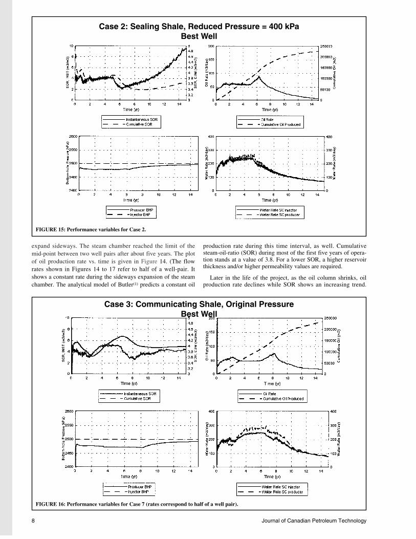
Fluid PropertiesThe bitumen viscosity vs. temperature behaviour is depicted in

Figure 11, and is essentially the one used by other researchers(4, 5)

studying McMurray bitumen. Three components were chosen,water, bitumen, and methane. Component properties wereobtained from other similar studies(5, 7). The bitumen was assumedwith no solution gas. This is based on the experience obtainedfrom the UTF simulation study, where the simulator predicteddevelopment of unrealistically high concentrations of the solutiongas in the steam chamber while the pilot data provided no evi-dence for it. The study recommended assigning no solution gas inthe simulator to obtain realistic results(3).

Saturation FunctionsWater-oil and gas oil relative permeability curves of this study

are depicted in Figures 12 and 13(7). They indicate an irreduciblewater saturation of 0.19, residual gas saturation of 0, residual oilsaturation to water of 0.15, and residual oil saturation to gas of 0.The values for gas-oil and water-oil capillary pressure wereassigned zero(5, 7).

Well Constraints and ConditionsA horizontal well pair of 700 m length was considered. The

injection well was located 4 m above the base, while the producerwas in the first grid-block in the vertical direction. During the firsttwo months of the start-up period, a constant heat flux option wasused for both the injector and the producer, with a 200 kPa pres-sure difference to encourage early communication(5, 7). A constantsteam injection pressure of 2,500 kPa was assigned. Injectionpressure at the UTF project(3) was 2,600 kPa, and that used in theSurmont simulation studies(7) was 2,500 kPa. The producing wellin the SAGD process works under steam-trap conditions to allowproduction of produced fluids while hot and mobile, and to avoidexcessive steam production. In the simulator we assigned a maxi-

mum of 1 m3/day steam production to model the steam trapprocess. As the results indicate, typical steam injection rates werein the range of 100 – 300 m3/day. The excess steam produced wastherefore less than 1% of the injected values, and has negligibleeffects on the results.

Initial ValuesSimulation runs were conducted at two different initial pres-

sures. The simulations at the original pressure considered a pres-sure of 1,900 kPa, while the depleted gas-cap runs considered 400kPa. All of the pressures reported in this work are reported at adepth of 360 m. The original reservoir temperature was 10.5˚ C.Initial water and oil saturations were assigned, based on a metre-by-metre reading from the available logs. The remainder of theinput values is provided elsewhere(10).

Simulation ResultsA numerical simulation was conducted to study the feasibility

of bitumen production by the SAGD process, and to quantify theeffect of gas-cap depletion on the process. Thus two pressures areconsidered; cases with odd numbers are at initial reservoir pres-sure, and those with even numbers are at a reduced pressure of400 kPa (representing a depleted gas cap). Cases 1 – 8 considerthe Best-Well, and Cases 9 and 10 examine the Second-Best-Well. Four different sealing characteristics for the shale at the topof the channel are assumed. Sealing Shale (Cases 1 and 2),Partially Sealing (Cases 3 and 4), Homogeneous (Cases 5 and 6),and Communicating (Cases 7 and 8 for the Best Well, and Cases 9and 10 for the Second Best Well).

The results were studied using two types of graphs.Performance plots that depict a performance variable, e.g., oilflow rate and SOR, vs. time, and cross-sectional plots showing thedevelopment of the steam chamber. The cross-sectional plots werestudied(10), but are not shown in this paper. Three performanceparameters are considered for comparison between different cases,i.e., the time to reach 60% recovery, the average bitumen produc-tion rate, and cumulative SOR at 10 years of operation. Theresults are summarized in Tables 1 and 2. Table 1 gives the sum-mary of the individual cases, while Table 2 compares the simula-tion results of this study with those from other commercial SAGDprojects.

In the following, the results of Case 1 are described in detail,and the results of the subsequent cases are given briefly.

Case 1: Sealing Shale—Initial Pressure(Best Well)

In Cases 1 and 2, the sealing shale separates the lower bitumenfrom the top thief zones. The study of cross sectional plotsshowed the development of the steam chamber. Shortly after oneyear, steam reached the sealing shale at the top, and started to


FIGURE 11: Bitumen viscosity versus temperature. FIGURE 12: Water-oil relative permeability curves.

FIGURE 13: Gas-liquid relative permeability curves.


TABLE 1: Summary of the cases—reservoir description and results.

Case # 1 2 3 4 5 6 7 8 9 10

Reservoir Description BEST WELL 2nd Best well

Shale Characteristic at top Sealing Partial Sealing Homogeneous Communicating Communicating

Pressure at 360 m, kPa 1,900 400 1,900 400 1,900 400 1,900 400 1,900 400Gross Thickness 35 35 56 56 56 56 56 58 58Gas Thickness 0 0 6 6 6 6 6 6 6Water Thickness 0 0 2 2 2 2 2 2 2OOIP, 1,000 m3 548 544 668 662 668 664 662 608 602

Results

Average Oil Rate after 10 years, 110 109 107 108 37 103 102 32 30m3/day

Cumulative SOR at 10 years 3.4 3.4 3.3 3.2 7.5 4 4.2 8.5 10

Time to reach 60% recovery, years 7.4 7.4 10.4 9.9 >20 10.8 11.2 > 20 > 20

TABLE 2: A comparison between average oil production rate and cumulative SOR between the study area andother commercial SAGD projects.

Average Rate, m3/day Reference (Based on 700-m wells) Cum SOR

Christina Lake — 1.9Suggett (2000)(6)

Generic McMurray Formation 210 2Law et al. (2000)(4)

Generic McMurray Formation 110 2.7Good et al. (1997(5)

UTF Project Phase-B 100 2.6Mukherjee et al. (1995)(3)

Study Area 100 – 110 3.2 – 4.2 Best Well

Study Area 30 – 35 8.5 – 10Second Best Well

FIGURE 14: Performance variables for Case 1 (rates correspond to half of a well pair).

Case 1: Sealing Share, Original Pressure Best Well

expand sideways. The steam chamber reached the limit of themid-point between two well pairs after about five years. The plotof oil production rate vs. time is given in Figure 14. (The flowrates shown in Figures 14 to 17 refer to half of a well-pair. Itshows a constant rate during the sideways expansion of the steamchamber. The analytical model of Butler(1) predicts a constant oil

production rate during this time interval, as well. Cumulativesteam-oil-ratio (SOR) during most of the first five years of opera-tion stands at a value of 3.8. For a lower SOR, a higher reservoirthickness and/or higher permeability values are required.

Later in the life of the project, as the oil column shrinks, oilproduction rate declines while SOR shows an increasing trend.


FIGURE 15: Performance variables for Case 2.

FIGURE 16: Performance variables for Case 7 (rates correspond to half of a well pair).

Case 2: Sealing Shale, Reduced Pressure = 400 kPa Best Well

Case 3: Communicating Shale, Original Pressure Best Well

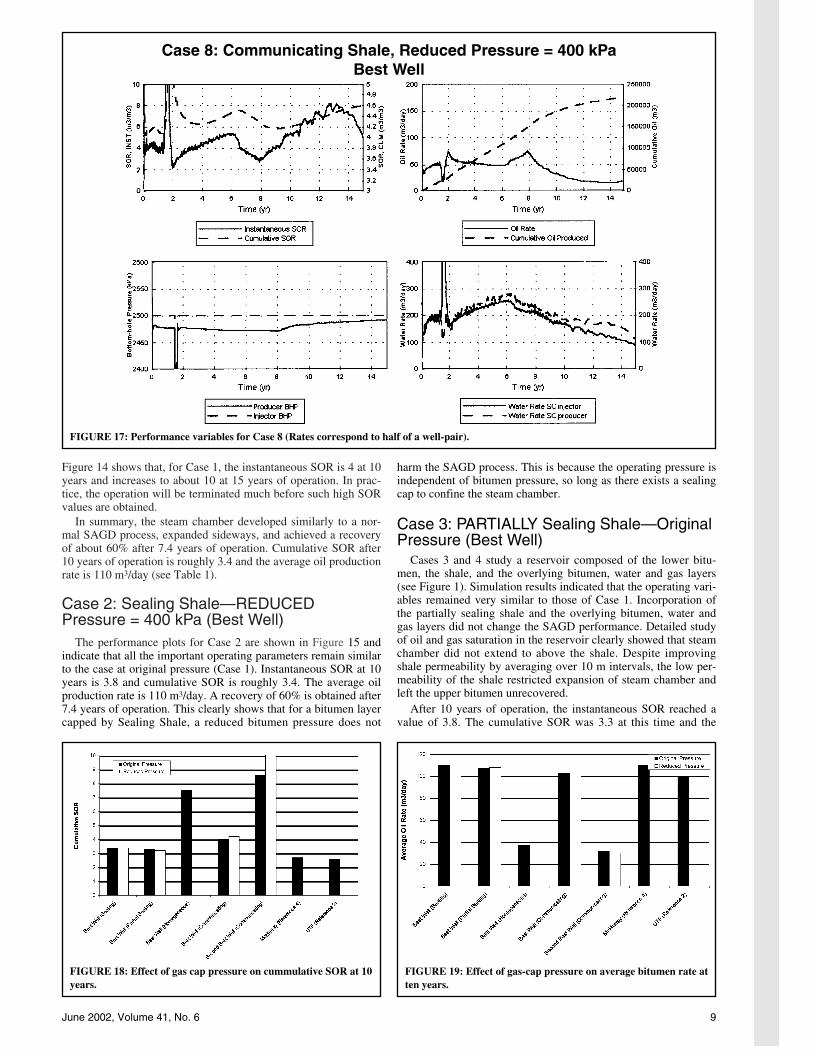
Figure 14 shows that, for Case 1, the instantaneous SOR is 4 at 10years and increases to about 10 at 15 years of operation. In prac-tice, the operation will be terminated much before such high SORvalues are obtained.

In summary, the steam chamber developed similarly to a nor-mal SAGD process, expanded sideways, and achieved a recoveryof about 60% after 7.4 years of operation. Cumulative SOR after10 years of operation is roughly 3.4 and the average oil productionrate is 110 m3/day (see Table 1).

Case 2: Sealing Shale—REDUCEDPressure = 400 kPa (Best Well)

The performance plots for Case 2 are shown in Figure 15 andindicate that all the important operating parameters remain similarto the case at original pressure (Case 1). Instantaneous SOR at 10years is 3.8 and cumulative SOR is roughly 3.4. The average oilproduction rate is 110 m3/day. A recovery of 60% is obtained after7.4 years of operation. This clearly shows that for a bitumen layercapped by Sealing Shale, a reduced bitumen pressure does not

harm the SAGD process. This is because the operating pressure isindependent of bitumen pressure, so long as there exists a sealingcap to confine the steam chamber.

Case 3: PARTIALLY Sealing Shale—OriginalPressure (Best Well)

Cases 3 and 4 study a reservoir composed of the lower bitu-men, the shale, and the overlying bitumen, water and gas layers(see Figure 1). Simulation results indicated that the operating vari-ables remained very similar to those of Case 1. Incorporation ofthe partially sealing shale and the overlying bitumen, water andgas layers did not change the SAGD performance. Detailed studyof oil and gas saturation in the reservoir clearly showed that steamchamber did not extend to above the shale. Despite improvingshale permeability by averaging over 10 m intervals, the low per-meability of the shale restricted expansion of steam chamber andleft the upper bitumen unrecovered.

After 10 years of operation, the instantaneous SOR reached avalue of 3.8. The cumulative SOR was 3.3 at this time and the


FIGURE 18: Effect of gas cap pressure on cummulative SOR at 10years.

FIGURE 17: Performance variables for Case 8 (Rates correspond to half of a well-pair).

Case 8: Communicating Shale, Reduced Pressure = 400 kPa Best Well

FIGURE 19: Effect of gas-cap pressure on average bitumen rate atten years.

average oil production rate is 107 m3/day. The main differencebetween results of Case 3 and Case 1 is that it took a longer timeto recover 60% of the bitumen (10.4 years). This was because theoriginal bitumen in place includes the bitumen of the upper sands.Little of that bitumen, however, was recovered. The summary ofthe results is shown in Figures 18, 19, and 20. Results are shownat original and reduced gas-cap pressure for all shale behavioursconsidered.

Case 4: PARTIALLY Sealing Shale—REDUCED Pressure = 400 kPa (Best Well)

In Case 4, the initial pressure was lowered to simulate prior gasproduction. The simulation results indicated very similar perfor-mance variables (See Figures 18 to 20). The results of Case 4indicated that reduced gas-cap pressure did not harm bitumenrecovery.

Case 5: Homogeneous Formation—OriginalPressure (Best well)

In Cases 5 and 6, the distribution of bitumen, water and gas isthe same as in Cases 3 and 4. Here, the shale and sand layers wereassigned an average permeability throughout. Performance plotsindicated an uneconomic performance(10). The average oil produc-tion rate was below 40 m3/day over the first 10 years. CumulativeSOR at 10 years was 7.5 (See Table 1 and Figures 18 to 20).

Case 6: Homogeneous Formation—REDUCED Pressure = 400 kPa (Best well)

The Case 5 study revealed that, with the geological model con-sidered, economic bitumen production by the SAGD process isnot feasible. Therefore, the study of the effect of pressure deple-tion was felt to be redundant.

Case 7: Communicating Shale—OriginalPressure (Best Well)

In Cases 7 and 8, the distribution of bitumen, water and gas isthe same as in Cases 3 to 5. The shale characteristics, and perme-ability distribution are also the same as in Cases 3 – 5, with theimportant exception that there are no permeability layers with val-ues less than 200 and 50 mD for the horizontal and vertical per-meability, respectively. The simulation results indicated that theimprovement in shale permeability and led to steam chamber riseinto the upper sands. As shown in Figure 16, after 10 years ofoperation, instantaneous and cumulative SOR stand at 3.8 and 4.The average oil production rate during the first 10 years is 103m3/day. It takes about 11 years to achieve a recovery of 60%.

Case 8: Communicating Shale—REDUCED

Pressure = 400 kPa (Best Well)

Operating parameters have deteriorated slightly (see Figure17). After 10 years of operations, the average oil production rateis 102 m3/day (compared with 103 m3/day at the original pres-sure), and the cumulative SOR 4.2 (compared with 4 at the origi-nal pressure). Figure 21 shows bitumen recovery as a function oftime for Cases 7 and 8. It can be seen that a lower gas-cap pres-sure results in a slight deceleration of recovery. It takes 10.8 and11.2 years for a recovery of 60%, when the gas-cap pressure is1,900 and 400 kPa, respectively.

Case 9: SECOND Best Well—Communicating Shale—Original Pressure

In order not to be biased by the performance of the best well,bitumen production from a reservoir exhibiting reservoir qualityof the second best well, depicted in Figure 2, was studied in Case9. The effect of gas production on the SAGD process was investi-gated in Case 10. It was felt that the largest effect of gas-cap pres-sure is obtained when the communicating shale approach is imple-mented. This is because the communicating shale approach allowsexpansion of the steam chamber into the upper sands.

The performance plots indicated a poor project because of poorformation quality. After 20 years of operation recovery is only40%. The cumulative and instantaneous SOR are above 8 (SeeTable 1). The average oil production rate during the first 10 yearsis only 32 m3/day.

Case 10: SECOND Best Well—Communicating Shale—Reduced Pressure =400 kPa

A study of the cross-sectional plots indicated that the high per-meability assigned to the shale layers permitted communicationwith the upper sands. Operating parameters were unattractive atthe original pressure. The results indicated that they remainedunattractive at lower gas-cap pressure, and have deterioratedsomewhat. After 10 years of operations, the average oil produc-tion rate is 30 m3/day (compared with 32 m3/day at the originalpressure), and cumulative SOR is 10 (compared with the 8.5 at theoriginal pressure).

Other Sensitivity StudiesIn addition to the cases reported above, other sensitivity studies

were conducted to examine the effect of gas-cap size and the aver-aging method used. The results of these runs have been recentlysubmitted to EUB(16). For brevity here, we will restrict ourselvesto a brief review of the results.


FIGURE 21: Effect of gas-cap pressure on recover (best well,communicating shale, Cases 7 and 8).

FIGURE 20: Effect of gas-cap pressure on time to reach 60%recovery.

Effect of Gas-Cap SizeIn Cases 1 to 10, we considered a gas-cap size of the same lat-

eral extent as the reservoir. A limited gas-cap size allowed theinjection pressure to remain above the gas-cap pressure, even aftercommunication was established between the steam chamber andthe gas cap. This configuration, which represents a well pair sur-rounded by neighbouring well pairs, was chosen because most ofthe operating wells in a SAGD project would be offset by otheroperating well-pairs. Also, the small size of the gas reserves foundfrom the geological study(10) suggests a limited extent to the gascap. Nevertheless, simulations were performed where the lateralsize of the top 8 m consisting of the gas cap and top water wasdoubled for the Best Well. The results indicated that doubling ofthe top sands had a small effect. The cumulative SOR at changedby 0.2 units and recovery was delayed by about four months.

Effect of Averaging IntervalIn Cases 3 – 4 and 7 – 10 the shale content and porosity were

averaged over a vertical window of 10 m and were then used inthe power-law averaging equation. This resulted in smearing ofthe high and low permeability values and may be consideredunphysical(17). To examine this, two more runs were conductedwhere similar to Cases 1 and 2, porosity and shale volumes on ametre-by-metre basis were directly used in the averaging equa-tion. Then, the low permeability values were removed by increas-ing the low horizontal permeability values to 200 mD and the lowvertical permeability values to 50 mD. In this way, communica-tion through the shale was allowed, while the sand permeabilitywas estimated using its own petrophysical data. The differencebetween results with 10 m averaging (Cases 7 and 8) and the tworecent runs with 1 m was very small.

DiscussionThe simulation study of this work was meant to provide

answers to two important questions, namely, what are the impor-tant performance parameters of a SAGD operation for the case ofinterest, and what are the effects of gas-cap production on the per-formance of such a thermal recovery process. To obtain theanswers, one of the most important factors affecting the answers,i.e., the connectivity of the upper shale layer, was carefully inves-tigated. A methodology was developed to investigate differentscenarios with respect to shale characteristics. There are factorsother than the shales and the gas-cap size that have an effect onthe SAGD operation. These were not studied in the sensitivityruns, and are considered to be of secondary importance. Some ofthese are reviewed in the following.

SAGD optimization methods were not included. Injection ofnon-condensable gases and blow-down of the steam chamber bystopping the injection while continuing oil production couldimprove thermal efficiency of the process. Both of these methodstend to reduce oil production rate.

• Experience from the UTF simulation study(3) indicated that afluctuation in vertical distance between the injector and pro-ducer along the wells would result in a non-uniform steamdistribution in that direction. By assigning one grid block inthe Y direction, uniform steam distribution was implied. 2Dmodelling of the process has been reported to overestimateSAGD performance. The UTF experience clearly indicatesthat non-uniform steam distribution has a major effect ondelaying the start-up period of the project(3).

• Operational problems such as lack of enough steam were notincluded.

• High injection pressures, which can lead to geomechanicalalteration of reservoir properties, were not considered.

It is also important to discuss the similarities and the differ-ences between top-water and top-gas layers directly above aSAGD steam chamber and their effect on the operation. First, con-sider a bitumen reservoir overlain by a finite gas cap. SAGD oper-

ation in such a reservoir could be initiated ignoring the effect ofthe gas cap. The high viscosity of the in situ bitumen isolates thesteam chamber from the gas cap. As the steam chamber approach-es the gas cap, and if the steam pressure is kept higher than thegas-cap pressure, steam and possibly some of the oil is pushedinto the gas cap. In a well pair surrounded by other operatingwells, which are typically about 100 m away, steam would flowinto the finite gas cap until there is little pressure differencebetween the steam chamber and the gas cap. Furthermore, thesteam would condense upon contact with the cold reservoir at top,and due to continued heat-loss through the enlarged contact areawith the overburden. This would require the flow of more steamto replace the condensed steam. One blessing is that, the presenceof non-condensable gases would lead to a reduced partial pressureof the steam in the gas cap. This, in turn, would allow the steam toremain in the gaseous phase down to much lower temperatures ascompared to steam in the steam chamber and would reduce theamount of additional steam needed. For the case of a top-waterlayer, the situation is much different. The amount of heat con-sumed in the upper sand is much more than that in a gas cap,because of the much higher heat capacity of water and no partial-pressure advantage. Furthermore, water might drain into the steamchamber leading to either a collapsed steam chamber or requiringmuch higher injection rates. Some simulation studies have indicat-ed that water might be kept at the top of the steam chamber(5),while others have not observed this effect(4). It can be imaginedthat, for thick water sands, a free surface would develop betweenthe steam and the water, much similar to the air-water free surfacethat develops in earth dams(18). Interactions at the steam-water freesurface are much more complicated than that observed in an earthdam, due to the condensation of steam and possible movement ofthis free surface. Nevertheless, an important similarity is that thewater would drain along the free surface, and further downstreaminto the steam chamber, reducing the thermal efficiency of theprocess.

Summary and ConclusionsA simulation study was conducted to examine the feasibility of

bitumen production from a project area in Alberta using theSAGD process, and to determine the effect of gas-cap productionon the process. Bitumen recovery, average oil production rate andcumulative steam-oil ratio (SOR) are the three main parametersused for evaluation of the attractiveness of bitumen recovery oper-ations. Studies were conducted using petrophysical properties ofthe Best and Second Best Well. These performance parameterswere compared with some of the corresponding values reportedand/or forecast for economically feasible operations, such as theUTF and Christina Lake projects (see Table 2 and Figures 18 and19). The effect of pressure reduction (due to gas-cap production)on bitumen recovery, rate, and SOR was investigated.

Four representations of the shale layers were examined. Thefollowing summarizes the conclusions of this study.

1. Average oil production rate for the Best and Second Bestwells in the lands were 100 – 110 m3/day and 30 – 35m3/day, respectively. Corresponding cumulative SOR valuesare 3.2 – 4.2 and 8 – 10, respectively.

2. The results of the simulation studies at the original pressureand after gas-cap depletion indicate that, for the cases inves-tigated, gas production leading to lower initial pressure has asmall effect on the SAGD performance parameters. Forexample for the Best Well with communicating shale, gascap depletion to 400 kPa resulted in approximately fivemonths delay to reach the same 60% recovery and 0.2-unitsincrease at ten years. Gas cap pressure had no effect whensteam chamber did not expand through the top shale.

3. It was shown that operating pressure, is independent of ini-tial pressure so long as there is a cap confining the verticalexpansion of the steam chamber.

REFERENCES


1. BUTLER, R.M., Thermal Recovery of Oil and Bitumen; Calgary,AB, 1997.

2. EDMUNDS, N.R., KOVALSKY, S.D., GITTINS, S.D., and PEN-NACCHIOLI, E.D., Review of Phase A Steam-Assisted GravityDrainge Test; SPE Reservoir Engineering, pp. 119-124, May 1994.

3. MUKHERJEE, N.J., GITTINS, S.D., EDMUNDS, N.R., andKISMAN, K.E., A Comparison of Field Vs. Forecast Performancefor Phase B of the UTF SAGD Project in the Athabasca Oil Sands;paper presented at the 6th UNITAR International Conference onHeavy Crude and Tar Sands, Houston,TX, February 1995.

4. LAW, D.H.S., RAWFIK, N.N., GOOD, W.K., Field-ScaleNumerical Simulation of SAGD Process with Top-Water ThiefZone; paper SPE 65522 presented at the 2000 SPE/the PetroleumSociety International Conference on Horizontal Well Technology,Calgary, AB, November 6 – 8, 2000.

5. GOOD, W.K., CLAUDE, R., and FETLY, B.D., Possible Effects ofGas Caps on SAGD Performance; ADOE/EUB Report, 1997.

6. SUGGETT, J., GITTINS, S.D., and YOUNG, S., Christina LakeThermal Project; paper SPE 65520 presented at the 2000SPE/Petroleum Society International Conference on Horizontal WellTechnology, Calgary, AB, November 6 – 8, 2000.

7. Documents accompanying Gas-Bitumen Enquiry and SurmontHearing; available at Alberta EUB 1997 – 1999.

8. ITO, Y., SUZUKI, S., and YAMADA, H., Effect of ReservoirParameters on Oil Rate and Steam-Oil Ratio in SAGD Project; paperpresented at the 7th UNITAR International Conference on HeavyCrude and Tar Sands, Beijing, China, October 27 – 31, 1998.

9. EDMUNDS, N. and CHHINA, H., Economic Optimum OperatingPressure for SAGD Projects in Alberta; Journal of CanadianPetroleum Technology Vol. 40 (12), pp. 13-17, December 2001.

10. Anderson’s submission to EUB, January 2001; Part of Devon’s evi-dence in Alberta EUB Chard/Leismer Gas-Bitumen Hearing,November 2001 – May 2002.

11. DEUTSCH, V.C.: Geostatistical Reservoir Modelling; OxfordUniversity Press, 2001.

12. DEUTSCH, V.C., Calculating Effective Absolute Permeability inSandstone/Shale Sequences; SPE Formation Evaluation, pp. 343-348, September 1989.

13. MAGARA, K., Porosity-Permeability Relationship of Shales; unso-licited SPE paper 2430.

14. BORST, R., Methods for Calculating Shale Permeability; unsolicitedSPE paper 11768.

15. SOEDER, D.J., Porosity and Permeability of Eastern Devonian GasShale; paper SPE 15213 presented at the 1986 Unconventional GasSymposium, Louisville, KY, May 18 – 21.

16. Devon’s undertakings; Part of Alberta EUB Chard/Leismer Gas-Bitumen Hearing, November 2001 – May 2002.

17. DEAUTSCH, C.V. ; personal communication, April 2002.18. BEAR, J., Dynamics of Fluids in Porous Media; Dove Publication,

N.Y., 1972.

AcknowledgmentsThe authors gratefully acknowledge numerous discussions with

Ms. Lisa Dean on the geology and Mr. Colin Jordan on the reser-voir engineering.


Authors’ Biographies

Mehran Pooladi-Darvish is an associateprofessor of petroleum engineering at theUniversity of Calgary where he teachesReservoir Engineering and Well Testingcourses. His current research activities areon experimental and modelling studies ofcold production of heavy oil, upscalingmethods in naturally fractured reservoirs,and gas production from hydrate reservoirs.Mehran’s work experience includes con-sulting in Calgary, research at Reservoir

Engineering Research Institute in Palo Alto, California, and reser-voir engineering practice in Ahwaz, Iran. Mehran received a B.Sc.in chemical engineering (1989) and an M.Sc. in chemical andpetroleum engineering (1992) from Iran. He graduated with aPh.D. in petroleum engineering from the University of Alberta(1995). He is a member of APEGGA, the Petroleum Society, SPE,and CSChE.

Louis Mattar is the president of FeketeAssociates Inc. He has co-authored over 35publications including the ERCB guide G-3Gas Well Testing—Theory and Practice.He is a member of APPEGA, SPE, and thePetroleum Society. He graduated from theUniversity of Calgary with an M.Sc. degreein 1973.

REFERENCES

June 2002, Volume 41, No. 6 11